Analysing ventilation efficiency in a test chamber using age-of-air concept and CFD technology
13
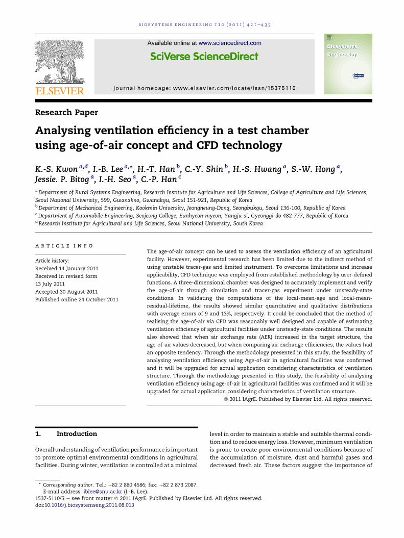
Research Paper Analysing ventilation efficiency in a test chamber using age-of-air concept and CFD technology K.-S. Kwon a,d , I.-B. Lee a, *, H.-T. Han b , C.-Y. Shin b , H.-S. Hwang a , S.-W. Hong a , Jessie. P. Bitog a , I.-H. Seo a , C.-P. Han c a Department of Rural Systems Engineering, Research Institute for Agriculture and Life Sciences, College of Agriculture and Life Sciences, Seoul National University, 599, Gwanakno, Gwanakgu, Seoul 151-921, Republic of Korea b Department of Mechanical Engineering, Kookmin University, Jeongneung-Dong, Seongbukgu, Seoul 136-100, Republic of Korea c Department of Automobile Engineering, Seojeong College, Eunhyeon-myeon, Yangju-si, Gyeonggi-do 482-777, Republic of Korea d Research Institute for Agricultural and Life Sciences, Seoul National University, South Korea article info Article history: Received 14 January 2011 Received in revised form 13 July 2011 Accepted 30 August 2011 Published online 24 October 2011 The age-of-air concept can be used to assess the ventilation efficiency of an agricultural facility. However, experimental research has been limited due to the indirect method of using unstable tracer-gas and limited instrument. To overcome limitations and increase applicability, CFD technique was employed from established methodology by user-defined functions. A three-dimensional chamber was designed to accurately implement and verify the age-of-air through simulation and tracer-gas experiment under unsteady-state conditions. In validating the computations of the local-mean-age and local-mean- residual-lifetime, the results showed similar quantitative and qualitative distributions with average errors of 9 and 13%, respectively. It could be concluded that the method of realising the age-of-air via CFD was reasonably well designed and capable of estimating ventilation efficiency of agricultural facilities under unsteady-state conditions. The results also showed that when air exchange rate (AER) increased in the target structure, the age-of-air values decreased, but when comparing air exchange efficiencies, the values had an opposite tendency. Through the methodology presented in this study, the feasibility of analysing ventilation efficiency using Age-of-air in agricultural facilities was confirmed and it will be upgraded for actual application considering characteristics of ventilation structure. Through the methodology presented in this study, the feasibility of analysing ventilation efficiency using age-of-air in agricultural facilities was confirmed and it will be upgraded for actual application considering characteristics of ventilation structure. ª 2011 IAgrE. Published by Elsevier Ltd. All rights reserved. 1. Introduction Overall understanding of ventilation performance is important to promote optimal environmental conditions in agricultural facilities. During winter, ventilation is controlled at a minimal level in order to maintain a stable and suitable thermal condi- tion and to reduce energy loss. However, minimum ventilation is prone to create poor environmental conditions because of the accumulation of moisture, dust and harmful gases and decreased fresh air. These factors suggest the importance of * Corresponding author. Tel.: þ82 2 880 4586; fax: þ82 2 873 2087. E-mail address: [email protected] (I.-B. Lee). Available online at www.sciencedirect.com journal homepage: www.elsevier.com/locate/issn/15375110 biosystems engineering 110 (2011) 421 e433 1537-5110/$ e see front matter ª 2011 IAgrE. Published by Elsevier Ltd. All rights reserved. doi:10.1016/j.biosystemseng.2011.08.013
Transcript of Analysing ventilation efficiency in a test chamber using age-of-air concept and CFD technology
ww.sciencedirect.com
b i o s y s t em s e ng i n e e r i n g 1 1 0 ( 2 0 1 1 ) 4 2 1e4 3 3
Available online at w
journal homepage: www.elsev ier .com/locate/ issn/15375110
Research Paper
Analysing ventilation efficiency in a test chamberusing age-of-air concept and CFD technology
K.-S. Kwon a,d, I.-B. Lee a,*, H.-T. Han b, C.-Y. Shin b, H.-S. Hwang a, S.-W. Hong a,Jessie. P. Bitog a, I.-H. Seo a, C.-P. Han c
aDepartment of Rural Systems Engineering, Research Institute for Agriculture and Life Sciences, College of Agriculture and Life Sciences,
Seoul National University, 599, Gwanakno, Gwanakgu, Seoul 151-921, Republic of KoreabDepartment of Mechanical Engineering, Kookmin University, Jeongneung-Dong, Seongbukgu, Seoul 136-100, Republic of KoreacDepartment of Automobile Engineering, Seojeong College, Eunhyeon-myeon, Yangju-si, Gyeonggi-do 482-777, Republic of KoreadResearch Institute for Agricultural and Life Sciences, Seoul National University, South Korea
a r t i c l e i n f o
Article history:
Received 14 January 2011
Received in revised form
13 July 2011
Accepted 30 August 2011
Published online 24 October 2011
* Corresponding author. Tel.: þ82 2 880 4586E-mail address: [email protected] (I.-B. Lee
1537-5110/$ e see front matter ª 2011 IAgrEdoi:10.1016/j.biosystemseng.2011.08.013
The age-of-air concept can be used to assess the ventilation efficiency of an agricultural
facility. However, experimental research has been limited due to the indirect method of
using unstable tracer-gas and limited instrument. To overcome limitations and increase
applicability, CFD technique was employed from established methodology by user-defined
functions. A three-dimensional chamber was designed to accurately implement and verify
the age-of-air through simulation and tracer-gas experiment under unsteady-state
conditions. In validating the computations of the local-mean-age and local-mean-
residual-lifetime, the results showed similar quantitative and qualitative distributions
with average errors of 9 and 13%, respectively. It could be concluded that the method of
realising the age-of-air via CFD was reasonably well designed and capable of estimating
ventilation efficiency of agricultural facilities under unsteady-state conditions. The results
also showed that when air exchange rate (AER) increased in the target structure, the
age-of-air values decreased, but when comparing air exchange efficiencies, the values had
an opposite tendency. Through the methodology presented in this study, the feasibility of
analysing ventilation efficiency using Age-of-air in agricultural facilities was confirmed
and it will be upgraded for actual application considering characteristics of ventilation
structure. Through the methodology presented in this study, the feasibility of analysing
ventilation efficiency using age-of-air in agricultural facilities was confirmed and it will be
upgraded for actual application considering characteristics of ventilation structure.
ª 2011 IAgrE. Published by Elsevier Ltd. All rights reserved.
1. Introduction level in order to maintain a stable and suitable thermal condi-
Overall understanding of ventilationperformance is important
to promote optimal environmental conditions in agricultural
facilities. During winter, ventilation is controlled at a minimal
; fax: þ82 2 873 2087.).. Published by Elsevier Lt
tion and to reduce energy loss. However,minimumventilation
is prone to create poor environmental conditions because of
the accumulation of moisture, dust and harmful gases and
decreased fresh air. These factors suggest the importance of
d. All rights reserved.
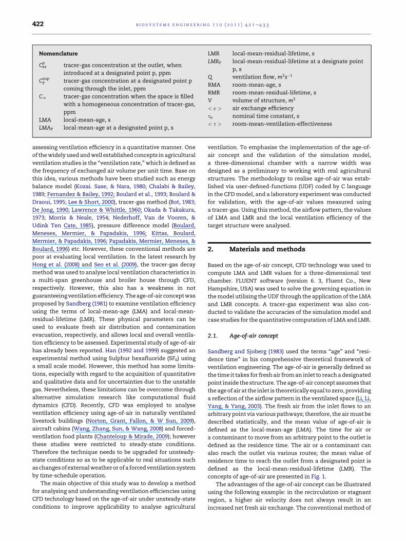
Nomenclature
Cpex tracer-gas concentration at the outlet, when
introduced at a designated point p, ppm
CsupP tracer-gas concentration at a designated point p
coming through the inlet, ppm
CN tracer-gas concentration when the space is filled
with a homogeneous concentration of tracer-gas,
ppm
LMA local-mean-age, s
LMAP local-mean-age at a designated point p, s
LMR local-mean-residual-lifetime, s
LMRP local-mean-residual-lifetime at a designate point
p, s
Q ventilation flow, m3s�1
RMA room-mean-age, s
RMR room-mean-residual-lifetime, s
V volume of structure, m3
< ε > air exchange efficiency
sn nominal time constant, s
< s > room-mean-ventilation-effectiveness
b i o s y s t em s e n g i n e e r i n g 1 1 0 ( 2 0 1 1 ) 4 2 1e4 3 3422
assessing ventilation efficiency in a quantitative manner. One
of thewidelyusedandwell established concepts in agricultural
ventilation studies is the “ventilation rate,” which is defined as
the frequency of exchanged air volume per unit time. Base on
this idea, various methods have been studied such as energy
balance model (Kozai. Sase, & Nara, 1980; Chalabi & Bailey,
1989; Fernandez & Bailey, 1992; Boulard et al., 1993; Boulard &
Draoui, 1995; Lee & Short, 2000), tracer-gas method (Bot, 1983;
De Jong, 1990; Lawrence & Whittle, 1960; Okada & Takakura,
1973; Morris & Neale, 1954; Nederhoff, Van de Vooren, &
Udink Ten Cate, 1985), pressure difference model (Boulard,
Meneses, Mermier, & Papadakis, 1996; Kittas, Boulard,
Mermier, & Papadakis, 1996; Papadakis, Mermier, Meneses, &
Boulard, 1996) etc. However, these conventional methods are
poor at evaluating local ventilation. In the latest research by
Hong et al. (2008) and Seo et al. (2009), the tracer-gas decay
methodwas used to analyse local ventilation characteristics in
a multi-span greenhouse and broiler house through CFD,
respectively. However, this also has a weakness in not
guaranteeingventilationefficiency.Theage-of-air conceptwas
proposed by Sandberg (1981) to examine ventilation efficiency
using the terms of local-mean-age (LMA) and local-mean-
residual-lifetime (LMR). These physical parameters can be
used to evaluate fresh air distribution and contamination
evacuation, respectively, and allows local and overall ventila-
tion efficiency to be assessed. Experimental study of age-of-air
has already been reported. Han (1992 and 1999) suggested an
experimental method using Sulphur hexafluoride (SF6) using
a small scale model. However, this method has some limita-
tions, especially with regard to the acquisition of quantitative
and qualitative data and for uncertainties due to the unstable
gas. Nevertheless, these limitations can be overcome through
alternative simulation research like computational fluid
dynamics (CFD). Recently, CFD was employed to analyse
ventilation efficiency using age-of-air in naturally ventilated
livestock buildings (Norton, Grant, Fallon, & W Sun, 2009),
aircraft cabins (Wang, Zhang, Sun, & Wang, 2008) and forced-
ventilation food plants (Chanteloup & Mirade, 2009); however
these studies were restricted to steady-state conditions.
Therefore the technique needs to be upgraded for unsteady-
state conditions so as to be applicable to real situations such
aschangesofexternalweatherorofa forcedventilationsystem
by time-schedule operation.
The main objective of this study was to develop a method
for analysing and understanding ventilation efficiencies using
CFD technology based on the age-of-air under unsteady-state
conditions to improve applicability to analyse agricultural
ventilation. To emphasise the implementation of the age-of-
air concept and the validation of the simulation model,
a three-dimensional chamber with a narrow width was
designed as a preliminary to working with real agricultural
structures. The methodology to realise age-of-air was estab-
lished via user-defined-functions (UDF) coded by C language
in the CFDmodel, and a laboratory experiment was conducted
for validation, with the age-of-air values measured using
a tracer-gas. Using thismethod, the airflowpattern, the values
of LMA and LMR and the local ventilation efficiency of the
target structure were analysed.
2. Materials and methods
Based on the age-of-air concept, CFD technology was used to
compute LMA and LMR values for a three-dimensional test
chamber. FLUENT software (version 6. 3, Fluent Co., New
Hampshire, USA) was used to solve the governing equation in
themodel utilising theUDF through the application of the LMA
and LMR concepts. A tracer-gas experiment was also con-
ducted to validate the accuracies of the simulation model and
case studies for thequantitative computation of LMAand LMR.
2.1. Age-of-air concept
Sandberg and Sjoberg (1983) used the terms “age” and “resi-
dence time” in his comprehensive theoretical framework of
ventilation engineering. The age-of-air is generally defined as
the time it takes for freshair froman inlet to reachadesignated
point inside the structure. Theage-of-air concept assumes that
theageof air at the inlet is theoretically equal to zero, providing
a reflection of the airflow pattern in the ventilated space (Li, Li,
Yang, & Yang, 2003). The fresh air from the inlet flows to an
arbitrary point via various pathways; therefore, the airmust be
described statistically, and the mean value of age-of-air is
defined as the local-mean-age (LMA). The time for air or
a contaminant to move from an arbitrary point to the outlet is
defined as the residence time. The air or a contaminant can
also reach the outlet via various routes; the mean value of
residence time to reach the outlet from a designated point is
defined as the local-mean-residual-lifetime (LMR). The
concepts of age-of-air are presented in Fig. 1.
The advantages of the age-of-air concept can be illustrated
using the following example: in the recirculation or stagnant
region, a higher air velocity does not always result in an
increased net fresh air exchange. The conventional method of
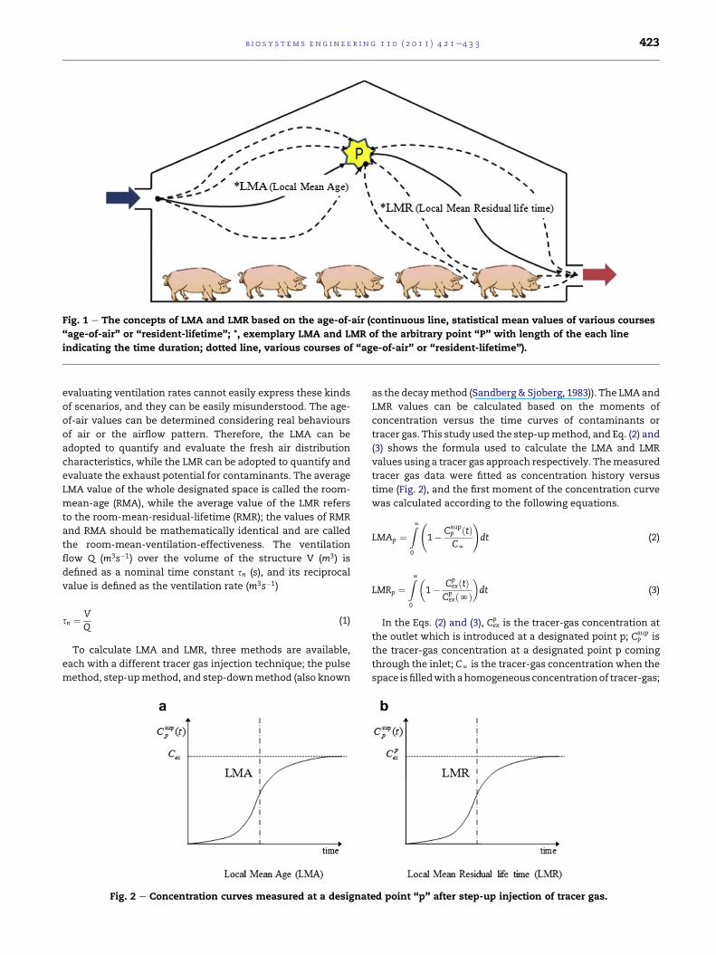
Fig. 1 e The concepts of LMA and LMR based on the age-of-air (continuous line, statistical mean values of various courses
“age-of-air” or “resident-lifetime”; *, exemplary LMA and LMR of the arbitrary point “P” with length of the each line
indicating the time duration; dotted line, various courses of “age-of-air” or “resident-lifetime”).
b i o s y s t em s e ng i n e e r i n g 1 1 0 ( 2 0 1 1 ) 4 2 1e4 3 3 423
evaluating ventilation rates cannot easily express these kinds
of scenarios, and they can be easily misunderstood. The age-
of-air values can be determined considering real behaviours
of air or the airflow pattern. Therefore, the LMA can be
adopted to quantify and evaluate the fresh air distribution
characteristics, while the LMR can be adopted to quantify and
evaluate the exhaust potential for contaminants. The average
LMA value of the whole designated space is called the room-
mean-age (RMA), while the average value of the LMR refers
to the room-mean-residual-lifetime (RMR); the values of RMR
and RMA should be mathematically identical and are called
the room-mean-ventilation-effectiveness. The ventilation
flow Q (m3s�1) over the volume of the structure V (m3) is
defined as a nominal time constant sn (s), and its reciprocal
value is defined as the ventilation rate (m3s�1)
sn ¼ VQ
(1)
To calculate LMA and LMR, three methods are available,
each with a different tracer gas injection technique; the pulse
method, step-upmethod, and step-downmethod (also known
Fig. 2 e Concentration curves measured at a designat
as the decaymethod (Sandberg& Sjoberg, 1983)). The LMA and
LMR values can be calculated based on the moments of
concentration versus the time curves of contaminants or
tracer gas. This study used the step-upmethod, and Eq. (2) and
(3) shows the formula used to calculate the LMA and LMR
values using a tracer gas approach respectively. Themeasured
tracer gas data were fitted as concentration history versus
time (Fig. 2), and the first moment of the concentration curve
was calculated according to the following equations.
LMAp ¼ZN0
1� Csup
p ðtÞCN
!dt (2)
LMRp ¼ZN0
�1� Cp
exðtÞCpexðNÞ
�dt (3)
In the Eqs. (2) and (3), Cpex is the tracer-gas concentration at
the outlet which is introduced at a designated point p; CsupP is
the tracer-gas concentration at a designated point p coming
through the inlet; CN is the tracer-gas concentration when the
space isfilledwithahomogeneous concentrationof tracer-gas;
ed point “p” after step-up injection of tracer gas.
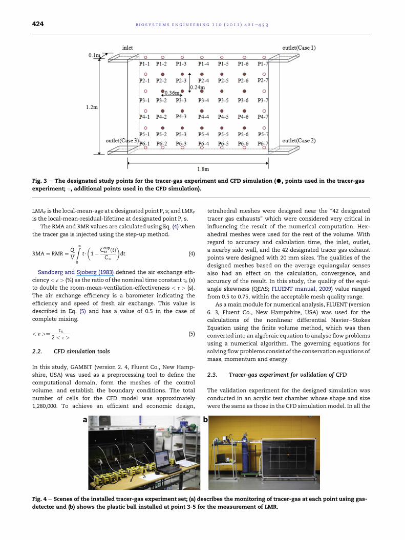
Fig. 3 e The designated study points for the tracer-gas experiment and CFD simulation (C, points used in the tracer-gas
experiment; B, additional points used in the CFD simulation).
b i o s y s t em s e n g i n e e r i n g 1 1 0 ( 2 0 1 1 ) 4 2 1e4 3 3424
LMAP is the local-mean-age at a designatedpoint P, s; and LMRP
is the local-mean-residual-lifetime at designated point P, s.
The RMA and RMR values are calculated using Eq. (4) when
the tracer gas is injected using the step-up method.
RMA ¼ RMR ¼ QV
ZN0
t$
�1� Csup
ex ðtÞCN
�dt (4)
Sandberg and Sjoberg (1983) defined the air exchange effi-
ciency< ε > (%) as the ratio of the nominal time constant sn (s)
to double the room-mean-ventilation-effectiveness < s > (s).
The air exchange efficiency is a barometer indicating the
efficiency and speed of fresh air exchange. This value is
described in Eq. (5) and has a value of 0.5 in the case of
complete mixing.
< ε >¼ sn2 < s >
(5)
2.2. CFD simulation tools
In this study, GAMBIT (version 2. 4, Fluent Co., New Hamp-
shire, USA) was used as a preprocessing tool to define the
computational domain, form the meshes of the control
volume, and establish the boundary conditions. The total
number of cells for the CFD model was approximately
1,280,000. To achieve an efficient and economic design,
Fig. 4 e Scenes of the installed tracer-gas experiment set; (a) des
detector and (b) shows the plastic ball installed at point 3-5 for
tetrahedral meshes were designed near the “42 designated
tracer gas exhausts” which were considered very critical in
influencing the result of the numerical computation. Hex-
ahedral meshes were used for the rest of the volume. With
regard to accuracy and calculation time, the inlet, outlet,
a nearby side wall, and the 42 designated tracer gas exhaust
points were designed with 20 mm sizes. The qualities of the
designed meshes based on the average equiangular senses
also had an effect on the calculation, convergence, and
accuracy of the result. In this study, the quality of the equi-
angle skewness (QEAS; FLUENT manual, 2009) value ranged
from 0.5 to 0.75, within the acceptable mesh quality range.
As a main module for numerical analysis, FLUENT (version
6. 3, Fluent Co., New Hampshire, USA) was used for the
calculations of the nonlinear differential NaviereStokes
Equation using the finite volume method, which was then
converted into an algebraic equation to analyse flow problems
using a numerical algorithm. The governing equations for
solving flowproblems consist of the conservation equations of
mass, momentum and energy.
2.3. Tracer-gas experiment for validation of CFD
The validation experiment for the designed simulation was
conducted in an acrylic test chamber whose shape and size
were the same as those in the CFD simulationmodel. In all the
cribes the monitoring of tracer-gas at each point using gas-
the measurement of LMR.
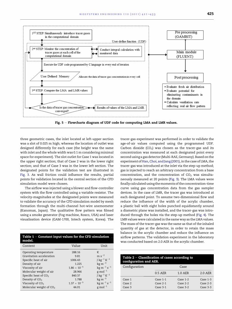
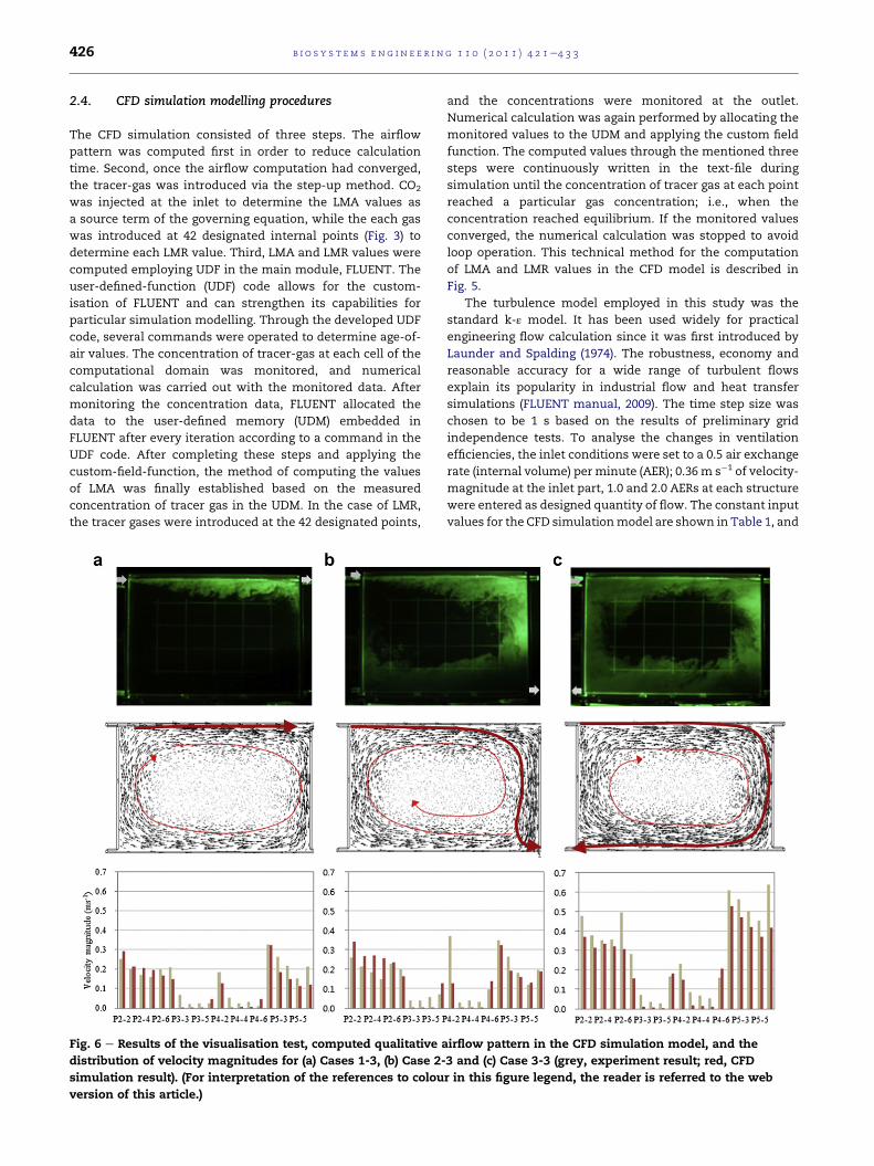
Fig. 5 e Flowcharts diagram of UDF code for computing LMA and LMR values.
b i o s y s t em s e ng i n e e r i n g 1 1 0 ( 2 0 1 1 ) 4 2 1e4 3 3 425
three geometric cases, the inlet located at left-upper section
was a slot of 0.025 m high; whereas the location of outlet was
designed differently for each case (the height was the same
with inlet and thewholewidthwas 0.1m consideringminimal
space for experiment). The slot outlet for Case 1 was located in
the upper right section; that of Case 2 was in the lower right
section; and that of Case 3 was in the lower left section. The
designated points for the validation test are illustrated in
Fig. 3. As wall friction could influence the results, partial
points for validation located in the central section of the CFD
simulation model were chosen.
The airflowwas injected using a blower and flow-controller
system with the flow controlled using a variable resistor. The
velocity-magnitudes at the designated points were measured
to validate the accuracy of the CFD simulation model by mesh
formation through the multi-channel hot-wire anemometer
(Kanomax, Japan). The qualitative flow pattern was filmed
using a smoke generator (Fog machine, Rosco, USA) and laser
visualisation device (GAM-1700, Intech system, Korea). The
Table 1 e Constant input values for the CFD simulationmodel.
Content Value Unit
Operating temperature 288.16 K
Gravitation acceleration 9.81 m s�2
Specific heat of air 1006.43 J kg�1 K�1
Density of air 1.225 kg m�3
Viscosity of air 1.86 � 10�5 kg m�1 s�1
Molecular weight of air 28.966 g mol�1
Specific heat of CO2 840.37 J kg�1 K�1
Density of CO2 1.788 kg m�3
Viscosity of CO2 1.37 � 10�5 kg m�1 s�1
Molecular weight of CO2 44.01 g mol�1
tracer-gas experiment was performed in order to validate the
age-of-air values computed using the programmed UDF.
Carbon dioxide (CO2) was chosen as the tracer-gas and its
concentration was measured at each designated point every
secondusingagasdetector (Multi-RAE,Germany). Basedonthe
experimentofHan,Choi, and Jang (2001), in thecaseofLMA,the
tracer-gas was introduced at the inlet via the step-up method;
gas is injected to reach an arbitrary concentration from a base
concentration, and the concentration of CO2 was simulta-
neously measured at 20 points (Fig. 3). The LMA values were
finallycalculatedusing themomentsof theconcentration-time
curve using gas concentration data from the gas sampler
devices. In the case of LMR, the tracer gas was introduced at
each designated point. To assume two-dimensional flow and
reduce the influence of the width of the acrylic chamber,
a plastic ball with eight holes punched equidistantly around
a diametric plane was installed, and the tracer-gas was intro-
duced through the holes via the step-up method (Fig. 4). The
LMRvalueswere calculated in the samewayas the LMAvalues.
Themass of the tracer-gas was the same as that of the inhaled
quantity of gas at the detector, in order to retain the mass
balance in the acrylic chamber and reduce the influence on
airflow patterns. The validation experiment in the laboratory
was conducted based on 2.0 AER in the acrylic chamber.
Table 2 e Classification of cases according toconfiguration and AER.
Configuration Case
0.5 AER 1.0 AER 2.0 AER
Case 1 Case 1-1 Case 1-2 Case 1-3
Case 2 Case 2-1 Case 2-2 Case 2-3
Case 3 Case 3-1 Case 3-2 Case 3-3
b i o s y s t em s e n g i n e e r i n g 1 1 0 ( 2 0 1 1 ) 4 2 1e4 3 3426
2.4. CFD simulation modelling procedures
The CFD simulation consisted of three steps. The airflow
pattern was computed first in order to reduce calculation
time. Second, once the airflow computation had converged,
the tracer-gas was introduced via the step-up method. CO2
was injected at the inlet to determine the LMA values as
a source term of the governing equation, while the each gas
was introduced at 42 designated internal points (Fig. 3) to
determine each LMR value. Third, LMA and LMR values were
computed employing UDF in the main module, FLUENT. The
user-defined-function (UDF) code allows for the custom-
isation of FLUENT and can strengthen its capabilities for
particular simulation modelling. Through the developed UDF
code, several commands were operated to determine age-of-
air values. The concentration of tracer-gas at each cell of the
computational domain was monitored, and numerical
calculation was carried out with the monitored data. After
monitoring the concentration data, FLUENT allocated the
data to the user-defined memory (UDM) embedded in
FLUENT after every iteration according to a command in the
UDF code. After completing these steps and applying the
custom-field-function, the method of computing the values
of LMA was finally established based on the measured
concentration of tracer gas in the UDM. In the case of LMR,
the tracer gases were introduced at the 42 designated points,
Fig. 6 e Results of the visualisation test, computed qualitative a
distribution of velocity magnitudes for (a) Cases 1-3, (b) Case 2-
simulation result). (For interpretation of the references to colou
version of this article.)
and the concentrations were monitored at the outlet.
Numerical calculation was again performed by allocating the
monitored values to the UDM and applying the custom field
function. The computed values through the mentioned three
steps were continuously written in the text-file during
simulation until the concentration of tracer gas at each point
reached a particular gas concentration; i.e., when the
concentration reached equilibrium. If the monitored values
converged, the numerical calculation was stopped to avoid
loop operation. This technical method for the computation
of LMA and LMR values in the CFD model is described in
Fig. 5.
The turbulence model employed in this study was the
standard k-ε model. It has been used widely for practical
engineering flow calculation since it was first introduced by
Launder and Spalding (1974). The robustness, economy and
reasonable accuracy for a wide range of turbulent flows
explain its popularity in industrial flow and heat transfer
simulations (FLUENT manual, 2009). The time step size was
chosen to be 1 s based on the results of preliminary grid
independence tests. To analyse the changes in ventilation
efficiencies, the inlet conditions were set to a 0.5 air exchange
rate (internal volume) per minute (AER); 0.36m s�1 of velocity-
magnitude at the inlet part, 1.0 and 2.0 AERs at each structure
were entered as designed quantity of flow. The constant input
values for the CFD simulationmodel are shown in Table 1, and
irflow pattern in the CFD simulation model, and the
3 and (c) Case 3-3 (grey, experiment result; red, CFD
r in this figure legend, the reader is referred to the web
b i o s y s t em s e ng i n e e r i n g 1 1 0 ( 2 0 1 1 ) 4 2 1e4 3 3 427
the classification of each case based on the configuration and
AER value is shown in Table 2.
3. Results and discussion
3.1. Validation of the accuracy of the mesh structure inthe CFD simulation model
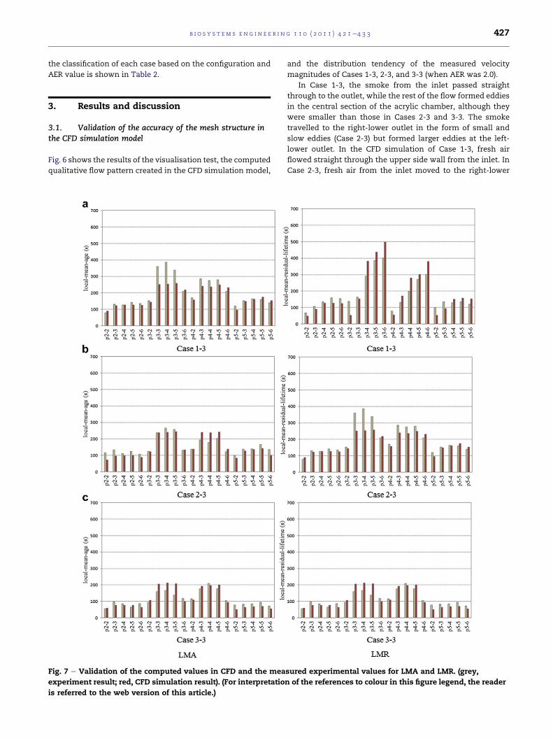
Fig. 6 shows the results of the visualisation test, the computed
qualitative flow pattern created in the CFD simulation model,
Fig. 7 e Validation of the computed values in CFD and the mea
experiment result; red, CFD simulation result). (For interpretatio
is referred to the web version of this article.)
and the distribution tendency of the measured velocity
magnitudes of Cases 1-3, 2-3, and 3-3 (when AER was 2.0).
In Case 1-3, the smoke from the inlet passed straight
through to the outlet, while the rest of the flow formed eddies
in the central section of the acrylic chamber, although they
were smaller than those in Cases 2-3 and 3-3. The smoke
travelled to the right-lower outlet in the form of small and
slow eddies (Case 2-3) but formed larger eddies at the left-
lower outlet. In the CFD simulation of Case 1-3, fresh air
flowed straight through the upper side wall from the inlet. In
Case 2-3, fresh air from the inlet moved to the right-lower
sured experimental values for LMA and LMR. (grey,
n of the references to colour in this figure legend, the reader
b i o s y s t em s e n g i n e e r i n g 1 1 0 ( 2 0 1 1 ) 4 2 1e4 3 3428
exhaust in the form of small and slow eddies. In Case 3-3,
a relatively large eddy was generated in the internal structure
compared to those in the Case 2 series, with fresh air flowing
through the sidewalls towards the left-lower exhaust.
A relatively slow air stream influenced by the large eddy in the
centre of the internal structure was also observed. These
visualisation results from the test chamber showed that the
flow pattern of each case was similar to the flow pattern of the
simulation model. Therefore, it was concluded that the CFD
simulationmodel can efficiently describe the flow pattern and
tendency in a qualitative manner.
The experiment to measure velocity-magnitude was con-
ducted for 10 min and the values were calculated on the basis
of mean velocity. The average differences in velocity-
magnitude at each point between CFD and experiment, were
0.03m s�1 (Case 1-3), 0.06m s�1 (Case 2-3), and 0.07m s�1 (Case
3-3). Comparing the correlation coefficient, Case 1-3 was 0.92,
Case 2-3 was 0.85, and Case 3-3 was 0.96, showing that the
experimental and CFD simulation results were similar, indi-
cating that the accuracy of CFD simulation for the designed
mesh structure (size 20 mm) was appropriate. This suggests
that the simulation could accurately describe theflowpatterns
and physical characteristics in a quantitative manner.
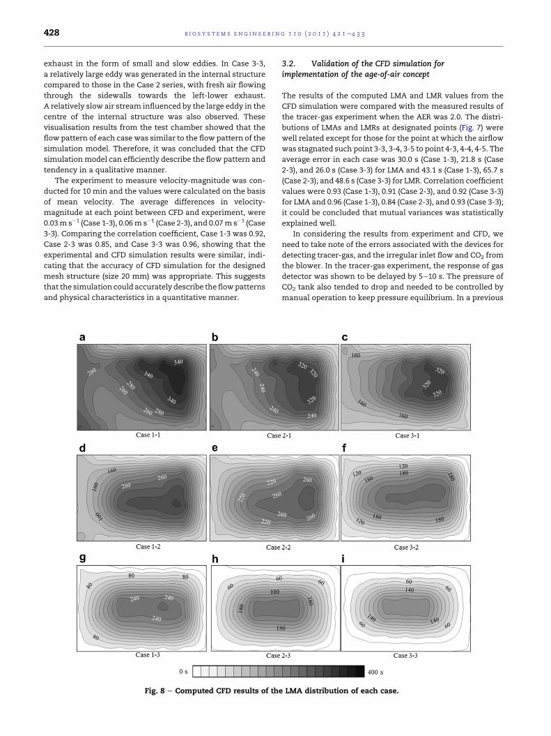
Fig. 8 e Computed CFD results of the
3.2. Validation of the CFD simulation forimplementation of the age-of-air concept
The results of the computed LMA and LMR values from the
CFD simulation were compared with the measured results of
the tracer-gas experiment when the AER was 2.0. The distri-
butions of LMAs and LMRs at designated points (Fig. 7) were
well related except for those for the point at which the airflow
was stagnated such point 3-3, 3-4, 3-5 to point 4-3, 4-4, 4-5. The
average error in each case was 30.0 s (Case 1-3), 21.8 s (Case
2-3), and 26.0 s (Case 3-3) for LMA and 43.1 s (Case 1-3), 65.7 s
(Case 2-3), and 48.6 s (Case 3-3) for LMR. Correlation coefficient
values were 0.93 (Case 1-3), 0.91 (Case 2-3), and 0.92 (Case 3-3)
for LMA and 0.96 (Case 1-3), 0.84 (Case 2-3), and 0.93 (Case 3-3);
it could be concluded that mutual variances was statistically
explained well.
In considering the results from experiment and CFD, we
need to take note of the errors associated with the devices for
detecting tracer-gas, and the irregular inlet flow and CO2 from
the blower. In the tracer-gas experiment, the response of gas
detector was shown to be delayed by 5e10 s. The pressure of
CO2 tank also tended to drop and needed to be controlled by
manual operation to keep pressure equilibrium. In a previous
LMA distribution of each case.
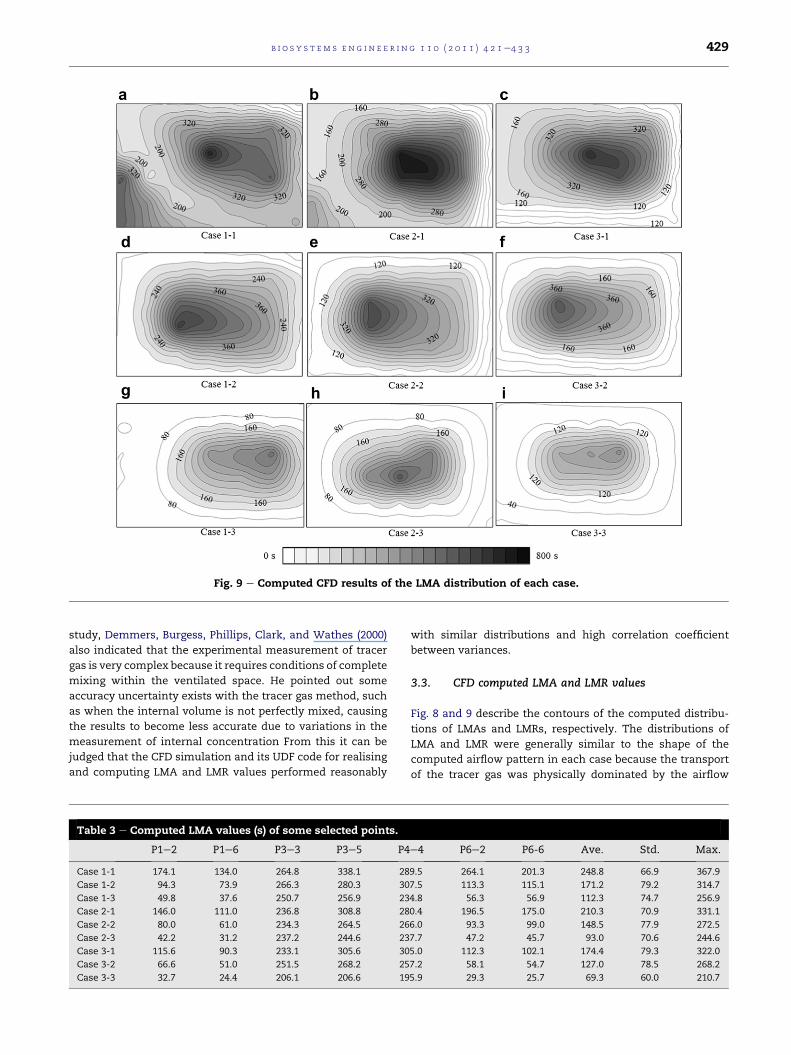
Fig. 9 e Computed CFD results of the LMA distribution of each case.
b i o s y s t em s e ng i n e e r i n g 1 1 0 ( 2 0 1 1 ) 4 2 1e4 3 3 429
study, Demmers, Burgess, Phillips, Clark, and Wathes (2000)
also indicated that the experimental measurement of tracer
gas is very complex because it requires conditions of complete
mixing within the ventilated space. He pointed out some
accuracy uncertainty exists with the tracer gas method, such
as when the internal volume is not perfectly mixed, causing
the results to become less accurate due to variations in the
measurement of internal concentration From this it can be
judged that the CFD simulation and its UDF code for realising
and computing LMA and LMR values performed reasonably
Table 3 e Computed LMA values (s) of some selected points.
P1e2 P1e6 P3e3 P3e5 P4
Case 1-1 174.1 134.0 264.8 338.1 28
Case 1-2 94.3 73.9 266.3 280.3 30
Case 1-3 49.8 37.6 250.7 256.9 23
Case 2-1 146.0 111.0 236.8 308.8 28
Case 2-2 80.0 61.0 234.3 264.5 26
Case 2-3 42.2 31.2 237.2 244.6 23
Case 3-1 115.6 90.3 233.1 305.6 30
Case 3-2 66.6 51.0 251.5 268.2 25
Case 3-3 32.7 24.4 206.1 206.6 19
with similar distributions and high correlation coefficient
between variances.
3.3. CFD computed LMA and LMR values
Fig. 8 and 9 describe the contours of the computed distribu-
tions of LMAs and LMRs, respectively. The distributions of
LMA and LMR were generally similar to the shape of the
computed airflow pattern in each case because the transport
of the tracer gas was physically dominated by the airflow
e4 P6e2 P6-6 Ave. Std. Max.
9.5 264.1 201.3 248.8 66.9 367.9
7.5 113.3 115.1 171.2 79.2 314.7
4.8 56.3 56.9 112.3 74.7 256.9
0.4 196.5 175.0 210.3 70.9 331.1
6.0 93.3 99.0 148.5 77.9 272.5
7.7 47.2 45.7 93.0 70.6 244.6
5.0 112.3 102.1 174.4 79.3 322.0
7.2 58.1 54.7 127.0 78.5 268.2
5.9 29.3 25.7 69.3 60.0 210.7
Table 4 e Computed LMR values (s) of some selected points.
P1e2 P1e6 P3e3 P3e5 P4e4 P6e2 P6-6 Ave. Std. Max.
Case 1-1 169.8 102.3 308.9 559.8 393.4 411.1 241.5 302.3 158.0 754.8
Case 1-2 92.5 79.6 533.5 394.8 591.6 94.6 114.8 205.0 155.8 659.1
Case 1-3 46.9 56.1 153.5 436.3 278.3 52.4 69.7 132.5 114.0 498.5
Case 2-1 154.4 71.1 316.4 694.4 727.0 241.2 193.5 262.5 200.8 771.1
Case 2-2 81.5 57.0 609.7 366.1 471.6 88.1 107.8 180.5 155.4 615.7
Case 2-3 49.8 41.9 221.1 457.0 590.7 59.5 68.0 119.9 130.8 590.7
Case 3-1 155.5 84.3 471.7 619.5 480.7 8.5 14.0 200.4 181.8 719.0
Case 3-2 80.1 57.1 587.4 369.0 405.1 2.0 22.0 149.1 144.5 587.4
Case 3-3 45.7 39.8 321.4 418.9 261.8 0.5 31.6 90.5 98.7 418.9
Table 6 e Computed AER (s) according to the age-of-airvalues.
DesignedAER
Nominaltime constant (s)
CFDcomputed AER
b i o s y s t em s e n g i n e e r i n g 1 1 0 ( 2 0 1 1 ) 4 2 1e4 3 3430
pattern. The values of LMA for Case 1-1 were significantly
greater than for the other cases at every point. This was
because fresh air flowed from the inlet straight through the
upper side wall by the “short-circuiting” phenomenon, which
meant that the main air stream had limited influence on the
internal airflow. This situation decreased the contribution of
the fresh air from the inlet to the flow pattern and resulted in
the formation of stagnant air inside the structure. Compared
to Cases 2-3 and 3-3, the overall values of LMA of Case 1-3,
with the same inlet conditions, were relatively larger because
of short-circuiting. As mentioned above, the LMR values for
Case 1-1 were also significantly greater than those for the
other cases at every point. This obviously showed that the
distribution ability of the fresh air and its potential to elimi-
nate contaminants inside the structure was very poor. The
distributions of LMAs and LMRs showed that the results were
almost similar to shape of the airflow pattern in each case.
However, when the AERwas 2.0, the distributions of LMAs and
LMRs were very similar to each other. These situations arise
because the airflow which formed the internal part of the
simulation domain flowed straight and around the right wall,
producing relatively strong circulating flows. Based on the
qualitative visualisation results of the LMA and LMR distri-
butions, it was concluded that the ventilation efficiencies of
Cases 2 and 3 were superior to that of the Case 1 series;
however, when the AER was 2.0, the results were similar.
Tables 3 and 4 show the quantitative values of the
computed LMAs and LMRs of some selected points in the
corners andmiddle of the simulation structure respectively. It
was found that the LMA and LMR of the areas containing an
eddy were generally greater than those of the other sections
because the air trapped in the eddy disturbed the supply of
fresh air and the emission of contaminant air. This phenom-
enon is shown at representative points 3-3, 3-5, and 4-4 in
Tables 3 and 4. In the case of LMA value at point 3-5, the values
for Case 2-1 and 3-1 were bigger than that for Case 1-1 by 109%
and 110% and in the case of LMR, the values of Case 2-1 and 3-1
were smaller than that of Case 1-1 by 81% and 90%. The
Table 5 e Results of room mean ventilation effectiveness(s) for each case.
Room Mean Age
Case 1-1 252.9 Case 2-1 230.1 Case 3-1 190.4
Case 1-2 170.3 Case 2-2 149.5 Case 3-2 120.8
Case 1-3 99.2 Case 2-3 87.2 Case 3-3 63.5
average LMA and LMR values of each case were smallest for
Case 3-3, indicating that the configuration of Case 3-3 was
superior with regard to fresh air distribution and contaminant
exhaust. The standard deviation values of the LMAs and LMRs
were also found to be minimal in Case 3-3, implying that Case
3-3was also superior in terms of the homogeneity. In contrast,
the standard deviation values of LMAs and LMRs in Case 1-1
were considerably greater than those for the other cases,
illustrating a poor uniformity because of lower efficiency in
terms of fresh air distribution and elimination of contami-
nated air. In all cases, it was concluded that lower LMA and
LMR values were obtained at higher ventilation rates. It is
notable that the LMA and LMR values were lower along the
main air stream, easily observed in the distribution results of
LMAs and LMRs because the areas throughwhich themain air
stream flowed had comparatively greater velocity fields.
3.4. CFD computed RMA and RMR values
The results obtained in the present study are shown in
Table 5. The RMA values in the Case 1 series were relatively
higher than those in the Case 2 and 3 series. It is also observed
that as the ventilation rate increased, the room-mean-
ventilation-effectiveness value was decreased. If the room-
mean-ventilation-effectiveness value is the barometer of the
total distribution ability of fresh air or the ability to eliminate
contaminants, the values of Cases 2-1 and 3-1were superior to
that of Case 1-1 by 108% and 131%, respectively.When the AER
was 1.0, Case 2-2 had a value 114% greater than that of Case 1-
2, and Case 3-2 was 141% greater. When the AER was 2.0, Case
2-3 was 114% and Case 3-3 was 156% greater than was Case 1-
Case 1-1 0.5 122.0 0.49
Case 1-2 1.0 61.6 0.97
Case 1-3 2.0 31.2 1.92
Case 2-1 0.5 119.7 0.50
Case 2-2 1.0 61.7 0.97
Case 2-3 2.0 30.6 1.96
Case 3-1 0.5 117.4 0.51
Case 3-2 1.0 59.6 1.00
Case 3-3 2.0 29.9 2.01
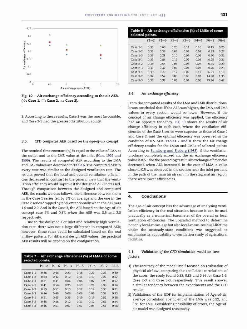
Fig. 10 e Air exchange efficiency according to the air AER.
(>: Case 1, ,: Case 2, 6: Case 3).
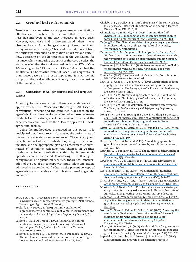
Table 8 e Air exchange efficiencies (%) of LMRs of someselected points.
P1e2 P1e6 P3e3 P3e5 P4e4 P6e2 P6-6
Case 1-1 0.36 0.60 0.20 0.11 0.16 0.15 0.25
Case 1-2 0.33 0.39 0.06 0.08 0.05 0.33 0.27
Case 1-3 0.33 0.28 0.10 0.04 0.06 0.30 0.22
Case 2-1 0.39 0.84 0.19 0.09 0.08 0.25 0.31
Case 2-2 0.38 0.54 0.05 0.08 0.07 0.35 0.29
Case 2-3 0.31 0.37 0.07 0.03 0.03 0.26 0.23
Case 3-1 0.38 0.70 0.12 0.09 0.12 6.91 4.19
Case 3-2 0.37 0.52 0.05 0.08 0.07 14.90 1.35
Case 3-3 0.33 0.38 0.05 0.04 0.06 29.86 0.47
b i o s y s t em s e ng i n e e r i n g 1 1 0 ( 2 0 1 1 ) 4 2 1e4 3 3 431
3. According to these results, Case 3 was the most favourable,
and Case 3-3 had the greatest distribution ability.
3.5. CFD computed AER based on the age-of-air concept
The nominal time constant (sn) is equal to the value of LMA at
the outlet and to the LMR value at the inlet (Han, 1992 and
1999). The results of computed AER according to the LMA
and LMR values are described in Table 6. The computed AER in
every case was similar to the designed ventilation rate. The
results proved that the local and overall ventilation efficien-
cies decreased in contrast to the general view that the venti-
lation efficiencywould improve if the designed AER increased.
Through comparison between the designed and computed
AER, the results were as follows; the difference between them
in the Case 1 series fell by 3% on average and the one in the
Case 2 series dropped by 2.5% exceptionally when the AERwas
1.0 and 2.0. And in the Case 3, the AER based on the Age-of-air
concept rose 2% and 0.5% when the AER was 0.5 and 2.0
respectively.
Due to the designed slot inlet and relatively high ventila-
tion rate, there was not a large difference in computed AER;
however, these rates could be calculated based on the real
airflow pattern. For different design AER values, the practical
AER results will be depend on the configuration.
Table 7 e Air exchange efficiencies (%) of LMAs of someselected points.
P1e2 P1e6 P3e3 P3e5 P4e4 P6e2 P6-6
Case 1-1 0.36 0.46 0.23 0.18 0.21 0.23 0.30
Case 1-2 0.33 0.42 0.12 0.11 0.10 0.27 0.27
Case 1-3 0.31 0.41 0.06 0.06 0.07 0.28 0.27
Case 2-1 0.41 0.54 0.25 0.19 0.21 0.30 0.34
Case 2-2 0.39 0.51 0.13 0.12 0.12 0.33 0.31
Case 2-3 0.36 0.49 0.06 0.06 0.06 0.32 0.33
Case 3-1 0.51 0.65 0.25 0.19 0.19 0.52 0.58
Case 3-2 0.45 0.58 0.12 0.11 0.12 0.51 0.54
Case 3-3 0.46 0.61 0.07 0.07 0.08 0.51 0.58
3.6. Air exchange efficiency
From the computed results of the LMA and LMR distributions,
it was concluded that, if the AERwas higher, the LMA and LMR
values in every section would be lower. However, if the
concept of air change efficiency was applied, the efficiency
had an opposite tendency. Fig. 10 shows the results of air
change efficiency in each case, where the ventilation effi-
ciencies of the Case 3 series were superior to those of Case 1
and Case 2, and the optimal efficiency was observed in the
condition of 0.5 AER. Tables 7 and 8 show the air change
efficiency results for the LMAs and LMRs of selected points.
According to Sandberg and Sjoberg (1983), if the ventilation
produces completely mixed air, the air exchange efficiency
value is 0.5. Like the preceding result, air exchange efficiencies
decreased when AER increased. In the case of LMA, a value
close to 0.5 was observed in the section near the inlet port and
in the path of the main air stream. In the stagnant air region,
there were lower efficiencies.
4. Conclusions
The age-of-air concept has the advantage of analysing venti-
lation efficiency in the real situation because it can be used
practically as a numerical barometer of the overall or local
ventilation efficiencies. The upgraded method to determine
not only local-mean-age but also local-mean-residual-lifetime
under the unsteady-state conditions was suggested to
emphasise its applicability to ventilation study of agricultural
facilities.
4.1. Validation of the CFD simulation model on twofactors
1) The accuracy of the model itself focused on realisation of
physical airflow; comparing the coefficient correlations of
the cases, the study found 0.92, 0.85 and 0.96 for Case 1-3,
Case 2-3 and Case 3-3, respectively. This result showed
a similar tendency between the experiments and the CFD
results.
2) Validations of the UDF for implementation of Age-of-air;
average correlation coefficient of the LMA was 0.92, and
0.91 for LMR. Considering possibility of errors, the Age-of-
air model was designed reasonably.
b i o s y s t em s e n g i n e e r i n g 1 1 0 ( 2 0 1 1 ) 4 2 1e4 3 3432
4.2. Overall and local ventilation analysis
Results of the comparisons among room-mean-ventilation-
effectiveness of each structure showed that the effective-
ness has improved as the AER increased in every case.
However, each case had a different trend when it was
observed locally. Air exchange efficiency of each point and
configuration varied widely. This is interpreted to result from
the airflow pattern such as stagnation of airflow and vortex-
flow. Focussing on the homogeneity of the ventilation, for
instance, when comparing the LMAs of the Case 1 series, the
study revealed that the total standard deviation (STD) of Case
1-3 was higher by 11% than that of Case 1-1 which had the
smallest AER. The total STD value of Case 1-2was higher by 5%
than that of Case 1-3. The result implies that it is worthwhile
computing the local ventilation efficiency of each case besides
of the overall structure.
4.3. Comparison of AER for conventional and computedconcept
According to the case studies, there was a difference of
approximately e3w þ2 %between the designed AER based on
conventional concept and the computed AER based on the
age-of-air. Since these results were limited to the experiments
conducted in this study, it will be necessary to expand the
experimental conditions like the AER or to apply to a full scale
agricultural facility.
Using the methodology introduced in this paper, it is
anticipated that the approach of analysing the performance of
the ventilation system can be enhanced. The efficiency and
expected impact of each ventilation opening on the overall
facilities and the appropriate plan and assessment of elimi-
nation of pollutants reflecting real changes in weather
condition or forced ventilation system by time-schedule
operation can be estimated. Considering the full range of
configuration of agricultural facilities, theoretical consider-
ation of the age-of-air concept with multi-inlets and outlets
will need to be conducted further, as the present concept of
age-of-air is a narrow ideawith simple structure of single inlet
and outlet.
r e f e r e n c e s
Bot G P A. (1983). Greenhouse climate: From physical processes toa dynamic model. Ph.D dissertation. Wagenungen, Netherlands:Wageningen Agricultural University.
Boulard, T., & Draoui, B. (1995). Natural ventilation ofa greenhouse with continuous roof vents: measurements anddata analysis. Journal of Agricultural Engineering Research, 61,27e36.
Boulard T; Baille A; Draoui B (1993). Greenhouse naturalventilation measurements and modeling. InternationalWorkshop on Cooling Systems for Greenhouses, Tel Aviv,AGRIPECH 05e02/03.
Boulard, T., Meneses, J. F., Mermier, M., & Papadakis, G. (1996).The mechanisms involved in the natural ventilation of greenhouses. Agricultural and Forest Meteorology, 79, 61e77.
Chalabi, Z. S., & Bailey, B. J. (1989). Simulation of the energy balancein a greenhouse. Silsoe: AFRC Institute of Engineering Research.Division Note, DN. 1516, 17.
Chanteloup, V., & Mirade, P. S. (2009). Computation fluiddynamics (CFD) modeling of local mean age distribution inforced food plants. Journal of Food Engineering, 90, 90e103.
De Jong T. (1990). Natural ventilation of large multi-span greenhouse.Ph.D dissertation, Wageningen Agricultural University,Wagenungen, Netherlands.
Demmers, T. G. M., Burgess, L. R., Phillips, V. R., Clark, J. A., &Wathes, C. M. (2000). Assessment of techniques for measuringthe ventilation rate using an experimental building section.Journal of Agricultural Engineering Research, 76, 71e81.
Fernandez, J. E., & Bailey, B. J. (1992). Measurement and predictionof greenhouse ventilation rates. Agricultural and ForestMeteorology, 58, 229e245.
Flunet Inc. (2009). Fluent manual. 10, Cavendush, Court Lebanon.,NH 03766: Centerra Resouce Park.
Han, H.-T., Choi, S.-H., & Jang, G.-J. (2001). Distributions of localsupply and exhaust effectiveness according to the roomairflow patterns. The Society of Air-Conditioning and RefrigeratingEngineers of Korea, 13(9).
Han, H.-T. (1992). Numerical approach to calculate ventilationeffectiveness. The Society of Air-Conditioning and RefrigeratingEngineers of Korea, 21(4), 271e281.
Han, H.-T. (1999). On the definition of ventilation effectiveness.The Society of Air-Conditioning and Refrigerating Engineers ofKorea, 28(1), 38e47.
Hong, S.-W., Lee, I.-B., Hwang, H. S., Seo, I.-H., Bitog, J. P., Yoo, J.-I.,et al. (2008). Numerical simulation of ventilation efficiencies ofnaturally ventilated multi-span greenhouse in Korea.Trasaction of ASABE, 51(4), 1417e1432.
Kittas, C., Boulard, T., Mermier, M., & Papadakis, G. (1996). Windinduced air exchange rates in a greenhouse tunnel withcontinuous side openings. Journal of Agricultural EngineeringResearch, 65, 378e449.
Kozai, Sase, T. S., & Nara, M. (1980). A modeling approach togreenhouse environmental control by ventilation. Acta Hort,106, 125e136.
Launder, B., & Spalding, D. (1974). The numerical computation ofturbulent flows. Computer Methods in Applied Mechanics andEngineering, 3(2), 269e289.
Lawrence, W. J. C., & Whittle, R. M. (1960). The climatology ofglasshouses. II. Ventilation. Journal of Agricultural EngineeringResearch, 5, 36e41.
Lee, I.-B., & Short, T. H. (2000). Two dimensional numericalsimulation of natural ventilation in a multi-span greenhouse.American Society of Agricultural Engineers, 43(3), 745e753.
Li, X., Li, D., Yang, X., & Yang, J. (2003). Total air age: an extensionof the air age concept. Building and Environment, 38, 1263e1269.
Morris, L. G., & Neale, F. E. (1954). The infra-red carbon dioxide gasanalyser and its use in glasshouse research. National Institute ofAgricultural Engineering. Tech. Memo. No. 99, Silsoe, 13.
Nederhoff, E. M., Van de Vooren, J., & Udink Ten Cate, A. J. (1985).A practical tracer gas method to determine ventilation ingreenhouses. Journal of Agricultural Engineering Research, 31,309e319.
Norton, T., Grant, J., Fallon, R., & Sun, D. W. (2009). Assessing theventilation effectiveness of naturally ventilated livestockbuildings under wind dominated conditions usingcomputational fluid dynamics. Journal of BiosystemsEngineering, 103, 78e99.
Okada, M., & Takakura, T. (1973). Guide and data for greenhouseair conditioning. 3. Heat loss due to air infiltration of heatedgreenhouses. Journal of Agricultural Meteorology, 28(4), 223e230.
Papadakis, G., Mermier, M., Meneses, J. F., & Boulard, T. (1996).Measurement and analysis of air exchange reates in

b i o s y s t em s e ng i n e e r i n g 1 1 0 ( 2 0 1 1 ) 4 2 1e4 3 3 433
a greenhouse with continuous roof and side openings. Journalof Agricultural Engineering Research, 63, 219e227.
Sandberg, M., & Sjoberg, M. (1983). The use of moments forassessing air quality in ventilated rooms. Building andEnvironment, 18(4), 181e197.
Sandberg, M. (1981). What is ventilation efficiency. Building andEnvironment, 16(2), 123e135.
Seo, I-H., Lee, I.-B.,Moon,O.-K.,Kim,H.-T.,Hwang,H.-S.,Hong,S-W.,etal. (2009). Improvementof theventilationsystemofanaturallyventilated broiler house in the cold season using computationalsimulations. Biosystems Engineering, 104(2009), 106e117.
Wang, A., Zhang, Y., Sun, Y., &Wang, X. (2008). Experimental studyof ventilation effectiveness and air velocity distribution in anaircraft cabin mockup. Building and Environment, 43, 337e343.