A new solution for automatic microstructures analysis from images based on a backpropagation...
20
A New Solution for Automatic Microstructures Analysis from Images Based on a Backpropagation Artificial Neural Network Victor Hugo C. de Albuquerque 1 *, Paulo C. Cortez 2 , Auzuir R. de Alexandria 3 , João Manuel R. S. Tavares 1 . 1 Instituto de Engenharia Mecânica e Gestão Industrial (INEGI), Faculdade de Engenharia da Universidade do Porto (FEUP), Departamento de Mecânica e Gestão Industrial (DEMEGI), Rua Dr. Roberto Frias, S/N, 4200 - 465 Porto – Portugal. 2 Universidade Federal do Ceará (UFC), Departamento de Engenharia de Teleinformática, Av. Mister Hull, S/N – Pici, CEP 60455-970, Fortaleza – Ceará, Brasil. 3 Centro Federal de Educação Tecnológica do Ceará, Indústria, NSMAT, Av. Treze de Maio, 2081 - Benfica , CEP 60040-531, Fortaleza – Ceará, Brasil.
Transcript of A new solution for automatic microstructures analysis from images based on a backpropagation...
A New Solution for Automatic Microstructures Analysis from Images Based on a Backpropagation Artificial Neural Network
Victor Hugo C de Albuquerque 1 Paulo C Cortez2 Auzuir R de Alexandria3
Joatildeo Manuel R S Tavares1
1Instituto de Engenharia Mecacircnica e Gestatildeo Industrial (INEGI) Faculdade de Engenharia da
Universidade do Porto (FEUP) Departamento de Mecacircnica e Gestatildeo Industrial (DEMEGI) Rua
Dr Roberto Frias SN 4200 - 465 Porto ndash Portugal
2Universidade Federal do Cearaacute (UFC) Departamento de Engenharia de Teleinformaacutetica Av
Mister Hull SN ndash Pici CEP 60455-970 Fortaleza ndash Cearaacute Brasil
3Centro Federal de Educaccedilatildeo Tecnoloacutegica do Cearaacute Induacutestria NSMAT Av Treze de Maio 2081 -
Benfica CEP 60040-531 Fortaleza ndash Cearaacute Brasil
Abstract
This paper presents a new solution to segment and quantify the microstructures from images of
nodular gray and malleable cast irons based on an Artificial Neural Network The neural network
topology used is the multilayer perception and the algorithm chosen for its training was the
backpropagation This solution was applied to 60 samples of cast iron images and results were very
similar to the ones obtained by visual human tests This was better than the information obtained from a
commercial system that is very popular in this area In fact this solution segmented the images of
microstructures materials more efficiently Thus we can conclude that it is a valid and adequate option
for researchers engineers specialists and professionals from materials science field to realize a
microstructure analysis from images faster and automatically
Key words Artificial neural networks Image processing and analysis Image segmentation and
quantification Microstructures Multilayer perception Materials Science
1 Introduction
One of the most challenges in the machines and equipments development is the conception of
systems with intelligent capacities so then they could behave like humans Important advances have
been happening in the Artificial Intelligence area and its biggest objective is the research of new
algorithms and technological solutions that can be used in the development of new systems with
stronger intelligent capacities However this is a very challenging and complex task because there are
a lot of actions that people commonly and naturally do as for example visualizing hearing walking
and talking that are very hard to implement in computational systems
Between all of those actions vision has deserved special attention of the research community
because of the considerable number of existing applications and its great importance in our society [1]
Primarily derived from Artificial Intelligence field Computational Vision became a distinct research
area and its objective is to construct systems and hardware solutions that can be able to perform some
visual information analysis and interpretation which can help humans in the execution of some usual
and important tasks with higher speed and precision [2] This new area uses between others
techniques from Artificial Intelligence Digital Signal Processing and Pattern Recognition [3]
Artificial neural networks are commonly used in Artificial Intelligence Pattern Recognition and
in Material Science fields Particularly they have been used in applications that involve objects
recognition from images with high parallelism degree considerable speed classification and important
capacity to learn from examples [4]
In this work is presented a new solution to quantify the metallic materials microstructures from
images based on a neural network To test our solution we used several images samples of nodular
malleable and gray cast irons These materials have been selected because they are commonly used by
industries as in for example structures of machines lamination cylinders main bodies of valves and
pumps and gear elements Additionally we compared the results obtained using our solution with the
ones resulted using a commercial system widely used in Materials Science area for the same purpose
This paper is organized in the following sections In section two the materials and artificial
neural networks are introduced Afterwards the computational solution developed is described Then
in section four some experimental results and their discussion are presented Finally the main
conclusions are addressed in the paperrsquos last section
2 Materials and Artificial neural networks
The main goal of this work was the development of a new solution to segment and quantify
automatically the constituents of nodular malleable and gray cast irons from images The solution
developed and the cast irons consideration are briefly explained into the following sections
21 Cast Irons
Cast irons are mainly composed by iron and carbon being the percentage of the last one
between 214 and 670 In fact the most cast irons contain between 30 and 45 of carbon [17]
Beside carbon the cast irons present significant silicon contents and therefore some authors as for
example Callister [17] Chiaverini [18] and Raabe et al [19] consider the cast iron as an iron alloy
with carbon and silicon Another cast irons characteristic is associated to the carbonrsquos appearance In
gray cast irons all the carbon is presented practically free with the appearance of lamellar graphite or in
veins while in the white cast iron the carbon presented is arranged in the form of cementite (Fe3C)
[20]
In accordance with the carbon content cast irons can be classified as hypoeutectic eutectics or
hypereutectic When eutectic cast iron is solidified there is the formation of a microstructure with
cementite and austenite globules called ledeburite I Continuing the cooling process below 727 ordmC the
austenite transforms itself into pearlite globules on the cementite forming ledeburite II [21] which
deserved main attention of our work
22 Artificial Neural Networks
Artificial neural networks can be applied to solve many engineering problems like function
approximation and classification as in cases that exist nonlinear relations between the dependent and
independent variables
Nowadays artificial neural networks are being used in Material Sciences for welding control
[25] It can obtain the relations between process parameters and correlations in Charpy impact tests
[26] model alloy elements [27 28] microstructures mechanical steels properties [30] and the
deformation mechanism of titanium alloy in hot forming [31] predict weld parameters in pipeline
welding properties of austempered ductile iron the carbon contents and the grain size of carbon steels
[29] build models to predict the flow stress and microstructures evolution of a hydrogenised titanium
alloy [34]
Many systems of image processing and analysis have been developed using artificial neural
networks This is possible because of their main characteristics like robustness to the presence of noisy
data inside the input images speed execution and their possibility to be parallel implemented Zhang
presents a review that is about the usage of neural networks on several image processing and analysis
tasks [37]
The neural network paradigm is to construct a composed model using considerable number of
neurons being each one a very simple processing unit with a great number of connections between
them The information among the neurons in the network is transmitted through the synaptic weights
Artificial neural networks flexibility and its capacity to learn and to generalize the information are very
attractive and important aspects to justify their choice to solve many complex problems In fact the
generalization associated to the network capacity of learning from a training set of examples and their
ability to supply correct results to input data that was not presented in the training set demonstrates that
this neural network capacity goes further than the easy establishment of relations between inputs and
outputs This way artificial neural networks are capable to extract information not presented in explicit
forms in the training examples considered [35]
Different topologies and algorithms for neural networks can be found In this work it was used
a neural network multilayer perception which is a feed forward neural network type [36] Usually a
multilayer perception network is composed of several layers lined up with neurons Then the input
data is presented into its first layer and is distributed trough the internal hidden layers The last neural
network layer is the output one where the problemrsquos solution can be obtained The input and output
layers can be separated by one or more hidden layers also called intermediate layers In many
applications of neural networks just one hidden layer is considered Beyond this the neurons of a layer
are connected to the immediately neurons so there are not unidirectional communication or connection
among the neurons of the same layer All neural layers are totally connected
For the training of the multilayer perception network we adopted a backpropagation algorithm which
is the most used for this neural network structure
3 Solution Developed
The computational solution developed had as its main objective the microstructures
segmentation and quantification presented in metallographic and microphotography images using a
neural network multilayer perception For this purpose each pixel of the input images is classified
according to the microstructures element (pearlite cemetite graphite martensite) In the same way for
the neural network inputs are considered the R G and B color components of each images pixel each
microstructure element is classified corresponding to an individual output of the neural network
Pseudo colors are used to represent each microstructure segmented in the output images
More specifically the artificial neural network used is composed by 39 neurons distributed in
two layers The neurons distribution along the network layers (topology) corresponds to 3 inputs 30
neurons inside the hidden layer and 9 neurons in the output layer As a consequence it is expected that
nine microstructure types come to be segmented
For the neural network training it is necessary to consider some microstructures pixels in a
representative metallographic image This selection is done manually using the mouse device over that
training image The training algorithm used is the standard backpropagation [16] For each type of
material to be analyzed it is necessary to perform the network training
After this the network can analyze each pixel of an input image and then perform the
microstructuresrsquo segmentation During this phase each pixel of the input image is classified and
counters are used to quantify the microstructures identified
Our solution was implemented using C++ and the environment Builder 6 from Borland in
Microsoft Windows XP platform This new system was tested considering several image samples of
cast irons Some of the results obtained are presented and discussed in the next section
4 Experimental Results and Discussion
To make an experimental test in our new computational system we used several samples of
nodular malleable and gray cast irons Additionally to validate the results obtained a commercial
system commonly used in Materials Science field for the same purpose was also considered Moreover
in metallographic images the nodular cast iron has the morphological graphite well defined and the
quantification method manual was also considered [22] In all images considered in this experiment the
graphite is associated to the black color while the pearlite or ferrite are to the gray color
In Table 1 are shown the results obtained from images of a nodular cast iron using our solution
and the commercial system considered With this we can notice that the results obtained using the two
systems are very similar presenting a minimum difference of 215 and a maximum of 71 for
samples 14 and 9 respectively In addition it is clear that our solution presents an average of graphite
equal to 1209 and of pearlite or ferrite to 8791 and that the commercial system presents 1593
and 8407 respectively being the difference between them of 384
Figures 1a) b) and c) present an original image of a nodular cast iron and the resultant images
from the accomplished segmentation process using the commercial system and ours respectively
These images are the ones that present the greatest difference between the results obtained by the two
systems On the other hand images 1d) e) and f) are the ones that present the minor difference
In face of this we noticed that the segmentation done using our solution is more accurate than
the one obtained using the commercial system because it erroneously segmented and classified as
graphite part of the pearlite or ferrite what not occurred with our solution This fact is the most
important reason for the presented divergence in the results obtained by the two systems
In Table 2 are presented the average results obtained using the manual quantification and the
both computational systems and it can be easily distinguished from the ones that are obtained by these
systems This occurs because the manual quantification tends to be an extremely tedious and fastidious
procedure and consequently propitious to generate errors Furthermore to do the manual
quantification with less than 5 of error it was necessary to analyze 206 points of each material
sample using for that a reticulated mesh with 25 intersections [23] The average results obtained using
the manual quantification was 2413 for graphite and 7587 for ferrite or pearlite
For the gray cast iron it was not possible to do the manual quantification because the graphite
appears in the image samples like ribbings (lodes) However the two computational systems
considered can adequately segment and quantify the constituent of this type of iron as well
In Table 3 are presented the results of the quantification using the two computational systems
on gray cast iron images Considering all materials analyzed these are the most similar results obtained
by the two systems because they present a minimum difference of 01 and a maximum of 644 for
samples 1 and 11 respectively Moreover we can notice that our solution presents an average of
graphite equal to 1028 and of pearlite or ferrite to 8962 and on the other hand the commercial
system presented 1209 and 8791 respectively being the difference between them equal to 171
Figures 2 a) b) and c) presents the original image of the gray cast iron used and the resultant
images of the segmentation done using the commercial system and ours respectively These images are
the ones that present the minor difference between all the results By contrast images of Figures 2 d)
e) and f) are the ones that present the biggest difference
Analyzing the results obtained considering the gray cast iron it can be concluded that the
segmentations done using the two systems are very similar for sample 1 Relatively to sample 11 the
segmentation carried through by visual inspection was very similar to the ones obtained using the
computational systems however the quantification obtained by these systems presents a difference of
644
The results obtained using the two systems on samples of nodular and gray cast iron are very
similar as the associated images have good quality and the material constituents are well defined and
with very distinct gray levels
If the two computational systems are applied on images of malleable cast irons with good
quality the results obtained are also very similar as the graphite presents the same tonality that has in
other irons being just different in its morphology that in this case has an appearance similar to flakes
Thus it was decided to apply our solution and the commercial system in images of malleable cast iron
of low quality in which the ash levels of graphite are very similar to the one of pearlite or ferrite This
permitted the evaluation of the efficiency and efficacy of the two systems when they are used in more
adverse conditions
In Table 4 are presented the quantification results obtained by using our solution and the
commercial system considered on a malleable cast iron These results are the most different for the
studied materials presenting a minimal difference of 355 and a maximum of 1516 for samples 18
and 4 respectively Moreover we noticed that our system presents a medium number of graphite equal
to 1498 and of pearlite or ferrite to 8502 and the commercial system presents 2289 and
7711 respectively being the difference between them of 791
Figures 3 a) b) and c) present an original image of the malleable cast iron and the images
resultant from the segmentation done using the commercial system and ours respectively These
images present the minor difference verified between the two systems On the other hand the images of
Figures 3 d) e) and f) present the major difference
Verifying the results we can notice that the segmentations obtained using the two systems are
considerable distinct from each other on sample 4 The same happens with sample 18 because the
commercial system segments great part of the pearlite or ferrite because of the low quality of the
original input image However this error was not verified when our solution was tested because it
segmented correctly the graphite from the other constituents
From the results obtained by the commercial system considering samples of nodular gray and
in particular malleable casting iron (that its commonly used in Materials Science area) we can verify
its difficulty to segment adequately the graphite when the background of the input image was not
uniform However our system does not present that difficulty and so it is able to get results effectively
even when used in more severe conditions
The proposed solution shows to be a versatile and easy tool to use in automatic segmentation
and quantification of material microstructures from images even when the analyzed images are of low
quality Additionally when compared to the commercial system elected in this work for comparison
and validation purposes our system showed that needs less time for the quantification of the structures
presented in the input images
41 Application on Others Microstructures
Our computational system can also be used successfully in the microstructures analysis of
others metallic materials from images For example in Figure 4a) an original microphotography of an
AISI 1020 steel is showed the black color represents the pearlite grain and the white color the ferrite
The segmentation obtained using our system is shown in Figure 4b) and the green color corresponds to
pearlite grain and yellow color to ferrite As we can verify in these images our system segmented
adequately the pearlite and ferrite
In Figure 5a) an original microphotography of an AISI 1045 steel is showed The black color
represents the pearlite grain and the white color the ferrite grain After the segmentation done using
our system we obtained the image presented in Figure 5b) in which the red color corresponds to
pearlite grain and the black color to ferrite As we can see the proposed solution segmented adequately
this image sample
Another possible important application of our computational system can be found in the
segmentation and quantification of metallic materials inclusions [24] Two examples of the results
obtained by our system in this particular application are presented in Figure 6
5 Conclusions
This paper described a new computational solution based on an artificial neural network that
was applied to segment and quantify the constituents of metallic materials from images
After the several experimental tests done considering different metal samples we can
concluded that the system developed can be successfully used in the Materials Science area to do the
segmentation and quantification of material microstructures from images All those experiments
showed some advantages about using our system The most important ones were the simple and easy
way that it can be used and the less sensitive to noise presented in the input images mainly due to
optic distortions or irregular illumination originated by the image acquisition process
Additionally in this work we compared and validated the results obtained by our system with
the corresponding ones obtained using one commercial system very common in the Materials Science
area From this comparison we could conclude that our system was easier to use better when there was
complex applications conditions and that its results always had better quality and could be obtained
faster
Finally we can conclude that our computational system is suitable to be used by researchers
engineers specialists and others professionals from the Materials Science area as an adequate option to
optimize the segmentation and quantification of microstructures of materials from images obtaining
accurate and fast results
6 Acknowledgments
To Federal Center of Technological Education of Cearaacute - CEFET CE in particular to
Mechanical Testing Laboratory and to Tele-Information Laboratory for the support given during the
accomplishment of this work The authors would like to thank also to CAPES for their financial
support
References
[1] F P C Souza A Susin SIAV ndash An automatic vehicle identification system XIII Brazilian
Conference on Automaacutetica (2000) 1377-1380
[2] B Acha C Serrano Image classification based on color and texture analysis IWISPA 2000
PROGRAM (2000)
[3] FVan Der Heidjen Image based measurement systems object recognition and parameter
estimation England - John Wiley amp Sons Inc 1994
[4] D Plaut S Nowlan G E Hinton Experiments on learning by backpropagation Computer
Science Department Carnegie ndash Mellon University Technical Report CMU-CS (1986) 86-126
[5] H K D H Bhadeshia Neural networks in materials science ISIJ International 39
(1999) 966-979
[6] H K D H Bhadeshia Neural networks and genetic algorithms in materials science and
engineering Tata McGraw-Hill Publishing Company Ltd India 2006
[7] L Miaoquan X Liu A Xiong X Li Microstructural evolution and modelling of the hot
compression of a TC6 titanium alloy Materials Characterization 49 (2003) 203ndash209
[8] L Miaoquan X Liu A Xiong X Li An adaptive prediction model of grain size for the forging of
Ti-6Al-4V alloy based on the fuzzy neural networks Journal of Materials Processing
Technology 123 (2002) 377-381
[9] I Kim Y Jeong C Lee P Yarlagadda Prediction of welding parameters for pipeline welding
using an intelligent system The International Journal of Advanced Manufacturing Technology
22 (2003)
[10] J Kusiak R Kuziak Modelling of microstructure and mechanical properties of steel using the
artificial neural network Journal of Materials Processing Technology 127 (2002) 115 ndash 121
[11] X Li L Miaoquan Microstructure evolution model based on deformation mechanism of titanium
alloy in hot forming Transactions of non ferrous metals society of China 15 (2005) 749-753
[12] R Biernacki J Kozłowski D Myszka M Perzyk Prediction of properties of austempered ductile
iron assisted by artificial neural network Materials Science (Medžiagotyra) 12 (2006) 11-15
[13] A Abdelhay Application of artificial neural networks to predict the carbon content and the grain
size for carbon steels Egyptian Journal of Solids 25 (2002) 229 ndash 243
[14] O Wang J Lai D Sun Artificial neural network models for predicting flow stress and
microstructure evolution of a hydrogenized titanium alloy Key Engineering Materials (2007)
541 ndash 544
[15] T Chow Neural networks and computing World Scientific Pub USA 2007
[16] S Haykin Neural networks a comprehensive foundation Macmillian College Publishing
Company Inc USA 1994
[17] W Callister Materials science and engineering an introduction John Wiley amp Sons Inc USA
2006
[18] V Chiaverini Tratamentos teacutermicos das ligas ferrosas Associaccedilatildeo Brasileira de Metais 2ordf ediccedilatildeo
Satildeo Paulo Brazil 1987
[19] D Raabe F Roters F Freacutedeacuteric Barlat L Chen Continuum scale simulation of engineering
materials Wiley InterScience Newsletter 2005
[20] W Wang Engineering alloys properties and applications Marcel Dekker Inc USA 2007
[21] D Zhang T C Leia Z Zhang J Ouyang The effects of heat treatment on microstructure and
erosion properties of laser surface-clad Ni-base alloy Surface and Coatings Technology 115
(1999) 176 ndash 183
[22] V H C Albuquerque P C Cortez A R Alexandria Image segmentation system for
quantification of microstructures in metals using artificial neural networks Revista Mateacuteria 12
(2007) 394-407
[23] A Seabra Correlaccedilatildeo das propriedades mecacircnicas dos accedilos com a microestrutura Lisboa -
Memoacuteria LNEC nordm 522 1979
[24] V H C Albuquerque C C Silva CRO Moura W M Aguiar JP Farias Effect of base
metal characteristics on the success of welding of the AISI 4140 steel without post welding heat
treatment XXXIV National Welding Congress (2007)
FIGURES
a) b) c)
d) e) f)
Figure 1 Two original images of a nodular cast iron a) and d) Resultant images of the segmentation
done using a common commercial system b) and e) and the corresponding images obtained using our
system c) and f)
a) b) c)
d) e) f) Figure 2 Two original images of a gray cast iron a) and d) Resultant images of the segmentation done
using a common commercial system b) and e) and the corresponding images obtained using our
system c) and f)
a) b) c)
d) e) f)
Figure 3 Two original images of a malleable cast iron a) and d) Resultant images of the segmentation
done using a common commercial system b) and e) and the corresponding images obtained using our
system c) and f)
a) b)
Figure 4 An original image of an AISI 1020 steel a) and the image resultant by segmentation using
our system b)
a) b)
Figure 5 An original image of an AISI 1045 steel a) and the image resultant by segmentation using
our system b)
a) b) c) d)
Figure 6 Two original images of inclusions a) and c) and the corresponding images segmented
by our system b) and d)
TABLES
Table 1 Results obtained using the SVRNA and common commercial systems on samples of nodular cast iron
Nodular cast iron
Samples SVRNA Commercial system
Graphite ()
Pearlite ()
Graphite ()
Pearlite ()
Sample1 1151 8849 1752 8248 Sample 2 1336 8664 1991 8009 Sample 3 1319 8681 1805 8195 Sample 4 1346 8654 1763 8237 Sample 5 1246 8754 1698 8302 Sample 6 1179 8821 1707 8293 Sample 7 1458 8542 1838 8162 Sample 8 1250 850 1779 8221 Sample 9 1402 8598 2112 7888 Sample 10 1330 8670 1812 8188 Sample 11 908 9092 1244 8756 Sample12 925 9075 1185 8815 Sample 13 1156 8844 1435 8565 Sample 14 924 9076 1139 8861 Sample 15 1022 8978 1282 8718 Sample 16 989 9011 1274 8726 Sample17 831 9169 1130 887 Sample 18 766 9234 1003 8997 Sample 19 1466 8534 1137 8863 Sample 20 2173 7827 2777 7223 Average 1209 8791 1593 8407
Table 2 Average results obtained using the manual quantification method SVRNA and common commercial systems on samples of nodular cast iron
Method Graphite () PearliteFerrite () Manual 2413 7587 SVRNA 1209 8791 Commercial system
1593 8407
Table 3 Results obtained using the SVRNA common commercial systems on samples of gray cast iron
Gray cast iron
Samples SVRNA Commercial system
Graphite ()
Pearlite ()
Graphite ()
Pearlite ()
Sample1 1221 8779 1231 8769 Sample2 680 9320 720 9280 Sample3 856 9144 1070 8930 Sample4 680 9320 836 9164 Sample5 803 9197 1096 8904 Sample6 502 9498 691 9309 Sample7 873 9127 1121 8879 Sample8 915 9085 1100 8900 Sample9 790 9210 982 9018 Sample10 667 9333 835 9165 Sample11 4041 5959 4685 5315 Sample12 747 9253 1066 8934 Sample13 983 9017 1277 8723 Sample14 752 9248 1052 8948 Sample15 2169 7831 1540 8460 Sample16 879 9121 970 9030 Sample 17 776 9224 1021 8979 Sample18 677 9323 928 9072 Sample19 764 9028 821 9179 Sample 20 778 9222 1135 8865 Average 1028 8962 1209 8791
Table 4 Results obtained using the SVRNA and common commercial systems on samples of malleable
cast iron Malleable cast iron
Samples SVRNA Commercial system
Graphite ()
Pearlite ()
Graphite ()
Pearlite ()
Sample 1 1895 8105 3165 6835 Sample 2 1571 8429 2448 7552 Sample 3 1496 8504 2846 7154 Sample 4 1400 8600 2916 7084 Sample 5 1516 8484 2408 7592 Sample 6 1607 8393 2111 7889 Sample 7 1911 8089 3055 6945 Sample 8 1922 8078 2758 7242 Sample 9 1564 8436 2389 7611 Sample 10 1764 8236 3123 6877 Sample 11 1184 8816 1823 8177 Sample 12 1204 8796 2112 7888 Sample 13 1372 8628 2262 7738 Sample 14 1406 8594 2224 7776 Sample 15 1183 8817 1715 8285 Sample 16 1140 8860 1616 8384 Sample 17 1130 8870 1783 8217 Sample 18 1068 8932 1423 8577 Sample 19 2105 7895 1439 8561 Sample 20 1527 8473 2163 7837 Average 1498 8502 2289 7711
- introduction
- Materials and Artificial neural networks
- 4 Experimental results and Discussion
- 5 Conclusions
- 6 Acknowledgments
-
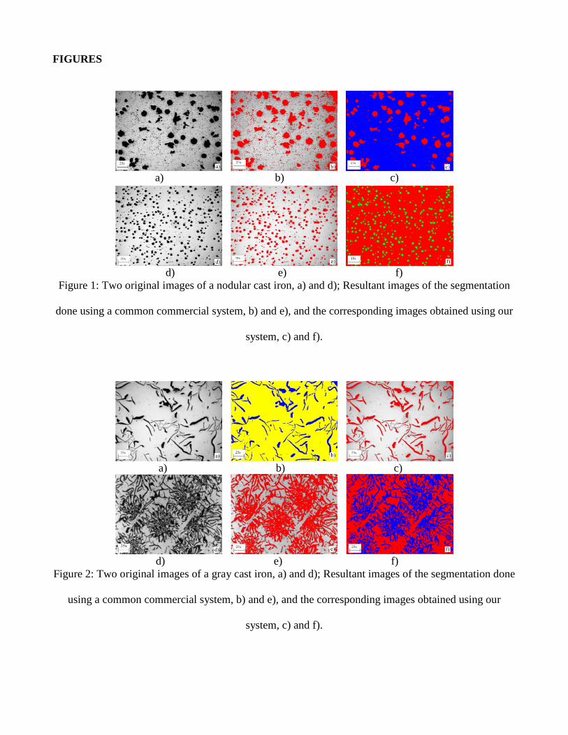
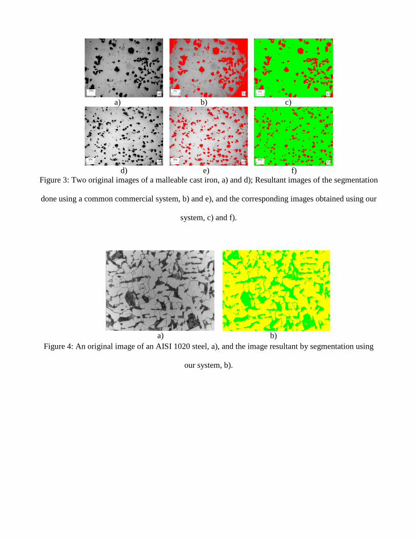
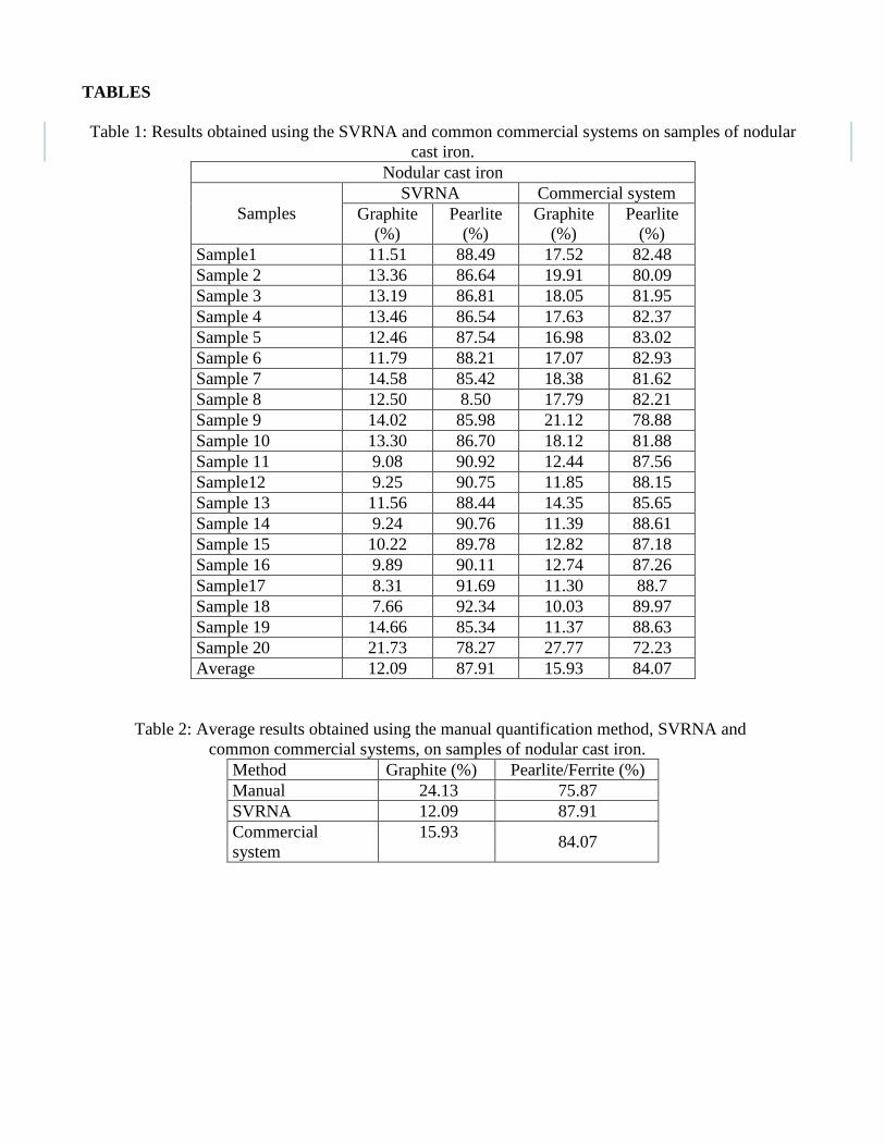
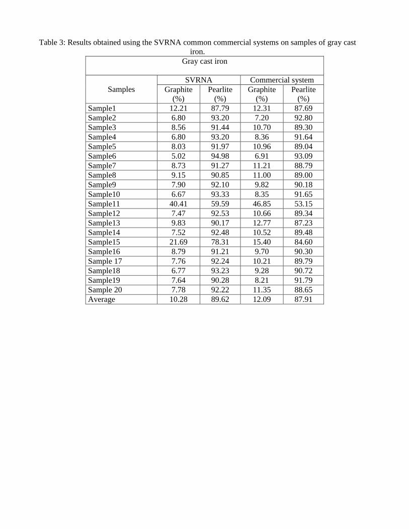
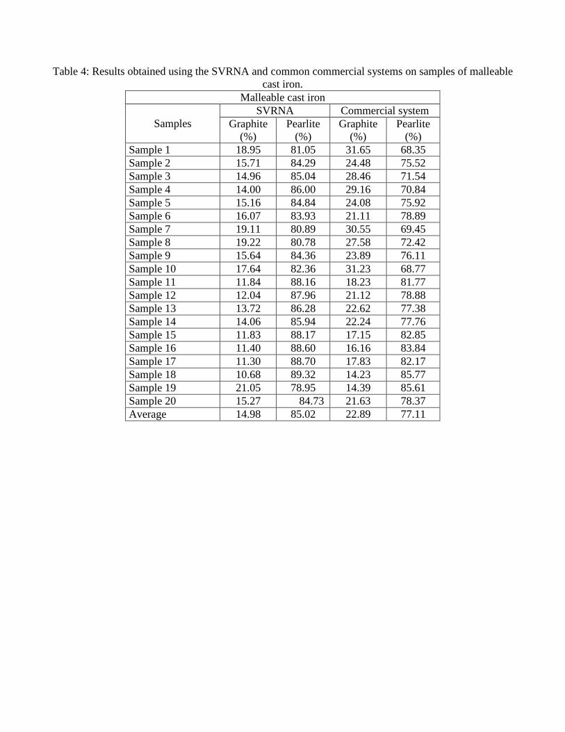