A new microcomputer-based laboratory version of the Ru ¨ chardt experimentfor measuring the ratio gÄCp ÕCv in air

Giacomo Torzoa) and Giorgio DelfittoIstituto Nazionale per la Fisica della Materia, Unita` di Padova, Padova, Italyand Dipartimento di Fisica, Universita` di Padova, Padova, Italy

Barbara PecoriDipartimento di Fisica, Universita` di Bologna, Bologna, Italy

Pietro ScatturinDipartimento di Fisica, Universita` di Padova, Padova, Italy

~Received 10 January 2001; accepted 10 June 2001!

We describe a new version of the Ru¨chardt experiment in which we record the time evolution oftemperature, pressure, and volume oscillating around an equilibrium value. We use a portablemicrocomputer-based laboratory made of a graphic calculator, an interface, two commercial sensors~sonar and barometric sensor!, and a homemade temperature sensor. ©2001 American Association of

Physics Teachers.

@DOI: 10.1119/1.1405505#

orimnee

erresthlimiladph

hita’’

et it i

he‘aie-

hffionla

o

-e

thetally

fullns

glethe

we

onwethe

ec.intheors

a

eory

sti-,

i-n-ex-

I. INTRODUCTION

Experimental investigations of thermodynamic transfmations at the introductory level have always been very lited because of the difficulties in performing simple, but coceptually relevant, lab experiments. Low-cost and usfriendly data acquisition systems have opened npossibilities in this field.

First the possibility of easily collecting measures of thmodynamic variables versus time, at high acquisition fquency with virtually no limits on the number of sampleallows a detailed description of what goes on duringinvestigated transformation. This may have important impcations for student learning. A description of the phenoenon in terms of relevant variables versus time, more simto their spontaneous description,1 can be the first step towarmastering the time-independent description of the samenomenon in terms of equilibrium states.

Second the possibility of easy data reduction allows tnew description to be quickly obtained from experimendata, actually providing the students with a different ‘‘viewof the same experiment.

The present paper is aimed at offering an easy and chway to perform a famous and important experiment thausually only described in textbooks, and rarely carried outhe laboratory: the Ru¨chardt experiment2 where the ratiog5Cp /Cv of the specific heats of air is calculated from tperiod of the oscillations of a sphere supported by an ‘spring.’’ The Ruchardt oscillations are indeed always dscribed asadiabatic transformations in textbooks.3 Are theyreally adiabatic?

A paper published in this Journal4 reported an interestingeffect that shows up when performing this experiment witlarge buffer volume: a sudden drop of the damping coecient and of the oscillation frequency, when the oscillatiamplitude falls below a threshold value. The authors expby a theoretical analysis based on the measured volumecillations that this effect marks a transition from aquasiadia-batic to quasi-isothermalregime.

More recently a second paper5 described a modified version of the same experiment where pressure is also m

1205 Am. J. Phys.69 ~11!, November 2001 http://ojps.aip.or

---r-w

--

,e--r

e-

sl

apsn

r

a-

ins-

a-

sured, and where the volume changesDV can be related tothe corresponding pressure changesDP, allowing an inde-pendent measurement ofg from the slope of theDP vs DVplot. These authors report that under ordinary conditionstransformation in air isalmostadiabatic and that the slighdeparture from adiabatic conditions does not substantiaffect the measured value of theg coefficient.

Here we describe a completely new setup that offers adescription of the thermodynamic transformation by meaof simultaneous measurements of volume, pressure, andtem-peratureoscillations. The students may perform, on a sinset of data, an analysis that proves that in this experimentadiabatic regime is well approximated.

In Sec. II we briefly describe the original Ru¨chardt methodand the approximations on which it is based. In Sec. IIIdescribe both a first microcomputer-based laboratory~MBL !version of the Ru¨chardt apparatus and an improved versidesigned to be easily used in a classroom. In Sec. IVdiscuss the experimental results and we try to answerquestion about ‘‘adiabatic versus isothermal regime.’’ In SV we illustrate the didactical value of this experiment; andSec. VI we draw some conclusions on the advantages oftechnology used in this experiment. Details on the sensused are presented in the Appendix.

II. THE RU CHARDT DEVICE FOR MEASURING g

Adiabatic transformations of a perfect gas, assumingreversible6 process, obey the Poisson equation

PVg5const, ~1!

where the coefficientg is the ratiocp /cv between the con-stant pressure and the constant volume specific heats. Thpredicts forg the valueg5112/j , wherej is the number ofdegrees of freedom of the particles constituting the invegated gas. For air, a mixture of mainly diatomic gasesj55 ~3 translational and 2 rotational degrees of freedom! andthereforeg57/551.4.

Let us now describe the Ru¨chardt method and the approxmations on which it is based. In the original version it ivolved a series of reversible adiabatic compressions and

1205g/ajp/ © 2001 American Association of Physics Teachers

o-d

tht

isi-

w

tn:

re

al

s-

e

ure,

heal-

ol-ted

isin

ges

g

n,sure-

for-ions

by

theto a-ricTFE

sh-

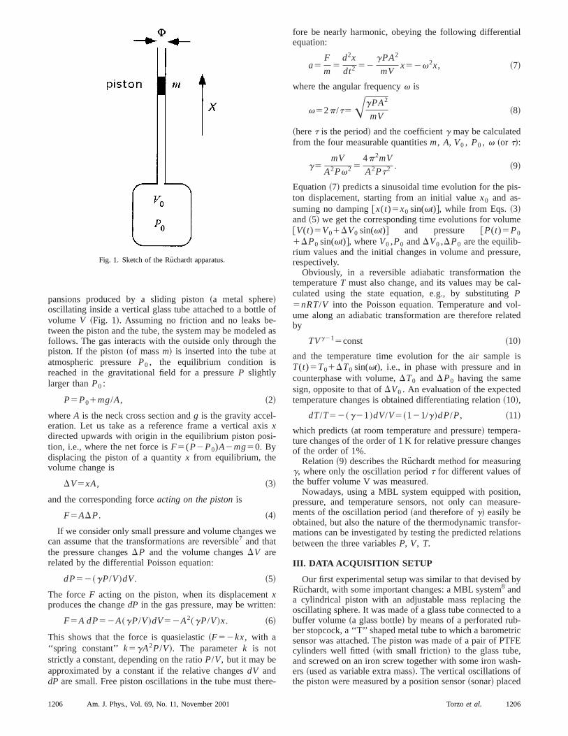
pansions produced by a sliding piston~a metal sphere!oscillating inside a vertical glass tube attached to a bottlevolume V ~Fig. 1!. Assuming no friction and no leaks between the piston and the tube, the system may be modelefollows. The gas interacts with the outside only throughpiston. If the piston~of massm! is inserted into the tube aatmospheric pressureP0 , the equilibrium condition isreached in the gravitational field for a pressureP slightlylarger thanP0 :

P5P01mg/A, ~2!

whereA is the neck cross section andg is the gravity accel-eration. Let us take as a reference frame a vertical axxdirected upwards with origin in the equilibrium piston postion, i.e., where the net force isF5(P2P0)A2mg50. Bydisplacing the piston of a quantityx from equilibrium, thevolume change is

DV5xA, ~3!

and the corresponding forceacting on the pistonis

F5ADP. ~4!

If we consider only small pressure and volume changescan assume that the transformations are reversible7 and thatthe pressure changesDP and the volume changesDV arerelated by the differential Poisson equation:

dP52~gP/V!dV. ~5!

The forceF acting on the piston, when its displacemenxproduces the changedP in the gas pressure, may be writte

F5A dP52A~gP/V!dV52A2~gP/V!x. ~6!

This shows that the force is quasielastic~F52kx, with a‘‘spring constant’’ k5gA2P/V!. The parameterk is notstrictly a constant, depending on the ratioP/V, but it may beapproximated by a constant if the relative changesdV anddP are small. Free piston oscillations in the tube must the

Fig. 1. Sketch of the Ru¨chardt apparatus.

1206 Am. J. Phys., Vol. 69, No. 11, November 2001

f

ase

e

-

fore be nearly harmonic, obeying the following differentiequation:

a5F

m5

d2x

dt252

gPA2

mVx52v2x, ~7!

where the angular frequencyv is

v52p/t5AgPA2

mV~8!

~heret is the period! and the coefficientg may be calculatedfrom the four measurable quantitiesm, A, V0 , P0 , v ~or t!:

g5mV

A2Pv2 54p2mV

A2Pt2 . ~9!

Equation~7! predicts a sinusoidal time evolution for the piton displacement, starting from an initial valuex0 and as-suming no damping@x(t)5x0 sin(vt)#, while from Eqs.~3!and~5! we get the corresponding time evolutions for volum@V(t)5V01DV0 sin(vt)# and pressure @P(t)5P0

1DP0 sin(vt)#, whereV0 ,P0 andDV0 ,DP0 are the equilib-rium values and the initial changes in volume and pressrespectively.

Obviously, in a reversible adiabatic transformation ttemperatureT must also change, and its values may be cculated using the state equation, e.g., by substitutingP5nRT/V into the Poisson equation. Temperature and vume along an adiabatic transformation are therefore relaby

TVg215const ~10!

and the temperature time evolution for the air sampleT(t)5T01DT0 sin(vt), i.e., in phase with pressure andcounterphase with volume,DT0 and DP0 having the samesign, opposite to that ofDV0 . An evaluation of the expectedtemperature changes is obtained differentiating relation~10!,

dT/T52~g21!dV/V5~121/g!dP/P, ~11!

which predicts~at room temperature and pressure! tempera-ture changes of the order of 1 K for relative pressure chanof the order of 1%.

Relation~9! describes the Ru¨chardt method for measuring, where only the oscillation periodt for different values ofthe buffer volume V was measured.

Nowadays, using a MBL system equipped with positiopressure, and temperature sensors, not only can meaments of the oscillation period~and therefore ofg! easily beobtained, but also the nature of the thermodynamic transmations can be investigated by testing the predicted relatbetween the three variablesP, V, T.

III. DATA ACQUISITION SETUP

Our first experimental setup was similar to that devisedRuchardt, with some important changes: a MBL system8 anda cylindrical piston with an adjustable mass replacingoscillating sphere. It was made of a glass tube connectedbuffer volume~a glass bottle! by means of a perforated rubber stopcock, a ‘‘T’’ shaped metal tube to which a barometsensor was attached. The piston was made of a pair of Pcylinders well fitted~with small friction! to the glass tube,and screwed on an iron screw together with some iron waers~used as variable extra mass!. The vertical oscillations ofthe piston were measured by a position sensor~sonar! placed

1206Torzoet al.

we

sesllan

aFisb

inteocoi

akia

erle

urre

-

col-. Ineri-s ais-ons

p.’’lk

one,nerin aethe

di-

in-

esf a

vicebe

at the top of the glass tube. The temperature changesmeasured by a tungsten filament from a broken lamp9 readby a simple amplifying circuit~see the Appendix!. An advan-tage over the original Ru¨chardt design was offered by the uof a variable mass piston allowing different measurementg to be obtained with the same buffer volume. The oscition period was measured by using the ‘‘trace’’ mode on aof the pressure, temperature, position versus time plots.10

This first experimental setup is sketched in Fig. 2, andexample of the measurements it can provide is shown in3. The piston displacements and gas pressure changerecorded in real time, and the plots are immediately availafor the students’ analysis. Figure 3, as well as the followones reporting experimental results, are exact copies ofgraphic calculator screen, where the students may us‘‘running cross-mark’’ to see the coordinates of each pointthe displayed curve. The scale of the axes may be dedufrom the position of the cross-mark and the shown valuesits coordinates. Because perfect sealing is incompatible wlow friction between piston and tube, some air always lethrough the plug, and therefore one must hold the piston wan external applied force, for instance, with a strong permnent magnet interacting with the iron screw and washWhen the magnet is displaced from the tube the piston isfree.

This device was able to provide a rather good measment ofg : In Table I we report some period values measuwith a buffer volumeV5(2.160.02) 1023 m3, a tube diam-eterF5(1.160.02)1022 m, and different values of the piston massm. The calculated values ofg, agree within 4%with the expected value for air (g51.4).

Fig. 2. The first experimental setup.

Fig. 3. Piston displacement and pressure change vs time.

1207 Am. J. Phys., Vol. 69, No. 11, November 2001

re

of-y

ng.areleghe

afedf

thsth-

s:ft

e-d

However when this low-cost version of the classic Ru¨cha-rdt apparatus was presented to high-school teachers, welected comments that led us to design a modified versionfact, it does not seem to be suitable for classroom expment. The long and thin glass tube is brittle and it needcomplicated stand-up system; the low-friction leak-tight pton is not easily homemade; moreover complex operatiare required for changing the oscillating mass.

Therefore we designed a completely new setup11 avoidingboth the glass tube and the piston by using a ‘‘breast-pumThe breast-pump12 is a device, used to drain human mifrom the breast, made of an inner glass tube~with one widerend that is normally pressed against the breast! and an outerglass tube with a closed end that slides outside the inneracting as a ‘‘reversed syringe.’’ The outer surface of the intube is sand-blasted and carefully shaped in order to obtaleak-tight sealing, still offering low friction. Therefore thouter tube may be well used as the oscillating piston forRuchardt experiment.

Figure 4 shows a diagram of this setup: the effectiveameter of the piston is now the inner diameterF528 mm ofthe outer tube, whose mass is 76 g. This may be easilycreased by loading it with a suitable mass~we used brasstubes of various length and inner diameter of 30 mm!. Also,positioning the sonar above the oscillating piston becomeasier in this setup: We may simply attach it at the edge otable using the vise shipped with it, because the whole deis much shorter than in the previous version and it mayplaced on the ground without any supporting stand.

Table I. Measured values of period for different values of piston mass.

m ~g! t ~s! m/t2 g

12.6 0.90 0.0156 1.4113.5 0.93 0.0155 1.4014.5 0.95 0.0160 1.4515.5 1.00 0.0155 1.4016.7 1.05 0.0151 1.37

Fig. 4. Experimental setup with breast-pump and details.

1207Torzoet al.

bntermt

s,

en

alope

soma

lac

7

p

are.

atheictedalls.wehase

dueas

ure

hosents

f-ex-

d-actd ityin a

.

IV. EXPERIMENTAL RESULTS

A typical set of the experimental results that may be otained using the second version of our apparatus is showFig. 5. It is worth noting that a larger number of compleoscillations may be recorded, and that the leaking of aistrongly reduced~the piston oscillates around an equilibriuposition that drifts much less during the whole experimen!.The data shown in Fig. 5 were taken withV5(2.3760.02)31023 m3, m50.147 kg, and the measured period13 was t50.50560.005 s, givingg51.3960.05. Pressure changeare measured in atmospheres, temperature changes in Kpiston displacements in meters. The velocityv and the ac-celerationa of the piston are automatically computed whusing the sonar, as incremental ratiosv i5(xi 112xi 21)/Dtandai5(v i 112v i 21)/Dt. This allows the students to drawplot of the acceleration versus displacement whose sgives immediatelyv2. This is shown in Fig. 6, where thbest fitting line has the slope215263 s22, to be comparedwith the expected value2v252A2gP/mV52154 s22.

The g value may alternatively be calculated from Eq.~5!~which may be written asdP/P52gdV/V!, i.e., from theslope of the measured relative changes in pressure versumeasured relative changes in volume. This requires sdata handling that can be easily performed within the spresheet that is built into the graphic calculator. The volumchanges are calculated from the measured piston dispments and the known value of the piston cross sectionA5pF2/4. The result of this procedure is shown in Fig.where the slope of the fitting line is21.4 ~for pressurechanges up to 0.7% corresponding to volume changes u0.5%!.

Fig. 5. Time graphs of pressure changes~a! and temperature changes~b! ofthe gas, and of displacement~c! and acceleration~d! of the piston.

Fig. 6. Piston acceleration vs displacement from equilibrium position

1208 Am. J. Phys., Vol. 69, No. 11, November 2001

-in

is

and

e

thee

d-ee-

,

to

Because in our apparatus the temperature oscillationsalso measured, a third value ofg may be calculated using Eq~11!: dT/T52(g21)dV/V. The slope of the curve in thedT/T vs dV/V plot in Fig. 8 is20.18, corresponding to thesmaller valueg51.18. This result might be interpreted asproof of nonadiabaticity of the transformation, becausemeasured temperature changes are smaller than the predvalues, suggesting strong heat transfer to the vessel wBut if we observe that the data in Fig. 8 lie on an ellipse,deduce that the measured temperature signal suffers a plag with respect to the measured volume signal. This isto the finite heat capacity of the lamp filament, which actsa low-pass filter for the signal induced by the temperatchanges of the surrounding gas.

The measured temperature changes are about half of tpredicted by Eq.~11!. Therefore temperature measuremeare here intrinsically unable to answer the question as tohowmuch the transformation departs from anideal adiabaticprocess.14 They can only prove that we arefar from an iso-thermal regime. But temperature measurements may still ofer an interesting consideration in this experiment, asplained in the following section.

V. DISCUSSION OF THE EDUCATIONAL VALUE OFTHE EXPERIMENT

The use of MBL in this experiment introduces some avantages for the introductory-level laboratory course. In fthe students who are not advanced in calculus might findifficult to derive Eq.~5! from Eq. ~1!. These students mathen use the data stored in the graphic calculator to obta

Fig. 7. Relative pressure changes vs relative volume changes.

Fig. 8. Relative temperature changes vs relative volume changes.

1208Torzoet al.

m

ehea

fesu

oectina

ch

n

u

o

s-ic

-

ge

rgy

ir

d.

b-erim-the

heomaxi-

n,ould

eom-temricustd inr-

ss-use

se ofthe

n-

l-y

the

l-

ea-f 2

ld

time graph of the productPV and of the productPVg versustime, in order to investigate the nature of the gas transfortion ~Fig. 9!. We calculated values of therelative changesofthese products with respect to their average values~i.e.,PV/^PV&21 andPVg/^PVg&21! to make the comparisoneasier. The productPV shows large oscillations, while thproductPVg remains substantially constant, proving that tPoisson equation~1! is more appropriate than the isothermequation for describing the observed transformation.

An equivalent procedure that also does not require difential calculus is the power-law best fit of the pressure vervolume data, that gives for the exponent theg value. Figure10 shows the fitting line and the experimental data plottedtwo different scales: the first one expanded in order to chthe goodness of fit, the second one zoomed-out to includeorigin. These plots clearly show how small is the regionthe P–V plane that is covered by the adiabatic transformtion. The usual plots in the textbooks in fact show muwider regions, corresponding to larger relative changespressure and volume. But it is clear that in the real world ocannot performreversibleandadiabatic transformations in-volving such large relative changes, because one mchoose betweenfast quasiadiabatic, orslow quasireversibleprocesses. The two together cannot be achieved with gapproximation.

The results of the Ru¨chardt experiment may also be dicussed as an example of direct conversion of mechanwork into internal energy.

From the values of specific heat (Cv'1 J/g) and density(r'1.331023 g/cm3) of air, found in the textbooks, the stu

Fig. 9. Time graphs of the relative changes ofPV ~line! andPVg ~crosses!.

Fig. 10. Plot of pressure vs volume; best fitting curve:P50.000 21 V21.4.

1209 Am. J. Phys., Vol. 69, No. 11, November 2001

a-

l

r-s

nk

he

-

ine

st

od

al

dents may estimate the changeDE of the internal energy ofa volumeV of air corresponding to a temperature chanDT:

DE5rVCvDT. ~12!

This change may then be compared with the potential enechanges ~gravitational DUg5mgDx or elastic DUe

5kDx2/2! of the system made of the piston and the ‘‘aspring’’ with elastic constantk5A2(gP/V). The result(DE@DUg) is usually surprising for the students, who finit difficult to explain where this extra energy comes fromThis is obviously due to taking into account only the susystem made of the piston and the ‘‘air-spring.’’ The teachmay use this common misunderstanding to discuss theportant difference between closed and open systems. Inopen system made of the piston and the ‘‘air-spring,’’ ttotal energy is not conserved. In fact if the piston starts frrest, mechanical energy conservation must give for the mmum elongationDx, where the piston has zero velocity:

DUg5mgDx5DUe5E kx dx5A2~gP/2V!Dx2. ~13!

Equation~13! was indeed first used by Rinkel15 to measurethe ratio of specific heats asg52mgV/(A2PDx). Thechoice of the maximum elongation simplifies the calculatiobecause for a generic value of the displacement one shalso take into account the kinetic energyEc51/2mv2 of thepiston.

However, to explain the ‘‘extra energy’’ transferred to thair corresponding to the increased temperature during a cpression, one must take into account the whole syspiston-air~including the air above the piston at atmosphepressureP0!. In the whole system, the energy change mbe equal to the total work done on the air volume enclosethe reservoir. Here the work is not simply the work peformed by thenet force F5mg2kx applied to the piston.This in fact should be exactly zero, as in any vertical maspring oscillator when damping can be neglected, becathe increase of elastic energy compensates the decreagravitational energy. For example, with the data of Fig. 5,students would calculate, for a full oscillation~displacement62 cm!, a temperature riseDT'0.5 K, corresponding, forthe 2.37 g of air contained in the volumeV, to an energyincreaseDE5rVCvDT'1.3 J On the other hand the potetial energy terms are much smaller. For example, withm5147 g, and a total displacementDx'4 cm, we getDUg

52DUe'20.06 J, which is 20 times smaller than the caculated DE. Moreover, if we calculate the total work btaking into account thetotal gravitational force, which in-cludes that due to the mass of the air column abovepiston, i.e., F5AP01mg, we obtain W5FDx5(P0A1mg)Dx'2.5 J, which is about twice the value of the caculated increase of the internal energyDE. If we assume thatthe total energy must be conserved, we deduce that the msured temperature changes must be about a factor osmaller than the real ones~see the discussion about Fig. 8!.With this assumption the slope in the plot of Fig. 8 shouchange to20.36, which gives from Eq.~11! the valueg51.36, which differs only 4% from the theoretical value.

1209Torzoet al.

ateo

/opitivt

insotimstiosvacs

ainhe

e

unayg

e

tuerr

toi

en

b

nr

Wfi

r-

encill

ghat

ig-

n-

ghalue

i,in

–pro-

of

sed

oesmeena

ol-

pro-ion

ic

g

is

VI. CONCLUSIONS

We have shown that with a simple and cheap apparone may perform an interesting thermodynamic experimto illustrate the quasiadiabatic transformation of a massgas, which usually requires very skilled operators andvery expensive and fragile apparatuses. An interesting asof this experimental setup is the use of a fast and sensthermometer to measure the gas temperature oscillationsare made possible by a system where energy exchangetween the working gas and the ambient is substantiallyhibited. By using volume, pressure, and temperature senthe system is completely characterized by the measuredevolution of all three thermodynamic variables. This allowdetailed discussion of various aspects of the transformato be carried out. The description of the phenomenon afunction of time may be enlightening for students who hadifficulties in building a description in terms of state equtions ~time invariant!, such as those typical of thermostatifound in textbooks, and the features of the experiment mbe usefully exploited for discussing the energy balancesystem whose description involves both mechanical and tmodynamical quantities.

APPENDIX

1. The pressure sensor calibration

The Vernier barometric sensor~BAR-DIN! can easilymeasure pressure changes of the order of 1022 atm, and it isfairly linear. Therefore it may be calibrated as follows. Wconnect a known volume~500-cm3 bottle! to the probe andto a graduated syringe by means of the threefold valve splied with the probe. We seal the air volume in the bottle asyringe at room pressure, with the syringe piston halfwthen we measure the pressure reached after decreasinvolume by a known amount~e.g., DV5210 cm3, corre-sponding toP51.02 atm!, and then by increasing the volum~e.g., DV5110 cm3, corresponding toP50.98 atm!. Thiscalibration procedure is normally well understood by sdents who have previously performed the isothermal expment to test Boyle’s law, with a calibrated Vernier pressuprobe~PS-DIN!.

2. The volumetric sensor

The changes of the air volume sealed by the sliding pisare indirectly measured by the piston displacements fromequilibrium position, which are detected by the position ssor~sonar, MD-CBL whose sensibility is about 1 mm! placedjust above the glass tube. Calibration is simply obtainedmeasuring the inner diameter of the outer cylinder.

3. The temperature sensor

Commercial thermoresistive sensors or thermistors canbe used to measure gas temperature changes of the ordeK at fast acquisition rates~20 Hz!: Their surface to volumeratio is too low to achieve reliable quick measurements.therefore used a homemade sensor made of a tungstenment from a~7-W, 220-V! lamp, whose glass bulb was peforated. At room temperature the filament resistanceR isabout 500V, and the tungsten thermal coefficient isa5(dR/R)/dT'0.005 K21. This requires the use of a bridgconfiguration to make detectable the small resistachanges produced by small-amplitude temperature osc

1210 Am. J. Phys., Vol. 69, No. 11, November 2001

usntfr

ecte

hatbe--rs,e

ana

e-

yar-

p-d;the

-i-e

nts-

y

otof 1

ela-

ea-

tions (DT,1 K). We therefore inserted the filamentF ~Fig.11! into a Wheatstone bridge, powered by the CBL throuthe operational amplifier IC1a, whose inputs are blocked2.5 V by the Voltage Reference IC2. The bridge output snal, preamplified by IC1b with gainG5101, is fed to theanalog input port of CBL. The filament is biased by a costant current of 0.76 mA through the resistorR0 ~3.3 kV!.The thermometer sensitivity isdV/dT5GaIR'0.19 V/K,with a temperature resolution~given by the 5 mV voltageresolution of the interface ADC converter! better than 0.03K.

The 1-kV potentiometer P1 allows one to perform a roubridge balance, which depends on the exact resistance vof the filament used and the 100-V potentiometer P may beused for a fine adjustment of the output voltageV0 , whichdepends on the room temperatureT0 ~e.g., setting V0

52.5 V, the midpoint of the 0–5 V range!. The sensor cali-bration is therefore provided by the equation:T2T05(V2V0)/GaIR'5.3(V22.5) K.

a!Electronic mail: torzo@padova.infm.it1N. Grimellini Tomasini, B. Pecori Balandi, J. L. A. Pacca, and A. Villan‘‘Understanding conservation laws in mechanics: Students’ difficultieslearning about collisions,’’ Sci. Educ.77 ~2!, 169–189~1993!.

2E. Ruchardt, ‘‘Eine Einfache Methode zur Bestimmung vonCp /Cv , ’’Phys. Z.30, 58–59~1929!.

3See, for example, M. W. Zemansky,Heat and Thermodynamics~McGraw–Hill, New York, 1957!, Chap. 5, where the method of KatzWoods–Leverton to account for the departures from ideal adiabaticcess is also mentioned.

4O. L. de Lange and J. Pierrus, ‘‘Measurement of bulk moduli and ratiospecific heats of gases using Ru¨chardt’s experiment,’’ Am. J. Phys.68,265–270~2000!.

5G. D. Severn and T. Steffensen, ‘‘A simple extension of Ru¨chardt’s methodfor measuring the ratio of specific heats of air using microcomputer-balaboratory sensors,’’ Am. J. Phys.69, 387–389~2001!.

6A reversible thermodynamic transformation is an ideal process that gthrough equilibrium states, and therefore the time derivatives of voluand pressure must be small. This may be approximated with phenominvolving large changes ofP and V by proceeding slowly or with fastphenomena by involving smallP andV changes.

7This assumption is justified for oscillations with relative pressure and vume changes of a few percent, for frequencies up to a few Hz.

8We used a TI-89 hand-held graphic calculator and the CBL interfaceduced by Texas Instruments, with barometric probe BAR-DIN and MotDetector, MD-CBL, produced by Vernier Software, Portland, OR.

9G. De Bernardis, M. De Paz, M. Pilo, and G. Sonnino, ‘‘Thermodynamexperiments on gases with a computer on-line,’’ Phys. Educ.24, 222–229~1994!.

10Values measured for the periodt should be corrected for the dampineffect, e.g., assuming a viscous drag,t'tmis$12(l/p)2%, wherel is thelogarithmic decrement of the oscillation amplitude, ort'tmis$12(t/2pt0)2%, where t0 is the oscillation decay time. In our case th

Fig. 11. Diagram of the sensor circuitry: IC1a5IC1b5(1/2)LT1013,IC25TL431.

1210Torzoet al.

tal

re

alu

ausevenera-actmentss

effect is negligible@with t'1 s andt0'3 s, we get (t/2pt0)2'0.3%#.11This apparatus was patented and is now produced by MAD, I

~grolive@tin.it!.12We used a model produced by Chicco®, Italy.13The period was measured by selecting, on the graphic calculator sc

displaying the distance versus time plot, the coordinates of maximumminimum elongation. The half-period was then derived as the mean vof the selected time intervals.

THE MYSTERY OF COM

‘‘Yes, yes, I know all that just as well as youabout the whole thing? I don’t quite know howlike that you begin with ordinary solid numbesomething else that’s quite tangible at any ratenumbers. But these two lots of real numbers aIsn’t that like a bridge where the piles are therthe middle, and yet one crosses it just as suresort of operation makes me feel a bit giddy, asI really feel is so uncanny is the force that lieson you that in the end you land safely on the

Spoken by To¨rless in Robert Musil,Young To¨rless~The New1964!, p. 90.

1211 Am. J. Phys., Vol. 69, No. 11, November 2001

y

enore

14Purely adiabatic transformations are not physically achievable becthermal coupling of the gas with the vessel walls is always present. Eif they were achievable, it would not be possible to measure the tempture in a transformation which is strictly adiabatic: Some energy in fmust be transferred to or drained from the system to obtain a measureof its temperature. Therefore the definition ‘‘adiabatic’’ for a real proceshould always be taken as meaning ‘‘approximately adiabatic.’’

15R. Rinkel, ‘‘Die Bestimmung vonCp /Cv , ’’ Phys. Z. 30, 805 ~1929!.

PLEX NUMBERS

do. But isn’t there still something very odd indeedto put it. Look, think of it like this: in a calculationrs, representing measures of length or weight or, they’re real numbers. And at the end you have realre connected by something that simply doesn’t exist.e only at the beginning and at the end, with none inly and safely as if the whole of it were there? That

if it led part of the way God knows where. But whatin a problem like that, which keeps such a firm holdother side.’’

American Library of World Literature, Inc., New York, NY,

1211Torzoet al.