A new method for generating families of continuous distributions

METRON (2013) 71:63–79DOI 10.1007/s40300-013-0007-y

A new method for generating families of continuousdistributions

Ayman Alzaatreh · Carl Lee · Felix Famoye

Received: 9 March 2011 / Accepted: 16 February 2013 / Published online: 10 April 2013© Sapienza Università di Roma 2013

Abstract In this paper, a new method is proposed for generating families of continuousdistributions. A random variable X , “the transformer”, is used to transform another randomvariable T , “the transformed”. The resulting family, the T -X family of distributions, hasa connection with the hazard functions and each generated distribution is considered as aweighted hazard function of the random variable X . Many new distributions, which aremembers of the family, are presented. Several known continuous distributions are found tobe special cases of the new distributions.

Keywords Hazard function · Pearson system · Beta-family · Generalized distribution ·Entropy · Shannon entropy

1 Introduction

Statistical distributions are commonly applied to describe real world phenomena. Due to theusefulness of statistical distributions, their theory is widely studied and new distributions aredeveloped. The interest in developing more flexible statistical distributions remains strongin statistics profession. Many generalized classes of distributions have been developed andapplied to describe various phenomena. A common feature of these generalized distributionsis that they have more parameters. Johnson et al. [19] stated that the use of four-parameterdistributions should be sufficient for most practical purposes. According to these authors, atleast three parameters are needed but they doubted any noticeable improvement arising fromincluding a fifth or sixth parameter.

A. AlzaatrehDepartment of Mathematics and Statistics, Austin Peay State University,Clarksville, TN 37044, USA

C. Lee · F. Famoye (B)Department of Mathematics, Central Michigan University,Mount Pleasant, MI 48859, USAe-mail: [email protected]

123

64 A. Alzaatreh et al.

The Pearson system of continuous distributions, as developed by Pearson [31], is a systemfor which every probability density function (p.d.f.) f (x) satisfies a differential equation ofthe form

1

f (x)

d f (x)

dx= a + x

b0 + b1x + b2x2 , (1.1)

where a, b0, b1, and b2 are the parameters (see Johnson et al. [19, Chapter 12]). The shape ofthe function f (x) depends on the parameters. The different shapes of the distribution wereclassified by Pearson into a number of types. The different types correspond to the differentforms of solution to (1.1). The form of solution of (1.1) depends on the roots of the equationb0 +b1x +b2x2 = 0. An example is when b1 = b2 = 0, which led to the normal distributionand this is not assigned to a particular type. For a detailed discussion of the various types,see Chapter 12 of Johnson et al. [19]

Burr [5] presented a system of continuous distributions which can take on a wide varietyof shapes. The system of distributions satisfy the differential equation

d F = F(1 − F)g(x)dx, (1.2)

where 0 ≤ F ≤ 1 and g(x) is a non-negative function over x . Burr [5] gave 12 solutions tothe equation in (1.2) and these correspond to the choices of g(x). See Fry [15] and Johnsonet al. [19] for a list of Burr Types I–XII distributions.

Johnson [18] proposed a system for generating distributions using normalization trans-formation with the general form

Z = γ + δ f

(x − ξ

λ

), (1.3)

where f (.) is the transformation function, Z is a standardized normal random variable, γand δ are shape parameters, λ is a scale parameter and ξ is a location parameter. Withoutloss of generality, Johnson assumed that δ and λ are positive. He proposed three transfor-mation functions and defined the lognormal family, the bounded system of distributions andunbounded system of distributions. These families of distributions cover many commonlyused distributions such as normal, log-normal, gamma, beta, exponential distributions, andothers. For more discussions, see Johnson et al. [19, p.33].

Tukey [37] proposed lambda distribution, which was generalized by Ramberg andSchmeiser [32,33] and Ramberg et al. [34] as the so-called generalized lambda distribu-tions (GLD). This family of distributions is defined in terms of percentile function

Q(y) = Q(y; λ1, λ2, λ3, λ4) = λ1 + yλ3 − (1 − y)λ4

λ2, where 0 ≤ y ≤ 1. (1.4)

The parameters λ1 and λ2 are, respectively, location and scale parameters, while λ3 and λ4

determine the skewness and kurtosis. The corresponding p.d.f. is given by

f (x) = λ2

λ3 yλ3−1 + λ4(1 − y)λ4−1 , with x = Q(y). (1.5)

The existence of a valid p.d.f. requires the condition that λ3 yλ3−1 + λ4(1 − y)λ4−1 has thesame sign for all y in [0, 1] and that λ2 takes the same sign. Freimer et al. [14] discussedthe similarity and differences between the Pearson’s system and the GLD. They pointed outthat Pearson’s family does not include logistic distribution, while GLD does not cover all

123

Families of continuous distributions 65

skewness and kurtosis values. An extended GLD was proposed by Karian and Dudewicz [23]that consists of both GLD and generalized beta distribution defined as

f (x) ={

(x−β1)β3 (β1+β2−x)β4

B(β3+1, β4+1)β(β3+β4+1)2

, for β1 ≤ x ≤ β1 + β2

0, otherwise,(1.6)

where B(., .) is the complete beta function. For detailed discussion about the GLD andextended GLD, see Karian and Dudewicz [23].

Azzalini [4] introduced the skew normal family of distributions. Suppose X and Y areindependent random variables, each with a p.d.f. that is symmetric about zero. For any λ,

0.5 = P(X − λY < 0) =∞∫

−∞fY (y)FX (λy)dy. (1.7)

Thus, 2 fY (y)FX (λy) is a probability density function. If X and Y are each standard normal,N (0, 1), then the skew-normal family of distributions has the p.d.f.

2ϕ(x)�(λx), (1.8)

where ϕ(x) and �(x) are N (0, 1) p.d.f. and cumulative distribution function respectively.The distribution in (1.8) is characterized by a single parameter λ. Location and scale para-meters can be added to the distribution in (1.8) by using the translation Y = μ + σ X . Forskew normal distribution and other systems of continuous distributions, see Johnson et al.[19, Chapter 12].

Eugene et al. [10] used the beta distribution as a generator to develop the so-called family ofbeta-generated distributions. The cumulative distribution function (c.d.f.) of a beta-generatedrandom variable X is defined as

G(x) =F(x)∫0

b(t)dt, (1.9)

where b(t) is the p.d.f. of the beta random variable and F(x) is the c.d.f. of any randomvariable. The p.d.f. corresponding to the beta-generated distribution in (1.9) is given by

g(x) = 1

B(α, β)f (x)Fα−1(x)(1 − F(x))β−1. (1.10)

This family of distributions is a generalization of the distributions of order statistics for therandom variable X with c.d.f. F(x) as pointed out by Eugene et al. [10] and Jones [21].Since the paper by Eugene et al. [10], many beta-generated distributions have been studiedin the literature including the beta-Gumbel distribution by Nadarajah and Kotz [29], beta-exponential distribution by Nadarajah and Kotz [30], beta-Weibull distribution by Famoyeet al. [12], beta-gamma by distribution Kong et al. [24], beta-Pareto by distribution Akinseteet al. [1], and others.

Recently, Jones [22] and Cordeiro and de Castro [6] extended the beta-generated familyof distributions by replacing the beta distribution in (1.9) with the Kumaraswamy distri-bution, b(t) = αβxα−1(1 − xα)β−1, x ∈ (0, 1), Kumaraswamy [25]. The p.d.f. of theKumaraswamy generalized distributions (K W -G) is given by

g(x) = αβ f (x)Fα−1(x)(1 − Fα(x))β−1. (1.11)

123


Several generalized distributions from (1.11) have been studied in the literature including theKumaraswamy Weibull distribution by Cordeiro et al. [7], the Kumaraswamy generalizedgamma distribution by de Castro et al. [9], and the Kumaraswamy generalized half-normaldistribution by Cordeiro et al. [8].

Ferreira and Steel [13] introduced a method to generate skewed distributions throughinverse probability integral transformations. According to Ferreira and Steel [13], a distri-bution G is said to be a skewed version of the symmetric distribution F , generated by theskewing mechanism P , if its p.d.f. is of the form

g(y|F, P) = f (y)p(F(y)). (1.12)

Note that the p.d.f. (1.12) is a weighted function of f (.)with the weight p(F(.)). The skewednormal family in (1.8) is a special case of this family. By relaxing the assumption F(.) beingsymmetric, the beta-generated family (1.10) is a special case of (1.12).

This article presents yet another technique to generate families of continuous probabil-ity distributions. The article is organized as follows: Sect. 2 presents a new technique forgenerating families of continuous distributions. Section 3 gives examples of classes of gen-eralized families developed using the technique in Sect. 2. The paper ends with a summaryand conclusion in Sect. 4.

2 Method for generating families of continuous probability distributions

The beta-generated family of distributions in (1.10) and the K W -G family of distributionsin (1.11) are generated by using distributions with support between 0 and 1 as the generator.The beta random variable and the K W random variable lie between 0 and 1, so is the c.d.f.F(x) of any other random variable. The limitation of using a generator with support lyingbetween 0 and 1 raises an interesting question: ‘Can we use other distributions with differentsupport as the generator to derive different classes of distributions?’ This section will addressthis question and introduce a new technique to derive families of distributions by using anyp.d.f. as a generator.

Let r(t) be the p.d.f. of a random variable T ∈ [a, b], for −∞ ≤ a < b ≤ ∞. LetW (F(x)) be a function of the c.d.f. F(x) of any random variable X so that W (F(x)) satisfiesthe following conditions:

W (F(x)) ∈ [a, b]W (F(x)) is differentiable and monotonically non-decreasingW (F(x)) → a as x → −∞ and W (F(x)) → b as x → ∞.

⎫⎬⎭ (2.1)

A method for generating new families of distribution is presented in the following definition.

Definition Let X be a random variable with p.d.f. f (x) and c.d.f. F(x). Let T be a continuousrandom variable with p.d.f. r(t) defined on [a, b]. The c.d.f. of a new family of distributionsis defined as

G(x) =W (F(x))∫

a

r(t)dt, (2.2)

where W (F(x)) satisfies the conditions in (2.1). The c.d.f. G(x) in (2.2) can be written asG(x) = R{W (F(x))}, where R(t) is the c.d.f. of the random variable T . The correspondingp.d.f. associated with (2.2) is

123


g(x) ={

d

dxW (F(x))

}r{W (F(x))}. (2.3)

Note that:

• The c.d.f. in (2.2) is a composite function of (R.W.F)(x).• The p.d.f. r(t) in (2.2) is “transformed” into a new c.d.f. G(x) through the function,

W (F(x)), which acts as a “transformer”. Hence, we shall refer to the distribution g(x)in (2.3) as transformed from random variable T through the transformer random variableX and call it “Transformed-Transformer” or “T -X” distribution.

• The random variable X may be discrete and in such a case, G(x) is the c.d.f. of a familyof discrete distributions.

• The distribution (1.12) introduced by Ferreira and Steel [13] is a special case of (2.3) bydefining W (F(x)) = F(x) and r(.) plays the same role as the weight function.

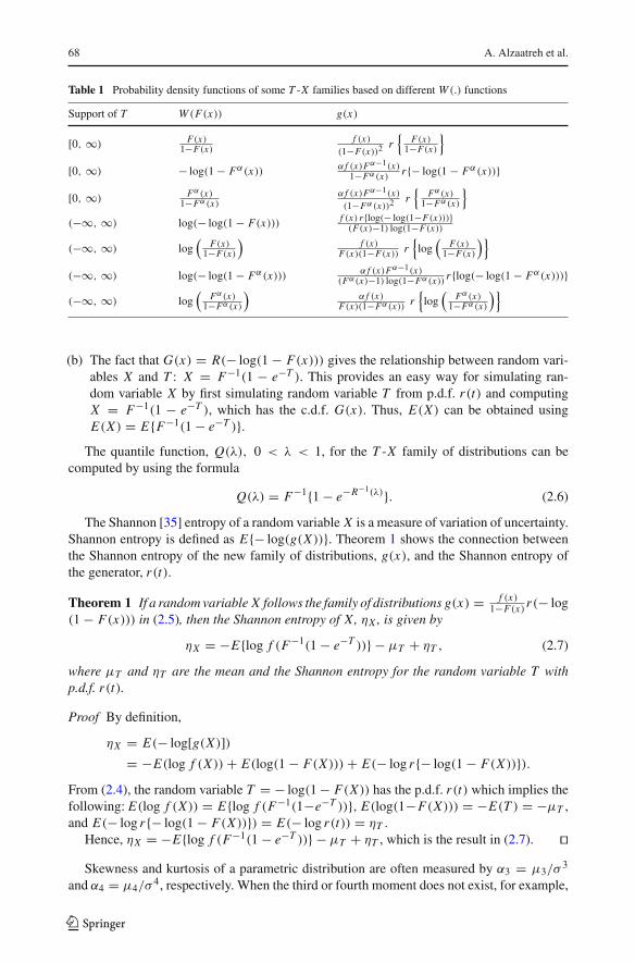
Different W (F(x)) will give a new family of distributions. The definition of W (F(x))depends on the support of the random variable T . The following are some examples of W (.).

1. When the support of T is bounded: Without loss of generality, we assume the supportof T is [0, 1]. Distributions for such T include uniform (0, 1), beta, Kumaraswamy andother types of generalized beta distributions. W (F(x)) can be defined as F(x) or Fα(x).This is the beta-generated family of distributions which have been well studied duringthe recent decade.

2. When the support of T is [a, ∞), a ≥ 0: Without loss of generality, we assume a =0.W (F(x)) can be defined as − log(1 − F(x)), F(x)/(1 − F(x)),− log(1 − Fα(x)),and Fα(x)/(1 − Fα(x)), where α > 0.

3. When the support of T is (−∞, ∞): W (F(x)) can be defined as log[− log(1 −F(x))], log[F(x)/(1 − F(x))], log[− log(1 − Fα(x))], and log[Fα(x)/(1 − Fα(x))].

By using the W (F(x)) = − log(1 − F(x)) in the second example, the G(x) in (2.2) is ac.d.f. of the new family of distributions which is given by

G(x) =−log(1−F(x))∫

0

r(t)dt = R{− log(1 − F(x))}, (2.4)

where R(t) is the c.d.f. of the random variable T . The corresponding p.d.f. associated with(2.4) is

g(x) = f (x)

1 − F(x)r(− log(1 − F(x))) = h(x) r(− log(1 − F(x))), (2.5)

where h(x) is the hazard function for the random variable X with the c.d.f. F(x).The corresponding families of distributions generated from the other W (.) functions men-

tioned in examples 2 and 3 are given in Table 1.In the remainder of this article, we will focus on the case when T has the support [0, ∞)

and W (F(x)) = − log(1 − F(x)). For simplicity, we will use the name T -X family ofdistributions for the new family of distributions in (2.5).

Some remarks on the family of distributions defined in (2.5):

(a) The p.d.f. in (2.5) can be written as g(x) = h(x)r(H(x)) and the corresponding c.d.f.is G(x) = R(− log(1 − F(x))) = R(H(x)), where h(x) and H(x) are hazard andcumulative hazard functions of the random variable X with c.d.f. F(x). Hence, thisfamily of distributions can be considered as a family of distributions arising from aweighted hazard function.

123


Table 1 Probability density functions of some T -X families based on different W (.) functions

Support of T W (F(x)) g(x)

[0, ∞)F(x)

1−F(x)f (x)

(1−F(x))2r{

F(x)1−F(x)

}

[0, ∞) − log(1 − Fα(x)) α f (x)Fα−1(x)1−Fα(x) r{− log(1 − Fα(x))}

[0, ∞)Fα(x)

1−Fα(x)α f (x)Fα−1(x)(1−Fα(x))2

r{

Fα(x)1−Fα(x)

}

(−∞, ∞) log(− log(1 − F(x))) f (x) r{log(− log(1−F(x)))}(F(x)−1) log(1−F(x))

(−∞, ∞) log(

F(x)1−F(x)

)f (x)

F(x)(1−F(x)) r{

log(

F(x)1−F(x)

)}

(−∞, ∞) log(− log(1 − Fα(x))) α f (x)Fα−1(x)(Fα(x)−1) log(1−Fα(x)) r{log(− log(1 − Fα(x)))}

(−∞, ∞) log(

Fα(x)1−Fα(x)

)α f (x)

F(x)(1−Fα(x)) r{

log(

Fα(x)1−Fα(x)

)}

(b) The fact that G(x) = R(− log(1 − F(x))) gives the relationship between random vari-ables X and T : X = F−1(1 − e−T ). This provides an easy way for simulating ran-dom variable X by first simulating random variable T from p.d.f. r(t) and computingX = F−1(1 − e−T ), which has the c.d.f. G(x). Thus, E(X) can be obtained usingE(X) = E{F−1(1 − e−T )}.

The quantile function, Q(λ), 0 < λ < 1, for the T -X family of distributions can becomputed by using the formula

Q(λ) = F−1{1 − e−R−1(λ)}. (2.6)

The Shannon [35] entropy of a random variable X is a measure of variation of uncertainty.Shannon entropy is defined as E{− log(g(X))}. Theorem 1 shows the connection betweenthe Shannon entropy of the new family of distributions, g(x), and the Shannon entropy ofthe generator, r(t).

Theorem 1 If a random variable X follows the family of distributions g(x) = f (x)1−F(x)r(− log

(1 − F(x))) in (2.5), then the Shannon entropy of X, ηX , is given by

ηX = −E{log f (F−1(1 − e−T ))} − μT + ηT , (2.7)

where μT and ηT are the mean and the Shannon entropy for the random variable T withp.d.f. r(t).

Proof By definition,

ηX = E(− log[g(X)])= −E(log f (X))+ E(log(1 − F(X)))+ E(− log r{− log(1 − F(X))}).

From (2.4), the random variable T = − log(1 − F(X)) has the p.d.f. r(t) which implies thefollowing: E(log f (X)) = E{log f (F−1(1−e−T ))}, E(log(1−F(X))) = −E(T ) = −μT ,and E(− log r{− log(1 − F(X))}) = E(− log r(t)) = ηT .

Hence, ηX = −E{log f (F−1(1 − e−T ))} − μT + ηT , which is the result in (2.7). ��Skewness and kurtosis of a parametric distribution are often measured by α3 = μ3/σ

3

and α4 = μ4/σ4, respectively. When the third or fourth moment does not exist, for example,

123


Cauchy, Lévy and Pareto distributions, α3 and α4 cannot be computed. For the T -X family,one may encounter some difficulty in computing the third and fourth moments. Alternativemeasures for skewness and kurtosis, based on quantile functions, are sometimes more appro-priate for such distributions. The measure of skewness S defined by Galton [16] and themeasure of kurtosis K defined by Moors [27] are based on quantile functions and they aredefined as

S = Q(6/8)− 2Q(4/8)+ Q(2/8)

Q(6/8)− Q(2/8), (2.8)

K = Q(7/8)− Q(5/8)+ Q(3/8)− Q(1/8)

Q(6/8)− Q(2/8). (2.9)

Skewness measures the degree of the long tail (towards left or right side). Kurtosis isa measure of the degree of tail heaviness. When the distribution is symmetric, S = 0 andwhen the distribution is right (or left) skewed, S > 0 (or< 0). As K increases, the tail of thedistribution becomes heavier. For the T -X family, Galton’s skewness and Moors’ kurtosis canbe computed by using the quantile function in (2.6) and the appropriate T and X distributions.

3 Some families of T -X distributions with different T distributions

The T -X family of distributions can be further classified into two sub-families: One sub-family has the same X distribution but different T distributions and the other sub-familyhas the same T distribution but different X distributions. For example, by letting T be aWeibull random variable, we generate a sub-family of Weibull-X distributions. By letting Xbe a Weibull random variable, we generate a sub-family of T -Weibull distributions. In thissection, we consider the sub-family with different T distributions. Table 2 gives several suchsub-families with the same X and different T random variables.

In each of the following sub-sections, we discuss the properties of the gamma-X family,beta-exponential-X family, and Weibull-X family.

3.1 Gamma-X family

If a random variable T follows the gamma distribution with parameters α and β, then r(t) =(�(α)βα)−1tα−1e−t/β, t > 0. From (2.5), the p.d.f. of gamma-X family is defined as

g(x) = 1

�(α)βαf (x)(− log(1 − F(x)))α−1(1 − F(x))

1β

−1. (3.1)

By using (2.4) and expressing the c.d.f. of the gamma distribution in terms of the incompletegamma function, R(t) = (1/�(α))γ (α, t/β), where γ (α, t) = ∫ t

0 uα−1e−udu, the c.d.f.of the gamma-X family in (3.1) is G(x) = γ {α,− log(1 − F(x))}/�(α). We will refer todistributions of the form (F(x))c and (1 − F(x))c as, respectively, Exp(F) and Exp(1 − F)family of distributions.

Lemma 1 The Shannon entropy of the gamma-X family of distributions is given by ηX =−E{log f (F−1(1 − e−T ))} + α(1 − β)+ logβ + log�(α)+ (1 − α)ψ(α), where ψ is thedigamma function.

Proof It follows from Theorem 1 by usingμT = αβ and the Shannon entropy for the gammadistribution, which is given by Song [36] as ηT =α+logβ+log�(α)+(1 − α)ψ(α). ��

123


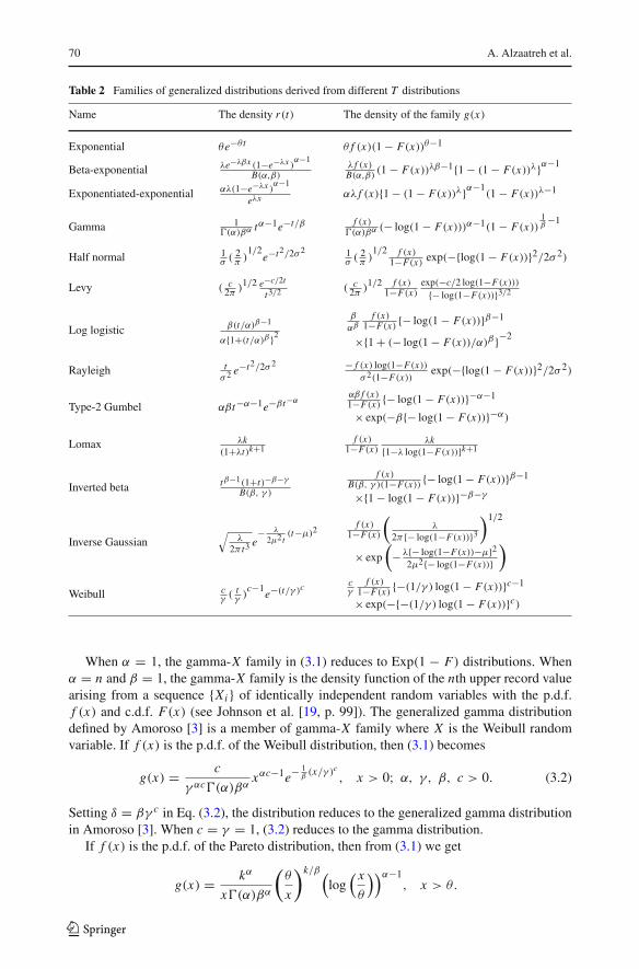
Table 2 Families of generalized distributions derived from different T distributions

Name The density r(t) The density of the family g(x)

Exponential θe−θ t θ f (x)(1 − F(x))θ−1

Beta-exponential λe−λβx (1−e−λx )α−1

B(α,β)λ f (x)B(α,β) (1 − F(x))λβ−1{1 − (1 − F(x))λ}α−1

Exponentiated-exponential αλ(1−e−λx )α−1

eλx αλ f (x){1 − (1 − F(x))λ}α−1(1 − F(x))λ−1

Gamma 1�(α)βα

tα−1e−t/β f (x)�(α)βα

(− log(1 − F(x)))α−1(1 − F(x))1β

−1

Half normal 1σ (

2π )

1/2e−t2/2σ2 1

σ (2π )

1/2 f (x)1−F(x) exp(−{log(1 − F(x))}2/2σ 2)

Levy ( c2π )

1/2 e−c/2t

t3/2 ( c2π )

1/2 f (x)1−F(x)

exp(−c/2 log(1−F(x))){− log(1−F(x))}3/2

Log logistic β(t/α)β−1

α{1+(t/α)β }2

β

αβf (x)

1−F(x) {− log(1 − F(x))}β−1

×{1 + (− log(1 − F(x))/α)β }−2

Rayleigh tσ2 e−t2/2σ2 − f (x) log(1−F(x))

σ2(1−F(x))exp(−{log(1 − F(x))}2/2σ 2)

Type-2 Gumbel αβt−α−1e−βt−ααβ f (x)1−F(x) {− log(1 − F(x))}−α−1

× exp(−β{− log(1 − F(x))}−α)Lomax λk

(1+λt)k+1f (x)

1−F(x)λk

{1−λ log(1−F(x))}k+1

Inverted beta tβ−1(1+t)−β−γB(β, γ )

f (x)B(β, γ )(1−F(x)) {− log(1 − F(x))}β−1

×{1 − log(1 − F(x))}−β−γ

Inverse Gaussian√

λ

2π t3 e− λ

2μ2 t(t−μ)2 f (x)

1−F(x)

(λ

2π{− log(1−F(x))}3

)1/2

× exp

(− λ{− log(1−F(x))−μ}2

2μ2{− log(1−F(x))})

Weibull cγ (

tγ )

c−1e−(t/γ )c cγ

f (x)1−F(x) {−(1/γ ) log(1 − F(x))}c−1

× exp(−{−(1/γ ) log(1 − F(x))}c)

When α = 1, the gamma-X family in (3.1) reduces to Exp(1 − F) distributions. Whenα = n and β = 1, the gamma-X family is the density function of the nth upper record valuearising from a sequence {Xi } of identically independent random variables with the p.d.f.f (x) and c.d.f. F(x) (see Johnson et al. [19, p. 99]). The generalized gamma distributiondefined by Amoroso [3] is a member of gamma-X family where X is the Weibull randomvariable. If f (x) is the p.d.f. of the Weibull distribution, then (3.1) becomes

g(x) = c

γ αc�(α)βαxαc−1e− 1

β(x/γ )c

, x > 0; α, γ, β, c > 0. (3.2)

Setting δ = βγ c in Eq. (3.2), the distribution reduces to the generalized gamma distributionin Amoroso [3]. When c = γ = 1, (3.2) reduces to the gamma distribution.

If f (x) is the p.d.f. of the Pareto distribution, then from (3.1) we get

g(x) = kα

x�(α)βα

(θ

x

)k/β(log

( x

θ

))α−1, x > θ.

123


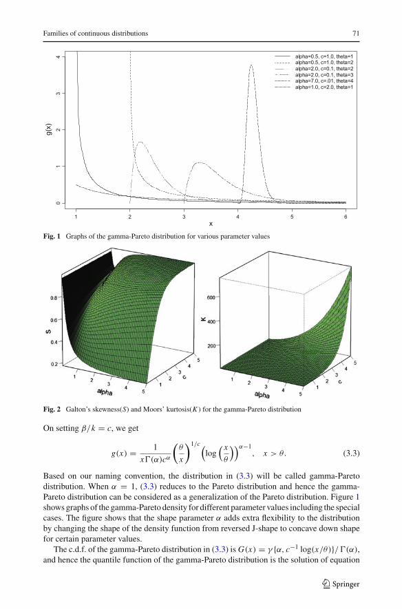
Fig. 1 Graphs of the gamma-Pareto distribution for various parameter values

Fig. 2 Galton’s skewness(S) and Moors’ kurtosis(K ) for the gamma-Pareto distribution

On setting β/k = c, we get

g(x) = 1

x�(α)cα

(θ

x

)1/c(log

( x

θ

))α−1, x > θ. (3.3)

Based on our naming convention, the distribution in (3.3) will be called gamma-Paretodistribution. When α = 1, (3.3) reduces to the Pareto distribution and hence the gamma-Pareto distribution can be considered as a generalization of the Pareto distribution. Figure 1shows graphs of the gamma-Pareto density for different parameter values including the specialcases. The figure shows that the shape parameter α adds extra flexibility to the distributionby changing the shape of the density function from reversed J-shape to concave down shapefor certain parameter values.

The c.d.f. of the gamma-Pareto distribution in (3.3) is G(x) = γ {α, c−1 log(x/θ)}/�(α),and hence the quantile function of the gamma-Pareto distribution is the solution of equation

123


G(x) = p, 0 ≤ p ≤ 1. To investigate the effect of the two shape parameters α and c on thegamma-Pareto density function, Eqs. (2.8) and (2.9) are used to obtain Galton’s skewnessand Moors’ kurtosis. Figure 2 displays the Galton’s skewness and Moors’ kurtosis for thegamma-Pareto distribution in terms of the parameters α and c when θ = 1.

From Fig. 2 and the corresponding data values (not included to save space), the Gal-ton’s skewness is always positive which indicates that the gamma-Pareto distribution is rightskewed. For fixed c ≥ 1, the Galton’s skewness is an increasing function of α. For fixedc < 1, the Galton’s skewness is a decreasing function of α and for fixed α, the Galton’sskewness is an increasing function of c. The Moors’ kurtosis is an increasing function of αand c.

3.2 Beta-exponential-X family

If a random variable T follows the beta-exponential distribution in Nadarajah and Kotz [30],

then r(t) = λ(B(α, β))−1e−λβt (1 − e−λt )α−1

. From (2.5), the p.d.f. of the beta-exponential-X family is defined as

g(x) = λ

B(α, β)f (x)(1 − F(x))λβ−1{1 − (1 − F(x))λ}α−1

. (3.4)

The c.d.f. of (3.4) can be expressed in terms of the incomplete beta function Ix (a, b). Thec.d.f. of the beta-exponential-X family is G(x) = 1 − I(1−F(x))λ (λ(β − 1)+ 1, α).

Lemma 2 The Shannon entropy of the beta-exponential-X family of distributions is givenby

ηX = −E{log f (F−1(1 − e−T ))} + log(λ−1 B(α, β))+ (α + β − 1)ψ(α + β)

−(α − 1)ψ(α)− βψ(β)− [ψ(α + β)− ψ(β)]/λ.

Proof It follows from Theorem 1 by using the mean μT = [ψ(α + β) − ψ(β)]/λ and theShannon entropy ηT = log(λ−1 B(α, β))+ (α + β − 1)ψ(α + β)− (α − 1)ψ(α)− βψ(β)

for the beta-exponential distribution, which are given by Nadarajah and Kotz [30]. ��

Special cases of beta-exponential-X family:

(1) The beta-generated family in (1.10) is a special case of (3.4) when λ = 1. Hence, thefamily of distributions in (3.4) can be used to generate all the distributions belonging tothe beta-generated family.

(2) When α = 1, the beta-exponential-X family reduces to the Exp(1 − F) distributions.When β = 1 and λ = 1, the beta-exponential-X reduces to the Exp(F) distributions.

(3) When β = 1, (3.4) reduces to the exponentiated-exponential-X family with p.d.f.

g(x) = αλ f (x){1 − (1 − F(x))λ}α−1(1 − F(x))λ−1. (3.5)

The c.d.f of (3.5) can be written as G(x) = {1 − (1 − F(x))λ}α .

123


By using D(x) = 1 − F(x) in (3.5), the exponentiated-exponential-X family reduces tothe K W -G family.

If X is the uniform random variable, then from (3.4) the beta-exponential-uniform isdefined as

g(x) = λ

B(α, β)

1

b − a

(b − x

b − a

)λβ−1{

1 −(

b − x

b − a

)λ}α−1

, a < x < b. (3.6)

If we use the transformation y = 1 − x in (3.6) then the distribution reduces to the (i) gener-alized beta distribution of the first kind (McDonald [26]), when b = 1, (ii) beta distributionwhen a = 0 and b = λ = 1, and (iii) Kumaraswamy’s [25] double bounded distributionwhen a = 0 and b = β = 1.

The exponentiated-Weibull distribution defined by Mudholkar et al. [28] is a member ofexponentiated-exponential-X family in (3.5) when X is the Weibull random variable. If f (x)is the p.d.f. of the Weibull distribution, then (3.5) reduces to

g(x) = cλα

γ

(x

γ

)c−1

(1 − e−λ(x/γ )c )α−1e−λ(x/γ )c , x > 0; c, γ, α, λ > 0. (3.7)

Writing δ = λγ c, (3.7) reduces to the exponentiated-Weibull distribution given by Mudholkaret al. [28]. When γ = c = 1, (3.7) reduces to the exponentiated-exponential distributiondefined by Gupta and Kundu [17]. When λ = c = 1, (3.7) reduces to the Weibull distribution.When λ = γ = c = 1, (3.7) reduces to the exponential distribution.

The type I generalized logistic distribution given by Johnson et al. [20, p. 140], is a specialcase of exponentiated-exponential-logistic distribution. If f (x) is the p.d.f. of the standardlogistic distribution then (3.5) reduces to

g(x) = αλe−λx

(1 + e−x )λ+1

(1 − e−λx

(1 + e−x )λ

)α−1

, −∞ < x < ∞, α, λ > 0. (3.8)

When λ = 1, the exponentiated-exponential-logistic distribution in (3.8) reduces to typeI generalized logistic distribution. When α = λ = 1, (3.8) reduces to standard logisticdistribution.

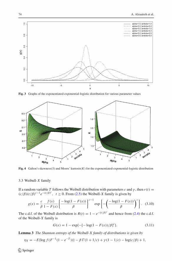
Figure 3 shows graphs of the exponentiated-exponential-logistic density functions fordifferent parameter values including the special cases.

The c.d.f. of the exponentiated-exponential-logistic distribution in equation (3.8) isG(x) = (1 − (1 + ex )−λ)α, and hence the quantile function of the exponentiated-exponential-logistic distribution can be written as

Q(p) = log((1 − p1/α)−1/λ − 1), 0 ≤ p ≤ 1. (3.9)

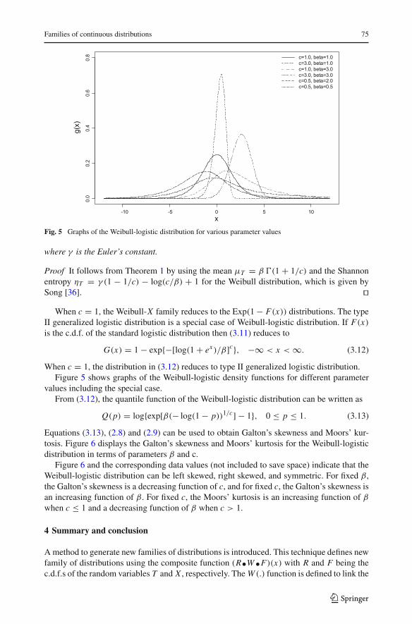
By using (3.9), (2.8) and (2.9), one can obtain the Galton’s skewness and the Moors’ kurtosisfor the exponentiated-exponential-logistic distribution. Figure 4 displays the Galton’s skew-ness and Moors’ kurtosis for the exponentiated-exponential-logistic distribution in terms ofthe parameters α and λ.

From Fig. 4 and the corresponding data values (not included in order to save space),the exponentiated-exponential-logistic distribution can be left skewed, right skewed, andsymmetric. For fixed λ > 1, the Galton’s skewness is an increasing function of α, and forfixed α, the Galton’s skewness is a decreasing function of λ. For fixed α, the Moors’ kurtosisis a decreasing function of λwhen λ > 1, and for fixed λ, the Moors’ kurtosis is a decreasingfunction of α when α > 1.

123


Fig. 3 Graphs of the exponentiated-exponential-logistic distribution for various parameter values

Fig. 4 Galton’s skewness(S) and Moors’ kurtosis(K ) for the exponentiated-exponential-logistic distribution

3.3 Weibull-X family

If a random variable T follows the Weibull distribution with parameters c and γ , then r(t) =(c/β)(t/β)c−1e−(t/β)c , t ≥ 0. From (2.5) the Weibull-X family is given by

g(x) = c

β

f (x)

1 − F(x)

{− log(1 − F(x))

β

}c−1

exp

{−

(− log(1 − F(x))

β

)c}. (3.10)

The c.d.f. of the Weibull distribution is R(t) = 1 − e−(t/β)c and hence from (2.4) the c.d.f.of the Weibull-X family is

G(x) = 1 − exp{−[− log(1 − F(x))/β]c}. (3.11)

Lemma 3 The Shannon entropy of the Weibull-X family of distributions is given by

ηX = −E{log f (F−1(1 − e−T ))} − β �(1 + 1/c)+ γ (1 − 1/c)− log(c/β)+ 1,

123


Fig. 5 Graphs of the Weibull-logistic distribution for various parameter values

where γ is the Euler’s constant.

Proof It follows from Theorem 1 by using the mean μT = β �(1 + 1/c) and the Shannonentropy ηT = γ (1 − 1/c) − log(c/β) + 1 for the Weibull distribution, which is given bySong [36]. ��

When c = 1, the Weibull-X family reduces to the Exp(1 − F(x)) distributions. The typeII generalized logistic distribution is a special case of Weibull-logistic distribution. If F(x)is the c.d.f. of the standard logistic distribution then (3.11) reduces to

G(x) = 1 − exp{−[log(1 + ex )/β]c}, −∞ < x < ∞. (3.12)

When c = 1, the distribution in (3.12) reduces to type II generalized logistic distribution.Figure 5 shows graphs of the Weibull-logistic density functions for different parameter

values including the special case.From (3.12), the quantile function of the Weibull-logistic distribution can be written as

Q(p) = log{exp[β(− log(1 − p))1/c] − 1}, 0 ≤ p ≤ 1. (3.13)

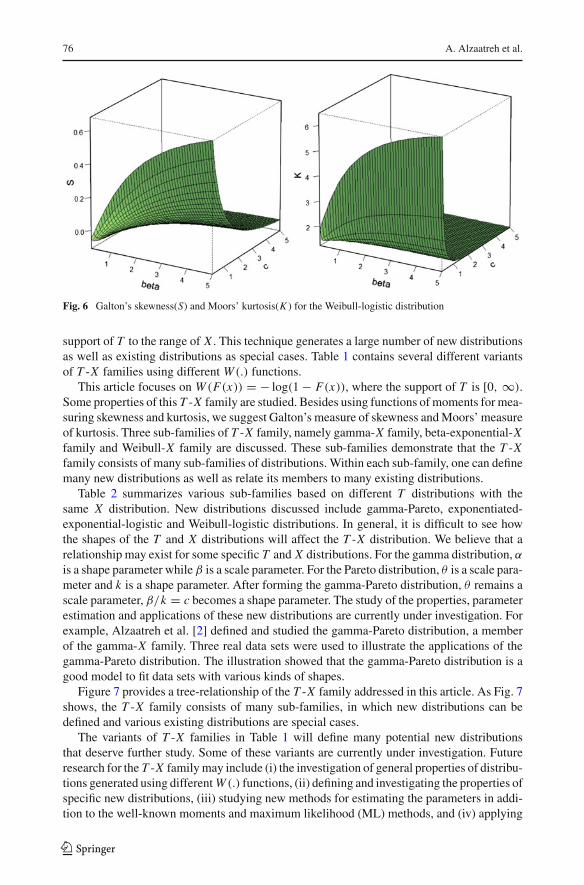
Equations (3.13), (2.8) and (2.9) can be used to obtain Galton’s skewness and Moors’ kur-tosis. Figure 6 displays the Galton’s skewness and Moors’ kurtosis for the Weibull-logisticdistribution in terms of parameters β and c.

Figure 6 and the corresponding data values (not included to save space) indicate that theWeibull-logistic distribution can be left skewed, right skewed, and symmetric. For fixed β,the Galton’s skewness is a decreasing function of c, and for fixed c, the Galton’s skewness isan increasing function of β. For fixed c, the Moors’ kurtosis is an increasing function of βwhen c ≤ 1 and a decreasing function of β when c > 1.

4 Summary and conclusion

A method to generate new families of distributions is introduced. This technique defines newfamily of distributions using the composite function (R.W.F)(x) with R and F being thec.d.f.s of the random variables T and X , respectively. The W (.) function is defined to link the

123


Fig. 6 Galton’s skewness(S) and Moors’ kurtosis(K ) for the Weibull-logistic distribution

support of T to the range of X . This technique generates a large number of new distributionsas well as existing distributions as special cases. Table 1 contains several different variantsof T -X families using different W (.) functions.

This article focuses on W (F(x)) = − log(1 − F(x)), where the support of T is [0, ∞).Some properties of this T -X family are studied. Besides using functions of moments for mea-suring skewness and kurtosis, we suggest Galton’s measure of skewness and Moors’ measureof kurtosis. Three sub-families of T -X family, namely gamma-X family, beta-exponential-Xfamily and Weibull-X family are discussed. These sub-families demonstrate that the T -Xfamily consists of many sub-families of distributions. Within each sub-family, one can definemany new distributions as well as relate its members to many existing distributions.

Table 2 summarizes various sub-families based on different T distributions with thesame X distribution. New distributions discussed include gamma-Pareto, exponentiated-exponential-logistic and Weibull-logistic distributions. In general, it is difficult to see howthe shapes of the T and X distributions will affect the T -X distribution. We believe that arelationship may exist for some specific T and X distributions. For the gamma distribution, αis a shape parameter while β is a scale parameter. For the Pareto distribution, θ is a scale para-meter and k is a shape parameter. After forming the gamma-Pareto distribution, θ remains ascale parameter, β/k = c becomes a shape parameter. The study of the properties, parameterestimation and applications of these new distributions are currently under investigation. Forexample, Alzaatreh et al. [2] defined and studied the gamma-Pareto distribution, a memberof the gamma-X family. Three real data sets were used to illustrate the applications of thegamma-Pareto distribution. The illustration showed that the gamma-Pareto distribution is agood model to fit data sets with various kinds of shapes.

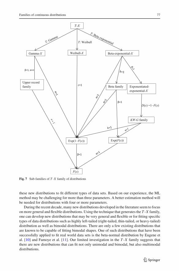
Figure 7 provides a tree-relationship of the T -X family addressed in this article. As Fig. 7shows, the T -X family consists of many sub-families, in which new distributions can bedefined and various existing distributions are special cases.

The variants of T -X families in Table 1 will define many potential new distributionsthat deserve further study. Some of these variants are currently under investigation. Futureresearch for the T -X family may include (i) the investigation of general properties of distribu-tions generated using different W (.) functions, (ii) defining and investigating the properties ofspecific new distributions, (iii) studying new methods for estimating the parameters in addi-tion to the well-known moments and maximum likelihood (ML) methods, and (iv) applying

123


Fig. 7 Sub-families of T -X family of distributions

these new distributions to fit different types of data sets. Based on our experience, the MLmethod may be challenging for more than three parameters. A better estimation method willbe needed for distributions with four or more parameters.

During the recent decade, many new distributions developed in the literature seem to focuson more general and flexible distributions. Using the technique that generates the T -X family,one can develop new distributions that may be very general and flexible or for fitting specifictypes of data distributions such as highly left-tailed (right-tailed, thin-tailed, or heavy-tailed)distribution as well as bimodal distributions. There are only a few existing distributions thatare known to be capable of fitting bimodal shapes. One of such distributions that have beensuccessfully applied to fit real world data sets is the beta-normal distribution by Eugene etal. [10] and Famoye et al. [11]. Our limited investigation in the T -X family suggests thatthere are new distributions that can fit not only unimodal and bimodal, but also multimodaldistributions.

123


This article focuses on the case when both T and X are continuous random variables.This technique can be extended to develop discrete T -X family of distributions where T iscontinuous and X is discrete. Different considerations for the W (.) functions will be needed.

Acknowledgements The authors are grateful for the comments and suggestions by the referees and theEditor-in-Chief. Their comments and suggestions have greatly improved the paper.

References

1. Akinsete, A., Famoye, F., Lee, C.: The beta-Pareto distribution. Statistics 42, 547–563 (2008)2. Alzaatreh, A., Famoye, F., Lee, C.: Gamma-Pareto distribution and its applications. J. Mod. Appl. Stat.

Methods 11(1), 78–94 (2012)3. Amoroso, L.: Ricerche intorno alla curva dei redditi. Annali de Mathematica 2, 123–159 (1925)4. Azzalini, A.: A class of distributions which includes the normal ones. Scand. J. Stat. 12, 171–178 (1985)5. Burr, I.W.: Cumulative frequency functions. Ann. Math. Stat. 13, 215–232 (1942)6. Cordeiro, G.M., de Castro, M.: A new family of generalized distributions. J. Stat. Comput. Simul. 81(7),

883–898 (2011)7. Cordeiro, G.M., Ortega, E.M.M., Nadarajah, S.: The Kumaraswamy Weibull distribution with application

to failure data. J. Frankl. Inst. 347, 1399–1429 (2010)8. Cordeiro, G.M., Pescim, R.R., Ortega, E.M.M.: The Kumaraswamy generalized half-normal distribution

for skewed positive data. J. Data Sci. 10, 195–224 (2012)9. de Castro, M.A.R., Ortega, E.M.M., Cordeiro, G.M.: The Kumaraswamy generalized gamma distribution

with application in survival analysis. Stat. Methodol. 8(5), 411–433 (2011)10. Eugene, N., Lee, C., Famoye, F.: The beta-normal distribution and its applications. Commun. Stat. Theory

Methods 31(4), 497–512 (2002)11. Famoye, F., Lee, C., Eugene, N.: Beta-normal distribution: bimodality properties and applications.

J. Mod. Appl. Stat. Methods 3(1), 85–103 (2004)12. Famoye, F., Lee, C., Olumolade, O.: The beta-Weibull distribution. J. Stat. Theory Appl. 4(2), 121–136

(2005)13. Ferreira, J.T.A.S., Steel, M.F.J.: A constructive representation of univariate skewed distributions. J. Am.

Stat. Assoc. 101(474), 823–829 (2006)14. Freimer, M., Kollia, G., Mudholkar, G.S., Lin, C.T.: A study of the generalized Tukey lambda family.

Commun. Stat. Theory Methods 17, 3547–3567 (1988)15. Fry, T.R.L.: Univariate and multivariate Burr distributions: a survey. Pak. J. Stat. Ser. A 9, 1–24 (1993)16. Galton, F.: Enquiries into Human Faculty and its Development. Macmillan & Company, London (1883)17. Gupta, R.D., Kundu, D.: Exponentiated-exponential family: an alternative to gamma and Weibull distri-

butions. Biom. J. 43, 117–130 (2001)18. Johnson, N.L.: Systems of frequency curves generated by methods of translation. Biometrika 36, 149–176

(1949)19. Johnson, N.L., Kotz, S., Balakrishnan, N.: Continuous Univariate Distributions, vol. 1, 2nd edn. Wiley,

New York (1994)20. Johnson, N.L., Kotz, S., Balakrishnan, N.: Continuous Univariate Distributions, vol. 2, 2nd edn. Wiley,

New York (1995)21. Jones, M.C.: Families of distributions arising from distributions of order statistics. Test 13(1), 1–43 (2004)22. Jones, M.C.: Kumaraswamys distribution: a beta-type distribution with tractability advantages. Stat.

Methodol. 6, 70–81 (2009)23. Karian, Z.A., Dudewicz, E.: Fitting Statistical Distributions—The Generalized Lambda Distribution and

Generalized Bootstrap Methods. Chapman & Hall/CRC Press, Boca Raton (2000)24. Kong, L., Lee, C., Sepanski, J.H.: On the properties of beta-gamma distribution. J. Mod. Appl. Stat.

Methods 6(1), 187–211 (2007)25. Kumaraswamy, P.: A generalized probability density functions for double-bounded random processes.

J. Hydrol. 46, 79–88 (1980)26. McDonald, J.B.: Some generalized functions for the size distribution of income. Econometrica 52,

647–663 (1984)27. Moors, J.J.: A quantile alternative for kurtosis. Statistician 37, 25–32 (1988)28. Mudholkar, G.S., Srivastava, D.K., Freimer, M.: The exponentiated Weibull family: a reanalysis of the

bus-motor-failure data. Technometrics 37(4), 436–445 (1995)

123


29. Nadarajah, S., Kotz, S.: The beta Gumbel distribution. Math. Probl. Eng. 4, 323–332 (2004)30. Nadarajah, S., Kotz, S.: The beta exponential distribution. Reliab. Eng. Syst. Saf. 91(6), 689–697 (2005)31. Pearson, K.: Contributions to the mathematical theory of evolution. II. Skew variation in homogeneous

material. Philos. Trans. Royal Soc. Lond. A 186, 343–414 (1895)32. Ramberg, J.S., Schmeiser, B.W.: An approximate method for generating symmetric random variables.

Commun. Assoc. Comput. Mach. 15, 987–990 (1972)33. Ramberg, J.S., Schmeiser, B.W.: An approximate method for generating asymmetric random variables.

Commun. Assoc. Comput. Mach. 17, 78–82 (1974)34. Ramberg, J.S., Tadikamalla, P.R., Dudewicz, E.J., Mykytka, E.F.: A probability distribution and its uses

in fitting data. Technometrics 21, 201–214 (1979)35. Shannon, C.E.: A mathematical theory of communication. Bell Syst. Tech. J. 27, 379–432 (1948)36. Song, K.-S.: Rényi information, log likelihood and an intrinsic distribution measure. J. Stat. Plan. Inference

93, 51–69 (2001)37. Tukey, J.W.: The practical relationship between the common transformations of percentages of counts and

amounts. Technical Report 36, Statistical Techniques Research Group, Princeton University, Princeton,NJ (1960)

123

A new method for generating families of continuous distributions

Documents

Transcript of A new method for generating families of continuous distributions