A New Measure of Horizontal Equity

Alan J. AuerbachUniversity of California, Berkeley and NBER

Kevin A. HassettAmerican Enterprise Institute

March 1999

We thank Nancy Nicosia for careful research assistance, Andy Mitrusi for his provision ofsimulations based on the NBER TAXSIM Model, and the Burch Center for Tax Policy andPublic Finance and AEI for research support. We also thank Jim Heckman, Louis Kaplow, JohnRoemer and participants in workshops at AEI, the Institute for Fiscal Studies, NYU Law School,and Georgetown Law Center for comments on earlier drafts.

Abstract

In this paper, we propose a new measure of horizontal equity that overcomes many of the

shortcomings of previous proposed measures. Our starting point is the observation that a well-

behaved social welfare function need not evaluate “global” (vertical equity) differences in after-

tax income using the same weights it applies to “local” (horizontal equity) differences, even

though this constraint has been applied in the past. Following work on the structure of individual

preferences, we show that a social welfare function can imply different preferences toward

horizontal and vertical equity. Adopting the general approach to the measurement of inequality

developed by Atkinson (1970), we use such a social welfare function to derive measures of

inequality that are decomposable into components naturally interpreted as indices of horizontal

and vertical equity. In particular, the former index measures deviations from the fundamental

principle that equals be treated equally.

Finally, we apply our new measure to two tax-return data sets, evaluating the degree to

which the horizontal equity of the US personal income tax has changed over time, and how

horizontal equity would be altered by one version of recent proposals to do away with the so-

called “marriage penalty.”

Alan J. Auerbach Kevin A. HassettDepartment of Economics AEIUniversity of California 1150 Seventeenth St. N.W.Berkeley, CA 94720-3880 Washington, DC 20036-4670auerbach@econ.berkeley.edu khassett@aei.org

JEL nos. D63, H22

“Nothing is so firmly believed as what we least know.”— Montaigne

I. Introduction

Among the normative foundations of modern tax systems, nothing is more contentious

than the question of how much the tax code should be utilized to redistribute income. Designers

of the tax code must assess potential reforms with an eye toward weighing the costs of foregone

redistribution against the efficiency benefits of flatter rate schedules, but there is little agreement

as to the appropriate weights to use. On the other hand, there is virtual unanimity that horizontal

equity – the extent to which equals are treated equally – is a worthy goal of any tax system.

Asked to choose between two otherwise identical tax systems that differed only in the extent to

which pre-tax equals faced different average tax rates, most would choose the system that had

the lowest “arbitrary” tax rate variation. While the measurement of vertical inequality, and the

impact of the tax code on it, is relatively straightforward, a workable definition of horizontal

equity has been elusive. From Musgrave (1959) on, there is general agreement that horizontal

equity is important, but little agreement on quite what it is.

Much work in the past few decades has focused on the constructing and refining

measures of horizontal equity. Rather than attempting to provide an exhaustive survey of this

work, we will simply highlight the key issues that have arisen and that are relevant to our own

work. First, there is the question of whether horizontal equity represents an independent concept

in the context of a general aversion to inequality. If society is generally averse to inequality in

the distribution of income, it has long been argued that horizontal equity will typically be implied

by this aversion. (See, e.g. the discussion in Atkinson 1980.) Thus, measures of horizontal

equity may simply represent components of overall measures of social welfare, and it is not clear

why they merit independent inspection or concern. Second, and related to this first point, if one

2

does impose independent criteria to assess horizontal equity that go beyond a general aversion to

inequality, it is necessary to justify these criteria, which are likely to stand in conflict with the

general aversion to inequality. The most common such additional criterion imposes an aversion

to changes in individuals’ relative standing in the income distribution, leading to measures of

horizontal equity based on rank reversals (e.g. Feldstein 1976, Rosen 1978, Plotnick 1981, King

1983). This approach has been criticized on the ground that it gives undue weight to the status

quo income distribution (Kaplow 1989).

Third, even if one does establish a case for an independent evaluation of horizontal

equity, it is necessary to define what is meant by “equals” and what we mean when requiring that

the tax system “treat equals equally.” Also, because deviations from equal treatment are

inevitable, we must specify how these deviations are to be evaluated. Even if one uses a simple

observable measure like pretax income to classify individuals, it remains unclear where to draw

the line in grouping individuals as equals. If our definition is not relevant for a comparison of

two individuals whose incomes differ by a penny, then it is of limited importance and one for

which a tiny change in income can induce large changes in measured horizontal equity.

In this paper, we develop a new measure of horizontal equity that derives from a general

aversion to inequality in the income distribution, without any appeal to additional criteria. Our

principal insight is that horizontal equity may represent a distinct and meaningful component of a

general evaluation of inequality, if “global” and “local” differences in tax burden are accorded

potentially different weights. We start with an analogy to individual preferences over

consumption at different dates and consumption at a given date over different states of nature.

While standard consumer preferences imply a link between aversion to differences in outcomes

across states of nature (risk aversion) and across time (imperfect intertemporal substitution),

3

various papers (e.g., Kreps and Porteus 1978, Epstein and Zin, 1989) have shown that this link

may be broken by relaxing the von Neumann-Morgenstern axioms of expected utility. We show

that an evaluation of the income distribution using a similar functional form can imply different

preferences toward horizontal equity and vertical equity, much as flexible individual preferences

have been used to distinguish between intertemporal substitution and risk aversion. Adopting the

general approach to the measurement of inequality developed by Atkinson (1970), we use such a

function to derive measures of inequality that are decomposable into components naturally

interpreted as indices of horizontal and vertical equity. In particular, the horizontal equity index

measures deviations from the fundamental principle that equals be treated equally. Finally, we

apply our new measure to two tax-return data sets, evaluating the degree to which the horizontal

equity of the US personal income tax has changed over time, and how horizontal equity would

be altered by one version of recent proposals to do away with the so-called “marriage penalty.”

II. The Model

As our focus here is on distributional issues, we ignore behavioral considerations and

assume that each individual’s income and tax payments are exogenous.1 There are a variety of

standard approaches to measuring inequality in the distribution of income, and measures of

horizontal and vertical equity in the literature that correspond to these alternatives approaches.

For example, one recent approach develops a measure of horizontal equity based on the Gini

coefficient of the post-tax income distribution (Aronson et al 1994), while another bases it

measure on mean logarithmic deviations in post-tax income (Lambert and Ramos 1997). Each

of these approaches imposes a specific metric for evaluating differences among individuals, and

1 More generally, one might use our approach using measures of individual welfare that took account of issues of taxincidence and deadweight loss.

4

it is unclear why one should prefer one to other or, for that matter, why still another might not be

preferred. Moreover, as Atkinson (1970) emphasized, measures that do not impose much

structure often are useful in a very restricted set of applications. Gini coefficients, for example,

are informative in the absence of a specification of social preferences only if the underlying

Lorenz curves do no cross. In his study of vertical equity, Atkinson demonstrated that a measure

based on a social welfare function with explicit preferences toward inequality could significantly

extend the reach of inequality inquiry. In the case of horizontal equity there are similar

problems, in particular, it is difficult to chose among the various methods without access to an

underlying objective function. Thus, rather than start with a metric, we start with a general

specification of preferences over individual after-tax incomes, with parameters that vary with the

degree of aversion to inequality that, in turn, imply a metric that is consistent with this

specification of preferences.

The concept of horizontal equity is based on the idea that there are classes of individuals

whom we would wish to label “equals.” Thus, let us begin with the simplifying assumption that

there are a finite number of income levels, say M, with Ni individuals at each level. More

generally, we might imagine these groups of equals as being defined by some characteristic, such

as family structure, age, or region of residence. Following Atkinson (1970), we start with a

flexible function based on individual after-tax incomes that imposes an aversion to inequality,

say γ, among different levels of after-tax income:

(1) ( ) γγ

−

= =

−

−= ∑∑

1

1

1 1

1M

i

N

jiji

i

Tyw

5

where yi is the before-tax income of individuals in group i, and Tij is the tax payment by the jth

individual in group i.

Expression (1) has two important properties. First, it respects the Pareto principle, in that

it is increasing in each person’s after-tax income. Second, it is increasing with respect to any

experiment that shifts income from an individual with higher after-tax income to one with lower

after-tax income. Thus, it simultaneously incorporates notions of vertical equity (a wish to

redistribute from the rich to the poor) and of horizontal equity (a wish to keep after-tax income

equal for those with the same before-tax income). Clearly, it requires some modification if it is

to give rise to an independent measure notion of horizontal equity.

The function in (1) constrains differences among individuals within any class i to induce

the same loss of social welfare as differences among individuals in different income classes. But

if horizontal equity is to have any independent content, it seems both necessary and appropriate

for attitudes to differ about these two types of inequality. Large differences among similar

individuals might be viewed as intrinsically arbitrary (regardless of whether or not they resulted

from intentionally “abusive” government behavior), and therefore more costly to the social

fabric; or they might simply be viewed as more costly because individuals compare themselves

to those with similar characteristics. This logic suggests that we replace (1) with

(2) ( )ρ

γρ

γ

−−−

=

−

=

−= ∑∑

1

1

1

1

1

1

1

1 iN

jiji

i

M

ii Ty

NNw

where ( now represents the inequality aversion within classes and D the inequality aversion

across classes. If ρ = γ, this reduces to expression (1). A similar functional form has been used

in the literature to distinguish between preferences with respect to consumption over time and, at

6

a given time, over states of nature. Just as we might wish to allow individuals to be more (or

less) averse to variations in consumption over states of nature than to variations in consumption

over time, we might wish to allow welfare to be more (or less) averse to the variations in after-

tax income within a certain group than to variations among individuals in different groups.2

Note that while the function in (2) still respects the Pareto principle, it does violate

another characteristic sometimes imposed on social welfare measures3, that a comparison of any

two outcomes should depend only on the well-being of individuals who are not indifferent to the

outcomes. For example, imagine that there are two income classes, two individuals in each

income class, and that γ > 0 and ρ = 0 (there is no aversion to inequality across classes). That is,

the function w may be written:

(3) ( ) ( )( ) ( ) ( )( ) γγγγγγ −−−−−− −+−+−+−= 1

11

2221

2121

11

1211

111 TyTyTyTyw

Further, assume for simplicity that y1 = y2 and that there are two outcomes, A and B, between

which the tax liabilities of individuals 12 and 22 do not change; let these fixed liabilities be 12T

and 22T , respectively. Suppose that under outcome A, T11 = x > 0 and T21 = 0, while under

outcome B, T21 = x and T11 = 0. Consider two possible situations. In one, 12T = x and 22T = 0; in

the other, 22T = x and 12T = 0. Then, in the first situation, A eliminates horizontal inequity and

will be preferred to B, while in the second case, B eliminates horizontal inequity and will be

preferred to A. That is, the relative weight given to individuals 11 and 21 will depend on the

2 Although we make the analogy here to household decisions under uncertainty, our own analysis focusesexclusively on the evaluation of ex post income distributions.3 See, for example, the discussion in Roemer (1996), chapter 4.

7

relative status of individuals 12 and 22. This dependence should not be surprising, for

comparisons across and within groups are presumed to differ in their relative importance.

Having provided scope for the independent evaluation of local differences, we must now

consider the issue of how to delineate groups of individuals, in this case income classes. One

might wish to posit that individuals belong to a small number of quite distinct groups of

“equals.” But whether our measure of similarity is income or an alternative like age or location,

the distribution much more closely resembles a continuum, with very small gaps between

contiguous groups and very few individuals with exactly the same characteristics. Thus, if we

define the preference parameter γ as applying only to individuals with precisely the same

income, it will have essentially no impact. Indeed, such a restriction seems inappropriate if our

intent is to define reference groups of “similar” individuals. But, if we define a group of equals

to include those with somewhat different incomes, the question remains how large that group

should be, and where to place its boundaries. It would seem that any group boundary would

impose an arbitrary discontinuity, with a small change in income inducing a large change in a

person’s membership in a particular reference group. Indeed, this discontinuity has been a

problem with past approaches based on discrete groupings of income classes. However, it is also

avoidable, because such unique income class definitions are unnecessary to compare each

individual to others with similar income.

As an alternative, we may define an appropriate reference group for each income level,

with such reference groups overlapping, rather than assigning each individual to only one income

class. We define these reference groups in terms of a density, or scaling, function, fi(⋅), that

applies at income level i, defined over group distance, as measured by the difference between yi

8

and the income of another group, say yk. With this, we generalize (2) so that γ applies within

reference groups4:

(4) ( )( )

( ) ( )γρ

γρ

−−

=

−

=

=

= =

−

−−⋅−

−= ∑∑

∑∑ ∑

1

1

1

1

1

1

1 1

1 1 kN

jkjk

M

kiki

k

M

kiki

M

ik

M

kiki Tyyyf

Nyyf

Nyyfw

When ρ = γ, this reduces to expression (1) if the scaling functions are defined so that

( ) 11

=−∑=

M

iiki yyf . Note that the summation here is over i, rather than k. That is, the sum of

weights applied to each household, not to each reference group, must sum to 1. To implement

this, we define the shape of fi(⋅) for each i, but let the sum ( ) i

M

kiki zyyf =−∑

=1

, where zi is

unknown, and then solve for the vector z so that ( ) .11

kyyfM

iiki ∀=−∑

=

In our applications below, we define income classes so that Nk is constant over k, and

assume that fi(⋅) is normally distributed, peaking at k = i. The smaller the standard deviation of

the normal distribution, the tighter the income range used to define a reference group for those in

income class i. Clearly, the shape of fi(⋅) is not predetermined. Like the inequality aversion

parameters ρ and γ, it depends on political and ethical considerations. However, the spirit of the

calculation would seem to rule out distributions that end abruptly, for these would be subject to

the critique leveled against other measures that small changes in income could lead to large

changes in measured horizontal equity.

4 We also take both sides of the equation to the power 1-ρ to make the expression less messy.

9

There is a certain analogy here between the specification of the function fi(⋅) to estimate

horizontal equity in the neighborhood of income level yi and the choice of a kernel in the

nonparametric estimation of the value of a function at a particular point in the function’s

domain. In that literature (e.g., Yatchew 1998), there is a trade-off between the extra information

gained from expanding the width of the kernel and the bias associated with using information

from observations that are increasingly dissimilar to the observation of interest. Here, we use

observations other than those exactly at yi because we believe they provide information about

conditions at yi. For example, if the tax system yields wildly different burdens for individuals

with incomes slightly different from yi, we believe that this tells us something about horizontal

equity at yi, where there may be very few observations with exactly that level of income. On the

other hand, as the distance from yi grows, the similarity of individuals to those at yi falls. The

“correct” kernel width should depend on how much noise we believe there is in yi as an indicator

of “true” income class.

For compactness of notation, we express fi(⋅) below as a function of the index gap, k-i,

rather than the income difference yk-yi. We also suppress the limits of summation, which are the

same as those in expression (4). We can rewrite (4) as:

(5) ( ) ( ) ( ) ( ) ( )( )

γρ

γρρρ

−−

−−−−

−

−−⋅

−−

−= ∑∑∑∑ ∑

1

1

1111

~1~11~1~

j ii

kjk

ki

kkii

iik

ki ty

tyikf

NikftyNikfw

where ~yi and ~ti are (as yet undefined) “representative” values for class i and t T ykj kj k= / is the

average tax rate for the jth member of group i. We wish to define ~yi and ~ti in a way that makes

the last term measure horizontal equity. Rewrite (5) as:

10

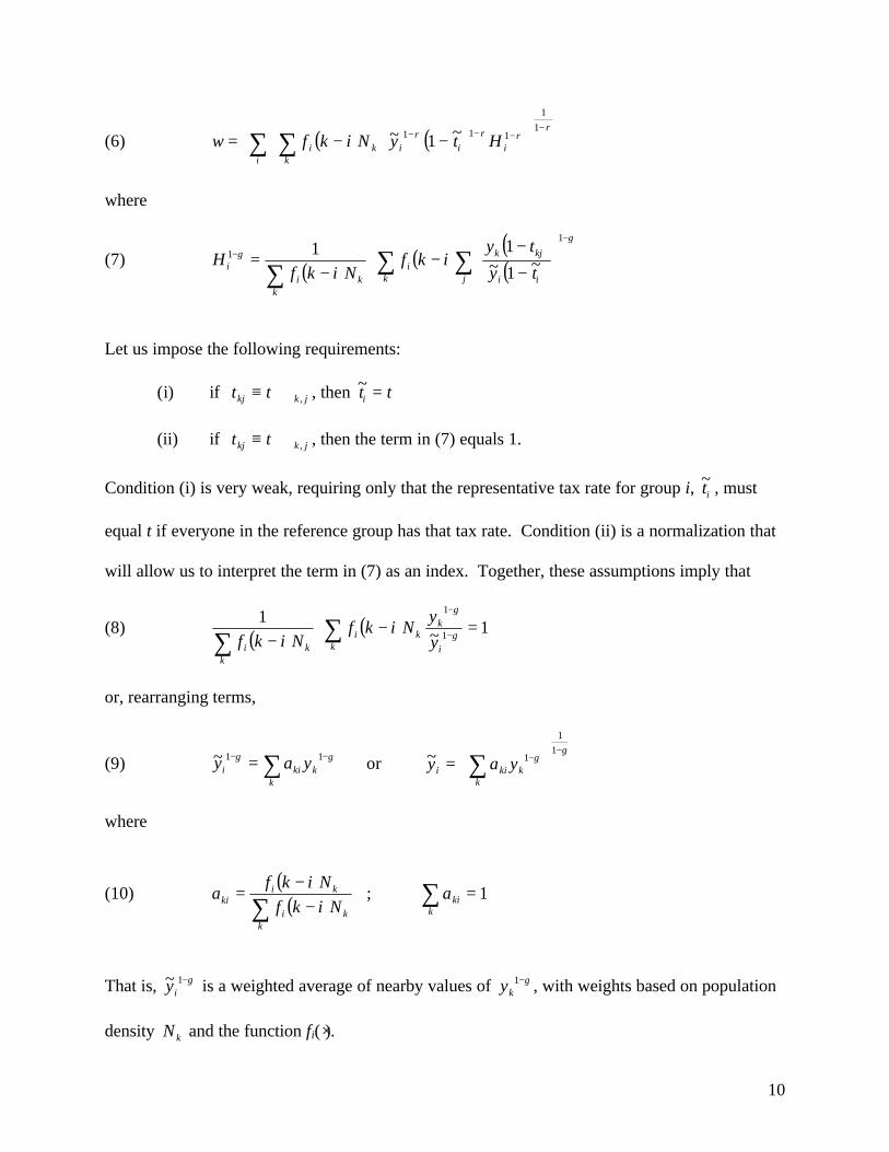
(6) ( ) ( )ρ

ρρρ−

−−−

−

−= ∑ ∑

1

1

111 ~1~i

iii

kki HtyNikfw

where

(7) ( ) ( ) ( )( )

γ

γ

−

− ∑∑∑

−

−−⋅

−=

1

1~1~

11

j ii

kjk

ki

kki

i ty

tyikf

NikfH

Let us impose the following requirements:

(i) if t tkj ≡ ∀k j, , then ~t ti =

(ii) if t tkj ≡ ∀k j, , then the term in (7) equals 1.

Condition (i) is very weak, requiring only that the representative tax rate for group i, ~ti , must

equal t if everyone in the reference group has that tax rate. Condition (ii) is a normalization that

will allow us to interpret the term in (7) as an index. Together, these assumptions imply that

(8) ( ) ( ) 1~1

1

1

=−⋅− −

−

∑∑ γ

γ

i

k

kki

kki y

yNikf

Nikf

or, rearranging terms,

(9) γγ −− ∑= 11~k

kkii yay or ~y a yi ki k

k

=

−

−

∑ 1

1

1γ

γ

where

(10)( )

( )∑ −−

=

kki

kiki Nikf

Nikfa ; aki

k

=∑ 1

That is, ~yi1−γ is a weighted average of nearby values of yk

1−γ , with weights based on population

density N k and the function fi(⋅).

11

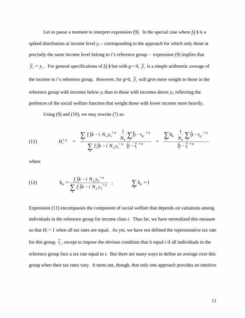
Let us pause a moment to interpret expression (9). In the special case where fi(⋅) is a

spiked distribution at income level yi – corresponding to the approach for which only those at

precisely the same income level belong to i’s reference group – expression (9) implies that

ii yy =~ . For general specifications of fi(⋅) but with γ = 0, iy~ is a simple arithmetic average of

the income in i’s reference group. However, for γ>0, iy~ will give more weight to those in the

reference group with incomes below yi than to those with incomes above yi, reflecting the

prefences of the social welfare function that weight those with lower income more heavily.

Using (9) and (10), we may rewrite (7) as:

(11)

( ) ( )( ) ( )

( )( ) γ

γ

γγ

γγ

γ−

−

−−

−−

−

−

−⋅=

−⋅−

−⋅−=

∑ ∑

∑

∑ ∑1

1

11

11

1

~1

11

~1

11

i

k jkj

kki

kikki

k jkj

kkki

it

tN

b

tyNikf

tN

yNikf

H

where

(12) ( )

( )∑ −

−

−

−=

kkki

kkiki

yNikf

yNikfb

γ

γ

1

1

; bkik

=∑ 1

Expression (11) encompasses the component of social welfare that depends on variations among

individuals in the reference group for income class i. Thus far, we have normalized this measure

so that Hi = 1 when all tax rates are equal. As yet, we have not defined the representative tax rate

for this group, ~ti , except to impose the obvious condition that it equal t if all individuals in the

reference group face a tax rate equal to t. But there are many ways to define an average over this

group when their tax rates vary. It turns out, though, that only one approach provides an intuitive

12

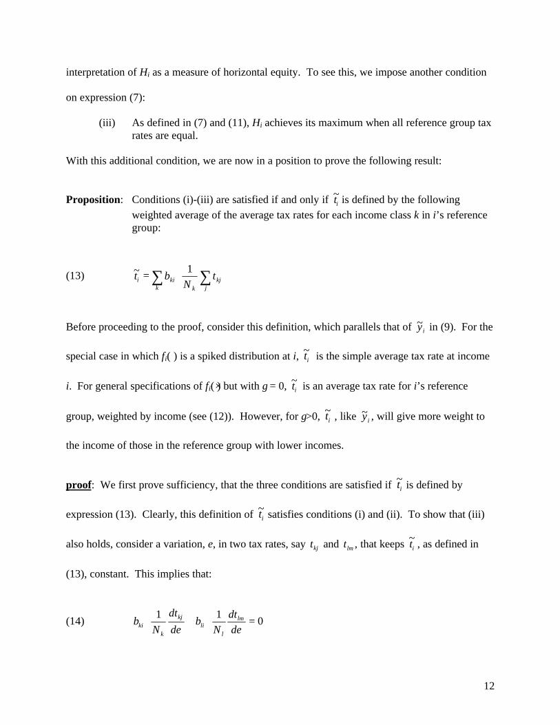
interpretation of Hi as a measure of horizontal equity. To see this, we impose another condition

on expression (7):

(iii) As defined in (7) and (11), Hi achieves its maximum when all reference group taxrates are equal.

With this additional condition, we are now in a position to prove the following result:

Proposition: Conditions (i)-(iii) are satisfied if and only if it~ is defined by the following

weighted average of the average tax rates for each income class k in i’s referencegroup:

(13) ∑ ∑

=

k jkj

kkii t

Nbt

1~

Before proceeding to the proof, consider this definition, which parallels that of iy~ in (9). For the

special case in which fi(⋅) is a spiked distribution at i, it~ is the simple average tax rate at income

i. For general specifications of fi(⋅) but with γ = 0, it~ is an average tax rate for i’s reference

group, weighted by income (see (12)). However, for γ>0, it~ , like iy~ , will give more weight to

the income of those in the reference group with lower incomes.

proof: We first prove sufficiency, that the three conditions are satisfied if it~ is defined by

expression (13). Clearly, this definition of it~ satisfies conditions (i) and (ii). To show that (iii)

also holds, consider a variation, ε, in two tax rates, say tkj and tlm , that keeps ~ti , as defined in

(13), constant. This implies that:

(14) 011

=⋅+⋅εε d

dt

Nb

d

dt

Nb lm

lli

kj

kki

13

The derivative of γ−1iH with respect to this same variation is proportional to5:

(15) ( ) ( ) ( ) ( )ε

γε

γ γγ

d

dtt

Nb

d

dtt

Nb lm

lml

likj

kjk

ki−− −⋅−−−⋅−− 1

111

11

Substituting (15) into (14) yields:

(16) ( ) ( ) ( )[ ]γγ

εγ −− −−−⋅−− lmkj

kj

kki tt

d

dt

Nb 11

11

which vanishes when t tkj lm= . This will hold for all variations in tax rates if and only if ttkj ≡

∀k j, , for some value t. Although this result concerns εγ ddH i−1 , it also holds for

(17) ( )εγε

γ

γγ

d

dHH

d

dH ii−

−−−

−=

11

1

11

1

1,

which will not vanish unless εγ ddH i−1 does.

When t tkj lm= , the second-order condition for γ−1iH with respect to ε based on (16) (again

using (14) to substitute into the expression) is:

(18) ( ) ( ) ( )

−+

−

−−

+−+−

lli

lm

kki

kjkj

k

ki

Nb

t

Nb

t

d

dt

N

b )1()1(211

1γγ

εγγ ,

which has the same sign as -(1-γ). Given the relationship between γ−1iH and Hi, this implies that

the second-order conditions for a maximum for Hi are satisfied when all tax rates are equal.

5 The denominator in (11) is fixed by assumption; the term in (15) is the change in the numerator in (11).

14

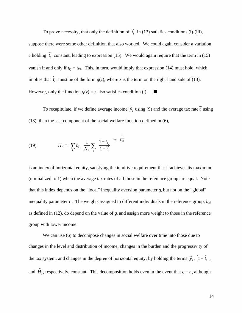
To prove necessity, that only the definition of it~ in (13) satisfies conditions (i)-(iii),

suppose there were some other definition that also worked. We could again consider a variation

ε holding it~ constant, leading to expression (15). We would again require that the term in (15)

vanish if and only if tkj = tlm. This, in turn, would imply that expression (14) must hold, which

implies that it~ must be of the form g(z), where z is the term on the right-hand side of (13).

However, only the function g(z) = z also satisfies condition (i). �

To recapitulate, if we define average income ~yi using (9) and the average tax rate ~ti using

(13), then the last component of the social welfare function defined in (6),

(19) H bN

t

ti kik k

kj

ij

= ⋅−−

∑ ∑− −1 1

1

11

1

~

γ γ

is an index of horizontal equity, satisfying the intuitive requirement that it achieves its maximum

(normalized to 1) when the average tax rates of all those in the reference group are equal. Note

that this index depends on the “local” inequality aversion parameter γ, but not on the “global”

inequality parameter ρ. The weights assigned to different individuals in the reference group, bki

as defined in (12), do depend on the value of γ, and assign more weight to those in the reference

group with lower income.

We can use (6) to decompose changes in social welfare over time into those due to

changes in the level and distribution of income, changes in the burden and the progressivity of

the tax system, and changes in the degree of horizontal equity, by holding the terms ~yi , ( )1 − ~ti ,

and ~H i , respectively, constant. This decomposition holds even in the event that γ = ρ, although

15

the motivation for the exercise, notably the specification of a reference group through the

definition of f(⋅), clearly hinges on the fact that this equality need not hold.

An issue that has often arisen in the literature is how we should weight local measures of

horizontal equity into a single, overall index. For measures that start with some assumed metric

for measuring deviations, there may be no obvious answer. Here, though, because our metric is

defined by an underlying welfare function, the answer is dictated by decomposition procedure

just followed. We may define an aggregate index of horizontal equity as that constant value, H~

,

for which the social welfare function takes on the same value as it does for the given values of

Hi:

(20)

( ) ( )

( ) ( )

ρ

ρρ

ρρρ−

−−

−−−

−

−

−

−=

∑ ∑

∑ ∑1

1

11

111

~1~

~1~~

iii

kki

ii

iik

ki

tyNikf

HtyNikf

H

This overall index does depend on D. Intuitively, we will care more about horizontal equity at

lower income levels, the larger is the value of ρ, because we care more, in general, about what

happens to lower-income individuals.

III. Discussion

Before presenting empirical applications of the measure just derived, it will be useful to

review some of its attributes, in light of the difficulties mentioned above in the introduction.

First of all, the measure is derived from a well-behaved social welfare function, so it will

not lead to any anomalies inherent in alternative approaches that do not, for example, respect the

Pareto principle in a world of certainty. While we claim no particular knowledge of the

function’s specific parameter values, the approach provides a framework with logical

16

foundations that can serve as a useful tool for evaluating alternative policy options. It allows

those performing the evaluation to specify their own preferred parameter values within a single

framework, rather than having the values be implicit in the choice of one measure over another.

As discussed above, the particular functional form used here does allow the well-being of

reference group members to be relevant to comparisons of alternative outcomes, even if these

members themselves are indifferent between such outcomes. Also, because the function is

concave in the assumed linear individual utilities, its use in evaluating uncertain outcomes would

not satisfy the Pareto criterion as characterized in terms of individual, ex ante, expected utilities.6

We view neither of these attributes as particularly problematic. As discussed above, the whole

notion of horizontal equity suggests the relevance of reference groups; that such groups should

matter should hardly be seen as an anomaly. The extension of the Pareto principle to apply to ex

ante expected utilities requires not only that individual preferences satisfy the von Neumann-

Morgenstern axioms, but also that social welfare cannot be averse to ex post inequalities in the

distribution of income, a requirement that strikes us as unnecessarily restrictive. How to think

about equity in general and horizontal equity in particular becomes more complicated in the

presence of uncertainty, and is not a subject pursued further here.

Second, the measure is scaled in the same units as other factors that determine social

welfare, so we can make meaningful comparisons between a change in horizontal equity and,

say, an increase in overall taxes or a decrease in the dispersion of income. Third, because the

measure of horizontal equity is derived through a decomposition of the social welfare function

(see (6)), there is no problem in potential “double-counting” of variations that affect both

horizontal and vertical equity. A change in any individual’s tax burden will affect the social

6 For example, since utility is linear in income, individuals would be willing to take on any risk in exchange for anarbitrarily small compensation, whereas society would not if it maximizes expected social welfare.

17

welfare function through many channels, some through different indices Hi and some through

average tax rates it~ , but these effects will each be distinctly measured. Finally, the measure

allows great flexibility in the definition of “equals,” so that small variations in income need not

trigger discontinuous changes in reference group membership.

This new measure also suggests a response to a problem raised in the literature by Stiglitz

(1982), who observed that, in a more complicated model of the economy, the “utility possibilities

frontier” facing the social welfare planner might not be convex.7 In such a situation, as depicted

by Atkinson (1980) and repeated in Figure 1, the government might improve social welfare by

providing two otherwise identical individuals with different tax burdens and utility levels, as

depicted at points A and B. Based on this result, one can argue that horizontal equity need not be

subsumed by general social welfare maximization, and that, if horizontal equity is desirable in its

own right, it might be appropriately included as a separate argument of the social welfare

function. In a sense, this is precisely what our approach does. By allowing social welfare to be

more averse to horizontal inequity than to vertical inequity, it can permit outcomes that push

“equals” closer together. Indeed, for sufficiently HE-averse preferences – the extreme being the

Leontief preferences depicted by the dashed social indifference curve in Figure 1 – no horizontal

inequity would result, for then point C would be most preferred. However, our approach has the

advantage that this outcome is generated in the context of social welfare maximization, and does

not require the inclusion of an ad hoc, distinct measure of horizontal equity subject to the various

problems touched on above.

Figures 2 and 3 illustrate the ability of our social welfare function to accommodate

sharply different preferences toward horizontal and vertical inequality. They illustrate a simple

7 With income and taxes exogenous in our model, the frontier is linear.

18

economy with three individuals. Mr. 1 is poor, having roughly half the income of Mr. 2 and Mr.

3, who are a single comparison class for the purposes of horizontal equity. The origin, which is

the set of incomes {0.2, 2, 2}, is in the back left hand corner. In the first example, Figure 2, ρ =

γ =2, so the aversion to horizontal inequality is not particularly strong.8 Since Mr. 1 is poorer

than the others, we need to give Mr. 2 and Mr. 3 much more income than we take away from Mr.

1 in order to maintain indifference. But the indifference surface is relatively flat in the Mr.2-Mr.

3 plane: inequality between Mr. 2 and Mr. 3 is not heavily penalized. Figure 3 increases the

parameter γ to 50, making preferences toward horizontal inequality between Mr. 2 and Mr. 3

almost Leontief. As income is taken away from Mr. 1, the total income that must be devoted to

Mr. 2 and Mr. 3 to maintain indifference is much lower when they receive the same income.

IV. Initial Applications

To illustrate our measure of horizontal equity, we use two data sets. Each is a public-use

sample of individual income tax returns. The first, the Michigan tax panel, has the advantage of

following the same group of taxpayers over time, but also has two disadvantages. It has a

relatively small number of households (about 5,000) and a terminal year of 1990, before many of

the recent changes in the income tax code took place. Our second data set, the annual NBER tax

file, does not provide the advantages of a panel, but has several other advantages. First, it is

currently available for 1994 – after the 1993 tax increase. Moreover, it has roughly 96,000

households, with the added benefit of significant oversampling of high-income households.

Finally, in conjunction with the NBER TAXSIM model, this data set can be used to simulate the

effects of a tax law change on household tax liabilities.

8 For simplicity, we are assuming here that the function f(⋅) is a spike, so that Mr. 1 is not in the reference group forMr. 2 and Mr. 3, and vice-versa.

19

We examine first the results from the Michigan panel. For this data set, we define each

household to be its own income class. That is, we set Ni = 1 ∀i. Initially, we consider each

household without regard to its filing status or the number of individuals in the household. That

is, for each household, we consider only adjusted gross income (AGI) and federal income tax.

Figure 4 presents graphs of Hi for the panel, with both income and tax liability averaged

over the panel’s 12-year period. Our sample of 5022 consists of all observations with complete

income and tax data for the full period, less 216 households that appeared to have anomalous tax

or income patterns, based on very gross filters.9 For this and most other figures that follow, we

plot Hi against household income percentile. To calculate a household’s percentile in the income

distribution, we first order households in ascending order of average income, giving each

household its 12-year average sample weight, and then dividing by the sum of average sample

weights. Thus, the household with income greater than other households with 35 percent of the

sample weight will be located at the 35th percentile of the income distribution. Because the

values of Hi trend downward at the very top of the distribution, we truncate the graphs at the 98th

percentile in order to make more subtle variations at other incomes distinguishable.

The figure presents nine different graphs of Hi, based on all possible combinations of

three different assumptions about the “local” inequality aversion parameter, γ, and three different

shapes of the function fi(⋅). For γ, we consider values of .5, 2, and 5, meant to reflect very wide

variation in preferences, from mild to strong aversion to inequality. For fi(⋅), we use the normal

distribution, letting this distribution vary with respect to the degree of reference group dispersion

– the distribution’s standard deviation – and the extent to which this dispersion changes with

9 Most of the households eliminated had negative AGI or a tax rate greater than 100 percent in at least one panelyear. A small additional number were eliminated because of a tax rate that deviated by more than 25 percentagepoints from the household’s 12-year average in any year. We omitted one additional household with a hugedeviation in income to near 0 in one year.

20

income.10 We consider three patterns. One specification sets the standard deviation equal to

.10yi. The second specification, which we refer to as “log” scaling, sets the standard deviation

equal to x ln(yi), with x scaled so that the distribution is the same at median income, ym, i.e., x =

.10ym/ln(ym). These two specifications of fi(⋅) differ in the extent two which the relevant

“distance” for membership in an income level’s reference group grows with income. The first

approach assumes that the distance grows in proportion to income, so that an individual with an

income of $100,000 would be as relevant for reference when yi = $200,000 as an individual with

an income of $10,000 would be for yi = $20,000. The log scaling approach slows this widening

of the income dispersion of the reference group, implying that the relative weight given to

someone with $10,000 of income in the second case would correspond to the weight given to

someone with $182,000 of income in the first case, rather than $100,000. Our third specification

for fi(⋅) also uses log scaling, but with a larger value of x, .25 rather than .10.

Figure 4 provides a number of interesting results. First, our measure of horizontal equity

generally falls with γ – the greater the aversion to local inequality, the lower the index of

horizontal equity. This is hardly surprising – we would expect to be willing to “pay more” to

avoid dispersion, the higher our aversion to it. We can scale the values of Hi in terms of an

equivalent increase in the average tax rate, it~ . From (6), the increase in the tax rate, say ∆i, that

has the same impact on social welfare as the deviation of Hi from 1, is:

(21) ∆i )~1)(1( ii tH −−=

Thus, for values of Hi near .9950-.9975, the range for γ = 5, and it~ around .15, ∆i equals roughly

.002 to .004, or .2 to .4 percentage points. That is, the existing horizontal equity, as measured,

10 Because the income distribution is bounded, the distributions actually used are truncated normals.

21

costs society as much as an across-the-board increase of .2 to .4 percentage points in the average

income tax rate.

One might be interested in how Hi varies with income rather than location in the income

distribution. Figure 5 repeats one of the nine graphs of Hi from Figure 4, for γ = 2 and log

scaling of .10, against two alternative series on the horizontal axis: income percentile (bottom

axis), as in Figure 4, and real (1990$) income (top axis). Because of the skewness of the income

distribution, the second curve is compressed to the left, relative to the first.

A central question that always arises in attempting to define horizontal equity – and one

which our new approach must confront as well – is which adjustments are “correct” – moving

the tax burden closer to equitable – and which adjustments represent deviations from an

equitable outcome. One could always do away with any measured horizontal inequity simply by

assuming that any differences in burden between apparent equals are due to the fact that they

really do differ in some respect that is being recognized by the tax system.

For example, if a certain expense, say for medical care, should not be counted as income,

then allowing a deduction for it should improve our measure of horizontal equity, if we also

measure income by subtracting this expense. On the other hand, if we ignore such “appropriate”

adjustments to income in our computation, then we may see a deviation in an average tax rate

where none really exists. Thus, the accuracy of our measure of horizontal equity depends on

whether we have made the right adjustments to income. We do not wish to pursue this issue

fully here, but one important potential adjustment that relates to our consideration of the

marriage penalty relates to household size, in particular the number of adults in a household.

Presumably, the view that such an adjustment is needed underlies the fact that married

couples who file jointly receive a larger standard deduction and wider tax brackets than single

22

filers. Indeed, the notion of a “marriage tax” seems predicated on the view that the tax system

doesn’t adjust enough for joint filers. But this leaves the question of how much we should adjust

the income level of a joint-filing household in order to compare it to that of a single filer. Figure

6 considers three alternatives.11 For the reference group function, fi(⋅), based on the .10 log

scaling assumption, and all three values of γ from Figure 1, we measure each household’s

income (and taxes) at its original value, its original value divided by 2 , and its original value

divided by 2. That is, we consider equivalence scales of 1, 2 , and 2, in deciding how to

describe the taxes and income per “unit” in the household. The logic of not dividing by 2 is that

there are economies of scale in living arrangements, so that the living standard for joint filers

may be higher than that of single filers with half their combined income.12

A striking pattern in the figure is that as the adjustments by 2 and then 2 are made in

succession, the Hi curves rise almost uniformly. This result suggests that horizontal inequity

may not be as bad as the unadjusted curves suggest. But it also has another interpretation, if we

think that the full adjustment by 2 represents an excessive correction: that one of the sources of

horizontal inequity may be the overcorrection of tax brackets for joint filers. We return to this

issue below, when considering the impact of potential reforms.

Figure 7 presents Hi curves for each individual year in the Michigan tax panel, using the

full sample of 5,022, for .10 log scaling and γ = 2. The evolution of the curves is quite

interesting, in light of the fact that the two most important tax changes occurred in 1981, with the

passage of the Economic Recovery Tax Act, and in 1986, with the Tax Reform Act of 1986. The

11 For this figure, we eliminated all observations that experienced a change in filing status during the 12-year period,moving us from a sample of 5,022 to one of 3,389.12 Below, when discussing the marriage penalty, we consider additional adjustments for family size. Determiningthe adjustment most appropriate for evaluating tax payments is a subject worthy of further discussion, but beyondthe scope of our current analysis.

23

most striking pattern in the figure is the general shift upward over time, at least since 1981,

which is for most of the income distribution the lowest curve in the figure. Indeed, for most

income levels above the 25th percentile, the curves for years 1987-1990 – the only four years in

the sample after the individual income tax provisions of the 1986 act took effect – are the four

highest in the figure. Only at lower income levels is the pattern different. There, the years 1979

and 1980 rate highest. From this simple analysis, one might tentatively conclude that the 1981

act worsened horizontal equity at most income levels, particularly at the low end, and that the

1986 act reversed the pattern, particularly at middle and upper income levels.

V. The Marriage Penalty

In Figure 8, we turn to our second data set, the NBER 1994 sample. Because of the size

of this data set – 90,13213 – it was computationally infeasible to define each individual

observation as an income group. Instead, we defined each group i to include 20 individuals,

producing a similar number of groups – 4,506 – as in the previous exercise.14 Figure 8 repeats

the graphs of Hi, for .10 log scaling, γ = .5 and 2, and joint filer adjustments of 1, 2 , and 2.

The general patterns are similar to those observed earlier, particularly that for 1990 in Figure 7,

with a general downward drift in Hi as income rises, followed by a slight rise around the 70th

percentile, and then a resumption of the downward trend, accelerating near the top. One

interesting difference is that the impact of the size adjustment to income for joint filers appears to

raise Hi less than was the case for the 1979-90 average. Taking a “reverse engineering”

approach and asking what “correct” joint filer size adjustment would be “implied by” the 1994

13 This number is net of the elimination of 6,252 records with negative AGI or a tax rate over 100 percent.14 For simplicity, to make the number of observations divisible by 20, we randomly dropped 12 observations.

24

tax system if that system’s tax adjustments were designed to minimize horizontal equity, would

imply a smaller such adjustment than would the earlier tax system.

How would these results differ if we attempted to “solve” the marriage penalty? As is

well known, finding such a solution presents a problem much thornier than is sometimes

suggested in political debates. Even comparing joint filers to two single filers in identical

circumstances, the effect of marriage is often to reduce taxes rather than to raise them, leading

not to a marriage penalty but a marriage “bonus.” (CBO 1997). Even more problematic is the

question of how to compare joint filers with individual single filers in different situations – the

question posed above when considering the “appropriate” joint filer adjustment for measuring a

family’s income level. Still, many alternative “solutions” to the marriage penalty have been

proposed, generally structured to reduce the taxes of joint filers. We consider the impact of one

such scheme, which would divide all income of joint filers equally between spouses, along with

deductions and exemptions not directly tied to either taxpayer, and then allowing each spouse to

file as a single taxpayer. This scheme is roughly equivalent to providing joint filers with tax

brackets that are twice as large as those facing single filers. Clearly, such a scheme would

reduce the taxes of nearly all joint filers, because the current brackets are based on a lower

ratio.15 But whether this improves horizontal equity or not depends on whether joint filers now

face burdens higher than those of single filers to whom they are being compared. The relevant

comparison groups, in turn, depend on how we adjust for family size when computing income.

15 The zero-bracket amount for a joint-filing couple, equal to the standard deduction plus two exemptions, is $11,650for 1998, or roughly 1 2/3 times the single filer’s zero-bracket amount of $6,950. The next two bracket floors, forthe 28% and 31% rates, roughly preserve this ratio, at $42,350 and $102,300 for joint filers and $25,350 and$61,400 for single filers. However, the floors for the last two brackets (36% and 39.6%) for joint filers are 1.2 and1.0 times those of single filers.

25

Figures 9-11 illustrate the effect of this change on our measure of horizontal equity. Each

figure repeats two of the six graphs from Figure 8, for γ = .5 and 2 and one of the three joint filer

size adjustments, and also presents two comparable graphs for the alternative tax system aimed

at “solving” the marriage penalty. Figure 9 makes no joint filer adjustment, Figure 10 divides

the income of joint filers by 2 , and Figure 11 divides income of joint filers by 2.

Not surprisingly, the results in Figure 9 suggest that horizontal equity falls. If no family

size adjustment were appropriate, then the current tax system already would be too generous to

joint filers, and this system would exacerbate this bias. The pattern of this impact, occurring

primarily in the upper-middle income range, may be attributable in part to the fact that the

current tax system becomes less favorable to joint filers as incomes rise (see footnote 15). Thus,

if we view size adjustments as inappropriate, we are closer to the correct treatment under current

law and deviate more from this treatment under the proposal. However, this intuition fails to

explain why there is no apparent worsening of horizontal equity at lower income levels.

Figure 10 illustrates the impact of reform if the appropriate income adjustment is to

divide joint income by 2 . The pattern is similar to that in Figure 9. As expected, the decline

in measured horizontal equity is smaller in general, because the appropriate treatment is now

assumed to involve some family size adjustment. Again, though, the pattern observed for

incomes below the median, in this case showing a small improvement in horizontal equity, is

difficult to reconcile with the fact that the tax system is moving farther away from the size

adjustment assumed to be appropriate.

The adjustments in Figure 11 are based on an equivalence scale of 2, essentially

consistent with the policy being undertaken. If the only systematic variation in tax burdens

between single filers and joint filers under current law were attributable to differences in tax

26

schedules, the new tax policy would eliminate all horizontal equity attributable to differences in

filing status. Yet measured horizontal equity does not rise uniformly in the figure. Rather, it

rises at lower income levels, as before, and now also at higher income levels, but still falls at

middle income levels. This confirms what the other figures suggest, that the relative treatment of

joint filers and single filers under the current code differs in ways not captured by the tax

schedule itself, with these differences varying over the income distribution.

One systematic difference clearly omitted thus far is the presence of dependents, for

whom the tax code provides additional exemptions. This likely reduces the relative tax burdens

of joint filers, and might help explain why the reform appears to worsen horizontal equity at

some income levels, even in Figure 11. But ignoring dependents also means that we are

probably adjusting family size incorrectly, and therefore understating the extent to which joint

filers, who are more likely to have dependents, are unfavorably treated under current law.

Figures 12 and 13 illustrate the impact of the tax reform, now adjusting family income by

N and N, respectively, where N is the total number of individuals in the family’s household.

As one might expect, the latter figure now shows that the proposed reform raises horizontal

equity at all income levels, for it is based on a size adjustment that implies that the current tax

system treats joint filers with dependents far too severely. But adjusting by N still leaves a

large share of the income distribution over which the index falls. This suggests that joint filers

may be taking greater advantage of other provisions in the tax code that reduce tax payments (for

example, mortgage interest deductions), making their current treatment more favorable than is

implied by the simple rate schedules themselves.

Together, these figures confirm that the extent to which the marriage penalty should be

“corrected” depends on how great it is measured to be at present. But they also suggest that,

27

whatever the proper adjustment for the income of joint filers, the penalty may be least in need of

correction at upper middle income levels.

VI. Conclusions

We have derived a measure of horizontal equity that allows for separate social

preferences toward vertical and horizontal equity. As an illustration of the application of our

measure, we have explored the change in horizontal inequality of the U.S. federal income tax,

and examined a recent proposal to undo the “marriage penalty”.

Conditional on known values of preferences toward vertical and horizontal inequality,

our work is a contribution to the positive theory of measurement. While we are unaware of any

fundamental normative justification for the constraint – which has so often been imposed in the

past – that society’s preferences toward the two types of inequality by identical, there is also

little guidance as to the appropriate relative weighting, or how to determine individual reference

groups. The exploration of the consequences of different attitudes toward horizontal and vertical

inequality is an important subject of future inquiry.

28

References

Aronson, J. Richard, Paul Johnson, and Peter J. Lambert, 1994, “Redistributive Effect andUnequal Income Tax Treatment,” Economic Journal 104, March, 262-70.

Atkinson, Anthony B., 1970, “On the Measurement of Inequality,” Journal of Economic Theory2, 244-63.

Atkinson, Anthony B., 1980, “Horizontal Equity and the Distribution of the Tax Burden,” in H.Aaron and M. Boskin, eds., The Economics of Taxation, Brookings Institution,Washington, 3-18.

Congressional Budget Office, 1997, For Better or for Worse: Marriage and the Federal IncomeTax, June, 1-56.

Epstein, Larry G. and Stanley E. Zin, 1989, “Substitution, Risk Aversion, and the TemporalBehavior of Consumption and Asset Returns: A Theoretical Framework, Econometrica57, July, 937-69.

Feldstein, Martin, 1976, “On the Theory of Tax Reform,” Journal of Public Economics 6,July/August, 77-104.

Kaplow, Louis, 1989, “Horizontal Equity: Measures in Search of a Principle,” National TaxJournal 42, 139-54.

Kreps, David, and Evan L. Porteus, 1978, “Temporal Resolution of Uncertainty and DynamicChoice Theory,” Econometrica 46, January, 185-200.

King, Mervyn, 1983, “An Index of Inequality: With Applications to Horizontal Equity andSocial Mobility,” Econometrica 51, January, 99-115.

Lambert, Peter J. and Xavier Ramos, 1997, “Horizontal Inequity and Vertical Redistribution,”International Tax and Public Finance 4, January, 25-37.

Musgrave, Richard A., 1959, The Theory of Public Finance, McGraw-Hill, New York.

Plotnick, Robert, 1981, “A Measure of Horizontal Inequity,” Review of Economics and Statistics63, May, 283-88.

Roemer, John E., 1996, Theories of Distributive Justice, Harvard University Press, Cambridge.

Rosen, Harvey S., 1978, “An Approach to the Study of Income, Utility, and Horizontal Equity,”Quarterly Journal of Economics 92, May, 307-22.

29

Stiglitz, Joseph E., 1982, “Utilitarianism and Horizontal Equity: The Case of Random Taxation,”Journal of Public Economics 18, 1-33.

Yatchew, Adonis, 1998, “Nonparametric Regression Techniques in Economics,” Journal ofEconomic Literature 36, June, 669-721.

Figure 1. Horizontal Equity and Nonconvexity

high γlow γ

A

B

C

U1

U2

Figure 2. Social Welfare Function Indifference Surface(γ=2, ρ=2)

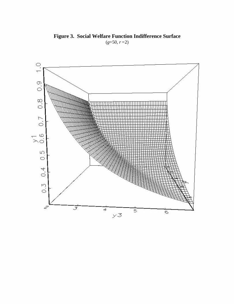
Figure 3. Social Welfare Function Indifference Surface(γ=50, ρ=2)

Figure 4. Index of Horizontal Equity: 12-Year Average, 1979-90(γ = .5,2, 5; Scaling = .10, Log Scaling = .10, .25)

Income Percentile

Index

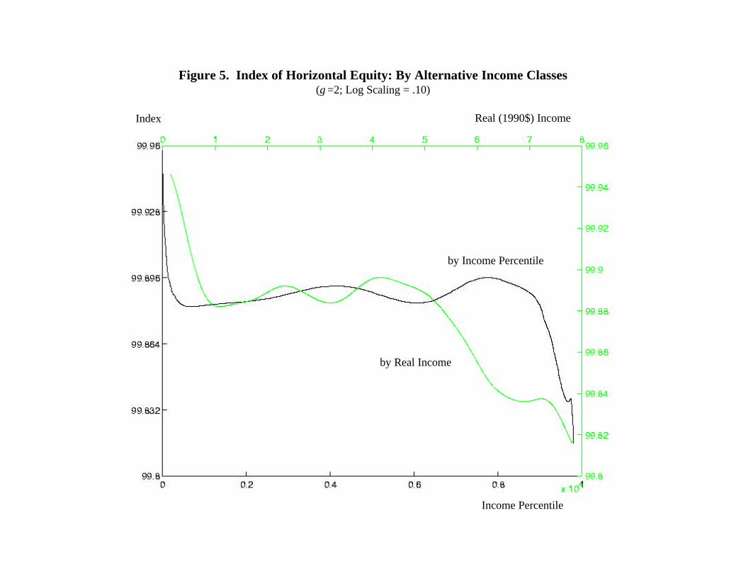
Figure 5. Index of Horizontal Equity: By Alternative Income Classes(γ =2; Log Scaling = .10)

Index

Income Percentile

Real (1990$) Income

by Real Income

by Income Percentile

Figure 6. Index of Horizontal Equity: Alternative Equivalence Scales(γ = .5,2, 5; Log Scaling = .10)

Income Percentile

Index

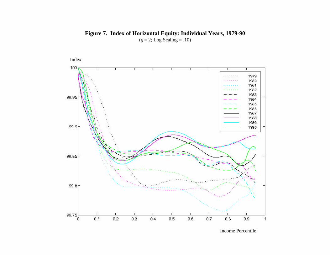
Figure 7. Index of Horizontal Equity: Individual Years, 1979-90(γ = 2; Log Scaling = .10)

Income Percentile

Index

Figure 8. Index of Horizontal Equity: 1994(γ = .5, 2; Log Scaling = .10)

Income Percentile

Index

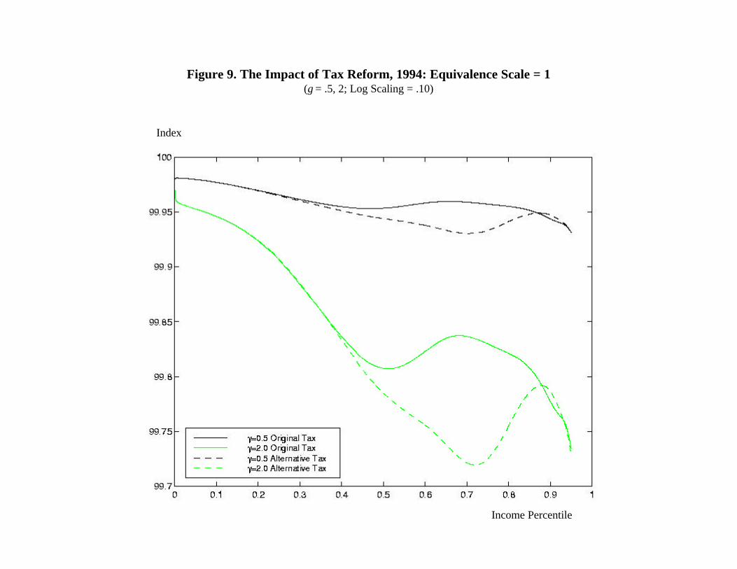
Figure 9. The Impact of Tax Reform, 1994: Equivalence Scale = 1(γ = .5, 2; Log Scaling = .10)

Income Percentile

Index

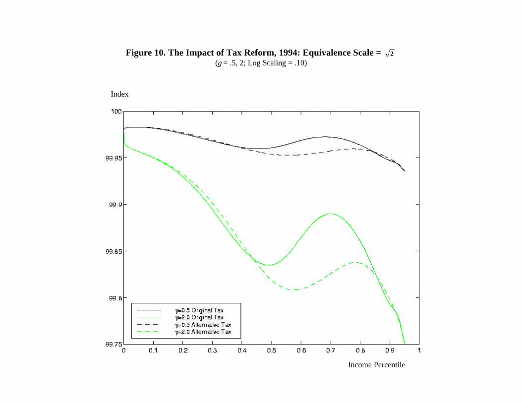
Figure 10. The Impact of Tax Reform, 1994: Equivalence Scale = 2(γ = .5, 2; Log Scaling = .10)

Income Percentile

Index

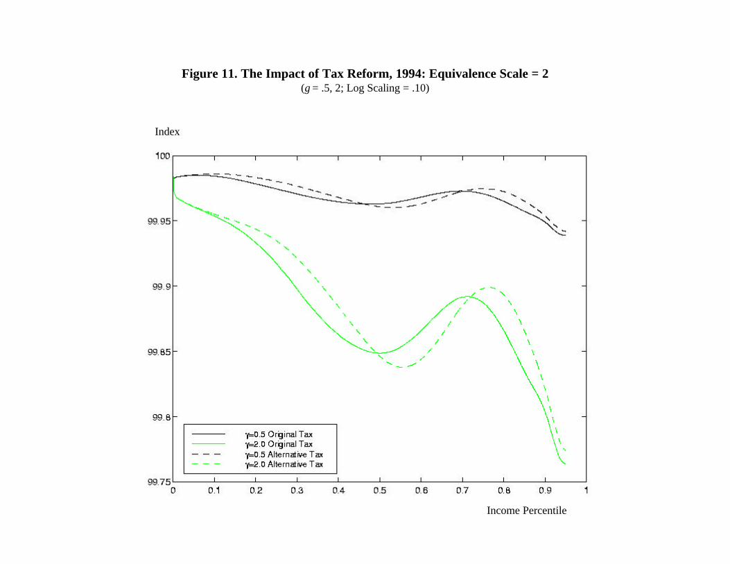
Figure 11. The Impact of Tax Reform, 1994: Equivalence Scale = 2(γ = .5, 2; Log Scaling = .10)

Income Percentile

Index

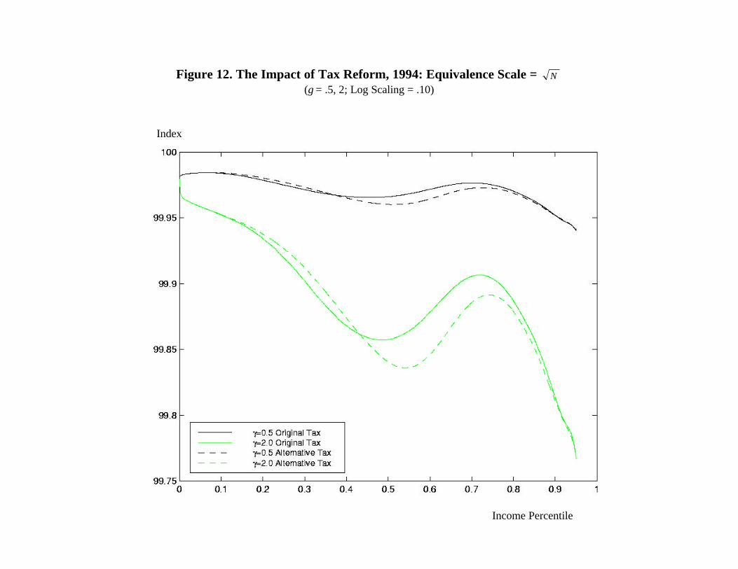
Figure 12. The Impact of Tax Reform, 1994: Equivalence Scale = N

(γ = .5, 2; Log Scaling = .10)

Income Percentile

Index

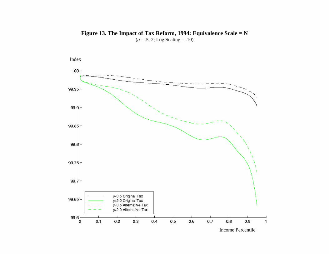
Figure 13. The Impact of Tax Reform, 1994: Equivalence Scale = N(γ = .5, 2; Log Scaling = .10)

Income Percentile

Index