Earthquake Hazard and Risk Assessment and Water-Induced Landslide Hazard
Journal ofTesting and Evaluation
M. Kayid,1 I. Elbatal,2 and F. Merovci3
DOI: 10.1520/JTE20140324
A New Family of GeneralizedQuadratic Hazard RateDistribution With Applications
VOL. 44 / NO. 4 / JULY 2016
M. Kayid,1 I. Elbatal,2 and F. Merovci3
A New Family of Generalized QuadraticHazard Rate Distribution With Applications
Reference
Kayid, M., Elbatal, I., and Merovci, F., “A New Family of Generalized Quadratic Hazard Rate Distribution
With Applications,” Journal of Testing and Evaluation, Vol. 44, No. 4, 2016, pp. 1–12, doi:10.1520/
JTE20140324. ISSN 0090-3973
ABSTRACT
The purpose of this paper is to introduce a new family of the quadratic hazard rate
distribution. This new family has the advantage of being capable of modeling various shapes
of aging and failure criteria. Furthermore, some well-known lifetime distributions such as
generalized exponential distribution, generalized linear hazard rate distribution, and
generalized Rayleigh distribution among others follow as special cases. Some statistical and
reliability properties of the new family are discussed and the maximum likelihood estimation
is used to estimate the unknown parameters. Explicit expressions are derived for the
quantiles. In addition, the asymptotic confidence intervals for the parameters are derived
from the Fisher information matrix. Finally, the obtained results are validated using a real
data set and it is shown that the new family provides a better fit than some other known
distributions.
Keywords
generalized quadratic hazard rate distribution, reliability function, order statistics, transmutation map,
maximum likelihood estimation
Introduction
Any statistical analysis depends greatly on the statistical model used to represent the phenomena
under study. Hence, the larger the class of statistical models available to the statistician, the easier
it is to choose a model. A quick survey of the models in common use reveals the abundance of sta-
tistical models in the literature. However, data of many important and practical problems do not
follow any of the probability models available. In such cases, a non-parametric model may be
Manuscript received August 23, 2014;
accepted for publication January 5,
2015.
1 Department of Statistics and Operations
Research, College of Science, King Saud
Univ., P.O. Box 2455, Riyadh 11451, KSA
(Permanent Address: Department of
Mathematics and Computer Science,
Faculty of Science, Suez Univ., Suez
41522, Egypt).
2 Institute of Statistical Studies and
Research, Department of Mathematical
Statistics, Cairo Univ., Giza, Egypt.
3 Department of Mathematics, Univ. of
Prishtina “Hasan Prishtina,” Republic of
Kosovo.
1
Journal of Testing and Evaluation
doi:10.1520/JTE20140324 / Vol. 44 / No. 4 / July 2016 / available online at www.astm.org
recommended. While a two parameters distribution may pro
vide reasonably precision in fitting data, it may be still desirable
to extend the flexibility of any distribution to allow for better
description of data without having to resort to non-parametric
models. Since there is a clear need for extended forms of these
distributions, significant progress has been made toward the
generalization of some well-known distributions and their suc
cessful applications to problems in areas such as engineering,
finance, economics, and biomedical sciences among others.
Recently, many researchers have been interested in searches
that introduce new families of distributions or generalize some
of the presented distributions which can be used to describe the
lifetimes of some devices or to describe sets of real data. An
interesting idea of generalizing a distribution, known in the
literature as transmutation, is derived by using the quadratic
rank transmutation map [1]. Based on the transmuted
generalization, various generalizations were introduced
including the transmuted Lindley distribution [2],
transmuted extreme value distribution [3], transmuted
Weibull distribution [4], transmuted additive Weibull
distribution [5], transmuted log–logistic distribution [6], and
transmuted modified Weibull distribution [7].According to
the quadratic rank transmutation map approach, the
cumulative distribution function (cdf) satisfy the relation-
shipF2ðxÞ ¼ ð1þ kÞF1ðxÞ � k F1ðxÞ
2(1)
which on differentiation yields
(2)
where f1(x) and f2(x) are the corresponding probability distribu-
tion (pdf) functions associated with cdfs F1(x) and F2(x), respec-
tively, and kj j � 1. We will use the above formulation for a
pair of distributions F(x) and G(x) where G(x) is a sub-model
of F(x). Therefore, a random variable X is said to have a trans-
muted probability distribution with cdf if
FðxÞ ¼ ð1þ kÞGðxÞ � k GðxÞ½ �2; kj j � 1
where G(x) is the cdf of the base distribution. Observe that
at k¼ 0 we have the distribution of the base random variable. On
the other hand, the quadratic hazard rate (QHR) distribution
has attracted the attention of statisticians working on theory
and methods as well as in various fields of applied statistics and
reliability. The QHR distribution may have an increasing
(decreasing) hazard rate, bathtub shaped hazard, or upside-
down bathtub shaped hazard properties. However, the QHR
distribution does not provide a reasonable parametric fit for
some practical applications. Recently, the generalized quadratic
hazard rate (GQHR) distribution was introduced and studied in
Ref. [8]. This distribution generalizes several well-known distri-
butions such as the quadratic hazard rate, the generalized linear
failure rate, the generalized exponential, and the generalized
Rayleigh distributions. In addition, the GQHR distribution may
have an increasing (decreasing) hazard function, a bathtub
shaped hazard function, or an upside-down bathtub shaped
hazard function, which provide many applications in several
areas such as reliability, life testing, and survival analysis.
However, some data of many important and practical problems
do not follow this distribution. As a result, there is a clear need
to extend the class of this distribution to a large one in order to
provide successful applications to problems in areas such as
reliability engineering and economics.
In this article, we use the transmutation map approach sug-
gested by Ref. [1] to propose a new family of life distributions
called transmuted generalized quadratic hazard rate (TGQHR)
distribution. This new family has the advantage of being capable
of modeling various shapes of aging and failure criteria. Fur-
thermore, some well-known lifetime distributions such as gen-
eralized exponential distribution, generalized linear hazard rate
distribution, and generalized Rayleigh distribution among
others are special cases of this family. The rest of the paper is
organized as follows. In the section “Density and Hazard Rate
of the New Family,” the pdf and cdf of the subject distribution
and some special sub-models are derived. In that section, some
reliability properties are discussed. In the section “Statistical
Properties,” the statistical properties including quantiles,
moments, and moment generating function, etc., are studied. In
the section “Maximum Likelihood Estimators,” we demonstrate
the maximum likelihood estimates and the asymptotic confi-
dence intervals of the unknown parameters. In the
“Applications” section, we provide some applications in the
context of reliability. The final section concludes the paper with
some remarks related to the current research. Throughout the
paper, all the integrals and the expectations are assumed to exist
when they appear.
Density and Hazard Rate of the
New Family
In this section, we study some mathematical properties of the
new family. The pdf and cdf of the subject distribution and
some special sub-models are derived. We investigate the shapes
of the density and hazard rate function. Formally, let X follow
the GQHRD with four parameters a, h, b, and l if it has the
cumulative distribution function
Fðx; a; h;b; lÞ ¼ 1� exp �gða; h;bÞf g½ �l; x > 0(3)
where:
gða; h;bÞ ¼ ax þ h2 x
2 þ b3 x
3, and
a� 0, b� 0, l� 0 and h � �2ffiffiffiffiffiffiabp
.
This restriction on the parameter space is made to assure
that the hazard function with the following form is positive
A(x, a, h, b)¼ aþ hxþ bx2, x> 0 [9]. The pdf is given by
Journal of Testing and Evaluation2
f2ðxÞ ¼ f1ðxÞ½ð1þ kÞ � 2kF1ðxÞ�
f ðx; a; h;b; lÞ¼ Uðx; a; h; b;lÞ 1� exp �gða; h; bÞf g½ �l�1; x > 0(4)
where
Uðx; a; h;b;lÞ ¼ lAðx; a; h; bÞ exp � ax þ h2 x
2 þ b3 x
3h in o
:
Substituting Eq 3 in Eq 1, we get a new family called
TGQHR distribution with cdf as
FðxÞ ¼ 1� gða; h;bÞ½ �l 1þ k� k 1� exp �gða; h; bÞf g½ �l½ �(5)
The corresponding pdf of the TGQHR is given by f
ðxÞ ¼ Uðx; a; h;b;lÞ 1� gða; h;bÞ½ �l�1
� 1þ k� 2k 1� exp �gða; h; bÞf gÞ½ �l½ �(6)
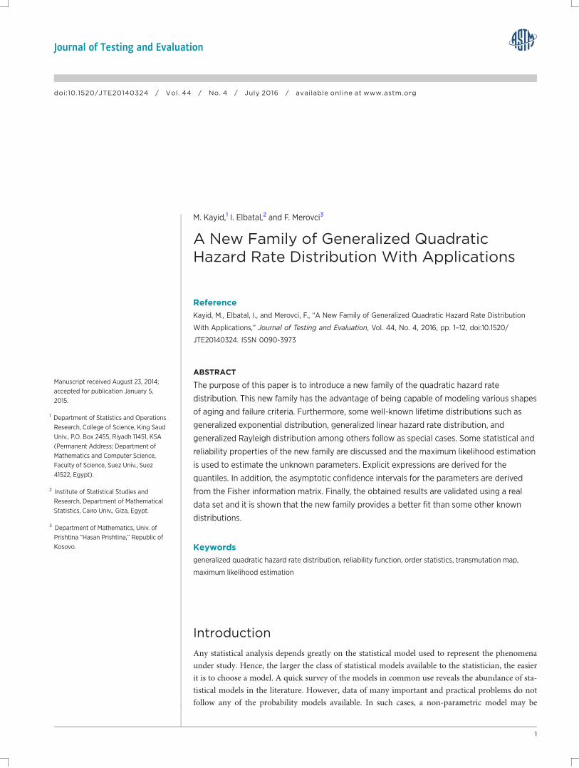
Figure 1 illustrates some of the possible shapes of the pdf
of the TGQHR distribution for selected values of the parameters:
k¼�0.9, � 0.8, � 0.7, � 0.6, � 0.5, and � 0.4; l¼ 2.6, 2.5, 2.4,
2.3, 2.2, 2.1, and 2 with color shapes purple, blue, pink, red,
green, yellow, and black, respectively. From Fig. 1, it can be seen
that the distribution of TGQHR distribution is bimodal.
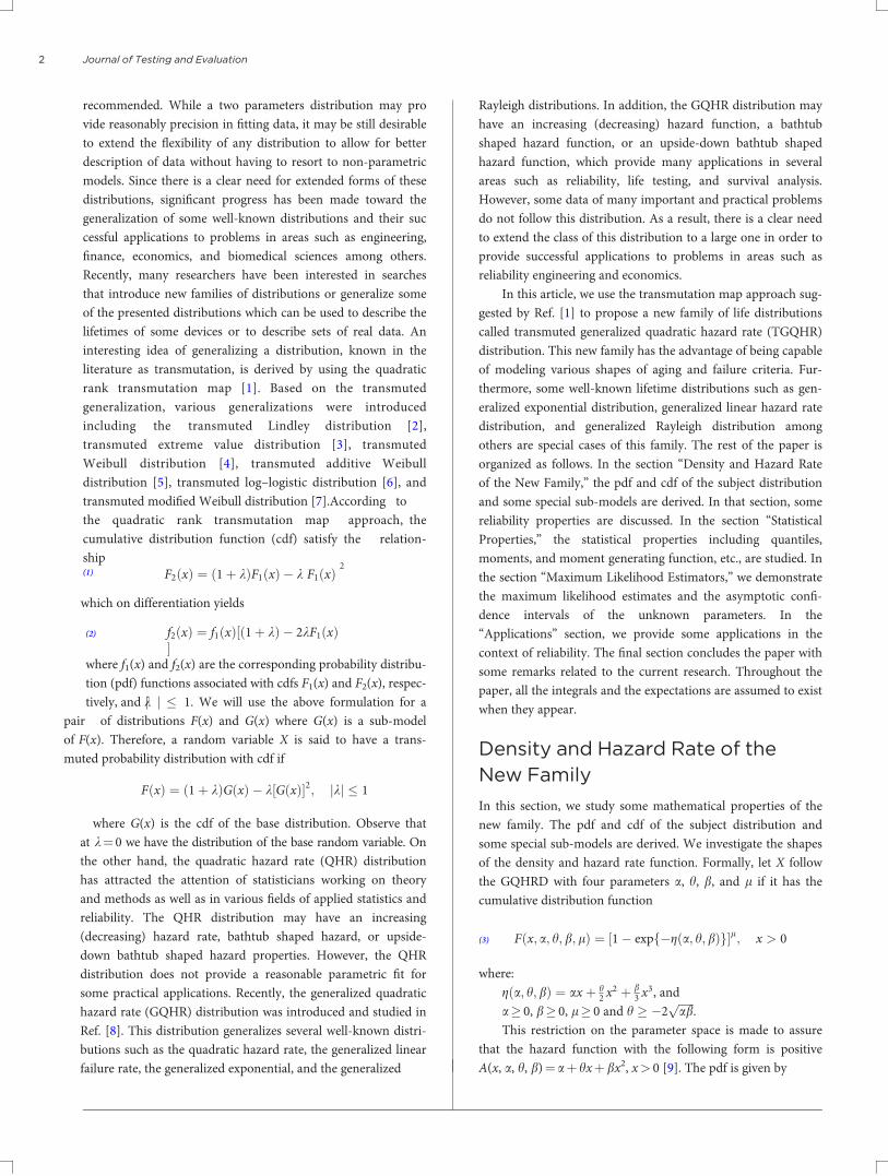
Figure 2 illustrates some of the possible shapes of the cdf of
the TGQHR distribution for selected values of the parameters for
values of parameters: k¼�0.9, � 0.8, � 0.7, � 0.6, � 0.5, and �0.4; l¼ 2.6, 2.5, 2.4, 2.3, 2.2, 2.1, and 2 with color shapes purple,
blue, pink, red, green, yellow, and black, respectively.
The TGQHR family is a very flexible model that approaches
to different distributions when its parameters are changed. The
following example shows that the new family is very flexible
and generalizes some well-known distributions.
EXAMPLE 2.1
Let X � TGQHR (a, h, b, l, k). Then
(1) If k¼ 0, we get generalized quadratic hazard ratedistribution.
(2) If b¼ 0, we get transmuted generalized linear hazardrate distribution.
(3) If b¼ 0 and l¼ 1, we get transmuted linear hazard (fail-ure) rate distribution.
(4) If k¼ b¼ 0, we get generalized linear hazard ratedistribution.
(5) If k¼ b¼ 0 and l¼ 1 we get linear hazard (failure) ratedistribution.
(6) If h¼ b¼ 0, we get transmuted generalized exponentialdistribution.
(7) If h¼ b¼ k¼ 0, we get generalized exponentialdistribution.
(8) If a¼ b¼ 0, we get transmuted generalized Rayleighdistribution.
(9) If a¼ b¼ k¼ 0, we get generalized Rayleighdistribution.
The TGQHR family can be a useful characterization of the
lifetime data analysis. The reliability function of the TGQHR
family is given by
RðxÞ ¼ 1� 1� exp �gða; h;bÞf g½ �l
� 1þ k� k 1� exp �gða; h;bÞf g½ �l½ �(7)
and the hazard rate function given by
hðxÞ ¼ Wða; h; b;l; kÞ � Kða; h;b;lÞ� 1þ k� 2k 1� exp �gða; h;bÞf g½ �l½ �(8)
FIG. 1 The pdfs of various TGQHR distributions.
FIG. 2 The cdfs of various TGQHR distributions.
KAYID ET AL. ON A NEW FAMILY OF GQHR DISTRIBUTION 3
where
Wða; h;b; l; kÞ ¼ ½1� 1� exp �gða; h; bÞf gÞ½ �l
� 1þ k� k 1� exp �gða; h; bÞf g½ �l½ ���1
and
Kða; h;b;l; kÞ ¼ lAðx; a; h; bÞ exp �gða; h; bÞf g� 1� exp �gða; h; bÞf g½ �l�1
It is important to note that the units for h(x) represent the
probability of failure per unit of time, distance, or cycles. These
failure rates are defined with different choices of parameters.
The cumulative hazard function of the TGQHR distribution is
given by
HðxÞ ¼ � ln j½1� exp �gða; h;bÞf g�l
� 1þ k� k½1� exp �gða; h; bÞf g½ �l�j(9)
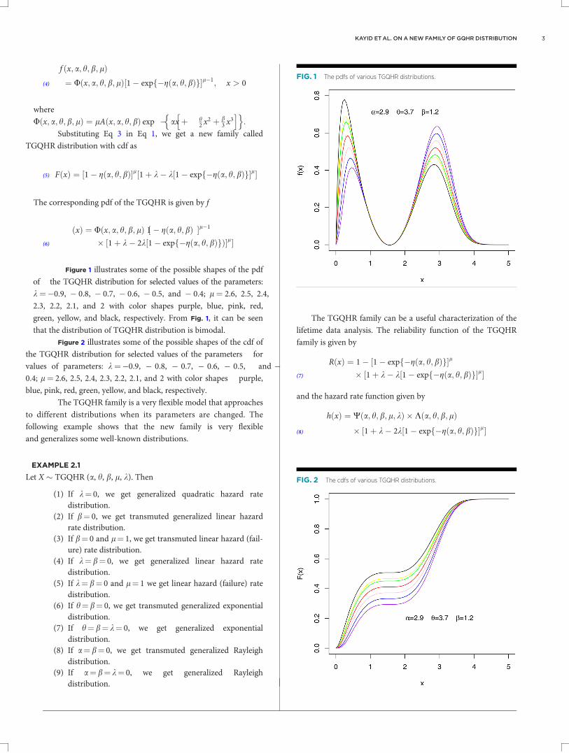
Figure 3 illustrates some of the possible shapes of the hazardrate of the TGQHR distribution for selected values of theparameters for values of parameters k ¼�0.9, �0.8, �0.7, �0.6,�0.5, and �0.4; l¼ 2.6, 2.5, 2.4, 2.3, 2.2, 2.1, and 2 with color
shapes purple, blue, pink, red, green, yellow, and black,
respectively.
Statistical Properties
In this section, we discuss some statistical properties of the new
family. Moments are necessary and important in any statistical
analysis, especially in applications. They can be used to study
the most important features and characteristics of a distribution
(e.g., tendency, dispersion, skewness, and kurtosis).
THEOREM 3.1
Let X has the TGQHR (a, h, b, l, k) with kj j � 1. Then the rth
moment of X is given as
l0r ¼ l
(ð1þ kÞni;k;m
"aCðr þ 2kþ 3mþ 1Þ
aðiþ 1Þ½ �rþ2kþ3mþ1
þ hCðr þ 2kþ 3mþ 2Þaðiþ 1Þ½ �rþ2kþ3mþ2
þ bCðr þ 2kþ 3mþ 3Þaðiþ 1Þ½ �rþ2kþ3mþ3
#
� 2k.j;k;maCðr þ 2kþ 3mþ 1Þ
aðjþ 1Þ½ �rþ2kþ3mþ1
"
þ hCðr þ 2kþ 3mþ 2Þaðjþ 1Þ½ �rþ2kþ3mþ2
þ bCðr þ 2kþ 3mþ 3Þaðjþ 1Þ½ �rþ2kþ3mþ3
#)
(10)
where
ni;k;m ¼X
ii; k;m ¼ 01
l� 1� �
ð�1Þiþkþm ðiþ 1Þkþmhkbm
2k3mk!m!
and
.j;k;m ¼X
i; k;m ¼ 012l� 1
j
� �ð�1Þjþkþm ðiþ 1Þkþmhkbm
2k3mk!m!
PROOF
First, we have
l0r ¼ lð10xrAðx;a; h;bÞgða; h;bÞ 1� gða;h;bÞ½ �l�1
� 1þ k� 2k 1� gða;h;bÞ½ �l½ �dx
¼ l ð1þ kÞð10xrAðx; a; h;bÞgða;h;bÞ 1� gða; h;bÞ½ �l�1
�dx
� 2kð10xrAðx; a;h;bÞgða;h;bÞ 1� gða; h;bÞ½ �2l�1dx
�
193Since 0< g (a, h, b)< 1, then by using the following facts that
1� gða; h; bÞ½ �l�1¼X1i¼0ð�1Þi l� 1
i
� �exp �igða; h;bÞf g
194and
1� gða; h; bÞ½ �2l�1¼X1j¼0ð�1Þj 2l� 1
j
� �exp �jgða; h;bÞf g
(11)
FIG. 3 The hazards of various TGQHR distributions.
Journal of Testing and Evaluation4
we have l0r
¼ lX1i¼0ð�1Þi
l� 1
i
( � �ð1þ kÞ
ð10xrAðx; a; h;bÞ
� exp � ðiþ 1Þgða; h; bÞ½ �f gdx � 2kX1j¼0ð�1Þj
2l� 1
j
� �
�ð10xrAðx; a; h; bÞ exp � ðjþ 1Þgða; h;bÞ½ �f gdx
�(12)
Notice that the expansion of exp �ðiþ 1Þ h2 x
2� �
and
exp �ðiþ 1Þ b3 x
3h i
are given, respectively, by
exp �ðiþ 1Þ h2x2
¼X1k¼0
�ðiþ 1Þ h2x2
kk!
(13)
and
exp �ðiþ 1Þ b3x3
¼X1m¼0
�ðiþ 1Þ b3x3
mm!
(14)
Now, substituting from Eqs 12–13, we have l0r
¼ l ni;k;m a( " ð10xrþ2kþ3m exp �aðiþ
1Þx f
gdx
þ hð10xrþ2kþ3mþ1 exp �aðiþ 1Þxf gdx
þ bð10xrþ2kþ3mþ2 exp �aðiþ 1Þxf gdx
� 2k.j;k;m að10xrþ2kþ3m exp �aðjþ 1Þxf gdx
þ hð10xrþ2kþ3mþ1 exp �aðjþ 1Þxf gdx
þ bð10xrþ2kþ3mþ2 exp �aðjþ 1Þxf gdx
#)
¼ l
(ni;k;m
"aCðr þ 2kþ 3mþ 1Þ
aðiþ 1Þ½ �rþ2kþ3mþ1
þ hCðr þ 2kþ 3mþ 2Þaðiþ 1Þ½ �rþ2kþ3mþ2
þ bCðr þ 2kþ 3mþ 3Þaðiþ 1Þ½ �rþ2kþ3mþ3
#
� 2k.j;k;maCðr þ 2kþ 3mþ 1Þ
aðjþ 1Þ½ �rþ2kþ3mþ1
"
þ hCðr þ 2kþ 3mþ 2Þaðjþ 1Þ½ �rþ2kþ3mþ2
þ bCðr þ 2kþ 3mþ 3Þaðjþ 1Þ½ �rþ2kþ3mþ3
#)
which completes the proof.
Based on Theorem 3.1, the measures of variation, skewness,
and kurtosis of the TGQHR distribution can be obtained
according to the following relation
CV ¼ffiffiffiffiffiffiffiffiffiffiffiffiffil2
l1� 1
r
CS ¼ l3ðhÞ � 3l1ðhÞl2ðhÞ þ 2l31ðhÞ
l2ðhÞ � l21ðhÞ½ �
32
and
CK ¼ l4ðhÞ � 4l1ðhÞl3ðhÞ þ 6l21ðhÞl2ðhÞ � 3l4
1ðhÞl2ðhÞ � l2
1ðhÞ½ �2
In the next result, we derived the moment generating func-
tion (mgf) of the new family.
THEOREM 3.2
If X has the TGQHR (a, h, b, l, k) with kj j � 1, then the mgf of
X is given as follows:
MXðtÞ ¼ l
(ð1þ kÞni;k;m
aCð2kþ 3mþ 1Þaðiþ 1Þ � t½ �2kþ3mþ1
þ hCð2kþ 3mþ 2Þaðiþ 1Þ � t½ �2kþ3mþ2
þ bCð2kþ 3mþ 3Þaðiþ 1Þ � t½ �2kþ3mþ3
� 2k.j;k;maCð2kþ 3mþ 1Þ
aðjþ 1Þ � t½ �2kþ3mþ1þ hCð2kþ 3mþ 2Þ
aðjþ 1Þ � t½ �2kþ3mþ2
þ bCð2kþ 3mþ 3Þaðjþ 1Þ � t½ �2kþ3mþ3
)
PROOF
We have
MXðtÞ ¼ l
�ð1þ kÞ
ð10
hetx aþ hx þ bx2� �
gða; h; bÞ
� 1� gða; h; bÞ½ �l�1idx � 2k
ð10etxðaþ hx þ bx2Þ
� gða; h;bÞ 1� gða; h;bÞ½ �2l�1dx�
(15)
Substituting Eqs 11 and 13 into the relation in Eq 15, we get the
following:
MXðtÞ ¼ l
�ð1þ kÞni;k;m
ð10x2kþ3mAðx; a; h;bÞ
� exp �ðaðiþ 1Þ � tÞxf gdx � 2k.j;k;m
�ð10x2kþ3mAðx; a; h;bÞ exp � aðjþ 1Þ � t½ �xf gdx
�
¼ l
�ð1þ kÞni;k;m
aCð2kþ 3mþ 1Þ
aðiþ 1Þ � t½ �rþ2kþ3mþ1
þ hCð2kþ 3mþ 2Þaðiþ 1Þ � t½ �rþ2kþ3mþ2
þ bCð2kþ 3mþ 3Þaðiþ 1Þ � t½ �rþ2kþ3mþ3
� 2k.j;k;m
aCð2kþ 3mþ 1Þ
aðjþ 1Þ � t½ �rþ2kþ3mþ1
þ hCð2kþ 3mþ 2Þaðjþ 1Þ � t½ �rþ2kþ3mþ2
þ bCð2kþ 3mþ 3Þaðjþ 1Þ � t½ �rþ2kþ3mþ3
�
which completes the proof.
KAYID ET AL. ON A NEW FAMILY OF GQHR DISTRIBUTION 5
Research in the area of order statistics has been steadily and
rapidly growing, especially during the last two decades. The
extensive role of order statistics in several areas of statistical
inference has made it imperative and useful, and together these
results are presented in a varied manner to suit diverse interests.
Let X1, X2,…, Xn be a simple random sample from TGQHR (a,
h, b, l, k) with cumulative distribution function and probability
density function as in Eqs 5 and 6, respectively. Let X(1)�X(2)
�…� X(n) denote the order in which statistics were obtained
from this sample. In reliability literature, X(i) denote the lifetime of
an (n – iþ 1) out-of-n system, which consists of n independent and
identically components. Then the pdf of X(i), 1� i� n 227 is given
by
fi::nðxÞ ¼
1bði; n� iþ 1Þ Fðx; �Þ½ �i�1 1� Fðx; �Þ½ �n�if ðx; �Þ
where �¼ a, h, b, l, k.
In addition, the joint pdf of X(i:n), X(j:n) and 1� i� j� n is
fi:j:nðxi; xjÞ ¼ w FðxiÞ½ �i�1 FðxjÞ � FðxiÞ� �j�i�1
� 1� FðxjÞ� �n�j
f ðxiÞf ðxjÞ
where w ¼ n!ði�1Þ!ðj�i�1Þ!ðn�jÞ! :
Let X1, X2,…,Xn be independently and identically distrib-
uted order random variables from the TGQHR distribution
having first, last, and median order pdfs given by the following
f1:nðxÞ ¼ n 1� Fðx; �Þ
½ �n�1f ðx; �Þ¼ n 1� ð1� hð1ÞÞl 1þ k� kð1� hð1ÞÞl
� �� �n�1� lðaþ hxð1Þ þ bx2ð1ÞÞhð1Þð1� hð1ÞÞl�1
� 1þ k� 2kð1� hð1ÞÞl� �
fn:nðxÞ ¼ n FðxðnÞ; �Þ� �n�1
f ðxðnÞÞ; �Þ
¼ n ð1� hðnÞÞl 1þ k� kð1� hðnÞÞl� �� �n�1
� lðaþ hxðnÞ þ bx2ðnÞÞhðnÞð1� hðnÞÞl�1
� 1þ k� 2kð1� hðnÞÞl� �
and
fmþ1:nð~xÞ ¼ð2mþ 1Þ!m!m!
Fð~xÞ½ �m 1�Fð~xÞ½ �mf ð~xÞ
¼ ð2mþ 1Þ!m!m!
1� hðmþ1Þ� �l
1þ k� kð1� hðmþ1ÞÞl� �� �m
� 1�ð1� hðmþ1Þ� �l
1þ k� kð1� hðmþ1ÞÞl� �� �m
�lðaþ hxðmþ1Þ þbx2ðmþ1ÞÞhðmþ1Þð1� hðmþ1ÞÞl�1
� 1þ k� 2kð1� hðmþ1ÞÞl� �
where hðiÞ ¼ exp � axðiÞ þ h2 x
2ðiÞ þ
b3 x
3ðiÞ
h in o.
The joint distribution of the ith and jth order statistics from
transmuted generalized quadratic hazard rate distribution is
fi:j:nðxi; xjÞ ¼ w FðxiÞ½ �i�1 FðxjÞ � FðxiÞ� �j�i�1
� 1� FðxjÞ� �n�j
f ðxiÞf ðxjÞ
¼ w ð1� hðiÞÞl 1þ k� kð1� hðiÞÞl� �� �i�1
� ð1� hðjÞÞl 1þ k� kð1� hðjÞÞl� ��
�ð1� hðiÞÞl 1þ k� kð1� hðiÞÞl� ��j�i�1
� 1� ð1� hðjÞÞl 1þ k� kð1� hðjÞÞl� �� �n�j
� lðaþ hxðiÞ þ bx2ðiÞÞhðiÞð1� hðiÞÞl�1
� 1þ k� 2kð1� hðiÞÞl� �
lðaþ hxðjÞ þ bx2ðjÞÞ
� hðjÞð1� hðjÞÞl�1 1þ k� 2kð1� hðjÞÞl� �
If i¼ 1 and j¼ n, we get the joint distribution of the minimum
and maximum of order statistics
f1::n:nðxi; xjÞ ¼ nðn� 1Þ FðxðnÞÞ � Fðxð1ÞÞ� �n�2
f ðxð1ÞÞf ðxðnÞÞ
¼ nðn� 1Þ ð1� hðnÞÞl 1þ k� kð1� hðnÞÞl� ��
�ð1� hð1ÞÞl 1þ k� kð1� hð1ÞÞl� ��n�2
� lðaþ hxð1Þ þ bx2ð1ÞÞhð1Þð1� hð1ÞÞl�1
� 1þ k� 2kð1� hð1ÞÞl� �
lðaþ hxðnÞ þ bx2ðnÞÞ
� hðnÞð1� hðnÞÞl�1 1þ k� 2kð1� hðnÞÞl� �
Maximum Likelihood Estimators
In this section, we consider the maximum likelihood estimators
(MLEs) of TGQHR distribution. In addition, we will derive the
asymptotic interval estimates of the parameters. Let U¼ (a, h,
b, l, k)T in order to estimate the parameters a, h, b, and k of
the transmuted quadratic hazard rate distribution; let x1,…, xnbe a random sample of size n from TGQHR. Then the log likeli-
hood function can be written as
Lða; h;b; k; x ið ÞÞ ¼n
logl½ ��1þXni¼1
ln aþ hxðiÞ þ bx2ðiÞ
h i
� aXni¼1
xðiÞ �h2
Xni¼1
x2ðiÞ �b3
Xni¼1
x3ðiÞ
þ ðl� 1ÞXni¼1
ln 1� Xðx; a; h; bÞ½ �
þXni¼1
ln 1þ k� 2k 1� Xðx; a; h;bÞ½ �l½ �
where Xðx; a; h; bÞ ¼ exp � axðiÞ þ h2 x
2ðiÞ þ
b3 x
3ðiÞ
h in o.
Differentiating L with respect to each parameter a, h, b, l,
and k, and setting the result equal to zero, we obtain maximum
likelihood estimates. The partial derivatives of L with respect to
each parameter or the score function is given by
Journal of Testing and Evaluation6
UnðUÞ ¼@L@a;@L@h;@L@b;@L@l;@L@k
� �
where the values of @L@a ;
@L@h ;
@L@b ;
@L@l ;
@L@k appeared in the
Appendix A, from Eqs A1– A5.
By solving this nonlinear system of equations (Eqs A1–A5),
these solutions will yield the ML estimators for ^ a; h; b; l, and k.
For the five parameters TGQHR (a, h, b, l, k) pdf, all the sec
ond order derivatives exist. Thus we have the inverse dispersion
matrix, which is given by
^ahb^lk
0BBBBBB@
1CCCCCCA � N
ahblk
0BBBBBB@
1CCCCCCA;
Vaa Vah Vab Val Vak
Vha Vhh Vhb Vhl Vhk
Vba Vbh Vbb Vbl Vbk
Vla Vlh Vlb Vll Vlk
Vka Vkh Vkb Vkl Vkk
0BBBBBBB@
1CCCCCCCA
266666664
377777775
V�1 ¼ �EVaa Vah Vab Val Vak
Vka Vkh Vkb Vkl Vkk
where
Vaa ¼@2L@a2
; Vhh ¼@2L
@h2; Vbb ¼
@2L
@b2 ;
Vaa ¼@2L@l2
; Vkk ¼@2L
@k2
and
Vah ¼@2L@a@h
; Vka ¼@2L@a@k
; Vbk ¼@2L@b@k
; Vbl ¼@2L@b@l
The values of Vll, Vaa, Vhh, Vbb, Vkk, Vah, Vka, Vbk, Vbl, Vab,
Vbh, Vlh, and Vkh appeared in Appendix B.
By solving this inverse dispersion matrix, these solutions
will yield asymptotic variance and covariances of these ML estimators
for ^ a, h; b; l, and k. We approximate 100(1 – c)% confi-
dence intervals for a, b, h, and k are determined, respectively, as
a 6 zc2
ffiffiffiffiffiffiffiVaa
q; h 6 zc
2
ffiffiffiffiffiffiffiVhh
q; b 6 zc
2
ffiffiffiffiffiffiffiffiVbb
q;
l 6 zc2
ffiffiffiffiffiffiffiffiVll
q; k 6 zc
2
ffiffiffiffiffiffiffiffiVkk
q
where zc is the upper 100cthe percentile of the standard normal
distribution.
We can compute the maximized unrestricted and restricted
log-likelihood functions to construct the likelihood ratio (LR)
test statistic for testing on some transmuted GQHR sub-models.
For example, we can use the LR test statistic to check whether
the TGQHR distribution for a given data set is statistically supe-
rior to the GQHR distribution. In any case, hypothesis tests of
the type H0: h¼ h0 versus H0: h= h0 can be performed using a
LR test. In this case, the LR test statistic for testing H0 versus H1
is x ¼ 2�‘ðh; xÞ � ‘ðh0; xÞ
�, where h and h0 are the MLEs
under H1 and H0, respectively. The statistic x is asymptotically
(as n !1) distributed as v2k, where k is the length of the pa-
rameter vector h of interest. The LR test rejects H0 if x > v2k;c,
where v2k;c denotes the upper 100c% quantile of the v2kdistribution.
Applications
In this section, we use real data sets to show that the TGQHR
distribution can be a better model than one based on the
GQHR distribution. The data set studied in Ref. [1] gives the
times of failure and running times for a sample of devices
from an eld-tracking study of a larger system. At a certain
point in time, 30 units were installed in normal service condi-
tions. Two causes of failure were observed for each unit that
failed: the failure caused by an accumulation of randomly
occurring damage from power-line voltage spikes during elec-
tric storms and failure caused by normal product wear. The
times divided by 100 are: 2.75, 0.13, 1.47, 0.23, 1.81, 0.30,
0.65, 0.10, 3.00, 1.73, 1.06, 3.00, 3.00, 2.12, 3.00, 3.00, 3.00,
0.02, 2.61, 2.93, 0.88, 2.47, 0.28, 1.43, 3.00, 0.23, 3.00, 0.80,
2.45, and 2.66.
The variance covariance matrix of the MLEs under the
TGQHR distribution is computed as
IðhÞ�1 ¼
0:017729324 �0:03011476 0:03564007 �0:02444729 �0:009815549
�0:030114761 0:33179665 �0:40133555 0:26590729 0:112121322
0:035640069 �0:40133555 0:55756796 �0:30675306 �0:176577320
�0:024447287 0:26590729 �0:30675306 0:44567201 0:083699256
�0:009815549 0:11212132 �0:17657732 0:08369926 0:062454042
0BBBBBBBBBBBB@
1CCCCCCCCCCCCA
Thus, the variances of the MLE of k, a, h, l,
and b are Varð kÞ¼0:017729324; VarðaÞ¼0:33179665; VarðhÞ¼0:55756796; VarðlÞ¼0:55756796, and VarðbÞ¼0:062454042.
Therefore, 95 % confidence intervals for k, a, h, l, and b
are [�0.7369934, �1], [1.790662, 4.048652], [�5.197785,�2.270703], [1.292003, 3.908943], and [0.7854041, 1.765044].
The variance covariance matrix of the MLEs under the GQHR
distribution is computed as
KAYID ET AL. ON A NEW FAMILY OF GQHR DISTRIBUTION 7
IðhÞ�1
¼
0:3137415 �0:4046424 0:20696569 0:12129517
�0:4046424 0:5644128 �0:25747681 �0:179952270:2069657 �0:2574768 0:20641582 0:07713621
0:1212952 �0:1799523 0:07713621 0:06139265
0BBBB@
1CCCCA
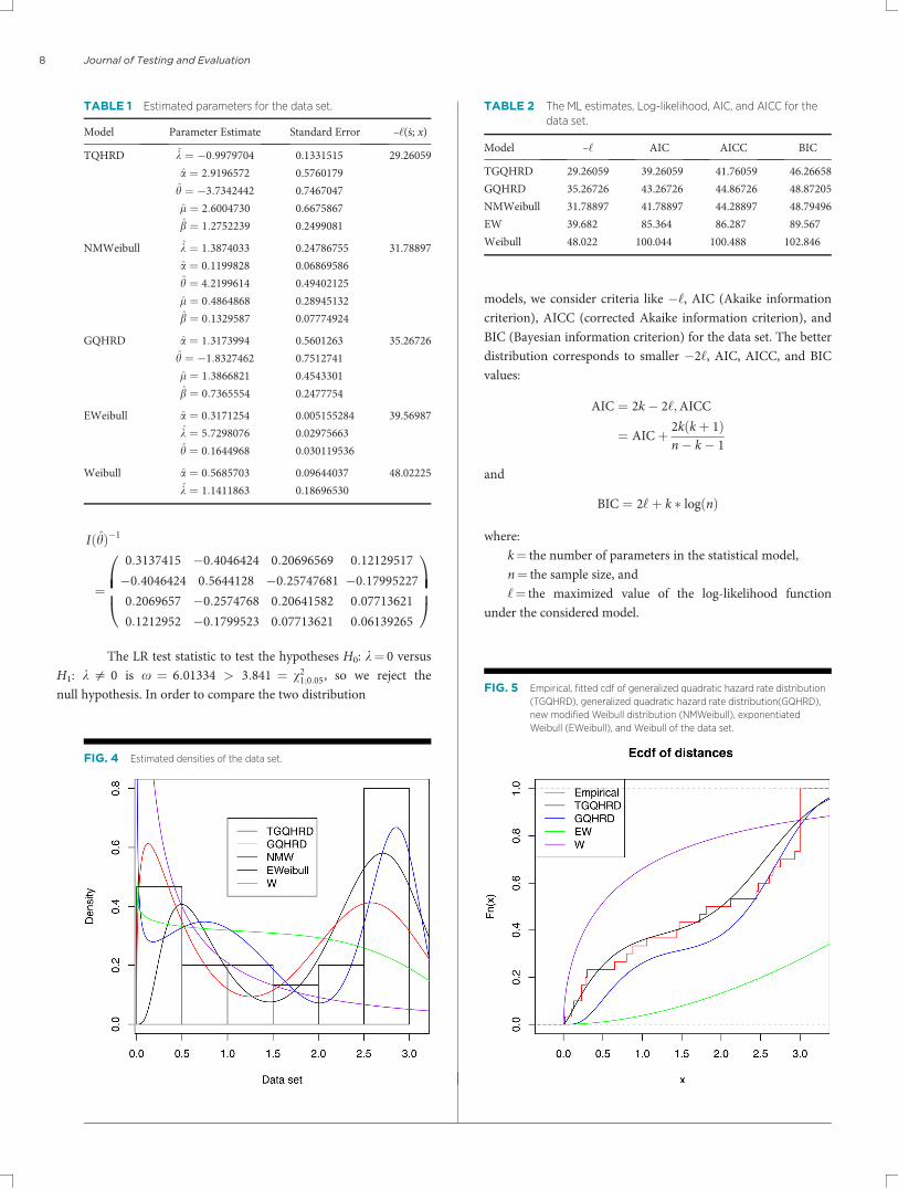
The LR test statistic to test the hypotheses H0: k¼ 0 versus
H1: k = 0 is x ¼ 6:01334 > 3:841 ¼ v21;0:05, so we reject the
null hypothesis. In order to compare the two distribution
models, we consider criteria like �‘, AIC (Akaike information
criterion), AICC (corrected Akaike information criterion), and
BIC (Bayesian information criterion) for the data set. The better
distribution corresponds to smaller �2‘, AIC, AICC, and BIC
values:
AIC ¼ 2k� 2‘;AICC
¼ AICþ 2kðkþ 1Þn� k� 1
and
BIC ¼ 2‘þ k � logðnÞ
where:
k¼ the number of parameters in the statistical model,
n¼ the sample size, and
‘¼ the maximized value of the log-likelihood function
under the considered model.
FIG. 4 Estimated densities of the data set.
TABLE 2 The ML estimates, Log-likelihood, AIC, and AICC for the
data set.
Model –‘ AIC AICC BIC
TGQHRD 29.26059 39.26059 41.76059 46.26658
GQHRD 35.26726 43.26726 44.86726 48.87205
NMWeibull 31.78897 41.78897 44.28897 48.79496
EW 39.682 85.364 86.287 89.567
Weibull 48.022 100.044 100.488 102.846
TABLE 1 Estimated parameters for the data set.
Model Parameter Estimate Standard Error –‘(s; x)
TQHRD k ¼ �0:9979704 0.1331515 29.26059
a ¼ 2:9196572 0.5760179
h ¼ �3:7342442 0.7467047
l ¼ 2:6004730 0.6675867
b ¼ 1:2752239 0.2499081
NMWeibull k ¼ 1:3874033 0.24786755 31.78897
a ¼ 0:1199828 0.06869586
h ¼ 4:2199614 0.49402125
l ¼ 0:4864868 0.28945132
b ¼ 0:1329587 0.07774924
GQHRD a ¼ 1:3173994 0.5601263 35.26726
h ¼ �1:8327462 0.7512741
l ¼ 1:3866821 0.4543301
b ¼ 0:7365554 0.2477754
EWeibull a ¼ 0:3171254 0.005155284 39.56987
k ¼ 5:7298076 0.02975663
h ¼ 0:1644968 0.030119536
Weibull a ¼ 0:5685703 0.09644037 48.02225
k ¼ 1:1411863 0.18696530
FIG. 5 Empirical, fitted cdf of generalized quadratic hazard rate distribution
(TGQHRD), generalized quadratic hazard rate distribution(GQHRD),
new modified Weibull distribution (NMWeibull), exponentiated
Weibull (EWeibull), and Weibull of the data set.
Journal of Testing and Evaluation8
Table 1 below provide the estimated parameters of the
TGQHRD, GQHRD, new modified Weibull [10], exponentiated
Weibull, and Weibull distribution for the data set. See Fig. 4.
Maximum likelihood estimation is used to estimate param-
eters for the fitted models. The values of estimated parameters with
standard error and negative log-likelihood are given in Table 1.
According to negative log-likelihood criterion, it can be seen from
Table 1 that the proposed model is a superior model
for goodness of fit.
Table 2 shows the values of �2log (L), AIC, and AICC for
the five fitted distributions for the data set.
The values in Table 2 indicate that the TGQHR is a strong
competitor to other distribution used here for the fitting data set.
A density plot compares the fitted densities of the models with
the empirical histogram of the observed data. The fitted density
for the TGQHR model is closer to the empirical histogram than the
fits of the GQHR model. See Fig. 5.
Conclusion
In the present study, we introduced a new family of generalized
quadratic hazard rate distributions. The subject family is gener-
ated by using the quadratic rank transmutation map and taking
the generalized quadratic hazard rate distribution as the base
distribution. Some statistical and reliability properties along
with estimation issues are addressed. The hazard rate function
and reliability behavior of the new family shows that the subject
family can be used to model reliability data. We expect that this
study will serve as a reference and help to advance future
research in the subject area.
ACKNOWLEDGMENTS
The writers would like to thank two reviewers for their valuable
comments and suggestions, which were helpful in improving the
paper. This work was supported by King Saud University, Dean
ship of Scientific Research, College of Science Research Center.
Appendix A
The values of @L@a ;
@L@h ;
@L@b ;
@L@l, and
@L@k are as follows:
@L@l¼ n
lþXni¼1
ln 1� Xðx; a; h;bÞ½ �
� 2kXni¼1
1� Xðx; a; h;bÞ½ �llog 1� Xðx; a; h;bÞ½ �1þ k� 2k 1� Xðx; a; h;bÞ½ �l½ � ¼ 0
(A1)
@L@a¼Xni¼1
1
aþ hxðiÞ þ bx2ðiÞ
h i�X
i ¼ 1nxðiÞðl� 1ÞXni¼1
xðiÞXðx; a; h; bÞ1� Xðx; a; h;bÞ½ �
þ 2klXni¼1
xðiÞXðx; a; h;bÞ 1� Xðx; a; h;bÞ½ �l�1
1þ k� 2k 1� Xðx; a; h;bÞ½ �l½ � ¼ 0(A2)
@ log L@h
¼Xni¼1
xðiÞðaþ hxðiÞ þ bx2ðiÞÞ
� 12
Xi ¼ 1nx2ðiÞ þ ðl� 1Þ
Xni¼1
x2ðiÞXðx; a; h;bÞ2 1� Xðx; a; h;bÞ½ �
þ klXni¼1
x2ðiÞXðx; a; h;bÞ 1� Xðx; a; h;bÞ½ �l�1
1þ k� 2k 1� Xðx; a; h;bÞ½ �l½ � ¼ 0
(A3)
@ log L@b
¼Xni¼1
x2ðiÞðaþ hxðiÞ þ bx2ðiÞÞ
� 13
Xni¼1
x3ðiÞ þ ðl� 1ÞXni¼1
x3ðiÞXðx; a; h;bÞ3 1� Xðx; a; h;bÞ½ �
þXni¼1
2kx3ðiÞXðx; a; h;bÞ 1� Xðx; a; h; bÞ½ �l�1
3 1þ k� 2k 1� Xðx; a; h;bÞ½ �l½ � ¼ 0
(A4)
@ log L@k
¼Xni¼1
1� 2 1� Xðx; a; h; bÞ½ �l
1þ k� 2k 1� Xðx; a; h;bÞ½ �l½ � ¼ 0(A5)
Appendix B
The values of Vll, Vaa, Vhh, Vbb, Vkk, Vah, Vka, Vbk, Vbl, Vab,
Vbh, Vlh, and Vkh are as follows:
Vll ¼ �nl2
� 2Xni¼1
��1� kþ 2k 1� e�axi�1=2hx2i �1=3bx3i
�l �h i�2� k 1� e�axi�1=2hx2i �1=3bx3i �l
� ln 1� e�axi�1=2hx2i �1=3bx3i � �2
1þ kð Þ�
Vaa ¼Xni¼1� aþ hxi þ bx2i� ��2
� ðl� 1ÞXni¼1
��1þ e�axi�1=2hx2i �1=3bx3ih i�2
� x2i e�axi�1=2hx2i �1=3bx3i
�þ A
where
A ¼ �2Xni¼1
�1þ e�axi�1=2hx2i �1=3bx3i �2�
� �1� kþ 2k 1� e�axi�1=2hx2i �1=3bx3i �lh i2
� k 1� e�axi�1=2hx2i �1=3bx3i �l
lx2i e�axi�1=2hx2i �1=3bx3i � A1
�
and
A1 ¼ le�axi�1=2hx2i �1=3bx3i þ le�axi�1=2hx2i �1=3bx3i k
� 1� kþ 2k 1� e�axi�1=2hx2i �1=3bx3i �l
KAYID ET AL. ON A NEW FAMILY OF GQHR DISTRIBUTION 9
Vhh ¼Xni¼1� x2i
aþ hxi þ bx2ið Þ2� ðl� 1Þ
4
�Xni¼1
x4i e�axi�1=2hx2i �1=3bx3i
�1þ e�axi�1=2hx2i �1=3bx3i� �2 � B
2
where
B ¼Xni¼1
�1þ e�axi�1=2hx2i �1=3bx3i ��2�
� �1� kþ 2k 1� e�axi�1=2hx2i �1=3bx3i �l ��2
� k 1� e�axi�1=2hx2i �1=3bx3i �l
lx4i e�axi�1=2hx2i �1=3bx3i � B1
oand
B1 ¼ le�axi�1=2hx2i �1=3bx3i þ le�axi�1=2hx2i �1=3bx3i k� 1
� kþ 2k 1� e�axi�1=2hx2i �1=3bx3i �l
Vbb ¼Xni¼1� x4i
aþ hxi þ bx2ið Þ2
� ðl� 1Þ9
Xni¼1
x6i e�axi�1=2hx2i �1=3bx3i
�1þ e�axi�1=2hx2i �1=3bx3i� �2 þ C
where
C ¼ �2=9Xni¼1
�1þ e�axi�1=2hx2i �1=3bx3i ��2�
� �1� kþ 2k 1� e�axi�1=2hx2i �1=3bx3i �lh i�2
� k 1� e�axi�1=2hx2i �1=3bx3i �l
lx6i e�axi�1=2hx2i �1=3bx3i C1
o
and
C1 ¼ le�axi�1=2hx2i �1=3bx3i þ le�axi�1=2hx2i �1=3bx3i k� 1
� kþ 2k 1� e�axi�1=2hx2i �1=3bx3i �l
Vkk ¼Xni¼1�
1� 2 1� e�axi�1=2hx2i �1=3bx3i� �lh i2
1þ k� 2k 1� e�axi�1=2hx2i �1=3bx3i� �lh i2
Vah ¼ �Xni¼1
xiaþ hxi þ bx2ið Þ2
� ðl� 1Þ2
Xni¼1
x3i e�axi�1=2hx2i �1=3bx3i
�1þ e�axi�1=2hx2i �1=3bx3i� �2 þ D
where
D ¼ � �1þ e�axi�1=2hx2i �1=3bx3ih i2�
� �1� kþ 2k 1� e�axi�1=2hx2i �1=3bx3i �lh i2
�k 1� e�axi�1=2hx2i �1=3bx3i �l
lx3i e�axi�1=2hx2i �1=3bx3i � D1
o
and
D1 ¼ le�axi�1=2hx2i �1=3bx3i þ le�axi�1=2hx2i �1=3bx3i k� 1� k
þ 2k 1� e�axi�1=2hx2i �1=3bx3i �l
Vka ¼ 2Xni¼1
1� e�axi�1=2hx2i �1=3bx3i� �l
lxie�axi�1=2hx2i �1=3bx3i
�1� kþ 2k 1� e�axi�1=2hx2i �1=3bx3i� �l �2
�1þ e�axi�1=2hx2i �1=3bx3i� �
Vbk ¼23
Xni¼1
1� e�axi�1=2hx2i �1=3bx3i� �l
lx3i e�axi�1=2hx2i �1=3bx3i
�1� kþ 2k 1� e�axi�1=2hx2i �1=3bx3i� �l �2
�1þ e�axi�1=2hx2i �1=3bx3i� �
Vbl ¼13
Xni¼1
x3i e�axi�1=2hx2i �1=3bx3i
1� e�axi�1=2hx2i �1=3bx3i� 23
Xni¼1
1� e�axi�1=2hx2i �1=3bx3i� �l
x3i e�axi�1=2hx2i �1=3bx3i k� E
�1� kþ 2k 1� e�axi�1=2hx2i �1=3bx3i� �l �2
�1þ e�axi�1=2hx2i �1=3bx3i� �
where
E ¼ �l ln 1� e�axi�1=2hx2i �1=3bx3i �
� ln 1� e�axi�1=2hx2i �1=3bx3i �
lk
� 1� kþ 2k� 1� e�axi�1=2hx2i �1=3bx3i �l
Vab ¼ �Xni¼1
x2iaþ hxi þ bx2ið Þ2
� ðl� 1Þ3
Xi ¼ 1n
� x4i e�axi�1=2hx2i �1=3bx3i
�1þ e�axi�1=2hx2i �1=3bx3i� �2 þ F
Journal of Testing and Evaluation10
where
F ¼ �2=3Xni¼1
�1þ e�axi�1=2hx2i �1=3bx3ih i2�
� �1� kþ 2k 1� e�axi�1=2hx2i �1=3bx3i �lh i2
� k 1� e�axi�1=2hx2i �1=3bx3i �l
lx4i e�axi�1=2hx2i �1=3bx3i � F1
�
and
F1 ¼ le�axi�1=2hx2i �1=3bx3i þ le�axi�1=2hx2i �1=3bx3i k
� 1� kþ 2k 1� e�axi�1=2hx2i �1=3bx3i �l
Vbh ¼ �Xni¼1
x3iaþ hxi þ bx2ið Þ2
þ l� 16
Xi ¼ 1n
� x5i e�axi�1=2hx2i �1=3bx3i
�1þ e�axi�1=2hx2i �1=3bx3i� �2 þ K
where
K ¼ �1=3Xni¼1
�1þ e�axi�1=2hx2i �1=3bx3i ��2�
� �1� kþ 2k 1� e�axi�1=2hx2i �1=3bx3i �lh i�2
� k 1� e�axi�1=2hx2i �1=3bx3i �l
lx5i e�axi�1=2hx2i �1=3bx3i � K1
�
and
K1 ¼ le�axi�1=2hx2i �1=3bx3i þ le�axi�1=2hx2i �1=3bx3i k� 1
� kþ 2k 1� e�axi�1=2hx2i �1=3bx3i �l
Val ¼Xni¼1
xie�axi�1=2hx2i �1=3bx3i
1� e�axi�1=2hx2i �1=3bx3iþ L;
where
L ¼ 2k 1� e�axi�1=2hx2i �1=3bx3i� �l
xie�axi�1=2hx2i �1=3bx3i � L1
�1þ e�axi�1=2hx2i �1=3bx3i� �
�1� kþ 2k 1� e�axi�1=2hx2i �1=3bx3i� �l �2
andL1 ¼ l ln 1� e�axi�1=2hx2i �1=3bx3i
�þ ln 1� e�axi�1=2hx2i �1=3bx3i
�lkþ 1þ k� 2k 1� e�axi�1=2hx2i �1=3bx3i
�l
Vlh ¼Xni¼1
1=2x2i e�axi�1=2hx2i �1=3bx3i
1� e�axi�1=2hx2i �1=3bx3iþ G
where
G ¼ � �1þ e�axi�1=2hx2i �1=3bx3i ��1
�1� kþ 2k 1� e�axi�1=2hx2i �1=3bx3i �l ��2
k 1� e�axi�1=2hx2i �1=3bx3i �l
x2i e�axi�1=2hx2i �1=3bx3i � G1
and
G1 ¼ �l ln 1� e�axi�1=2hx2i �1=3bx3i �
� ln 1� e�axi�1=2hx2i �1=3bx3i �
lk� 1� kþ 2k 1� e�axi�1=2hx2i �1=3bx3i �l
Vkh ¼1� e�axi�1=2hx2i �1=3bx3i� �l
lx2i e�axi�1=2hx2i �1=3bx3i
�1þ e�axi�1=2hx2i �1=3bx3i� �
�1� kþ 2k 1� e�axi�1=2hx2i �1=3bx3i� �lh i2
References
[1] Shaw, W. T. and Buckley, I. R., “The Alchemy of Probabil-ity Distributions: Beyond GramCharlier Expansions and aSkew–Kurtotic–Normal Distribution From a Rank Trans-mutation Map,” Research report, 2007.
[2] Merovci, F., “Transmuted Lindley Distribution,” IJOPCM,Vol. 6, 2013, pp. 63–72.
[3] Aryal, G. R. and Tsokos, C. P., “On theTransmuted Extreme Value Distribution WithApplication,” Nonlinear Anal. Theor., Vol. 71, 2009,pp. 1401–1407.
[4] Aryal, G. R. and Tsokos, C. P., “Transmuted WeibullDistribution: A Generalization of the Weibull ProbabilityDistribution,” Eur. J. Pure Appl. Math., Vol. 4, 2011,pp. 89–102.
KAYID ET AL. ON A NEW FAMILY OF GQHR DISTRIBUTION 11
[5] Elbatal, I. and Aryal, G. R., “On the Transmuted AdditiveWei-bull Distribution,” Aust. J. Stat., Vol. 42, 2013, pp. 117–132.
[6] Aryal, G. R., “Transmuted Log–Logistic Distribution,”J. Stat. Appl. Probab., Vol. 2, No. 1, 2013, pp. 11–20.
[7] Khan, M. S. and King, R., “Transmuted Modified WeibullDistribution: A Generalization of the Modified WeibullRobability Distribution,” Eur. J. Pure Appl. Math., Vol. 6,2013, pp. 66–88.
[8] Sarhan, A. M., “Generalized Quadratic Hazard Rate Distri-bution,” IJAMAS, Vol. 14, 2009, pp. 94–109.
[9] Bain, L. J., “Analysis for the Linear Failure-Rate Life-Testing Distribution,” Technometrics, Vol. 16, 1974,pp. 551–559.
[10] Almalki, S. J. and Yuan, J., “A New Modified Weibull Dis-tribution,” Reliab. Eng. Syst. Safe., Vol. 111, 2013,pp. 164–170.
Journal of Testing and Evaluation
Copyright © 2022 FDOKUMEN