A&A 534, A34 (2011)DOI: 10.1051/0004-6361/201117525c© ESO 2011

Astronomy&

Astrophysics

A new comprehensive 2D model of the point spread functionsof the XMM-Newton EPIC telescopes: spurious source suppression

and improved positional accuracy

A. M. Read1, S. R. Rosen1, R. D. Saxton2, and J. Ramirez3

1 Dept. of Physics and Astronomy, Leicester University, Leicester LE1 7RH, UKe-mail: amr30@star.le.ac.uk

2 XMM SOC, ESAC, Apartado 78, 28691 Villanueva de la Cañada, Madrid, Spain3 Leibniz-Institut für Astrophysik Potsdam, An der Sternwarte 16, 14482 Potsdam, Germany

Received 20 June 2011 / Accepted 23 August 2011

ABSTRACT

Aims. We describe here a new full 2D parameterization of the PSFs of the three XMM-Newton EPIC telescopes as a function ofinstrument, energy, off-axis angle and azimuthal angle, covering the whole field-of-view (FoV) of the three EPIC detectors. It modelsthe general PSF envelopes, the primary and secondary spokes, their radial dependencies, and the large-scale azimuthal variations.Methods. This PSF model has been constructed via the stacking and centering of a large number of bright, but not significantly piled-up point sources from the full FoV of each EPIC detector, and azimuthally filtering the resultant PSF envelopes to form the spokestructures and the gross azimuthal shapes observed.Results. This PSF model is available for use within the XMM-Newton science analysis system via the usage of current calibration filesXRTi_XPSF_0011.CCF and later versions. Initial source-searching tests showed substantial reductions in the numbers of spurioussources being detected in the wings of bright point sources. Furthermore, we have uncovered a systematic error in the previousPSF system, affecting the entire mission to date, whereby returned source RA and Dec values are seen to vary sinusoidally about thetrue position (amplitude ≈0.8′′) with source azimuthal position.Conclusions. The new PSF system is now available and is seen as a major improvement with regard to the detection of spurioussources. The new PSF also largely removes the discovered astrometry error and is seen to improve the positional accuracy of EPIC.The modular nature of the PSF system allows for further refinements in the future.

Key words. X-rays: general – instrumentation: miscellaneous – telescopes

1. Introduction

XMM-Newton (Jansen et al. 2001), a cornerstone mission ofESA’s Horizon 2000 science program, was designed as an X-rayobservatory able to study cosmic X-ray sources spectroscopi-cally with the highest possible collecting area in the 0.2−10 keVband. This high throughput is achieved primarily through the useof 3 highly nested Wolter type I imaging telescopes. The designof the optics was driven by the need to have the highest possibleeffective area up to 10 keV, and in particular at ∼7 keV, wherethe K lines of astrophysically significant iron appear. In graz-ing incidence optics, the effective area is generally increased bynesting many mirrors together and packing the front aperture asmuch as possible. In the case of the XMM-Newton mirrors, eachof the three telescopes contains a mirror module of focal length7.5 m, comprising 58 nested mirror shells, the axial length ofthe total mirror being 60 cm, this shared equally between theparaboloid and the hyperboloid halves of the Wolter I configura-tion. The maximum diameter mirror shell is 70 cm, and the outerand inner mirror shell thicknesses are 1.07 mm and 0.47 mm re-spectively (Aschenbach et al. 2000).

One of the three co-aligned XMM-Newton X-ray telescopeshas an unimpeded light path to the primary focus, where theEuropean Photon Imaging Camera (EPIC) pn camera (Strüderet al. 2001) is positioned. The two other telescopes have re-flection grating assemblies (RGAs) in their light paths, diffract-ing part of the incoming radiation onto their secondary foci

(where the reflection grating spectrometers, RGS; den Herderet al. 2001, are situated), leaving the remainder to travel straightthrough to the primary foci, where the two EPIC-MOS cameras(Turner et al. 2001) are positioned.

A critical parameter determining the quality of an X-ray mir-ror module is its ability to focus photons, i.e., its point spreadfunction (PSF). Each of the three Wolter type I X-ray tele-scopes on board XMM-Newton has its own PSF. As an ex-ample, Fig. 1 shows the in orbit on-axis PSFs of the MOS1,MOS2 and pn X-ray telescopes, registered on the same on-axisnon-piled-up source (specifically of 2XMM J130022.1+282402from ObsID 0204040101 from orbital revolution 823). This fig-ure shows the shape of the PSFs, with the characteristic radialspokes. Also note the coarser larger-scale shapes, in particularthe strong triangular form of the MOS2 PSF, and the weakerpentagonal form of the MOS1 PSF. Note also that these coarseshapes are quite different in the 3 EPIC cameras.

Any measurements of the PSF by the EPIC cameras maydepend on the instrument readout mode, through combinationsof out-of-time (OOT) event smearing and/or pile-up. The PSFcan be severely affected by pile-up effects when the count rateexceeds a few counts per frame. Depending on the selectionof event types in the EPIC event analysis process, a hole caneven appear in the core of the PSF due to photon events under-going severe pattern migration into unrecognized and rejectedpatterns, or yielding a reconstructed energy above the on-board

Article published by EDP Sciences A34, page 1 of 13

A&A 534, A34 (2011)

Fig. 1. PSFs of the 3 epic detectors (MOS1 left, MOS2 centre, pn right) for the same non-piled-up source from the same observation(2XMM J130022.1+282402, ObsID 0204040101, revolution 823). The images are 0.2−10 keV, are of binning 1.1′′ × 1.1′′, and are very lightlysmoothed, to accentuate the features.

Central HolePiled-up Triangular

Dark Lanes

Secondary Spokes

Primary SpokesOut-Of-Time events

Fig. 2. (Left) a front-end view of one of the EPIC mirror modules containing the 58 co-axial mirrors shells, and the spider support structure used tohold the shells. (Right) the MOS2 PSF of the severely piled-up source GX 339-4 (ObsID 0204730301, revolution 783), showing the various PSFand other features (see text) − bad columns on the CCD are also visible as dark vertical lines.

high-energy rejection threshold. This is seen in Fig. 2 (right),where the PSF of a severely piled-up MOS2 on-axis source isshown (specifically of GX 339-4, ObsID 0204730301, revolu-tion 783).

Much more outer detail can be seen in the piled-up PSF(see Fig. 2, right). Note for instance how the piled-up centralhole follows the general MOS2 triangular structure. The 16 pri-mary radial spokes are caused by the spider structure (see Fig. 2,left) supporting the mirror shells (the primary spokes in the im-age actually lie between the spider “legs”, i.e., were the spiderabsent, the PSF would be as bright as the primary spokes aroundthe whole azimuth). Note that the spider support structure at theparaboloid front aperture is the only support structure for the en-tire module; there is no equivalent counterpart behind the hyper-boloid rear aperture. Looking further, note the 16 lower-intensitysecondary spokes lying between the primary spokes. These arethought to be due to low-level scattering from the sides of the

spider legs. The dark lanes visible at larger radii from the sec-ondary spokes are due to the electron deflector which is mountedafter the rear aperture of the mirrors and whose legs are alignedwith those of the front-end spider. The coarser (triangular andpentagonal) image structures are believed due to deformationsin the mirror shells, certain sets of mirror shells, believed to bethe outer shells (de Chambure et al. 1999), not being perfectlycircular in the 3 EPIC mirror modules. Finally, though not for-mally due to the mirror system, note the diffuse streaks of OOTsto the top and bottom of the piled-up PSF. These various struc-tures to the EPIC PSF are discussed throughout this paper.

1.1. PSF descriptions within the XMM-Newton SAS

Historically there have been a number of descriptions of theEPIC PSF that have been used as part of the XMM-Newton

A34, page 2 of 13

A. M. Read et al.: A new comprehensive 2D model of the PSFs of the XMM-Newton EPIC telescopes

scientific analysis system (SAS)1. These include a number oftwo-dimensional (2D) and one-dimensional (1D) descriptions.The only previous 2D description is the “Medium” mode PSF −a set of simulated images in a matrix of 6 different off-axis an-gles and 11 different energies. This set of 66 images is identicalfor each EPIC instrument, and there is no azimuthal variationincluded. This PSF description is the one that has been used forsource-searching throughout the XMM-Newton mission, and isreferred to as the “default” PSF in this paper.

1D descriptions include (i) an “Extended” mode, incorporat-ing a King profile (with core radius and slope), as a function ofEPIC instrument, energy and off-axis angle; (ii) a “High” mode,incorporating a 3-Gaussian parametrization of the “Medium”mode images; and (iii) a “Low” mode, an early (and now unused)single-Gaussian approximation of the PSF. The 1D PSFs are of-ten used within the SAS for spectral work. These PSFs can all befound within the particular XMM-Newton PSF current calibra-tion files (CCFs). These are named as XRTi_XPSF_nnnn.CCF,where i refers to the instrument (1 =MOS1, 2 =MOS2, 3 = pn),and nnnn is the issue number of the file.

That the default (Medium) PSF is limited, in that it is thesame for each EPIC instrument, and that no variation with sourceazimuth is included, is a drawback. This is the PSF that hasbeen used for source-searching throughout the XMM-Newtonmission, and it is likely that a number of these limitations maybe responsible for many of the problems seen in the source-searching results and in constructing the XMM-Newton cata-logues (e.g., 2XMM; Watson et al. 2008), the major problembeing that a number of spurious sources are detected by the stan-dard source-detection pipeline, especially close to bright pointsources (note that post-pipeline visual screening does take placein the production of the XMM-Newton catalogues, and sourcesthat lie in regions where spurious sources are considered likelyto occur, are flagged). There is therefore the need for a full2D energy- and off-axis angle-dependent PSF model that in-corporates all aspects of the PSF structures, that is instrument-specific, and which accounts correctly for a source’s azimuthalposition. This paper describes this new 2D PSF, and the struc-ture of the paper is as follows: Sect. 2 describes the constructionof the PSF − the data analysis and the modelling. Section 3 de-scribes how the resultant new PSF model appears in the SAS.In Sect. 4 we discuss our testing of the PSF, and the major find-ings, and in Sect. 5 we present our conclusions.

2. Constructing the 2D PSF: data analysisand modelling

A standard method to obtain a fully 2D characterization of thePSF as a function of energy and off-axis angle across the en-tire field-of-view (FoV) of each of the three EPIC instrumentswould be to obtain a large number of images of appropriatepoint sources from the XMM-Newton archive, and stack thesetogether in instrument/energy/off-axis angle groupings so thattheir shapes could be analysed and modelled.

It quickly became apparent however that such an approachwas problematic. For a specific off-axis angle, the generaltangentially-stretched profile of the PSF that is naturally due tothe implementation of the Wolter I optic rotates naturally aroundthe detector with source angle on the detector. The PSF detailsthat are to do with the support structure and the mirror deforma-tions however – i.e., the spokes and the triangles/pentagons – donot rotate with source angle. These − referred to collectively as

1 http://xmm.esa.int/sas/

the support structure features − remain fixed in detector angle asthe source rotates around the detector. An immediate upshot ofthis is that the situation is very complex, with every single posi-tion on each of the three EPIC detectors having a single uniquePSF. Even for such a high-throughput and long-term mission asXMM-Newton, nowhere near enough good quality data exists toperform this full stacking analysis at every detector position.

Consequently the new 2D PSF system, both the modellingdescribed here and the incorporation of the PSF reconstructioninto the SAS, has had to be re-designed in the following way: thestackings in the instrument/energy/off-axis angle groupings wereused to construct general elliptical “envelopes” (due to the op-tic implementation) for that particular instrument, energy andoff-axis angle, the support structure features (the spokes, trian-gles etc.) having been averaged and smeared out via the stack-ing procedure. 2D spatial models were then fit to these stackedenvelopes to obtain general envelope spatial parameters. Then,for a particular source at a particular known azimuthal angle(whether on the detector, or on the sky), the particular az-imuthal support structures required (the spokes, triangles etc.)were folded into the appropriate elliptical envelope to createthe final 2D PSF appropriate for that particular instrument, en-ergy, off-axis angle, and importantly, azimuthal angle. This isdescribed in more detail in the following sections.

2.1. The elliptical envelope

A major driver for this new 2D description of the PSF was thatit should cover the entire FoV, i.e., both on-axis and fully off-axis. It was necessary therefore to use data from those observingmodes that cover the full FoV – i.e., the “full-frame” modes.Though smaller window modes can be useful in deriving somePSF parameters (see later), these modes only exist on-axis, andit was decided for the off-axis considerations, and for the sake ofconsistency and uniformity, to select all the data solely from thefull-frame modes.

Sources were selected from the 2XMM catalogue (Watsonet al. 2008) on the basis of them:

– Being identified within 2XMM as point-like (i.e., noextension).

– Having large numbers of (0.2−12 keV) counts (>5000 forMOS1 or MOS2 and >15 000 for pn).

– Having a countrate below the appropriate pile-up limits2

(0.70 ct/s [MOS full-frame], 6 ct/s [pn full-frame], 2 ct/s[pn extended full-frame]).

– Covering the full range in off-axis angle. (Note that the off-axis angle is just the “radial” angle relative to the optical axis,and any variation caused by mirror deformations (as opposedto support structure) with detector azimuth angle will be con-sidered with the support structure features.)

The appropriate raw data – the observation data files (ODFs) –for each source were identified and obtained, and the standardSAS (v7.0) procedures (“epchain” for pn, “emchain” for MOS)were run on these to create the standard calibrated event lists.These were then filtered for periods of high background (so-lar proton flares) via standard good time interval (GTI) filescreated via analysis of high-energy off-source lightcurves. Files(and therefore candidate sources) where a large amount or longdurations of high background flaring was observed were re-jected from further analysis. Large-scale images around each

2 XMM-Newton Users Handbook: http://xmm.esac.esa.int/external/xmm_user_support/documentation/uhb/

A34, page 3 of 13

A&A 534, A34 (2011)

source were created, and further rejections were made in casesof crowded fields or where chip gaps or bad CCD columns wereseen to lie too close to the target source.

For the sources that passed through to this stage (>250 obser-vations, mostly comprising useful exposures for all three EPICs,and several containing multiple valid sources), high-resolutionimages were constructed around each source position. Thesewere constructed to be similar to the “Medium” PSF images(i.e., of 1.1′′ resolution), and aligned such that the 2XMM sourceposition lay at the centre of the image. These images were cre-ated for (where appropriate) each of the three EPIC cameras andin several different energy bands; 0.1−1.0 keV, 1.0−2.0 keV,2.0−3.5 keV, 3.5−5.0 keV, 5.0−7.0 keV, 7.0−9.0 keV,9.0−11.5 keV, 11.5−15.0 keV. All other sources (all of whichwere very faint and well separated from the target source) wereexcised from each image (using a circle of radius 35′′), the holesfilled with the average value in the surrounding (40′′−70′′) an-nulus. Each image was then rotated with respect to the source’sazimuthal angle on the sky (this angle is equivalent to a combi-nation of the position angle of the observation and the source’sazimuthal angle on the particular detector). A Gaussian was fitto the rotated image to account for any tiny shifting in the pro-cedure (always�1′′), and a final rebinning of the rotated imageabout this fit centre was performed.

The final good images were collected together for eachcombination of EPIC instrument (3), energy band (8, linearfiducial midpoints: 0.55 keV, 1.5 keV, 2.75 keV, 4.25 keV,6.0 keV, 8.0 keV, 10.25 keV, 13.25 keV) and off-axis angle band(6; 0−1.5′, 1.5−4.5′, 4.5−7.5′, 7.5−10.5′, 10.5−13.5′, & >13.5′,these assigned to the fiducial values 0′, 3′, 6′, 9′, 12′, 15′). Thesesets of images were then stacked together, bringing them to-gether to a common reference frame.

These stacked images were fit with a 2D King profile usingthe beta2dmodel in CIAO-Sherpa3:

B(r) =A

[1 + (r/r0)2]α

where:

r(x, y, θ)=√

[(x cos θ + y sin θ)2]+[(y cosθ − x sin θ)2]/(1 − ε)2

and r0 (core radius), α (index), ε (ellipticity) and θ (angle ofellipticity) are the model parameters.

To the parametrisation above, a further 2D Gaussian core hasbeen added to model excess emission in the low- and medium-energy (E ≤ 6 keV) PSF at the very centre of the MOS cameras(no such core is observed to be necessary for pn). The modelincludes the same ellipticity term through the definition of ther variable as above. The 2D Gaussian function used (gaus2dmodel in CIAO-Sherpa) is:

G(r) = Ae−4 ln(2)(r/FWHM)2

where FWHM is the full width at half maximum. All theseparameters are contained within the PSF CCFs (issue num-bers 0011 and after). Finally, a flat background level, fixed atthe mean value beyond a 5′ radius was added to the model foreach stacked image. For all instruments and off-axis angles, thetwo highest energy stacked images (at 10.25 keV and 13.25 keV)were seen to contain only very sparse data, and it proved impos-sible to obtain stable 2D fits with sensible error bounds in manyof these cases. Consequently, the images in the two highest-energy bands have been combined together for all instruments

3 http://cxc.harvard.edu/sherpa/

-0.2 -0.12 -0.04 0.04 0.12 0.2

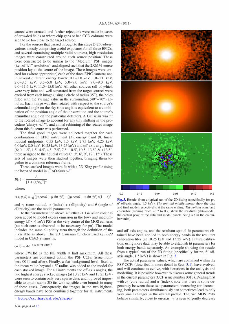
Fig. 3. Results from a typical run of the 2D fitting (specifically for pn,6′ off-axis angle, 1.5 keV). The top and middle panels show the dataand final model respectively, at the same scaling. The bottom panel andcolourbar (running from −0.2 to 0.2) show the residuals (data-model,the central peak of the data and model panels being ≈5 in the colour-bar units).

and off-axis angles, and the resultant spatial fit parameters ob-tained have been applied to both energy bands in the resultantcalibration files (at 10.25 keV and 13.25 keV). Future calibra-tion, using more data, may be able to establish fit parameters forboth energy bands separately. An example showing the resultsfrom a typical run of the 2D fitting (specifically for pn, 6′ off-axis angle, 1.5 keV) is shown in Fig. 3.

The actual parameter values, which are contained within thePSF CCFs (described in more detail in Sect. 3.1), have evolved,and will continue to evolve, with iterations in the analysis andmodelling. It is possible however to discuss some general trendsin the current parameters (CCF issue number 0013). Dealing firstwith r0 (core radius) and α (index), note that there is some de-generacy between these two parameters; increasing (or decreas-ing) both parameters simultaneously can sometimes lead to onlyvery small changes in the overall profile. The two MOS PSFsbehave similarly; close to on-axis, r0 is seen to gently decrease

A34, page 4 of 13

A. M. Read et al.: A new comprehensive 2D model of the PSFs of the XMM-Newton EPIC telescopes

Fig. 4. Schematic of the flat-topped triangular function used to parameterize the PSF spokes. The blue spoking function is constructed such that thered and the green areas exactly cancel out. The dashed line shows the unspoked function. The lengths 1.00, 0.165 (the half-width of the flat-top u)and 0.165 (the base to peak width v) are in units of half the inter-spoke distance, i.e., 11.25◦. The figure is not to scale.

with increasing energy, while α is seen to remain roughly con-stant with energy. The profile therefore is seen to get narrowerat higher energies, as expected, as only a fraction of the mir-ror shells − the smaller, inner shells − contribute to the higher-energy PSF. At larger off-axis angles, the MOS r0 and α valuesare seen to decrease with increasing energy, but more steeply,starting from larger low-energy values than is seen on-axis. Thepn PSF behaves slightly differently in that r0 decreases gentlywith increasing energy for all off-axis angles, but the averager0 value increases with off-axis angle (as expected, the PSF be-coming wider off-axis). The pn α is seen to remain roughly con-stant for almost all energies and off-axis angles, hence, in con-junction with the gently decreasing r0 values with energy, theprofile again gets narrower at higher energies. The ellipticitybehaves as one would expect and very similarly for each in-strument, getting larger with increasing off-axis angle, from≈0 on-axis to ≈0.6 far off-axis. Also the ellipticity is seen (moreprominently off-axis) to gently increase with increasing energyin each instrument. Finally, for the Gaussian component (whichexists only for the MOS cameras at E ≤ 6 keV), both the FWHMand the relative normalization for both MOS PSFs are seen to fallfrom 0 to 6 keV, for all off-axis angles (i.e., to match there beingno Gaussian at >6 keV).

2.2. The support structure features – The spokes

The radial spokes have been modelled with a flat-topped triangu-lar function (Fig. 4), chosen after consultations with mirror ex-perts (B. Aschenbach, priv. comm.; R. Willingale, priv. comm.).16 equally-spaced spokes have been included in the model. Thedistance between two consecutive peaks of the spoke functionis therefore 22.5◦. The shape of this function has been tuned insuch a way that it does not change the integral of the radial pro-file (i.e., the red and the green areas in Fig. 4 exactly cancel out).This filtering function is fixed in space with respect to the detec-tor, such that any axis of the DETX/Y (or RAWX/Y) coordinatesystem lies exactly between two spokes, and is only applied tothe elliptical envelope after the envelope has been rotated ac-cording to the azimuthal position of the source on the detector.

The current spoke dimensions have been obtained from mea-suring the azimuthal angles of the spoke troughs, peaks and flat-tops of a number of bright sources, including GX 339-4, usingthe full energy range (0.2−12 keV) and over a large radial range(20′′−100′′). The current dimensions are such that both the half-width of the flat-top (u), and the width from base to peak (v)equals 0.165 times half the width of the spoke-to-spoke distance(as indicated in Fig. 4). It can be shown that the height h of thespoke above the unspoked dashed line of Fig. 4 (if the spokedrops below the line by a depth of 1.0) is related to the half-width of the flat-top u and the base to peak width v via:

h =2

2u + v− 1.

The strength (intensity) of the primary spokes is set such that thespoked PSF is made up of (at most) 42% of an image formedfrom the flat-topped triangular function depicted in Fig. 4, andthe remainder is formed from an unspoked image. This is againbased on the spatial analysis of a number of bright sources. Theradial dependence of the intensity of the spoking is however notconstant (see below), and this intensity value (42%) is the maxi-mum value.

16 secondary spokes, observed in very bright sources(see Fig. 2), and situated half-way between the 16 main pri-mary spokes, are modelled with the same spoke function, ro-tated by 11.25◦ with respect to the main spoke system, and witha (maximum) intensity factor of 3.5%.

The relative strength of the spokes is not constant with radiusbut appears to vary. Owen & Ballet (2011) were able to charac-terize the radial dependence of the spokes of the MOS1, MOS2and pn PSFs to large radii (up to 2′) using bright, heavily piled-up sources, and using procedures developed to correct for theeffects of pile-up. They found that the radial dependence of thespokes of the two MOS cameras and the pn camera appeared tobe approximately the same. This is not surprising as the spokesand their radial dependencies are all due to the construction ofthe mirror modules, all of which were designed to be identi-cal. Furthermore the spiders were constructed out of Inconel,a material chosen for its thermal expansion, which is close to

A34, page 5 of 13

A&A 534, A34 (2011)

r=44"-88"

180 200 220 240Azimuth Angle (degrees)

0

50

100

150

Ct/P

ix

r=88"-132"

180 200 220 240Azimuth Angle (degrees)

0

10

20

30

40

Ct/P

ix

Fig. 5. A section of the azimuthal profile (black line) from GX 339-4(ObsID 0204730301) (MOS1, 0.2−12 keV) in annular extractions of(top) 44′′−88′′ and (bottom) 88′′−132′′. The current (CCF 0013) flat-topped triangular function for the primary spokes at maximum strength(i.e., at a radius of 110′′) is shown in blue (see text).

that of the electrolytic nickel of the mirrors (de Chambure et al.1999), thus keeping distortions to a minimum. This radial de-pendence has been modelled to match the Owen & Ballet (2011)on-spoke to off-spoke ratio results, and will be introduced intothe PSF CCFs (for issue numbers 0014 and after) as follows: foreach EPIC PSF, from the centre out to 10′′, there is no spoking.From 10′′to 110′′ the spoke strength increases linearly from zeroto the maximum (42%). From 110′′ to 180′′ the spoke strengthdecreases linearly from its maximum to zero, and there is nospoking beyond this radius.

Looking beyond the present model, when we compare in de-tail the azimuthal profile of good quality point source data withthe current (CCF 0013) model (see Fig. 5), there are a numberof points of interest: though there is significant statistical scatter,there may also be some true spoke-to-spoke variation. Further,it appears that there may be some variation of the spoke modelwidth parameters u and v with radius − the spokes appearing tobe narrower at larger radius. Interestingly it appears that thereis a significant difference in the radial dependence of the sec-ondary spoke strength, compared to that of the primary spokes −the secondary spokes falling off quicker (there also appears to besignificant secondary spoke-to-spoke variation). None of theseeffects (nor their energy-dependencies) are yet contained withinthe current PSF model, but they impinge upon e.g., the on-spoketo off-spoke Owen & Ballet (2011) results, and on their inter-pretation and modelling − note that the on-spoke to off-spokeratio is lower at smaller radius (44′′−88′′) than at larger ra-dius (88′′−132′′), partly because the secondary spokes are rela-tively stronger at smaller radius than at larger radius. It is hopedthat these issues can be revisited in future improvements in themodelling of the EPIC PSFs.

2.3. The support structure features – The large-scaleazimuthal modulation

The apparent triangular shape of the MOS2 PSF can be modelledby a spatial low frequency overall modulation of the PSF shape.

Table 1. Current parameters of the large-scale azimuthal multi-peakmodulation.

Cameras A N φ0

MOS1 13% 5 62◦MOS2 45% 3 50◦

Notes. The modulation M(φ) is modelled as a cosine function of theazimuthal angle φ, with A as the amplitude of the modulation, N beingthe number of peaks in the modulation in a full 360◦ revolution, andφ0 the azimuthal offset of the cosine function. φ and φ0 run clockwisefrom north for a source on the sky, for an observation Position Angle,PA = 0 (see text).

A pentagonal modulation is also present at a lower level in theMOS1 and also at a very low level in the pn PSF. These shapesare thought to be due to distortions and irregularities in certainsets of mirror shells within each of the telescopes – e.g., the outershells not being perfectly circular (de Chambure et al. 1999).It is not surprising therefore that these deformities are differentin the three EPIC PSFs.

This modulation M(φ) is modelled as a function of the az-imuthal angle φ, with a multi-peaked cosine function in the PSFsof the cameras:

M(φ) = A cos(Nφ − φ0)

where A is the amplitude of the modulation, N is the number ofpeaks in the modulation in a full 360◦ revolution, and φ0 is theazimuthal offset of the cosine function. The current parametersof this function are shown in Table 1.

The radial dependence of these large-scale azimuthal modu-lations is also seen not to be constant with radius, and the max-imum amplitude A is listed in Table 1. The dependence is onlyroughly similar to the radial dependence of the spokes, and thereare variations between the EPIC detectors – the pn pentagon forexample only appears to be visible over quite a narrow range inradius. This radial dependence of the large-scale azimuthal mod-ulations (and the entire pn large-scale azimuthal modulation) hasnot been fully calibrated yet, but will appear in a future issue ofthe PSF CCFs.

As a final step in the construction of the 2D PSF, a radially-dependent very light smoothing is applied. A smoothed imageof the PSF is constructed using a flat boxcar of halfwidth 1.65′′.The final PSF is then a sum of f times this smoothed image plus(1 − f ) times the original unsmoothed image, where f varieslinearly from 0 at the source center to unity at 8.8′′. Though thisdoes not currently directly match the more elliptical nature ofthe PSF at larger off-axis angle, this will be investigated further,and the smoothing effect is very small, has been applied merelyto de-pixelate the spoke structures at large radius, and does nothave any significant large-scale effects (e.g., on radial profiles).

2.4. Additional features

The new 2D PSF system has been designed to be modular,and it is quite straightforward to add in further complexities.There are a number of additional features to the EPIC PSFsthat will be added, it is intended, to future updates of the system(some may just require updates to the CCFs, others may requiresoftware and infrastructure changes). The radial dependenciesof the large-scale azimuthal modulations, as discussed above,is one. It is very probable, as the large-scale azimuthal modula-tions are due to deformations only in certain mirror shells, thatthere are energy-dependencies to this effect, and these will also

A34, page 6 of 13

A. M. Read et al.: A new comprehensive 2D model of the PSFs of the XMM-Newton EPIC telescopes

Fig. 6. The eight main steps in the formation of the full 2D PSF for a source in a given instrument, of a given energy and at a given off-axis andazimuthal angle: the King (beta2d) component [1] is constructed, then the Gaussian (gaus2d) core [2] is constructed, and these are added [3] inthe correct ratio (the CCF parameters in steps 1−3 are all functions of instrument, energy and off-axis angle). Then this is rotated [4] accordingto the azimuthal position of the source on the detector, and only then are the radially-dependent primary [5] and secondary [6] spoke structuresazimuthally filtered in, using a flat-topped triangular function. Finally, the large-scale azimuthal modulation (a function of EPIC instrument) isfiltered in [7], and the very light radially-dependent smoothing applied [8]. The example shown is for MOS2, at an energy of 1.5 keV, an off-axisangle of 9′, and a source azimuthal position of 30◦.

need to be incorporated. A further task is to include the effects ofthe dark lanes visible e.g., in Fig. 2, due to the electron deflector,mounted after the rear aperture of the mirrors and whose legsalign with those of the front-end spider. It should be possible,once calibrated, to insert this effect into the system, via a similarazimuthal filtering technique as for the spokes. Features due toOOTs have not been considered to be part of the PSF. Thoughinstrument-dependent, they are also mode-dependent, and interms of the source-detection software, they are modelled viaan alternative route (at least for the pn, where the OOT signal ismuch stronger). The OOT features here have, in a similar mannerto the azimuthal structures (the spokes, triangles etc.), been di-luted and smeared out via the stacking procedure prior to the en-velope fitting. Furthermore there is set within the PSF system thepossibility to allow for any azimuthal variations in the envelope2D King and Gaussian parameters. Currently the CCFs are setsuch that these parameters do not vary with source azimuth, butfuture calibration may require changes, e.g., to account for vari-ations due to the obscuring RGAs in the EPIC-MOS cameras.

3. Results: the 2D PSF in the XMM-Newton SAS

The new 2D PSF is contained within all XMM-Newton SAS PSFCCFs of the form XRTi_XPSF_nnnn.CCF, where nnnn, the is-sue number of the file, is 0011 or higher. The relevant parametersare contained within the ELLBETA_PARAMS extension.

A number of elements are used to describe the new 2D PSFin these CCFs, as summarized here:

– A (currently) azimuthal-angle-independent parameterizationof the elliptical PSF envelope as a function of instrument,energy, and off-axis angle. An additional Gaussian “core” is

added to the PSF envelope of the MOS cameras for low andmedium energies (E ≤ 6 keV) only.

– An azimuthal filter of the elliptical envelope, which de-scribes the effect of the spokes created by the spider support-ing the 58 co-axial mirrors of each telescope. Primary andsecondary spokes are included. The radial dependency of thestrength of these spokes is to be included in version 0013 ofthe CCFs. The parameters of this filtering are currently hard-coded into the CAL software, but will appear as FITS key-words in version 0013 of the CCFs. The filtering to accountfor the dark lanes will appear in future CCF releases.

– A further azimuthal dependency of the overall PSF enve-lope, which is responsible for the apparently triangular shapeof the MOS2 PSF. Lower level similar effects are presentin the PSFs of MOS1 and pn also. Currently, this correc-tion is applied to the PSFs of MOS1 and MOS2 only. Theparameters of this correction are currently hard-coded intothe CAL package, but will appear as FITS keywords in ver-sion 0013 of the CCFs. The pn correction and the radial de-pendencies for all three will be included in future releases ofthe CCFs.

A scheme of the different physical ingredients of the 2D PSF pa-rameterization and how they are combined to produce the fi-nal PSF is shown in Fig. 6. For a comparison with an actualEPIC off-axis source, Fig. 7 shows a very bright, ≈4′ off-axisangle MOS2 point source and the equivalent PSF model at asimilar off-axis and the appropriate source azimuthal position.

Once the 2D PSF was incorporated into both the CCF systemand the SAS, a next step was to compare it with the default PSFin terms of how well the SAS-constructed PSFs model the truesource structures. To this end, full SAS calibrated event list cre-ation, image formation and detection chain analysis (as per the

A34, page 7 of 13

A&A 534, A34 (2011)

Fig. 7. A very bright, slightly piled-up, ≈4′ off-axis angle MOS2 pointsource and the equivalent PSF model at a similar off-axis and the ap-propriate source azimuthal position.

standard pipeline) was performed on a large number of fieldscontaining bright, non-piled-up point sources, detected by EPIC,and (where available and where observing mode constraints al-lowed) in all three EPIC cameras. The detection chain anal-ysis was performed once using the default (MEDIUM) PSFand once using the 2D (ELLBETA) PSF. Next, taking greatcare to co-align each source image and each detection-chain-produced model PSF image, then for each source, both thesource and the model counts within each of 30 radial bins (each4′′ wide) and 32 azimuthal bins (each 11.25◦ wide, arranged tobe alternately fully on-spoke, then fully off-spoke) were com-puted. The co-alignment ensured that each azimuthal bin corre-sponded to the same azimuth on the PSF. This procedure wasperformed for 80 bright, non-piled up point sources, and the val-ues were stacked together, in several energy bands and off-axisangle groupings. All this analysis was performed using both the2D PSF and the default PSF.

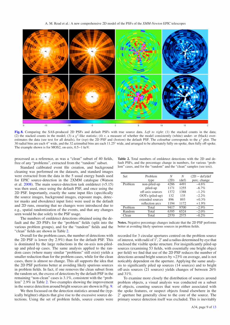
Figure 8 shows the results of this analysis, for the example ofMOS2, on-axis, 0.5−1 keV, arranged in the circular grid used of30 radial bins combined with 32 azimuthal bins. The top rowcorresponds to the 2D PSF, and shows (left to right): (1) thestacked counts in the data; (2) the stacked counts in the model;(3) a χ2-like statistic, calculated from the stacked data countsand stacked model counts as:

χ2 =±(stacked data − stacked model)2

stacked model,

and (4) r, a measure of whether the model consistently under- oroverestimates the data, and calculated as the sum of the individ-ual data – model “signs” via:

r =∑ data −model|data −model| ,

which ranges between+1 (white, always underestimates) and−1(black, always overestimates). The bottom row of Fig. 8 showsthe equivalent plots for the default PSF (and hence the twostacked data plots are identical). The colourbar (−20 to +20) cor-responds to the χ2 plot.

A number of conclusions can be drawn from this figure.Similar results are seen for MOS1 and pn, though some (e.g., todo with the large-scale azimuthal filtering) are harder to see.Very obvious is that the default PSF, due to its limitations dis-cussed in Sect. 1.1, performs very poorly with regard to thespokes; the on-spoke regions are very underestimated by thedefault model, and the off-spoke regions are overestimated.Secondly, the default PSF performs extremely badly in mod-elling the large-scale azimuthal features − here, the MOS2 tri-angle (note the very large triple-peaked discrepancies in the χ2

and r plots for the default PSF). The 2D PSF however, performs

very much better. Much less variation in χ2 and r is seen on- andoff-spoke. The plot does suggest though that the 2D PSF relativespoke strength may be too strong. The most up-to-date SAS andthe latest PSF CCF files that are available for this analysis (ver-sion 0012) however, do not yet include the radial dependencyof the spoke strength, and the future inclusion of this will act todecrease this effect, and improve further the 2D PSF modelling.The 2D PSF modelling of the MOS2 triangle is also very muchimproved over the default PSF. Further refinements to this com-ponent include the modelling of both its radial-dependence andits energy-dependence.

3.1. Description of the PSF CCF parameters

The FITS extension ELLBETA_PARAMS in the PSF CCFXRTi_XPSF_0011.CCF (and later) files contains the parametersdescribing the elliptical envelope and the Gaussian core. Thisextension contains four columns:

– ENERGY: the energy (in eV) to which the parameters refer;– THETA: the off-axis angle (in radians) to which the parame-

ters refer;– PHI: the azimuthal angle (in radians) to which the parame-

ters refer;– PARAMS: an array, containing the parameters of the

2D King (beta2d) plus Gaussian (gaus2d) function:– 1: the King core radius (r0), in arcseconds;– 2: the King power-law slope (α);– 3: the ellipticity (ε) (of both the King and the Gaussian

components);– 4: the Gaussian Full Width Half Maximum (FWHM), in

arcseconds;– 5: the normalisation ratio of the Gaussian peak to the

King peak (N).

4. Discussion: testing of the PSF

Though this paper is primarily concerned with a description ofthe new 2D PSF and its construction etc., it is very useful hereto discuss some of the testing, especially as regards the majorreason why the new 2D PSF was originally desirable – i.e., tosee if it could reduce the number of spurious sources detectedby the standard source-detection pipeline, where the relativelypoor description of the PSF can lead to large residuals in theconstructed data-minus-model images, leading in turn to the de-tection of spurious sources. Also of major interest are the as-trometry issues that have arisen as a consequence of these firsttests. These issues are discussed in the following sections.

4.1. Source-searching and spurious sources

A comparison of the performance of the new 2D PSF (“Ellbeta”)with that of the current existing default PSF (“Medium”) hasbeen performed, the primary objective being to establish whetherthe 2D PSF better suppresses the detection of spurious sources.The analysis first focussed on a set of 108 “problem” ob-servations containing examples of various types of situationswhere spurious sources had previously been found to be present.These were mainly chosen to be around non-piled-up brightsources, but there were also several fields chosen involvingbright piled-up sources, off-axis sources, extended sources, out-of-time (OOT) events from piled-up sources and single reflec-tion arcs. A separate “random” set of 83 observations was also

A34, page 8 of 13

A. M. Read et al.: A new comprehensive 2D model of the PSFs of the XMM-Newton EPIC telescopes

Fig. 8. Comparing the SAS-produced 2D PSFs and default PSFs with true source data. Left to right: (1) the stacked counts in the data;(2) the stacked counts in the model; (3) a χ2-like statistic; (4) r, a measure of whether the model consistently (white) under- or (black) over-estimates the data (see text for all details), for (top) the 2D PSF and (bottom) the default PSF. The colourbar corresponds to the χ2 plot. The30 radial bins are each 4′′ wide, and the 32 azimuthal bins are each 11.25◦ wide, and arranged to be alternately fully on-spoke, then fully off-spoke.The example shown is for MOS2, on-axis, 0.5−1 keV.

processed as a reference, as was a “clean” subset of 40 fields,free of any “problems”, extracted from the “random” subset.

Standard calibrated event file creation, and backgroundcleaning was performed on the datasets, and standard imageswere extracted from the data in the 5 usual energy bands usedfor EPIC source-detection in the 2XMM catalogue (Watsonet al. 2008). The main source-detection task emldetect (v5.15)was then used, once using the default PSF, and once using the2D PSF. Importantly, exactly the same input files (specificallythe source images, background images, exposure maps, detec-tor masks and eboxdetect input lists) were used in the defaultand 2D runs, ensuring that no changes were introduced due toe.g., spatial randomization of the events, and that any changesseen would be due solely to the PSF usage.

The numbers of emldetect detections obtained using the de-fault and the 2D PSFs for the “problem” fields (split into thevarious problem groups), and for the “random” fields and the“clean” fields are shown in Table 2.

Overall for the problem cases, the number of detections withthe 2D PSF is lower (by 2.9%) than for the default PSF. Thisis dominated by the large reductions in the on-axis non-piled-up and piled-up cases. The same analysis applied to the ran-dom cases (where many similar “problems” still exist) yields asmaller reduction than for the problem cases, while for the cleancases, there is almost no change. This all supports the idea thatthe 2D PSF performs better at avoiding likely spurious sourcesin problem fields. In fact, if one removes the clean subset fromthe random set, the excess of detections by the default PSF in theremaining “non-clean” cases is 3.1%, consistent with the “prob-lem” 2.9% in Table 2. Two examples showing the improvementin the source detection around bright sources are shown in Fig. 9.

We then focussed on the detection statistics around the (typ-ically brighter) objects that give rise to the excessive source de-tections. Using the set of problem fields, source counts were

Table 2. Total numbers of emldetect detections with the 2D and de-fault PSFs, and the percentage change in numbers, for various “prob-lem” cases, and for the “random” and the “clean” samples (see text).

Set Problem N N (2D − def)/deftype (2D) (def) perc. change

Problem non-piled-up 4286 4491 –4.6%piled-up 1171 1255 –6.7%

off-axis sources 1372 1388 –1.2%OOTs (piled-up) 132 135 –2.2%extended sources 896 893 +0.3%

reflection arcs 1194 1172 +1.9%Problem Total 9417 9700 –2.9%Random Total 6395 6524 –2.0%Clean Total 2570 2575 –0.2%

Notes. Negative percentage changes indicate that the 2D PSF performsbetter at avoiding likely spurious sources in problem fields.

recorded for 3 circular apertures centred on the problem sourceof interest, with radii of 1′, 2′ and a radius determined by eye thatenclosed the visible spoke structure. For insignificantly piled-upsources (examining 53 fields, with essentially one bright objectper field) we find that use of the 2D PSF reduces the number ofdetections around bright sources by ≈23% on average, and is notnoticably dependent on the aperture. Applying the same analy-sis to significantly piled up sources (14 sources) and to brightoff-axis sources (21 sources) yields changes of between 26%and 31%.

To examine more closely the distribution of sources aroundproblem objects, a visual analysis was conducted on a subsetof objects, counting sources that were either associated withthe spoke features, or suspect objects found elsewhere in the2′ aperture but generally close to the core of the source. Theprimary source detection itself was excluded. This is inevitably

A34, page 9 of 13

A&A 534, A34 (2011)

Fig. 9. Example output from a full all-EPIC source-detection analysis of ObsIDs 0107660201 (left) and 0302850201 (right). The blue circles showthe sources detected using the default PSF and the yellow circles show the sources detected using the 2D PSF. Many spurious sources previouslydetected by the default PSF in the spokes of the central bright source are now not detected by the 2D PSF.

Fig. 10. Distributions of the (2D-default) change in returned (left) RA and (right) Dec of detected sources using the 2D (Ellbeta) and default(Medium) PSF for a sample of 70 clean observations.

a subjective analysis and does not take account of the depen-dence on detection likelihood, but it provides a useful assess-ment of the impact of the 2D PSF. We find that for sourcesdetected on spokes, overall the 2D PSF finds >∼42% fewer de-tections than the default PSF (or >∼92% fewer if we consideronly detections on spokes that are not common to both PSFs).Likewise, for sources near the core of the primary source, the2D PSF yields at least 22% fewer detections, or >∼69% fewer ifwe exclude the common detections.

Thus, we conclude that use of the 2D PSF substantially re-duces the number of detections compared to the default PSF andthat this reduction is primarily due to fewer detections on thespokes and in the core regions of bright sources. These are pre-cisely the components of the PSF which are being better mod-elled by the 2D PSF. These model improvements suppress data-minus-model residuals that have hitherto given rise to spuriousdetections when using the default PSF.

4.2. Astrometry issues

A major outstanding concern in the comparison of the 2D PSFoutput with the default PSF output was that large and signifi-cant positional shifts are observed. Mean differences of ≈+0.8′′

in RA and ≈-0.8′′ in Dec (2D values minus default values) areobserved between the 2D and default PSF results on any largeset of observations. Figure 10 shows the distributions of the RAand Dec (2D-default) offsets for a sample of 70 observations(incorporating and extending on the clean sample of the previoussection).

It was not known whether this shift was due to the 2D PSF orto the default PSF (or to both). One source of confusion and pos-sible error is the fact that the default PSF (as described briefly inSect. 1.1) consists of a set of images of dimensions 512 × 512and pixel size 1.1′′ × 1.1′′. It was noted that the assumptionof where the centre of one of these images is, and the propa-gation, correctly or incorrectly, of this assumption through therelevant SAS subsystems (PSF and image generation, PSF ro-tation, source-searching etc.) could lead to possible errors. Thisthinking also indicated that the rotation of the PSF could be vi-tal in pinning down the root of the positional offset problem,and indeed, when the (2D-default) changes in RA and Dec areplotted against the source angle on the sky (Fig. 11), the +0.8′′and −0.8′′ offsets are resolved into not only offset, but sinusoidalvariations, indicating that (i) not only is there an offset problembetween the two PSFs; but (ii) the rotation of one (or both) ofthe PSFs contains an additional systematic sinusoidal error.

A34, page 10 of 13

A. M. Read et al.: A new comprehensive 2D model of the PSFs of the XMM-Newton EPIC telescopes

Fig. 11. (2D-default) offsets in (left) RA and (right) Dec of detected sources using the 2D (Ellbeta) and default (Medium) PSF plotted against thesource angle on the sky (anti-clockwise from north) for the sample of 70 clean observations as in Fig. 10.

In order to evaluate which of the PSFs is at fault, it is nec-essary to cross-correlate the X-ray positions obtained with thetwo PSFs with good-quality optical positions. Here we need tointroduce the boresight matrix. This was calculated from fieldsof many bright sources, e.g., OMC2/3 (Kirsch 2004), and subse-quently refined using 430 individual fields (Altieri 2004), cross-correlating the source X-ray positions (note, obtained using thedefault PSF) with their optical positions, and observing whichparticular offset in RA, Dec and position angle is seen to signif-icantly optimize the correlation. This final calibrated boresightmisalignment matrix has been applied to the determination ofthe X-ray sky position of every X-ray event in every calibratedevent file.

It is therefore the case that any translation or offset prob-lem that is due to the default (Medium) PSF is “corrected for”and calibrated out when implementing the current boresight mis-alignment matrix. As such, it is expected that the X-ray-opticalsource positional offsets for the default PSF will be centredaround zero, and indeed, this is seen to be the case. The 2D PSFoffsets are furthermore seen to be centred around the observed(Figs. 10 and 11) +0.8′′ and −0.8′′ offsets.

The clean samples of source detections (using both the2D PSF and the default PSF) were cross-correlated with theSloan Digital Sky Survey Quasar Catalog (Schneider et al. 2007)to a match radius of 10′′. In almost every case where there was amatch, it was the only match. We looked at the cross-correlationsusing the original (emldetect-obtained) X-ray positions and us-ing the X-ray positions obtained by the SAS program eposcorr.This program, eposcorr, performs a similar task to the boresightmisalignment matrix calculation in that, for each observation,it correlates the input (emldetect) source positions with the po-sitions from optical source catalogues, and checks whether thereare offsets in RA, Dec and position angle which optimize thecorrelation. If there are optimum offsets, these are then used tocorrect the input source positions which are then added as sepa-rate columns to the input X-ray source list.

When the (X − QSO) differences in RA and Dec betweenthe X-ray positions and the optical quasar positions are plottedagainst source angle on the sky for both the default PSF (Fig. 12)

and the 2D PSF (Fig. 13, both figures using the eposcorr-corrected output), several things are evident.

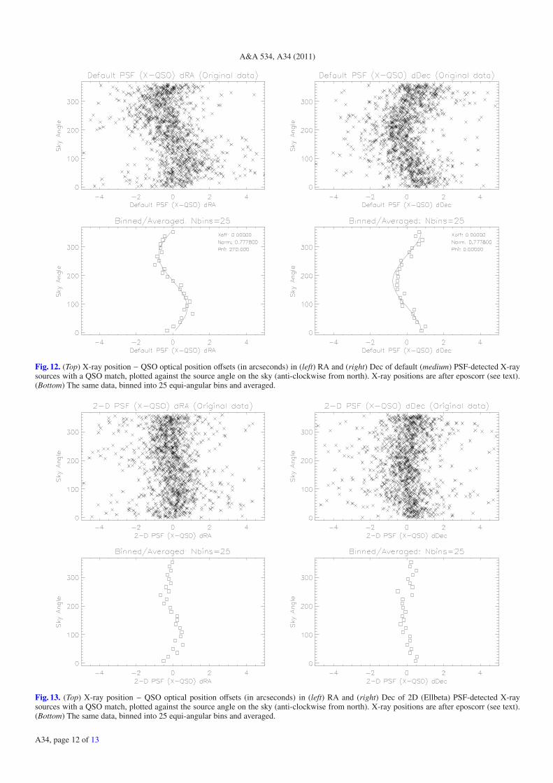
Firstly, regarding the offset problem, though the correspond-ing figures prior to eposcorr (not shown) do indeed show thedefault PSF distribution to be centred around zero offset, andthe 2D PSF distribution to be centred around the +0.8′′ and−0.8′′ offsets, the 2D PSF eposcorr output (Fig. 13) is centredaround zero − i.e., when it runs successfully, eposcorr is ableto correct the offset problem. Secondly, regarding the sinusoidalproblem, it is observed that it is for the default PSF case (Fig. 12)that the large sinusoidal variations are seen. For the 2D PSF(Fig. 13) the variations are very much smaller.

Looking in more detail, it was suggested earlier that the sinu-soidal problem could be related to the default PSF CCF images,and the assumptions regarding where the centres of these im-ages are, and how these assumptions are propagated through theentire PSF generation and source-searching system. This nowdoes appear to be the case, and added to the lower panels ofFig. 12 are simple calculated cosine curves of what one wouldexpect to see, given the simple offset of half the diagonal of asingle default PSF image pixel, rotated around the 360 degreesof the detector. The data is seen to match this simple model ex-tremely well. It is therefore undoubtedly the default PSF thatis the cause of the sinusoid effect, and this problem has existedfor the entirety of the XMM-Newton mission. The full positionalcapabilities of EPIC therefore have not been used to this date.The improvement here is such that, selecting the 67% of sourceswith a very good X-ray positional error (centroid error <1′′),the mean X-ray-QSO positional offset is reduced from 1.13′′(default) to 0.94′′ (2D), and the percentage of these sourceswith an X-ray-QSO positional offset less than 1′′ increases from52% (default) to 68% (2D). The percentage of cases where it isthe 2D PSF X-ray position that is the closest to the QSO positionis 70%.

Although the large sinusoids present in Fig. 12 have beenlargely removed in Fig. 13, they do not appear to have been com-pletely removed (and are at the 0.2′′−0.3′′ level). One shouldbear in mind that, if there is any inaccuracy at all present in thetrue positioning of the PSF centre, and where it is assumed to be

A34, page 11 of 13

A&A 534, A34 (2011)

Fig. 12. (Top) X-ray position − QSO optical position offsets (in arcseconds) in (left) RA and (right) Dec of default (medium) PSF-detected X-raysources with a QSO match, plotted against the source angle on the sky (anti-clockwise from north). X-ray positions are after eposcorr (see text).(Bottom) The same data, binned into 25 equi-angular bins and averaged.

Fig. 13. (Top) X-ray position − QSO optical position offsets (in arcseconds) in (left) RA and (right) Dec of 2D (Ellbeta) PSF-detected X-raysources with a QSO match, plotted against the source angle on the sky (anti-clockwise from north). X-ray positions are after eposcorr (see text).(Bottom) The same data, binned into 25 equi-angular bins and averaged.

A34, page 12 of 13

A. M. Read et al.: A new comprehensive 2D model of the PSFs of the XMM-Newton EPIC telescopes

in the PSF system, then a very similar sinusoidal variation willbe seen with source angle on the sky. The fact that some residualcurvature possibly exists in Fig. 13 may indicate that the situa-tion is not quite perfect, and there may still be a small residualmisalignment of the centering of the PSF system and the truePSF system.

At present, the 2D PSF only returns the optimum positionswhen eposcorr is run. Eposcorr only provides gross field shiftsand cannot correct for the residual sinusoidal effects. Also, theeposcorr task can not be run on every EPIC dataset, for instancein cases where there are very few (or very faint) X-ray sourcesin the field. In order for the full positional improvements of the2D PSF to be usable therefore, a revised boresight misalignmentmatrix first needs to be calibrated, tested and incorporated cor-rectly into the SAS (related SAS changes may also be required).This work, building on the above tests, is currently underway,and a future version of the SAS will include these improvementsin the positional accuracy of EPIC.

5. Conclusions

A new and fully comprehensive full-FoV 2D model of thePSFs of the three XMM-Newton EPIC telescopes has beenconstructed. This has been performed via the stacking, andbringing-together to a common reference frame, of a large num-ber of good quality, long-exposure, non piled-up, bright pointsources from different positions within the full FoV of eachEPIC detector. The resultant general PSF envelopes were thenazimuthally filtered to construct the primary and secondaryspoke structures (plus their radial dependencies) and the large-scale gross azimuthal PSF deformations that are observed. ThePSF model also includes an additional Gaussian core, whichaccounts for (at most) 2% of the enclosed energy flux in theEPIC-MOS cameras.

This PSF model is available for use within the XMM-NewtonSAS via the usage of CCFs XRTi_XPSF_0011.CCF and laterversions. The modular nature of the new PSF system allows forfurther corrections and refinements in the future.

Initial EPIC source-searching tests using this new PSF modelindicate that it performs significantly better with regard to the

major problem with the previous PSF; that of large numbers ofspurious source being detected in the wings of, or close to brightpoint sources. The numbers of these spurious sources detectedwith the new PSF model are greatly reduced.

These tests also uncovered a systematic error in the previousPSF system, such that returned source RA and Dec values wereseen to vary sinusoidally about the true position with source az-imuthal position angle on the sky. This error in the previousPSF system (the amplitude of the sinusoid being ≈0.8′′ in RAand in Dec) has existed since the beginning of the XMM-Newtonmission, and affects all the EPIC positional determinations per-formed thus far. Usage of the new PSF results in a much smalleramplitude sinusoid, and therefore an improved positional accu-racy. SAS changes, including a revised boresight misalignmentmatrix (presently under construction) are required to make fulluse of the improvements in the positional accuracy of EPIC in-troduced by the new PSF.

Acknowledgements. The XMM-Newton project is an ESA Science Mission withinstruments and contributions directly funded by ESA Member States and theUSA (NASA). We thank Matteo Guainazzi and Steve Sembay for careful read-ings of the paper, and the referee for useful comments which have improvedthe paper. A.M.R. and S.R.R. acknowledge the support of STFC/UKSA/ESAfunding.

References

Aschenbach, B., et al. 2000, ESA XMM-Newton Calibration Technical NoteCAL-TN-0005

Altieri, B. 2004, XMM-Newton CCF Release Note XMM-CCF-REL-168de Chambure, D., Lainé, R., van Katwijk, K., & Kletzkine, P. 1999, ESA Bull.,

100, 30den Herder, J. W., Brinkman, A. C., Kahn, S. M., et al. 2001, A&A, 365, L7Jansen, F., Lumb, D., Altieri, B., et al. 2001, A&A, 365, L1Kirsch, M. 2004, XMM-Newton CCF Release Note XMM-CCF-REL-156Owen, R., & Ballet, J. 2011, XMM-SSC Technical Note SSC-CEA-TN-1001Schneider, D. P., Hall, P. B., Richards, G. T., et al. 2007, AJ, 134, 102Strüder, L., Briel, U., Dennerl, K., et al. 2001, A&A, 365, L18Turner, M. J. L., Abbey, A., Arnaud, M., et al. 2001, A&A, 365, L27Watson, M., et al. 2008, A&A, 493, 339

A34, page 13 of 13