ABSTRACT

This paper presents a new common subexpression

elimination (CSE) algorithm for the realization of FIR filters

based on multiple constant multiplications (MCMs). This

algorithm shares the maximum number of partial terms

amongst the minimum signed digit (MSD)-represented

coefficients. The proposed algorithm modifies the iterated

matching (ITM) algorithm to share more partial terms in

MCMs and apply it to MSD-represented coefficients. These

modifications provide a significant logic and consequently

chip area savings. Employing the proposed algorithm yields

efficient realizations of FIR filters with fewer adders

compared to the conventional CSE algorithms.

Experimental results demonstrate that the proposed

algorithm can contribute up to a 22% reduction in the

complexity of FIR filters over some conventional CSE

algorithms. The proposed algorithm also addresses

challenges encountered in resource-constrained applications

that require banks of high-order filters such as in real-time

distributed optical fiber sensor applications.

Index Terms—Common subexpression elimination

(CSE), finite impulse response (FIR) filter, minimal signed

digit (MSD), multiple constant multiplications (MCMs)

1. INTRODUCTION

An FIR filter is a linear time invariant system governed

by a linear convolution of the input samples with the filter

coefficients, as shown in (1). In this equation, Ck stands for

the filter coefficients, and x[n] and y[n] denote the input and

output signals, respectively.

[ ] ∑ [ ]

The complexity of implementing FIR filters is mainly

dominated by product operations between filter coefficients

and input samples as reflected in the transposed structure of

the FIR filter in Fig. 1.

In recent years, there has been an increasing demand for

efficient implementations of FIR filters driven by high

accuracy and low power consumption requirements as well

as the flexibility of their implementation on hardware

platforms such as field programmable gate arrays (FPGAs)

or application specific integrated circuits (ASICs).

In applications such as distributed optical fiber sensors

[1], the use of higher order filters with long bit-width

coefficients is necessary, as the specification of filters

should be exactly met. An efficient implementation of

higher order filters with long bit-width coefficients is a

major challenge since there are always tradeoffs concerning

accuracy, power consumption, and speed in hardware

implementations. Therefore, the realization of FIR filters

with a reasonable tradeoff is demanding.

As shown in the transposed structure of the FIR filter, the

same input sample is multiplied by a set of coefficients at

each time. This kind of operation is known as multiple

constant multiplications (MCMs) and provides the

opportunity to realize FIR filters with a less amount of

computational resources.

The realization of MCMs is closely related to the

substitution of constant multiplications by shift and addition

operations. The substitution of multipliers with adders and

shift-registers enables significant savings in hardware

platform resources as they are more cost-efficient than

multipliers. It also enables the utilization of algorithms for

the detection of redundancies among constants and sharing

of partial terms.

In general, algorithms used for realizations of MCMs are

categorized into two approaches: graph-dependence (GD)

and common subexpression elimination (CSE).

The GD approach relies on the graph theory to synthesize

the coefficients of a filter with a number of primitive

Mohsen Amiri Farahani, Student Member, IEEE, Eduardo Castillo-Guerra, Bruce G. Colpitts, Senior Members, IEEE

Department of Electrical and Computer engineering, University of New Brunswick, Canada

A New Algorithm for Realization of FIR Filters

Using Multiple Constant Multiplications

Z -1 +

× CN-1 × CN-2

Z -1 +

× CN-3

Z -1 +

× C1 × C0

Z -1

Y[n]

X[n]

+

Fig. 1. Transposed structure of the FIR filter.

arithmetic operations [2]. It models inner products of input

samples by nodes of the graph and the shift operations by

edges of the graph.

Several GD algorithms such as Bull Horrock’s modified

(BHM) [3] and reduced adder graph (RAG) [4] have been

reported in the literature. Recently, significantly more

efficient GD-based algorithms were introduced in [5], [6].

The authors in [5] used a new graph structure to code the set

of coefficients based on their probability and conditional

probability of occurrence. Voronenko and Püschel in [6]

presented an optimal GD-based algorithm, which

extensively explores possible partial products (intermediate

vertices) among constants.

The CSE approach is a subset of the general adder graph

theory. They encounter the MCM problem with respect to

the numerical representation of constants.

Hartley algorithm is one of the first reported CSE

algorithms [7]. It searches through canonical signed digit

(CSD)-represented coefficients to find several common

subexpressions that can be conveniently reduced to a single

instance. The efficient numerical representations such as

CSD or minimal signed digit (MSD) are more demanding as

they represent numbers with fewer nonzero bits than normal

binary representation [8].

The iterative matching (ITM) algorithm in [9] is another

basic algorithm of CSE. It finds the maximum coincidences

between pairs of constants based on the most common

pattern and then eliminates a number of parallel adders

between them. In [10], some modifications were applied to

the ITM algorithm to maximize the sharing of partial terms

amongst constants having binary or CSD representations.

Same as GD-based algorithms, the CSE algorithms have

enabled a reduction in area and power consumption and an

increase in the throughput when they are employed to

implement FIR filters. In [11], the logic depth of filters was

reduced by using each common subexpression only one

time.

To share a maximum number of adders amongst the

constants and to realize MCMs with a shorter logic depth,

we present a new CSE algorithm by modifying the ITM

algorithm presented in [9]. The proposed algorithm searches

inside MSD-represented constants to find the best match,

and then uses the pattern corresponding to the best match to

do further optimization steps.

The remainder of the paper is organized into several

sections. In Section 2, we present the limitations of the ITM

algorithm. Section 3 introduces the proposed algorithm. The

results of comparison between the proposed algorithm and

some conventional algorithms are presented in Section 4.

Finally, the conclusion along with the scope of future work

is presented in the last section.

2. LIMITATIONS OF ITM ALGORITHM

In this section, we analyze the ITM algorithm [9] and

exlpain its main limitation: sharing the maximum number of

partial terms in realization of MCMs. For simplicity and

clarity, a basic example (Example 1) consisting of a set of

three constants, H = {c0, c1, c2}, is used. Table I shows the

set of constants and their CSD representation.

Table I

The set of constants of Example 1.

c0 583 0 1 0 0 1 0 0 1 0 01

c1 143 0 0 0 1 0 0 1 0 0 01

c2 -1145 10 010 0 0 1 0 01

The ITM algorithm selects partial terms based on the

most common patterns amongst the constants. The common

patterns are chosen in advance based on the bitwise matches

amongst constants.

The ITM algorithm presented in [9] can be briefly

analyzed in three steps as follows:

1- The calculation of the current (immediate) saving in

adders. The immediate saving is the number of

adders that can be saved based on the nonzero

bitwise matches amongst pairs of constants. For

example, there are two nonzero bitwise matches

between c0 and c2, that make the immediate saving

of this pair equal to one. Table II shows the

immediate savings for the set of Example 1.

Table II

Immediate savings for the set of Example 1.

c0 c1 c2

c0 - 0 1

c1 0 - 0

c2 1 0 -

2- The calculation of the later (future) saving in adders.

The future saving is the number of adders that can

be saved at the next iteration of the algorithm. For

the set of Example 1, there is no future saving as

there is no match amongst constants in the next

iteration of the algorithm.

3- The selection of the best match using the immediate

and future savings. Based on Table II, the best

match is between c0 and c2 and the pattern

corresponding to the best match (the matched digit)

is “1001 ”.

4- Updating the set of constants. The algorithm

updates the set of constants by adding a constant

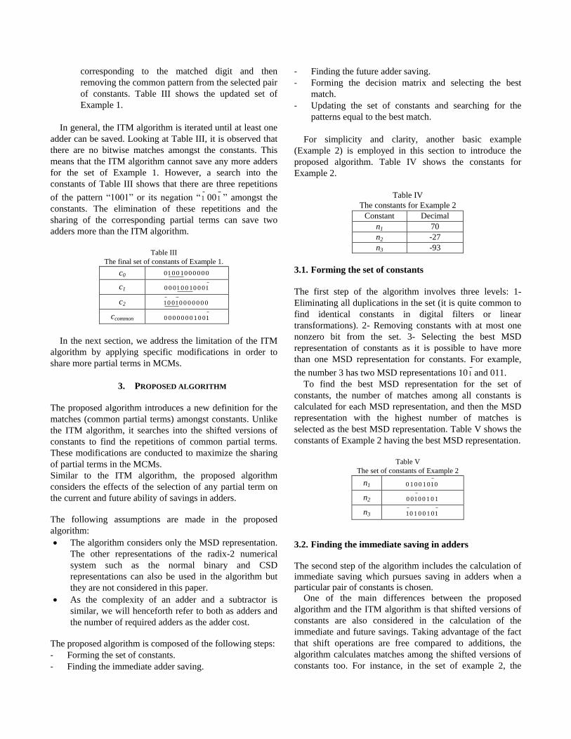
corresponding to the matched digit and then

removing the common pattern from the selected pair

of constants. Table III shows the updated set of

Example 1.

In general, the ITM algorithm is iterated until at least one

adder can be saved. Looking at Table III, it is observed that

there are no bitwise matches amongst the constants. This

means that the ITM algorithm cannot save any more adders

for the set of Example 1. However, a search into the

constants of Table III shows that there are three repetitions

of the pattern “1001” or its negation “1 001 ” amongst the

constants. The elimination of these repetitions and the

sharing of the corresponding partial terms can save two

adders more than the ITM algorithm.

Table III

The final set of constants of Example 1.

c0 01001000000

c1 0 0 01 0 0 10 0 01

c2 10 010 0 0 0 0 0 0

ccommon 0 0 0 0 0 0 0 1 0 01

In the next section, we address the limitation of the ITM

algorithm by applying specific modifications in order to

share more partial terms in MCMs.

3. PROPOSED ALGORITHM

The proposed algorithm introduces a new definition for the

matches (common partial terms) amongst constants. Unlike

the ITM algorithm, it searches into the shifted versions of

constants to find the repetitions of common partial terms.

These modifications are conducted to maximize the sharing

of partial terms in the MCMs.

Similar to the ITM algorithm, the proposed algorithm

considers the effects of the selection of any partial term on

the current and future ability of savings in adders.

The following assumptions are made in the proposed

algorithm:

The algorithm considers only the MSD representation.

The other representations of the radix-2 numerical

system such as the normal binary and CSD

representations can also be used in the algorithm but

they are not considered in this paper.

As the complexity of an adder and a subtractor is

similar, we will henceforth refer to both as adders and

the number of required adders as the adder cost.

The proposed algorithm is composed of the following steps:

- Forming the set of constants.

- Finding the immediate adder saving.

- Finding the future adder saving.

- Forming the decision matrix and selecting the best

match.

- Updating the set of constants and searching for the

patterns equal to the best match.

For simplicity and clarity, another basic example

(Example 2) is employed in this section to introduce the

proposed algorithm. Table IV shows the constants for

Example 2.

Table IV

The constants for Example 2

Constant Decimal

n1 70

n2 -27

n3 -93

3.1. Forming the set of constants

The first step of the algorithm involves three levels: 1-

Eliminating all duplications in the set (it is quite common to

find identical constants in digital filters or linear

transformations). 2- Removing constants with at most one

nonzero bit from the set. 3- Selecting the best MSD

representation of constants as it is possible to have more

than one MSD representation for constants. For example,

the number 3 has two MSD representations 101 and 011.

To find the best MSD representation for the set of

constants, the number of matches among all constants is

calculated for each MSD representation, and then the MSD

representation with the highest number of matches is

selected as the best MSD representation. Table V shows the

constants of Example 2 having the best MSD representation.

Table V

The set of constants of Example 2

n1 0 1 0 0 1 010

n2 0 010 0 1 0 1

n3 10 1 0 0 1 01

3.2. Finding the immediate saving in adders

The second step of the algorithm includes the calculation of

immediate saving which pursues saving in adders when a

particular pair of constants is chosen.

One of the main differences between the proposed

algorithm and the ITM algorithm is that shifted versions of

constants are also considered in the calculation of the

immediate and future savings. Taking advantage of the fact

that shift operations are free compared to additions, the

algorithm calculates matches among the shifted versions of

constants too. For instance, in the set of example 2, the

constant n1 can be shifted one digit to the left or right and

then be compared with other constants to find common

patterns between them.

In addition to the consideration of shifted versions of

constants, in this work (unlike the ITM algorithm), the

definition of matches is also extended to: 1- The bitwise

match between two constants (what has been done in the

ITM algorithm) and 2- The bitwise match between one

constant and the negation of the other one (called negated

match). For example, there is a negated match between n1 =

“ 0 1 0 0 1 010 ” and n2 = “ 0 010 0 1 0 1 ” with the common pattern

“100001 ”. This extension in the definition of matches in the

proposed algorithm enables the sharing of more common

partial terms amongst the constants.

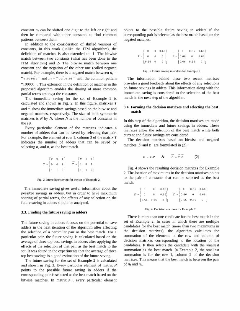
The immediate saving for the set of Example 2 is

calculated and shown in Fig. 2. In this figure, matrixes T

and T show the immediate savings based on the bitwise and

negated matches, respectively. The size of both symmetric

matrixes is N by N, where N is the number of constants in

the set.

Every particular element of the matrixes indicates a

number of adders that can be saved by selecting that pair.

For example, the element at row 1, column 3 of the matrix T indicates the number of adders that can be saved by

selecting n1 and n3 as the best match.

The immediate saving gives useful information about the

possible savings in adders, but in order to have maximum

sharing of partial terms, the effects of any selection on the

future saving in adders should be analyzed.

3.3. Finding the future saving in adders

The future saving in adders focuses on the potential to save

adders in the next iteration of the algorithm after affecting

the selection of a particular pair as the best match. For a

particular pair, the future saving is calculated based on the

average of three top best savings in adders after applying the

effects of the selection of that pair as the best match to the

set. It was found in the experiments that the average of three

top best savings is a good estimation of the future saving.

The future saving for the set of Example 2 is calculated

and shown in Fig. 3. Every particular element of matrix P

points to the possible future saving in adders if the

corresponding pair is selected as the best match based on the

bitwise matches. In matrix P , every particular element

points to the possible future saving in adders if the

corresponding pair is selected as the best match based on the

negated matches.

The information behind these two recent matrixes

provides a good feedback about the effects of any selections

on future savings in adders. This information along with the

immediate saving is considered to the selection of the best

match in the next step of the algorithm.

3.4. Forming the decision matrixes and selecting the best

match

In this step of the algorithm, the decision matrixes are made

using the immediate and future savings in adders. These

matrixes allow the selection of the best match while both

current and future savings are considered.

The decision matrixes based on bitwise and negated

matches, D and D are formulated in (2).

Fig. 4 shows the resulting decision matrixes for Example

2. The location of maximums in the decision matrixes points

to the pair of constants that can be selected as the best

match.

There is more than one candidate for the best match in the

set of Example 2. In cases in which there are multiple

candidates for the best match (more than two maximums in

the decision matrixes), the algorithm calculates the

summation of the elements in the row and column of

decision matrixes corresponding to the location of the

candidates. It then selects the candidate with the smallest

summation as the best match. In Example 2, the smallest

summation is for the row 1, column 2 of the decision

matrixes. This means that the best match is between the pair

of n1 and n2.

0 0 1

0 0 1

1 1 0

T

0 1 1

1 0 1

1 1 0

T

Fig. 2. Immediate saving for the set of Example 2.

0 0 0 .6 6

0 0 0

0 .6 6 0 0

P

0 0 .6 6 0 .6 6

0 .6 6 0 0 .6 6

0 .6 6 0 .6 6 0

P

Fig. 3. Future saving in adders for Example 2.

.D T P & .D T P (2)

0 0 0 .6 6

0 0 0 .6 6

0 .6 6 0 .6 6 0

D

0 0 .6 6 0 .6 6

0 .6 6 0 0 .6 6

0 .6 6 0 .6 6 0

D

Fig. 4. Decision matrixes for Example 2.

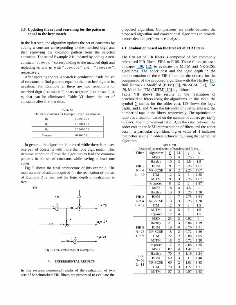
3.5. Updating the set and searching for the patterns

equal to the best match

In the last step, the algorithm updates the set of constants by

adding a constant corresponding to the matched digit and

then removing the common pattern from the selected

constants. The set of Example 2 is updated by adding a new

constant “ 0 0 1 0 0 0 01 ” corresponding to the matched digit and

replacing n1 and n2 with “ 0 0 0 0 1 0 0 0 ” and “ 0 0 0 0 0 1 0 0 ”,

respectively.

After updating the set, a search is conducted inside the set

of constants to find patterns equal to the matched digit or its

negation. For Example 2, there are two repetitions of

matched digit (“ 0 0 1 0 0 0 01 ”) or its negation (“ 0 010 0 0 0 1 ”) in

n3 that can be eliminated. Table VI shows the set of

constants after first iteration.

Table VI

The set of constants for Example 2 after first iteration.

n1 0 0 0 0 1 0 0 0

n2 0 0 0 0 0 1 0 0

n3 0 0 0 0 0 0 0 0

ncommon 0 010 0 0 0 1

In general, the algorithm is iterated while there is at least

one pair of constants with more than one digit match. This

iteration condition allows the algorithm to find the common

patterns in the set of constants while saving at least one

adder.

Fig. 5 shows the final architecture of this example. The

total number of adders required for the realization of the set

of Example 2 is four and the logic depth of realization is

two.

4. EXPERIMENTAL RESULTS

In this section, numerical results of the realization of two

sets of benchmarked FIR filters are presented to evaluate the

proposed algorithm. Comparisons are made between the

proposed algorithm and conventional algorithms to provide

a more detailed performance analysis.

4.1. Evaluation based on the first set of FIR filters

The first set of FIR filters is composed of five commonly

referenced FIR filters, FIR1 to FIR5. Those filters are used

in paper [10], [12] to evaluate the MITM and NR-SCSE

algorithms. The adder cost and the logic depth in the

implementation of these FIR filters are the criteria for the

comparison of the proposed algorithm with the Hartley [7],

Bull Horrock’s Modified (BHM) [3], NR-SCSE [12], ITM

[9], Modified ITM (MITM) [10] algorithms.

Table VII shows the results of the realization of

benchmarked filters using the algorithms. In this table, the

symbol ∑ stands for the adder cost, LD shows the logic

depth, and L and N are the bit-width of coefficients and the

number of taps in the filters, respectively. The optimization

ratio γ is a function based on the number of adders per tap (γ

= ∑/N). The improvement ratio, Λ, is the ratio between the

adder cost in the MSD representation of filters and the adder

cost in a particular algorithm. higher value of Λ indicates

that better saving in adders achieved by using that particular

algorithm. TABLE VII

Results of the realization of benchmarked filters.

Filter Algorithm ∑ LD γ Λ

FIR 1

N = 4

L = 10

MSD 15 4 3.75 1

Hartley 10 3 2.5 1.5

BHM 9 7 2.25 1.67

NR-SCSE 9 2 2.25 1.67

ITM 12 3 3 1.25

MITM 9 3 2.25 1.67

Proposed 8 2 2 1.87

FIR 2

N = 4

L = 12

MSD 18 4 4.5 1

Hartley 13 3 3.25 1.38

BHM 11 7 2.75 1.64

NR-SCSE 13 3 3.25 1.38

ITM 12 5 3 1.5

MITM 12 5 3 1.5

Proposed 12 4 3 1.5

FIR 3

N =25

L = 9

MSD 23 2 0.92 1

Hartley 21 3 0.84 1.19

BHM 19 6 0.76 1.31

NR-SCSE 18 2 0.72 1.39

ITM 22 2 0.88 1.05

MITM 18 2 0.72 1.28

Proposed 17 2 0.68 1.35

FIR4

N= 59

L= 14

MSD 87 4 1.47 1

Hartley 70 4 1.19 1.24

BHM 59 3 1 1.48

NR-SCSE 60 2 1.01 1.45

ITM 73 3 1.22 1.21

MITM 57 3 0.97 1.53

Fig. 5. Final architecture of Example 2.

Proposed 57 3 0.97 1.53

FIR5

N= 60

L= 14

MSD 114 6 1.9 1

Hartley 85 4 1.42 1.35

BHM 61 8 1.02 1.86

NR-SCSE 58 3 0.97 1.96

ITM 66 4 1.10 1.72

MITM 57 3 0.95 2.00

Proposed 56 3 0.93 2.04

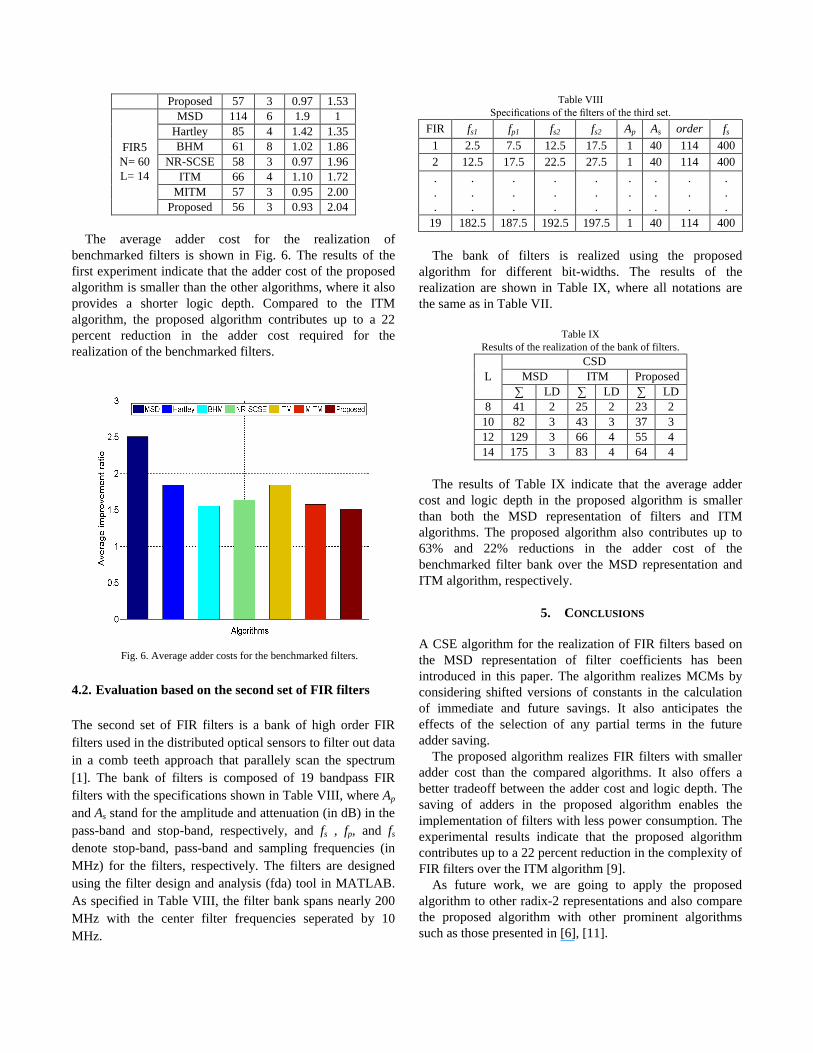
The average adder cost for the realization of

benchmarked filters is shown in Fig. 6. The results of the

first experiment indicate that the adder cost of the proposed

algorithm is smaller than the other algorithms, where it also

provides a shorter logic depth. Compared to the ITM

algorithm, the proposed algorithm contributes up to a 22

percent reduction in the adder cost required for the

realization of the benchmarked filters.

4.2. Evaluation based on the second set of FIR filters

The second set of FIR filters is a bank of high order FIR

filters used in the distributed optical sensors to filter out data

in a comb teeth approach that parallely scan the spectrum

[1]. The bank of filters is composed of 19 bandpass FIR

filters with the specifications shown in Table VIII, where Ap

and As stand for the amplitude and attenuation (in dB) in the

pass-band and stop-band, respectively, and fs , fp, and fs

denote stop-band, pass-band and sampling frequencies (in

MHz) for the filters, respectively. The filters are designed

using the filter design and analysis (fda) tool in MATLAB.

As specified in Table VIII, the filter bank spans nearly 200

MHz with the center filter frequencies seperated by 10

MHz.

Table VIII

Specifications of the filters of the third set.

FIR fs1 fp1 fs2 fs2 Ap As order fs

1 2.5 7.5 12.5 17.5 1 40 114 400

2 12.5 17.5 22.5 27.5 1 40 114 400

.

.

.

.

.

.

.

.

.

.

.

.

.

.

.

.

.

.

.

.

.

.

.

.

.

.

.

19 182.5 187.5 192.5 197.5 1 40 114 400

The bank of filters is realized using the proposed

algorithm for different bit-widths. The results of the

realization are shown in Table IX, where all notations are

the same as in Table VII.

Table IX

Results of the realization of the bank of filters.

L

CSD

MSD ITM Proposed

∑ LD ∑ LD ∑ LD

8 41 2 25 2 23 2

10 82 3 43 3 37 3

12 129 3 66 4 55 4

14 175 3 83 4 64 4

The results of Table IX indicate that the average adder

cost and logic depth in the proposed algorithm is smaller

than both the MSD representation of filters and ITM

algorithms. The proposed algorithm also contributes up to

63% and 22% reductions in the adder cost of the

benchmarked filter bank over the MSD representation and

ITM algorithm, respectively.

5. CONCLUSIONS

A CSE algorithm for the realization of FIR filters based on

the MSD representation of filter coefficients has been

introduced in this paper. The algorithm realizes MCMs by

considering shifted versions of constants in the calculation

of immediate and future savings. It also anticipates the

effects of the selection of any partial terms in the future

adder saving.

The proposed algorithm realizes FIR filters with smaller

adder cost than the compared algorithms. It also offers a

better tradeoff between the adder cost and logic depth. The

saving of adders in the proposed algorithm enables the

implementation of filters with less power consumption. The

experimental results indicate that the proposed algorithm

contributes up to a 22 percent reduction in the complexity of

FIR filters over the ITM algorithm [9].

As future work, we are going to apply the proposed

algorithm to other radix-2 representations and also compare

the proposed algorithm with other prominent algorithms

such as those presented in [6], [11].

Fig. 6. Average adder costs for the benchmarked filters.

REFERENCES

[1] P. Chaube et all., “Distributed fiber-optic sensor for dynamic

strain measurement,” IEEE Sensors Journal, vol. 8, no. 7,

July 2008.

[2] A. Dempster and M. D. Macleod, “Constant integer

multiplication using minimum adders,” Proc. Inst. Elec. Eng.

Circuits and Systems, vol. 141, no. 5, pp. 407–413, 1994.

[3] D. R. Bull and D. H. Horrocks, “Primitive operator digital

filter,” Proc. Inst. Elec. Eng. Circuits, Devices and Systems,

vol. 138, pt. G, pp. 401–412, 1991.

[4] A. Dempster and M. D. Macleod, “Use of minimum-adder

multiplier blocks in FIR digital filters,” IEEE Trans. Circuits

Syst. II, vol. 42, pp. 569–577, 1995.

[5] C. H. Chang, J. Chen, and A. P. Vinod, “Information theoretic

approach to complexity reduction of FIR filter design,” IEEE

Trans. Circuits Syst. I, Reg. Papers, vol. 55, no. 8, pp. 2310-

2321, Sep. 2008.

[6] Y. Voronenko and M. Puschel, “Multiplierless multiple

constant multiplication,” ACM Trans. Algorithms, vol. 3, no.

2, May 2007.

[7] R. Hartley, “Optimization of canonical signed digit

multipliers for filter design,” IEEE Int. Symp. Circuits Syst.,

Singapore, pp. 1992–1995, 1991.

[8] M. D. Macleod and A. G. Dempster, “Multiplierless FIR filter

design algorithms,” IEEE Signal Process. Lett., vol. 12, no. 3,

pp. 186–189, 2005.

[9] M. Potkonjak et al., “Multiple constant multiplication:

Efficient and versatile framework and algorithms for

exploring common subexpression elimination,” IEEE Trans.

Comput. Aid. Des., vol. 15, no. 2, pp. 151–165, 1996.

[10] M. A. Farahani, E. C. Guerra, and B. G. Colpitts, “Efficient

implementation of FIR filters based on a novel common

subexpression elimination algorithm,” CCECE’10, 2010.

[11] L. Aksoy et al., “Exact and approximate algorithms for the

optimization of area and delay in multiple constant

multiplications,” IEEE Trans. Comput. Aid. Des. Integr.

Circuits Syst., vol. 27, no. 6, pp. 1013-1026, 2008.

[12] M. M. Peiro, E. I. Boemo, and L. Wanhammar, “Design of

high-speed multiplierless filters using a nonrecursive signed

common subexpression algorithm,” IEEE Trans. Circuits

Syst. II, Analog Digit. Signal Process. vol. 49, no. 3, pp. 196–

203, 2002.