A Micro-Econometric Model of a Short Run Cost Function with Unobserved Heterogeneity*

David Prentice School of Business

La Trobe University, Bundoora, VIC, 3083. March 2000

Phone: 0394791482 Fax: 0394791654

email: d.prentice@latrobe.edu.au

* This paper is a revised version of Chapter Three of my Ph.D. dissertation written at Yale University. I would like to thank my supervisors Steven Berry, Moshe Buchinsky and Joel Waldfogel for their advice and support. This paper has also benefited greatly from comments at various stages by Tom Crossley, Iain Fraser, Tue G∅rgens, John Kennedy, Lisa Magnani, Gylfi Magnusson, Ariel Pakes and Rabee Tourky. Helpful comments were also received from participants in seminars at La Trobe University, Monash University, University of Melbourne, UNSW, University of Sydney, RSSS-ANU and Yale University. I would also like to thank Tony Salvage for assistance with the diagrams. I am most appreciative to Curtis Betts and the FW Dodge Co. for the use of the construction data. All errors remain my own responsibility.

Summary

Unobserved plant level heterogeneity and discrete production processes can

produce problems for estimation. A structural model of discrete production decisions

by heterogeneous plants is constructed and, as a case study, estimated for the U.S.

Portland cement industry. A new estimator is proposed to handle the discrete

production process – for which the ordered probit is a special case. Data on firm

survival and exit are used to adjust all input requirement coefficients for unobserved

heterogeneity. The structural model is successfully estimated. Differences between

many estimated coefficients and independent estimates from external sources are

statistically insignificant.

1. Introduction

The short run cost function plays a key role in estimating market power or

predicting input and output decisions. Estimation in the new empirical industrial

organization, and elsewhere, typically proceeds by assuming that the common short

run marginal cost function is both convex and continuous in either all outputs or, as

with hedonic cost functions, in product characteristics. However, recent work

suggests models based on these assumptions are not always appropriate for empirical

work. One set of papers demonstrates productivity and size varies substantially across

plants within industries resulting in divergent responses to common shocks (e.g.,

Davis and Haltiwanger (1992)). Furthermore, not controlling for this heterogeneity

results in biased estimation (Olley and Pakes (1996)). A second set of papers presents

evidence that production is sometimes better characterised as a discrete rather than a

continuous choice and that cost functions may be non-convex (e.g., Bresnahan and

Ramey (1994)). If the cost function is severely misspecified then other results could

be compromised.

In this paper, I specify a structural model of a plant short run marginal cost

function in an industry featuring both plant level heterogeneity and discrete

production decisions across multiple units. A new estimator is proposed to handle the

discrete production decisions. Furthermore, the model is extended to deal with

incomplete information about plant output and unobserved cost heterogeneity. In

particular, plant exit and survival data is used to control for cost differences across

operating plants. The structural model is estimated with a new unusually detailed

dataset on the U.S. Portland cement industry. Estimates of some parameters of the

cost function are found to not differ significantly from independent estimates obtained

from trade journals and input consumption data.

The model estimated in this paper significantly improves on earlier work in

three ways. First, the discrete production decision rule for multiple units is estimated

more directly and completely than in Bertin, Bresnahan and Raff (1996). Second,

input requirement coefficients are adjusted directly for unobservable plant level

1

heterogeneity unlike in Olley and Pakes (1996) and Dionne et al (1998) where the

effects of unobservable heterogeneity are introduced a more limited way. Finally, the

methodology and model improves on earlier work by being implementable with

datasets typically available to firms or consultants rather than specialized datasets

such as census unit record data. Thus the model and technique are more broadly

applicable. So, before applying standard techniques in industry analysis, the

importance of plant heterogeneity and discrete production decisions should be

checked. Where these conditions are important, the techniques presented in this paper

can be applied.

The structural model is developed explicity for the U.S. Portland cement

industry. This is done, in part, for clarity. It is important to stress, though, that the

model and methodology can be applied to a broad set of industries which feature

discrete production processes and multiple production units or plants, including steel

and electricity generation. However, the cement industry requires less simplifying

assumptions than typical when econometrically analyzing a manufacturing industry

for several reasons. First, cement is essentially homogeneous. Second, it is produced

by a relatively simple fixed proportions production process. Third, at least some of the

most important sources of plant level heterogeneity are observable and they can be

systematically included in both the modelling of the production decision and in the

estimation of the short run cost function. Finally, the discrete production choice is a

direct implication of the combination of the technology and the nature of competition

in the industry.

In the next section, the short run cost function for a plant with multiple

heterogeneous production units is derived yielding two discrete decision rules for

production and retirement. The data are then introduced in Section 3. In Section 4, the

model and data are reconciled and integrated producing a structural model for

estimation, with a new estimator, of the short run cost function. Section 5 presents the

results and in Section 6 some conclusions are presented.

2

2. The Short Run Cost Function

Cement is the powder that is mixed with sand, aggregates and water to

produce concrete. Most cement is a standard grey Portland cement effectively

homogeneous across sellers. The primary use of concrete is in construction so cement

consumption varies directly with construction activity. Demand is substantially

separable across years because construction, in most parts of the United States, is

concentrated in the summer and fall.

In subsequent subsections, the short run cost function for a cement plant is

presented. Though such a function could easily be applied to similar industries. Then

it is argued that the plant can be modelled as a price taker. This section concludes

with two decision rules for the cement plant for production and retiring capital. The

first decision rule provides the foundation for estimating the short run marginal cost

function. The second rule is used to control for unobserved heterogeneity in

productivity.

2.1. The Short Run Cost Function1

Manufacturing cement is a relatively simple process. Limestone, or a

substitute, is quarried and ground into a raw mix. The raw mix is baked in a large

kiln, producing small pellets known as clinker. Grinding the clinker and mixing it

with gypsum produces cement. Once a kiln is installed, the input requirements per ton

of cement are substantially fixed (e.g., F∅rsund and Hjalmarsson (1983); Das

(1991a)). A kiln typically operates for decades and is then scrapped. The raw

(material) grinding mills, the finish (clinker) grinding mills, distribution facilities, and

other components of the cement plant are scaled around the kiln, or bank of kilns. The

buildings and grinding mills are also usable for decades.

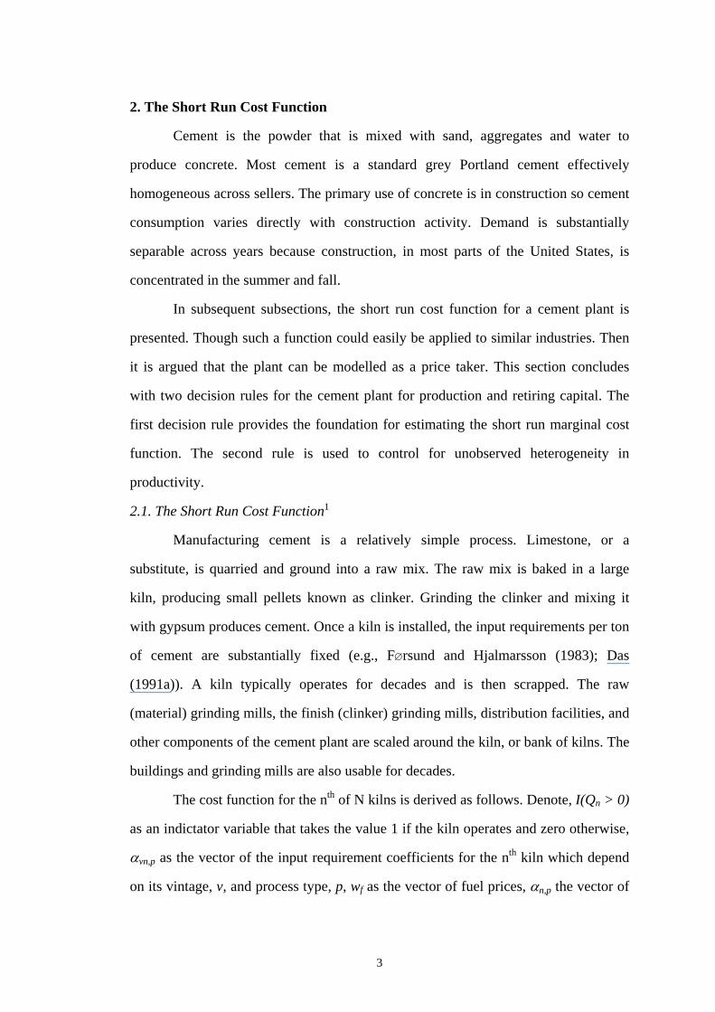
The cost function for the nth of N kilns is derived as follows. Denote, I(Qn > 0)

as an indictator variable that takes the value 1 if the kiln operates and zero otherwise,

αvn,p as the vector of the input requirement coefficients for the nth kiln which depend

on its vintage, v, and process type, p, wf as the vector of fuel prices, αn,p the vector of

3

the input requirement coefficients which do not depend on kiln vintage, wo as a vector

of other input prices and f*kn as the kiln specific fixed costs. The kiln cost function is

( ) ( ) { } (1) *0 , nnon,pnnpvnfnn kfQwQwQIw,QC +′+′×>= αα

Indexing kilns by vintage and type reflects the emphasis placed on these

characteristics in both the engineering and economics literature. There are three types

of kilns: wet process, dry process, and preheater/precalciner process kilns. Both fuel

and electricity requirements vary systematically by process. In particular, the wet

process features the highest fuel requirements, then the dry process, and then the

preheater/precalciner process kilns. Fuel consumption is also believed to increase

with the age of the kiln because of embodied technological change and depreciation

taking the form of increased input requirements (e.g., Das (1992); Rosenbaum

(1994)). Hence, fuel coefficients increase with age as follows:

…pvpvpv ,3,2,1 ααα << (2)

Kiln differences lead not only to variation across plants but within plants as

many plants operate multiple kilns of different vintages.2 Denote Q as plant output.

Hence, from equations (1) and (2), the short run marginal cost function is as follows:

⎪⎪⎪

⎩

⎪⎪⎪

⎨

⎧

∑=

<≤∑−

=′+′

+<≤′+′

<′+′

=n

iikQ

n

iik,pow,pvfw

kkQk,pow,pvfw

kQ,pow,pvfw

mc

1

1

1 3

211 2

1 1

αα

αα

αα

(3)

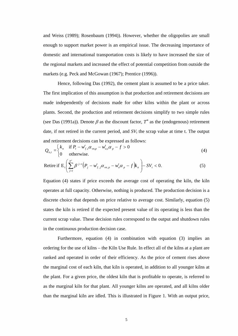
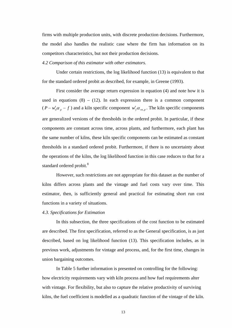
Hence marginal cost is a step function. For a plant with three kilns with capacities k1,

k2 and k3 plant marginal cost is depicted in Figure 1.

Fixed costs are composed of two components: start-up and expected shut

down costs, and non-sunk capital costs. Expenditure on the plant and equipment is

substantially sunk after installation because of the size and immobility of the kilns.

2.2. The Decision Variable of the Plant

The traditional view of the cement industry is that the combination of

economies of scale with high transportation costs creates within the US a set of

regional oligopolies (recent papers in this tradition include McBride (1983); Koller

4

and Weiss (1989); Rosenbaum (1994)). However, whether the oligopolies are small

enough to support market power is an empirical issue. The decreasing importance of

domestic and international transportation costs is likely to have increased the size of

the regional markets and increased the effect of potential competition from outside the

markets (e.g. Peck and McGowan (1967); Prentice (1996)).

Hence, following Das (1992), the cement plant is assumed to be a price taker.

The first implication of this assumption is that production and retirement decisions are

made independently of decisions made for other kilns within the plant or across

plants. Second, the production and retirement decisions simplify to two simple rules

(see Das (1991a)). Denote β as the discount factor, T* as the (endogenous) retirement

date, if not retired in the current period, and SVt the scrap value at time t. The output

and retirement decisions can be expressed as follows:

(4) otherwise. 0

0if = ,,

,⎩⎨⎧ >−′−′− fww P k

Q ptovn,ptftntn

αα

( ) (5) .0E if Retire ,,t <−⎟⎟⎠

⎞⎜⎜⎝

⎛−′−′−∑

∗

=

−t

T

tjnpopvnjfj

tj SVkfwwP ααβ

Equation (4) states if price exceeds the average cost of operating the kiln, the kiln

operates at full capacity. Otherwise, nothing is produced. The production decision is a

discrete choice that depends on price relative to average cost. Similarly, equation (5)

states the kiln is retired if the expected present value of its operating is less than the

current scrap value. These decision rules correspond to the output and shutdown rules

in the continuous production decision case.

Furthermore, equation (4) in combination with equation (3) implies an

ordering for the use of kilns – the Kiln Use Rule. In effect all of the kilns at a plant are

ranked and operated in order of their efficiency. As the price of cement rises above

the marginal cost of each kiln, that kiln is operated, in addition to all younger kilns at

the plant. For a given price, the oldest kiln that is profitable to operate, is referred to

as the marginal kiln for that plant. All younger kilns are operated, and all kilns older

than the marginal kiln are idled. This is illustrated in Figure 1. With an output price,

5

P, the first two kilns, with capacities k1 and k2, feature marginal costs below P and are

operated at full capacity. Kiln 2 is the marginal kiln. The third kiln, with a marginal

cost greater than P, is not operated.

Empirical support for the Kiln Use Rule is provided in Das (1992). After

allocating plant output to kilns according to the Kiln Use Rule, most kilns are found

to either operate at or near capacity or not at all.

The kiln retirement rule, equation (5), implies older kilns are retired before

newer kilns, and wet and dry process kilns are retired before preheater/precalciner

kilns. This pattern is generally observed over the sample period. However, there are

striking examples of new kilns being closed, and kilns more than 50 years old

continuing to operate. Anomalous plants must feature lower or higher than average

marginal costs or kiln fixed costs due to plant specific factors such as the quality of

their raw materials. The connection between plant productivity and plant exit has

been highlighted in recent work. Griliches and Regev (1995), working with a panel of

Israeli manufacturers, note plants closing during the sample period have significantly

lower labor productivity than other plants. Olley and Pakes (1996) estimate a

production function, including an adjustment for unobserved productivity differences

based on plant investment, and achieve significantly better results. In Section 4.4, the

kiln retirement rule is used to correct for the unobserved productivity differences

across plants.

Finally, it is worth noting some further characteristics of the equilibrium

underlying this characterisation of the industry. There may seem to be some tension

between the assumption of price taking behavior and observed extensive

heterogeneity as competition would drive out the more costly equipment and plants.

Salter (1966) resolves this tension. With expenditure on capital equipment at least

partially sunk, if demand exceeds capacity and price rises above average cost,

Ricardian rents will be earned. In Figure 1, the rent earned by the firm on each kiln is

equal to ( ) nnpopvnfn kfkwwPRT *, −′−′−= αα (6)

6

Unless entrants expect the rents subsequently earned by the kiln (or plant) will exceed

the sunk capital costs entry will not occur and there will be a price taking equilibrium,

with some plants earning Ricardian rents.

Specifying a complete theoretical expression for the Ricardian rents requires

specifying a general equilibrium model of the national market which is beyond the

scope of the paper. The rents depend on the characteristics of the kiln, the locational

advantage of the plant, and demand (see also Lindenberg and Ross (1981); Alchian

(1987)). A reduced form expression is presented in Section 4.4.

3. The Data

To estimate the decision rule for the plant, the operating status of each kiln

and a set of explanatory variables are required. The sample features an observation for

each plant for each year the plant is operable from 1977 to 1992. In this section, the

nature and sources of the data used in this paper are briefly described. First, the basic

set of data is described. The second subsection contains an outline of the method used

to extract the sample of the operating status for each kiln in each year and the

characteristics of the sample.

3.1. The Nature of the Data

Four broad sets of data are required: (1) prices of inputs, output and imported

cement (2) quantity of clinker produced (3) kiln and plant characteristics (4) quantity

of construction.

The price of cement, quantity produced of clinker and average number of kiln

maintenance days are obtained from the annual US Bureau of Mines Minerals

Yearbooks. Data on these variables are published for aggregates of small groups of

plants, usually adjacent to one another. The modal plant number for these aggregates

is 4 with 85% of the region years featuring 6 plants or less. The modal number of

kilns per group is 7 with 82% of the region years featuring 13 kilns or less. The

yearbook also contains the price of limestone (by state or substate) and import prices.3

The prices of other inputs, electricity, fuel and labor are obtained from various

US government reports. Again, where possible, for all states except Pennsylvania,

7

Texas and, to a lesser extent, California, these are aggregates over relatively small

numbers of plants or else averages across broader groupings.4

Plant and kiln characteristics are obtained from the annual Portland Cement

Association Plant Information Summary. This directory includes kiln capacities,

vintages, primary and supplementary types of fuels used and ownership. The directory

entries are crosschecked against the Minerals Yearbook regional plant and kiln

counts, trade journal reports and company annual reports.

Finally, the annual value of construction contracts data (by state) is obtained

from FW Dodge. This is deflated by the state construction price index constructed by

the author (see Prentice (1997) for more details).

It is important to note that all of this data is available to firms in the industry.

The government data is publically available. The Plant Information Summary and

construction data, are compiled explicitly for sale to industry participants and other

interested parties. Hence the model presented in Section 4 is usable by a firm or

consultant.

The data is summarized in Table 4 including the variables required for

controlling for Ricardian rents and unobserved heterogeneity across firms. These

variables are discussed in Sections 4.4 and 4.5.

The next step in assembling the data is to assign input and output prices, and

import prices, to plants. This yields a plant level data series by matching the state and

Minerals Yearbook region prices to the plants located within the relevant areas. For

assigning fuel prices to plants, the directory fuel reports are used unless contradicted

by a more reliable source.

At this point it is worth comparing this new dataset with those used by earlier

authors. This paper uses relatively disaggregated data rather than plant level data

available to Das ((1991a);(1991b)). Rather than using quantities of inputs and outputs

to estimate input requirement coefficients, as was done by Bertin, Bresnahan and Raff

(1996) and Das ((1991a;(1991b)), input and output prices are used. This makes the

problem more challenging as unlike input and output quantities, prices are determined

8

by factors independently of the technological characteristics of the firm. Estimating

input requirement parameters from input and output prices relies on duality

relationships.5 This dataset is, then, more like those used by Prentice (1996) and

Rosenbaum (1994).

This dataset improves on earlier data sets in two respects by including state

limestone price and wage rate series.6 The relatively disaggregated series constructed

for this paper are the best available series as plant level series are unavailable.

3.2. Calculating Kiln Operating Status

The operating status of each kiln cannot be determined by inspection of the

regional clinker output data (unlike for the steel mills in Bertin, Bresnahan and Raff

(1996)). So an algorithm is constructed to infer for each kiln at each plant whether the

kiln operated, did not operate or if its status was unknown. The algorithm is presented

in Table 1. The algorithm assumes the Kiln Use Rule holds at each plant but not

across plants. This is because, kilns of similar ages at different plants may have

different costs, because of different maintenance policies or raw material qualities, so

their operating status may differ.

The algorithm yields observations for 2154 marginal kilns (each one per plant

per year). All plants that featured kilns both operating and not operating, with the

differences in their vintages being less than or equal to two years, are deleted. One

plant featuring an unusual combination of processes, vintages and capacities is also

deleted. This leaves 1999 observations. The outcome for each plant can be

characterised into one of four groups, as recorded in Table 2.7

Table 3 demonstrates the different processes and vintages are all represented

in the sample.

4. The Econometric Model

In this section, the model presented in Section 2 is reconciled with the data to

yield a structural model of the short run cost function. Beginning with the production

decision rule, equation (4), it is argued that there is a common error term across the

kilns at a plant. This means for each plant the relevant observation is that for the

9

marginal kiln. The likelihood function for a new estimator required for this model is

derived. Then it is demonstrated that with some strong assumptions this model yields

the standard ordered probit. In Sections 4.4 and 4.5 it is discussed how to control for

unobserved heterogeneity and Ricardian rents.

4.1 Estimating a Cost function for a Discrete Production Process.

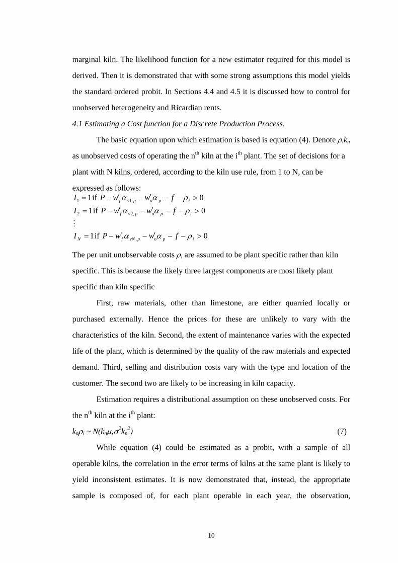
The basic equation upon which estimation is based is equation (4). Denote ρtkn

as unobserved costs of operating the nth kiln at the ith plant. The set of decisions for a

plant with N kilns, ordered, according to the kiln use rule, from 1 to N, can be

expressed as follows:

0 if 1

0 if 1

0 if 1

,

,22

,11

>−−′−′−=

>−−′−′−=

>−−′−′−=

ipopvNfN

ipopvf

ipopvf

fwwPI

fwwPI

fwwPI

ραα

ραα

ραα

The per unit unobservable costs ρi are assumed to be plant specific rather than kiln

specific. This is because the likely three largest components are most likely plant

specific than kiln specific

First, raw materials, other than limestone, are either quarried locally or

purchased externally. Hence the prices for these are unlikely to vary with the

characteristics of the kiln. Second, the extent of maintenance varies with the expected

life of the plant, which is determined by the quality of the raw materials and expected

demand. Third, selling and distribution costs vary with the type and location of the

customer. The second two are likely to be increasing in kiln capacity.

Estimation requires a distributional assumption on these unobserved costs. For

the nth kiln at the ith plant:

knρi ~ N(knµ,σ2kn2) (7)

While equation (4) could be estimated as a probit, with a sample of all

operable kilns, the correlation in the error terms of kilns at the same plant is likely to

yield inconsistent estimates. It is now demonstrated that, instead, the appropriate

sample is composed of, for each plant operable in each year, the observation,

10

associated with the marginal kiln. The likelihood function for estimating the short run

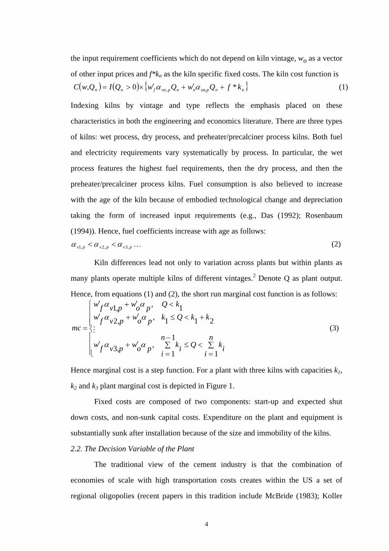
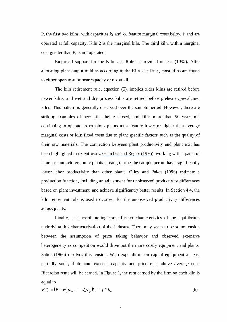
cost function is then developed. To aid the discussion, Figure 2 which contains a

density function for ρi when the plant has four kilns, is used. Along the horizontal

axis is the series of returns to operating each of the kilns. Costs that do not vary with

the kiln are removed for clarity. The return furthest to the right is that for the newest

kiln, denoted (A). Moving left along the horizontal axis are the returns for the second

(B), third (C) and fourth (D) ranked kilns.

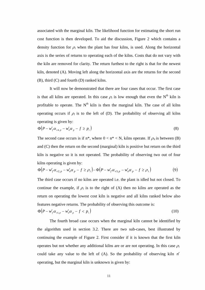
It will now be demonstrated that there are four cases that occur. The first case

is that all kilns are operated. In this case ρi is low enough that even the Nth kiln is

profitable to operate. The Nth kiln is then the marginal kiln. The case of all kilns

operating occurs if ρi is to the left of (D). The probability of observing all kilns

operating is given by: ( )ipopvf pfwwP ≥−′−′−Φ αα ,4 (8)

The second case occurs is if n*, where 0 < n* < N, kilns operate. If ρit is between (B)

and (C) then the return on the second (marginal) kiln is positive but return on the third

kiln is negative so it is not operated. The probability of observing two out of four

kilns operating is given by: ( ) ( ) ( )9 ,3,2 tpopvfipopvf fwwPfwwP ρααραα ≥−′−′−Φ−≥−′−′−Φ

The third case occurs if no kilns are operated i.e. the plant is idled but not closed. To

continue the example, if ρi is to the right of (A) then no kilns are operated as the

return on operating the lowest cost kiln is negative and all kilns ranked below also

features negative returns. The probability of observing this outcome is: ( )ipopvf pfwwP <−′−′−Φ αα ,1 (10)

The fourth broad case occurs when the marginal kiln cannot be identified by

the algorithm used in section 3.2. There are two sub-cases, best illustrated by

continuing the example of Figure 2. First consider if it is known that the first kiln

operates but not whether any additional kilns are or are not operating. In this case ρi

could take any value to the left of (A). So the probability of observing kiln n′

operating, but the marginal kiln is unknown is given by:

11

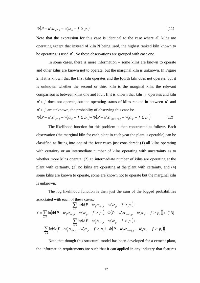
( )ipopvnf pfwwP ≥−′−′−Φ αα ,' (11)

Note that the expression for this case is identical to the case where all kilns are

operating except that instead of kiln N being used, the highest ranked kiln known to

be operating is used . So these observations are grouped with case one. n′

In some cases, there is more information – some kilns are known to operate

and other kilns are known not to operate, but the marginal kiln is unknown. In Figure

2, if it is known that the first kiln operates and the fourth kiln does not operate, but it

is unknown whether the second or third kiln is the marginal kiln, the relevant

comparison is between kilns one and four. If it is known that kiln operates and kiln

does not operate, but the operating status of kilns ranked in between n

n′

jn +′ ′ and

are unknown, the probablity of observing this case is: jn +′

( ) ( )ipopjnvfipopvnf fwwPfwwP ρααραα ≥−′−′−Φ−≥−′−′−Φ +′ ),(,' (12)

The likelihood function for this problem is then constructed as follows. Each

observation (the marginal kiln for each plant in each year the plant is operable) can be

classified as fitting into one of the four cases just considered: (1) all kilns operating

with certainty or an intermediate number of kilns operating with uncertainty as to

whether more kilns operate, (2) an intermediate number of kilns are operating at the

plant with certainty, (3) no kilns are operating at the plant with certainty, and (4)

some kilns are known to operate, some are known not to operate but the marginal kiln

is unknown.

The log likelihood function is then just the sum of the logged probabilities

associated with each of these cases: ( )

( ) (( )( )

( ) (( )∑∑

∑∑

∈+

∈

∈+

∈

≥−′−′−Φ−≥−′−′−Φ

+<−′−′−Φ

+≥−′−′−Φ−≥−′−′−Φ

+≥−′−′−Φ

=

4,,

3,1

2,1,

1,

ln

ln

ln

ln

iipopjvnfipopvnf

iipopvf

iipopvnfipopvnf

iipopvnf

pfwwPpfwwP

pfwwP

pfwwPpfwwP

pfwwP

αααα

αα

αααα

αα

)

)

(13)

Note that though this structural model has been developed for a cement plant,

the information requirements are such that it can applied in any industry that features

12

firms with multiple production units, with discrete production decisions. Furthermore,

the model also handles the realistic case where the firm has information on its

competitors characteristics, but not their production decisions.

4.2 Comparison of this estimator with other estimators.

Under certain restrictions, the log likelihood function (13) is equivalent to that

for the standard ordered probit as described, for example, in Greene (1993).

First consider the average return expression in equation (4) and note how it is

used in equations (8) – (12). In each expression there is a common component ( fwP po −′− α ) and a kiln specific component pvnfw ,α′ . The kiln specific components

are generalized versions of the thresholds in the ordered probit. In particular, if these

components are constant across time, across plants, and furthermore, each plant has

the same number of kilns, these kiln specific components can be estimated as constant

thresholds in a standard ordered probit. Furthermore, if there is no uncertainty about

the operations of the kilns, the log likelihood function in this case reduces to that for a

standard ordered probit.8

However, such restrictions are not appropriate for this dataset as the number of

kilns differs across plants and the vintage and fuel costs vary over time. This

estimator, then, is sufficiently general and practical for estimating short run cost

functions in a variety of situations.

4.3. Specifications for Estimation

In this subsection, the three specifications of the cost function to be estimated

are described. The first specification, referred to as the General specification, is as just

described, based on log likelihood function (13). This specification includes, as in

previous work, adjustments for vintage and process, and, for the first time, changes in

union bargaining outcomes.

In Table 5 further information is presented on controlling for the following:

how electricity requirements vary with kiln process and how fuel requirements alter

with vintage. For flexibility, but also to capture the relative productivity of surviving

kilns, the fuel coefficient is modelled as a quadratic function of the vintage of the kiln.

13

An attempt was made with an exponential specification but, even with well-behaved

simulated data, there were problems with convergence. The quadratic seemed the best

alternative to capture any non-linear relationship between fuel consumption and

vintage.

Furthermore, to attempt to capture productivity improvements following the

effective collapse of a strong trade union in the industry (Northrup (1989)), a scaled

trend is introduced. Finally, as discussed in sections 4.4 and 4.5, variables and terms

are introduced to control for unobserved heterogeneity across plants and to allow for

Ricardian rents.

The estimated coefficients may exceed industry averages, to be described in

more detail below, if there are significant components of the unobserved costs that

include labor, limestone, electricity and fuel, which cannot be ruled out.9

4.4 Controlling for unobserved heterogeneity across plants.

In section 2.2, it is noted that there are not infrequent examples of kilns not

being closed according to the kiln retirement rule, on the basis of their observable

characteristics. This suggested they had unobservable productivity differences. In this

section, a method to control for unobservable productivity differences is suggested.

First, define plants that closed earlier than would be expected by the vintage of

their kiln, relative to that of their neighbours as Exiters. Plants that remained open

with relatively old kilns are defined as Survivors. The second specification, to be

referred to as the Heterogeneity specification, allows for differences in the input

requirement coefficients of Exiters and Survivors.

Before discussing the construction of the survivor and exiter variables, the

nature of a near plant needs to be defined. If five or more plants are within 200 miles

of a plant, the five closest to the plant are considered near. The 1977 Census of

Transportation reports most cement is shipped within 200 miles of a plant. If there

were between one and four plants within 200 miles, these are considered the near

plants. If there are no plants within 200 miles, no near plant exists.

14

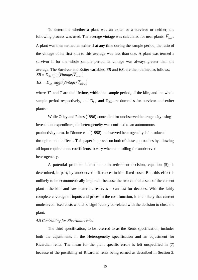
To determine whether a plant was an exiter or a survivor or neither, the

following process was used. The average vintage was calculated for near plants, nearV .

A plant was then termed an exiter if at any time during the sample period, the ratio of

the vintage of its first kiln to this average was less than one. A plant was termed a

survivor if for the whole sample period its vintage was always greater than the

average. The Survivor and Exiter variables, SR and EX, are then defined as follows: ( )

( )tnearTtEX

tnearTtSV

VVintageDEX

VageintVDSR

,

,

mean

min

∈

′∈

=

=

where T ′ and T are the lifetime, within the sample period, of the kiln, and the whole

sample period respectively, and DSV and DEX are dummies for survivor and exiter

plants.

While Olley and Pakes (1996) controlled for unobserved heterogeneity using

investment expenditure, the heterogeneity was confined to an autonomous

productivity term. In Dionne et al (1998) unobserved heterogeneity is introduced

through random effects. This paper improves on both of these approaches by allowing

all input requirements coefficients to vary when controlling for unobserved

heterogeneity.

A potential problem is that the kiln retirement decision, equation (5), is

determined, in part, by unobserved differences in kiln fixed costs. But, this effect is

unlikely to be econometrically important because the two central assets of the cement

plant - the kiln and raw materials reserves – can last for decades. With the fairly

complete coverage of inputs and prices in the cost function, it is unlikely that current

unobserved fixed costs would be significantly correlated with the decision to close the

plant.

4.5 Controlling for Ricardian rents.

The third specification, to be referred to as the Rents specification, includes

both the adjustments in the Heterogeneity specification and an adjustment for

Ricardian rents. The mean for the plant specific errors is left unspecified in (7)

because of the possibility of Ricardian rents being earned as described in Section 2.

15

While a formal expression is not possible, it is expected the rents vary positively with

demand, D, the price of imported cement, Pm, the distance from domestic competition,

DFC, the distance from import competition, DFCD and negatively with vintage,

Vintage. A reduced form expression for the Ricardian rents is reported in Table 5.

5. Results

The results of estimating the three specifications are discussed as follows.

First, the estimates of the input requirement coefficients in the General and

Heterogeneity specifications are presented, followed by a discussion of the effects of

controlling for Survivors and Exiters. Finally, the effects of including variables to

capture the Ricardian rents are discussed.

In Table 6 industry averages of the input requirement coefficients followed by

estimates obtained from each of the three specifications are presented. The industry

averages are calculated from national input consumption and production statistics

from the Bureau of Mines Minerals Yearbooks or, for fuel consumption, from 1977-

1988, from surveys reported therein. As long as there is not too much dispersion in

the distribution, these averages can be used as a benchmark for assessing the

reasonableness of the estimates. While it is unlikely the estimated coefficients are

exactly the same as these averages it is expected that the differences between them

and the industry averages are statistically insignificant. For each variable the

coefficient value, the standard error (in parentheses) and the t-statistic are reported.

The estimated limestone and electricity requirement coefficients are typically

much greater than the industry averages, though the differences, for several of these

coefficients, are statistically insignificant. The relative sizes of the estimated

coefficients for electricity by process for the first two specifications are also counter

intuitive though, again, the differences are statistically insignificant. The coefficients

on labor, before the change in bargaining, are more satisfactory in that they are not

significantly different from the industry averages but they are also not significantly

different from zero.

16

The standard errors of the regressions for the General and Heterogeneity

specifications are relatively high. With annual average real prices of cement varying

between $70.11 and $41.02, standard errors in the low to mid twenties seem too large,

suggesting considerable variation is not being picked up by the model. A likelihood

ratio test shows introducing the additional variables in the Heterogeneity specification

results in a significant improvement on the General specification.

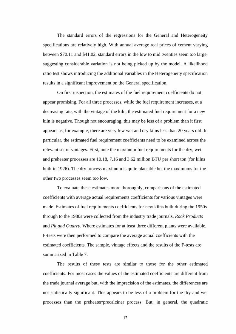
On first inspection, the estimates of the fuel requirement coefficients do not

appear promising. For all three processes, while the fuel requirement increases, at a

decreasing rate, with the vintage of the kiln, the estimated fuel requirement for a new

kiln is negative. Though not encouraging, this may be less of a problem than it first

appears as, for example, there are very few wet and dry kilns less than 20 years old. In

particular, the estimated fuel requirement coefficients need to be examined across the

relevant set of vintages. First, note the maximum fuel requirements for the dry, wet

and preheater processes are 10.18, 7.16 and 3.62 million BTU per short ton (for kilns

built in 1926). The dry process maximum is quite plausible but the maximums for the

other two processes seem too low.

To evaluate these estimates more thoroughly, comparisons of the estimated

coefficients with average actual requirements coefficients for various vintages were

made. Estimates of fuel requirements coefficients for new kilns built during the 1950s

through to the 1980s were collected from the industry trade journals, Rock Products

and Pit and Quarry. Where estimates for at least three different plants were available,

F-tests were then performed to compare the average actual coefficients with the

estimated coefficients. The sample, vintage effects and the results of the F-tests are

summarized in Table 7.

The results of these tests are similar to those for the other estimated

coefficients. For most cases the values of the estimated coefficients are different from

the trade journal average but, with the imprecision of the estimates, the differences are

not statistically significant. This appears to be less of a problem for the dry and wet

processes than the preheater/precalciner process. But, in general, the quadratic

17

functional form appears to be too restrictive to capture the variation in fuel

requirements with vintage. Furthermore, a common vintage effect may also not be

appropriate – especially for the preheater/precalciner kilns.

For labor requirements, after the change in bargaining arrangements, statistics

similar to those calculated in Table 7 are calculated, adding in just the, near

significant, squared component of the coefficient. The results are similar with the

implied increase in productivity being too large and occurring too quickly. From four

(General) to six (Heterogeneity) years after the change the estimated labor

requirements coefficients are negative.

Next the adjustments to the input requirement coefficients for the different

requirements for survivor and exiter plants are summarized in Table 8. The survivor

and exiter adjustment coefficients are tested for being significantly less than and

significantly greater than zero where applicable.

Though introducing these variables significantly improved the specification,

none of the individual coefficients are significantly different from zero in the

hypothesized direction. The coefficient on electricity for the exiters is even

significantly negative though this may reflect that low electricity consuming wet

process plants were exiting early in the period. The sizes of the fuel coefficients for

the survivors and exiters are plausible, though both are imprecisely estimated.

Finally, the effects of controlling for Ricardian rents are considered. Though a

likelihood ratio test results in a significant improvement of the specification, the

standard error on the regression increases considerably. The estimated standard error

was expected to decrease if the large size of the standard error in the earlier

specifications was due to failing to capture variations in rents. Furthermore, with the

exception of limestone, the sizes and signs of the input requirement coefficients all

become much less plausible. The value of the constant term is unreasonably high.

Likewise the sizes of the coefficients on the adjustment coefficients for survivors and

exiters are less plausible. The coefficients on the rental variables are all insignificant.

18

The result of the likelihood ratio test suggests something is being picked up but it

does not appear to be Ricardian rents.

To sum up, there are two features of the results that are encouraging and one

less encouraging. The first encouraging feature is that the specification is basically

supported by the data as the new estimator is successfully estimated. The second

encouraging feature is that many of the estimated coefficients are not significantly

different from the industry averages. The less encouraging feature is that the

differences from the industry averages seem too large to be attributed to a non-

symmetric distribution of coefficients. Perhaps the most problematic component is the

estimated fuel requirement coefficients. They are plausible over certain ranges of

vintages, especially for the wet and dry process kilns. However, the quadratic

relationship with vintage appears to be too restrictive. Introducing adjustment

coefficients for survivor and exiter plants significantly improves the specification as a

whole but the individual adjustment coefficients are not significantly different from

zero as hypothesized. Finally, introducing the reduced form measure of Ricardian

rents also improves the specification as a whole, but the additional variables are

insignificant and the plausibility of the results in general deteriorates, which suggests

this is the least successful component of the estimation. Collinearity may be a

problem here.

So, for future work, there are several ways in which the specification could be

improved. First, a more flexible specification of the relationship between fuel

consumption and kiln vintage could be used. Second, alternative specifications of the

rent variables could be introduced. Third, the specification of the variance could be

adjusted to control for the effects of exit and entry.

There are echoes of these findings in earlier work. Rosenbaum (1994) reported

negative coefficients on a measure of vintage (which would trend downwards in his

sample) and on wage rates. It would be interesting to see if Rosenbaum's measure of

wages was also trending downwards. The use of the earlier part of the sample period

may have avoided this problem with fuel prices. Prentice (1996), for the same sample

19

period, had reversed coefficient sizes on variables capturing the interaction of fuel

prices with process types. Das (1991a) had a constant term that was too high. Also,

her results, using the prices data, improved when she shifted from using a logit to a

semi-parametric estimation technique. The work of Rosenbaum and Das, to a certain

extent, through their different sample periods, may have been insulated from the

problems with either specification or unobserved variables that seem to be a

problematic feature of these results.

6. Conclusion

This paper presents a structural model of a short run cost function for an

industry with two features, recently highlighted in the literature, that make using

existing techniques problematic: discrete production decisions and unobserved

heterogeneity. Handling discrete production decisions requires a new estimator, of

which the ordered probit is a special case. This estimator is extended to handle

incomplete information on firm production decisions – a realistic constraint on firms

and consultants. Data on plant survival and exit is used to adjust all input requirement

coefficients for unobserved heterogeneity in productivity. The structural model is

successfully estimated using a new dataset on the U.S. Portland cement industry.

Furthermore, many of the estimates of the coefficients of the cost function are not

significantly different from independent estimates derived from trade journals and

input consumption statistics. However, the differences between the estimates and the

industry averages are too great to be completely comfortable. This, with the mixed

success in controlling for unobserved heterogeneity and Ricardian rents, suggests that

though the approach taken in this paper is promising more work needs to be done.

20

References

Alchian, A. (1987), 'Rents', in J. Eatwell, M. Milgate and P. Newman (eds.) The New

Palgrave: A Dictionary of Economics, Vol. 4, Macmillan, London.

Bertin, A. L., T. F. Bresnahan and D. M.G. Raff (1996), 'Localized Competition and

the Aggregation of Plant-level Increasing Returns: Blast Furnaces 1929--

1935', Journal of Political Economy, 104, 241-266.

Bresnahan, T. F. (1989), 'Empirical Studies of Industries with Market Power', in R.

Schmalansee and R. D. Willig (eds.), Handbook of Industrial Organization,

Vol. 2, North-Holland, New York.

Bresnahan, T. F. and V. A. Ramey (1994), 'Output Fluctuations at the Plant Level',

Quarterly Journal of Economics, 109, 593-624.

Bresnahan, T. F. and P. C. Reiss (1990), 'Entry in Monopoly Markets', Review of

Economic Studies, 57, 531-553.

Bureau of Labor Statistics (various years), Employment, Hours and Earnings, G.P.O,

Washington DC.

Bureau of Mines (1976-1992), chapters on Cement and Crushed Stone in Minerals

Yearbook, G.P.O, Washington DC.

Capone Jr., C. A. and K. G. Elzinga (1987), 'Technology and Energy Use Before,

During and After OPEC: The U.S. Portland Cement Industry', The Energy

Journal, 8, 93-112.

Das, S. (1991a), 'A semiparametric structural analysis of the idling of cement kilns',

Journal of Econometrics, 50, 235-256.

_____ (1991b), 'Estimation of Fuel Coefficients of Cement Production: A Fixed-

Effects Approach to Nonlinear Regression', Journal of Business & Economic

Statistics, 9, 469-474.

_____ (1992), 'A Microeconometric Model of Capital Utilization and Retirement: The

Case of the U.S Cement Industry', Review of Economic Studies, 59, 277-297.

21

Davis, S. J. and J. Haltiwanger (1992), 'Gross Job Creation, Gross Job Destruction,

and Employment Reallocation', Quarterly Journal of Economics, 107, 819-

863.

Dionne, G., R. Gagné, C. Vanasse (1998), 'Inferring technological parameters from

incomplete panel data', Journal of Econometrics, 87, 303 –327.

Department of Commerce (various, a), County Business Patterns, G.P.O, Washington

DC.

Department of Commerce (various, b), U.S. Census of Manufactures, G.P.O,

Washington DC.

Department of Energy (various), State Energy Price and Expenditure Report, G.P.O,

Washington DC.

Fφrsund, F. R. and L. Hjalmarsson (1983), 'Technical Progress and Structural Change

in the Swedish Cement Industry 1955-1979', Econometrica, 51, 1449-1467.

Greene, W. H. (1993), Econometric Analysis, 2nd Edition, Macmillan Publishing

Company, New York.

Griliches, Z. and H. Regev (1995), 'Firm Productivity in Israeli Industry 1979-1988',

Journal of Econometrics, 65, 175-203.

Koller II, R. H. and L. W. Weiss (1989), 'Price Levels and Seller Concentration: The

Case of Portland Cement' in L. W. Weiss (ed.), Concentration and Price, MIT

Press, Cambridge.

Lindenberg, E. B. and S. A. Ross (1981), 'Tobin's q Ratio and Industrial

Organization', Journal of Business, 54, 1-32.

McBride, M. E. (1983), 'Spatial Competition and Vertical Integration: Cement and

Concrete Revisited', American Economic Review, 73, 1011-1022.

Northrup, H. R. (1989), 'From Union Hegemony to Union Disintegration: Collective

Bargaining in Cement and Related Industries', Journal of Labor Research, 10,

339-376.

Olley, G. S. and A. Pakes (1996), 'The Dynamics of Productivity in the

Telecommunications Equipment Industry', Econometrica, 64, 1263-1297.

22

Peck, M. J. and J. J. McGowan (1967), 'Vertical Integration in Cement: A Critical

Examination of the FTC Staff Report', Antitrust Bulletin, 12, 505-531.

Peray, K. E. (1986), The Rotary Cement Kiln, 2nd Edition, Chemical Publishing Co.,

New York.

Portland Cement Association (1974-1992), U.S. and Canadian Portland Cement

Industry: Plant Information Summary, Portland Cement Association, Skokie.

Prentice, D. (1996), The Dramatic, Mysterious Increase in Imports of Portland

Cement into the U.S., mimeo, Yale University.

__________ (1997), Import Competition in the U.S. Portland Cement Industry, Ph. D.

Thesis, Yale University.

__________ (1998), A microeconometric model of a short run cost function with

unobserved heterogeneity, La Trobe University School of Business Discussion

Paper A98.01.

Rosenbaum, D. I. (1994), 'Efficiency v. Collusion: Evidence Cast in Cement', Review

of Industrial Organization, 9, 379-392.

Salter, W. E. G. (1966), Productivity and Technical Change, Cambridge University

Press, Cambridge.

23

Endnotes

1. This section is based on Das (1992) and Peray (1986). See Prentice (1998) for more

details on the engineering characteristics of cement production.

2. A few plants have kilns of multiple processes but the ordering by vintage achieves

the same ordering i.e. preheater/precalciner kilns are almost always newer than dry or

wet process kilns in the same plant.

3. Import prices are by customs district (see Bureau of Mines (1976 – 1992) for more

details) and are assigned to plants similar to the state case.

4. For fuel and electricity prices, Department of Energy (various), for wage rates see

Bureau of Labor Statistics (various), Bureau of the Census ((various, a);(various, b)).

See also Prentice (1997).

5. Discreteness violates the usual conditions under which duality relationships hold.

However, at the kiln level, the usual relationships hold which enable use of duality.

6. Capone and Elzinga (1987) used national limestone prices. Substantially national

cement industry wage rates or even broader aggregates were used by Das (various)

and Rosenbaum (1994; and earlier papers). For some of these variables there are

missing observations. In some cases, missing observations are replaced using data

from adjacent or similar plants, similar variables, or interpolated.

7. Das (1992) used the Kiln Use Rule to infer kiln operations using plant level data. In

an improvement on the methods used by Das, I corrected the capacity statistics for

counter-cyclical maintenance. Not making this correction could lead to

overestimating the number of kilns operating in boom periods, and underestimating

the number of kilns operating in slower periods.

8. These conditions were satisified sufficiently for Bresnahan and Reiss (1990) to

infer distributions of fixed costs from entry decisions and for Bertin, Bresnahan and

Raff (1996) to estimate expected production rates.

9. Note that the estimate of the standard error of the distribution will, at best, provide

an upper bound on the standard error of the underlying errors ρ. As long as the

deviations from the reduced form estimate of the rents are normally distributed and

24

uncorrelated with ρ the estimated standard error will be an estimate of the sum of the

square root of the sum of the variances for the two normal distributions.

25

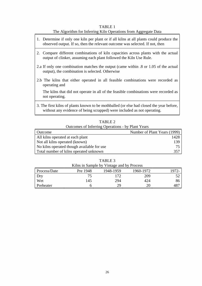
TABLE 1 The Algorithm for Inferring Kiln Operations from Aggregate Data

1. Determine if only one kiln per plant or if all kilns at all plants could produce the observed output. If so, then the relevant outcome was selected. If not, then

2. Compare different combinations of kiln capacities across plants with the actual output of clinker, assuming each plant followed the Kiln Use Rule.

2.a If only one combination matches the output (came within .8 or 1.05 of the actual output), the combination is selected. Otherwise

2.b The kilns that either operated in all feasible combinations were recorded as operating and

The kilns that did not operate in all of the feasible combinations were recorded as not operating.

3. The first kilns of plants known to be mothballed (or else had closed the year before, without any evidence of being scrapped) were included as not operating.

TABLE 2

Outcomes of Inferring Operations - by Plant Years Outcome Number of Plant Years (1999)All kilns operated at each plant 1428Not all kilns operated (known) 139No kilns operated though available for use 75Total number of kilns operated unknown 357

TABLE 3

Kilns in Sample by Vintage and by Process Process/Date Pre 1948 1948-1959 1960-1972 1972-Dry 75 172 209 52Wet 145 294 424 86Preheater 6 29 20 487

26

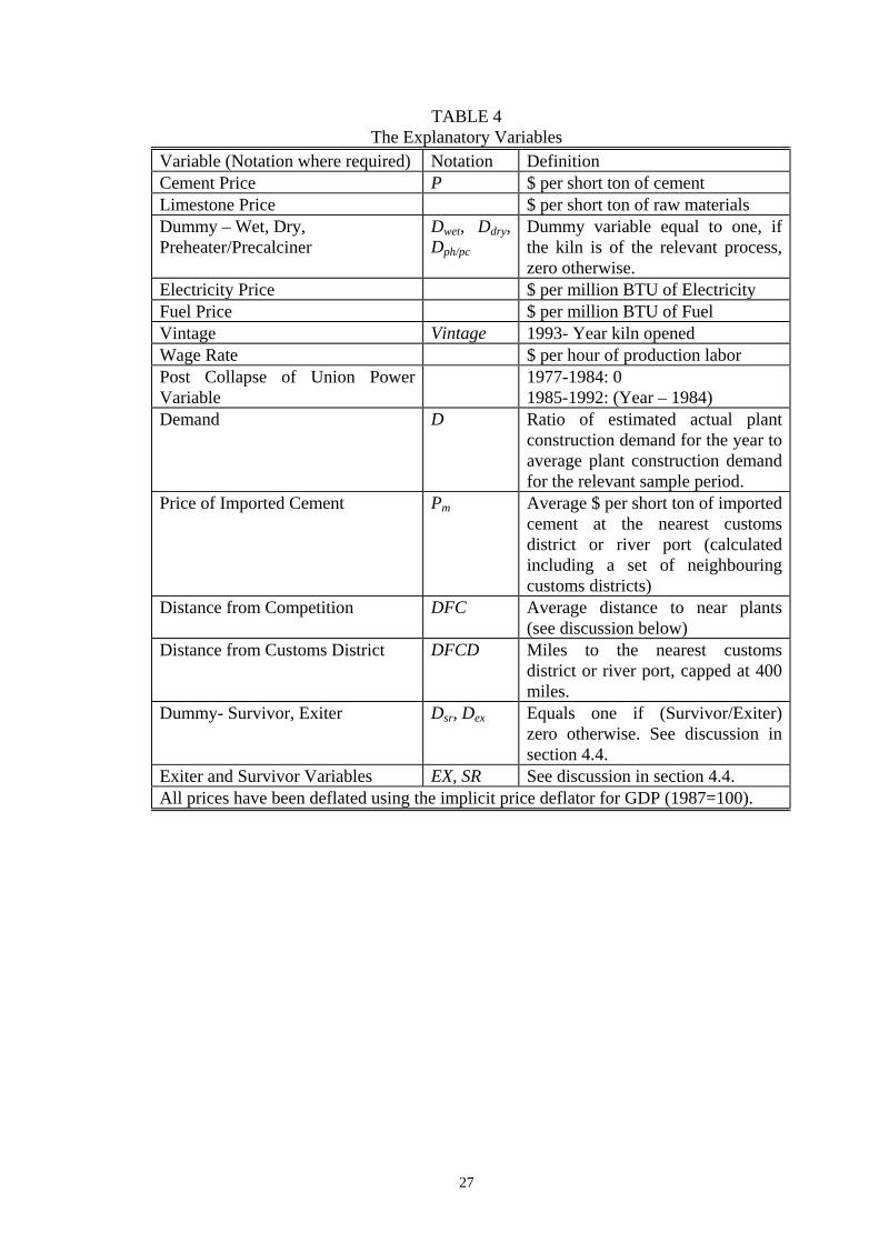
TABLE 4 The Explanatory Variables

Variable (Notation where required) Notation Definition Cement Price P $ per short ton of cement Limestone Price $ per short ton of raw materials Dummy – Wet, Dry, Preheater/Precalciner

Dwet, Ddry, Dph/pc

Dummy variable equal to one, if the kiln is of the relevant process, zero otherwise.

Electricity Price $ per million BTU of Electricity Fuel Price $ per million BTU of Fuel Vintage Vintage 1993- Year kiln opened Wage Rate $ per hour of production labor Post Collapse of Union Power Variable

1977-1984: 0 1985-1992: (Year – 1984)

Demand D Ratio of estimated actual plant construction demand for the year to average plant construction demand for the relevant sample period.

Price of Imported Cement Pm Average $ per short ton of imported cement at the nearest customs district or river port (calculated including a set of neighbouring customs districts)

Distance from Competition DFC Average distance to near plants (see discussion below)

Distance from Customs District DFCD Miles to the nearest customs district or river port, capped at 400 miles.

Dummy- Survivor, Exiter Dsr, Dex Equals one if (Survivor/Exiter) zero otherwise. See discussion in section 4.4.

Exiter and Survivor Variables EX, SR See discussion in section 4.4. All prices have been deflated using the implicit price deflator for GDP (1987=100).

27

TABLE 5 Specification of the Variable Coefficients and Ricardian Rents

Coefficient for Specification Included in the General Specification

Electricity αe,wet Dwet+ αe,dry(Ddry + Dph/pc) Fuel αf,wet Dwet+ αf,dryDdry + αf,ph/pcDph/pc + αv1Vintage + αv2Vintage2

Labor αlabor + αb1Db(Year-1984) + αb2Db(Year-1984)2

Added with the Heterogeneity Specification

Limestone, Fuel, Electricity, Labor

αinput + αex,inputDexEX + αsv,inputDsvSR

Added with the Rents Specification

RTnt µdD + µmPm + µdfcDFC + µdfcdDFCD + µvVintagen All variables are defined in Section 3

28

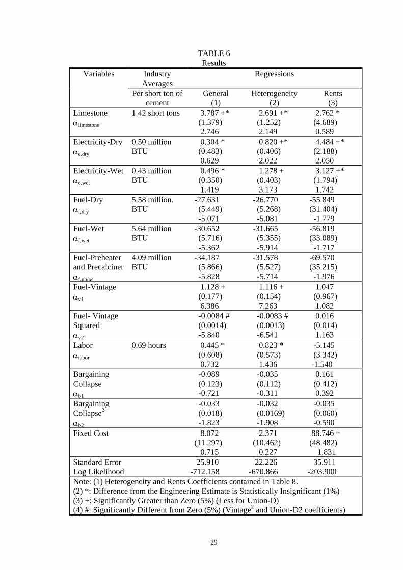
TABLE 6 Results

Industry Averages

Regressions Variables

Per short ton of cement

General (1)

Heterogeneity (2)

Rents (3)

Limestone αlimestone

1.42 short tons 3.787 +* (1.379) 2.746

2.691 +* (1.252) 2.149

2.762 * (4.689) 0.589

Electricity-Dry αe,dry

0.50 million BTU

0.304 * (0.483) 0.629

0.820 +* (0.406) 2.022

4.484 +* (2.188) 2.050

Electricity-Wet αe,wet

0.43 million BTU

0.496 * (0.350) 1.419

1.278 + (0.403) 3.173

3.127 +* (1.794) 1.742

Fuel-Dry αf,dry

5.58 million. BTU

-27.631 (5.449) -5.071

-26.770 (5.268) -5.081

-55.849 (31.404) -1.779

Fuel-Wet αf,wet

5.64 million BTU

-30.652 (5.716) -5.362

-31.665 (5.355) -5.914

-56.819 (33.089) -1.717

Fuel-Preheater and Precalciner αf,ph/pc

4.09 million BTU

-34.187 (5.866) -5.828

-31.578 (5.527) -5.714

-69.570 (35.215) -1.976

Fuel-Vintage αv1

1.128 + (0.177) 6.386

1.116 + (0.154) 7.263

1.047 (0.967) 1.082

Fuel- Vintage Squared αv2

-0.0084 # (0.0014) -5.840

-0.0083 # (0.0013) -6.541

0.016 (0.014) 1.163

Labor αlabor

0.69 hours 0.445 * (0.608) 0.732

0.823 * (0.573) 1.436

-5.145 (3.342) -1.540

Bargaining Collapse αb1

-0.089 (0.123) -0.721

-0.035 (0.112) -0.311

0.161 (0.412) 0.392

Bargaining Collapse2

αb2

-0.033 (0.018) -1.823

-0.032 (0.0169) -1.908

-0.035 (0.060) -0.590

Fixed Cost 8.072 (11.297) 0.715

2.371 (10.462) 0.227

88.746 + (48.482) 1.831

Standard Error 25.910 22.226 35.911 Log Likelihood -712.158 -670.866 -203.900 Note: (1) Heterogeneity and Rents Coefficients contained in Table 8. (2) *: Difference from the Engineering Estimate is Statistically Insignificant (1%) (3) +: Significantly Greater than Zero (5%) (Less for Union-D) (4) #: Significantly Different from Zero (5%) (Vintage2 and Union-D2 coefficients)

29

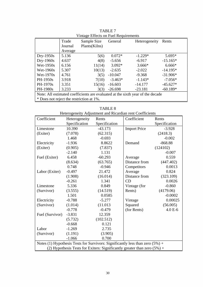
TABLE 7

Vintage Effects on Fuel Requirements Trade

Journal Average

Sample Size Plants(Kilns)

General Heterogeneity Rents

Dry-1950s 5.136 5(6) 0.072* -1.229* 5.695* Dry-1960s 4.637 4(8) -5.656 -6.917 -15.165* Wet-1950s 6.156 11(14) 3.092* 3.666* 6.666* Wet-1960s 5.307 10(13) -2.635 -2.022 -14.195* Wet-1970s 4.761 3(5) -10.047 -9.368 -31.906* PH-1950s 3.918 7(10) -3.463* -1.143* -7.056* PH-1970s 3.351 15(16) -16.603 -14.177 -45.627* PH-1980s 3.233 3(3) -26.698 -23.181 -60.189* Note: All estimated coefficients are evaluated at the sixth year of the decade * Does not reject the restriction at 1%.

TABLE 8 Heterogeneity Adjustment and Ricardian rent Coefficients

Coefficient Heterogeneity Specification

Rents Specification

Coefficient Rents Specification

Limestone (Exiter)

10.390 (7.078) 1.468

-43.173 (62.315) -0.693

Import Price -3.928 (2418.3) -0.002

Electricity (Exiter)

-1.936 (0.905) -2.140

8.8622 (7.837) 1.131

Demand -868.88 (124102) -0.007

Fuel (Exiter) 6.458 (8.634) 0.748

-60.293 (63.765) -0.946

Average Distance from Competitors

0.559 (447.402) 0.0013

Labor (Exiter) -0.497 (1.908) -0.261

21.472 (16.014) 1.341

Average Distance from CD

0.824 (323.109) 0.0026

Limestone (Survivor)

5.336 (3.555) 1.501

0.849 (14.519) 0.0585

Vintage (for Rents)

-0.860 (4179.06) -0.0002

Electricity (Survivor)

-0.788 (1.014) -0.778

-5.277 (11.013 -0.479

Vintage Squared (for Rents)

0.00025 (56.005) 4.0 E-6

Fuel (Survivor) -3.831 (5.732) -0.668

12.359 (102.512) 0.121

Labor (Survivor)

-1.269 (1.191) -1.066

2.735 (3.905) 0.700

Notes (1) Hypothesis Tests for Survivors: Significantly less than zero (5%) + (2) Hypothesis Tests for Exiters: Significantly greater than zero (5%) +

30

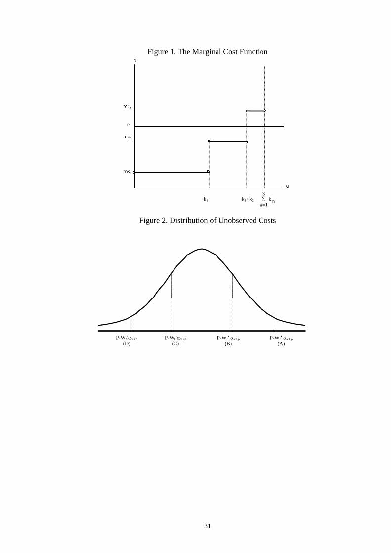
Figure 1. The Marginal Cost Function

k1 k1+k2 ∑=

3

1nk

n

Figure 2. Distribution of Unobserved Costs

P-Wf’αv3,p

(D) P-Wf’αv3,p

(C) P-Wf’ αv2,p

(B) P-Wf’ αv1,p

(A)

31