A Methodology to Estimate Load and Non-Load Shares of Highway Pavement Routine Maintenance and...
179
FHWA/IN/JTRP-2000/4 Final Report A METHODOLOGY TO ESTIMATE LOAD AND NON-LOAD SHARES OF HIGHWAY PAVEMENT ROUTINE MAINTENANCE AND REHABILITATION EXPENDITURES Zongzhi Li Kumares C. Sinha April 2000
Transcript of A Methodology to Estimate Load and Non-Load Shares of Highway Pavement Routine Maintenance and...

FHWA/IN/JTRP-2000/4 Final Report A METHODOLOGY TO ESTIMATE LOAD AND NON-LOAD SHARES OF HIGHWAY PAVEMENT ROUTINE MAINTENANCE AND REHABILITATION EXPENDITURES Zongzhi Li Kumares C. Sinha April 2000

FINAL REPORT
FHWA/IN/JTRP-2000/4
A METHODOLOGY TO ESTIMATE LOAD AND NON-LOAD SHARES OF HIGHWAY PAVEMENT ROUTINE MAINTENANCE AND
REHABILITATION EXPENDITURES
by
Zongzhi Li Graduate Research Assistant
and Kumares C. Sinha
Professor of Civil Engineering
Purdue University School of Civil Engineering
Joint Transportation Research Program Project No.: C-36-54DDD
File No.3-3-56 SPR-2332
Prepared in Cooperation with the Indiana Department of Transportation and
The U.S. Department of Transportation Federal Highway Administration
The contents of this report reflect the views of the authors who are responsible for the facts and the accuracy of the data presented herein. The contents do not necessarily reflect the official views of the Federal Highway Administration and the Indiana Department of Transportation. This report does not constitute a standard, a specification, or a regulation.
Purdue University West Lafayette, Indiana 47907
April 2000

15-2 4/00 JTRP-2000/4 INDOT Division of Research West Lafayette, IN 47906
INDOT Research
TECHNICAL Summary Technology Transfer and Project Implementation Information
TRB Subject Code: 15-2 Cost Allocation April 2000 Publication No.: FHWA/IN/JTRP-2000/4, SPR-2332 Final Report
A METHODOLOGY TO ESTIMATE LOAD AND NON-LOAD SHARES OF HIGHWAY PAVEMENT ROUTINE MAINTENANCE
AND REHABILITATION EXPENDITURES Introduction
A critical component of a highway cost allocation study is to determine the cost responsibilities of various vehicle classes related to highway pavement maintenance and rehabilitation expenditures. In the past, the load and non-load shares of maintenance and rehabilitation expenditures were determined using a number of approaches, ranging from arbitrary percentages to rational assumptions. As pavement maintenance and rehabilitation continue to increase as a portion of annual highway expenditures, the
development of an improved procedure to address the issue of load and non-load shares of such expenditures has become more important. The scope of the present study includes the development of appropriate econometric models to relate pavement maintenance and rehabilitation expenditures to traffic loading and various non-load factors. The models are then used to estimate the shares of load and non-load factors.
Findings The study revealed that the shares
of pavement repair expenditures attributable to load and non-load factors depend on several factors, such as the type of improvement (routine maintenance or rehabilitation), pavement type, and other variables. For routine maintenance, the load and non-load shares were found to be 25-75 for flexible pavements, 36-64 and 60-40 for Jointed Concrete Pavements (JCP) and Continuously Reinforced Concrete (CRC)
pavements, and 30-70 for composite pavements. The load and non-load fractions of rehabilitation expenditures used to repair pavement damage were found to be 30-70 for flexible pavements, 80-20 for JCP, and 40-60 for composite pavements. It is expected that the results of this study would facilitate the apportionment of pavement maintenance and rehabilitation expenditures in a fair and equitable manner.
Implementation In the present study, it was revealed that the load shares of pavement maintenance and rehabilitation expenditures for flexible and composite pavements were lower than those for rigid pavements, regardless of pavement repair category. Furthermore, for each pavement type, it was found that pavement segments that had received non-structural repairs (i.e., routine maintenance) had a relatively smaller load
share of repair expenditures as compared to those segments that had received structure-enhancing repairs (rehabilitation). In light of the discussion of results, it is imperative that any meaningful and reliable highway cost allocation study be preceded by determination of the load and non-load shares of pavement maintenance and rehabilitation expenditures. This should be carried out with respect to the type of

15-2 4/00 JTRP-2000/4 INDOT Division of Research West Lafayette, IN 47906
pavements in the network in question and the various categories of past pavement repair activities. It should also utilize, as much as possible, current data on the network usage, condition, and maintenance expenditures. The observations and results
from this study can be salient inputs for the update of the highway cost allocation study for Indiana, particularly in allocating pavement maintenance and rehabilitation expenditures.
Contact For more information: Prof. Kumares Sinha Principal Investigator School of Civil Engineering Purdue University West Lafayette IN 47907 Phone: (765) 494-2204 Fax: (765) 496-1105
Indiana Department of Transportation Division of Research 1205 Montgomery Street P.O. Box 2279 West Lafayette, IN 47906 Phone: (765) 463-1521 Fax: (765) 497-1665 Purdue University Joint Transportation Research Program School of Civil Engineering West Lafayette, IN 47907-1284 Phone: (765) 494-9310 Fax: (765) 496-1105

iii
TECHNICAL REPORT STANDARD TITLE PAGE
1. Report No. 2. Government Accession No.
3. Recipient's Catalog No.
FHWA/IN/JTRP-2000/4
4. Title and Subtitle A Methodology to Estimate Load and Non-Load Shares of Highway Pavement Routine Maintenance and Rehabilitation Expenditures
5. Report Date April 2000
6. Performing Organization Code 7. Author(s) Zongzhi Li and Kumares Sinha
8. Performing Organization Report No. FHWA/IN/JTRP-2000/4
9. Performing Organization Name and Address Joint Transportation Research Program 1284 Civil Engineering Building Purdue University West Lafayette, Indiana 47907-1284
10. Work Unit No.
11. Contract or Grant No. SPR-2332
12. Sponsoring Agency Name and Address Indiana Department of Transportation State Office Building 100 North Senate Avenue Indianapolis, IN 46204
13. Type of Report and Period Covered
Final Report
14. Sponsoring Agency Code
15. Supplementary Notes Prepared in cooperation with the Indiana Department of Transportation and Federal Highway Administration. 16. Abstract
The present study focused on the estimation of load and non-load shares of pavement maintenance and rehabilitation expenditures. The information provides the basis for the allocation of pavement-related expenditures in a highway cost allocation study. A comprehensive database was developed in the study, and an aggregate performance approach was used based on econometric models. This approach utilizes the marginal effect of traffic loading to quantify the load and non-load shares of pavement routine maintenance and rehabilitation expenditures. The study revealed that the share of pavement damage attributable to load and non-load factors depends on several factors such as the type of improvement (routine maintenance or rehabilitation), pavement type, and other variables. For routine maintenance, the load and non-load shares were found to be 25-75 for flexible pavements, 36-64 and 60-40 for Jointed Concrete Pavements (JCP) and Continuously Reinforced Concrete (CRC) pavements, and 30-70 for composite pavements. The load and non-load fractions of rehabilitation expenditures used to repair pavement damage were found to be 30-70 for flexible pavements, 80-20 for JCP, and 40-60 for composite pavements. It is expected that the results of this study will facilitate the apportionment of pavement routine maintenance and rehabilitation expenditures in a fair and equitable manner.
17. Key Words Highway cost allocation, load and non-load shares, pavement routine maintenance and rehabilitation, flexible pavements, rigid pavements, composite pavements.
18. Distribution Statement No restrictions. This document is available to the public through the National Technical Information Service, Springfield, VA 22161
19. Security Classif. (of this report)
Unclassified
20. Security Classif. (of this page)
Unclassified
21. No. of Pages 161
22. Price

iv
TABLE OF CONTENTS
Page
LIST OF TABLES.……………………………………………………………………...….…..…vii
LIST OF FIGURES.……………………………………………………………………………….ix
IMPLEMENTATION REPORT……………………………………...…….……………………...x
LIST OF ABBREVIATIONS……………………………………………………..………..….…..xi
CHAPTER 1 INTRODUCTION.……………………………………………………………….….1
1.1 Background Information...………………………………….…….……………….………..1
1.1.1 Effects of Pavement Routine Maintenance and Rehabilitation.….…………….…….1
1.1.2 Roles of Load and Non-load Factors.………………….……….…………………….5
1.2 Literature Review.……………………………………………………….………………….6
1.2.1 Pavement Performance Modeling .…………………………… ………………….…6
1.2.2 Pavement Maintenance and Rehabilitation Cost Models……...…..………………..10
1.2.3 Load/Non-load Effects in Cost Allocation……………….......……………………..12
1.2.4 Review Summary...…………………………………………………………………18
CHAPTER 2 PROBLEM STATEMENT AND STUDY OBJECTIVES.…………..…………….20
2.1 Problem Statement.………………………..………………………………………………20
2.2 Objectives of the Study..…………………………………………….…………………….21
2.3 Report Organization....…………………………………………………………………….24
CHAFTER 3 WORK PLAN.…..………………………………….……………….……………...25
3.1 Introduction ……………………………………………………….………………………25
3.2 Study Design.…………………………………………………….……………………..…25

v
3.2.1 Introduction………………………………………………………….………...……25
3.2.2 Design of Experiment.……………………………………………….…………...…27
3.2.3 Procedure for Determining Load and Non-load Shares of
Routine Maintenance Expenditures…………………..………………………….…39
3.2.4 Procedure for Determining Load and Non-load Shares of
Rehabilitation Expenditures.………………………………...………………..…….42
3.3 Data Collection and Processing..………………………………………………………….45
3.3.1 Data Collection .………………………………………………………………….…45
3.3.2 Data Processing and Validation..……………………………………………...…….45
3.3.3 Data Preparation.……………………………………………………………………50
3.4 Chapter Summary…………..……………………………………………………..………52
CHAPTER 4 DATA ANALYSIS…………………………..………………………….………….53
4.1 Pavement Segments with Routine Maintenance Work…...………………….……………53
4.1.1 Model Development for All Pavement Types .……………………………………..54
4.1.2 Estimation of Load and Non-load Shares of Pavement
Routine Maintenance Expenditures………………………….….…………………..63
4.2 Pavement Segments with Rehabilitation Work.………………………….……………….66
4.2.1 Model Development for All Pavement Types .…………………………………..…66
4.2.2 Estimation of Load and Non-load Shares of Pavement
Rehabilitation Expenditures…………………………………......……………….....77
4.3 Chapter Summary ………………………………………...………………………………80
CHAPTER 5 SUMMARY, CONCLUSIONS AND RECOMMMENDATIONS……….…….....81
5.1 Summary of Findings ...…………………………………………………………..………81
5.1.1 Findings by Repair Category.………………………………………………………82
5.1.2 Findings by Pavement Type.……………..…………………………………………84

vi
5.1.3 Findings by Approaches Used…………………………..…………………………..86
5.1.4 Findings by Year of Study .……………………………………………..…………..90
5.2 Conclusions...…………………………………………………….…..………………....…91
5.3 Recommendations and Directions for Future Work and Research ..…….…..…………....92
REFERENCES.………………………………………….………………..………………….……93
APPENDICES..……………………………….…………………….……………..……..………..96

vii
LIST OF TABLES
Table Page
1 Modeling Approaches for Deterministic Models..……………………………….……..…7
2 Data Items and Sources..………………..………………………………………….……..45
3 The Available Data Items for All Interstate, State and U.S. Roads for the
Whole State of Indiana during 1995-97.....……………………….………………………50
4 Tabulated Results of Cost Model for Flexible Pavements with Maintenance Work……..56
5 Tabulated Results of Cost Model for JCP Pavements with Maintenance Work.….……...58
6 Tabulated Results of Cost Model for CRC Pavements with Maintenance Work…..…….60
7 Tabulated Results of Cost Model for Composite Pavements with Maintenance Work…..62
8 Summary of the Average Annual Maintenance Expenditures, IRI Change,
Annual ESALs and Thickness for All Pavement Types………………………...………..63
9 Summary of Load Shares of Pavement Routine Maintenance Expenditures……...……..65
10(a) Tabulated Results of Cost Model for Composite Pavements with Rehabilitation Work…69
10(b) Tabulated Results of Cost Model for Composite Pavements with Rehabilitation
and Periodic Maintenance Work …..…………………………………………………..…70
11(a) Tabulated Results of Cost Model for JCP Pavements with Rehabilitation Work ……..…72
11(b) Tabulated Results of Cost Model for JCP Pavements with Rehabilitation
and Periodic Maintenance Work …………………………………………………..…..…73
12(a) Tabulated Results of Cost Model for Composite Pavements with Rehabilitation Work....75
12(b) Tabulated Results of Cost Model for Composite Pavements with Rehabilitation
and Periodic Maintenance Work …………………………………………………..…..…76

viii
13 Summary of Rehabilitation and Periodic Maintenance Expenditures, IRI Change,
Cumulative ESALs, and Thickness for All Pavement Types………..…………………....77
14 Summary of Load Share of Rehabilitation and Periodic Maintenance Expenditures for
Flexible, Rigid and Composite Pavements..………………………………………………79
15 Comparison of Results between Current Study and 1984 Indiana HCAS Approaches..…87

ix
LIST OF FIGURES
Figure Page
1 Comparison of Pavement Performance Curves without and with Routine Maintenance
by Time or Load Domain ……………....…………………………………………………2
2 Possible Performance Curves for a Given Pavement …………………………..………....3
3 Comparison of Pavement Performance Curves between Routine Maintenance and
Rehabilitation .…………………………………..………………………..………………..5
4 Graphic Description of Pavement Performance.……………………………….…………14
5 Proportionality Assumption of Pavement Performance..…………..……………………..15
6 Three Regions Considered in Present Study …………………………………..…………22
7 Study Framework………………………………………………………………………....23
8 Procedure for Determining the Load Share of Pavement Routine Maintenance
Expenditures……………………………………………………………………………....41
9 Procedure for Determining the Load Share of Pavement Rehabilitation and
Periodic Maintenance Expenditures………………………………………………………44
10 Load and Non-load Shares of Pavement Routine Maintenance Expenditures……………83
11 Load and Non-load Shares of Pavement Rehabilitation Expenditures………………..….83
12 Load and Non-load Shares of Repair Expenditures for Various Pavement Types...……..85
13 Comparison of Load and Non-load Shares of Pavement Repair Expenditures….….……88

x
IMPLEMENTATION REPORT
The present study revealed that the shares of pavement routine maintenance and
rehabilitation expenditures attributable to load and non-load factors are sensitive to the pavement
repair category, the pavement type and the year of study. For routine maintenance, the load and
non-load shares were found to be 25-75 for flexible pavements, 36-64 and 60-40 for Jointed
Concrete Pavements (JCP) and Continuously Reinforced Concrete (CRC) pavements, and 30-70
for composite pavements. The load and non-load fractions of rehabilitation expenditures used to
repair pavement damage were found to be 30-70 for flexible pavements, 80-20 for JCP, and 40-
60 for composite pavements. This is important as it was generally found that the load shares of
pavement routine maintenance and rehabilitation expenditures for flexible and composite
pavements were lower than those for rigid pavements, regardless of pavement repair category.
The results further suggest that as pavement composition is increasingly dominated by
reinforced concrete, the load share of pavement repair expenditures increases, and pavement
becomes relatively less vulnerable to non-load factors of pavement deterioration. Furthermore,
for each pavement type, pavement segments that had received non-structural pavement repairs,
i.e., routine maintenance, had a relatively smaller load share of repair expenditures as compared
to those segments that had received structure-enhancing repairs (rehabilitation). Therefore, it
would be unfair to conduct allocation of pavement routine maintenance and rehabilitation
expenditures without due recognition of the type of pavement repair, in particular, the allocation
of JCP pavement expenditures.
The results and observations from this study can be salient inputs for the update of the
highway cost allocation study in Indiana, particularly in allocating pavement routine maintenance
and rehabilitation expenditures.

iii
ABSTRACT
The present study focused on the estimation of load and non-load shares of pavement
maintenance and rehabilitation expenditures. The information provides the basis for the allocation
of pavement-related expenditures in a highway cost allocation study. A comprehensive database
was developed in the study, and an aggregate performance approach was used based on
econometric models. This approach utilizes the marginal effect of traffic loading to quantify the
load and non-load shares of pavement routine maintenance and rehabilitation expenditures. The
study revealed that the share of pavement damage attributable to load and non-load factors
depends on several factors such as the type of improvement (routine maintenance or
rehabilitation), pavement type, and other variables. For routine maintenance, the load and non-load
shares were found to be 25-75 for flexible pavements, 36-64 and 60-40 for Jointed Concrete
Pavements (JCP) and Continuously Reinforced Concrete (CRC) pavements, and 30-70 for
composite pavements. The load and non-load fractions of rehabilitation expenditures used to repair
pavement damage were found to be 30-70 for flexible pavements, 80-20 for JCP, and 40-60 for
composite pavements. It is expected that the results of this study will facilitate the apportionment
of pavement routine maintenance and rehabilitation expenditures in a fair and equitable manner.
Key Words:
Highway cost allocation, load and non-load shares, pavement routine maintenance and
rehabilitation, flexible pavements, rigid pavements, composite pavements.

ii
ACKNOWLEDGMENTS
The authors wish to acknowledge the assistance provided by Messrs. Clem Ligocki, Chris Kubik
and Shuo Li of INDOT and Larry Heil of FHWA who served on the Study Advisory Committe. Thanks
are also extended to the following INDOT staff who provided much assistance in various aspects of data
collection: Ron Adams, David Andrewski, Mahlon Bartlett, Youlanda Belew, Eric Conklin, William
Flora, Sedat Gulen, Marcia Gustafson, Cordelia Jones-Hill, Athar Khan, Geraldine Lampley, Scott
MacArthur, John Nagle, Samy Noureldin, Mohammed Shaikh, Jay Wasson, John Weaver, and Nayyar
Zia. The help of Pam Beneker of the Indiana Climate Center at Purdue University in obtaining data on
climatic conditions in Indiana is also acknowledged. The authors are particularly thankful to Professor
Patrick McCarthy of the Economics Department at Purdue University for his guidance on the statistical
aspects of the study.

1
CHAPTER 1 INTRODUCTION
1.1. Background Information
A critical component of a highway cost allocation study is to determine cost
responsibilities of various vehicle classes for highway pavement maintenance and rehabilitation
expenditures. The issue of proper identification of the load share of such expenditures has been an
important topic of investigation among researchers in cost allocation studies concluded in past
few decades. In the past, the load and non-load shares of maintenance and rehabilitation
expenditures were determined using a number of approaches ranging from arbitrary percentages
to rational assumptions. As the proportion of yearly pavement maintenance and rehabilitation
expenditures out of total annual highway expenditures continues to increase, it is particularly
important that an improved procedure be developed to address the issue of load and non-load
shares of such expenditures. Only with an appropriate assignment of cost responsibilities can an
equitable highway taxation structure be developed.
1.1.1. Effects of Pavement Routine Maintenance and Rehabilitation
1.1.1.1. Effects of Pavement Routine Maintenance
American Association of State Highway and Transportation Officials (AASHTO) [1976]
defines maintenance as a program to preserve and repair elements of a system to an accepted
configuration. Routine pavement maintenance comprises those activities undertaken on a regular
or continuous basis to serve as preventive measures against deterioration of the pavement or as
corrective measures to repair minor pavement damages. Activities such as crack sealing, shallow

2
and deep patching, pothole patching, cutting relief joints, joint and bump burning, and shoulder
maintenance are basic routine maintenance activities.
It is generally agreed that an improved pavement performance can be achieved by
conducting routine pavement maintenance. This concept may be presented schematically as
shown in Figure 1, where the pavement condition is expressed in terms of Present Serviceability
Index (PSI) as a function of time [Fwa and Sinha, 1986]. Alternatively, PSI may be expressed as
a function of cumulative loading, that is PSI-ESALs (An ESAL represents equivalent 18kips
single axle loads).
Pavement Performance curve without Routine Maintenance (Curve 1) Pavement Performance curve with (PSI)0 Routine Maintenance (Curve 2) (PSI)T Extra Service Life 0 Time or Load Domain
Figure 1. Comparison of Pavement Performance Curves Without and With Routine
Maintenance by Time or Load Domain
As shown in Figure 1, pavement service life is longer when maintenance is executed. The
time domain incorporates pavement condition at the time of analysis but it makes no reference to
past history of the pavement. However, for the load domain, PSI-ESAL loss (i.e., area bounded
by the pavement performance curve and the no-loss line) is computed over the entire analysis
period and therefore is also a function of the past conditions of the pavement. Because the effect
of maintenance is a cumulative result of repetitive maintenance activities during the same
No Loss Line

3
analysis period for which PSI-ESAL loss is computed, it is obvious that PSI-ESAL value is a
more suitable parameter and is therefore used for the analysis of routine maintenance effects [Fwa
and Sinha, 1986].
To attain a quantitative assessment of the effectiveness of routine maintenance, it is
necessary to assume that higher maintenance expenditures are associated with higher levels of
routine maintenance activities and vice versa. When this assumption is valid, a group of curves
that show possible pavement performance can be obtained for a specified pavement as shown in
Figure 2.
PSI Cn
Ci+1 = Ci + ∆Ci Ci
Ci- Maintenance Expend. of Performance Curve i C2 ∆Ci- Maintenance Expend. Increment to Ci C1 Σ ESAL
Figure 2. Possible Performance Curves for a Given Pavement effects [Fwa and Sinha, 1986]
The increment of maintenance expenditures from curve i to curve i+1 is given by ∆Ci.
The corresponding difference in PSI-ESAL loss is denoted ∆Ai. The PSI-ESAL loss decreases
when the cost is increased from Ci to Ci + ∆Ci and represents the amount of improvement in
pavement performance achieved. As the maintenance cost increment (∆Ci ) becomes very
minimal, the following index provides a measure of improvement in pavement performance for a
unit change in maintenance expenditures.
Mi = lim (∆Ai / ∆Ci) = (dA / dC)i
∆Ci→0 (1-1)

4
where
Mi = Pavement Routine Maintenance Effectiveness Index (PRMEI) evaluated at the
routine maintenance level represented by Ci in Figure 2;
A = PSI-ESAL value;
C = Maintenance costs;
∆Ai = Additional PSI-ESAL value and
∆Ci = Increment of maintenance expenditures from curve i to curve i+1.
Equation (1-1) expresses that if PSI-ESAL is plotted against maintenance expenditures,
the slopes of such a plot give the value of M at different levels of maintenance expenditures.
1.1.1.2. Effects of Pavement Periodic Maintenance and Rehabilitation
Pavement periodic maintenance is defined as higher level work undertaken at longer
intervals of pavement life and has a greater degree of impact on pavement service life. Periodic
maintenance activities can also be both preventive as well as corrective, depending upon the level
of deterioration, and they include resealing and thin overlays.
Pavement rehabilitation activities, such as pavement resurfacing and reconstruction, are
regarded as those aimed at improving a pavement's structural as well as functional condition.
The no-loss line represents the performance curve assuming there is no pavement
deterioration, as shown in Figure 3. The serviceability level is improved to no-loss level after the
implementation of rehabilitation. The effectiveness of rehabilitation work in terms of PSI-ESAL
value is represented by area A. Also, the maintenance effectiveness is represented by area B,
which is the difference of PSI-ESAL value between zero maintenance and field performance
curves.

5
Life Cycle 1 Life Cycle 2
0 ESALs
Figure 3. Comparison of Pavement Performance Curves Between Routine Maintenance and Rehabilitation
1.1.2. Roles of Load and Non-load Factors
In general, pavement condition deteriorates due to load, environment and the interaction
between them. Pavement deterioration caused by traffic loading is exacerbated by pavement age
and climatic conditions, particularly under extreme weather conditions. Fine-grained subgrades
with higher moisture content are less resistant to the force transmitted through a pavement with
heavy load. Pavement cracking is made more severe by a higher freeze index and a greater
number of freeze-thaw cycles. These conditions allow infiltration of water and subsequently
result in damage to pavement structures. Asphalt in flexible pavement loses its flexibility after
certain years of use. All this evidence indicates that weather has an important part to play in
pavement damage.
Zero Maintenance Curve
Field Performance Curve
PSI
No-loss LineA B
C
D
A
B
PSIT
Legend: Field performance curve Zero maintenance curve

6
1.2. Literature Review
A comprehensive literature review was undertaken to document of pavement performance
modeling, pavement cost modeling, load and non-load effects on pavement damage and repair,
and highway cost allocation studies in general.
1.2.1 Pavement Performance Modeling Pavement performance refers to the manner in which pavements deteriorate after
cumulative use. Many highway agencies have developed different kinds of pavement
performance models for their Pavement Management System (PMS). According to Lytton [1988]
there are generally two types of performance models: deterministic and probabilistic. While the
deterministic models predict a single number for the life of a pavement or its level of distress or
other measure of its condition, the probabilistic models predict a distribution of such events. The
deterministic models are mainly concerned with pavement response, structural, functional and
damage performance after the passage of a number of loads. On the other hand, the probabilistic
models are developed by using survivor curves (a graph of probability versus time), Markov and
Semi-Markov transition processes for pavement deterioration.
As seen in Table 1, deterministic models utilize two broad alternative approaches in
evaluating pavement performance and the relevant maintenance and rehabilitation expenditures:
the disaggregate approach and the aggregate approach. The disaggregate approach evaluates
pavement condition and related expenditure by estimating the extent and amount of individual
pavement distresses. For instance, the typical distresses on asphalt concrete pavements include
raveling, patch-failure, pothole formation, alligator cracking, transverse cracking, longitudinal
joint condition, edge cracking, widening cracks, pumping, etc. The aggregate approach is based
on the overall pavement performance and the total maintenance and rehabilitation expenditures.
An example is the use of Present Serviceability Index (PSI) by American Association of State
Highway and Transportation Officials (AASHTO) for in-service pavement performance, which

7
jointly considers various forms pavement distress. The disaggregate approach requires detailed
damage data of individual distress types and is therefore often hampered by unavailability of data.
On the other hand, the data needs for the aggregate approach are less demanding. Pavement
distress is generally defined as a defect or deformation of any element of the pavement, resulting
in a decrease in serviceability. Pavement distresses are symptoms of structural or functional
failure. The term pavement damage is generally interchangeable with pavement distress but is
often associated with structural failure.
Table 1. Modeling Approaches for Deterministic Models
Modeling Approach Deterministic Models Primary Response Structural Functional Damage Disaggregate
* * Aggregate
* * *
1.2.1.1. 1985 Austin Research Engineers (ARE) Study
An example of the use of a disaggregate response variable for pavement performance
modeling is the ARE study [Butler, 1985] carried out in 1985. Using regression analysis, that
study established pavement prediction models with pavement distress and pavement
serviceability as functions of maintenance and rehabilitation treatments and various load and non-
load related factors. The effectiveness of maintenance and rehabilitation treatments was
determined according to their frequency (number of applications of a treatment during analysis
period) and impact (the change in pavement condition and strength after the implementation of
the maintenance and rehabilitation measures). The limitation of the ARE approach is that it is
only applicable for modeling serviceability of flexible pavements and that it requires a
considerable amount of input data.

8
1.2.1.2. SHRP Evaluation of AASHTO Design Equations
The data generated by Strategic Highway Research Program (SHRP) were used to evaluate
the AASHTO design equations [SHAP, 1994]. On the basis of the data from 244 General
Pavement Studies (GPS) in-service flexible pavement test sections across the country, the study
concluded that the existing AASHTO flexible pavement design equations do not adequately
predict the pavement performance of the SHRP LTPP test sections. The formula overestimates
the level of Equivalent Single Axle Loads (ESALs) needed to cause a measured loss of PSI,
relative to observed values.
The authors argue that the use of composite PSI also presents some limitations in the use of
the AASHTO equation. According to them, with composite indices of this type, where all
distresses are lumped together, it is difficult to identify the distress type that may be responsible
for a reduction in performance. In other words, one can not tell if the pavement is deteriorating as
a result of increased rutting, increased roughness, one of the other distresses that may be present,
or some combination of all of the above. This, in the author’s opinion, makes it difficult to
identify the causes for this change in performance.
They further state that, by lumping all the structural properties together, the contribution
each specific layer makes to the performance of the pavement structure is also masked. It quickly
becomes evident, when comparing the performance of these test sections versus their predicted
performance, that one-inch of asphalt will not always be equivalent to 3.1 inches of granular base,
as the structural number concept suggests. This relationship will naturally vary, depending on the
structural properties of the other layers incorporated in the pavement, the environmental
conditions in which the pavement is situated and numerous other factors.
As such, equations for individual distress including alligator cracking, rutting, transverse
(or thermal) cracking, increases in roughness, and loss of surface friction, were developed. The
equations are of the general form shown below:

9
where
D = Distress in appropriate units (e.g. inches of rutting or inch/mile of roughness increase);
N = Number of cumulative ESALs in 1000's (KESALs);
B = b0 + b1X1 + b2X2 + ......+ bnXn; and
C = c0 + c1X1 + c2X2 + ......+ cnXn.
b0, b1, b2,......, bn; and c0, c1, c2,......, cn are coefficients;
X1, X2, ......, Xn are parameters related to pavement design and construction standards,
and climatic features.
1.2.1.3. Australian Road Research Board (ARRB) Pavement Model
In the ARRB study [Martin, 1994], independent variables used for modeling included
pavement and subgrade strength, cumulative traffic loading, environmental effects, pavement
maintenance (containment and restoration), rehabilitation (improvement) practices. Maintenance
practices in the ARRB model are quantified in terms of dollars per lane-km of expenditure.
The ARRB pavement model used road roughness as the dependent variable representing
pavement surface condition. The model involves a simple addition of non-load related roughness
changes (environmental) and load-related roughness changes (heavy vehicle axle loads). In
equation form this postulation is as follows:
( ) ( ) KhTgtR
GMELB
GMEt
SNCIARRtR rehabbefored
c
db
a
−∗−∗−���
����
�
+∗+
+∗∗
��
�� +∗∗+= .00 )(1100)(
where
R(t) = Road roughness measured at time t;
R0 = Initial road roughness (i.e. roughness at time t =0);
CBND 10= (1-2)
(1-3)
(Non-load term) (Load term)

10
I = Thornwaithe Index = (100D - 60d)/Ep,
D= Soil drainage (cm), d= Soil deficit (cm) and Ep= Evaporation (cm);
SNC = Modified structural number;
L = Traffic load in average cumulative ESALs (CESALs/lane/year * 106);
ME =Average annual maintenance expenditure ($/lane-km) sum of routine and
periodic maintenance expenditure;
G = Constant for maintenance expenditure for each arterial road group;
R(t)before rehab. = Roughness before rehabilitation (overlay) treatment;
T = Thickness of an asphalt overlay (mm); and
a, b, c, d, g, h, K, A and B are calibration constants for each arterial road group.
The maintenance expenditure (ME) appears in above equation because maintenance
expenditure affects both load and non-load related roughness. The researchers argued that
maintenance expenditure is directed more towards load-related road wear, and they claim that
generally not possible to estimate the separate influence of maintenance expenditure on these two
forms of road wear.
1.2.2 Pavement Maintenance and Rehabilitation Cost Models
1.2.2.1 Small Marginal Cost Model
In Small’s study [Small et al., 1989], marginal cost was defined as the change in the total
social cost of travel on existing roads, including costs of road maintenance and costs incurred by
all its users, brought about by adding one vehicle of a particular type and weight at a particular
place and time.
Two dimensions concerning road investment were considered in this study: capacity and
duration. Pavement width and thickness were used as representative measures of road capacity

11
and durability respectively. Costs related to capacity and duration were categorized as congestion
costs and road wear costs respectively. Road wear costs include maintenance costs and user costs.
In the study, the average maintenance cost per axle passage was obtained using the total
cost of maintenance divided by the number of standard axle passages that the pavement
withstands before requiring maintenance. The marginal maintenance cost is considered to be
lower than the average value in that discounted cost of maintaining the road is less than the cost
used for calculating the average maintenance cost. The marginal maintenance cost was obtained
by computing the product of the average maintenance cost and a coefficient (smaller than 1).
To establish the value of the coefficient, the maintenance interval was first determined as
the ratio between pavement durability and annual traffic loading. Then with the assumption that
pavement roughness grows linearly with cumulative load and exponentially with time [Paterson,
1987], the annualized maintenance cost in perpetuity was calculated as a function of annual
traffic, and pavement width and thickness. The marginal maintenance cost was found by partially
differentiating the annualized maintenance cost with respect to annual traffic.
The study utilized the following equation
( )( )dQdT
eWCer
dQdT
TMr
QMrMC rT
rT
m ∗���
���
−−=
∂∂=
∂∂= 2
2
)1()(***
where
MC m = Marginal cost of maintenance;
r = Discount rate;
T = Overlay interval;
C(W) = Cost of overlay; and
dT/dQ = Rate of change of overlay interval with respect to annual traffic loading.
(1-4)

12
1.2.3 Load/Non-load Effects in Cost Allocation
1.2.3.1 Study to Determine Allocation of Pavement Damage Due to Trucks
As part of a comprehensive study sponsored by the Ontario Ministry of Transportation,
Hajek et al. [1998] developed a procedure for quantifying the pavement costs of proposed
changes in regulations governing truck weights and dimensions.
The first plan of the study was the assessment of the composition of new traffic stream.
This was done for each year of the 20-year analysis period and for four alternative regulatory
scenarios for truck weights and dimensions. The traffic stream composition was expressed as an
overall change in ESAL-km compare with the base scenario. The next step was to allocate the
new traffic streams to the road network by dividing the highway system into 20 representative
categories (reflecting pavement, structure and traffic load uniformity) and using ESALs per lane
per kilometer of each category. In the third phase of the study, marginal pavement costs
specifically for ESALs were then calculated by developing a series of functions relating the
pavement life-cycle costs obtained for different pavement sections, the designed number of
ESALs, and differentiating these functions to obtain marginal costs of providing the pavement
structure to service one additional ESAL. The cost impact was calculated separately for the 20
categories, each year of the analysis period, and for each truck regulatory scenario. The final
result was the total pavement cost which was expressed in terms of the present worth of pavement
costs for the analysis period.
1.2.3.2 1994 Oregon Highway Cost Allocation Study
In the 1986 and 1994 Oregon Highway Cost Allocation Studies [Oregon DOT, 1987,
1995], vehicles were classified as basic vehicles (autos and smaller load-carrying units weighting
6,000 lb. or less) and heavy vehicles (trucks and buses weighting over 6,000 lb.). A special
survey of county and city road expenditures was conducted to evaluate the impact of

13
environmental factors on pavement maintenance costs. County roads and city streets are built
with lower standards and weather condition tends to have a greater effect on pavement
maintenance for these roads. Other maintenance expenditures, including safety items, drainage,
pavement marking, vegetation control, snow removal and extraordinary maintenance, were
considered the common responsibility of all road users, and were allocated using vehicle miles of
travel (VMT) of each vehicle class.
1.2.3.3 1992 Virginia Highway Cost Allocation Study
In the 1992 Virginia Highway Cost Allocation Study [VIDOT, 1993], expenditure
categories included construction, bridge, maintenance and others. Site preparation, roadway
geometry and pavement costs included in the construction category were allocated using average
daily traffic volume for minimum facility requirements and ESAL proportions for jointly
occasioned costs. Right-of-way, design and construction costs were apportioned by VMT.
A large number of maintenance activities were summarized under pavement repair and
replacement, shoulder maintenance, special purpose facilities. Other maintenance activities
included signage, snow removal, drainage and vegetation. Expert judgement was used to separate
pavement maintenance costs into weight-related and non-weight-related portions. The weight-
related portion of cost was distributed to user groups based on ESALs and the environmental
share of damage by VMT.
1.2.3.4 1997 Federal Highway Cost Allocation Study
In the 1997 Federal Highway Cost Allocation Study [U.S. DOT, 1998], pavement
reconstruction, rehabilitation and resurfacing (3R) costs were divided into load-related and
nonload-related components. The nonload-related components is the portion that is related to
factors such as pavement age and climate, etc. Reconstruction, rehabilitation and resurfacing
costs for pavement were allocated to different vehicle classes on the basis of each vehicle's

14
estimated contribution to pavement distress. Pavement distress models were used for the
estimation of the relative cost responsibility of different vehicle classes for load related pavement
3R costs on the different highway functional classes. The non-load related pavement 3R costs
were allocated in proportion to VMT for each vehicle class. The pavement distress models also
estimate the share of total costs that related to pavement age and climate, etc.
1.2.3.5 The 1984 Indiana Highway Cost Allocation Study
Fwa and Sinha [1987] developed an aggregate damage approach to relate pavement
performance to routine maintenance expenditures. This approach was based on the pavement
serviceability index concept used in American Association of State Highway Officials (AASHO)
road test in early 1960's. The concept of PSI-ESALs value as an aggregate representation of
pavement deterioration due to cumulative use under a certain level of maintenance treatment was
introduced. Based on the relationship between different maintenance level and PSI-ESALs value,
zero maintenance performance curve was obtained through extrapolation.
In this model, factors that influence the performance of a highway pavement were
classified into the following major categories: traffic loading, environmental effects, pavement
routine maintenance, and pavement characteristics.
Figure 4. Graphic Description of Pavement Performance [Fwa and Sinha, 1987]
No-loss LineA
B
Zero-Maintenance Curve Design Equation Curve
Field Performance Curve

15
For the effects of environment and traffic loading, it was first assumed that the
deterioration of a zero-maintenance pavement could due to three effects: pure environmental,
pure traffic loading, and an interaction between pure environmental and pure traffic loading.
An assumption of linear proportionality was made, as illustrated below:
Figure 5. Proportionality Assumption of Pavement Performance [Fwa and Sinha, 1987]
Proportionality Assumption
)()( dcba
adcb
b+++
=++
)()( dcbad
cbac
+++=
++
Equation (1-5) implies that the share of the traffic loading effects in the interaction is
directly proportional to the share of the pure traffic loading effect in the overall effect. Similarly,
equation (1-6) indicates that the share of the environmental effect in the interaction is also
directly proportional to the share of the pure environmental effect in the overall effect.
a= A/(A+B)
e= B/(A+B) = b+c+d
Load-related Effects(a)
Load-related Effects(b)
Environmental and Climatic Effects
(c)
Environmental and Climatic Effects
(d)
Interaction Effects
(1-5)
(1-6)

16
1.2.3.6 Cost Allocation Implications of Flexible Pavement Deterioration Models
Rilett et al. [1990] carried out a study to explore the cost allocation implications of
current models used to predict the deterioration of flexible pavements. These models, according
to the researchers, allow the separation of highway pavement life-cycle costs into joint and
common costs and facilitate the allocation of joint costs to various vehicle classes on the basis of
pavement damage characteristics. The study identified the following major types of pavement
deterioration: surface distress associated with fatigue cracking, low temperature cracking, rutting,
raveling, and bleeding or flushing; and roughness due to differential subgrade volume change,
reduction in surface friction (skid resistance), and reduction in serviceability. The reduction in
serviceability was of primary interest to the Ontario flexible pavement model, because this
parameter not only represents a primary operating function for a pavement, but can also be
directly related to vehicle operating cost. The model was derived from the load-related flexible
pavement deterioration observed at the AASHO Road Test, the load-related and non-load- related
pavement deterioration recorded at a long-term road test at Brampton, Ontario, and some
theoretical analysis.
The first step in the study was the conversion of alternative pavement strategies into
equivalent granular thicknesses using layer equivalencies based on the behavior of layered elastic
systems and field observations. Then the deflection at the surface of the subgrade under the
equivalent granular thickness was calculated for a standard dual-tire load (40kN). Also, a
relationship was established between this theoretically estimated subgrade deflection and the
number of standard axle load repetitions to failure observed at the AASHO Road Test. This step
of the Ontario study uses this relationship and the ESAL pattern expected at a pavement site to
estimate the Ride Comfort Index (RCI) loss due to traffic loading. A 0-10 scale is used for the
RCI, and could be considered equivalent to twice the present serviceability index.

17
In the fourth step, the RCI loss due to the environmental effects was estimated. RCI loss
functions versus number of years in service for different magnitudes of subgrade deflection were
developed from an integration of the experience at the AASHO and Brampton Road Tests.
Finally, the RCI losses due to load and environment are then added to estimate the RCI versus
age history of given pavement strategy. When a minimum acceptable level of RCI is reached, the
pavement is overlaid and the performance of the resurfaced pavement is estimated in a similar
way.
It was found that the traffic-related cost decreases with increasing initial pavement life
(defined as the life cycle before the first overlay) because the environmental portion of the initial
pavement costs increases with increasing initial pavement life and these initial pavement costs
represent the bulk of the life cycle costs. The traffic-related portion of the total cost ranges from
about one-third at lower traffic volumes to one-quarter at the higher traffic volumes.
1.2.3.7 Load and Non-Load Implications from the SHRP Evaluation of
AASHTO Design Equations
Equations for individual distress including alligator cracking, rutting, transverse (or
thermal) cracking, increases in roughness, and loss of surface friction, were developed as part of
the study that suggested improvements to the AASHTO Design Equations [SHRP, 1994]. The
equations are shown in section 1.2.1.2.
By designating some new variables and taking common logarithms of each side of the
equation, the above equation can be transformed to estimate required layer thickness when
allowable levels of distress are established and other independent variables (such as viscosity,
environmental variables, other layer thickness, etc.) are defined. The transformed equation is as
follows:

18
where XT = Thickness of the base or HMAC; D = Distress (in inches of rutting or inch/mile of roughness increase);
N = Number of cumulative ESALs in 1000's (KESALs);
B = b0 + b1X1 + b2X2 + ......+ bnXn; and
CX = c0 + c1X1 + c2X2 + ......+ cnXn - CTXT; and
CT = Coefficient of the term CiXi that includes the layer thickness of interest XT.
b0, b1, b2,......, bn; and c0, c1, c2,......, cn are coefficients; X1, X2, ......, Xn are parameters.
This equation established the relationship between the pavement thickness and traffic
load (expressed as KESALs). The load share of pavement damage could be determined as the
ratio between load-related thickness and the actual thickness of the pavement.
1.2.4 Review Summary
Some available literature indicate that aggregate measures, such as roughness, are more
appropriate for modeling pavement damage. As stated by Lytton [1988], one of the primary
requirements for pavement performance modeling is the selection of variables for which data are
available. As disaggregate approaches require extensive data needs that are often not available,
most studies have resorted to the use of aggregate approaches.
The performance models that were reviewed generally incorporate the effects of
environment and traffic volumes and loads. Therefore, such models facilitate the isolation of the
effects of load and non-load factors of pavement deterioration. The Australian Road Research
Board (ARRB) Pavement Model especially provides a simplified form that facilitates the
separation of load and non-load effects, but obviously does not incorporate the interaction effects
T
XB
T C
CND
X−�
�
���
�
=10log
(1-7)

19
of load and the environment. The Small model provides yet another simple and practical way of
determining the load and non-load effects of pavement damage and this concept was considered
for current study. The FHWA and the Indiana Highway Cost Allocation Studies present
systematic and comprehensive approaches for the determination of load and non-load shares of
pavement damage.

20
CHAPTER 2 PROBLEM STATEMENT AND STUDY OBJECTIVES
2.1 Problem Statement
All costs related to pavement maintenance and rehabilitation can be grouped into two
classes: attributable and common costs. Attributable costs are those that can be related to specific
vehicle classes. These include costs that are entirely attributable to a single vehicle class, a group
of vehicle classes or to all vehicle classes, mostly in terms of vehicle loads.
On the other hand, common costs are those that can not be related to specific vehicular
characteristics and vehicle use. A large part of the common costs results from the effects of age,
weather, salt and other chemicals applied on highway surfaces.
To date, no consensus exists among researchers about the procedure to estimate the
proportion of load and nonload-related expenditures. Consequently, there is a wide range of
values available in the literature. For instance, in the 1997 Federal Highway Cost Allocation
Study [U.S. DOT, 1998], about 80% of the pavement maintenance and rehabilitation expenditures
was attributed to load-related factors of pavement damage. The Australian Road Research Board
(ARRB) Pavement Model [Martin, 1994] suggested that load-related expenditures could be as
much as 88%. In 1984, the Indiana Highway Cost Allocation Study [Sinha et al., 1984] estimated
that 70% of the pavement damage could be considered to be due to load factors, and 30% due to
non-load factors. On the other hand, a recent study in Canada [Rilett et al., 1990] assessed the
cost allocation implications of flexible pavement deterioration models and concluded that load
share of pavement damage amounted to 25-35%.
The scope of the present study involved the development of appropriate econometric
models to relate pavement maintenance and rehabilitation expenditures with traffic loading and

21
various non-load factors. The models were then used to estimate the share of load and non-load
factors of these expenditures.
2.2 Objectives of the Study
The major work items within the scope of the present study included the following:
i) Analysis of pavement condition using International Roughness Index (IRI);
ii) Establishment of a function that relates maintenance and rehabilitation
expenditures to pavement condition;
iii) Development of a function that relates pavement condition to load and non-load
factors of pavement damage;
iv) Development of a function to relate maintenance and rehabilitation expenditures
to marginal load-related factors; and
v) Determination of the load share of pavement repair costs.
In order to accomplish these tasks, an integrated database was established. This database
contains data on pavement routine maintenance, rehabilitation, pavement condition, regional and
climatic features, subgrade material characteristics, traffic, pavement age, and pavement design
and construction features, for nearly 10,000 one-mile segments of pavements comprising the state
highway network in Indiana.
Three regions, three highway classes, and three pavement types were considered in the
current study. The three regions are northern, central and southern Indiana classified in
accordance with INDOT jurisdictional divisions. As shown in Figure 6, northern region is
comprised of LaPorte (L) and Fort Wayne (F) districts, central region consists Crawfordsville (C)
and Greenfield (G) districts, and southern region consists of Vincennes (V) and Seymour (S)
districts. The three highway classes are Interstate, State and U.S. Roads. The three pavement

22
types are flexible, rigid and composite pavements. The framework of the current study is
presented in Figure 7.
Figure 6. Three Regions Considered in the Present Study
Region 1 (L+F)
Region 2 (C+G)
Region 3 (V+S)

23
Figure 7. Study Framework
Develop an Integrated Database of Pavement RoutineMaintenance and Rehabilitation Expenditures, Traffic Loading, Pavement Performance Data,
Environmental Data, and Other Related Factors
Determine Load Shares of Pavement Maintenance / Rehabilitation Expenditures
Develop OLS Models for Rehabilitation Expenditures as A Function of Load and Non-
load-related Factors
Develop Tobit Models for Routine Maintenance Expenditures as A Function of Load and Non-load-
related Factors
Compare Results with Approach Used in 1984 Indiana Highway Cost Allocation Study
Findings and Recommendations

24
2.3 Report Organization
The report is comprised of five chapters. Chapter 1 discusses the effects of maintenance
and rehabilitation, and influence of load and non-load-related factors on pavement deterioration,
as well as a literature review of pavement performance models and past studies on allocation of
pavement maintenance and rehabilitation expenditures. Chapter 2 describes the problem
statement and study objectives. Chapter 3 elaborates on study design, data collection and
processing, and methodology used for the study. Chapter 4 mainly concentrates on the model
development. For pavement segments on which routine maintenance work occurred, Tobit
models were used and justification of the use of those models were provided. Also, Ordinary
Least Square (OLS) models were conducted for model development of pavement segments with
rehabilitation. Furthermore, the results of applying the proposed method for quantifying the load
share of pavement maintenance and rehabilitation expenditures are included in the same chapter.
Finally, Chapter 5 presents a summary of study results and compares the results to those of the
1984 Indiana Highway Cost Allocation Study. Areas for future work and research are also
identified in this chapter.

25
CHAPTER 3 WORK PLAN
3.1 Introduction
It has long been recognized that pavement performance is a manifestation of the
aggregated response of a pavement under the combined effects of traffic, environment, age,
pavement characteristics and maintenance. In order to establish a theoretically sound and
practically usable approach for determining load and non-load shares, a database was developed
including maintenance and rehabilitation costs, pavement condition, traffic, region and climatic
features, subgrade material characteristics, age, design and construction features focusing on the
entire state of Indiana.
3.2 Study Design
3.2.1 Introduction
Some important aspects about the study design was the manner by which the study was
broken down to capture all fine details necessary for the analysis. In particular, highway
classification, vehicle classes, pavement types, study period were defined at the onset of the
study. A brief description of some preliminary aspects of the study design are provided below:
(a) Highway Classification: Based on the availability of raw data set, three major highway
categories were considered in this study: Interstate, State, and U. S. roads.
(b) Vehicle Classification: Traffic data were obtained on the basis of average annual daily traffic
survey conducted by Indiana Department of Transportation. In order to facilitate ESAL
computations, the vehicle classification used in AASHTO traffic data survey was adopted in
the current study as follows:

26
Class 1: Motorcycles (axles: 1ST+1S);
Class 2: Passenger Cars (axles: 1ST+1S);
Class 3: Two-axle, 4-tire single units (axles: 1ST+1S);
Class 4: Buses (axles: 1ST+1S);
Class 5: Two-axle, 6-tire single units (axles: 1ST+1S);
Class 6: Three-axle single units (axles: 1ST+1T);
Class 7: Four or more axle single units (axles: 1ST+1TR);
Class 8: Four or less axle single trailers (axles: 1ST+2S/3S);
Class 9: Five-axle single trailers (axles: 1ST+2T);
Class 10: Six or more axle single trailers (axles: 1ST+1T+1TR);
Class 11: Five or less axle multiple trailers (axles: 1ST+3S/4S);
Class 12: Six-axle multiple trailers (axles: 1ST+3S+1T); and
Class 13: Seven or more axle multiple trailers (axles: 1ST+2S+2T).
Note: S-single axle; T-tandem axle; and TR-tridem axle.
(c) Region: Both maintenance and rehabilitation costs and pavement performance vary in
different regions of Indiana due mainly to the variation of travel patterns and severity of
weather conditions. Therefore, the State of Indiana was divided into three regions: northern,
central and southern. Northern region covered Laporte and Fort Wayne districts of Indiana
Department of Transportation (INDOT), central region included Crawfordsville and
Greenfield districts, and southern region consisted of Vincennes and Seymour districts.
(d) Pavement Type: The data were grouped into three pavement types: flexible, rigid pavement,
including jointed concrete pavement (JCP) and continuously reinforced concrete (CRC)
pavements, and composite.
(e) Study Period: The data for the analysis were from the 5-year period of 1994-98.

27
3.2.2 Design of Experiment
The main objective of the design of experiment for the study was to devise an appropriate
statistical method of analysis so that the data collected could be adequately used to enable the
drawing of valid inferences about the effect of selected independent variables on the response
variable. The design of the experiment followed the following basic steps:
• Definition of the problem
• Selection of response variables
• Selection of explanatory variables
• Formulation of the model
3.2.2.1 Definition of the Problem
Highway cost allocation seeks to distribute expenditures of repairing pavement damage
among various users of the roadway in an equitable manner. For this objective to be realized, it is
important to estimate the shares of pavement damage due to load and non-load factors, not only
for each type of pavement, but also for each category of pavement repair. The determination of
the relative damage factors was the focal point of the present study. It was assumed that the
relative share of pavement damage was directly proportional to the amount of money spent on
rehabilitating or maintaining it.

28
3.2.2.2 Choice of Response Variables
3.2.2.2.1 General
Due to the time and expense involved in the collection of data for the primary response
type, and the non-standardization of response variables to indicate structural conditions, the
response variable that is typically used for performance modeling are those that describe the
functional performance of the road, such as roughness. Roughness is expressed in counts per unit
length of road and is measured by equipment mounted on a vehicle at constant speed on the road.
This study includes the use of roughness as a measure of pavement performance [Perera et al.,
1995] due to the following reasons:
• All states have roughness data for most of their highway sections, over a relatively long
period of time,
• Public perception of pavement performance has been found to be directly related to pavement
roughness,
• There exists relationships between roughness and other common aggregate measures of
pavement performance such as PSI,
• Roughness can be related to the deterioration of pavement structures.
There are many ways of expressing roughness of a pavement surface. These include Root
Mean Square Vertical Acceleration (RMSVA), Roughness Number (RN), and International
Roughness Index (IRI). Of these, IRI was chosen due to the following reasons:
1. Previous studies have found a high degree of correlation between the overall assessment of
pavement surface condition and roughness. For example, in a recent study utilizing the
FHWA database, a prediction model for IRI of Jointed Plain Concrete Pavement (JPCP)
indicated that roughness could be predicted as a function of visible distress, including joint
faulting (mm/mile), spalling (% of the joints spalled medium-high severity), and transverse
cracking (# of cracks/mile).

29
2. Although other assessment of pavement surface condition, such as cracking and rutting, also
reflect pavement surface condition and in many cases are responsible for initiating
maintenance, IRI data is inexpensive and easy to collect; and,
3. IRI measurements relates directly to road user costs in life cycle costing.
3.2.2.2.2 Use of Pavement Damage Index as a response variable
Damage is normalized distress or loss of serviceability index. Damage starts at zero and
becomes 1.0 when an unacceptable level of distress of serviceability is reached. The damage
equation used at the AASHO Road Test is of the form:
where
g = “Damage index” after the passage of W standard loads or equivalent standard
loads;
pi = Initial serviceability index;
pt = Terminal or unacceptable level of serviceability index; and
p = Serviceability index after the passage of W standard loads.
Using roughness to represent serviceability, the damage index can be expressed in terms
of IRI in the following manner:
where
DIt = Damage index at time t;
IRII = Initial IRI;
IRIT = Terminal IRI; and
IRIt = IRI at time t.
ti
i
ppppg
−−=
TI
tIt IRIIRI
IRIIRIDIIndexDamage−−=
(3-1)
(3-2)

30
A pavement's performance over time depends on a number of factors including pavement
strength in conjunction with the underlying subgrade strength, cumulative traffic loading on the
pavement, environmental effects, pavement maintenance (routine and periodic), rehabilitation
(improvement) practices, and existing surface condition of the pavement.
As available records do not include road condition at the time of construction, it is
difficult to establish the damage index. Therefore, it is needed to modify the index but retain the
concept of damage, in order to obtain a realistic index for which observations are available. In
this regard, a Modified Damage Index (MDI) was proposed for pavement segments with routine
maintenance and with rehabilitation respectively in this study.
For segments with routine maintenance in a given year t, the formula can be written as
relative change in IRI between two consecutive years [Al-Suleiman and Sinha, 1988] as below:
where
MDI t = Modified damage index at year t;
IRI t-1 = IRI at year t-1; and
IRI t = IRI at year t.
For segments receiving rehabilitation work during a life cycle of T years, the MDI can be
defined as the relative change in IRI between the initial and terminal values during the life cycle,
as shown below:
where
MDI T(life cycle) = Modified damage index in one life cycle of T years;
IRI0 = Initial IRI in the life cycle; and
IRIT = Terminal IRI in the life cycle.
1
1
−
−−=
t
ttt IRI
IRIIRIMDI
0
0)( IRI
IRIIRIMDI TcyclelifeT
−=
(3-3)
(3-4)

31
The length of one life cycle is determined as the time interval between the completion of
the last major work (construction or a subsequent rehabilitation) and the beginning of the next
rehabilitation work. Maintenance during the period T was implicitly considered in the analysis as
the pavement section that received rehabilitation also had maintenance activities.
3.2.2.3 Choice of Independent Variables
A number of variables have been found to provide explanation for the amount of pavement
damage and subsequently on the amount of money expended on maintenance and rehabilitation.
These include the following:
• Environmental region
• Subgrade materials
• Pavement usage
• Structural capacity of the pavement
• Pavement age
• Pavement type
Discussions of these explanatory factors are presented as follows:
(a) Environmental region
Pavements in northern part of Indiana are expected to cold regions have been observed to
behave differently from those in the south. The transition from one temperature-state to another,
or the freeze-thaw cycle, is largely responsible for most of the pavement damage in such climates.
Such transitions cause weakening of bonds in the pavement materials and also causes volume
changes in the pavement layer materials and any moisture that occupy the voids of such materials.
PCC pavements in particular, are very sensitive to freeze-thaw action.

32
Temperature levels and variations are not enough to capture the effects of the
environment. Effects of moisture also need to be considered. Wet regions are associated with
longer periods of rainfall and greater rainfall intensities. As water is a major factor in pavement
deterioration, pavements in wet areas are generally expected to exhibit relatively more rapid rates
of deterioration compared to those in drier areas, all other factors being equal. Road sections that
suffer from a high water table or that have numerous surface cracks that allow the ingress of
surface precipitation are vulnerable to prolonged wetting of their subgrades, with possible
subsequent loss of strength and progressive deterioration of the pavement.
(b) Subgrade materials
The subgrade is the structural element upon which the entire pavement is founded, and is
an important part of the pavement structure. A subgrade with particles that has a high percentage
of fine material is susceptible to reduced strength upon wetting and is more likely to contribute
significantly to accelerated deterioration of the overlying pavement. In some areas, the natural
ground may be good enough as a subgrade. At other areas, the subgrade consists of special
imported fill material either to replace an existing weak natural soil, or to raise the road above the
existing ground level.
(c) Pavement usage
Repeated loading and unloading of a pavement can lead to fatigue failure. Therefore the
total amount of traffic loading subjected to pavement section is a critical predicator of the
pavement condition and performance. The traffic monitoring units of state, provincial and
metropolitan highway agencies currently collect data on traffic volumes, vehicle classifications,
and sometimes, vehicle weights. These organizations have devised methods that use these
primitive data types to generate annual ESAL values for road sections in their jurisdiction.

33
Annual ESAL values summed up over the life of the pavement (period since construction or last
rehabilitation) yield the Cumulative ESALs (CESALs).
(d) Structural capacity of pavement (pavement thickness, or structural number)
The condition of a pavement is related to its ability to withstand traffic loading, i.e., its
structural capacity. The thicker a pavement, the greater its strength and the lower its susceptibility
to load-related pavement distresses. Pavement thickness refers to the total thickness of the surface
layer, base and subbase.
(e) Pavement age
All materials experience wear and tear with time, and over time, asphalt in flexible
pavements oxidizes and becomes brittle and susceptible to cracking, a process that is accelerated
by traffic loading. Also, concrete slabs in rigid pavements are known to suffer from chemical
reactions between air and the upper one-third inch of concrete, weakening the concrete and
rendering it vulnerable to eventual breakup and erosion.
(f) Pavement type
The ability of a pavement to resist traffic loading, its deformation patterns in response to
traffic and temperature stresses depends on the nature of the pavement material. Pavement type
refers to the material type used for the surface layer of the pavement structure. Most pavements
generally consist of a subbase and/or base, and the surface layer type is labeled rigid or flexible
depending on the type of binder used to cement the top-layer aggregates. If Portland cement is
used the pavement is described as a Portland Cement Concrete (PCC) or rigid pavement. If
bituminous cement is used, the pavement is a Hot Mix Asphalt (HMA) pavement. Composite
pavements refer to as asphalt overlays on PCC.

34
3.2.2.4 Choice of Model Types
A model is the representation of a system in which a set of explanatory variables come
together to provide a certain response. In the case of statistical experiments, a model is a
mathematical relationship that describes the value of an observation in terms of a set of factors
and an error component over which there is no control. A statistical model, if correctly specified,
is capable of explaining random observation responses for all experimental conditions.
The three important considerations for good models are a good set of explanatory
variables, an appropriate response variable, and a performance model type that adequately
explains the relationship between the selected independent variables and the response variable.
Independent variables and response variables have already been discussed in previous sections.
As indicated by Lytton, there are several ways of measuring pavement performance, and
therefore there are many types of performance models and these can be broadly classified into
two categories: probabilistic models and deterministic [Lytton, 1988]. Probabilistic models
typically yield a range of response variables. Examples include survivor curves, and transition
process models such as Markov and semi-Markov models. Probabilistic models are particularly
useful for network level performance modeling. Deterministic models can be broken down into
the following:
- purely mechanistic models (relationship between a response parameter such as stress
or strain, and deflection),
- mechanistic empirical models (relationship between a response parameter, such as
roughness, cracking, and traffic loading),
A large number of different deterministic-based pavement performance prediction
models have been developed for state and local pavement management systems. The models used
for the current study were of a deterministic nature.

35
3.2.2.5 Use of Econometric Methods
3.2.2.5.1 General
Econometrics may be defined as the field of economics in which the tools of
mathematical statistics and statistical inference are applied to the empirical analysis of economic
phenomena [Goldberger, 1964].
Economic theory is typically concerned with exact functional relationships among
economic variables. However, most casual inspection of empirical economic data shows that such
exact relationships do not hold in reality. The econometric method provides a linkage between the
exact relationships of economic theory and the disturbed relationships of economic reality. In
other words, it is the rational method that is grounded in a specification of probabilistic
mechanisms that link the economic observations to economic theory.
Recently there has been a trend towards the use of econometric modeling techniques to
explain pavement behavior in response to factors that influence pavement damage [Ben-Akiva,
1992] [Gopinath et al., 1996] [Ramaswamy and Ben-Akiva, 1997] [Mohammed et al., 1997].
These techniques have also been used to model and predict the probability or amounts of
maintenance as a function of pavement damage and other explanatory factors. The results
provided by econometric models have proved to be more consistent with actual observation,
compared to those offered by traditional methods. Econometric techniques are also equipped with
appropriate tools available to help avoid biases such as selectivity bias, simultaneity bias and
endogeneity bias.

36
3.2.2.5.2 Pavement Segments with Routine Maintenance Work
In this study, econometric methods were used to model damage on pavements that had
received maintenance. The main reasons for using these methods for pavement performance
modeling based on routine maintenance work, are enumerated and explained as follows:
i) Cause-effect relation between pavement condition and maintenance expenditures with
concern of probabilistic mechanisms in selecting pavement segments for the
maintenance.
ii) Deal with non-experimental data, which may contain error of measurement, special
methods of analysis needed.
Because maintenance work was carried out to only a certain proportion of the one-mile
pavement segments that require maintenance in each year due to budget constraint, bias will be
introduced if focus is placed only on those pavements with work implemented in that year.
Therefore, probabilistic consideration of choosing one segment or not due to maintenance needs
in each year should be reflected by using an appropriate econometric model. Conventionally,
there are two categories of probabilistic models deal with such situations, namely, the
probabilistic models using qualitative dependent variable and those using limited dependent
variables.
(a) Probabilistic Models with Qualitative Dependent Variables
The most commonly used is the linear probability function. The dependent variable can
only take two values, 0 (if the event does not occur) and 1 (if the event occurs). Then the classical
least-square estimators are generated by treating the dichotomous dependent variable problem as
an ordinary linear regression problem. The weakness of this approach is that the assumption of
homoskedasticity of the error term is untenable. Also, the absence of negative values of the
qualitative dependent variable tends to keep the regression line above the axis over the relevant

37
range of the independent variable(s). This will result in an overestimated value in lower end, and
an underestimated value in the higher end. Furthermore, the linear probability function allows the
expected values of the dependent variable fall outside the interval between 0 and 1.
Alternatively, the probit analysis model could keep the expected values of the binary
dependent variable within the unit interval from the start by using a critical value with standard
normal distribution. The dependent variable will be one only if the predictor exceeds the
threshold value, it will otherwise take the value of zero. Maximum likelihood estimation was then
conducted to obtain maximum likelihood estimators.
(b) Probabilistic Models with Limited Dependent Variables
(i) The 2-stage procedure
One disadvantage of the use of probabilistic models with qualitative dependent variables
is that such models are only concerned with whether or not an event occurs, without any
information on the extent of occurrence. To incorporate the effect of extent (e.g., amounts spent
on maintenance), a two-stage linear probability approach may be used. However, a two-stage
procedure considered inferior to the Tobit model (discussed below), as it uses limited information
maximum likelihood estimation, which yields less accurate results compare to the latter.
(ii) Tobit Model
The Tobit (Tobin’s probit) model could avoid such bias caused by using reduced
information to conduct model development. The basic idea of Tobit model is to create a threshold
value for the occurrence of an event, for instance, choosing a segment for maintenance. In our
case, the critical value is exactly zero. If the cost is greater than zero, it means work is
implemented on the segment; otherwise, no maintenance is carried out on that segment. All
pavement segments are then grouped into two categories: those selected for maintenance and

38
those not selected for maintenance. The joint maximum likelihood function for the two categories
were computed. The point estimators for each independent variable included are obtained by
taking the partial derivative of the likelihood function. Naturally, those maximum likelihood
estimators are unbiased.
The censored regression (Tobit) model is considered more appropriate in cases where the
distribution of a variable is censored by a capacity or in this case, maintenance budget [Greene,
1999]. According to Greene, “when data are censored, the distribution that applies to the sample
data is a mixture of discrete and continuous distribution”. For this reason, the OLS (which is
purely for continuous variables) is not appropriate, and the Tobit model is required.
3.2.2.5.3 Pavement Segments with Rehabilitation Work
In the case of rehabilitation, there is no censoring as explained for maintenance.
Therefore, the use of OLS analysis suffices. The use of regression techniques assumes that the
errors are normally distributed and their variance is homogeneous, i.e., their distribution about the
mean error does not systematically vary with the variation of the predicted value of the dependent
variable. The assumptions underlying the use of regression need to be verified in the data before
it is used.
National Cooperative Highway Research Program (NCHRP) Synthesis (223 Cost
Effective Preventive Pavement Maintenance) suggests that the actual performance curve for a
section of pavement could be determined by performing a regression analysis of time-condition.
Indeed, most past studies on pavement rehabilitation have used this model type. Moreover,
regression models have been successfully used by several state pavement management systems
for a long time. In current study, regression models were used to establish the relationship of
pavement rehabilitation expenditures and load and non-load-related factors.

39
3.2.3 Procedure for Determining Load and Non-load Shares of Maintenance Expenditures
The steps followed in the procedure to estimate load and non-load shares of maintenance
work are discussed below (see Figure 8):
Step 1: Creation of Modified Damage Index -Load and Non-load Factors Function
The Modified Damage Index (MDI)-load and non-load factors functions were developed
with the data related to damage index or relative change in IRI between two consecutive
years, regional and climatic features, subgrade materials, annual traffic, design and
construction specification and pavement age. The relationship is expressed as follows:
MDI t = f [Annual Routine Maintenance Expenditures t, Region & Climates, Subgrade Materials, Annual ESALs t (18 kips /year/lane-mile), Age (year), Design & Construction]
Step 2: Expected Annual Routine Maintenance Expenditures –Modified Damage Index Function
Based on the per lane-mile Annual Routine Maintenance Expenditures (ARME) and MDI
developed at the data preparation stage, the relationship between MDI in year t and
expected ARME in year t+1 for each pavement type was established. The mathematical
expression is as follows:
Expected ARME t+1 = f [MDI t, District, Road, Age, etc.]
Step 3: Marginal Change in Pavement MDI Caused by Load Factor
Marginal change in pavement MDI caused by load factor is defined as percentage change
of pavement MDI of providing pavement structure for one additional passage of a unit
vehicle load (expressed as one ESAL). From step 1, the marginal change in pavement
MDI was then found by partially differentiating the MDI in year t, MDIt, with respect to
annual traffic loading in year t, (ESALs)t:
Marginal MDI t (load) = ∂MDI t ∂ESALs (18kips/year/lane-mile) t

40
Step 4: Expected Routine Maintenance Expenditures Needed due to Load Factor
From step 2, the marginal expected ARME was obtained by partially differentiating the
expected ARME in year t+1 with respect to the MDI in year t:
Marginal ARME t +1 = Change in Expected ARME t+1 Change in MDI t
At this stage, the expected ARME in a given year due to load factor of the
previous year was obtained by simultaneously considering the marginal effects of cost
with respect to MDI, and MDI to traffic loading. The relationship is expressed below:
Expected ARME t+1 (Due to load only) = ∆ESAL t * ∂MDI t * ∂ARME t+1 ∂ESALs t ∂MDI t
Step 5: Determining the Load Share of Pavement Routine Maintenance Expenditures
Finally, the expected routine maintenance expenditures in a given year caused by
the traffic loading of the previous year was determined. In other words, the calculated
amount is the amount required to sustain the existing pavement condition and to prevent
it from further load-related deterioration. Because the actual total maintenance
expenditures for next year is known, the load share will just be the ratio of the expected
maintenance expenditures due to load only and the total maintenance expenditures
pledged, as expressed below:
Load Share (Routine maintenance) = Expected ARME t+1 (Due to load only) Actual ARME t+1
The load shares of routine maintenance expenditures for flexible, rigid and composite
pavements for the entire state of Indiana were computed by following this procedure.

41
Figure 8. Procedure for Determining the Load Share of Pavement Routine Maintenance Work
Annual ESALs
Pavement Age
Region and Climatic Features
Design and Construction
Features
Geographic/Climatic Location - Latitude - Longitude
Temperature Factors - Freeze index - Freeze-thaw cycles - First min. of 00C between last
Spring and first Fall - Mean annual temperature - Maximum annual temperature - No. of days warmer than 320C
per year - No. of days colder than 00C per
year
Precipitation Factors - Average annual precipitation - Average no. of wet days per year
Subgrade Soil - Subgrade % passing #200 sieve- Subgrade moisture content - Subgrade overburden pressure - Subgrade liquid index - Subgrade liquid limit, % - Subgrade plastic index, w% - Subgrade plastic limit, w% - Subgrade compaction - Material maximum dry density- CBR at 93% - CBR at 97% - Subgrade modulus of resilience
Concrete Pavement Properties - Slab thickness - Modulus of elasticity - Modulus of rupture - Joint spacing - Dowels
Base or Subbase Type, thickness and Compaction
Drainage Coefficient
Subgrade Material
Characteristics
Asphalt Pavement Properties - HMAC thickness or
estimated structure numbers - Asphalt content - HMAC aggregate < #4 sieve,
w% - Air voids in HMAC, v%
TrafficAge
Step1: MDI- Load & Non-load Factors Function
MDI t = f (Region & Climates, Subgrade Materials,
Traffic t , Age, Design & Construction)
Modified Damage Index [MDI t] Maintenance Expenditures
($/lane-mile/year)
Step 2: Routine Maintenance Expenditures-MDI Function
Maintenance Expenditures t+1 =
f (MDIt, Region, Road, Age, etc. )
Step 3: Marginal Change in Pavement MDI with respect to Load
Step 5: Load Share of Pavement Routine Maintenance Expenditures
Step 4: Expected Routine Maintenance Expenditures
Due to Load

42
3.2.4 Procedure for Determining Load and Non-load Shares of Rehabilitation Expenditures
The steps followed to estimate load and non-load shares of rehabilitation work are
discussed below (see Figure 9):
Step 1: Creation of Modified Damage Index -Load & Non-load Factors Function
The Modified Damage Index (MDI), and load and nonload factor functions were
developed with the data of relative change in IRI in one life cycle, regional and climatic
features, subgrade materials, cumulative traffic loading in one life cycle, design and
construction standards and pavement age. The relationship is listed as follows:
MDIT (life cycle) = f [Region & Climates, Subgrade Materials, Cumulative ESALs (life cycle)
(18 kips /lane-mile), Age (year), Design & Construction]
Step 2: Expected Rehabilitation Expenditures-Modified Damage Index Function
Based on the per lane-mile rehabilitation expenditures and MDI in one life cycle prepared
in data processing phase, the relationship between MDI in one life cycle and expected
rehabilitation cost for each pavement type was established. The relationship is expressed
as follows:
Expected Rehabilitation Expenditures = f [MDI T(life cycle), District, Road, Age, etc.]
Step 3: Marginal Change in Pavement MDI Caused by Load Factor
Likewise, the marginal change in pavement MDI in one life cycle was then found by
partially differentiating the MDI in one life cycle, MDI T(life cycle), with respect to
cumulative traffic loading in the same cycle, Cumulative ESALs (life cycle):
∂MDI T (life cycle) Marginal MDI life cycle (load) = ∂Cumulative ESALs (18 kips/lane-mile) (life cycle)

43
Step 4: Expected Rehabilitation Expenditures Needed due to Load Factor
Based on step 2, the marginal expected rehabilitation expenditures could be
obtained by partial differentiating the expected rehabilitation expenditures after the
completion of the previous cycle with respect to the MDI in the previous cycle:
Marginal Expenditures (Rehabilitation) = ∂Expected Rehabilitation Expenditures ∂MDI T (life cycle)
Accordingly, by simultaneously considering the marginal effects of rehabilitation
expenditures with respect to damage index in previous life cycle, and such MDI to
cumulative load in the same cycle, the rehabilitation expenditures needed for the
restoration of the pavement damages caused by the effect of cumulative load during the
previous cycle could be obtained.
The relationship is shown as follows: Expected Rehab. Expend. (Load only) = ∆CESALs * ∂MDI T (life cycle) * ∂Expected Rehab. Expend. ∂CESALs ∂MDI T (life cycle)
Step 5: Determining the Load Share of Pavement Rehabilitation Expenditures
In previous step, the expected rehabilitation expenditures caused only by the traffic
loading of the previous life cycle was determined. Since the actual total rehabilitation
expenditures is known, the load share could be determined as the ratio of the expected
load-related rehabilitation expenditures and the total rehabilitation expenditures, namely:
Load Share (Rehabilitation) = Expected Rehabilitation Expenditures (Load only) Actual Total Rehabilitation Expenditures
The life-cycle load shares for damage on flexible, rigid and composite pavements in the
entire state of Indiana were found using this method.

44
Figure 9. Procedure for Determining the Load Share of Pavement Rehabilitation and Periodic Maintenance Work
Cumulative ESALs in One
Life Cycle
Pavement Age
Region and Climatic Features
Design and Construction
Features
Geographic/Climatic Location - Latitude - Longitude
Temperature Factors - Freeze index - Freeze-thaw cycles - First min. of 00C between last
Spring and first Fall - Mean annual temperature - Maximum annual temperature - No. of days warmer than 320C
per year - No. of days colder than 00C per
year
Precipitation Factors - Average annual precipitation - Average no. of wet days per year
Subgrade Soil - Subgrade % passing #200 sieve- Subgrade moisture content - Subgrade overburden pressure - Subgrade liquid index - Subgrade liquid limit, % - Subgrade plastic index, w% - Subgrade plastic limit, w% - Subgrade compaction - Material maximum dry density- CBR at 93% - CBR at 97% - Subgrade modulus of resilience
Concrete Pavement Properties - Slab thickness - Modulus of elasticity - Modulus of rupture - Joint spacing - Dowels
Base or Subbase Type, thickness and Compaction
Drainage Coefficient
Initial As-built Roughness
Subgrade Material
Characteristics
Asphalt Pavement Properties - HMAC thickness or
estimated structure numbers - Asphalt content - HMAC aggregate < #4 sieve, w% - Air voids in HMAC, v%
Traffic Age
Step1: MDI- Load & Non-load-related Factors Function
MDI T(life cycle) = f (Region & Climates, Subgrade Materials, Traffic (life cycle) , Age
and Design & Construction)
Modified Damage Index [MDIT(life cycle)] Rehabilitation and Periodic Maintenance
Expenditures ($/lane-mile)
Step 2: Rehabilitation and Periodic Maintenance Expend.-MDI Function
Rehabilitation Expend. = f (MDI T(life cycle), Age, etc. )
Step 3: Marginal Change in Pavement MDI by Load-related Factors
Step 5: Load Share of Pavement Rehabilitation and Periodic Maintenance Expenditures
Step 4: Expected Rehabilitation and Periodic Maintenance Expenditures Needed Due to Load-related Factors

45
3.3 Data Collection and Processing
3.3.1 Data Collection
Generally, capital expenditure data (including periodic maintenance expenditures by
contracting) are available on the basis of individual contracts awarded during the analysis period.
Other data items are collected or generated per mile, using the linear referencing milepost system
used for pavement condition survey for the Indiana Pavement Management System (IPMS). The
details of data items collected are listed in Table 2.
Table 2. Data Items and Sources
DESIGNATION CATEGORY RANGE PERIOD SOURCEDATA TYPE
i) Maintenance and rehabilitation contracts INDOT Planning Division &Expenditures ii) Routine maintenance records by force Entire state 1993-98 Roadway Management Division
account in each districtPavement Condidtion International roughness index (IRI) Entire state 1994-98 INDOT Roadway Management Division
Climatic Feature Temperature and precipitation 92 counties 1994-98 Indiana Climatic CenterSubgrade Materials Soil Properties Entire state 1994-98 INDOT Division of Materials and Tests
Traffic i) Weigh-in-motion (WIM) data 35 WIM stations 1993-98 INDOT Roadway Management Divisionii) Average annual daily traffic (AADT) Entire state 1994-98
Pavement Age Pavement age and thickness Entire state 1994-98 INDOT Roadway Management DivisionPavement design Drainage coefficient, sub/base thickness, Entire state 1994-98 INDOT Division of Materials and Tests& and construction compaction, asphalt and concrete properties Roadway Management Division
3.3.2 Data Processing and Validation
In view of varying data availability and validity for the various years within the study
period originally considered for the study, the analysis period for the study was changed to 1995-
97. Some data items were either not directly available from the raw data source and had to be
processed. Also, data for certain years within 1995-1997 were not available, efforts were made in
generating such data. For example, extrapolation was used in determining the initial pavement
condition during one life cycle for pavement segments with capital cost. Likewise, interpolation

46
was used to impute missing environmental data. After an in-depth literature review a new
approach was introduced to compute the ESAL values from raw traffic data.
3.3.2.1 Data processing to obtain initial IRI values during one life cycle for pavement segments
that had undergone rehabilitation
Pavement rehabilitation is carried out when pavement surface condition reaches an
unacceptable level, which usually occurs after it has accumulated a certain level of traffic loading.
After rehabilitation, the pavement is assumed to revert to its original perfect condition, and a new
life cycle is commenced at a time referred to as “age zero”. In order to quantify the relationship
between change in pavement condition during the life cycle and cumulative load applied in the
cycle, the initial pavement condition (i.e., IRI at age zero) needs to be established. Because
reliable IRI measurements for only 1994 to 1997 period are available, regression analysis was
conducted to interpolate existing IRI data points and age of the individual pavement segments, to
impute missing IRI values at age zero.
3.3.2.2 Environmental Data
In order to facilitate the collection of environmental data, the three climatic regions
(northern, central and southern) were further divided into nine climatic zones according to
Indiana Climatic Center. These zones were northwestern, north-central, northeastern, central-
western, central, central-eastern, southwestern, south-central and southeastern. In each climatic
zone data collected from a historical climatic database included the following: number of days
between last spring minimum of 00C and first fall minimum of 00C, mean annual temperature,
maximum annual temperature, minimum annual temperature, number of days higher than 320C,
number of days lower than 00C, average annual precipitation and average number of wet days.
Data was collected for the years 1990, 1997 and 1998. For each climatic zone and for each
climate parameter, regression analysis was used to impute missing data from 1995 to 1997.

47
Based on the existing temperature data sets for 1990, 1997 and 1998, the freeze index and
the number of freeze-thaw cycles for each of the nine climatic zones in those years were
developed according to the definition of the two parameters [Yoder, 1975] [Huang, 1993].
Similarly, both freeze index and number of freeze-thaw cycles for 1995 and 1996 were then
interpolated in accordance with the derived values. Because the maximum elevation difference in
Indiana is only 600 ft, the elevation factor was not considered for different milepost within each
climatic zone.
3.3.2.3 ESAL Computation
The Strategic Highway Research Program (SHRP) study showed that the mean ratio of
predicted to observed traffic in terms of ESALs for 106 observation, when the laboratory-
estimated subgrade moduli were used, is 4.48 (9). This indicates that the AASHTO design
formula is very conservative, and may not be appropriate for ESAL computation in this study.
Therefore, new methods need to be adopted to calculate more accurate ESAL values on the basis
of existing traffic volume and configuration attained from the WIM stations. As such, two
existing methods being used in practice were investigated and compared. These methods are
discussed below:
3.3.2.3.1 INDOT Proposed Method for ESAL Computation [Gulen et al., 1998]
The ESAL coefficients of single unit and combination trucks for the design of different
pavement types in Indiana are listed below:
Average ESALs/Truck
Single unit Combination
Flexible pavement 0.316 0.86
Rigid pavement 0.23 1.115

48
3.3.2.3.2 Whitford formula
Whitford [1998] conducted a study on truck weight monitoring using weight-in-motion
devices for Alaska Department of Transportation in 1998. The findings of the study suggest the
following method for ESAL computation:
ΣESALs = 0.0724* No. of single axle crossings + 0.454*No. of tandem axles crossings
ESALs computations using the two formulas indicated that the latter method always
results in a relatively higher value ranging 20-40% than the former method. However, it is
difficult to establish which model is superior because there is yet no basis of comparison. In this
regard, a new approach, titled Weighted Load Equivalency Factor method (discussed below) for
ESAL computation, was introduced, taking advantage of available detailed traffic information for
the entire state of Indiana.
3.3.2.3.3 Weighted Load Equivalency Factor Method
The suggested Weighted Load Equivalency Factor (WLEF) method requires that the load
equivalency factor for each axle type in each operating weight group of each vehicle class be
calculated individually. It is a modification of the AASHTO Load Equivalency Factor (LEF)
computation method, but unlike the AASHTO method, the new method disaggregates and
stratifies components of the AASHTO method to the smallest possible level, thereby minimizing
random variability and improving the prediction of repetitive loading prediction.
For each vehicle class, the total load equivalency factor is calculated as the sum of load
equivalency factors of steering, single and tandem or tridem axles (if any) for each of the 20
different operating weight groups within the vehicle class. The final weighted LEF for the entire
traffic is the sum of the total weighted LEF for each of the 13 vehicle classes in proportion their
respective weighting in the traffic stream.
(3-5)

49
or {
}���
�
���
�
�
���
�
���
�
�
+
+= �
�
�=
=
=
13
0
20
1
1
])(*.
)(*.
)(*.[*%*%
****365*i
jj
ffd
n
k
TandemijLEFTandemNoSingleijLEFSingleNo
SteeringijLEFSteeringNoGroupWeightiClass
LGDAADTESALs
where
i = Vehicle class i (i = 0~13);
j = Weight group j (j =1~20);
ESALs = Annual equivalent single axle loads during the design period;
N = Design period in years;
AADT = Annual average daily traffic;
Dd = Directional distribution factor;
Gf = Growth rate during the analysis period;
Lf = Lane occupancy factor;
No. of lanes in one direction Lane occupancy factor
1 1.0
2 0.8-1.0
3 0.6-0.8
LEFclass i = Weighted load equivalency factor contributed by vehicle class i;
% Wj = % of vehicles fall in weight group j within vehicle class i;
No.Steering = No. of steering axle in vehicle class i;
No.Single = No. of single axle(s) in vehicle class i;
No.Tandem = No. of tandem / tridem axle(s) in vehicle class i; and
LEFij = Load equivalency factor of weight group j in vehicle class i.
)%*%*(****365*13
0
20
11ji
i jijffd
n
kGroupWeightClassLEFLGDAADTESALs ���
= ==
=
(3-6b)
(3-6a)

50
3.3.3 Data Preparation
3.3.3.1 Selection of Pavement Segments
All of the pavement segments to be used for model development are one-mile in length.
In order to avoid any bias due to sampling error, all the one-mile segments for which enough and
reliable data information, such as IRI measurements over the analysis period of 1995-1997, were
modeled. The available data items for the 9,902 one-mile segments on the Interstate, State and
U.S. Roads in the entire state of Indiana during 1995-97 are presented in Table 3.
Table 3. Available Data Items for All Interstate, State and U.S. Roads in Indiana during 1995-97
DATA TYPE DATA ITEM UNIT RANGE PERIOD
i) Per lane-mile expend. of routine maintenance by force account (in 98 $) $/lane-mileMain. and rehab.expend. ii) Per lane-mile expenditures of rehabilitation by contract (in 97$) $/lane-mile Entire state 1995-97
iii) Per lane-mile expenditures of periodic maintenance by contract (in 97$) $/lane-milePavement Condidtion i) IRI measurements for one-mile segments during 1994-97 inch/mile 9,902 one-mile segmts 1994-97
ii) Initial IRI during one life cycle for one-mile segments with rehab. work inch/mile Entire state one life cyclei) Freeze index Degree-dayii) Freeze-thaw cycle No. of daysiii) No. of days between last Spring and first Fall of minimum of 00C No. of daysiv) Mean annual temperature 0C
Climatic Feature v) Maximum annual temperature 0C 92 counties 1995-97vi) Minimum annual temperature 0Cvii) No. of days > 320C No. of daysviii) No. of days < 00C No. of daysix) Average annual precipitation inches/yearx) Average no. of wet days No. of daysi) Subgrade % passing #200 sieve weight %ii) Subgrade moisture content %iii) Subgrade liquid limit %iv) Subgrade plastic limit %
Subgrade Materials v) Subgrade plastic index % 9,902 one-mile 1995-97vi) Maximum dry density of subgrade material psi segmentsvii) CBR at 93% N/Aviii) CBR at 97% N/Aix) Subgrade modulus of resilience psii) AADT vehicles/dayii) Lane distribution based on WIM data % 9,902 one-mile 1995-97
Traffic iii) Vehicle composition based on WIM data % segmentsiv) Vehicle operating weight distribution based on WIM data %v) ESALs 18 kips
Pavement Age i) Pavement age year 9,902 one-mile 1995-97ii) Pavement thickness inches segmentsi) Drainage coefficient N/Aii) Sub/base thickness and compaction inches & %iii) Asphalt content in flexible and overlay pavements Weight %iv) Asphalt pavement compaction %
Pavement design v) Hot mix asphalt concrete % aggregate < #4 sieve Weight % 9,902 one-mile 1995-97 and construction vi) Air voids in hot mix asphalt concrete Volume % segments
vii) Concrete slab thickness inchesviii) Concrete modulus of elasticity psiix) Concrete modulus of rupture psix) Joint spacing of concrete pavement feetxi) Diameter of dowels in concrete pavement inches

51
3.3.3.2 Annual Repair Expenditures of Pavement Segments with Routine Maintenance
For each of the selected pavement segments that has experienced routine maintenance,
the annual per lane-mile repair expenditures by force account only for all three pavement types
and functional classes were calculated based on information provided by routine maintenance
summary reports during the analysis period.
Alternatively, the annual per-lane repair expenditures consisted of both routine
maintenance expenditures by force account and periodic maintenance by contract for all three
pavement types and functional classes were also separately computed. This facilitated the
comparison of impact of periodic maintenance expenditures on the determination of load shares
of pavement repair expenditures.
3.3.3.3 ESALs for the Analysis
As relative change in pavement condition was defined differently for segments only with
routine maintenance and with rehabilitation, the traffic loading considered for the performance
modeling are also different. Annual ESALs were used for the evaluation of pavement condition
change between two consecutive years. In contrast, cumulative ESALs in the whole life cycle
were adopted for modeling the relative change in pavement condition in that life cycle.
3.3.3.4 Region & Climate, Subgrade Materials, Design & Construction, and Pavement Age Data
Data items relevant to climate, subgrade materials, design and construction, and
pavement age for all pavement segments were extracted from the available data source after the
completion of data processing.

52
3.4 Chapter Summary
This chapter provides a summary of the framework used in the present study. First, the
effects of routine maintenance and rehabilitation are discussed. Then, highway classification,
vehicle class, region division, pavement type, and study period are defined. Finally, a database
was developed. This database focuses on routine maintenance and rehabilitation expenditures,
pavement condition, and load and non-load-related factors, including, regional and climatic
features, subgrade material characteristics, traffic, pavement age, and design and construction
standards, for all types of roads throughout the entire state of Indiana. In the course of database
development, a new approach for ESALs computation was introduced.
The proposed methodology is based on aggregate performance approach. The concept of
"Damage Index" of AASHTO was used as the indicator for quantifying the pavement condition
change. Furthermore, the idea of simultaneity was adopted to establish the cause-effect
relationship between load factor and pavement damages being represented by routine
maintenance and rehabilitation expenditures.
Since the mechanisms of the effect of maintenance and rehabilitation on pavement
performance are very different, individual definitions for the two types of treatments were
provided. In order to better capture the consecutive or transient and cumulative effects of the two
distinctive measures in relation to traffic loading on pavement deterioration, separate procedures,
based on the respective definitions on routine maintenance and rehabilitation expenditures,
change in pavement condition, traffic under different time frame, were suggested to quantify the
load shares of pavement routine maintenance and rehabilitation expenditures.

53
CHAPTER 4 DATA ANALYSIS
The methodologies discussed in Chapter 3 were applied to the appropriate pavement
repair categories. As stated before, pavement segments were categorized according to the highest
level of pavement repair carried out on a segment. “Pavement segments with routine maintenance
work” refers to pavements whose highest repair level was routine maintenance, while “pavement
segments with rehabilitation” refers to pavements for which the highest repair level was
rehabilitation.
4.1 Pavement Segments with Routine Maintenance Work
For reasons stated earlier, the Tobit approach was used to estimate the expenditure
function for pavement segments with routine maintenance work. Four different models were
estimated, one for each pavement type. Formulation of the models duly recognized the lagged
relationship between routine maintenance and pavement damage. That is, the pavement damage
at the end of year t is a function of load and non-load factors in year t; and maintenance decision
(and hence, expenditures) in year t+1 is influenced by pavement damage in the previous year t.
The general forms of the routine maintenance expenditure and damage functions for flexible,
JCP, CRC and composite pavements are shown below:
K
ARMEt+1 = α0 + Σ αi Xi + ε1 i=1 L
MDIt = β0+Σ βj Xj + ε2
j=1

54
where
ARMEt+1 = Base 10 logarithm of annual routine maintenance expenditures in year t+1;
MDIt = Base 10 logarithm of modified damage index in year t;
Xi’s = Dummy variables representing region, road type and pavement age;
Xj’s = A set of parameters representing climate, subgrade materials, annual ESALs,
pavement age, design and construction features;
α’s and β’s are model coefficients; ε1 and ε2 are error terms.
For the time-dependent variables, such as annual routine maintenance expenditures,
traffic and environment factors, etc, the values used for analysis were those averaged over the
year period of study.
4.1.1 Model Development for All Pavement Types
LIMDEP software [Econometric Software, 1998] was used to calibrate the models for
each of the pavement types considered in the study. This section describes the data provided for
each pavement type as well as the calibration and validation of the routine maintenance
expenditure and performance models. For model validation, the following standard tests were
used:
• Likelihood ratio test;
• Goodness of fit test;
• Conditional moment test; and
• Heteroscedasticity test.
The likelihood ratio test determines whether there is a relationship between the
independent variables and the dependent variable, while the goodness of fit test, by utilizing the
McFadden Likelihood Ratio Index (LRIMcFadden), proves the estimated data points have a good fit

55
with the observed data. The conditional moment test examines the third and fourth moments of
the error distribution. If the distribution is normal, these moments are zero and 3σ4, respectively.
The heterocedasticity test involves an assessment of the consistency or inconsistency of the
maximum likelihood estimators. If heterocedasticity is present, the maximum likelihood function
shows inconsistency.
4.1.1.1 Model Development for Flexible Pavements
From the total number of pavement segments in the state, only those with consistent
information were used for model development. For flexible pavements, the data include 828 one-
mile segments. The descriptive statistics of mean, standard deviation, minimum and maximum
values for all variables initially considered are presented in Appendix 3.
The calibrated coefficients of maintenance expenditure and performance models for
flexible pavements are listed in Tables 4(a) and 4(b). The significant variables for the expenditure
function were %IRI change and road type (DM1 and DM2), while for the damage index function
the significant variables were annual ESALs per unit thickness (Annual ESALs / THICKNESS),
freeze-thaw cycles (FZTHAW) and number of days of minimum 00C between successive spring-
fall periods (DAYS00CSF).
The model coefficients obtained for flexible pavement routine maintenance are as
expected. A large increase in pavement condition (reflected by a large change in IRI) is expected
to result in a high level of routine maintenance activity causing increased expenditures for routine
maintenance. This is explained by the positive sign and large magnitude of the t-statistic in the
cost model. Also, the expenditure model has a positive coefficient of DM1 (dummy variable for
Interstate highways). This means that all other factors being equal, a higher maintenance
expenditure is predicted for Interstate pavements compared to non-Interstate pavements. This
result is expected, as Interstate roads have higher routine maintenance standards.

56
The performance model for flexible pavements shows that traffic loading, pavement
thickness, the number of freeze-thaw cycles and the number of days a pavement experiences a
temperature higher than 00C between successive spring-fall periods are significant predictors of
pavement performance. The model obtained suggests that greater loading of the pavement annual
ESALs and smaller pavement thickness result in a greater deterioration in pavement condition.
Also, the magnitude and the direction of the t-statistic for number of freeze-thaw cycles
(FZTHAW) are indicative of the significant adverse impact of freezing and thawing on pavement
condition. Furthermore, the larger the number of days of minimum 00C between successive
spring-fall periods, the smaller is the rate of damage, which suggests that flexible pavements
perform relatively better in "above-zero" conditions.
Table 4(a). Model Calibration for Flexible Pavements with Routine Maintenance Work
Stage 1: Maintenance Expenditure Function for Flexible Pavements
Properties
Variable
Value of Coefficient
t-Statistic
Constant term
0.3770 3.477
% IRI Change (based on 10 logarithm)
46.0201
7.595
Dummy variable 1 (for Interstate)
0.8864
11.855
Dummy variable 2 (for State roads)
0.2537
3.802
Stage 2: Damage Index Function for Flexible Pavements
Properties
Variable
Value of Coefficient
t-Statistic
Annual ESALs THICKNESS
0.0052
5.792
FZTHAW
0.0003 7.254
DAYS00CSF
-0.0002 -6.823

57
Table 4(b). Tests for Model Validity for Flexible Pavements with Routine Maintenance Work
Test
Outcome Inference
Likelihood Ratio Test
-2ln(L^R/L^
U)= 329.7366 >>χ2
(0.99, 3) = 11.34, reject H0
Significant relationship between maintenance cost and
the independent variables
Goodness of fit
LRI McFadden= 0.177
Fair fit
Conditional moment test for normality of error terms
χ2(LMSTAT)= 4.3445 <
χ2(0.99, 2)= 9.21, conclude H0
Normal error terms
Heteroscedasticity test for constancy of error variance
-2ln(L^R/L^
U)= 9.3302 < χ2
(0.99, 3) = 11.34, conclude H0
Constancy of error variance
4.1.1.2 Model Development for Jointed Concrete Pavements (JCP)
Data from 141 one-mile JCP pavement segments were used for model development. The
descriptive statistics of mean, standard deviation, minimum and maximum values for all variables
initially considered are presented in Appendix 6. The details of maintenance expenditure and
performance models for JCP segments followed the same form as given in Tables 5(a) and 5(b).
For the routine maintenance expenditure function, the significant variables were change
in road condition (% IRI change) and road type (DM, dummy variable for Interstate versus Non-
interstate). The significant variables for the damage index function included loading (Annual
ESALs), number of days of minimum 00C between successive spring-fall periods (DAYS00CSF),
and regional location of the pavement segment (DM1 and DM2, dummy variables for Northern
and Central Indiana).
From Table 5(a) it can be seen that the model coefficients are intuitive. The greater the
pavement damage (relative change in IRI), the greater the maintenance expenditures in the
following year. Interstate JCP pavements are more likely to receive higher levels of maintenance.

58
For JCP pavements, the performance model has significant and positive coefficients for
traffic loading, but has significant and negative coefficients for number days of 00C between
successive spring-fall period and northern Indiana. This means that the higher the traffic loading,
the greater the pavement damage. The model also infers that JCP pavements in regions with less
freeze-thaw cycles and less precipitation suffer less deterioration (and therefore lower
maintenance expenditures). This is consistent with reasoning. Northern Indiana has less freeze-
thaw cycles and precipitation, the JCP pavements perform better than those in southern Indiana.
JCP pavements do not necessarily perform worse in colder regions. Rather, they are more
sensitive to temperature variation and amount of precipitation.
The tests for model validation showed that there is statistically significant relationship
between maintenance expenditures and the independent variables. The goodness of fit test
showed a fairly good fit, and both assumptions of normality error terms and constant variance of
the error terms were found to be satisfied.
Table 5(a). Model Calibration for JCP Pavements with Routine Maintenance Work
Stage 1: Routine Maintenance Expenditure Function for JCP Pavements
Properties
Variable
Value of Coefficient
t-Statistic
Constant term
0.7924 3.374
% IRI Change (based on 10 logarithm)
37.7325
2.795
DM, dummy variable (1 for Interstate)
0.2627
1.806

59
Stage 2: Damage-index Function
Properties
Variable
Value of Coefficient
t-Statistic
Constant term
0.0756 1.993
Annual ESALs
0.0081 3.624
DAYS00CSF
-0.0006 -3.126
DM1, dummy variable 1 (1 for Northern Indiana)
-0.0087
-1.728
DM2, dummy variable 2 (1 for Central Indiana)
-0.0116
-2.140
Table 5(b). Tests for Model Validity for JCP Pavements with Routine Maintenance Work
Test
Outcome Inference
Likelihood ratio test
-2ln(L^R/L^
U)= 20.6604 > χ2
(0.99, 2) = 9.21, reject H0
Significant relationship between maintenance cost and
the independent variables
Goodness of fit
LRI McFadden= 0.06
Fair fit
Conditional moment test for normality of error terms
χ2(LMSTAT)= 1.163 <
χ2(0.99, 2)= 9.21,conclude H0
Normal error terms
Heteroscedasticity test for constancy of error variance
-2ln(L^R/L^
U)= 9.20 < χ2
(0.99, 2) = 9.21, conclude H0
Constancy of error variance
4.1.1.3 Model Development for Continuous Reinforced Concrete (CRC) Pavements
Data from 29 one-mile CRC pavement segments were used for model development. The
descriptive statistics of mean, standard deviation, minimum and maximum values for all variables
initially considered are presented in Appendix 9. The model for CRC segments was of the same
general form as those formulated for flexible and JCP pavements, except that only one-stage (i.e.,

60
determination of the expenditure function) was carried out because of the small size of the data
set for this pavement type.
For CRC pavements that received routine maintenance, the calibrated coefficients and
corresponding t statistics are shown in Tables 6(a) and 6(b). It was found that the interaction
between traffic loading (Annual ESALs) and pavement thickness (THICKNESS) was significant,
and these variables were coined as a ratio. The large magnitude and positive sign of the
coefficients of these variables suggests that greater loading, less pavement thickness and greater
age lead to faster rate of deterioration. This is consistent with real life situation. Pavement age
(AGE) was also found to be significant, and it shows that pavement age has an effect on routine
maintenance expenditures, even through the effect on CRC pavements was less than those on
other pavement types. This suggests, quite reasonably, that CRC pavement deterioration is more
vulnerable for non-age factors, and this could be attributed to the very rigid composition of such
pavements. The results of all the validity tests (shown in Table 9(b)) indicate that the models are
statistically valid.
Table 6(a). Model Calibration for CRC Pavements with Routine Maintenance Work
Properties
Variable
Value of Coefficient
t-Statistic
Annual ESALs Thickness
(based on 10 logarithm)
0.4449
17.644
(AGE-8)*DM DM, dummy variable
(1 for pavement age≥ 8, 0 otherwise)
0.2567
1.744

61
Table 6(b). Tests for Model Validity for CRC Pavement with Routine Maintenance Work
Test
Outcome Inference
Likelihood ratio test
-2ln(L^
R/L^U)= 23.6682 >
χ2(0.99, 2) = 9.21, reject H0
Significant relationship between maintenance cost and
the independent variables
Goodness of fit
LRI McFadden= 0.39 Good fit
Conditional moment test for normality of error terms
χ2(LMSTAT) = 1.943 <
χ2(0.99, 2)= 9.21, conclude H0
Normal error terms
Heteroscedasticity test for constancy of error variance
-2ln(L^R/L^
U)= 7.974 < χ2
(0.99, 2)= 9.21, conclude H0
Constancy of error variance
4.1.1.4 Model Development for Composite Pavements
For developing a cost model for composite pavements, data from 1,961 one-mile
composite pavement segments were used. The descriptive statistics, including mean, standard
deviation, minimum and maximum values, for all variables initially considered are presented in
Appendix 12. The calibrated coefficients for maintenance expenditure and performance models
for composite pavements are listed in Tables 7(a) and 7(b).
The calibrated model showed that pavement condition (%IRI Change) and road type
were significant variables for the maintenance expenditure function. For the damage index
function the Annual ESALs per unit thickness (Annual ESALs / THICKNESS), maximum
temperature (MAXTEM), minimum temperature (MINTEM) and pavement age (AGE) were
significant. Deterioration of pavement condition is expected to cause increased expenditures for
routine maintenance. Also, the cost model has a positive coefficient of DM1, this means that a
higher maintenance expenditure is expected for Interstate roads compare with non-Interstate
roads. The performance model for composite pavements shows that traffic loading and maximum

62
temperature all have a significant and positive influence on routine maintenance expenditures.
Also, the sensitivity of composite pavements to low temperature is reflected in the significant and
negative signs of the coefficients, “MINTEM”. Other variable that showed a significant positive
impact on routine maintenance expenditures of composite pavements includes pavement age. The
tests of model validity indicated justification of a statistically significant relationship between
routine maintenance expenditures and the independent variables, a fairly good fit, and the
normality assumption and constant variance of the error terms.
Table 7(a). Model Calibration for Composite Pavements with Routine Maintenance Work
Stage 1: Routine Maintenance Expenditure Function for Composite Pavements
Properties
Variable
Value of Coefficient
t-Statistic
Constant term
-114.4843 -8.468
% IRI Change (based on 10 logarithm)
8061.9762
13.969
DM1, dummy variable (1 for Interstate, 0 otherwise)
373.6397
20.055
Stage 2: Damage Index Function for Composite Pavements
Properties
Variable
Value of Coefficient
t-Statistic
Annual ESALs THICKNESS
0.0062
7.744
MAXTEM
0.00035 24.834
MINTEM
-0.0007 -12.410
(AGE-8)*DM2 DM2, dummy variable (1 for pavement age≥8,
0 otherwise)
0.0012
3.525
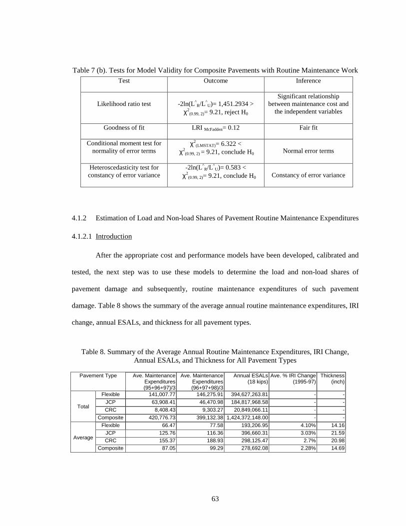
63
Table 7 (b). Tests for Model Validity for Composite Pavements with Routine Maintenance Work Test
Outcome Inference
Likelihood ratio test
-2ln(L^
R/L^U)= 1,451.2934 >
χ2(0.99, 2)= 9.21, reject H0
Significant relationship between maintenance cost and
the independent variables
Goodness of fit
LRI McFadden= 0.12 Fair fit
Conditional moment test for normality of error terms
χ2(LMSTAT)= 6.322 <
χ2(0.99, 2) = 9.21, conclude H0
Normal error terms
Heteroscedasticity test for constancy of error variance
-2ln(L^R/L^
U)= 0.583 < χ2
(0.99, 2)= 9.21, conclude H0
Constancy of error variance
4.1.2 Estimation of Load and Non-load Shares of Pavement Routine Maintenance Expenditures
4.1.2.1 Introduction
After the appropriate cost and performance models have been developed, calibrated and
tested, the next step was to use these models to determine the load and non-load shares of
pavement damage and subsequently, routine maintenance expenditures of such pavement
damage. Table 8 shows the summary of the average annual routine maintenance expenditures, IRI
change, annual ESALs, and thickness for all pavement types.
Table 8. Summary of the Average Annual Routine Maintenance Expenditures, IRI Change, Annual ESALs, and Thickness for All Pavement Types
Pavement Type Ave. Maintenance
Expenditures (95+96+97)/3
Ave. Maintenance Expenditures (96+97+98)/3
Annual ESALs (18 kips)
Ave. % IRI Change (1995-97)
Thickness (inch)
Flexible 141,007.77 146,275.91 394,627,263.81 - -JCP 63,908.41 46,470.98 184,817,968.58 - -CRC 8,408.43 9,303.27 20,849,066.11 - -
Total
Composite 420,776.73 399,132.38 1,424,372,148.00 - -Flexible 66.47 77.58 193,206.95 4.10% 14.16
JCP 125.76 116.36 396,660.31 3.03% 21.59CRC 155.37 188.93 298,125.47 2.7% 20.98
Average
Composite 87.05 99.29 278,692.08 2.28% 14.69

64
4.1.2.2 Analysis of Load Share of Routine Maintenance Expenditures for Flexible, JCP, CRC
and Composite Pavements
(a) Load Share of Routine Maintenance Expenditures for Flexible Pavements
Based on the maintenance expenditure and performance models developed for
flexible pavements, we have
%7.2591.275,146
3375.610,37
3375.610,3781.263,627,394*)1053.9(*
1053.995.206,193
58.77*005158.0*0201.46**)(%
*)(%
1
)(
51)(
5121
11
===
=×=∆∂
∂=
×===∂
∂∂
∂=
∂∂
+
−
−+−
−+++
t
onlyrelatedload
tt
tonlyrelatedload
t
t
t
t
t
t
t
t
ARMETotalARMEExpected
ShareLoad
ESALsAnnualESALsAnnual
ARMEARMEExpected
ESALsAnnualARME
ESALsAnnualChangeIRI
ChangeIRIARME
ESALsAnnualARME
αα
Note: “ARME” refers to the annual routine maintenance expenditures
(b) Load Share of Routine Maintenance Expenditures for JCP Pavements
Based on the maintenance expenditure and performance models developed for
JCP pavements, we have
%7.3598.470,46
1718.16578
1718.578,1658.968,817,184*)1097.8(*
1097.831.660,396
36.116*008105.0*7325.37**
)(%*
)(%
1
)(
51)(
5121
11
===
=×=∆∂
∂=
×===∂
∂∂
∂=
∂∂
+
−
−+−
−+++
t
onlyrelatedload
tt
tonlyrelatedload
t
t
t
t
t
t
t
t
ARMETotalARMEExpected
ShareLoad
ESALsAnnualESALsAnnual
ARMEARMEExpected
ESALsAnnualARME
ESALsAnnualChangeIRI
ChangeIRIARME
ESALsAnnualARME αα
(c) Load Share of Routine Maintenance Expenditures for CRC Pavements
Based on the maintenance expenditure model developed for CRC pavements, we have
%2.6327.303,9
4366.879,5
4366.879,511.066,849,20*)1082.2(*
1082.247.125,298
93.188*4449.0*
1
)(
41)(
411
===
=×=∆∂
∂=
×===∂
∂
+
−
−+−
−++
t
onlyrelatedload
tt
tonlyrelatedload
t
t
t
t
ARMETotalARMEExpected
ShareLoad
ESALsAnnualESALsAnnual
ARMEARMEExpected
ESALsAnnualARME
ESALsAnnualARME α

65
(d) Load Share of Routine Maintenance Expenditures for Composite Pavements
Based on the maintenance expenditure and performance models developed for
composite pavements, we have
%8.2738.132,399
0275.101,111
0275.101,11100.148,372,424,1*)108.7(*
108.708.692,278
1*
10ln1
*0062.0*9762.016,81
*10ln1
**
1
)(
51)(
521
1
===
=×=∆∂
∂=
×===∂
∂
+
−
−+−
−+
t
onlyrelatedload
tt
tonlyrelatedload
tt
t
ARMETotalARMEExpected
ShareLoad
ESALsAnnualESALsAnnual
ARMEARMEExpected
ESALsAnnualESALsAnnualARME
αα
4.1.2.3 Summary of Load Shares of Pavement Routine Maintenance Expenditures for
Flexible, JCP, CRC, and Composite Pavements
Load shares of pavement routine maintenance expenditures for flexible, JCP, CRC, and
composite pavements are summarized in Table 9.
Table 9. Summary of Load Shares of Routine Maintenance Expenditures for Flexible, JCP, CRC and Composite Pavements
Pavement Type Flexible JCP CRC Composite
Load share
(routine maintenance only) 25.7% 35.7% 63.2% 27.8%

66
4.2 Pavement Segments with Rehabilitation Work
In order to estimate the load share of pavement rehabilitation expenditures, it is necessary
to define the service life of a pavement segment, and to obtain reliable measures of pavement
performance over the analysis period. For a pavement segment that has received rehabilitation, its
service life is considered to be the time interval between the last rehabilitation work and the start
of rehabilitation activity that falls in our analysis period (1995 to 1997). For all the pavement
segments for which rehabilitation was commenced in 1996 and 1997, the condition of the
pavement was considered as the terminal condition. This provided a data point with which
extrapolation of roughness trends was carried out. Model development for estimating the load and
non-load shares of pavement rehabilitation expenditures was conducted separately for flexible,
JCP and composite pavements. The general form of the OLS models is shown below:
K
EXPEND(rehab.) = α0 + Σ αi Xi + ε i=1 where
EXPEND(rehab.) = Rehabilitation expenditures;
α’s are model coefficients;
Xi’s are a set of independent variables representing climatic and regional features,
cumulative ESALs, subgrade materials, pavement age, design and construction standards;
and ε’s are error terms.
4.2.1 Model Development for All Pavement Types
This section describes each aspect of the data for each pavement type. SAS software [SAS
Institute, 1996] was used to develop the rehabilitation expenditure models. The calibrated models

67
were then examined for their validity using four standard tests available in the SAS package.
Regression model validity was checked using the following criteria:
• ANOVA hypothesis test;
• Goodness of fit test;
• Correlation test; and
• Modified Levene test.
The ANOVA hypothesis test gives evidence of any relationship between independent
variables and the dependent variable. Goodness of fit test using coefficient of determination
(adjusted R2) showing whether the estimated data points have a good fit with the observed data.
The correlation test was conducted by calculating the coefficient of correlation between the
residuals and their expected values under normality. If the observed coefficient of correlation is at
least as large as the critical value for a given level of significance, it is concluded that the error
terms are reasonably normally distributed. The Modified Levene test is based on the variability of
the residuals. The larger the error variance, the larger the variability of the residuals will tend to
be. To conduct the test, the data set is divided into two groups. Then two sample t-tests based on
the test statistic are carried out to determine whether the mean of the absolute deviations for one
group differs significantly from the mean absolute deviation for the second group. Large absolute
values of t-statistic indicate that the error terms do not have constant variance.

68
4.2.1.1 Model Development for Flexible Pavements
Data from 202 one-mile flexible pavement segments were used for model development.
The descriptive statistics of mean, standard deviation, minimum and maximum values for the
variables initially considered are presented in Appendix 16. As shown in Table 10(a)(i), the
calibrated expenditure model for flexible pavements that received rehabilitation was of the
general form stated in previous section. The significant variables were Cumulative ESALs per
unit thickness (Cumulative ESALs / THICKNESS), interaction term of subgrade materials,
subgrade moisture content and freeze index (P200*MOIST*FZI), drainage coefficient
(DRAINCO) and pavement age (AGE).
The positive sign and high t-statistic value for the cumulative loading per unit thickness
correctly indicates that higher level of traffic loading and smaller pavement thickness are
associated with increased rehabilitation expenditures. Also, clayey subgrade, coupled with a
higher moisture content and a higher freeze index, together constitutes favorable conditions for
increased pavement failure and therefore rehabilitation expenditures. Additionally, the greater the
pavement age, the higher the expenditure for rehabilitation work. The negative sign of the t-
statistic for drainage features indicates that lack of pavement drainage leads to greater levels of
pavement damage.
A summary of test results is given in Table 10(a)(ii). The test results for model validity
provided evidence to the existence of statistically significant relationship between rehabilitation
expenditures and the selected independent variables. Also, the goodness of fit test showed a good
fit, and the correlation test and Modified Levene test indicated that the error terms are normally
distributed and with constant variance.
The model for flexible pavements with rehabilitation and periodic maintenance
expenditures gave similar results for only rehabilitation work. The model coefficients and test

69
results were presented in Tables 10(b)(i) and 10(b)(ii). In both cases, the models did not
implicitly include expenditures for routine maintenance activities carried out during the life cycle
of the pavements.
Table 10 (a)(i). Model Calibration for Flexible Pavements with Rehabilitation Work
Properties
Variable
Value of Coefficient
t-Statistic
Constant Term
172,431 5.4454
Cumulative ESALs
THICKNESS
0.3113
50.6584
P200*MOIST*FZI
300.83 5.4255
DRAINCO
-145,378 -4.6671
(AGE-10)*DM DM is a dummy variable (1 for pavement age≥ 10,
0 otherwise)
701.19
3.3759
Table 10 (a)(ii). Tests for Model Validity for Flexible Pavements with Rehabilitation Work
Test
Outcome Inference
ANOVA hypothesis
From ANOVA table,
P-value = 0.0001< 0.01, reject H0
Significant relationship between rehabilitation cost
and the independent variables
Goodness of fit
Adjusted R2 = 0.96
Good fit
Correlation test for
normality of error terms
Correlation coefficient r=0.984>0.98 (critical value),
conclude H0
Normal error terms
Modified Levene test for constancy of error variance
Levene P-value = 0.13175 > 0.01, conclude H0
Constancy of error variance

70
Table 10(b)(i). Model Calibration for Flexible Pavements with Rehabilitation and Periodic Maintenance Work
Properties
Variable
Value of Coefficient
t-Statistic
Constant Term
170,305 5.3898
Cumulative ESALs THICKNESS
0.3110
50.7293
P200*MOIST*FZI
300.687 5.4348
DRAINCO
-143,243 -4.6086
(AGE-10)*DM DM is a dummy variable (1 for pavement age≥ 10,
0 otherwise)
700.426
3.3796
Table 10(b)(ii). Tests for Model Validity for Flexible Pavements with Rehabilitation and Periodic Maintenance Work
Test
Outcome Inference
ANOVA hypothesis
From ANOVA table,
P-value = 0.0001< 0.01, reject H0
Significant relationship between rehabilitation
cost and the independent variables
Goodness of fit
Adjusted R2 = 0.96
Good fit
Correlation test for normality of error terms
Correlation coefficient r=0.984>0.98 (critical value),
conclude H0
Normal error terms
Modified Levene test for
constancy of error variance
Levene P-value = 0.12563 > 0.01, conclude H0
Constancy of error
variance

71
4.2.1.2 Model Calibration for Jointed Concrete Pavements (JCP)
For the development of rehabilitation expenditure models for JCP pavements, data from
49 one-mile segments were used. The descriptive statistics of variables initially considered are
presented in Appendix 19. As presented in Table 11(a)(i), the significant variables for the
rehabilitation expenditure model were cumulative traffic loading (Cumulative ESALs), JCP slab
thickness (SLABTH), number of days with 320C or more and pavement age.
For JCP pavements with rehabilitation, it was found that traffic loading, number of hot
days with 320C or more and age had direct and significant relationship with pavement
rehabilitation expenditures. This is intuitive. Higher traffic loading, excessive temperatures and
older pavements are expected to result in higher levels of rehabilitation expenditures. The sign of
the coefficient for concrete slab thickness was found to be negative. Again, this is reasonable.
Higher pavement thickness means greater resistance to failure and consequently, less
rehabilitation expenditures.
The test results for model validation were summarized in Table 11(a)(ii). These tests
showed that there was a statistically strong relationship between rehabilitation expenditures of
JCP pavements with the four explanatory variables indicated above, and a good fit was obtained.
Also, the assumptions of normality and constant variance of the error terms were found to be true.
Similar model and test results were obtained for JCP segments that received both periodic
maintenance and rehabilitation as shown in Tables 11(b)(i) and 11(b)(ii).

72
Table 11(a)(i). Model Calibration for JCP Pavement with Rehabilitation Work
Properties
Variable
Value of Coefficient
t-Statistic
Constant Term
-628,986 -3.0901
Cumulative ESALs
0.038 12.5278
SLABTH
-40,020.6 -3.6617
DAYS> 320C
13,274.1 3.7592
AGE
34,759.9 3.9709
Table 11(a)(ii). Tests for Model Validity for JCP Pavement with Rehabilitation Work
Test
Outcome Inference
ANOVA hypothesis
From ANOVA table,
P-value = 0.0001< 0.01, Reject H0
Significant relationship between rehabilitation cost
and the independent variables
Goodness of fit
Adjusted R2 = 0.96 Good fit
Correlation test for normality of error terms
Correlation coefficient r=0.9473>0.94(critical value),
conclude H0
Normal error terms
Modified Levene test for
constancy of error variance
Levene P-value = 0.08 > 0.01, conclude H0
Constancy of error variance

73
Table 11(b)(i). Model Calibration for JCP Pavements with Rehabilitation and Periodic Maintenance Work
Properties
Variable
Value of Coefficient
t-Statistic
Constant Term
-665,863 -3.4230
Cumulative ESALs
0.0374 12.9107
SLABTH
-38,797.5 -3.7144
DAYS> 320C
13,409.3 3.9737
AGE
37,613.1 4.4961
Table 11(b)(ii). Tests for Model Validity for JCP Pavements with Rehabilitation and Periodic Maintenance Work
Test
Outcome Inference
ANOVA hypothesis
From ANOVA table,
P-value = 0.0001< 0.01, Reject H0
Significant relationship between rehabilitation cost
and the independent variables
Goodness of fit
Adjusted R2 = 0.96 Good fit
Correlation test for normality of error terms
Correlation coefficient r=0.9513>0.94(critical value),
conclude H0
Normal error terms
Modified Levene test for
constancy of error variance
Levene P-value = 0.063 > 0.01, conclude H0
Constancy of error variance

74
4.2.1.3 Model Development for Composite Pavements
621 one-mile composite pavement segments provided data for model development. The
descriptive statistics of mean, standard deviation, minimum and maximum values for variables
initially considered are presented in Appendix 22. From Table 12(a)(i), it is seen that the
cumulative traffic loading per unit thickness of composite pavements (Cumulative ESALs /
THICKNESS), product of subgrade moisture and freeze index (MOIST*FZI), minimum
temperature (MINTEM) and pavement age (AGE) were variables found to have direct and
significant impacts on rehabilitation expenditures for composite pavements. This is an expected
inference, because higher levels of pavement loading/thickness ratio, greater levels of moisture
content in subgrade soil, higher freeze levels and pavement age all contribute significantly to
increased pavement deterioration and thus pavement rehabilitation expenditures. The sign of the
coefficient for minimum temperature was found to be negative. This is reasonable. Given other
factors equal, higher minimum temperature provides a better whether condition, relatively less
pavement damage and consequently, lower rehabilitation expenditures.
Table 12(a)(ii) summarized the test results for model validation, the ANOVA hypothesis
test, which typically examines the existence of significant relationship between a dependent
variable and multiple independent variables, indicated that composite pavement rehabilitation
expenditures were strongly dependent on the identified independent variables. The goodness of fit
test showed that the model provided a good fit to the data. Furthermore, the Modified Levene test
showed that the error terms have constant variance. As shown in Tables 12(b)(i) and 12(b)(ii),
similar model and test results were obtained for composite segments that received both periodic
maintenance and rehabilitation.

75
Table 12(a)(i). Model Calibration for Cost Model for Composite Pavements with Rehabilitation Work
Properties
Variable
Value of Coefficient
t-Statistic
Constant Term
540,918 7.4095
Cumulative ESALs THICKNESS
0.2409
29.3913
MOIST*FZI
71.0328 39.5450
MINTEM
-10,392.8 -6.8227
(AGE-10)*DM DM is a dummy variable (1 for pavement age≥ 10,
0 otherwise)
10,593.2
8.8256
Table 12(a)(ii). Tests for Model Validity for Composite Pavements with Rehabilitation Work
Test
Outcome Inference
ANOVA hypothesis
From ANOVA table,
P-value = 0.0001< 0.01, reject H0
Significant relationship between rehabilitation cost
and the independent variables
Goodness of fit
Adjusted R2 = 0.899 Good fit
Correlation test for normality of error terms
Correlation coefficient r=0.95< 0.97(critical value)
Residue plot shows that error terms are normally
distributed
Modified Levene test for constancy of error
variance
Levene P-value = 0.362
> 0.01, conclude H0
Constancy of error variance

76
Table 12(b)(i). Model Calibration for Cost Model for Composite Pavements with Rehabilitation and Periodic Maintenance Work
Properties
Variable
Value of Coefficient
t-Statistic
Constant Term
448,354 5.7782
Cumulative ESALs
THICKNESS
0.2327
26.7081
MOIST*FZI
71.0545 37.2170
MINTEM
-8,337.28 -5.1495
(AGE-10)*DM DM is a dummy variable (1 for pavement age≥ 10,
0 otherwise)
8,961.62
7.0246
Table 12(b)(ii). Tests for Model Validity for Composite Pavements with Rehabilitation and Periodic Maintenance Work
Test
Outcome Inference
ANOVA hypothesis
From ANOVA table, P-value = 0.0001< 0.01,
Reject H0
Significant relationship between rehabilitation cost
and the independent variables
Goodness of fit
Adjusted R2 = 0.885 Good fit
Correlation test for normality of error terms
Correlation coefficient r=0.941< 0.97(critical value)
Residue plot shows that error terms are normally distributed
Modified Levene test for
constancy of error variance
Levene P-value = 0.16752
> 0.01, conclude H0
Constancy of error variance

77
4.2.2 Estimation of Load and Non-load Shares of Pavement Rehabilitation Expenditures
4.2.2.1 Introduction
After the required expenditure models have been developed, the next step was to use
these models to determine the load and non-load shares of pavement damage and subsequently,
cost of rehabilitation of such pavement damage. Table 13 shows the summary of the
rehabilitation /and periodic maintenance expenditures, IRI change, cumulative ESALs, and
thickness for all pavement types.
Table 13. Summary of Capital Costs, IRI Change, Cumulative ESALs, and Thickness for Pavement Segments with Work Commenced in 1996 and 1997
Pavement Type
Rehabilitation (97$)
Rehab. & Periodic Main.
(97$)
Cumulative ESALs
(18 kips)
Thickness
(inch) Flexible 64,581,572.73 64,590,919.00 795,747,416.33 -
JCP 54,097,100.48 54,142,150.01 1,119,342,543.19 -
Total Composite 248,424,282.36 250,946,494.49 4,679,865,437.28 - Flexible 186,890.83 186,916.89 2,197,968.69 13.76
JCP 461,637.03 461,859.62 9,469,896.86 22.04
Average
Composite 247,224.06 249,926.57 4,121,405.48 14.12
4.2.2.2 Analysis of Load Share of Rehabilitation /and Periodic Maintenance Expenditures for
Flexible, JCP and Composite Pavements
(a) Load Shares of Rehabilitation /and Periodic Maintenance Expenditures for Flexible Pavements
(i) Based on Rehabilitation Expenditures
%8.2773.572,581,6468.628,002,18
68.628,002,1833.416,747,795*022623546.0*
022623546.076.13
3113.0
.)(
.)(
.)(.)(
.)(
===
==∆∂
∂=
===∂
∂
rehab
rehab
rehabrehab
rehab
EXPENDTotalEXPENDExpected
ShareLoad
ESALsCumulativeESALsCumulative
EXPENDEXPENDExpected
THICKNESSESALsCumulativeEXPEND α

78
(ii) Based on Rehabilitation and Periodic Maintenance Expenditures
%8.2700.919,590,6454.279,985,17
54.279,985,1733.416,747,795*022601744.0*
022601744.076.13
3110.0
.)&.(
.)&.(
.)&.(.)&.(
.)&.(
===
==∆∂
∂=
===∂
∂
mainperiodicrehab
mainperiodicrehab
mainperiodicrehabmainperiodicrehab
mainperiodicrehab
EXPENDTotalEXPENDExpected
ShareLoad
ESALsCumulativeESALsCumulative
COSTEXPENDExpected
THICKNESSESALsCumulativeEXPEND α
(b) Load Share of Rehabilitation /and Periodic Maintenance Expenditures
for JCP Pavements
(i) Based on Rehabilitation Expenditures
%6.7848.100,097,5463.016,535,42
63.016,535,4219.543,342,119,1*038.0*
038.0
.)(
.)(
.)(.)(
.)(
===
==∆∂
∂=
==∂
∂
rehab
rehab
rehabrehab
rehab
EXPENDTotalEXPENDExpected
ShareLoad
ESALsCumulativeESALsCumulative
EXPENDEXPENDExpected
ESALsCumulativeEXPEND
α
(ii) Based on Rehabilitation and Periodic Maintenance Expenditures
%3.7701.150,142,5411.411,863,41
11.411,863,4119.543,342,119,1*0374.0*
0374.0
.)&.(
.)&.(
.)&.(.)&.(
.)&.(
===
==∆∂
∂=
==∂
∂
mainperiodicrehab
mainperiodicrehab
mainperiodicrehabmainperiodicrehab
mainperiodicrehab
COSTTotalCOSTExpected
ShareLoad
ESALsCumulativeESALsCumulative
COSTCOSTExpected
ESALsCumulativeCOST
α

79
(c) Load Share of Load Share of Rehabilitation /and Periodic Maintenance Expenditures
for Composite Pavements
(i) Based on Rehabilitation Expenditures
%3836.282,424,248
74.308,597,93
74.308,597,9328.437,865,679,4*02.0*
02.012.14
2409.0
.)(
.)(
.)(.)(
.)(
===
==∆∂
∂=
===∂
∂
rehab
rehab
rehabrehab
rehab
COSTTotalCOSTExpected
ShareLoad
ESALsCumulativeESALsCumulative
COSTCOSTExpected
THICKNESSESALsCumulativeCOST α
(ii) Based on Rehabilitation and Periodic Maintenance Expenditures
%3849.494,946,250
74.308,597,93
74.308,597,9328.437,865,679,4*02.0*
02.012.14
2327.0
.)&.(
.)&.(
.)&.(.)&.(
.)&.(
===
==∆∂
∂=
===∂
∂
mainperiodicrehab
mainperiodicrehab
mainperiodicrehabmainperiodicrehab
mainperiodicrehab
COSTTotalCOSTExpected
ShareLoad
ESALsCumulativeESALsCumulative
COSTCOSTExpected
THICKNESSESALsCumulativeCOST α
4.2.2.3 Summary of Load Shares of Rehabilitation /and Periodic Maintenance Expenditures for
Flexible, JCP and Composite Pavements
Load shares of rehabilitation and periodic maintenance expenditures for flexible, JCP and
composite pavements are summarized in Table 14.
Table 14. Summary of Load Shares of Rehabilitation /and Periodic Maintenance Expenditures for
Flexible, JCP and Composite Pavements
Pavement Type Flexible JCP Composite Load Share
Rehabilitation 27.8% 78.6% 38.0% Rehab. & Periodic Maintenance 27.8% 77.3% 38.0%

80
4.3 Chapter Summary
Different approaches were used to establish the load share of pavement damage for
pavement segments that had received maintenance and those that had received rehabilitation. The
development of models that relate maintenance expenditures and pavement condition, and
pavement condition and traffic loading, were readily established Tobit models. However, for
rehabilitation expenditures and traffic loading ordinary least square (OLS) models were used. The
Tobit model, which is described as censored regression model, was used for modeling routine
maintenance expenditures because annual routine maintenance levels are censored by budgetary
constraints. Econometric theory states that in such cases, OLS is not appropriate and censored
regression models yield more consistent estimates.
The rate of change in pavement roughness was found to be a useful response variable for
modeling the influence of traffic, environmental factors as well as pavement age on pavement
damage and maintenance/ rehabilitation expenditures. Both Tobit and OLS models revealed that
load shares of maintenance and rehabilitation expenditures for flexible and composite pavements
were lower than those for rigid pavements. Moreover, for the same type of pavement, the portion
of load share for rehabilitation expenditures was higher than that calculated according to the
maintenance expenditures. This result is as expected because rehabilitation and periodic
maintenance provide added structural capacity.

81
CHAPTER 5 SUMMARY, CONCLUSIONS AND RECOMMENDATIONS
5.1 Summary of Findings
This study utilized a comprehensive database that contains a wide range of data types
relevant to highway pavement performance and expenditures in the State of Indiana. This was
accompanied by definition of appropriate measures of pavement maintenance and rehabilitation,
and pavement condition. Also, the various load and non-load related factors of pavement
deterioration were defined. Three pavement types were considered, and the study period, which
was constrained by data availability and reliability, ranged from 1995 to 1997.
Tobit models were used to explain the variation of routine maintenance expenditures in
response to various load and non-load factors of pavement deterioration, while OLS models were
employed to develop a function relating costs of pavement rehabilitation to pavement
deterioration. From these models, the load shares of pavement maintenance and rehabilitation
expenditures for each pavement type and under each category of pavement repair was
determined.
In order to draw useful conclusions from the results of the current study, it was necessary
to synthesize the findings in four ways:
• Findings by repair category
• Findings by pavement type
• Findings by approach used
• Findings by year of study

82
5.1.1 Findings by Repair Category For each pavement type, repair category consists of routine maintenance, rehabilitation,
and a combination of periodic maintenance and rehabilitation. As periodic maintenance is
relatively very little, interpretation of the study results has been carried out mainly using routine
maintenance and rehabilitation, respectively. For each of these pavement repair categories, the
distribution of load and non-load shares for each pavement type was assessed to determine how
load shares varied across pavement types for that repair category, and attempts were made to
explain the reasons for any observed trends. It was found that regardless of repair category, non-
load effects account for greater repair expenditures for flexible pavements, but that share
diminishes in the case of composite, JCP, and CRC pavements.
5.1.1.1 Findings for Pavements That Had Received Only Routine Maintenance Figure 10 shows the distribution of load and non-load shares of routine maintenance
expenditures for all four-pavement types. This figure shows that the load share of routine
maintenance expenditures is lowest for flexible pavements (about 26%), increases to 28% and
36% for composite and JCP pavements respectively, and is greatest for CRC pavements (63%).
From this it is inferred that the cost of repairing load-related damage to flexible pavements is less
than that for repairing non-load damage on such pavement. This is an important consideration for
any cost allocation study. A possible explanation for this inference is that the interaction effects
of materials used for flexible pavement construction and environmental factors are more
pronounced than for materials and traffic loading. The results further suggest that as pavement
composition is more and more dominated by reinforced concrete and steel content, the load share
of pavement damage increases, and the pavement becomes relatively less vulnerable to non-load
factors of pavement deterioration such as the environment.

83
0%
20%
40%
60%
80%
100%
Relative Share
Flexible JCP CRC Composite
Pavement type
Load and Non-load Shares of Pavement Maintenance Costs
Load Share Non-load Share
Figure 10. Load and Non-load Shares of Pavement Routine Maintenance Expenditures
(Current Study)
0%20%40%60%80%
100%
Relative Share
Flexible JCP Composite
Pavement Type
Load and Non-load Shares of Pavement Rehabilitation Expenditures
Load Share Non-load Share
Figure 11. Load and Non-load Shares of Pavement Rehabilitation Expenditures
(Current Study)
5.1.1.2 Findings for Pavements That Had Undergone Rehabilitation
As shown in Figure 11, of the three pavement types that had undergone rehabilitation,
flexible pavements had the lowest load share of pavement rehabilitation expenditures (28%),
while JCP pavements had the highest share (78%). This suggests that rehabilitation of flexible
pavements, though a structural activity, corrects pavement damage a greater share of which is
induced by environment and other non-load related factors. On the other hand, a greater share of

84
damage on JCP pavements that are repaired by rehabilitation is caused by traffic loading. The
situation for composite pavements is somewhat in between, at 38%. This result is intuitive
because most of composite pavements in Indiana consist of flexible overlays on rigid pavements.
5.1.2 Findings by Pavement Type
It was necessary to analyze the results for each pavement type, so that differences in load
and non-load shares for each repair category applied to the given pavement type can be explained
without bias to pavement materials. An interesting observation is that across all pavement types,
load shares were smaller for sections that had received only routine maintenance than it was for
sections that had received rehabilitation. This result is not unexpected, because routine
maintenance is generally carried out by highway agencies in response to functional defects, while
rehabilitation is done to correct structural deficiencies and to restore load-bearing capacity. A
discussion for each pavement type is presented below.
5.1.2.1 Flexible Pavements
Figure 12(a), the load share of flexible pavement repair expenditures is substantially
lower than non-load share, regardless of repair category. The load share is about 26% for routine
maintenance and is only slightly higher (28%) for rehabilitation. While the higher load share for
rehabilitation is reasonable within the context of intended objective of repair (structural versus
functional), the closeness of the two values reflects the fact that the load share of flexible
pavement repair is not sensitive to repair category.

85
0%
20%
40%
60%
80%
100%
Relative Share
Routine Maintenance Rehabilitation Rehab. and PeriodicMaint.
Repair Category
a. Load and Non-load Shares of Repair Expenditures for Flexible Pavements
Load Share Non-load Share
0%
20%
40%
60%
80%
100%
Relative Share
Routine Maintenance Rehabilitation Rehab. and PeriodicMaint.
Repair Category
b. Load and Non-load Shares of Repair Expenditures for JCP Pavements
Load Share Non-load Share
0%20%40%60%80%
100%
Relative Share
RoutineMaintenance
Rehabilitation Rehab. and PeriodicMaint.
Repair Category
Load and Non-load Shares of Repair Costs for Composite Pavements
Load Share Non-load Share
Figure 12. Load and Non-load Shares of Repair Expenditures for Various Pavement Types

86
5.1.2.2 JCP Pavements
As illustrated in Figure 12(b), the load share of JCP pavement repair expenditures is very
sensitive to repair category. For routine maintenance, only 36% of pavement damage repair is
attributable to load, while for rehabilitation, 78% is attributable to load. This finding suggests that
for JCP pavement repair activities that involve structural capacity improvement, the load share of
repair be over twice the load share for activities that do not improve structural capacity. Therefore
it would be unfair to allocate JCP pavement repair expenditures without due cognizance to the
type of pavement repair.
5.1.2.3 Composite Pavements
Figure 12(c) shows that the load share of composite pavement repair expenditures is not
very sensitive to repair category, as the range of values is 28-38% for routine maintenance and
rehabilitation respectively. The higher load share for rehabilitation compared to that for routine
maintenance is defensible given the fact that routine maintenance activities are mostly carried out
to correct non-structural defects.
5.1.3 Findings by Approach Used
Table 15 shows the comparison of the results of using the current approach and the 1984
Indiana Highway Cost Allocation approach using current data (1995-1997). This table, as well as
Figure 12, shows the distribution of load and non-load shares across pavement types and
pavement repair categories.
As seen from Table 15 and Figure 13, the results obtained in the current study was
generally consistent with those using the 1984 Indiana HCAS approach, with a few exceptions
where differences in results can be considered significant. Both studies found that the impact of

87
load-related factors on pavement repair expenditures was higher for rigid pavements compared to
that for
Table 15. Comparison of Results between Current Study and 1984 Indiana HCAS Approaches
Current Approach 1984 HCAS Approach
Pavement
Type
Repair Type
Repair Details
Load Non-load Load Non-load
Pavement with maintenance
Models based only on routine maintenance
26%
(74%)*3
21%
(79%)
Models based on rehabilitation only
28%
(72%)
Flexible
Pavement with rehabilitation Models based on
rehabilitation and periodic maintenance
28%
(72%)
42%
(58%)
Pavement with maintenance
Models based only on routine maintenance
36%
(64%)
54%
(46%)
Models based on rehabilitation only
79%
(21%)
JCP
Pavement with rehabilitation Models based on
rehabilitation and periodic maintenance
78%
(22%)
85%
(15%)
CRC*1
Pavement with maintenance
Models based only on routine maintenance
63%
(37%)
100%*2
(0)
Pavement with maintenance
Models based only on routine maintenance
28%
(72%)
29%
(71%)
Models based on rehabilitation only
38%
(62%)
Composite
Pavement with rehabilitation Models based on
rehabilitation and periodic maintenance
38%
(62%)
56%
(44%)
Note: 1) For CRC pavement, no analysis was conducted for segments with rehabilitation due to
lack of data.
2) For CRC pavement, only one route was used when conducting analysis by using earlier
Indiana approach. The result may not be representative of all pavement types in
this category.
3) Numbers in parenthesis indicate non-load shares.

88
01020304050
Load Share (%)
1 2Repair Category and
Approach 1- Routine Maintenance
Comparison of Load Shares between Current and 1984 Indiana HCAS Approaches for Flexible
Pavements
Current Approach
1984 IndianaHCAS Approach
020406080
100
Load Share (%)
1 2Repair Category and
Approach 1- Routine Maintenance
Comparison of Load Shares between Current and 1984 Indiana HCAS Approaches for JCP Pavements
Current Approach
1984 IndianaHCAS Approach
0102030405060
Load Share (%)
1 2Repair Category and
Approach 1- Routine Maintenance
Comparison of Load Shares between Current and 1984 Indiana HCAS Approaches for Composite
Pavements
Current Approach
1984 IndianaHCAS Approach
Figure 13. Comparison of Load and Non-load Shares of Pavement Repair Expenditures
2 Rehabilitation
2 Rehabilitation
2 Rehabilitation

89
flexible and composite pavements. A summary of the results obtained using the 1984 Indiana
HCAS approach on the basis of current data set was provided in Appendix 24.
For flexible pavement sections that had received only routine maintenance, the 1984
Indiana HCAS approach found that approximately 21% of damage is attributed to pure load
factor. This was quite similar to the results obtained from the current study (26%). From the
standpoint of rehabilitation and periodic maintenance, the 1984 Indiana HCAS approach found
that 42% of flexible pavement damage is due to pure load factor while the current study found
this value to be 28%. As expected, both studies attribute to flexible pavements with rehabilitation
a greater share of load share of pavement repair expenditures as compared to flexible pavements
with routine maintenance. This is because rehabilitation activities are generally carried out by
highway agencies to address structural deficiencies.
For JCP pavement with maintenance, the 1984 Indiana HCAS approach found that 54%
of pavement damage is due to pure load factors while the current study found that this figure was
in the region of 36%. The value obtained in this study is deemed more realistic because routine
maintenance activities correct only functional deficiencies and do not improve the structural
capacity of the road. Therefore, the load share of pavement repair expenditures from the
standpoint of routine maintenance is expected to be relatively little. The picture for rehabilitated
JCP pavements is similar. The current study finds that for such pavements with rehabilitation,
78% of flexible pavement damage is attributable to load, while the 1984 Indiana HCAS approach
finds that value as 85%.
For CRC pavements, the current study found that about 63% of pavement damage can be
attributed to load-related factors for pavements that had received only routine maintenance. The
1984 Indiana HCAS approach found this value to be 100%, but it is pertinent to note that only

90
one route was used for the analysis in that study, and the result is not expected to be
representative of all routes in that category.
For composite pavements that had received only routine maintenance, the results from
the current study and the 1984 Indiana HCAS approach were somewhat similar, with load shares
of 28% and 29%, respectively. However, for composite pavements that had undergone
rehabilitation, the load share was 38% and 56%, respectively. The difference in these two sets of
values is rather large, and can probably be explained by the difference in the two approaches.
5.1.4 Findings by Year of Study
Finally, a comparison was made on the results of the current approach applied to current
data to the results of the 1984 Indiana HCA approach applied to data at that time. The comparison
revealed differences in the ratio of pavement repair expenditures attributed to load and non-load
factors. The load shares obtained from the current study were consistently lower than those of the
1984 study, for all pavement types. This finding is not unexpected. Over the past 15 years, travel
patterns have changed considerably. Also, vehicle axle configurations, tire pressures, and other
vehicle-related features have also changed. Furthermore, design procedures, material types and
construction techniques have been improved to maximize the structural capacity of a pavement
for a given set of conditions. All these changes have occurred as a result of efforts to improve the
load-bearing capacity of the pavement, increase pavement durability, and to reduce the effective
loading from heavy vehicles.
The obvious reduction in load related effects, coupled with no significant change in non-
load related effects, over the past 15 years, means that the current load shares of repair
expenditures are expected to be lower than those of 15 years ago. The study results are consistent
with this explanation.

91
5.2 Conclusions
It is clear from the current study that the load share of pavement repair expenditures is
highest (over 60%) for CRC pavements, followed by JCP and composite pavements, and is least
for flexible pavements. This is true for all the pavement sections regardless of road repair
category.
Generally, it was revealed that the load shares of pavement repair expenditures for
flexible and composite pavements were lower than those for rigid pavements, regardless of
pavement repair category. Furthermore, for each pavement type, it was found that pavement
sections that had received non-structural pavement repairs (i.e., routine maintenance) had a
relatively smaller load share of repair expenditures as compared to those sections that had
received structure-enhancing repairs (rehabilitation).
Finally, the following conclusions can be made about load shares of pavement repair
expenditures:
• It is sensitive to pavement type
• It is sensitive to pavement repair category
• It is sensitive to the year of study
• For a given pavement type, load share sensitivity differs across pavement repair
categories (most sensitive for JCP, least sensitive for flexible pavements)
In light of the discussion of results, it is imperative that any meaningful and reliable cost
allocation study be preceded by determination of the load and non-load shares of pavement repair
expenditures. This should be carried out with respect to the type of pavements in the network in
question and the various categories of past pavement repair activities, and should utilize, as much
as possible, current data on the network usage, condition and maintenance expenditures.

92
5.3 Recommendations and Directions for Future Work and Research
The observations and results from this study can be salient inputs for the update of the
highway cost allocation study for Indiana. This way, a fair and equitable distribution of highway
costs allocation can be revised to ensure that pavement maintenance and rehabilitation
expenditures are distributed in an equitable and efficient manner. This study can be extended
further to examine the load and non-load shares of expenditures used for different activities of
maintenance, such as pothole patching, resealing, etc. Another area of further study is the implicit
consideration of routine maintenance in the rehabilitation expenditure models.

93
REFERENCES
AASHTO [1976], AASHTO Maintenance Manual, American Association of State Highway and Transportation Officials, Washington, D. C. AASHTO [1993], AASHTO Interim Guide for Design of Pavement Structures, American Association of State Highway and Transportation Officials, Washington, D.C. Al-Suleiman, T., and Sinha, K. C. [1988], “An Evaluation of Effects of Routine Maintenance on Pavement Surface Condition”, School of Civil Engineering, Purdue University, West Lafayette, Indiana. Ben-Akiva, M., Humplick, F., Madanat, S. and Ramaswamy, R. [1992], “Latent Performance Approach to Infrastructure Management”, Transportation Research Record 1311, Transportation Research Board, National Research Council, Washington, D.C. Butler, B. C., Charmichael, R. F., and Flanagan, P. R. [1985], “ Impact of Pavement Maintenance on Damage Rate”, Volume 1, Final Report, ARE, Inc., Consultants, DTFH61-83-C-00125, Federal Highway Administration, Washington, D. C. Econometric Software [1998], “LIMDEP User’s Manual”, Econometric Software, Plainview, New York. Fwa, T. F. and Sinha, K. C. [1986], “Study of the Effects of Routine Pavement Maintenance”, Transportation Research Record 1102, Transportation Research Board, National Research Council, Washington, D.C. Fwa, T. F. and Sinha, K. C. [1987], “Estimation of Environmental and Traffic Loading Effects on Highway Pavements”, Australian Road Research 17(4), Australian Road Research Board Ltd, Victoria, Australia. Goldberger, A. S. [1964], Econometric Theory, New York: John Wiley & Sons, Inc., New York, N.Y. Gopinath, D., Ben-Akiva, M. and Ramaswamy, M. [1996], “Modeling Performance of Highway Pavements”, Transportation Research Record 1449, Transportation Research Board, National Research Council, Washington, D.C. Greene, W. H. [1999], Econometric Analysis, Prentice Hall, Upper Saddle River, New Jersey. Gulen, S., Nagle, J., Zhu, K., MacArthur, S., and Hooker, G. [1998], “Determination of Practical ESALs on Indiana Roads”, Indiana Department of Transportation, Indiana.

94
Hajek, J. J., Tighe, S. L., and Hutchinson, B. G. [1998], “ Allocation of Pavement Damage Due to Truck Using a Marginal Cost Method”, Transportation Research Record 1613, Transportation Research Board, National Research Council, Washington, D. C. Huang, Y. H. [1993], Pavement Analysis and Design, Prentice Hall, Englewood Cliffs, New Jersey. Lytton, R. L. [1988], “Concepts of Pavement Performance Prediction and Modeling”, Department of Civil Engineering, Texas A & M University, College Station, Texas. Mannering, F. L., and Kilareski, W. P. [1998], Principle of Highway Engineering and Traffic Analysis, John Wiley & Sons, Inc., New York, N. Y. Mohammed, D., McCarthy, P. and Sinha, K. C. [1997], “The Mixed Logit Approach”, Transportation Research Record 1597, Transportation Research Board, National Research Council, Washington, D.C. Martin, T. [1994], “Pavement Behavior Prediction for Life-cycle Costing”, Australian Road Research 255, Australian Road Research Board Ltd, Victoria, Australia. Oregon Department of Transportation (Oregon DOT) [1987], “1986 Oregon Highway Cost Allocation Study”, Salem, Oregon. Oregon Department of Transportation (Oregon DOT) [1995], “1994 Oregon Highway Cost Allocation Study”, Salem, Oregon. Paterson, W. D. O. [1987], Road Deterioration and Maintenance Effects: Models for Planning and Management, Johns Hopkins University Press, Baltimore, Maryland. Perera, R. W., Byrum, C., and Kohn, S. D. [1995], “Investigation of Pavement Roughness”, Final Report, Report No. FHWA-RD-97-147, Federal Highway Administration, Washington, D. C. Ramaswamy, R. and Ben-Akiva, M. [1997], “Estimation of Highway Pavement Deterioration from In-Service Pavement Data”, Transportation Research Record 1570, Transportation Research Board, National Research Council, Washington, D.C. Rilett, L. R., Hutchinson, B. G., and Hass R. C. G. [1990], “Cost Allocation Implications of Flexible Pavement Deterioration Models”, Transportation Research Record 1215, Transportation Research Board, National Research Council, Washington, D. C. SAS Institute. [1996], “SAS/INSIGHT User’s Guide”, SAS Institute Inc., Cary, North Carolina. Sinha, K. C., Fwa, T. F., Ting, E. C., Shanteau, R. M., Saito, M. and Michael, H. L. [1984], “Indiana Highway Cost Allocation Study”, School of Civil Engineering, Purdue University, West Lafayette, Indiana. Small, K. A., Winston, C., and Evans, C. [1989], Road Work: A New Highway Pricing and Investment Policy, The Brookings Institution, Washington, D. C.

95
Strategic Highway Research Program (SHRP) [1994], “Evaluation of the AASHTO Design Equations and Recommended Improvements”, Washington, D.C. United States Department of Transportation (U.S. DOT) [1998], “1997 Federal Highway Cost Allocation Study”, Washington, D.C. Virginia Department of Transportation (VIDOT) [1983], “1982 Virginia Highway Cost Allocation Study”, Richmond, Virginia. Whitford, R. K. [1998], “State of Alaska: Truck Weight Monitoring Plan Using Weigh-in-Motion Devices”, Final Report, Project No. 76095, Purdue University, West Lafayette, Indiana. Yoder, E. J. [1975], Principles of Pavement Design, New York: John Wiley & Sons, New York City, New York.

xi
LIST OF ABBREVIATIONS
AADT Average Annual Daily Traffic
AASHO American Association of State Highway Officials
AASHTO American Association of State Highway and Transportation Officials
ANOVA Analysis of Variance
ARE Austin Research Engineers
ARME Annual Routine Maintenance Expenditures
ARRB Australia Road Research Board
CBR California Bearing Ratio
CESALs Cumulative Equivalent Single Axle Loads
CRC Continuously Reinforced Concrete
DI Damage Index
DOT Department of Transportation
DM Dummy Variable
ESALs Equivalent Single Axle Loads
EUAC Equivalent Uniform Annual Cost
FHWA Federal Highway Administration
FZI Freeze Index
FZTHAW Freeze-thaw Cycles
GPS General Pavement Study
HCAS Highway Cost Allocation Study

xii
HMAC Hot Mix Asphalt Concrete
INDOT Indiana Department of Transportation
IPMS Indiana Pavement Management Systems
IRI International Roughness Index
JCP Jointed Concrete Pavement
JPCP Jointed Plain Concrete Pavement
JTRP Joint Transportation Research Program
LEF Load Equivalency Factor
LIMDEP Limited Dependent Variable (Software Package)
LRI Likelihood Ratio Index
LTPP Long Term Pavement Performance
MAXTEM Maximum Temperature
MDI Modified Damage Index
MINTEM Minimum Temperature
NCHRP National Cooperative Highway Research Program
OLS Ordinary Least Square
PCC Portland Cement Concrete
PMS Pavement Management Systems
PSI Present Serviceability Index
RCI Ride Comfort Index
RMSVA Root Mean Square Vertical Acceleration
RN Roughness Number
SAS Statistical Analysis System (Software Package)
SHRP Strategic Highway Research Program
SN Structural Number

xiii
TSI Terminal Serviceability Index
VMT Vehicle Miles of Travel
WIM Weigh-in-Motion
WLEF Weighted Load Equivalency Factor

APPENDICES

96
Appendix 1. Definition of General Model Parameters For Routine Maintenance

97
PARAMETER DEFINITION UNIT 94TFA Expenditures of routine maint. by force account and periodic maint. by contract in 1994 $/lane-mile/year (98$)95TFA Expenditures of routine maint. by force account and periodic maint. by contract in 1995 $/lane-mile/year (98$)96TFA Expenditures of routine maint. by force account and periodic maint. by contract in 1996 $/lane-mile/year (98$)97TFA Expenditures of routine maint. by force account and periodic maint. by contract in 1997 $/lane-mile/year (98$)98TFA Expenditures of routine maint. by force account and periodic maint. by contract in 1998 $/lane-mile/year (98$)94FA Routine maintenance Expenditures only by force account in 1994 $/lane-mile/year (98$)95FA Routine maintenance Expenditures only by force account in 1995 $/lane-mile/year (98$)96FA Routine maintenance Expenditures only by force account in 1996 $/lane-mile/year (98$)97FA Routine maintenance Expenditures only by force account in 1997 $/lane-mile/year (98$)98FA Routine maintenance Expenditures only by force account in 1998 $/lane-mile/year (98$)94IRI IRI measurement in 1994 inch/mile95IRI IRI measurement in 1995 inch/mile96IRI IRI measurement in 1996 inch/mile97IRI IRI measurement in 1997 inch/mile95IRICH % change in IRI between 1994 and 95 96IRICH % change in IRI between 1995 and 96 97IRICH % change in IRI between 1996 and 97 95LIRI1 Log10( % change in IRI between 1994 and 95+100%) 96LIRI1 Log10( % change in IRI between 1995 and 96+100%) 97LIRI1 Log10( % change in IRI between 1996 and 97+100%) IRI0 Initial IRI inch/mileALPHA Predicted annual IRI increment rate inch/mileR2
IRI R2 of the regression model for the extrapolation of initial IRI IRIT Terminal IRI inch/milePSI0 Initial pavement serviceability index PSIT Terminal pavement serviceability index AVE456T Average annual routine and periodic maintenance Expenditures during 1994-96 $/lan-mile/year (98$)AVE567T Average annual routine and periodic maintenance Expenditures during 1995-97 $/lan-mile/year (98$)AVE678T Average annual routine and periodic maintenance Expenditures during 1996-98 $/lan-mile/year (98$)AVE9456 Average annual routine maintenance Expenditures during 1994-96 $/lan-mile/year (98$)AVE9567 Average annual routine maintenance Expenditures during 1995-97 $/lan-mile/year (98$)AVE9678 Average annual routine maintenance Expenditures during 1996-98 $/lan-mile/year (98$)567IRI Average % change in IRI during 1995, 96 and 97 567IRI1 Average % change in IRI during 1995, 96 and 97+100% FZI Freeze index degree-dayFZTHAW Freeze thaw cycle no. of cyclesDAY0SF No. of days between first minimum of 00C between Spring and Fall dayMEANTEM Average annual temperature 0FMAXTEM Maximum annual temperature 0FMINTEM Minimum annual temperature 0FDAY32 No. of days > 320C dayDAY0 No. of days < 00C dayPRECIP Annual precipitation inch/yearLPRE Log10(annual precipitation) WETDAY Annual no. of wet days dayWET Annual no. of wet days dayP200 Subgrade percent passing #200 sieve weight %P200LPR Subgrade percent passing #200 sieve * log10(annual precipitation) weight % * inch/yearMOIST Subgrade moisture content %LL Subgrade liquid limit %PL Subgrade plastic limit %PI Subgrade plasticity index %SUBDEN Maximum dry density of subgrade materials lb/inch3
CBR93 California bearing capacity at 93% %REMOD Subgrade resilient modulus psiLREMOD Log10(subgrade resilient modulus) 95AADT Average annual daily traffic in 1995 vehicle/day96AADT Average annual daily traffic in 1996 vehicle/day97AADT Average annual daily traffic in 1997 vehicle/day95TRUCK Truck percentage in traffic stream in 1995 %96TRUCK Truck percentage in traffic stream in 1996 %97TRUCK Truck percentage in traffic stream in 1997 %95LANE Lane traffic in 1995 vehicle/day96LANE Lane traffic in 1996 vehicle/day

98
97LANE Lane traffic in 1997 vehicle/day567AADT Average of AADT during 1995-97 vehicle/dayAADT2 (Average of AADT during 1995-97-5,000) * alpha1 [alpha1 = 1, if AADT>5,000] vehicle/dayAADT3 (Average of AADT during 1995-97-50,000) * alpha2 [alpha2 = 1, if AADT>50,000] vehicle/day567TRUC Average truck percentage in traffic stream during 1995-97 %567LANE Average lane traffic during 1995-97 vehicle/dayINESAL Equivalent single axle loads computed by INDOT method 18kipsWHESAL Equivalent single axle loads computed by Whitford method 18kips95ESAL Equivalent single axle loads in 1995 computed by Weighted-LEF method 18kips96ESAL Equivalent single axle loads in 1996 computed by Weighted-LEF method 18kips97ESAL Equivalent single axle loads in 1997computed by Weighted-LEF method 18kipsAVEESAL Average equivalent single axle loads during 1995-97 by Weighted-LEF method 18kipsLAVESAL Log10(average equivalent single axle loads during 1995-97) CESAL Cumulative equivalent single axle loads during one life cycle 18kipsLCESAL Log10(cumulative equivalent single axle loads during one life cycle) LESALAB Log10[cumulative equivalent single axle loads /(sub/base + HMAC thickness)] PSIESAL PSI-cumulative ESALs loss during one life cycle 94AGE Pavement age in 1994 year95AGE Pavement age in 1995 year96AGE Pavement age in 1996 year97AGE Pavement age in 1997 yearAGE Pavement age yearAGE2 (Pavement age-5 or 8) * beta1 [beta1 = 1, if age > 5 for flexible or > 8 for rigid) yearAGE3 (Pavement age-10 or 15) * beta2 [beta2 = 1, if age >10 for flexible or >15 for rigid) yearDRAINCO Drainage coefficient BASETH Sub/base thickness inchBLPRE Sub/base thickness * log10(precipitation) inch * (inch/year)BASECOM Sub/base compaction %HMACTH Hot mix asphalt concrete (HMAC) thickness inchSLABTH Slab thickness inchTHICK Sub/base thickness + HMAC thickness or slab thickness inchESAL/TH Equvalent single axle loads / (sub/base + HMAC thickness or slab thickness) 18kips/inchLESALTH Log10[equvalent single axle loads / (sub/base + HMAC thickness or slab thickness)] 18kips/inchAC32 HMAC thickness * no. of days > 320C inch * daySLAB32 Slab thickness * no. of days > 320C inch * dayLACBASE Log10(sub/base thickness + HMAC thickness) LSLBASE Log10(subbase thickness + slab thickness) ASPHCON Asphalt content weight %AGG4 Percent of aggregate in HMAC passing #4 sieve weight %LAGG4 Log10(percent of aggregate in HMAC passing #4 sieve) AIRVOID Air voids in HMAC volume %LAV Log10(air voids in HMAC) D32AV No. of days > 320C * Air voids in HMAC day * volume %ELASMOD Modulus of elasticity of concrete pavement psiRUPMOD Modulus of rupture of concrete pavement psiJOINT Joint spacing between concrete slabs ftDOWEL Diameter of dowel inch

99
Appendix 2. Variables Considered for the Model Development of Flexible Pavements
with Routine Maintenance

100
Equation 1: Tobit Model Dependent Variable UnitAverage annual routine maintenance Expenditures during 1996-98 (in 98 $) $/lane-mile/year Independent Variables Average % change in IRI of flexible pavement during 1995-97 Region: Dummy variables District: Dummy variables Road Type: Dummy variables Pavement Age: Average of 1995-97 yearAge2: Dummy variable (for age group of 6-10 years) Age3: Dummy variable (for age group of 10 years up) Equation 2: Simultaneous Regression Equation Dependent Variable Average % change in IRI of flexible pavement during 1995-97 Independent Variables Average annual routine maintenance Expenditures during 1995-97 (in 98 $) $/lane-mile/yearRegion: Dummy variables District: Dummy variables Road Type: Dummy variables Freeze index degree-dayFreeze-thaw cycle no. of daysNo. of days between last Spring and first Fall of minimum of 00C no. of daysMean annual temperature 0FMaximum annual temperature 0FMinimum annual temperature 0FNo. of days > 320C no. of daysNo. of days < 00C no. of daysAverage annual precipitation inches/yearAverage no. of wet days no. of daysSubgrade % passing #200 sieve weight %Subgrade moisture content %Subgrade plastic index %Maximum dry density of subgrade material psiSubgrade modulus of resilience psiAADT vehicles/dayAADT2: Dummy variable AADT3: Dummy variable % Truck in traffic stream %Lane distribution based on WIM data %Vehicle composition based on WIM data %Vehicle operating weight distribution based on WIM data %ESALs 18 kips

101
Pavement age yearAge2: Dummy variable (for age group of 6-10 years) Age3: Dummy variable (for age group of 10 years up) Drainage coefficient Sub/base thickness inchesBase thickness * precipitation inches2
Base compaction %Hot mix asphalt concrete (HMAC) thickness inchesHMAC thickness * no. of days > 320C inches * daysESALs/ (sub/base thickness + HMAC thickness) 18kips/inchAsphalt content in HMAC %Hot mix asphalt concrete % aggregate < #4 sieve weight %Air voids in hot mix asphalt concrete volume %No. of days > 320C * air voids days * volume %

102
Appendix 3. Descriptive Statistics of All Variables Initially Considered for Flexible Pavement Modeling Based on Routine Maintenance

103
Flexible pavements Mean Std. Deviation Minimum Maximum Unit
AVE9456 63.13 39.40 0.00 911.23 $/lane-mile/year (98$) AVE9567 66.47 39.40 0.00 911.23 $/lane-mile/year (98$) AVE9678 77.58 12.23 0.00 1,736.90 $/lane-mile/year (98$)
567IRI 0.04 0.00 -0.34 0.33 567IRI1 0.02 0.00 -0.18 0.12
FZI 280.49 81.37 74.62 1,483.80 degree-day FZTHAW 95.40 5.19 65.33 115.95 no.of cycles DAY0SF 177.46 1.61 87.88 265.85 day
MEANTEM 51.35 1.45 48.60 54.81 0F MAXTEM 54.66 1.75 52.30 57.82 0F MINTEM 48.13 1.31 46.29 51.98 0F DAY32 23.98 1.41 13.00 49.00 day DAY0 113.35 11.31 96.00 124.00 day
PRECIP 41.01 5.46 7.29 70.93 inch/year LPRE 1.61 0.07 0.86 1.85
WETDAY 117.16 7.78 95.00 134.00 day P200 0.72 0.14 0.14 1.00 weight %
P200LPR 84.31 21.95 18.18 133.46 weight % * inch/year MOIST 0.17 0.06 0.08 0.33 %
PI 12.94 7.35 0.00 38.50 % SUBDEN 108.55 0.00 95.60 136.90 lb/inch3
REMOD 6,164.86 106.07 2,700.00 17,400.00 psi LREMOD 3.77 0.01 3.43 4.24 567AADT 9,016.85 3,340.49 214.21 76,397.33 vehicle/day AADT2 3,992.13 1,605.10 0.00 37,139.00 vehicle/day AADT3 167.88 0.00 0.00 26,397.33 vehicle/day
AVEESAL 193,206.95 52,490.26 482.09 2,961,015.91 18kips LAVESAL 4.77 0.39 2.68 6.47
AGE 10.04 4.95 2.67 25.00 year AGE2 1.25 3.54 0.00 5.00 year AGE3 1.92 0.00 0.00 15.00 year
DRAINCO 1.06 0.07 1.00 1.10 BASETH 12.04 2.12 2.25 20.00 inch BLPRE 19.57 3.51 2.50 45.97 inch * (inch/year)
BASECOM 0.95 0.00 0.95 0.95 HMACTH 2.11 0.18 0.60 16.00 inch
THICK 14.16 2.30 4.70 28.00 inch ESAL/TH 14,826.43 4,844.41 37.81 569,597.18 18kips/inch LESALTH 3.63 0.47 1.58 5.76
AC32 53.96 1.77 8.13 784.00 inch * day LACBASE 1.13 0.07 0.67 1.45 ASPHCON 0.06 0.00 0.06 0.07 weight %
AGG4 0.35 0.00 0.35 0.35 weight % LAGG4 -0.46 0.00 -0.46 -0.46
AIRVOID 0.06 0.00 0.06 0.06 volume % LAV -1.22 0.00 -1.22 -1.22
D32AV 1.44 0.08 0.78 2.94 day * volume %
Note: The detailed explanations of the variables listed above are given in Appendix 1.

104
Appendix 4. Details of Model Validation for Cost and Performance Models Developed for
Flexible Pavements Based on Routine Maintenance

105
Model Validation
(1) Likelihood Ratio Test
Null hypothesis H0: All the ßi = 0 Alternative hypothesis H1: At least one ß ≠ 0 Let L^
U = the Likelihood function of the Tobit model without constraints Let L^
R = the Likelihood function of the Tobit model with constraints From the LIMDEP output, the following is obtained: The null hypothesis is rejected. This means that there is a relationship between the dependent
variable (expected maintenance expenditures) and the dependent variables (pavement condition change, age, and road type).
(2) Goodness of Fit
(3) Conditional Moment Test for Normality Assumption of Error Terms
Null hypothesis H0: The error term is normal Alternative hypothesis H1: The error term is not normal
From LIMDEP output, we have
LMSTAT = .43445396835470370D+01Q = .20000000000000000D+01Result = .88608125423125720D+00
χ2(LMSTAT)=4.3445<χ2
(0.99, 2)=9.21 (critical value) The null hypothesis is not rejected.
(4) Heteroscedasticity Test Null hypothesis H0: The error term is homoscedastic Alternative hypothesis H1: The error term is heteroscedastic From LIMDEP output, the log-likelihood from the original model is -921.4153, and
the log-likelihood from the expanded model is -916.7502
[ ] )(28.13)4,99.0(3302.9)7502.916(4153.921*2ln2 2
exp
valuecriticalanded
original
LL =<=−−−−=
���
�
�
���
�
�
− ∧
∧
χ
Fail to reject null hypothesis. The error term is homoscedastic.
177.0)786.929()9177.764(1
ln
ln1 =
−−−=
���
�
�
���
�
�
−= ∧
∧
R
UMcFadden
LLLRI
)(34.11)3,99.0(7366.329ln*2ln2 2)9177.764(
)786.929(
valuecriticalee
U
R
LL =>>=��
�
����
�−=
���
�
�
���
�
�
− −
−
∧
∧
χ

106
Appendix 5. Variables Considered for the Model Development of JCP Pavements
with Routine Maintenance

107
Equation 1: Tobit Model Dependent Variable Average annual routine maintenance expenditures during 1996-98 (in 98 $) $/lane-mile/year Independent Variables Average % change in IRI of PCC pavement during 1995-97 Region: Dummy variables District: Dummy variables Road Type: Dummy variables Pavement Age: Average of 1995-97 yearAge2: Dummy variable (for age group of 9-15 years) Age3: Dummy variable (for age group of 15 years up) Equation 2: Simultaneous Regression Equation Dependent Variable Average % change in IRI of PCC pavement during 1995-97 Independent Variables Average annual routine maintenance expenditures during 1995-97 (in 98 $) $/lane-mile/yearRegion: Dummy variables District: Dummy variables Road Type: Dummy variables Freeze index degree-dayFreeze-thaw cycle no. of daysNo. of days between last Spring and first Fall of minimum of 00C no. of daysMean annual temperature 0FMaximum annual temperature 0FMinimum annual temperature 0FNo. of days > 320C no. of daysNo. of days < 00C no. of daysAverage annual precipitation inches/yearAverage no. of wet days no. of daysSubgrade % passing #200 sieve weight %Subgrade moisture content %Subgrade plastic index %Maximum dry density of subgrade material psiSubgrade modulus of resilience psiAADT vehicles/dayAADT2: Dummy variable AADT3: Dummy variable % Truck in traffic stream %ESALs 18 kipsPavement age yearAge2: Dummy variable (for age group of 9-15 years) Age3: Dummy variable (for age group of 15 years up) Drainage coefficient

108
Subbase thickness inchesBase thickness * precipitation inches2
Base compaction %Slab thickness inchesSlab thickness * no. of days > 320C inches * daysESALs/ (sub/base thickness + slab thickness) 18kips/inchConcrete modulus of elasticity psiConcrete modulus of rupture psiJoint spacing of concrete pavement feetDiameter of dowels in concrete pavement inches

109
Appendix 6. Descriptive Statistics of All Variables Initially Considered for JCP Pavement Modeling Based on Routine Maintenance

110
JCP pavements Mean Std. Deviation Minimum Maximum Unit
AVE9456 149.75 321.00 0.00 1,611.19 $/lane-mile/year (98$)AVE9567 125.76 121.97 0.00 1,457.27 $/lane-mile/year (98$)AVE9678 116.36 128.44 0.00 1,469.18 $/lane-mile/year (98$)567IRI 0.03 0.08 -0.17 0.16 567IRI1 0.01 0.03 -0.08 0.06 FZI 247.81 38.81 74.68 399.93 degree-dayFZTHAW 85.98 5.79 65.33 114.33 no. of cyclesDAY0SF 180.16 25.62 162.72 255.51 dayMEANTEM 52.01 1.18 48.60 56.05 0FMAXTEM 55.00 1.75 52.30 57.82 0FMINTEM 48.81 3.11 46.58 52.38 0FDAY32 26.62 15.56 13.00 49.00 dayDAY0 111.37 13.44 96.00 124.00 dayPRECIP 41.35 11.10 23.13 84.13 inch/yearLPRE 1.61 0.16 1.36 1.92 WETDAYS 115.91 7.07 95.00 134.00 dayP200 0.74 0.07 0.25 1.00 weight %P200LPRE 84.85 13.03 31.62 124.00 MOIST 0.17 0.05 0.11 0.24 %PI 12.31 1.34 2.00 32.00 %SUBDEN 108.88 9.62 94.10 127.43 lb/inch3
REMOD 6,580.85 1,909.19 2,100.00 12,300.00 psiLREMOD 3.79 0.19 3.32 4.09 567AADT 22,463.08 16,155.61 960.14 126,067.28 vehicle/dayAADT2 8,532.98 16,155.61 0.00 37,239.26 vehicle/dayAADT3 4,361.40 0.00 0.00 76,067.28 vehicle/dayAVEESALs 396,660.31 712,845.37 9,876.44 4,448,972.89 18kipsLAVESAL 5.23 0.59 3.99 6.65 AGE 14.29 8.01 5.33 29.00 yearAGE2 2.12 0.00 0.00 6.00 yearAGE3 2.24 2.36 0.00 14.00 yearDRAINCO 1.08 0.00 1.00 1.10 BASETH 11.52 5.66 1.00 20.00 inchBASELPRE 18.71 7.56 1.59 33.17 BASECOM 0.95 0.00 0.95 0.95 %SLABTH 10.07 3.54 0.60 16.00 inchTHICK 21.59 2.12 5.50 36.00 inchESAL/TH 20,710.51 38,177.91 456.72 222,448.64 18kips/inchLESALTH 3.93 0.57 2.66 5.35 SLAB32 299.55 94.05 8.13 784.00 inch * dayLSLBASE 1.30 0.06 0.74 1.56 ELASMOD 3,990,543.74 0.00 2,666,666.67 4,000,000.00 psiRUPMOD 660.93 0.00 441.67 662.50 psiJOINT 19.95 0.00 13.33 20.00 ftDOWEL 1.20 0.18 0.00 1.50 inch
Note: The detailed explanations of the variables listed above are given in Appendix 1.

111
Appendix 7. Details of Model Validation for Cost and Performance Models Developed for
JCP Pavements Based on Routine Maintenance

112
Model Validation
(1) Likelihood Ratio Test Null hypothesis H0: All the ßi = 0 Alternative hypothesis H1: At least one ß ≠ 0 Let L^
U = the Likelihood function of the Tobit model without constraints Let L^
R = the Likelihood function of the Tobit model with constraints From the LIMPED output, the following is obtained:
)(21.9)2,99.0(6604.20ln*2ln2 2)2590.166(
)5892.176(
valuecriticalee
U
R
LL =>=��
�
����
�−=
���
�
�
���
�
�
− −
−
∧
∧
χ
The null hypothesis is rejected. There is relationship between the dependent variable (expected maintenance expenditures) and the dependent variables (pavement condition change and region).
(2) Goodness of Fit
(3) Conditional Moment Test for Normality Assumption of Error Terms From LIMDEP output, we have
LMSTAT = .11627380972778710D+01Q = .20000000000000000D+01Result = .44086763662819650D+00
χ2(LMSTAT)=1.163 < χ2
(0.99, 2) = 9.21 (critical value)
The hypothesis of normality is not rejected.
(4) Heteroscedasticity Test Null hypothesis H0: The error term is homoscedastic Alternative hypothesis H1: The error term is heteroscedastic From LIMPED output, the log-likelihood from the original model is -189.3097, and
the log-likelihood from the expanded model is -184.7047
[ ] )(21.9)2,99.0(2096.9)7047.184(3097.189*2ln2 2
exp
valuecriticalanded
original
LL =<=−−−−=
���
�
�
���
�
�
− ∧
∧
χ
Fail to reject null hypothesis. The error term is homoscedastic.
06.0)5892.176()2590.166(1
ln
ln1 =
−−−=
���
�
�
���
�
�
−= ∧
∧
R
UMcFadden
LLLRI

113
Appendix 8. Variables Considered for the Model Development of CRC Pavements
with Routine Maintenance

114
Tobit Model Dependent Variable Average annual routine maintenance expenditures during 1996-98 (in 98 $) $/lane-mile/year Independent Variables Average annual routine maintenance expenditures during 1995-97 (in 98 $) $/lane-mile/yearAverage % change in IRI of CRC pavement during 1995-97 Region: Dummy variables District: Dummy variables Road Type: Dummy variables Freeze index degree-dayFreeze-thaw cycle no. of daysNo. of days between last Spring and first Fall of minimum of 00C no. of daysMean annual temperature 0FMaximum annual temperature 0FMinimum annual temperature 0FNo. of days > 320C no. of daysNo. of days < 00C no. of daysAverage annual precipitation inches/yearAverage no. of wet days no. of daysSubgrade % passing #200 sieve weight %Subgrade moisture content %Subgrade plastic index %Maximum dry density of subgrade material psiSubgrade modulus of resilience psiAADT vehicles/dayAADT2: Dummy variable AADT3: Dummy variable % Truck in traffic stream %ESALs 18 kipsPavement age yearAge2: Dummy variable (for age group of 9-15 years) Age3: Dummy variable (for age group of 15 years up) Drainage coefficient Subbase thickness inchesBase thickness * precipitation inches2
Base compaction %Slab thickness inchesSlab thickness * no. of days > 320C inches * daysESALs/ (sub/base thickness + slab thickness) 18kips/inchConcrete modulus of elasticity psiConcrete modulus of rupture psiJoint spacing of concrete pavement feet

115
Appendix 9. Descriptive Statistics of All Variables Initially Considered for CRC Pavement Modeling Based on Routine Maintenance

116
CRC pavements Mean Std. Deviation Minimum Maximum Unit
AVE9456 108.08 215.52 0.00 813.75 $/lane-mile/year (98$)AVE9567 155.37 371.48 0.00 1,457.27 $/lane-mile/year (98$)AVE9678 188.93 386.01 0.00 1,469.18 $/lane-mile/year (98$)567IRI 0.03 0.03 0.00 0.11 567IRI1 0.01 0.01 0.00 0.05 FZI 168.92 82.96 108.74 399.93 degree-dayFZTHAW 74.66 12.63 65.33 99.00 no. of cyclesDAY0SF 174.23 1.63 171.89 177.00 dayMEANTEM 52.84 1.50 49.79 53.95 0FMAXTEM 56.40 1.94 52.30 57.82 0FMINTEM 49.85 1.50 46.58 50.97 0FDAY32 29.31 10.07 13.00 37.00 dayDAY0 114.97 6.06 104.00 124.00 dayPRECIP 44.72 4.24 38.16 47.95 inch/yearLPRE 1.65 0.04 1.58 1.68 WETDAYS 116.69 5.73 113.00 134.00 dayP200 0.83 0.16 0.49 0.99 weight %P200LPRE 96.77 18.70 62.38 122.39 MOIST 0.19 0.01 0.17 0.21 %PI 15.95 9.88 4.50 37.70 %SUBDEN 104.64 2.45 99.90 109.10 lb/inch3
REMOD 6,191.38 1,858.81 4,050.00 11,400.00 psiLREMOD 3.78 0.11 3.61 4.06 567AADT 22,864.95 18,324.54 3,367.63 83,800.91 vehicle/dayAADT2 12,542.98 7,724.41 0.00 28,404.60 vehicle/dayAADT3 2,331.10 8,716.60 0.00 33,800.91 vehicle/dayAVEESALs 298,125.47 500,388.96 27,052.64 1,658,345.35 18kipsLAVESAL 5.03 0.57 4.43 6.22 AGE 16.90 8.64 3.00 24.00 yearAGE2 0.21 0.62 0.00 2.00 yearAGE3 5.21 4.16 0.00 9.00 yearDRAINCO 1.03 0.05 1.00 1.10 BASETH 13.62 2.40 8.00 16.00 inchBASELPRE 22.47 4.05 12.65 26.89 BASECOM 0.95 0.00 0.95 0.95 %SLABTH 7.36 2.86 1.00 11.00 inchTHICK 20.98 3.63 12.00 24.00 inchESAL/TH 15,327.25 27,059.83 1,978.93 99,747.69 18kips/inchLESALTH 3.71 0.58 3.30 5.00 SLAB32 224.26 117.18 15.00 407.00 inch * dayLSLBASE 1.31 0.09 1.08 1.38 ELASMOD 4,000,000.00 0.00 4,000,000.00 4,000,000.00 psiRUPMOD 662.50 0.00 662.50 662.50 psiJOINT 20.00 0.00 20.00 20.00 ftDOWEL 1.17 0.42 0.00 1.50 inch
Note: The detailed explanations of the variables listed above are given in Appendix 1.

117
Appendix 10. Details of Model Validation for Cost Model Developed for CRC Pavements
Based on Routine Maintenance

118
Model Validation (1) Likelihood Ratio Test
Null hypothesis H0: All the ßi = 0 Alternative hypothesis H1: At least one ß ≠ 0 Let L^
U = the Likelihood function of the Tobit model without constraints Let L^
R = the Likelihood function of the Tobit model with constraints From the LIMPED output, the following is obtained:
)(21.9)2,99.0(6682.23ln*2ln2 2)1458.18(
)9799.29((
valuecriticalee
U
R
LL =>=��
�
����
�−=
���
�
�
���
�
�
− −
−
∧
∧
χ
The null hypothesis is rejected. There is relationship between the dependent variable (expected maintenance expenditures) and the dependent variables (pavement condition change and region).
(2) Goodness of Fit
(3) Conditional Moment Test for Normality Assumption of Error Terms
From LIMDEP output, we have LMSTAT = .19429845215490040D+01Q = .20000000000000000D+01Result = .62148222367106650D+00
χ2(LMSTAT )= 1.943 < χ2
(0.99, 2) = 9.21 (critical value)
The hypothesis of normality is not rejected. (4) Heteroscedasticity Test
Null hypothesis H0: The error term is homoscedastic Alternative hypothesis H1: The error term is heteroscedastic From LIMPED output, the log-likelihood from the original model is -20.2308, and
the log-likelihood from the expanded model is -16.2438
[ ] )(21.9)2,99.0(974.7)2438.16(2308.20*2ln2 2
exp
valuecriticalanded
original
LL =<=−−−−=
���
�
�
���
�
�
− ∧
∧
χ
Fail to reject null hypothesis. The error term is homoscedastic.
39.0)9799.29()1458.18(1
ln
ln1 =
−−−=
���
�
�
���
�
�
−= ∧
∧
R
UMcFadden
LLLRI

119
Appendix 11. Variables Considered for the Model Development of Composite Pavements
With Routine Maintenance

120
Tobit Model Dependent Variable Average annual routine maintenance expenditures during 1996-98 (in 98 $) $/lane-mile/yearIndependent Variables Average annual routine maintenance expenditures during 1995-97 (in 98 $) $/lane-mile/yearAverage % change in IRI of overlay pavement during 1995-97 Region: Dummy variables District: Dummy variables Road Type: Dummy variables Freeze index degree-dayFreeze-thaw cycle no. of daysNo. of days between last Spring and first Fall of minimum of 00C no. of daysMean annual temperature 0FMaximum annual temperature 0FMinimum annual temperature 0FNo. of days > 320C no. of daysNo. of days < 00C no. of daysAverage annual precipitation inches/yearAverage no. of wet days no. of daysSubgrade % passing #200 sieve weight %Subgrade moisture content %Subgrade plastic index %Maximum dry density of subgrade material psiSubgrade modulus of resilience psiAADT vehicles/dayAADT2: Dummy variable AADT3: Dummy variable % Truck in traffic stream %Lane distribution based on WIM data %Vehicle composition based on WIM data %Vehicle operating weight distribution based on WIM data %ESALs 18 kipsPavement age yearAge2: Dummy variable (for age group of 6-10 years) Age3: Dummy variable (for age group of 10 years up) Drainage coefficient Sub/base thickness inchesBase thickness * precipitation inches2
Base compaction %Hot mix asphalt concrete (HMAC) thickness inchesHMAC thickness * no. of days > 320C inches * daysESALs/ (sub/base thickness + HMAC thickness) 18kips/inchAsphalt content in HMAC %Hot mix asphalt concrete % aggregate < #4 sieve weight %Air voids in hot mix asphalt concrete volume %

121
Appendix 12. Descriptive Statistics of All Variables Initially Considered for Composite Pavement Modeling Based on Routine Maintenance

122
Composite pavements Mean Std. Deviation Minimum Maximum Unit
AVE9456 91.49 211.47 0.00 1,708.66 $/lane-mile/year (98$)AVE9567 87.05 187.66 0.00 1,457.27 $/lane-mile/year (98$)AVE9678 99.29 247.94 0.00 1,736.90 $/lane-mile/year (98$)567IRI 0.02 0.06 -0.34 0.30 567IRI1 0.01 0.03 -0.18 0.11 FZI 296.22 108.26 74.68 851.54 degree-dayFZTHAW 89.92 8.67 49.32 116.06 no. of cyclesDAY0SF 175.22 7.75 111.26 240.43 dayMEANTEM 50.85 1.50 46.99 55.38 0FMAXTEM 54.00 1.54 49.54 57.82 0FMINTEM 47.79 1.37 44.01 54.66 0FDAY32 19.23 8.05 13.00 49.00 dayDAY0 113.97 7.97 96.00 124.00 dayPRECIP 41.95 7.97 17.97 89.33 inch/yearLPRE 1.62 0.07 1.25 1.95 WETDAYS 122.07 8.85 95.00 134.00 dayP200 0.70 0.20 0.10 1.00 weight %P200LPRE 85.59 24.93 12.06 133.73 weight % * inch/yearMOIST 0.37 2.87 0.08 47.10 %PI 14.44 10.97 1.90 125.10 %SUBDEN 109.48 12.57 1.60 139.70 lb/inch3
REMOD 6,374.58 2,094.02 0.00 22,050.00 psiLREMOD 3.80 3.32 0.00 4.34 567AADT 13,873.01 17,997.50 886.83 179,319.88 vehicle/dayAADT2 6,569.00 8,972.63 0.00 41,307.28 vehicle/dayAADT3 1,362.80 9,331.92 0.00 129,319.88 vehicle/dayAVEESALs 278,692.08 589,834.54 1,807.61 6,445,080.17 18kipsLAVESAL 4.98 0.65 3.26 6.81 AGE 8.59 3.62 1.67 25.00 yearAGE2 1.80 1.83 0.00 5.33 yearAGE3 0.83 2.12 0.00 15.00 yearDRAINCO 1.25 2.90 1.00 51.36 BASETH 12.21 3.49 2.50 21.00 inchBASELPRE 19.73 5.71 3.91 33.66 inch * (inch/year)BASECOM 0.95 0.00 0.95 1.00 HMACTH 2.49 2.14 0.27 16.00 inchTHICK 14.69 3.48 5.00 28.00 inchESAL/TH 24,005.09 64,678.70 112.98 745,302.83 18kips/inchLESALTH 3.83 0.68 2.05 5.87 AC32 47.75 63.66 4.05 784.00 inch * dayLACBASE 1.15 0.12 0.70 1.45 ASPHCON 0.06 0.02 0.06 0.36 weight %AGG4 0.35 0.11 0.35 2.23 weight %LAGG4 -0.46 0.05 -0.46 0.35 AIRVOID 0.06 0.00 0.06 0.06 volume %LAV -1.22 0.00 -1.22 -1.22 D32AV 1.15 0.48 0.78 2.94 day * volume %

123
Appendix 13. Details of Model Validation for Cost and Performance Models Developed for
Composite Pavements Based on Routine Maintenance

124
Model Validation (1) Likelihood Ratio Test
Null hypothesis H0: All the ßi = 0 Alternative hypothesis H1: At least one ß ≠ 0 Let L^
U = the Likelihood function of the Tobit model without constraints Let L^
R = the Likelihood function of the Tobit model with constraints From the LIMPED output, the following is obtained:
)(21.9)2,99.0(2934.451,1ln*2ln2 2)4208.593,13(
)1274.142,12(
valuecriticalee
U
R
LL =>=��
�
����
�−=
���
�
�
���
�
�
− −
−
∧
∧
χ
The null hypothesis is rejected. There is relationship between the dependent variable (expected maintenance expenditures) and the dependent variables (pavement condition change and region).
(2) Goodness of Fit
(3) Conditional Moment Test for Normality Assumption of Error Terms
From LIMDEP output, we have LMSTAT = .63221116743408670D+01
Q = .20000000000000000D+01 Result = .95761902992717200D+00
χ2(LMSTAT) = 6.322 < χ2
(0.99, 2) = 9.21 (critical value)
The hypothesis of normality is not rejected. (4) Heteroscedasticity Test
Null hypothesis H0: The error term is homoscedastic Alternative hypothesis H1: The error term is heteroscedastic From LIMPED output, the log-likelihood from the original model is -9,960.216, and
the log-likelihood from the expanded model is -9,959.633
[ ] )(21.9)2,99.0(583.0)9,959.633(9,960.216*2ln2 2
exp
valuecritical
anded
original
LL =<=−−−−=
���
�
�
���
�
�
− ∧
∧
χ
Fail to reject null hypothesis. The error term is homoscedastic.
12.0)4208.593,13()1274.142,12(1
ln
ln1 =
−−−=
���
�
�
���
�
�
−= ∧
∧
R
UMcFadden
LLLRI

125
Appendix 14. Definition of General Modeling Parameters for Rehabilitation

126
PARAMETER DEFINITION UNIT 94RCON Expenditures of rehabilitation for pavement segment with contract awarded in 1994 $/lane-mile (97$)95RCON Expenditures of rehabilitation for pavement segment with contract awarded in 1995 $/lane-mile (97$)96RCON Expenditures of rehabilitation for pavement segment with contract awarded in 1996 $/lane-mile (97$)97RCON Expenditures of rehabilitation for pavement segment with contract awarded in 1997 $/lane-mile (97$)98RCON Expenditures of rehabilitation for pavement segment with contract awarded in 1998 $/lane-mile (97$)94CON Expenditures of rehab. and periodic main. for pavement segment with contract awarded in 1994 $/lane-mile (97$)95CON Expenditures of rehab. and periodic main. for pavement segment with contract awarded in 1995 $/lane-mile (97$)96CON Expenditures of rehab. and periodic main. for pavement segment with contract awarded in 1996 $/lane-mile (97$)97CON Expenditures of rehab. and periodic main. for pavement segment with contract awarded in 1997 $/lane-mile (97$)98CON Expenditures of rehab. and periodic main. for pavement segment with contract awarded in 1998 $/lane-mile (97$)94IRI IRI measurement in 1994 inch/mile95IRI IRI measurement in 1995 inch/mile96IRI IRI measurement in 1996 inch/mile97IRI IRI measurement in 1997 inch/mile96IRICH % change between initial and terminal IRI for segment rehabilitated in 1996 96LIRI1 Log10(% change between initial and terminal IRI for segment rehabilitated in 1996+ 100%) 97IRICH % change between initial and terminal IRI for segment rehabilitated in 1997 97LIRI1 Log10(% change between initial and terminal IRI for segment rehabilitated in 1997+ 100%) IRI0 Initial IRI inch/mileALPHA Predicted annual IRI increment rate inch/mileRIRI R2 of the regression model for the extrapolation of initial IRI IRIT Terminal IRI inch/milePSI0 Initial pavement serviceability index PSIT Terminal pavement serviceability index FZI Average freeze index during one life cycle degree-dayFZTHAW Average freeze thaw cycle during one life cycle no.DAY0SF Average no. of days of first minimum of 00C between Spring and Fall during one life cycle dayMEANTEM Average annual temperature during one life cycle 0FMAXTEM Average maximum annual temperature during one life cycle 0FMINTEM Average minimum annual temperature during one life cycle 0FDAY32 Average no. of days > 320C during one life cycle dayDAY0 Average no. of days < 00C during one life cycle dayPRECIP Average annual precipitation during one life cycle inch/yearLPRE Log10(average annual precipitation during one life cycle) WETDAY Average annual no. of wet days during one life cycle dayP200 Subgrade percent passing #200 sieve weight %P200LPRE Subgrade percent passing #200 sieve * log10(annual precipitation) MOIST Subgrade moisture content %LL Subgrade liquid limit %PL Subgrade plastic limit %PI Subgrade plasticity index %SUBDEN Maximum dry density of subgrade materials lb/inch3
CBR93 California bearing capacity at 93% REMOD Subgrade resilient modulus psiLREMOD Log10(subgrade resilient modulus) 96AADT AADT in 1996 vehicle/day96LANE Lane traffic in 1996 vehicle/day96TRUCK Truck percentage in traffic stream in 1996 %97AADT AADT in 1997 vehicle/dayAADT2 (AADT - 5,000) * alpha1 [alpha1 = 1, if AADT>5,000] vehicle/dayAADT3 (AADT - 50,000) * alpha2 [alpha2 = 1, if AADT>50,000] vehicle/day97LANE Lane traffic in 1997 vehicle/day97TRUCK Truck percentage in traffic stream in 1997 %INESALs Equivalent single axle loads computed by INDOT method 18kipsWHESALs Equivalent single axle loads computed by Whitford method 18kips96ESALs Equivalent single axle loads in 1996 computed by Weighted-LEF method 18kipsAVEESALs Average equivalent single axle loads during 1995-97 computed by Weighted-LEF method 18kipsCESALs Cumulative ESALs during one life cycle computed by Weighted-LEF method 18kipsLCESALS Log10(cumulative ESALs during one life cycle computed by Weighted-LEF method) 18kipsLESALAB Log10[cumulative ESALs during one life cycle/(sub/base+HMAC or slab thickness)] PSIESAL PSI-cumulative ESALs loss during one life cycle 96AGE Pavement age in 1996 year97AGE Pavement age in 1997 year

127
AGE2 (Pavement age-5 or 8) * beta1 [beta1 = 1, if age > 5 for flexible or > 8 for rigid) yearAGE3 (Pavement age-10 or 15) * beta2 [beta2 = 1, if age >10 for flexible or >15 for rigid) yearDRAINCO Drainage coefficient BASETH Sub/base thickness inchBASELPRE Sub/base thickness * log10(average annual precipitation during on life cycle) inch * (inch/year)BASECOM Sub/base compaction %HMACTH Hot mix asphalt concrete (HMAC) thickness inchSLABTH Concrete slab thickness THICK Sub/base thickness + HMAC or slab thickness inchCESAL/TH Cumulative ESALs during one life cycle / (sub/base + HMAC or slab thickness) 18kips/inchLESALTH Log10[cumulative ESALs during one life cycle / (sub/base + HMAC or slab thickness)] AC32 HMAC thickness * no. of days > 320C inch * daySLAB32 Slab thickness * no. of days > 320C inch * dayLACBASE Log10(sub/base thickness + HMAC thickness) LSLBASE Log10(sub/base thickness + slab thickness) ASPHCON Asphalt content weight %AGG4 Percent of aggregate in HMAC passing #4 sieve weight %LP4 Log10(percent of aggregate in HMAC passing #4 sieve) AIRVOID Air voids in HMAC volume %LAV Log10(air voids in HMAC) D32AV No. of days > 320C * Air voids in HMAC day * volume %ELASMOD Modulus of elasticity of concrete pavement psiRUPMOD Modulus of rupture of concrete pavement psiJOINT Joint spacing between concrete slabs footDOWEL Diameter of dowel inch

128
Appendix 15. Variables Considered for the Model Development of Flexible Pavements
with Rehabilitation work

129
Regression Model Dependent Variable Rehabilitation Expenditures required for the flexible pavements after one service life (in 97 $)
$/lane-mile
Independent Variables Region: Dummy variables District: Dummy variables Road Type: Dummy variables % change in IRI of the flexible pavements during one life cycle Average freeze index during one life cycle degree-dayAverage freeze-thaw cycle during one life cycle no. of daysAverage no. of days between last Spring and first Fall of minimum of 00C during one life cycle
no. of days
Average mean annual temperature during one life cycle 0FAverage maximum annual temperature during one life cycle 0FAverage minimum annual temperature during one life cycle 0FAverage no. of days > 320C during one life cycle no. of daysAverage no. of days < 00C during one life cycle no. of daysAverage annual precipitation during one life cycle inches/yearAverage no. of wet days during one life cycle no. of daysSubgrade % passing #200 sieve weight %Subgrade moisture content %Subgrade plastic index %Maximum dry density of subgrade material psiSubgrade modulus of resilience psiAADT vehicles/dayAADT2: Dummy variable AADT3: Dummy variable % Truck in traffic stream %Lane distribution based on WIM data %Vehicle composition based on WIM data %Vehicle operating weight distribution based on WIM data %ESALs 18 kipsPavement age yearAge2: Dummy variable (for age group of 6-10 years) Age3: Dummy variable (for age group of 10 years up) Drainage coefficient Sub/base thickness inchesBase thickness * precipitation inches2
Base compaction %Hot mix asphalt concrete (HMAC) thickness inchesHMAC thickness * no. of days > 320C inches * daysESALs/ (sub/base thickness + HMAC thickness) 18kips/inchAsphalt content in HMAC %Hot mix asphalt concrete % aggregate < #4 sieve weight %Air voids in hot mix asphalt concrete volume %No. of days > 320C * air voids days * volume %

130
Appendix 16. Descriptive Statistics of All Variables Initially Considered for Flexible Pavement Modeling Based on Rehabilitation and Periodic Maintenance

131
Flexible pavements Mean Std deviation Minimum Maximum Unit 96RCON 151,807.21 291,605.22 0.00 1,347,963.64 $/lane-mile (97$)97RCON 35,083.61 75,286.04 0.00 378,189.50 $/lane-mile (97$)96CON 151,807.21 291,605.22 0.00 1,347,963.64 $/lane-mile (97$)97CON 35,122.90 75,280.60 0.00 378,189.50 $/lane-mile (97$)IRICH 1.40 3.72 0.01 45.50 LIRI1 0.27 0.25 0.00 1.67 IRI0 78.38 32.40 3.00 233.63 IRIT 140.14 48.65 56.18 242.82 FZI 197.12 127.37 54.28 494.30 degree-dayFZTHAW 95.22 11.59 74.00 127.00 no. of cyclesDAY0SF 178.15 7.42 165.00 192.75 dayMEANTEM 52.48 2.44 48.30 55.49 0FMAXTEM 55.25 2.81 49.20 58.77 0FMINTEM 49.14 1.44 46.70 51.74 0FDAY32 28.93 11.55 13.00 49.00 dayDAY0 108.16 9.02 96.00 124.00 dayPRECIP 41.92 3.34 35.05 46.25 inch/yearLPRE 1.62 0.04 1.54 1.67 WETDAY 115.80 11.55 95.00 134.00 dayP200 0.73 0.21 0.16 1.00 weight %P200LPRE 1.18 0.35 0.26 1.65 MOIST 0.17 0.03 0.08 0.22 %PI 12.92 7.64 3.00 32.00 %REMOD 6,585.89 2,081.35 2,850.00 12,000.00 psiLREMOD 3.80 0.14 3.45 4.08 AADT 7,513.99 9,187.26 507.32 49,181.73 vehicle/dayAADT2 4,110.49 8,230.40 0.00 44,181.73 vehicle/dayAADT3 0.00 0.00 0.00 0.00 vehicle/dayCESALs 2,197,968.69 5,937,541.35 14,871.49 44,119,137.13 18kipsLCESALS 5.46 0.85 4.17 7.64 AGE 12.34 5.43 3.00 27.00 ageAGE2 0.83 1.63 0.00 5.00 ageAGE3 3.26 4.44 0.00 17.00 ageDRAINCO 1.04 0.05 1.00 1.10 BASETH 11.29 3.35 2.30 17.00 inch/yearBASELPRE 18.27 5.32 3.55 27.47 BASECOM 0.95 0.00 0.95 0.95 %HMACTH 2.46 2.40 0.60 16.00 inch/yearTHICK 13.76 3.72 4.70 22.00 inch/yearCESAL/TH 202,955.62 755,071.63 929.47 6,388,975.52 18kips/inchLESALTH 4.34 0.87 2.97 6.81 AC32 82.94 116.72 10.00 784.00 inch * dayASPHCON 0.06 0.00 0.06 0.07 weight %AGG4 0.35 0.00 0.35 0.35 weight %LP4 -0.46 0.00 -0.46 -0.46 AIRVOID 0.06 0.00 0.06 0.06 volume %LAV -1.22 0.00 -1.22 -1.22 D32AV 1.74 0.69 0.78 2.94 day * volume %
Note: The detailed explanations of the variables listed above are given in Appendix 14.

132
Appendix 17. Details of Model Validation for Cost Models Developed for Flexible Pavements
Based on Rehabilitation /and Periodic Maintenance

133
I. Details of cost model developed for flexible pavements based on rehabilitation
Model Validation
(1) ANOVA Hypothesis Test
H0: EXPEND and Cumulative ESALs, THICKNESS, P200, MOIST, FZI,
DRAINCO and AGE are linearly independent
H1: EXPEND and Cumulative ESALs, THICKNESS, P200, MOIST, FZI,
DRAINCO and AGE are linearly dependent
From the SAS/INSIGHT ANOVA table, we get a P-value=0.0001< 0.01. Therefore,
there is enough evidence from the data, to conclude that EXPEND and Cumulative
ESALs, THICKNESS, P200, MOIST, FZI, DRAINCO and AGE are linearly related.
(2) Goodness of Fit
Based on SAS output, the adjust R2= 0.9666, which indicates a good fit of the model.
(3) Correlation Test for Normality of the Error Term
H0: If correlation coefficient r> critical value at level of significance 0.01, the
distribution of error term is normal
H1: If correlation coefficient r< critical value at level of significance 0.01, the
distribution of error term is not normal
From the SAS/INSIGHT ANOVA table, we get correlation coefficient
r=√(SSR/SST)= √(3.797/3.924)=0.984>0.982 (critical value). Therefore, the
assumption of normally distributed error term is satisfied.
(4) Modified Levene Test for Constant Variance of the Error Term
H0: The error term variances are constant
H1: The error term variances are nonconstant
The Levene SAS program from the EXPEND data gives a P-value of 0.13175.
Since the P-value= 0.13175 > 0.01, there is not enough evidence to reject the null
hypothesis of constant variances. Therefore, the assumption of constant variance of
the error term is not violated.

134
II. Details of cost model developed for flexible pavements based on rehabilitation and periodic maintenance
Model Validation
(1) ANOVA Hypothesis Test H0: EXPEND and Cumulative ESALs, THICKNESS, P200, MOIST, FZI,
DRAINCO and AGE are linearly independent H1: EXPEND and Cumulative ESALs, THICKNESS, P200, MOIST, FZI,
DRAINCO and AGE are linearly dependent From the SAS/INSIGHT ANOVA table, we get a P-value=0.0001< 0.01. Therefore, there is enough evidence from the data, to conclude that EXPEND and Cumulative ESALs, THICKNESS, P200, MOIST, FZI, DRAINCO and AGE are linearly related.
(2) Goodness of Fit Based on SAS output, the adjust R2= 0.9668, which indicates a good fit of the model.
(3) Correlation Test for Normality of the Error Term H0: If correlation coefficient r> critical value at level of significance 0.01, the
distribution of error term is normal H1: If correlation coefficient r< critical value at level of significance 0.01, the
distribution of error term is not normal From the SAS/INSIGHT ANOVA table, we get correlation coefficient r=√(SSR/SST)= √(3.797/3.923)=0.984>0.982 (critical value). Therefore, the assumption of normally distributed error term is satisfied.
(4) Modified Levene Test for Constant Variance of the Error Term H0: The error term variances are constant H1: The error term variances are nonconstant The Levene SAS program from the EXPEND data gives a P-value of 0.12563. Since the P-value= 0.12563 > 0.01, there is not enough evidence to reject the null hypothesis of constant variances. Therefore, the assumption of constant variance of the error term is not violated.
Note: EXPEND = Rehabilitation /and Periodic Maintenance Expenditures

135
Appendix 18. Variables Considered for the Model Development of JCP pavements
with Rehabilitation Work

136
Regression Model Dependent Variable Rehabilitation expenditures required for PCC pavements after one service life (in 97 $)
$/lane-mile
Independent Variables Region: Dummy variables District: Dummy variables Road Type: Dummy variables % change in IRI of the PCC pavements during one life cycle Average freeze index during one life cycle degree-dayAverage freeze-thaw cycle during one life cycle no. of daysAverage no. of days between last Spring and first Fall of minimum of 00C during one life cycle
no. of days
Average mean annual temperature during one life cycle 0FAverage maximum annual temperature during one life cycle 0FAverage minimum annual temperature during one life cycle 0FAverage no. of days > 320C during one life cycle no. of daysAverage no. of days < 00C during one life cycle no. of daysAverage annual precipitation during one life cycle inches/yearAverage no. of wet days during one life cycle no. of daysSubgrade % passing #200 sieve weight %Subgrade moisture content %Subgrade plastic index %Maximum dry density of subgrade material psiSubgrade modulus of resilience psiAADT vehicles/dayAADT2: Dummy variable AADT3: Dummy variable % Truck in traffic stream %ESALs 18 kipsPavement age yearAge2: Dummy variable Age3: Dummy variables Drainage coefficient Subbase thickness inchesBase thickness * precipitation inches2
Base compaction %Slab thickness inchesSlab thickness * no. of days > 320C inches * daysESALs/ (sub/base thickness + slab thickness) 18kips/inchConcrete modulus of elasticity psiConcrete modulus of rupture psiJoint spacing of concrete pavement feetDiameter of dowels in concrete pavement inches

137
Appendix 19. Descriptive Statistics of All Variables Initially Considered for JCP Pavement Modeling Based on Rehabilitation and Periodic Maintenance

138
JCP pavements Mean Std. Deviation Minimum Maximum Unit 96RCON 391,881.21 613,734.42 0.00 2,471,043.33 $/lane-mile (97$)97RCON 69,755.82 231,082.08 0.00 1,234,118.07 $/lane-mile (97$)96CON 397,977.69 610,056.29 0.00 2,471,043.33 $/lane-mile (97$)97CON 69,892.87 231,053.82 0.00 1,234,118.07 $/lane-mile (97$)IRICH 0.62 1.36 0.00 7.46 LIRI1 0.14 0.20 0.00 0.93 IRI0 98.60 48.23 7.88 208.50 IRIT 128.55 54.33 55.44 229.63 FZI 151.12 72.50 54.28 325.50 degree-dayFZTHAW 88.78 11.72 74.00 127.00 no. of cyclesDAY0SF 179.40 6.82 167.00 192.75 dayMEANTEM 53.37 1.56 50.20 55.49 0FMAXTEM 55.85 1.88 52.10 58.77 0FMINTEM 49.71 1.21 46.91 51.74 0FDAY32 31.76 11.88 16.00 49.00 dayDAY0 108.69 11.54 96.00 124.00 dayPRECIP 43.14 2.71 35.05 46.25 inch/yearLPRE 1.63 0.03 1.54 1.67 WETDAY 115.82 12.60 95.00 128.00 dayP200 0.74 0.23 0.25 1.00 weight %P200LPRE 1.21 0.38 0.39 1.65 MOIST 0.18 0.03 0.10 0.24 %PI 13.15 4.66 2.90 26.00 %REMOD 6,716.33 2,542.50 2,100.00 12,300.00 psiLREMOD 3.80 0.17 3.32 4.09 AADT 26,015.45 34,495.02 1,756.52 119,040.00 vehicle/dayAADT2 5,967.51 8,486.34 0.00 35,265.18 vehicle/dayAADT3 8,056.94 19,680.01 0.00 69,040.00 vehicle/dayCESALs 18,939,793.71 42,326,065.19 243,724.97 169,060,969.84 18kipsLCESALS 6.54 0.79 5.39 8.23 AGE 11.43 5.89 4.00 22.00 ageAGE2 1.10 2.04 0.00 6.00 ageAGE3 1.10 1.98 0.00 7.00 ageDRAINCO 1.09 0.02 1.00 1.10 BASETH 13.31 4.68 2.50 20.00 inch/yearBASELPRE 21.82 7.82 3.96 33.30 BASECOM 0.95 0.00 0.95 0.95 %SLABTH 8.73 3.45 0.63 14.00 inch/yearTHICK 22.04 6.25 5.50 30.00 inch/yearCESAL/TH 908,640.70 2,066,465.45 9,026.85 8,453,048.49 18kips/inchLESALTH 5.22 0.80 3.96 6.93 ELASMOD 4,000,000.00 0.00 4,000,000.00 4,000,000.00 psiRUPMOD 662.50 0.00 662.50 662.50 psiDOWEL 1.17 0.54 0.00 1.50 inch
Note: The detailed explanations of the variables listed above are given in Appendix 14.

139
Appendix 20. Details of Model Validation for Cost Models Developed for JCP Pavements
Based on Rehabilitation /and Periodic Maintenance

140
I. Details of cost model developed for JCP pavements based on rehabilitation
Model Validation
(1) ANOVA Hypothesis Test H0: EXPEND and Cumulative ESALs, SLABTH, DAY32 and AGE are linearly
independent H1: EXPEND and Cumulative ESALs, SLABTH, DAY32 and AGE are linearly
dependent From the SAS/INSIGHT ANOVA table, we get a P-value=0.0001< 0.01. Therefore, there is enough evidence from the data, to conclude that EXPEND and Cumulative ESALs, SLABTH, DAY32 and AGE are linearly related.
(2) Goodness of Fit Based on SAS output, the adjust R2= 0.8823 which indicates a good fit of the model.
(3) Correlation Test for Normality of the Error Term H0: If correlation coefficient r> critical value at level of significance 0.01, the
distribution of error term is normal H1: If correlation coefficient r< critical value at level of significance 0.01, the
distribution of error term is not normal From the SAS/INSIGHT ANOVA table, we get correlation coefficient r=√(SSR/SST)= √(1.024/1.141=0.9473 >0.947 (critical value). Therefore, the assumption of normally distributed error term is satisfied.
(4) Modified Levene Test for Constant Variance of the Error Term H0: The error term variances are constant H1: The error term variances are nonconstant The Levene SAS program from the EXPEND data gives a P-value of 0.078824. Since the P-value = 0.078824 > 0.01, there is not enough evidence to reject the null hypothesis of constant variances. Therefore, the assumption of constant variance of the error term is not violated.

141
II. Details of cost model developed for JCP pavements based on rehabilitation and periodic
maintenance
Model Validation
(1) ANOVA Hypothesis Test H0: EXPEND and Cumulative ESALs, SLABTH, DAY32 and AGE are linearly
independent H1: EXPEND and Cumulative ESALs, SLABTH, DAY32 and AGE are linearly
dependent From the SAS/INSIGHT ANOVA table, we get a P-value=0.0001< 0.01. Therefore, there is enough evidence from the data, to conclude that EXPEND and Cumulative ESALs, SLABTH, DAY32 and AGE are linearly related.
(2) Goodness of Fit Based on SAS output, the adjust R2= 0.8911, which indicates a good fit of the model.
(3) Correlation Test for Normality of the Error Term H0: If correlation coefficient r> critical value at level of significance 0.01, the
distribution of error term is normal H1: If correlation coefficient r< critical value at level of significance 0.01, the
distribution of error term is not normal From the SAS/INSIGHT ANOVA table, we get correlation coefficient r=√(SSR/SST)= √(1.019/1.126=0.9513 >0.947 (critical value). Therefore, the assumption of normally distributed error term is satisfied.
(4) Modified Levene Test for Constant Variance of the Error Term H0: The error term variances are constant H1: The error term variances are nonconstant The Levene SAS program from the EXPEND data gives a P-value of 0.062801. Since the P-value = 0.062801 > 0.01, there is not enough evidence to reject the null hypothesis of constant variances. Therefore, the assumption of constant variance of the error term is not violated.
Note:
EXPEND = Rehabilitation /and Periodic Maintenance Expenditures

142
Appendix 21. Variables Considered for the Model Development of Composite Pavements
with Rehabilitation Work

143
Regression Model Dependent Variable Rehabilitation expenditures required for composite pavements after one service life (in 97 $)
$/lane-mile
Independent Variables Region: Dummy variables District: Dummy variables Road Type: Dummy variables % change in IRI of the composite pavements during one life cycle Average freeze index during one life cycle degree-dayAverage freeze-thaw cycle during one life cycle no. of daysAverage no. of days between last Spring and first Fall of minimum of 00C during one life cycle
no. of days
Average mean annual temperature during one life cycle 0FAverage maximum annual temperature during one life cycle 0FAverage minimum annual temperature during one life cycle 0FAverage no. of days > 320C during one life cycle no. of daysAverage no. of days < 00C during one life cycle no. of daysAverage annual precipitation during one life cycle inches/yearAverage no. of wet days during one life cycle no. of daysSubgrade % passing #200 sieve weight %Subgrade moisture content %Subgrade plastic index %Maximum dry density of subgrade material psiSubgrade modulus of resilience psiAADT vehicles/dayAADT2: Dummy variable AADT3: Dummy variable Cumulative ESALs 18 kipsPavement age yearAge2: Dummy variable Age3: Dummy variables Drainage coefficient Sub/base thickness inchesBase thickness * precipitation inches2
Base compaction %Hot mix asphalt concrete (HMAC) thickness inchesHMAC thickness * no. of days > 320C inches * daysCumulative ESALs/ (sub/base thickness + HMAC thickness) 18kips/inchAsphalt content in HMAC %Hot mix asphalt concrete % aggregate < #4 sieve weight %Air voids in hot mix asphalt concrete volume %No. of days > 320C * air voids days*volume %

144
Appendix 22. Descriptive Statistics of All Variables Initially Considered for Composite Pavement Modeling Based on Rehabilitation and Periodic Maintenance

145
Composite pavements Mean Std. Deviation Minimum Maximum Unit 96RCON 182,948.75 529,721.03 0.00 6,006,712.56 $/lane-mile (97$)97RCON 64,275.31 214,584.72 0.00 1,928,454.75 $/lane-mile (97$)96CON 184,872.75 529,853.95 0.00 6,006,712.56 $/lane-mile (97$)97CON 66,117.64 214,720.01 0.00 1,928,454.75 $/lane-mile (97$)IRICH 0.73 1.10 0.00 11.50 LIRI1 0.19 0.18 0.00 1.10 IRI0 77.50 35.49 12.10 220.06 IRIT 115.60 41.28 49.45 258.72 FZI 239.99 119.51 54.28 494.30 degree-dayFZTHAW 91.84 11.52 31.00 127.00 no. of cyclesDAY0SF 177.19 7.08 165.00 192.75 dayMEANTEM 51.68 2.15 48.30 55.49 0FMAXTEM 54.46 2.68 49.20 58.77 0FMINTEM 48.62 1.43 46.40 51.74 0FDAY32 22.49 10.89 13.00 49.00 dayDAY0 112.67 9.79 96.00 124.00 dayPRECIP 41.07 3.19 35.05 48.13 inch/yearLPRE 1.61 0.03 1.54 1.68 WETDAY 120.12 10.27 95.00 134.00 dayP200 0.69 0.22 0.11 1.00 weight %P200LPRE 1.11 0.36 0.18 1.67 MOIST 1.42 6.45 0.08 47.10 %PI 15.98 18.99 1.90 125.10 %REMOD 6,306.28 2,204.48 0.00 12,300.00 psiLREMOD 3.80 3.34 0.00 4.09 AADT 20,033.05 20,160.17 1,856.32 164,856.89 vehicle/dayAADT2 9,938.37 10,422.25 0.00 40,678.80 vehicle/dayAADT3 1,897.34 10,001.50 0.00 114,856.89 vehicle/dayCESALs 4,121,405.48 8,384,099.11 37,874.23 134,647,222.64 18kipsLCESALS 6.18 0.60 4.58 8.13 AGE 8.91 3.74 1.00 23.00 ageAGE2 1.31 1.78 0.00 5.00 ageAGE3 1.09 1.98 0.00 13.00 ageDRAINCO 1.09 0.03 1.00 1.10 BASETH 11.56 3.83 2.50 20.00 inch/yearBASELPRE 18.64 6.19 3.96 33.03 BASECOM 0.95 0.00 0.95 0.95 %HMACTH 2.56 2.50 0.27 16.00 inch/yearTHICK 14.12 3.41 5.00 23.00 inch/yearCESAL/TH 335,893.09 797,017.17 2,999.94 12,823,545.01 18kips/inchLESALTH 5.04 0.62 3.48 7.11 AC32 60.06 99.31 4.05 784.00 inch * dayASPHCON 0.06 0.00 0.06 0.07 weight %AGG4 0.35 0.00 0.35 0.35 weight %LP4 -0.46 0.00 -0.46 -0.46 AIRVOID 0.06 0.00 0.06 0.06 volume %LAV -1.22 0.00 -1.22 -1.22 D32AV 1.35 0.65 0.78 2.94 day * volume %
Note: The detailed explanations of the variables listed above are given in Appendix 14.

146
Appendix 23. Details of Model Validation for Cost Models Developed for Composite Pavements
Based on Rehabilitation /and Periodic Maintenance

147
I. Details of cost model developed for composite pavements based on rehabilitation
Model Validation
(1) ANOVA Hypothesis Test H0: EXPEND and ESALTH, MOFZI, MINTEM, and AGE are linearly independent H1: EXPEND and ESALTH, MOFZI, MINTEM, and AGE are linearly dependent From the SAS/INSIGHT ANOVA table, we get a P-value=0.0001< 0.01. Therefore, there is enough evidence from the data, to conclude EXPEND and ESALTH, MOFZI, MINTEM, and AGE are linearly related.
(2) Goodness of Fit Based on SAS output, the adjust R2= 0.8990, which indicates a good fit of the model.
(3) Correlation Test for Normality of the Error Term H0: If correlation coefficient r> critical value at level of significance 0.01, the
distribution of error term is normal H1: If correlation coefficient r< critical value at level of significance 0.01, the
distribution of error term is not normal From the SAS/INSIGHT ANOVA table, we get correlation coefficient r=√(SSR/SST)= √(6.310/7.012=0.95 <0.979 (critical value). The residual plot shows that the error terms are normally distributed.
(4) Modified Levene Test for Constant Variance of the Error Term H0: The error term variances are constant H1: The error term variances are nonconstant The Levene SAS program from the EXPEND data gives a P-value of 0.36187. Since the P-value = 0.36187 > 0.01, there is not enough evidence to reject the null hypothesis of constant variances. Therefore, the assumption of constant variance of the error term is not violated.

148
II. Details of cost model developed for composite pavements based on rehabilitation and periodic
maintenance
Model Validation (1) ANOVA Hypothesis Test
H0: EXPEND and ESALTH, MOFZI, MINTEM, and AGE are linearly independent H1: EXPEND and ESALTH, MOFZI, MINTEM, and AGE are linearly dependent From the SAS/INSIGHT ANOVA table, we get a P-value=0.0001< 0.01. Therefore, there is enough evidence from the data, to conclude EXPEND and ESALTH, MOFZI, MINTEM, and AGE are linearly related.
(2) Goodness of Fit Based on SAS output, the adjust R2= 0.8847hich indicates a good fit of the model.
(3) Correlation Test for Normality of the Error Term H0: If correlation coefficient r> critical value at level of significance 0.01, the
distribution of error term is normal H1: If correlation coefficient r< critical value at level of significance 0.01, the
distribution of error term is not normal From the SAS/INSIGHT ANOVA table, we get correlation coefficient r=√(SSR/SST)= √(6.140/6.932=0.941<0.979 (critical value). The residual plot shows that the error terms are normally distributed.
(4) Modified Levene Test for Constant Variance of the Error Term H0: The error term variances are constant H1: The error term variances are nonconstant The Levene SAS program from the EXPEND data gives a P-value of 0.16752. Since the P-value = 0.16752 > 0.01, there is not enough evidence to reject the null hypothesis of constant variances. Therefore, the assumption of constant variance of the error term is not violated. Note: EXPEND = Rehabilitation /and Periodic Maintenance Expenditures

149
Appendix 24. The 1984 Indiana HCAS Approach

150
17.1 Pavement Routine Maintenance
As described in Chapter 2, the 1984 Indiana HCAS approach also related pavement
performance to routine maintenance cost [Sinha et al., 1984]. The AASHTO present
serviceability index (PSI) and concept of PSI-ESAL value as an aggregate representation of
pavement deterioration due to cumulative traffic loading under a certain level of maintenance
treatment was introduced. The pure load share was then determined as the ratio of PSI-ESAL
value associated with AASHTO design curve and zero maintenance curve.
Following this concept, the load shares of pavement damage for each road class by
different pavement type was separately established on the basis of the one-mile homogeneous
segments within the road class. The average load share for each pavement type was then obtained
as the average of the load shares among different road classes for the same type of pavement.
In order to compute the pavement PSI-ESAL value associated with AASHTO design
curve after cumulative use, the 1993 AASHTO design equations [AASHTO, 1993] [Mannering
and Kilareski, 1998] for flexible and rigid pavements were used. The equations are as follows:
a. 1993 AASHTO Equation for Flexible Pavement Design
[ ] [ ]( )[ ] 07.8log32.2
1/094,14.0)7.2/(log
20.0)1(log36.9log 1019.510
101810 −+++
∆+−++= RoR M
SNPSI
SNSZW
where
W18 = Cumulative ESALs in 18kips;
ZR = Probability that pavement serviceability being maintained at adequate levels;
So = Overall standard deviation, which is in the order of 0.30 to 0.50;
SN = Structure numbers of the pavement, which is related to the thicknesses of the
wearing, surface, base and subbase layers (in inches) and layer coefficients;
(A17-1)

151
Delta-PSI = Amount of serviceability loss;
MR = Resilient modulus of the subgrade in psi.
b. 1993 AASHTO Equation for Rigid Pavement Design
[ ] [ ]( )[ ]
[ ][ ]{ } ���
����
�
−−
−++×+
∆+−++= 25.075.0
75.0'
1046.8710
101810 )//(42.1863.215132.1
log)32.022.4(1/10624.11
)0.3/(log06.0)1(log35.7log
kEDJDCSTSI
DPSIDSZW
c
dcoR
where
W18 = Cumulative ESALs in 18kips;
ZR = Probability that pavement serviceability being maintained at adequate levels;
So = Overall standard deviation, which is in the order of 0.30 to 0.50;
D = PCC slab thickness in inches;
Delta-PSI = Amount of serviceability loss;
TSI = Pavement's terminal serviceability index, usually is 2.5;
Sc' = Concrete modulus of rupture in psi;
Cd = Drainage coefficient;
J = Load transfer coefficient, pavement with dowel bars are typically designed
with a J value of 3.2;
Ec = Concrete modulus of elasticity in psi;
k = Modulus of subgrade reaction in pci.
For both flexible and composite pavements, the PSI loss was calculated in accordance
with the cumulative ESALs applied to the pavement segment, structural numbers, subgrade
modulus of resilience, cumulative percent probabilities of confidence and the overall standard
deviation.
(A17-2)

152
Similarly, the PSI loss for rigid pavement was also obtained based on the cumulative
ESALs applied to the pavement segment, slab thickness, terminal serviceability index, concrete
modulus of rupture, drainage coefficient, load transfer coefficient, concrete modulus of elasticity,
modulus of subgrade reaction, cumulative percent probabilities of confidence and the overall
standard deviation.
Furthermore, the PSI-ESAL value associated with design curve was established by taking
integral of PSI loss with respect to cumulative ESALs adopted.
On the other hand, the zero maintenance PSI-ESAL value for the same route was
extrapolated based on the relationship between different maintenance levels, expressed by
average annual per lane-mile maintenance expenditure, and PSI-ESAL value among the
homogeneous segments.
The load share of routine maintenance expenditures for flexible pavements was derived
from 14 different routes, comprised of 209 one-mile segments. The descriptive statistics of those
segments are presented in Table A17.1.
Table A17.1 Descriptive Statistics of Variables Initially Considered for Determining the Load
Share of Routine Maintenance Expenditures for Flexible Pavements Using 1984 HCAS Approach Flexible pavement Mean Std. Deviation Minimum Maximum UnitAVE567T 214.83 650.92 0 3,989.00 $/lane-mile/yearAVE9567 69.54 115.37 0 468.00 $/lane-mile/yearPSI0 4.03 0.36 2.80 5 PSIT 3.53 0.50 2.44 4 DELTA-PSI 0.32 0.25 0.07 2 Cumulative ESALs 625,518.53 1,780,620.89 4,338.80 10,548,189.00 18kipsPSI-ESALsloss(design) 128,054.37 415,909.54 152.79 4,302,291.00 AGE 8.51 4.97 3 18 yearTHICKNESS 15.92 3.10 10.00 22 inchSTRUCTURAL NO. 5.28 1.26 3.35 9 RESILIENT MODULUS 6,067.46 1,439.49 3,600.00 9,600.00 psi
The load share of routine maintenance expenditures for JCP pavements was derived from
4 different routes, comprised of 29 one-mile segments. The descriptive statistics of those
segments are presented in Table A17.2.

153
Table A17.2 Descriptive Statistics of Variables Initially Considered for Determining the Load
Share of Routine Maintenance Expenditures for JCP Pavements Using 1984 HCAS Approach JCP pavement Mean Std. Deviation Minimum Maximum UnitAVE567T 190.07 212.52 0.00 621.00 $/lane-mile/yearAVE9567 100.79 101.75 0.00 397.00 $/lane-mile/yearPSI0 3.97 0.55 3.19 5 PSIT 3.40 0.53 2.47 4 DELTA-PSI 0.57 0.61 0.03 2 Cumulative ESALs 2,424,128.36 1,355,034.56 520,546.87 4,161,230.00 18kipsPSI-ESALloss(design) 853,004.28 899,734.63 8,302.32 2,135,836.00 AGE 9.59 4.62 7 21 yearSLAB THICKNESS 10.80 3.16 0.63 14 inchDRAINAGE COEFF. 1.06 0.05 1.0 1.1 RESILIENT MODULUS 5,074.14 1,647.60 3,000.00 6,750.00 psiMODULUS OF ELASTICITY 4,000,000.00 0.00 4,000,000.00 4,000,000.00 psiMODULUS OF RUPTURE 662.50 0 662.50 662.50 psi
The load share of routine maintenance expenditures for CRC pavements was derived
from one route, comprised of 12 one-mile segments. The descriptive statistics of those segments
are presented in Table A17.3.
Table A17.3 Descriptive Statistics of Variables Initially Considered for Determining the Load
Share of Routine Maintenance Expenditures for CRC Pavements Using 1984 HCAS Approach CRC pavement Mean Std. Deviation Minimum Maximum UnitAVE567T 4,921.41 8,905.23 0.00 20,637.00 $/lane-mile/yearAVE9567 18.04 11.09 0.00 25.00 $/lane-mile/yearPSI0 3.84 0.37 3.42 5.00 PSIT 2.27 0.39 2.00 3.00 DELTA-PSI 1.57 0.20 1.45 2.00 Cumulative ESALs 1,184,502 150,882 1,092,367 1,643,840 18kipsPSI-ESALsloss(design) 944,174 274,976 790,968 1,791,185 AGE 23 0 23 24 yearSLAB THICKNESS 7.92 0.29 7.00 8.00 inchDRAINAGE COEFF. 1.0 0 1.0 1.1 RESILIENT MODULUS 5,625.00 678.40 4,500.00 6,000.00 psiMODULUS OF ELASTICITY 4,000,000.00 0 4,000,000.00 4,000,000.00 psiMODULUS OF RUPTURE 662.5 0 662.5 662.5 psi
The load share of routine maintenance expenditures for composite pavements was
derived from 27 different routes, comprised of 713 one-mile segments. The descriptive statistics
of those segments are presented in Table A17.4.

154
Table A17.4 Descriptive Statistics of Variables Initially Considered for Determining the Load
Share of Routine Maint. Expenditures for Composite Pavements Using 1984 HCAS Approach Composite pavement Mean Std. Deviation Minimum Maximum UnitAVE567T 595.45 2,984.17 0.00 21,919.00 $/lane-mile/yearAVE9567 74.89 152.53 0.00 911.00 $/lane-mile/yearPSI0 4.08 0.32 2.99 5 PSIT 3.70 0.29 2.68 4 DELTA-PSI 0.24 0.15 0.07 1 Cumulative ESALs 1,037,440.99 1,618,408.40 72,453.47 9,964,675.00 18kipsPSI-ESALsloss(design) 148,118.55 263,640.28 4,095.34 2,615,791.00 AGE 7.35 2.33 1.67 16 yearTHICKNESS 15.96 2.46 7.50 28 inchSTRUCTURAL NO. 6.96 1.13 3.30 12 RESILIENT MODULUS 7,019.50 1,817.83 2,850.00 11,100.00 psi
The summarized results of load shares of routine maintenance expenditures for flexible,
JCP, CRC and composite pavements based on 1984 Indiana HCAS approach are listed in Table
A17.5.

155
Table A17.5 Summary of Load Shares of Pavement Maintenance Expenditures for Flexible, JCP,
CRC and Composite Pavements Using 1984 Indiana HCAS Approach
I. Flexible Pavements District Type Route Load Share
4 SR 25 24%4 SR 49 14%4 US 421 15%2 SR 3 28%2 SR 13 20%2 SR 19 16%1 SR 26 5%1 SR 63 19%1 US 231 30%3 US 27 11%3 US 52 27%6 I 64 33%5 I 65 41%5 US 421 15%
Average 21%
II. JCP Pavements District Type Route Load Share
4 I 65 91%4 SR 49 14%2 I 69 94%3 US 31 18%
Average 54%
III. CRC Pavements
District Type Route Load Share
5 SR 37 100% Average 100%*1

156
Table A17.5 (continued) Summary of Load Shares of Pavement Maintenance Expenditures for
Flexible, JCP, CRC and Composite Pavements Using 1984 Indiana HCAS Approach
IV. Composite Pavements District Type Route Load Share
4 US 6 27%4 US 20 26%4 US 30 35%4 US 31 37%4 US 41 17%4 US 231 40%2 US 20 37%2 US 24 15%2 US 27 13%2 US 30 48%2 US 33 36%2 US 35 14%1 I 74 36%1 US 41 18%1 US 52 53%3 I 74 51%3 SR 19 33%3 US 27 17%3 US 31 5%3 US 35 37%6 I 64 19%5 I 65 41%5 SR 46 20%5 US 50 21%5 US 52 26%5 US 421 36%
Average 29%
Note: 1) For CRC pavements, only one route was included into current analysis due to data
constraint. The R2 value associated with the calculation of zero-maintenance cost
was very low. Hence, this result may not be representative of all pavements in that
category.

157
17.2 Pavement Rehabilitation
Similar to the computation made for the comparison based on routine maintenance, the
PSI losses for pavement segments with rehabilitation during one service life was calculated
separately in accordance with the AASHTO design formulas for flexible, JCP and composite
pavements respectively.
Furthermore, the PSI-ESAL value associated with design curve for each pavement
segment was established by taking integral of PSI loss with respect to cumulative ESALs adopted
during the course of one service life.
On the other hand, the actual PSI loss in relation to the field performance curve for the
same pavement segment in one life cycle was extrapolated on the basis of initial and terminal PSI
values, and PSI decrement rate in one service life. Accordingly, the actual PSI-ESAL value for
the same segment in one service life was obtained by taking integral of actual PSI loss with
respect to cumulative ESALs applied in one service life.
Following this concept, the PSI-ESAL values both relevant to the design curve and field
performance curve for each pavement segment was established. Then, load share of rehabilitation
and periodic maintenance expenditures for each pavement segment was attained as the ratio of the
two values. Finally, the average load share for each pavement type was separately established as
the average of the load shares among different road classes for the same type of pavement. By
taking the linear proportionality assumption (as discussed in Chapter 2), the load-related portion
of the interaction between load/non-load factors was also computed.
The load share of rehabilitation and periodic maintenance expenditures for flexible
pavements was derived from 15 different routes, comprised of 99 one-mile segments. The
descriptive statistics of those segments are presented in Table A17.6.

158
Table A17.6 Descriptive Statistics of Variables Initially Considered for Determining the Load
Share of Rehabilitation Expenditures for Flexible Pavements Using 1984 HCAS Approach
Flexible pavement Mean Std. Deviation Minimum Maximum UnitEXPEND(rehab.) 129,936.72 257,802.52 24,694.01 1,347,964.00 $/lane-mile/yearEXPEND (rehab. & periodic main.) 129,969.13 257,791.68 25,721.49 1,347,964.00 $/lane-mile/yearPSI0 4.09 0.36 2.62 5 PSIT 3.18 0.42 2.51 4 DELTA-PSI 0.41 0.48 0.05 2 Cumulative ESALs 2,388,843.80 7,655,790.36 14,871.49 44,119,137.00 18kipsPSI-ESALsloss(design) 1,282,356.11 5,316,140.75 425.23 33,520,436.00 AGE 12 4 4 24 yearTHICKNESS 13.64 3.97 4.70 22 inchSTRUCTURAL NO. 5.13 1.59 1.94 9 RESILIENT MODULUS 6,212.12 2,053.46 2,850.00 12,000.00 psi
The load share of rehabilitation expenditures for JCP pavements was derived from 10
different routes, comprised of 32 one-mile segments. The descriptive statistics of those segments
are presented in Table A17.7.
Table A17.7 Descriptive Statistics of Variables Initially Considered for Determining the Load
Share of Rehabilitation Expenditures for JCP Pavements Using 1984 HCAS Approach
JCP pavement Mean Std. Deviation Minimum Maximum UnitEXPEND (rehab.) 438,929.33 698,278.73 23,999.24 2,471,043.00 $/lane-mile/yearEXPEND (rehab. & periodic main.) 448,313.89 693,328.56 24,274.63 2,471,043.00 $/lane-mile/yearPSI0 3.73 0.57 2.75 5 PSIT 3.31 0.50 2.59 4 DELTA-PSI 0.96 0.60 0.01 2 Cumulative ESALs 12,181,027.05 20,194,232.00 243,724.97 75,600,499.00 18kipsPSI-ESALloss(design) 7,243,285.89 12,662,790.76 14,381.76 53,388,919.00 AGE 13 5 4 22 yearSLAB THICKNESS 9.06 3.38 3 14 inchDRAINAGE COEFF. 1.09 0.03 1.00 1.10 RESILIENT MODULUS 6,932.81 2,519.43 4,350.00 12,300.00 psiMODULUS OF ELASTICITY 4,000,000.00 0.00 4,000,000.00 4,000,000.00 psiMODULUS OF RUPTURE 662.50 0.00 662.50 662.50 psi
The load share of rehabilitation expenditures for composite pavements was derived from
33 different routes, comprised of 263 one-mile segments. The descriptive statistics of those
segments are presented in Table A17.8.

159
Table A17.8 Descriptive Statistics of Variables Initially Considered for Determining the Load
Share of Rehabilitation Expenditures for Composite Pavements Using 1984 HCAS Approach Composite pavement Mean Std. Deviation Minimum Maximum UnitEXPEND (rehab.) 256,238.19 314,207.01 16,646.66 1,920,874.00 $/lane-mile/yearEXPEND (rehab. & periodic main.) 257,036.94 313,873.35 16,646.66 1,920,874.00 $/lane-mile/yearPSI0 4.16 0.32 2.89 5 PSIT 3.58 0.38 2.39 4 DELTA-PSI 0.68 0.59 0.07 2 Cumulative ESALs 6,435,642.90 10,647,153.12 37,874.23 134,647,223.00 18kipsPSI-ESALsloss(design) 3,963,144.39 10,223,662.68 1,484.22 138,430,494.00 AGE 9 4 1 23 yearTHICKNESS 14.85 3.46 5.38 23 inchSTRUCTURAL NO. 6.50 1.55 2.37 10 RESILIENT MODULUS 6,196.95 2,525.84 2,850.00 10,050.00 psi
The summarized results of the load shares of rehabilitation expenditures for flexible, JCP
and composite pavements based on 1984 Indiana HCAS approach are listed in Table A17.9.
Table A17.9 Summary of Load Shares of Rehabilitation Expenditures for Flexible, JCP and
Composite Pavements Using 1984 Indiana HCAS Approach
I. Flexible Pavements District Type Route Load Share
4 US 421 37%2 SR 13 22%2 SR 25 32%2 SR 109 32%2 US 31 25%1 SR 25 8%1 SR 26 31%1 US 41 100%3 SR 13 34%3 US 52 27%6 I 64 18%6 I 164 72%6 US 231 100%5 I 65 100%5 SR 56 23%5 SR 67 17%
Average 42%

160
Table A17.9 (continued) Summary of Load Shares of Rehabilitation Expenditures for Flexible,
JCP and Composite Pavements Using 1984 Indiana HCAS Approach
II. JCP Pavements District Type Route Load Share
2 I 69 100%2 SR 3 91%1 US 41 21%3 I 70 100%3 I 465 100%3 SR 37 100%6 I 64 100%6 I 164 94%5 US 50 45%5 US 421 100%
Average 85%
III. Composite Pavements
District Type Route Load Share
4 US 6 35%4 US 20 41%4 US 35 36%4 US 231 63%2 I 69 62%2 US 20 43%2 US 24 59%2 US 30 70%2 US 31 20%2 US 33 27%1 I 65 100%1 I 70 100%1 I 74 59%3 I 69 100%3 I 70 100%3 I 465 100%3 SR 3 33%3 SR 67 36%3 US 27 44%3 US 31 52%3 US 35 52%3 US 52 26%6 I 64 15%6 US 41 46%6 US 50 64%

161
Table A17.9 (continued) Summary of Load Shares of Rehabilitation Expenditures for Flexible,
JCP and Composite Pavements Using 1984 Indiana HCAS Approach
III. Composite Pavements 6 US 231 79%5 I 65 70%5 I 74 48%5 SR 3 55%5 SR 46 64%5 SR 62 61%5 US 31 37%5 US 50 53%
Average 56%
Note: 1) No analysis was conducted for CRC pavements due to lack of data.