Cochleas:

A methodology to convert

an existing layout into

a residential one

K. Chouliara

1

Cochleas:

A methodology to convert

an existing layout into

a residential one

By

K. Chouliara

in partial fulfilment of the requirements for the degree of

Master of Science

in Architecture, Urbanism & Building Sciences

at the Delft University of Technology,

to be defended publicly on 08/07/2020

Supervisors: Dr. ir. P. Nourian

Dr. ir. W. van der Spoel

Thesis committee: Dr. J. Hoekstra

An electronic version of this thesis is available at http://repository.tudelft.nl/.

2

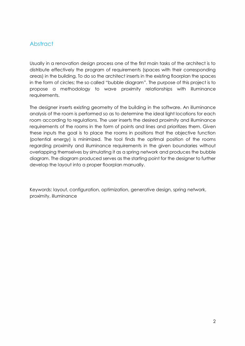
Abstract

Usually in a renovation design process one of the first main tasks of the architect is to

distribute effectively the program of requirements (spaces with their corresponding

areas) in the building. To do so the architect inserts in the existing floorplan the spaces

in the form of circles; the so called “bubble diagram”. The purpose of this project is to

propose a methodology to wave proximity relationships with illuminance

requirements.

The designer inserts existing geometry of the building in the software. An illuminance

analysis of the room is performed so as to determine the ideal light locations for each

room according to regulations. The user inserts the desired proximity and illuminance

requirements of the rooms in the form of points and lines and prioritizes them. Given

these inputs the goal is to place the rooms in positions that the objective function

(potential energy) is minimized. The tool finds the optimal position of the rooms

regarding proximity and illuminance requirements in the given boundaries without

overlapping themselves by simulating it as a spring network and produces the bubble

diagram. The diagram produced serves as the starting point for the designer to further

develop the layout into a proper floorplan manually.

Keywords: layout, configuration, optimization, generative design, spring network,

proximity, illuminance

3

Contents

Abstract ............................................................................................................................... 2

1 Introduction .................................................................................................................. 5

1.1 Background & necessity ...................................................................................... 6

1.2 Motivation ............................................................................................................. 6

1.3 Conventional methods ........................................................................................ 6

1.4 Knowledge gap .................................................................................................... 6

1.5 Research objective .............................................................................................. 7

1.6 Research question ................................................................................................ 7

1.7 Scope .................................................................................................................... 8

1.8 Problem statement ............................................................................................... 9

1.9 Advantages ........................................................................................................ 12

1.10 Challenges .......................................................................................................... 12

1.11 Assumptions ........................................................................................................ 12

1.12 Limitations ............................................................................................................ 13

1.13 Scientific and societal relevance ...................................................................... 13

1.14 Research methodology ..................................................................................... 14

1.15 Related tools ....................................................................................................... 16

1.16 Outline ................................................................................................................. 16

2 Background knowledge ........................................................................................... 17

2.1 Generative design .............................................................................................. 18

2.2 Gradient descent ............................................................................................... 18

2.3 Newton’s laws ..................................................................................................... 20

2.4 Hooke’s law ......................................................................................................... 21

2.5 Elastic energy ...................................................................................................... 22

2.6 Spring network .................................................................................................... 23

2.7 Force directed graph drawing .......................................................................... 26

2.8 Kangaroo ............................................................................................................ 29

2.9 Literature review ................................................................................................. 30

3 Proposed methodology ............................................................................................ 37

3.1 Case study .......................................................................................................... 38

3.2 Context ................................................................................................................ 39

4

3.3 Existing floorplan ................................................................................................. 41

3.4 Design assignment .............................................................................................. 45

3.5 Program of requirements ................................................................................... 46

3.6 System of modules .............................................................................................. 48

3.7 Bubble diagram .................................................................................................. 51

3.8 Proximity requirements ....................................................................................... 51

3.9 Illuminance requirements................................................................................... 54

3.10 Tool development .............................................................................................. 58

3.10.1 Inputs ............................................................................................................ 62

3.10.2 Daylight simulation ...................................................................................... 65

3.10.3 Optimal configuration ................................................................................. 67

3.10.4 Outputs ......................................................................................................... 70

3.10.5 Calculations ................................................................................................. 71

3.11 Layout development.......................................................................................... 72

3.12 Design proposal .................................................................................................. 77

4 Evaluation................................................................................................................... 81

4.1 Evaluation of the tool ......................................................................................... 82

4.2 Evaluation of the design development ............................................................ 85

5 Conclusions ................................................................................................................ 89

Reflection .......................................................................................................................... 92

List of figures ...................................................................................................................... 95

Bibliography ...................................................................................................................... 98

Appendices..................................................................................................................... 101

Appendix A: Grasshopper script ................................................................................ 101

Appendix B: Pseudocode in Python .......................................................................... 128

5

1 Introduction

6

1.1 Background & necessity

Residential design has always been one of the most favorite and popular design tasks

for architects. And this is, in my opinion, because of the great importance of having a

suitable home. Throughout the years residential design has been evolved in different

ways all over the world. And it is or should be still evolving in respect to current situation

and users’ needs. But there was not always feasible to build a house from scratch. The

idea of reusing an existing building is not new; on the contrary it has been introduced

in multiple cases since ancient times [1]. Nowadays reuse still remains an important

topic not only because of lack of free space, but also from an economical and

sustainable point of view [2]. More and more architects explore ways of renovating

the interior or even the exterior when repurposing a building [3]. While renovation of

the exterior results in more specific solutions regarding mainly structural methods’

applications, renovation of the interior belongs essentially to the architectural field.

The present graduation research attempts to explore a systematic way of repurposing

the interior of an existing building to a residence using computational tools.

1.2 Motivation

From an architectural point of view any renovation design is very interesting because

of the extra challenge of the existing form of the building. From a societal point of view

renovation projects entail also sustainability purposes. In European Union there are

many countries that are facing a considerable housing problem such as the

Netherlands [4]. In the Netherlands many expats are arriving every year, and there is

not enough housing stock to accommodate everyone [5]. On the contrary, there is a

significant amount of buildings that are currently not in use and were originally

designed for non-residential purposes [6]. The goal of this graduation thesis is to

contribute to the repurpose of this kind of buildings so as to restrict the magnitude of

the housing problem.

1.3 Conventional methods

From relative research and personal experience it has been noticed that most

renovation methods apply to very specific scenarios [7][8][9]. Each renovation project

has a unique design solution that cannot be easily applied to other buildings. This

happens probably because conventional approaches of renovation projects

produce a limited amount of different results, mostly due to time restrictions the

architect has to face. In this context computer science can be the keystone to base

a kind of automated approach.

1.4 Knowledge gap

A field that belongs to computer science and is explored in the recent years in

architecture and civil engineering is generative design[10]. An intuitive definition of

generative design is described as an iterative design process where generation of

7

form is based on algorithms [11][12]. Generative design applications in architecture

are still emerging and that makes it difficult to find sufficient comprehensive

academic literature [13]. Having that in mind any academic contribution to the topic

is useful especially for future researches. This research aspires to contribute to this

knowledge gap by proposing a systematic approach regarding layout design in

renovation projects. In this way the housing problem not only in the Netherlands but

also worldwide could be approached with the proposed general procedure.

1.5 Research objective

The broader objective of the present research is to contribute to the systematization

of the renovation design process. A promising field for systematic approach seems to

be generative design [14]. Given specific restrictions and guidelines it is possible to

generate layouts according to the designer’s wishes. The proposed approach is a

systematic approach in which it is investigated until what point it is possible to

automate a part of the design process (semi-automation for the moment) in primary

design stage according to the user’s wishes (manual input) in respect to rooms’

connectivity (proximity of rooms) and illuminance requirements using computational

methods. A more detailed description of the methodology proposed is presented in

the Proposed methodology chapter.

Subgoals

1. To develop a method for finding an optimal position of the rooms in the layout

in respect to their connectivity in primary stage of renovation design process.

2. To develop a method for finding an optimal position of the rooms in the layout

in respect to illuminance requirements in primary stage of renovation design

process.

3. To create a methodology that applies these two methods using

computational tools.

1.6 Research question

The main research question of the graduation project can be formulated as: “To what

extent is it possible to convert an existing layout into a residential one regarding

proximity relationships and illuminance requirements using computational tools during

primary design stages?”.

Subquestions:

1. What method can be used to find the optimal position of the rooms in respect

to their proximity relationships in primary stage of a renovation design process?

2. What method can be used to find the optimal position of the rooms with

respect to their illuminance requirements in primary stage of a renovation design

process?

3. How to combine daylight and proximity preferences in one layout design

configuration?

8

4. Are existing plugins for Grasshopper useful for the thesis’ purposes?

Design assignment

The main delivery assignment is the methodology for applying computational

methods to convert an existing layout into a residential one regarding proximity and

illuminance requirements during primary design stages. A basic case study will be used

to demonstrate the process in a simpler form. To evaluate the methodology two more

complex applications will be used to test the effectiveness of the tool. The tool is not

expected to be fully automated but to serve as a guide that gives more freedom to

the designer to customize the renovation design process according to his/her

preferences. The tool development is explained in detail in the present report and the

script of the tool will be added in the appendix so as to ensure transparency and

reproducibility of the process.

1.7 Scope

As it can be seen in the Venn diagram depicted in figure 1 the main focus areas of the

research are architecture (design criteria) and computational design (generative

design). Climate design and physics are essential for simulating real world situation that

are used in the tool, such as daylight and physics analysis.

Research scope includes:

layout

proximity

illuminance

optimization

algorithmic design

Research scope does not include:

facade

structure

ventilation / HVAC system

odor/ thermal / light comfort

furniture arrangement

real estate

fire safety

local climate conditions

thermal requirements

other daylight requirements

window to wall ratio

BIM

urban context

furniture arrangement Figure 1: Research scope

9

1.8 Problem statement

Renovation of buildings is a topic that concerns many architects all over the world.

Generative design seems a promising field to apply computational methods in the

primary design renovation process. To do so the design task has to be translated in

mathematical terms. The formulation of the part of the design process in a

mathematical way constitutes the part that will be attempted to be automated. The

approach constitutes basically the development of an algorithm whose parts are a

combination of manual and automated subtasks. In some cases the manual work is

legitimate as for example the inputs (building, program of requirements, desired

proximity between rooms) and in others it is a limitation due to computational power

or lack of advanced programming skills.

Usually in a renovation design process one of the first main tasks of the architect is to

distribute effectively the program of requirements (spaces with their corresponding

areas) in the building. To do so the architect inserts in the existing floorplan the spaces

in the form of circles; the so called “bubble diagram”. A bubble diagram is a simple

diagram of rooms shaped like circles whose purpose is to understand the relationship

between rooms. The purpose of the tool is to wave the room relationships with the lux

requirements. Apart from the question “what is the optimal room arrangement based

on my desired relationships?” the tool assists the architect answer also the question

“what is the optimal room arrangement based on the relationships and the

illuminance requirements?”.

For this reason, a graph is used to express mathematically the problem. The vertices

of the graph indicate the rooms’ positions, whereas the edges their connectivity. In

the following figure:

vertices as room centroids and edges as their proximity connections (in

red).

vertices as ideal illuminance position and edges as the connections

with the room centroids (in green)

vertices’ final position where both requirements are fulfilled as much as

possible (in blue).

10

Figure 2: graph representing the problem in a simple form where a, b, c the initial room positions, a’, b’,

c’ the ideal illuminance positions and af , bf , cf the final room positions

The edges of the graph are weighted with a factor (0/0.5/1) so as to prioritize their

importance, as it can be seen in the following tables:

Figure 3: adjacency matrix for proximity connections

Figure 4: adjacency matrix for illuminance connections

The graph is simulated as a spring network, where the weight of the edges is expressed

by stiffness.

The objective function is the minimization of elastic potential energy

𝑈 = 1

2𝑘 𝑥2

where 𝑘 stiffness is the constant

𝑥 position is the unknown/variable

constraints 𝑥 ≥ 0 and 𝑘 ≥ 0.

(The approach is presented more clearly in the following chapter.)

The major steps of the methodology are illustrated in the following figure. The designer

inserts existing geometry of the building in the software (step 1). An illuminance

analysis of the room is performed so as to determine the ideal light locations for each

room according to regulations (step 2). The designer inserts the desired proximity and

illuminance requirements of the rooms in the form of points and lines (step 3). Given

11

these inputs it is desired to find a position for the rooms such that the objective

functions is minimized. The tool finds the optimal position of the rooms regarding

proximity and illuminance requirements in the given boundaries without overlapping

themselves by simulating it as a spring system in the form of a bubble diagram (step

4). The configuration produced serves as the starting point for the designer to further

develop the layout into a proper floorplan manually (step 5).

Figure 5: Problem statement Step 1: empty existing building, Step 2: calculate illuminance values of test

points on grid Step 3: set room’ centroids and their proximity requirements as line segments, Step 4: final

configuration of rooms based on proximity and illuminance requirements set are shown as bubble diagram,

Step 5: final layout based on the bubble diagram

12

1.9 Advantages

Some of the advantages of formulating the design problem as a mathematical

problem are:

Innovation

Contribution into filling the knowledge gap that exists in the computational

literature.

Complexity

A large complex building can be divided into smaller parts. Iterations of

processes can be relatively easy to handle by computers once they are set in

the correct procedure.

Data structure

A lot of data can be stored in a mathematical way so that they can be

accessed more easily (matrices).

Time-saving

Once the workflow is set it will be much quicker to find the optimized layout for

different specifications.

Money-saving

As a result of time saving. [15]

1.10 Challenges

Challenges of formulating the design problem as a mathematical problem:

Advanced mathematics

A Building Technology student does not have the necessary background

knowledge to use advanced mathematics.

Data oversimplification

Data simplification should not be too abstract to be realistic.

Technicalities

The programming background level to tackle the topic fully computationally

does not correspond to that of a Building Technology MSc student.

Bugs

Debugging can be time-consuming and requires advanced programming

skills.

1.11 Assumptions

This tool is intended to be used by architects, interior designers and students during

the early design phases so as to have a quick intuition of how the arrangement of the

rooms affects the user’s movements (proximity) and visual comfort (illuminance). It is

assumed that the user already knows the basic commands of Rhinoceros and

Grasshopper software.

13

In order for the design assignment to be translated in a mathematical problem it is

inevitable to simplify reality. This refers to simulations run by software that simulate

approximately natural phenomena such as spring transformation, body collision,

daylight, etc. Since the design is a renovation assignment there are some elements

that are assumed to remain fixed and untouched. These elements are the building’s

core, rest bearing elements (structural walls, columns), HVAC system, etc. The whole

façade is assumed to be from standard materials and any improvement falls out of

the scope. Even windows are considered to have standard material properties that

are used in daylight simulation but any improvement falls also out of the scope.

1.12 Limitations

In case the bubble diagram produced by the tool is not satisfactory the process has

to be repeated from the beginning. Moreover, the tool considers a limited amount of

design criteria (proximity and illuminance only), but the design criteria an architect

takes into consideration are much more (e.g. privacy, safety, view, circulation,

supervision). Also the tool ignores the existence of obstacles in the interior of the

building (such as columns and walls). These have to be manually excluded from the

area of interest or the user has to take it into account during the manual design

development phase. Additionally, the tool is designed for 2D drawings only. The

illuminance values in reality would be much more different since the illuminance

analysis at first is made with open floor plan, which is usually not the case in the final

floorplan.

1.13 Scientific and societal relevance

As far as society concerns, renovation was and still is an import design assignment,

especially in countries where its available to build area is limited. Converting existing

buildings into residences is a way to tackle the housing problem many people (locals

and expats) from all over the world face. In a professional point of view, finding a way

to systemize the renovation design process could have a great impact on the way

architects would approach a renovation project since the very beginning. As soon as

they have an initial design idea by following the suggested methodology it would be

possible to insert the necessary data and produce the schematic residential layout

based on the two –most important according to the author- design criteria: proximity

and daylight. One of the main advantages of computational applications is that they

can handle a respectable amount of data simultaneously. This means that many

levels of complexity can be added to the tool and in that way help the architect find

the optimum layout. This could speed up the design process and also produce non-

conventional but still functional layouts.

The current graduation project is directly related to MSc Architecture, Urbanism and

Building Sciences and the Building Technology track. Firstly, the computational

methods proposed are intended to be applied in existing buildings, in real life

scenarios, which is what architecture and building sciences is about. The case study

14

selected empower the practicality and the usefulness of the tool and is itself a

property of TU Delft (Faculty of electrical engineering, mathematics and computer

science) . The intention to contribute in the systemization of the renovation design

process is an architectural intention interwoven with sustainability, that is one of the

main aspects of Building Technology track. Building Technology is also the field where

architects are more oriented towards engineering. Mathematics and physics are

some of the fundamental subjects of an engineer. Engineering is also about improving

existing methods as well as inventing new ones. In this dissertation the innovation lies

in developing a methodology on how to systemize a renovation design project using

principles of computer science, mathematics and physics.

1.14 Research methodology

The first step in the graduation research is to formulate the research framework. In

order to define the research objective a research of the relative background and the

conventional methods of renovation design processes was conducted to spot the

knowledge gap. After having set the research objective the research question and

subquestions has to be defined in a more clear way.

The second step is to obtain the necessary theoretical background. This includes

reading relative literature regarding generative design in layout applications,

exploring existing commonly used parametric tools and finding a representative case

study to apply the proposed methodology.

During the third step the specifications and assumptions are set so as to start the tool

development. In the beginning the main skeleton of the tool is defined by relative

research and it is fully developed when applied in the case study. By following the

proposed methodology it is possible to produce and evaluate the outputs. If the result

is not satisfactory the process has to be repeated but this time the chosen parameter

should be shifted slightly to observe its impact. By repeating and improving the tool

starts to take its final form.

In more detail, the tool is developed in five stages: the first stage starts with all

necessary input set by the user, then an illuminance analysis is performed in order to

obtain the lux values, afterwards the optimal configuration is found by performing

dynamic relaxation. The configuration is later evaluated based on proximity and

illuminance requirements set at the beginning. The output of the tool is a schematic

layout (bubble diagram) indicating the ideal position of the rooms as well as their

corresponding lux values.

The evaluation step is a test to check how the tool performs in larger and more

complex cases. The last step includes the discussion upon the results, the conclusions

drawn from the discussions and recommendations for improvement of the tool and

further research.

15

Figure 6: Research methodology workflow

16

1.15 Related tools

The following software applications are related to the scope of this research in that

they provide various methods of modeling and processing data.

The main software to be used:

Rhinoceros by Robert McNeel & Associates (CAD) [16] and

Grasshopper by David Rutten, Robert McNeel & Associates (visual

programming) [17]

The plug-ins for Grasshopper required are:

KangarooPhysics & Kangaroo2 by Daniel Piker (physics simulation) [18]

Honeybee & Ladybug by Mostapha Sadeghipour Roudsari (daylight

simulation) [19]

GH Python by Guilio Piacentino (IronPython included in GH) [20]

GH CPython by Mahmoud Abdel Rahman (python scripting) [21].

1.16 Outline

The report begins with the introduction where a brief overview of the graduation

research is presented. The next chapter Background knowledge aims at clarifying

some of the methods and techniques used while developing the tool. The tool

development is described in detail in chapter 3 Proposed methodology. As an

example for demonstration purposes a representative case study (studio) is used,

namely Case study I (EEMC). For evaluation purposes two more applications in the

same building will be examined (shared apartment and common facilities). The results

of the evaluation of the proposed methodology are presented in chapter 4

Evaluation. Afterwards, the main results of the research are discussed and the basic

conclusions are drawn. The last chapter of the report contains the personal reflection

of the author upon the graduation thesis based on the requirements set by the faculty.

In short, the outline of the report look like this:

Chapter 1: Introduction

Chapter 2: Background knowledge

Chapter 3: Proposed methodology

Chapter 4: Evaluation

Chapter 5: Conclusions

Reflection

17

2 Background

knowledge

18

2.1 Generative design

An intuitive definition of generative design can be described as “an iterative design

process where generation of form is based on algorithms” [11][12]. The generative

design process is defined by applying constraints, parameters and goals to a project

and then exploring all possible design options through a series of iterations. A

generative design software (such as Grasshopper) then applies computational

algorithms, which generate the design according to the parameters set. Afterwards

designers can select the outcome that best meets their needs [22]. The following

figure shows the workflow of designing a product by using generative design process

[23].

Figure 7: generative design flowchart by H. Bohnacker [23]

2.2 Gradient descent

“Gradient-based methods are iterative methods that extensively use the gradient

information of the objective function during iterations.” For the minimization of a

function 𝑓(𝑥), the method can be described as:

19

where α is the step size that can take different values,

g(∇f,x(n)) is a function of the gradient ∇f and the current location x(n).[24]

By using an algorithmic gradient based approach to automate a generative design

process, the design outcome always goes towards the optimum solution.

“Gradient descent is the most common optimization algorithm in machine learning

and deep learning. (Optimization refers to the task of minimizing/maximizing an

objective function f(x) parameterized by x). In machine/deep learning terminology, it

is the task of minimizing the cost/loss function J(w) parameterized by the model’s

parameters w ∈ R^d.) Gradient descent is a first-order optimization algorithm. This

means it only takes into account the first derivative when performing the updates on

the parameters. The gradient gives the direction of the steepest ascent. On each

iteration, the parameters are updated in the opposite direction of the gradient of the

objective function J(w). The size of the step we take on each iteration to reach the

local minimum is determined by the learning rate α. Therefore, it is followed the

direction of the slope downhill until a local minimum is reached.”[25]

A pseudocode for a gradient descent algorithm look like this:

Let’s say we want function J(𝑥1, 𝑥2) to be minimized:

1. Start with some values for 𝑥1, 𝑥2 (eg 𝑥1=0, 𝑥2=0)

2. Keep changing 𝑥1, 𝑥2 to reduce J(𝑥1, 𝑥2)

3. Repeat until convergence:

𝑥’𝑗 = 𝑥’𝑗 - a ∂/∂xj J(𝑥1, 𝑥2)

where:

a the learning rate

∂/∂xj J(𝑥1, 𝑥2) the derivative

4. Until 𝑥𝑗 = 𝑥𝑗

Figure 7 shows the relationship of the cost and weight function regarding the

derivative of function J, whereas the next one shows the result which is a local

minimum [26].

20

Figure 8: the graph of gradient descent algorithm in respect to cost and weight [26]

Figure 9: the three possible results of gradient descent: local minimum, global minimum and plateau

[26]

So, in this project it is aimed to find a local minimum and the learning rate used (a) is

small (0.1).

2.3 Newton’s laws

The following equations of Newton are used in the proposed algorithm, so this

section serves as a reminder.

First law: Inertia

∑ 𝐹 = 0

21

Second law: Acceleration

𝐹 = 𝑚 𝑎

Third law: Action-Reaction

𝐹𝐴 = −𝐹𝐵

Fourth law: Superposition

𝐹(𝑥1+𝑥2) = 𝐹𝑥1+ 𝐹𝑥2

F: force

m: mass

k: spring constant

a: acceleration

x: displacement

[27]

2.4 Hooke’s law

The algorithm proposed uses also Hooke’s law, which states that “ for relatively small

deformations of an object, the displacement or size of the deformation is directly

proportional to the deforming force. Under these conditions the object returns to its

original shape and size upon removal of the force.” [28]

𝐹 = 𝑘 𝑥

where 𝐹 : force 𝑘: stiffness

𝑥: elongation

22

Figure 10: Schematic explanation of Hooke's law[28]

2.5 Elastic energy

The objective of the optimization is to minimize the elastic potential energy. It is

reminded here that “elastic energy is energy stored as a result of applying a force to

deform an elastic object. The energy is stored until the force is removed and the

object springs back to its original shape, doing work in the process.” [29]

𝑈 =1

2𝑘 𝑑2

𝑈 = ∫ 𝑘 𝑥 𝑑𝑥 =1

2𝑘 (𝐿 − 𝐿0)2

𝐿−𝐿0

0

where 𝑈: elastic potential energy 𝐿: final length

𝐿0: initial length 𝛥𝑥, 𝑑𝑥, 𝑥: elongation

𝑘: stiffness

In the following diagram it can be noted that the area of the triangle formed by the

blue line and x axis is the actually the work. [29]

23

Figure 11: Force towards displacement diagram [29]

2.6 Spring network

A graph with vertices and edges can be simulated as a spring network, a physical

system drawn where the edges represent springs of given stiffness and length. In the

case of this research the vertices can represent the centroids of the rooms (as points)

and the springs the connections between them (as line segments). Assuming linear

springs, where no energy is lost and no rotation, twisting or deformation is involved,

the spring system can be considered as a system of linear equations or, equivalently,

as an energy minimization problem (minimization of elastic potential energy).

As input from the user inserts points that represents the position

of the centroids of each room, e.g. point A.

These points are placed in initial random positions inside

the building’s boundaries.

All points (vertices) are interconnected with straight line

segments (edges) , from which it is derived their Euclidean

distance 𝑥. The set of vertices and edges forms a graph.

24

Almost every pair of vertices is connected with an edge

(fictitious mechanical spring) representing their type of

connection. There are three types of connections expressing

the hierarchy (strong, medium and weak) and thus three types

of springs with different values of the spring constant 𝑘1, 𝑘2 , 𝑘3.

All springs have the same rest length x0 = 0 m. All distances between

centroids should be more than 0, so x > x0 . This means that once the

springs are attached to the centroids all of them are under tension x1

> x0.

25

At point Γ external forces occur. These forces can

be calculated by applying Hooke’s law:

𝐹1 = 𝑘1 (𝑥𝛤𝛣 − 𝑥0)

𝐹2 = 𝑘2 (𝑥𝛤𝛦 − 𝑥0)

𝐹3 = 𝑘3 (𝑥𝛤𝛢 − 𝑥0)

The resultant force at point Γ is vector sum of all forces

acting upon it:

∑ 𝐹𝛤 = �⃗�1 + �⃗�2 + �⃗�3

The resultant force can be calculated by using the

polygon rule.

The same process is repeated for all points.

The elastic potential energy for one spring is:

𝑈𝛦𝛤 =1

2𝑘2(𝑥 − 𝑥0)2

If n1 the number of springs that have spring constant k1 and x1

their corresponding deformation, then the total elastic potential

energy of the system Utot can be calculated by:

Utot =1

2k1(x1 − x0)2 +

1

2k2(x2 − x0)2 +

1

2k3(x3 − x0)2

26

By setting the springs free they tend to reach their original rest

length, so they tend to approach each other because the rest

length x0 was set to be 0. The system will try to reach to an

equilibrium where Utot is minimum.

The objective is to find new positions of the points (A’, B’, Γ’, Δ’, Ε’) that fulfill the

proximity requirements. The objective in terms of physics could be expressed as to

minimize the potential energy of the springs. A way to do so is by using gradient

descent methods such as force directed graph drawing developed by P. Nourian and

S. Azadi.

2.7 Force directed graph drawing

P. Nourian and S. Azadi. have proposed “a ‘force-directed graph-drawing algorithm

to draw a bubble diagram based on nodes, links, and the intended area for the

nodes. This way, the designer does not need to manage to draw a neat diagram, as

the system does it for them.” [30] The pseudocode is presented below:

Input: the graph Γ (V, E), E = (Vi, Vj) if Vi is linked to Vj

Step 1: Compute resulting forces:

Resulting_forces = ∑Attraction_forces(v) + ∑Repulsion_forces(v)

u = u moved by Resulting_forces

Step 2: Recompute Continuance_condition:

∀(i,j)∈E, xij (Ri+Rj) +- ErrorTollerance

Step 3: Iteration_count = iteration_count + 1

Until Continuance_condition=False or Iteration_count > Maximum_iterations

Output: a kissing-disk drawing of graph Γ

where

Attraction_forces = AFij = ka Δxij

ka = attraction strength factor,

Δxij = Distance Vi to Vj - RestLength(i,j),

RestLength(i,j) = Ri+Rj

Repulsion_forces = RFij = kr / xij ∀(i,j) if xij < RestLength(i,j)

kr = repulsion strength factor,

xij = Distance Vi to Vj

RestLength(i,j) = Ri+Rj

[30]

Based on the above algorithm the approach proposed in this project is also a gradient

descent based approach. It is a numerical method that attempts to minimize the

27

potential energy of a spring network. The method 𝑥(𝑛+1) = 𝑥𝑛 + 𝑎 𝑔(∇𝑓, 𝑥𝑛) of gradient

descent in this case is:

𝑣′𝑖 = 𝑣𝑖 + 0.1 𝛴𝐹𝑖𝑗

where 𝛴𝐹𝑖𝑗 = 𝐹𝑖𝑗 + 𝑅𝑖𝑗

In more detail, given a vertex 𝑣𝑖 and 𝑣𝑗 its neighbor vertex both

representing the initial positions of two rooms.

The areas of the rooms are represented with a circle with

corresponding radii 𝑟𝑖, 𝑟𝑗 and centers the vertices 𝑣𝑖, 𝑣𝑗

respectively.

The line segment connecting the two vertices is called edge 𝑒𝑖𝑗.

The edge has a specific stiffness value 𝑘𝑖𝑗.

The edge has also a set length 𝑑𝑖𝑗 , the distance between the

two vertices 𝑣𝑖, 𝑣𝑗 that is calculated by: 𝑑𝑖𝑗 = 𝑣𝑖 − 𝑣𝑗

The proximity requirements of the rooms are expressed by an

attractive force that tries to place the rooms closer with each

other. The strength of the force is defined by the edge’s stiffness

and distance: 𝐹𝑖𝑗 = 𝑘𝑖𝑗 ∗ 𝑑𝑖𝑗

In case the distance between the vertices is smaller than the sum

of their radii (𝑖𝑓 𝑑𝑖𝑗 < 𝑟𝑖 + 𝑟𝑗) then a repulsive force 𝑅𝑖𝑗 is added

to avoid collision. This force acts in the opposite direction of the

attractive one and is defined by another stiffness value 𝑘𝑟 and

the distance: 𝑅𝑖𝑗 = −1 ∗ 𝑘𝑟 ∗ 𝑑𝑖𝑗

The resultant force 𝛴𝐹𝑖𝑗 is the algebraic sum of the forces acting

on vertex 𝑣𝑖 : ∑ 𝐹𝑖𝑗 = 𝐹𝑖𝑗 + 𝑅𝑖𝑗

After we have the direction of the resultant force ∑ 𝐹𝑖𝑗, the vertex

𝑣𝑖 is moved slightly towards this direction to approach its neighbor

vertex 𝑣𝑗 , so: 𝑣′𝑖 = 𝑣𝑖 + 0.1 ∗ ∑ 𝐹𝑖𝑗

The process is repeated for all vertices until the system is

converged, where the distance between the vertices is as close

as possible to the sum of their radii: |𝑑𝑖𝑗|

𝑟𝑖+ 𝑟𝑗 − 1 < 0.0001 or the

maximum number of allowed iterations is reached.

28

This method fulfills the proximity requirements of the rooms. In the same logic the

illuminance requirements are expressed as proximity requirements (strong

connections) between the room and its ideal position in the building regarding

illuminance.

As seen in problem statement paragraph, the vertices of the graph indicate the

rooms’ positions, whereas the edges their connectivity. In the following figure:

vertices as room centroids and edges as their proximity connections (in

red).

vertices as ideal illuminance position and edges as the connections

with the room centroids (in green)

vertices’ final position where both requirements are fulfilled as much as

possible (in blue).

Figure 12: graph representing the problem in a simple form where a, b, c the initial room positions, a’, b’,

c’ the ideal illuminance positions and af , bf , cf the final room positions

In order to define the illuminance requirements an illuminance analysis is performed

and a grid of test points (fixed locations) is created all over the buildings’ surface

(floor). The test points with the required illuminance value that is the closest to the initial

room’s position is selected (a’, b’, c’) and an edge that connects them with the

corresponding room is created (green line segments). The green edges that express

the illuminance requirements are considered in the above mentioned algorithm in the

same way as proximity connections.

Taking into consideration the above mentioned algorithm the resultant force is:

for proximity:

∑ 𝐹𝑝 = 𝐹𝑝 + 𝑅𝑝

𝐹𝑝 = 𝑘𝑝 ∗ 𝑑𝑝

𝑅𝑝 = −1 ∗ 𝑘𝑟 ∗ 𝑑𝑝

for illuminance:

∑ 𝐹𝑖 = 𝐹𝑖 + 𝑅𝑖

29

𝐹𝑖 = 𝑘𝑖 ∗ 𝑑𝑖

𝑅𝑖 = −1 ∗ 𝑘𝑟 ∗ 𝑑𝑖

in total:

∑ 𝐹𝑡 = 𝐹𝑝 + 𝑅𝑝 + 𝐹𝑖 + 𝑅𝑖

After the direction of the resultant force ∑ 𝐹𝑡 is known, each vertex is slightly moved

towards this direction : 𝑣′𝑖 = 𝑣𝑖 + 0.1 ∗ ∑ 𝐹𝑡

The objective function is then: 𝑈 = 1

2𝑘𝑝 𝑑𝑝

2+

1

2𝑘𝑖 𝑑𝑖

2

2.8 Kangaroo

The iterative process of the above algorithm is performed by Kangaroo engine, but

ideally it should be developed in Python within Grasshopper. An attempt of

developing it in Python can be found in appendix B; it was not completed due to time

restrictions of the thesis.

Grasshopper is “a visual programming language and environment that runs within the

Rhinoceros 3D CAD application” (by D. Rutten, Robert McNeel). [31] [17] Kangaroo is

“a Live Physics engine for interactive simulation, form-finding, optimization and

constraint solving developed by D. Piker. It is an add-on for Grasshopper/Rhino which

embeds physical behaviour directly in the 3D modelling environment and allows user

to interact with it 'live' as the simulation is running.” [32]

Kangaroo is not open-source to be able to study how it works, but as the developer

reveals “Kangaroo works by finding the total force vector F for each particle by:

adding up all the different forces acting on it,

using Newton's 2nd law to get the acceleration,

and numerically integrating the resulting differential equation of motion over

time to find new positions for all the particles.” [33]

Moreover, “a point in Kangaroo reaches equilibrium when the weighted average of

the move vectors from all goals acting on it is zero. The solver can also be seen as a

minimization of the (weighted) sum of the squares of the distances from the rest

positions for each goal acting on each point.”[34]

30

2.9 Literature review

The topic of this thesis is relatively new so the most relevant existing literature are

academic projects by individuals. The first three projects use parametric tools as the

design environment, while the last two make use of graph theory in their approach.

Graph theory is not the approach for this thesis but was used as an inspiration only

(graph, adjacency matrix). The project closes to the approach proposed is

“Architectural space planning using parametric modeling” by M. Elsayed where he

also simulates the problem as a physical system. During the research some other

projects developed by students were found but were not officially published and or

well documented and therefore were not included in the review. The overall

impression is that there are many gaps in relative literature and every attempt is

beneficial.

Rapid Data Collection using Automated Model Generation and Performance

Evaluation

The first part of the project is a proposal of a workflow for speeding up the collection

of data from apartment floorplans. In the second part a tool for automated model

generation and evaluation is suggested. The purpose of the tool is to find the relations

between various design variables and selected performance criteria. Some of the

design variables are: number of rooms, their relevant position, dimensions, walls,

windows and some of the design criteria are: daylight (daylight factor), energy

consumption (window layout, orientation), common quantities (total area, effective

area, number of rooms, neighboring and interior walls). [35]

The software selected is Rhinoceros and Grasshopper and two main plugins used are

Decoding Spaces Toolbox (for layout generation) and Diva (for energy simulation).

[35]

31

Figure 13: Different analysis diagrams for one apartment floor plan [34]

32

Computational Floorplan Synthesis

In this book the first chapters are dedicated to ALES projects, a general layout design

system. Based on ALES the research project KREMLAS explored various methods for

automatic floorplan generation. The methods explored to produce layouts were

based on a) the principle of tight packing of geometric elements (dense packing), b)

K-dimensional trees c) subdivision algorithms, d) voronoi diagram.

The two main requirements were a) the sizes of the desired rooms and b) their

topological neighborhood relationships (which room should be next to which).

The proposed system generates automatically a geometrical solution and it can

adapt the geometry to new requirements. Apart from that an additional study

evolved the generation of a floorplan by dense packing with visibility evaluation. [36]

Figure 14: links of rooms with dense packing and respective door placement [35]

Figure 15: alterations of rooms' arrangement together with possible visibility offered by the doors [35]

33

Evolutionary parametric analysis for optimizing spatial adjacencies

This paper utilizes Grasshopper as a planning tool to graphically represent a 3-

dimensional analysis of adjacency requirements in program and spaces. The purpose

of this project is to investigate whether there are new ways to use evolutionary

algorithms so as to optimize floorplan layouts. A tool developed in Grasshopper is

proposed and it generates diagrammatic layouts based on given adjacency

requirements. The inputs are simple geometry representing the building’s rooms

(perimeter, height, area). The proximity is determined by the distance between each

origin point of the rooms. The optimization tool Galapagos tries to minimize this

distance and produces the most suitable arrangement of the all volumes (rooms) set

within the larger volume (building). [37]

Figure 16: input: geometry as circles and height, output: pixelated, extruded and arranged volumes [36]

Architectural space planning using parametric modeling

This paper proposes an automatic multi-stories space planning tool. The investigated

method uses two kids of physics simulation: a) mechanical springs and b) boxes

collision so as to rearrange the position of the rooms (attraction to the vertical core).

The main tools utilized are Grasshopper, Microsoft Excel (for the inputs) and Kangaroo

(for physics simulations). Some of the inputs are number of spaces, spaces proximity,

floor height. The output of the first simulation is the position of the spaces after the

spring forces have been applied and of the second simulation is the compact

rearrangement. [38]

34

Figure 17: The simulation process: a) The initial position of spaces showing volumes and springs action

directions. b) Spaces behavior under spring forces. c) First simulation result. d) Second simulation result.

[37]

Production layout optimization for small and medium scale food industry

This study aims to create a production layout for a food company using facility

planning techniques. The first phase is the generation of layouts using two different

types of construction techniques Systematic Layout Planning (an 11-step procedure)

and Graph Based Theory (adjacency and design phase). The second phase is the

calculation of the Efficiency Rate (sum of department adjacency score/sum of

relationship score). The layout with the highest ER was selected and then improved

using Pairwise Exchange Method.

The software used was MATLAB and the input was the order of the different

departments in a spiral way, the number and size of the machines as well as the

required area around them. The output was the improved order of the departments

again in spiral way. [39]

35

Figure 18: Relationship chart [38]

Figure 19: Space relationship [38]

36

Parallel planning: An experimental study in spectral graph matching

One project of this research is to design a prototype of a spatial configuration defined

by a graph so that it can be applied to an existing configuration using spectral graph

theory (for matching the two graphs).

Based on an existing spatial structure an adjacency graph is computed first. Next a

bubble diagram shows the desired spatial configuration. Inexact Graph Matching is

used to match the desired configuration with the existing one. The matching is

improved by applying a hill climber algorithm resulting in the desired layout. The results

show that in two from 30 cases a correct matching was found. (The tools used, inputs

and outputs were not mentioned in this paper.) [40]

Figure 20: An existing floor plan with a spatial subdivision and pre-matches; Bubble diagram of functions

(with relative sizes); The initial spectral matching (normalized-Laplacian matrix and UPGMC,

Renormalized); Improved matching through a hill climber. [39]

37

3 Proposed

methodology

38

3.1 Case study

As a case study that would be representative and useful for the application of the

proposed methodology was selected the Faculty of Electrical Engineering,

Mathematics and Computer Science (EEMC). It is a large building complex situated

at the center of the T.U. Delft campus, in Mekelweg 4. The building was conceived

from the start as the place that would host the department of Electrotechnical

Engineering. Designed by G. Drexhage in 1959, it contains a 92-meter tall building that

is a landmark for the entire city of Delft, rising higher than the church towers at the

center of the city. Its construction started in 1962 and was finished only in 1972,

spanning through an entire decade. EWI stands for Electro (electrical), Wiskunde

(mathematics) and Informatica (computer science), the three studies that are

located in the building. EEMC is considered to be the most recognizable faculty of TU

Delft University, a tall monument with 23 floors.

Figure 21: Photo of EEMC in Delft (from ground level) [52]

39

Figure 22: Photo of EEMC in Delft (aerial view) [41]

3.2 Context

The EWI building is currently considered a listed monument in the Delft landscape. But

EWI is also well known for having very strong winds around it, generated by the shape

of the building. [42] These functional problems arouse is a lot of discussion around

whether it should be demolished or not. This year (2020) it is said that the facade has

reached the end of its lifespan and therefore should be replaced. One of the

proposals considered is to change also the functions of the complex. In this context,

it could be transformed from the home of the electrical engineering faculty to a

student center and accommodation [43]. Taking the above into account EEMC

constitutes an ideal case study as it is a) a listed building (its cell should not be

changed), b) it is already discussed to be transformed into student housing, c)it is

located in Delft, that faces a shortage of residences in comparison to the high

demand due to the University. A tool that converts an existing layout into a residential

one (Cochleas) can be considered ideal to EEMC case.

40

Climate analysis

As it can be seen in the following figures, the central entrance of EEMC is at Northeast,

the sun is at the southern side during summer months and the dominant wind blows

towards Southwest.

[44]

Figure 24: Orientation of EEMC [46]

Figure 23: Screenshot from google maps indicating the

location of EEMC [45]

41

Figure 25: Direct sunlight analysis of EEMC for July [46]

Figure 26: Dominant wind analysis for EEMC [46]

3.3 Existing floorplan

The ground floor of EEMC accommodates a reception, a meeting area, halls, lecture

rooms and two large amphitheaters. The floorplan of the ground floor can be seen in

the figure below: [45]

42

Figure 27: Ground floor layout of EEMC [45]

43

The tower

The main area selected to apply the proposed methodology is located at the tower,

because the tower is the main concern of the TU Delft community and one of the

most problematic elements. Moreover, since there was no access to the floorplans of

the rest floors it is assumed that they are identical. The tool was applied also on the

ground floor, because it includes and additional part apart from the tower.

Interior

The EEMC complex accommodates three faculties: electrical engineering,

mathematics and computer science. It includes eleven lecture rooms, workshops and

laboratories. Most lecture room and halls are located at the ground floor whereas labs

and offices are located at the upper floors. As for its basic structural system, it consists

of concrete walls and steel columns. [44]

Figure 29: perspective view of the main corridor at the tower (existing situation) [44]

Figure 28: Layout of a typical floor of the tower of EEMC [45]

44

Figure 30: schematic representation of the structural system a typical tower’s floor [46]

The following pictures give an idea of the existing situation in the interior of EEMC. [46]

Figure 31: photo of the interior of the main corridor at the 21st floor [48]

Figure 32: photo of hall L located at the ground floor [47]

45

3.4 Design assignment

The hypothetical client of the design renovation assignment is supposed to be TU Delft

because it is its property. For this thesis’ purposes it is supposed that TU Delft wants to

repurpose the building and convert it into student housing. The relevant authorities

decide to create an architectural competition for this. An architecture office/ student

wants to participate in the competition and decides to use Cochleas during the

primary stages of the design so as to speed up the design process. For the purposes

of this graduation topic the author acts as the architect participating in the

competition and as the developer of Cochleas. The main requirement of the

competition is to accommodate 500 students and cover 3000 m2 of common facilities.

The EEMC building will be divided vertically regarding three floor types A,B and C.

Floortype A: studios

Floortype B: shared apartments

Floortype C: common facilities

Floortype D: ground floor

Figure 33: Table with units and residents numbers

46

Figure 34: Vertical arrangements of uses

Floor area (in grey and pink): 1035 m2

Two main parts to be rearranged (in pink): 746 m2

Figure 35: Area of interest (in pink) in a typical floor of the tower

3.5 Program of requirements

The area of application is expected to be converted into a studio apartment for one

person. The total square footage was set to be 26 m2, which is a relative typical size

for studio apartments in the Netherlands. A usual program of requirements includes a

patio, a kitchen, a living room, a bedroom, a restroom and, occasionally, a desk, a

storage room and a closet. The following table shows the rooms set by the user

47

together with their corresponding desired areas. The procedure of how the area

values were calculated is shown in the next paragraph.

Figure 36: Program of requirements for unit A (studios)

Figure 38: Program of

requirements for unit B

(shared apartments)

Figure 37: Program of

requirements for unit C

(common facilities)

Figure 39:Program of

requirements for unit D

(common facilities at

ground floor)

48

3.6 System of modules

In order to standardize interior configuration it was decided to use a modular system.

The module was set to be a square of 0.50 x 0.50m. The square size makes it convenient

to be multiplied in x and y direction and also it is in the allowable limits for an

illuminance analysis according to NEN (see paragraph “Illuminance requirements”).

The half a meter size is considered to be handy because the combination of two tiles

(resulting in 1m width) can form a corridor, a door, or a window. The combination of

four modules forms one square meter that is the typical unit of measuring area. The

module is used to find the minimum area needed for each room by arranging the

required furniture in relation to these modules. For defining an efficient required area

of a room it was useful to first set the required area for each room and then add extra

space for movement (such as corridors).

Module size:

For studios, different arrangements of furniture were made in Rhinoceros software

always based on the modules. Below is presented a sample of the experimentations.

The same method was applied for all units.

49

The minimum square footage of rooms as wells as the correspondent number of

modules 0.5x0.5m was calculated. Below it is presented an example for one studio of

26 m2 (type A).

Patio 1,50 m2 6 modules

Kitchen 3,00 m2 12 modules

Living room 6,25 m2 25 modules

Bedroom 5,00 m2 20 modules

Restroom 4,75 m2 19 modules

Desk 2,25 m2 9 modules

Storage 2,50 m2 10 modules

Closet 1,00 m2 4 modules

Total 26,25 m2 105 modules

Figure 40: configuration exploration based on the modules and minimum furniture required per room for

type A

50

An example of the experimentations regarding the furniture arrangement for

housing and common facilities can be seen in the following pictures:

Configuration of modules for residents

Configuration of modules for common facilities

51

3.7 Bubble diagram

The main goal of Cochleas is to help the user design a rough bubble diagram. Each

room can be represented as a circle (bubble). Each centroid is used as the center of

the circle. The lines connecting the centroids represent the connections between the

rooms. For the purposes of the graduation project the design criteria upon which the

bubble diagram is drawn is proximity and illuminance. Proximity was selected as it

reflects connections, movements of people and much more. Nevertheless, this is the

most common reason to use a bubble diagram. Illuminance was selected as a form

of indicating the daylight in the interior that is also very essential criterion for

architectural layouts. Of course an architect takes into consideration many more

criteria simultaneously such as view, routes, privacy, constructability, etc but it is not

possible of course to substitute the role of the architect with just one tool. Under this

spectrum the two most important criteria were decided to be proximity and

illuminance.

Levels of abstraction:

schematic layout => bubble diagram => graph

In this thesis the opposite process is attempted, meaning from an abstract topology

such as the graph, to find a bubble diagram and then to form a layout.

3.8 Proximity requirements

In order to construct the bubble diagram the REL-chart has to be decided first. The

REL-chart is actually a chart that indicated the relationship (proximity) of one room to

another. A new REL-chart has to be made for each unit (studio, shared apartment,

common facilities). Below are presented the REL-charts for each unit (A, B, C, D).

52

REL-chart

Figure 41: REL-chart for studios (type A)

Figure 42: REL-chart for shared apartments (type B)

53

Figure 43: REL-chart for common facilities (type C)

Figure 44: REL-chart for common facilities at ground floor (type D)

54

3.9 Illuminance requirements

Daylight can contribute significantly to the lighting needs of any type of building. The

evaluation of daylight provision should make account of the availability of daylight at

the site in addition to accounting for the properties of the space (e.g. external

obstruction, glazing transmittance, thickness of walls, internal partition and surface

reflectance, furniture, etc).

Criteria for daylight provision

A space is considered to provide adequate daylight if a target illuminance level is

achieved across a fraction of the reference plane within a space for at least half of

the daylight hours. The reference plane of the space is located 0,85 m above the floor.

Values for target illuminances, minimum target illuminances and fractions of reference

plane are given in Table A.1.

Figure 45: Recommendations of daylight provision [50]

Daylight Provision Calculation Methods

The following methods to assess daylight provision to the interior, using validated

software, are possible:

Method 1: Calculation method using daylight factors on the reference plane.

Method 2: Calculation method of illuminance levels on the reference plane

using climatic data for the given site and an adequate time step.

Calculation method using illuminance level (method 2)

Method 2 was selected as the calculation method to be performed in this project. This

method requires the use of a detailed daylight calculation method where hourly

internal daylight illuminance values for a typical year are computed using hourly sky

and sun conditions derived from climate data appropriate to the site. This calculation

method determines daylight provision directly from simulated illuminance values on

the reference plane.

55

Calculation grids

To determine target values of illuminances and daylight factors, it is necessary to

perform calculations over the entire reference plane, located 0,85 m above the floor

of the area to which they apply. The points at which calculations should be carried

out are defined in Formula (B.1). Grid cells approximating to a square are preferred,

the ratio of length to width of a grid cell shall be kept between 0,5 and 2. The

maximum grid size shall be:

[48]

Other guidelines regarding minimum recommended lighting levels for residential

spaces are presented below [49]:

Figure 46: Minimum recommended lighting levels for residential spaces [49]

56

After taking into consideration the above mentioned guidelines it was decided to

categorize the illuminance requirements into three main categories. The illuminance

requirements for the three units were formed as followed:

Illuminance categories:

Figure 47: illuminance categories with their respective minimum and target lux values

Below are presented the categorization of rooms for each type:

Figure 48: illuminance requirements for studios

Figure 49: illuminance requirements for shared apartments

57

Figure 50: illuminance requirements for common facilities

Figure 51: illuminance requirements for common facilities at ground floor

Daylight simulation

For daylight simulation the plugins Honeybee and Ladybug (both developed by M.

Roudsari ) are recommended to be used because they communicate smoothly

Grasshopper, are producing reliable results and are popular among architects. In

particular, Honeybee and Ladybug are Python librariesy to create, run and visualize

the results of daylight (RADIANCE) and weather files (EnergyPlus) respectively [50].

58

3.10 Tool development

Overview

The designer inserts existing geometry of the building and desired proximity and

illuminance requirements of the rooms. The tool finds the optimal position of the rooms

regarding proximity and illuminance requirements in the given boundaries. The

configuration produced serves as the starting point for the designer to further develop

the layout into a proper floorplan. In the next pages each milestone is presented in

more detail. In short the tool development stages are:

1. Inputs

2. Daylight simulation

3. Optimal configuration

4. Overlap

5. Outputs

The tool comprises of many components that made urgent to implement organisation

rules (chapters, groups, colour coding). There is colour coding for the input, data,

processes and output and extensive use of groups and notes throughout the

Grasshopper script so as to make it more clear to the user. All screenshots from the

final Grasshopper script are attached in the appendix. In the report only some

examples are presented whenever it is useful to visualize a process. In order to present

the tool as clear as possible the smallest application (unit A) is presented in detail in

the following paragraphs. For the rest units only the initial and final stages are

presented .

A flowchart of the tool is presented below:

Figure 52: colour coding rule

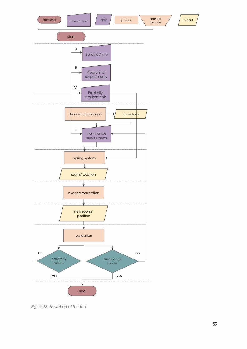
59

Figure 53: Flowchart of the tool

60

Script overview:

1. INPUTS

Program of requirements

o Room centroids

o Room areas

Building’s info

Proximity requirements

o Proximity connections

o Proximity categorization

Illuminance requirements

o Illuminance categories

o Illuminance connections

2. DAYLIGHT SIMULATION

1 Create apartment box

2 Create zone masses

3 Add glazing

4 Generate test points on grid

5 Generate climate-based sky

6 Grid-based simulation recipe

7 Daylight simulation

8 Legend customization

9 Recolour mesh

10 Save analysis’ files

3. OPTIMAL CONFIGURATION

Proximity

Illuminance

Kangaroo engine

Trails of moving points

Overlap correction

o Circle collision

o Trails of moved circles

4. OUTPUTS

Bubble diagram with lux values

5. CALCULATIONS

Geometry related calculations

o Set room dimensions

o Circles with predefined areas

o Middle point of curve

o Surface from curve

Mathematical calculations

o Radius calculation

61

o Round number to floor

o Mean of a number

o List length

6. EVALUATION

Proximity results

Illuminance results

o Rooms to be checked

o Test points included in circle

o Finding the index

o Put items in list

62

3.10.1 Inputs

The user has to insert some inputs into the Grasshopper script. A handy way to do it is

by referencing geometry created in Rhinoceros environment in Grasshopper. These

inputs are:

Program of requirements

• rooms’ centroids

• rooms’ areas

Buildings’ info

• windows’ position

• entrance’s position

• apartment boundaries

• orientation

• location

• apartment’s height

• windows’ surfaces and position

Figure 54: some of the inputs as seen in grasshopper (entrance position, boundary, rooms’ centroids)

63

Proximity requirements

The creation and categorization of the connections between the rooms are set in the

script. As for the creation, the connectivity of the rooms is represented as lines that

connect all centroids of the rooms. However, it is up to the user to decide which

connections will belong to each category (hierarchy). In particular, there are three

types of connections: strong connections, medium connections and weak

connections with the corresponding proximity factor (weight).

The desired proximity between rooms is expressed as lines (euclidean distances) that

connect the points (centroids). The creation of the lines are pre-set in the Grasshopper

script. However, the user can modify (add/delete) connections.

Figure 55: proximity requirements (strong connections in blue, medium connections in red)

Category

Prox. factor Connection type

0 0.0 No

1 0.3 Weak

2 0.6 Medium

3 0.9 Strong

Figure 56: Hierarchy of proximity connections

64

Illuminance requirements

In order to design the illuminance requirements first the illuminance analysis has to be

performed so as to obtain the illuminance values for the floor surface. A grid of

0.50x0.50m is made and in the center of each square a test point is created. The

analysis is presented in more detail in the next paragraph. Each room has to be in

certain illuminance limits according to regulations. To fulfill this requirement the test

point that belongs to the desired category and is the closest to the room is selected.

Then the same principle is used and a connection(line) is drawn from the room

centroid to the closest point of the test point with the desired illuminance value.

Figure 58: all test point with their corresponding lux values

Figure 59: points in black: centroids of rooms, points in green: test points, lines: illuminance connections

Figure 60: illuminance categories with their respective minimum and target lux values

Figure 57: legend

of the illuminance analysis

65

3.10.2 Daylight simulation

For daylight analysis the plugins for Grasshopper called “Honeybee” and “Ladybug”

are required. The two plugins work together and can be used to perform daylight

simulation analysis. In order for them to run 3D geometry is needed. After preparing

the geometry to be tested considering the z axis, setting the windows’ size, location

and orientation all necessary inputs are ready to be fed to the definition. In more

detail, the inputs are:

• The boundary geometry of the tested rooms (as breps)

• The window surfaces (on the breps’ surfaces)

• The north vector

• The EPW file of the city

The definition consists of 10 steps (the last three of them are optional). To begin with,

the tested rooms have to be transformed into zones. Then the zones are connected

to glazing and both are passed to a grid component to create the test points based

on the grid. This component is also connected to a ladybug component that receives

the location and the orientation of the building, as well as the duration of the analysis.

The next step is to plug the necessary data to the daylight analysis engine. The daylight

analysis gives as outputs a coloured grid as a mesh together with the corresponding

legend, and the illuminance level of every zone.

The Honeybee definition consists of 10 steps

1. Create apartment box

2. Convert geometry to Honeybee zone

3. Add custom windows

4. Generate test points

5. Set location, orientation, date and time

6. Prepare the grid based simulation

7. Run the analysis

8. Customize legend (optional)

9. Visualize the results (optional)

10. Save analysis files (optional)

From the daylight analysis the outputs are:

• a colored grid as a mesh

• the corresponding legend

• the test points of the grid

• the illuminance values of the test points in lux

66

Figure 61: colored mesh result of illuminance analysis

Figure 62: all test point with their corresponding lux values

67

3.10.3 Optimal configuration

A simulation engine for Grasshopper called KangarooPhysics is required to perform

the physics simulation. In the newest version of Grasshopper KangarooPhysics is

already built in. This engine has its own components that perform certain tasks. In order

for the engine (Kangaroo solver) to work all components have to be plugged in the

solver. As inputs to the components are given:

• All connections (both proximity and illuminance connections in the form of

lines)

• All room centroids (in the form of points)

• All anchor points

A live physics engine for Grasshopper called Kangaroo is required. The algorithm

presented in paragraph “Force directed graph drawing” explains the iterative

process that this engine performs, but it does not add any repulsion forces. This engine

has its own components and in order for the engine to work all components have to

be plugged in the solver. The Kangaroo components used are:

• Springs

Springs represent the connections between the rooms and are categorized

according to which type of connection correspond to. This component simulates

Hooke’s law. The spring has the same length as the line that connects the rooms’

centroids. Its rest length is zero. Its stiffness value is analogous with the type of

connection; strong connections correspond to smaller stiffness value whereas

medium connections to larger. The values used are:

Rest length = 0

Damping constant = 10

No elasticity

Stiffness values are set according to connection types, so:

Strong connection = 0.9

Medium connection = 0.6

Weak connection = 0.3

• Anchor points

Anchor points are the points that should not be moved from their original position

(usually entrance and test points). Entrance is assumed to remain fixed throughout

the renovation process. Its position plays another significant role; it is the reference

point for the layout arrangement.

Outputs:

• centroids’ positions at equilibrium state

• kinetic energy before and after the release

Before the simulation starts, the total potential elastic energy of the system is

calculated by the solver. After the simulation the total kinetic energy is set to zero,

68

where the system reaches equilibrium and the solver produces the new centroids’

positions.

After the physics analysis is performed the output is the relaxed (moved) points (rooms’

centroids) and the total kinetic energy. While running the analysis all intermediate

points’ position until reaching their final position are recorded. This produces the trails

of the points. Trails are worth noting because they give an intuition of how the forces

interfere with each other and also indicate in a clearer way the initial and final points’

positions.

Figure 63: system's input

Figure 64: system's output

69

Overlap correction

As mentioned before, the physics simulation part produces as output new positions of

the rooms’ centroids. But the centroids are placed too close to one another (due to

small rest length value). This has as a result the circles created to overlap with each

other and with the boundary as well. One strategy to fix this is to use the Curve collide

component of Kangaroo2. The collision definition rearranges the centroids’ position

until there is no more collision by moving them in a straight line as it can be seen in the

pictures below.

The inputs are:

the relaxed points from physics simulation,

the circles drawn around these points and

the perimeter of the apartment.

The outputs are:

The not overlapping circles

Their centers

Figure 65: System's output

Figure 66: New positions of points

Figure 67: Move points with curve collide component of Kangaroo2

However this definition is not able to keep always all circles inside the apartment’s

boundaries. The overlap issue with circles could be avoided if instead of Kangaroo it

was used the custom script in python described in “force directed graph drawing”.

That script takes into consideration the distance between the points and if it is less

than the sum of their radii it creates a repulsion force. With the same logic the overlap

issue with the boundary could be dealt by creating an additional connection. The

closest point between the boundary and each centroid would be selected and in

each iteration it would be checked whether this distance is smaller than the radius of

the room or not. If so, an extra repulsion force would be created to avoid overlap with

the boundary.

70

3.10.4 Outputs

The objective of the tool is to find suitable positions for the rooms so as to fulfill their

proximity and illuminance requirements set by the user. The form of the output was

selected to be a bubble diagram, because it is usual and convenient for architects

to use during the early design stages. So, the output of Cochleas is a bubble diagram

that includes:

• rooms’ positions

• rooms’ tags

• bubble diagram with circles’ center being the centroid and its area to be the

required area

It is also possible to include the illuminance value of each room. The way it is

calculated is described in detail in “Evaluation” chapter.

Figure 69: Final bubble diagram with tags and lux values

Figure 68: Final bubble diagram with

tags

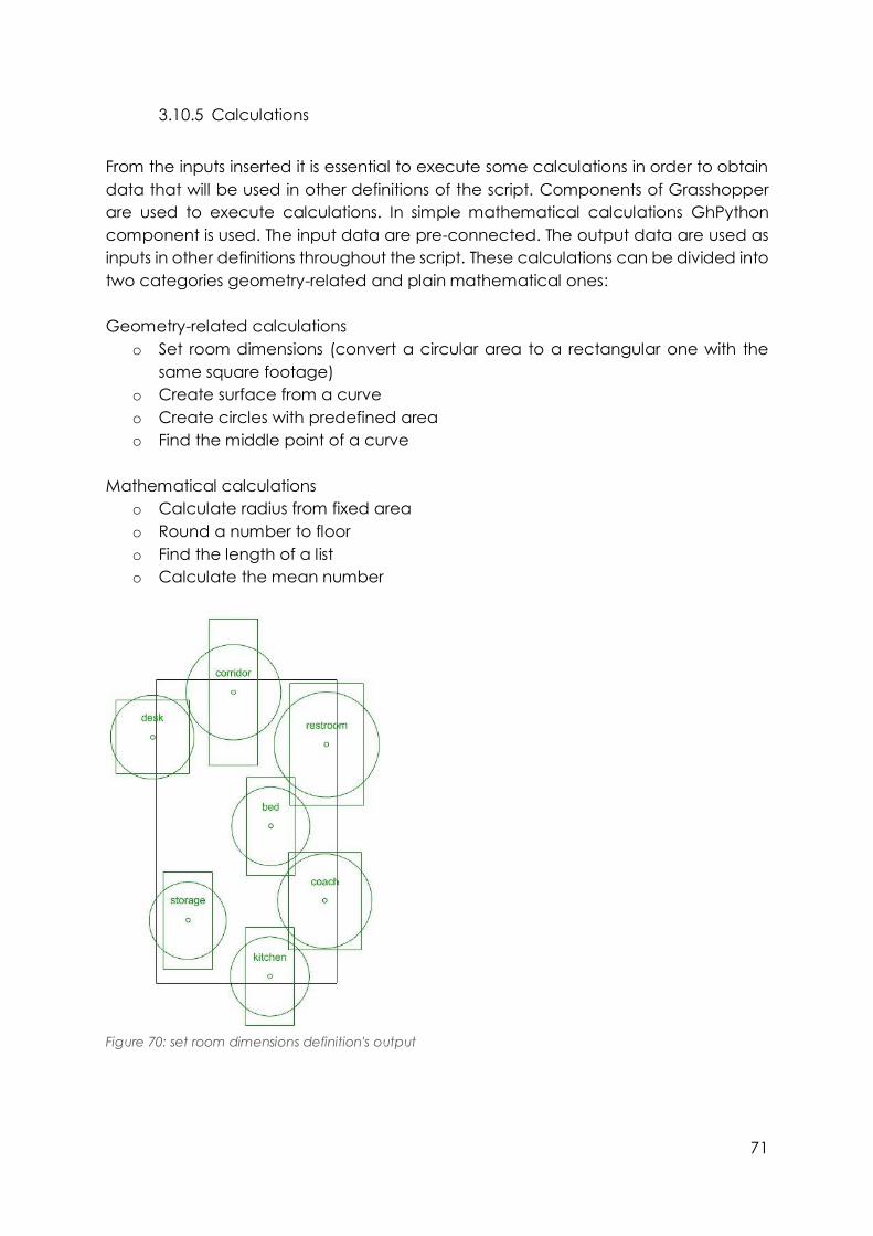
71

3.10.5 Calculations

From the inputs inserted it is essential to execute some calculations in order to obtain

data that will be used in other definitions of the script. Components of Grasshopper

are used to execute calculations. In simple mathematical calculations GhPython

component is used. The input data are pre-connected. The output data are used as

inputs in other definitions throughout the script. These calculations can be divided into

two categories geometry-related and plain mathematical ones:

Geometry-related calculations

o Set room dimensions (convert a circular area to a rectangular one with the

same square footage)

o Create surface from a curve

o Create circles with predefined area

o Find the middle point of a curve

Mathematical calculations

o Calculate radius from fixed area

o Round a number to floor

o Find the length of a list

o Calculate the mean number

Figure 70: set room dimensions definition's output

72

3.11 Layout development

From bubble diagram to layout

In order to design a proper layout based on the bubble diagram produced by the

tool the following 7-steps algorithm was developed and executed manually in

Rhinoceros software:

1. The starting point is the bubble diagram (this is the output of the tool)

2. Then the bubbles (circles) are converted into rectangles. To set dimensions with

the same area a definition called “Set room dimensions” was developed and

can be found in appendix A.

3. Next step is to add existing external elements such as walls, main entrance and

windows.

4. Some of the rooms require walls (eg restroom) and other do not (eg corridor).

In this step it is determined which rooms require what amount of walls (0-4).

5. Afterwards the rooms with largest number of rooms (4) are move towards the

inner corners of the boundary, so as to cast as much less shadow as possible to

the rest rooms.

6. The rest rooms are placed beneath the closed rooms (rooms with 4 walls)

7. Last step is to add furniture. As discussed in paragraph “System of modules” a

series of experiments were made for each unit based on a system of a square

model of 0.50x0.50m.

Unit A – studio for one student

Figure 71: Step 1 - Bubble diagram (output of

tool)

Figure 72: Step 2 - Convert bubbles to

rectangles with the same area and set

rooms' dimensions

73

Figure 73: Step 3 - Add exterior elements

(walls, entrance, windows)

Figure 74: Step 4 - add necessary interior

walls of the rooms

Figure 76: Step 5& 6 - Move rooms

with 4 walls towards the inner corners

of the boundaries so as not to cast

much shadow to the rest rooms. Rest

rooms are placed beneath them

Figure 75: Step 7 - Add furniture. The

furniture configuration emerged after a series of experimentations based

on the system of modules with typical

furniture (see paragraph System of

modules)

74

The same process was repeated for the rest unit types. Below are present the first

and final stages only:

Unit B – shared apartment for two people

Figure 78: Unit B - Bubble diagram

Figure 77: Final layout of unit A (studio for student) with

recommended furniture

arrangement and balcony

75

Figure 79: Unit B - Final layout

Unit C – common facilities for student housing

Figure 80: Unit C - Bubble diagram

Figure 81: Unit C - Final layout

76

Unit D – common facilities for student housing at ground floor

Figure 82: Unit D - Bubble diagram

Figure 83: Unit D - Final layout

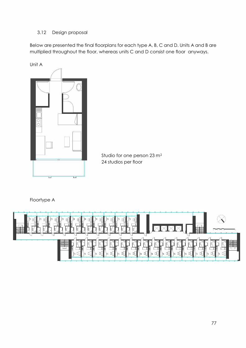
77

3.12 Design proposal

Below are presented the final floorplans for each type A, B, C and D. Units A and B are

multiplied throughout the floor, whereas units C and D consist one floor anyways.

Unit A

Floortype A

Studio for one person 23 m2

24 studios per floor

78

Unit B

Floortype B

Floortype C

Shared apartment for two

people 49 m2

12 apartments per floor

79

Floortype D

80

81

4 Evaluation

82

Evaluation is a critical part of this research, since these kind of tools are relative new

to architectural workflow and are still under development. For this reason, any

contribution is welcome. The evaluation concerns the evaluation of the tool

(computational part) as well as the evaluation of the design development (manual

part).

4.1 Evaluation of the tool

In order to validate the results (both for proximity and illuminance) two checks can be

carried out using Grasshopper. The first one checks whether the proximity

requirements set at the beginning are met, meaning if the rooms with strong

connections are placed very close to each other and with medium connections are

placed relatively close, etc. The second check calculates the mean illuminance of

each room and informs the user about the result (if it matches with the illuminance

category requested). In this way the user can easily assess whether the illuminance

requirements of each room are met or not. In case one or more requirements are not

met the user has to adjust the requirements set in the inputs section. A good idea

would be to check also if the requirements set are reasonable. In any case the results

are indicative so the user should evaluate himself/herself whether any modifications

are needed.

Proximity check

In order to check whether the proximity requirements are met the distance between

the points is calculated first. Then the sum of the corresponding radii is calculated.

Afterwards, a tolerance factor is created for the three different proximity connection

types (strong, medium, weak). The definition checks if the ratio of the distance to the

sum of the radii is smaller than the tolerance factor. If it is then the proximity

requirement is met. The detailed definitions are presented in appendix A.

o Distance calculation 𝑑𝑖𝑗 and sum of radii calculation 𝑟𝑖 + 𝑟𝑗

o Ratio calculation 𝑑𝑖𝑗

𝑟𝑖+ 𝑟𝑗

o Ratio check

|𝑑𝑖𝑗|

𝑟𝑖 + 𝑟𝑗 < 𝑡 , 𝑓𝑜𝑟 𝑡 = 1.5

Below some recommendations for the tolerance factor are presented:

Category

Prox. factor Connection Tolerance

1 0.3 Weak 4* 𝑡

2 0.6 Medium 2 * 𝑡

3 0.9 Strong 𝑡

83

Figure 85: calculate distance between centroids and check them

according to the sm of their radii

Illuminance check

A way to check whether the rooms are placed in positions that fulfill the illuminance

requirements is by finding which test points are included in each circle and then

calculate the mean illuminance value of these points. The detailed definitions can be

found in appendix A. An overview of the definition is presented below:

o First decide which rooms need to be checked

o Find which test points are included in the circle

o Find the index of these test points

o Calculate the mean value in lux of the test points included

𝑚𝑒𝑎𝑛 = ∑ 𝑙𝑢𝑥

𝑛

o Put all lux values in a list (display bubble diagram with illuminance values)

Figure 84: relationship between

distance and radii according to

different proximity connection

types

84

Below the illuminance categories as set in “Illuminance requirements” paragraph

are presented:

Category

Min lux Max lux

1 100 300

2 300 500

3 500 max

Figure 87: all test points with their

corresponding illuminance values in

lux

Figure 86: test points included in circles

85

4.2 Evaluation of the design development

Comparison with conventional method

In the following figure P. MacLeamy compares a preferred design process (in his case

an integrated) with a conventional one through the design stages. For the purposes

of this thesis the preferred integrated design process is a computational process that

integrates proximity and daylight criteria. As we can see in the figure the design stages

that require more effort are the three first ones. In particular, schematic design and

design development require the highest effort and the cost of any changes is smaller

in comparison to conventional design process. In this dissertation the schematic

design was managed to be developed computationally, whereas the design

development phase was developed manually. By following the computational

approach the hardest part is done early, when the cost of modifications is low and all

rest phases require less effort, since most decisions were made from the beginning.

[51]

The phases that were included in this project were:

Pre-design (inputs)

building’s info

rooms

areas

Figure 88: Patrick MacLeamy curve [51]

86

Schematic design (bubble diagram)

proximity requirements

illuminance requirements

prioritization of connections

rooms’ positions based on requirements

Design development (layout)

interior walls

rooms’ dimensions

furniture

Before developing the tool the layouts for floortypes A, B and C were made without

using Cochleas at all. It is interesting to make a comparison between the completely

manual layouts and the ones generated with Cochleas in respect to proximity and

illuminance. As far as time and effort concerns it took almost 8 hours (one working

day) to complete a floorplan following the conventional design method taught in

architecture school, whereas it took 3 hours only to complete the same floorplan when

following Cochleas. The reasons behind it is that the script in Grasshopper is structured

clear enough so as to allow modifications easily and also the user has to make clear

decisions such as proximity connections between rooms at the very beginning. This

reduces the range of options that usually the architect spends much time

experimenting with. As for the bubble diagram itself, the one produced manually is

slightly better, but the one produced by the tool is very similar when rational inputs

used. The final design result, the layout, is clearly of a higher quality when designed

manually, which makes absolute sense since the architect takes many more than two

design criteria into consideration (even subconsciously). The table below shows the

result from the comparison made between conventional and proposed methodology

in this thesis:

criteria

conventional proposed

time

effort

3x less

decision making prioritization

bubble diagram slightly better

layout better

87

Unit A

Figure 89: Layout of unit A designed completely manually

Figure 90: Layout of unit A designed partly computationally

Unit B

Figure 91: Layout of unit B designed completely

manually

Figure 92: Layout of unit B designed partly computationally

88

Floortype C

Figure 94: Layout of unit C designed completely manually

Figure 93: Layout of unit C designed partly computationally

89

5 Conclusions

90

In order for the tool to be useful to architects it has to be assured that it can be easily

understood and customized by them. Customizability and repeatability conclusions

are presented below:

Customizability

One of the main reasons why Grasshopper was chosen as the environment to apply

the methodology is because it was designed to build generative algorithms. Every

numerical input is inserted in the form of sliders so that the user can quickly customize

the values. By designing parametrically all changes in values and geometry can be

done much quicker than using conventional design software (such as Rhinoceros

alone).

Repeatability

This research is documented in detail in the present report so that it can be repeated

and improved by future researchers. The full Grasshopper script is presented in

appendix A. The tool includes explanatory tags so as to guide the user through it.

By evaluating the tool (see chapter 4 “Evaluation”) it can be concluded that the

proposed tool succeeds to do what it is asked; to produce the optimal configuration

regarding proximity and illuminance results. The framework used, spring network

simulation, was successful since the proximity and illuminance checks within the tool

are performing as expected in most cases.

Optimal configuration regarding proximity & illuminance

The spring system approach proved to be successful for dealing with connectivity

requirements. The hierarchy of requirements can be expressed by using different

stiffness values and in this way allow the user to have more control over the resulting

bubble diagram. Illuminance requirements can be translated into proximity

requirements if rooms are connected with points on the floor that have the ideal

illuminance values. The tool handled both requirements as expected.

Computational tools

Existing computational tools (Rhinoceros, Grasshopper and their plugins) are very

useful for architects because they are relatively easy to grasp and intuitive. An

architect with minimum knowledge of mathematics and physics could understand

every step of the process. The computation time of calculations is very low, since no

weird geometry is involved and the illuminance analysis is performed for one day of

the year only. However existing plugins for Grasshopper, such as KangarooPhysics,

have limited capacities and the user cannot have a full control over the procedures,

as it happened with the spring system. In this spectrum it is best to design the definition

from scratch in a programming language (such as the force directed graph drawing

algorithm).

Converting an existing layout into a residential one

91

The extent to which it is possible to convert an existing layout into a residential one

depends on the level of complexity desired. From this research it is clear that a

residential layout requires way more than two design criteria (proximity and

illuminance in this case). In order to design a bubble diagram that can be transformed

into a proper layout more parameters have to be taken into consideration (privacy,

safety, view, noise, circulation). The resulting bubble diagram can be used as

guidelines for the designer to design a high-quality layout. The bubble diagram

consists a very important step for interior space planning.

Further recommendations

The tool has a strong potential to include more climate aspects to the optimization

such as thermal, noise, drift, etc. The same framework could be used and these extra

requirements could be added as extra connections (springs). Apart from this, it could

be applied not only for residences, but also in other uses such as offices, shops. An

attempt is made in this thesis in units C and D that accommodate communal facilities.

Moreover, the tool could take into consideration z axis and apply it in two-stories

apartments. An interesting experiment would be to use the tool to design a layout

from scratch (instead of repurposing an existing one) or try irregular shapes as

building’s boundaries and/ or as proposed rooms’ geometry. It can be definitely

improved as far as computational efficiency concerns by automating manual tasks

(during design process) and by structuring the script better (avoiding loops and

unnecessary commands). The environment chosen for application (Grasshopper) was

not the best one, since it still a project under development, it is limited in capabilities

and it not open source. Therefore, coding in a programming language (such as

python) would be much more suitable for this project. Hence this is the area to further

improve. So next step until graduation is to translate as many grasshopper nodes as

possible to python nodes. The ultimate goal would be to bypass Kangaroo completely

and perform dynamic relaxation with python instead.

92

Reflection

The ultimate goal of the research is to explore ways of how to rationalize and

formulate mathematically a configurational design problem. This design problem

refers to how to arrange a residential program into an existing building not only in

terms of available space but also in relation to two design criteria: proximity and

illuminance.

The initial approach aimed to formulate the problem as abstract as possible using

mathematical procedures. The procedure that seemed the most promising was to

understand what spectral graph theory is and how it is possible to formulate the above

mentioned configurational problem by using principles of graph theory. In a later

stage these principles could be (ideally) written in a programming language (such as

Python or C#) but this was not feasible in this case because of lack of programming

skills from the author. So the most feasible scenario seemed to be to try implementing

the graph theory principles needed into the workflow of Grasshopper environment.

However, the initial approach was abandoned after the second presentation (P2)

because it was realized that it was not possible for the author to gain knowledge in

advanced mathematics topics of discrete mathematics (spectral graph theory,

topology) and rest topics relative to calculus and linear algebra needed in such a

short period of time so as to develop a methodology on how to apply these methods

to the design assignment. Under these circumstances the approach of a fully

automated methodology - although well-grounded and challenging - would be way

beyond the MSc graduation thesis purposes of a Building Technology student.

The next step was to find another approach to achieve the ultimate goal of the

research. According to research methodology set at the beginning of the research,

stages 1 (research framework) and 2 (theoretical background) had to be repeated.

After completing the new literature review, generative design using existing

computational tools seemed to be the most promising approach. The visual

programming environment for this purpose was chosen to be Grasshopper, because

of its popularity among the architectural community and its ability to support

generative algorithms. The proposed approach is a systematic approach in which it

is investigated until what point it is possible to automate a part of the design process

in primary design stage according to the user’s wishes (manual input) in respect to

rooms’ connectivity (proximity of rooms) and daylight criteria (illuminance) using

computational methods.

The research methodology was set at the very beginning of the research (P1) and was

followed until the completion of the research. It can be summarized in the following

stages:

Research framework

Theoretical background

Tool development

93

Evaluation

Conclusions

The first two steps were repeated after P2 retake and resulted in the new approach

which is dynamic relaxation. During the tool development phase the specifications

and assumptions were set so as to structure the tool. In the beginning, the main

skeleton of the tool was defined by relative research, but it was not fully developed

until it was applied in the case study. By following the proposed methodology it was

possible to produce and evaluate the outputs. If the result was not satisfactory the

process was repeated but this time the chosen parameters were adjusted to see

which parameter had the greatest impact. By trials and relative research in literature

the tool started to take its final form. The evaluation step was necessary so as to check

how the tool performs in future applications. The last step includes the discussion upon

the results, the conclusions drawn from the discussions and recommendations for the

tool’s improvement.

As far as society concerns, renovation was and still is an import design assignment,

especially in countries where its available to build area is limited. Converting existing

buildings into residences is a way to tackle the housing problem many people (locals

and expats) from all over the world face. In a professional point of view, finding a way

to systemize the renovation design process could have a great impact on the way

architects would approach a renovation project since the very beginning. As soon as

they have an initial design idea by following the suggested methodology it would be

possible to insert the necessary data and produce the schematic residential layout

based on the two –most important according to the author- design criteria: proximity

and daylight. One of the main advantages of computational applications is that they

can handle a respectable amount of data simultaneously. This means that many

levels of complexity can be added to the tool and in that way help the architect find

the optimum layout. This could speed up the design process and also produce non-

conventional but still functional layouts.

The current graduation project is directly related to MSc Architecture, Urbanism and

Building Sciences and the Building Technology track. Firstly, the computational

methods proposed are intended to be applied in existing buildings, in real life

scenarios, which is what architecture and building sciences is about. The case studies

selected empower the practicality and the usefulness of the tool. The intention to

contribute to systemize the renovation design process is an architectural intention

interwoven with sustainability, that is one of the main aspects of Building Technology.

Building Technology is also the field where architects are more oriented towards

engineering. Mathematics and physics is some of the fundamental subjects of an

engineer. Engineering is also about improving existing methods as well as inventing

new ones. In this dissertation the innovation lies in developing a methodology on how

to systemize a renovation design project using principles of computer science,

mathematics and physics.

94

The peculiarity of this graduation topic, as well as most topics of generative design, is

that the methodology followed during the research is in fact the research product. In

this report is presented not only the final methodology that led to the desired results,

but also the process of exploration; all trials and the logic behind them. This is also the

main teaching objective of this research: to learn from successes as well as from

failures.

To sum up, the proposed tool succeeds to do what it is asked for; namely to produce

the optimal configuration regarding proximity and illuminance results. The framework

used, dynamic relaxation was successful as my main mentor predicted. The tool has

a lot of potential to be enlarged and include more climate aspects to the optimization

such as thermal, noise, drift, etc. The same framework could be used and add these

requirements as extra connections (springs). However, the environment chosen

(Grasshopper) was not the ideal choice, because it still a project under development,

is limited in capabilities and it not open source. Therefore, coding in a programming

language (such as Python) would be the ideal environment for this project.

95

List of figures

Figure 1: Research scope ................................................................................................... 8

Figure 2: graph representing the problem in a simple form where a, b, c the initial

room positions, a’, b’, c’ the ideal illuminance positions and af , bf , cf the final room

positions ............................................................................................................................. 10

Figure 3: adjacency matrix for proximity connections .................................................. 10

Figure 4: adjacency matrix for illuminance connections .............................................. 10

Figure 5: Problem statement Step 1: empty existing building, Step 2: calculate

illuminance values of test points on grid Step 3: set room’ centroids and their

proximity requirements as line segments, Step 4: final configuration of rooms based

on proximity and illuminance requirements set are shown as bubble diagram, Step 5:

final layout based on the bubble diagram .................................................................... 11

Figure 6: Research methodology workflow .................................................................... 15

Figure 7: generative design flowchart by H. Bohnacker [23] ........................................ 18

Figure 8: the graph of gradient descent algorithm in respect to cost and weight [26]

........................................................................................................................................... 20

Figure 9: the three possible results of gradient descent: local minimum, global

minimum and plateau [26] .............................................................................................. 20

Figure 10: Schematic explanation of Hooke's law[28] ................................................... 22

Figure 11: Force towards displacement diagram [29]................................................... 23

Figure 12: graph representing the problem in a simple form where a, b, c the initial

room positions, a’, b’, c’ the ideal illuminance positions and af , bf , cf the final room

positions ............................................................................................................................. 28

Figure 13: Different analysis diagrams for one apartment floor plan [34] ................... 31

Figure 14: links of rooms with dense packing and respective door placement [35] .. 32

Figure 15: alterations of rooms' arrangement together with possible visibility offered

by the doors [35] ............................................................................................................... 32

Figure 16: input: geometry as circles and height, output: pixelated, extruded and

arranged volumes [36] ..................................................................................................... 33

Figure 17: The simulation process: a) The initial position of spaces showing volumes

and springs action directions. b) Spaces behavior under spring forces. c) First

simulation result. d) Second simulation result. [37] ......................................................... 34

Figure 18: Relationship chart [38] .................................................................................... 35

Figure 19: Space relationship [38] ................................................................................... 35

Figure 20: An existing floor plan with a spatial subdivision and pre-matches; Bubble

diagram of functions (with relative sizes); The initial spectral matching (normalized-

Laplacian matrix and UPGMC, Renormalized); Improved matching through a hill

climber. [39] ...................................................................................................................... 36

Figure 21: Photo of EEMC in Delft (from ground level) [41] ........................................... 38

Figure 22: Photo of EEMC in Delft (aerial view) [42] ....................................................... 39

Figure 23: Screenshot from google maps indicating the location of EEMC [45] ......... 40

Figure 24: Orientation of EEMC [46]................................................................................. 40

Figure 25: Direct sunlight analysis of EEMC for July [46] ................................................. 41

96

Figure 26: Dominant wind analysis for EEMC [46] ........................................................... 41

Figure 27: Ground floor layout of EEMC [47] .................................................................. 42

Figure 28: Layout of a typical floor of the tower of EEMC [47]...................................... 43

Figure 29: perspective view of the main corridor at the tower (existing situation) [46]

........................................................................................................................................... 43

Figure 30: schematic representation of the structural system a typical tower’s floor

[46] ..................................................................................................................................... 44

Figure 31: photo of the interior of the main corridor at the 21st floor [48] ................... 44

Figure 32: photo of hall L located at the ground floor [49] ........................................... 44

Figure 33: Table with units and residents numbers ......................................................... 45

Figure 34: Vertical arrangements of uses ........................................................................ 46

Figure 35: Area of interest (in pink) in a typical floor of the tower ................................ 46

Figure 36: Program of requirements for unit A (studios) ................................................. 47

Figure 37: Program of requirements for unit C (common facilities) .............................. 47

Figure 38: Program of requirements for unit B (shared apartments) ............................ 47

Figure 39:Program of requirements for unit D (common facilities at ground floor) ..... 47

Figure 40: configuration exploration based on the modules and minimum furniture

required per room for type A ........................................................................................... 49

Figure 41: REL-chart for studios (type A).......................................................................... 52

Figure 42: REL-chart for shared apartments (type B) ..................................................... 52

Figure 43: REL-chart for common facilities (type C) ....................................................... 53

Figure 44: REL-chart for common facilities at ground floor (type D) ............................ 53

Figure 45: Recommendations of daylight provision [50] ............................................... 54

Figure 46: Minimum recommended lighting levels for residential spaces [51] ............ 55

Figure 47: illuminance categories with their respective minimum and target lux values

........................................................................................................................................... 56

Figure 48: illuminance requirements for studios .............................................................. 56

Figure 49: illuminance requirements for shared apartments ......................................... 56

Figure 50: illuminance requirements for common facilities ........................................... 57

Figure 51: illuminance requirements for common facilities at ground floor................. 57

Figure 52: colour coding rule ........................................................................................... 58

Figure 53: Flowchart of the tool ....................................................................................... 59

Figure 54: some of the inputs as seen in grasshopper (entrance position, boundary,

rooms’ centroids) .............................................................................................................. 62

Figure 55: proximity requirements (strong connections in blue, medium connections

in red)................................................................................................................................. 63

Figure 56: Hierarchy of proximity connections ............................................................... 63

Figure 57: legend of the illuminance analysis ................................................................. 64

Figure 58: all test point with their corresponding lux values .......................................... 64

Figure 59: points in black: centroids of rooms, points in green: test points, lines:

illuminance connections .................................................................................................. 64

Figure 60: illuminance categories with their respective minimum and target lux values

........................................................................................................................................... 64

Figure 61: colored mesh result of illuminance analysis .................................................. 66

Figure 62: all test point with their corresponding lux values .......................................... 66

97

Figure 63: system's input ................................................................................................... 68

Figure 64: system's output ................................................................................................ 68

Figure 65: System's output ................................................................................................ 69

Figure 66: New positions of points.................................................................................... 69

Figure 67: Move points with curve collide component of Kangaroo2 ......................... 69

Figure 68: Final bubble diagram with tags ..................................................................... 70

Figure 69: Final bubble diagram with tags and lux values ............................................ 70

Figure 70: colour coding rule ......................................................................................... 101

98

Bibliography

[1] A. Oikonomou, F. Bougiatioti, and P. Georgopoulos, “10th International

Symposium on the Conservation of Monuments in the Mediterranean Basin,”

10th Int. Symp. Conserv. Monum. Mediterr. Basin, no. December, 2018.

[2] “Renovation architecture and design | ArchDaily.” [Online]. Available:

https://www.archdaily.com/search/projects/categories/renovation.

[Accessed: 18-May-2020].

[3] “MVRDV - Transformations.” [Online]. Available:

https://www.mvrdv.nl/themes/7/transformations. [Accessed: 18-May-2020].

[4] Eurostat, Estadísticas de energía renovable. 2018.

[5] “ntorenmarkt houdt wind in de rug Dutch property market in focus Dutch

property market in focus,” 2018.

[6] “Transforming office space into housing | Investing in Dutch housing |

Government.nl.” [Online]. Available:

https://www.government.nl/topics/investing-in-dutch-housing/transforming-

office-space-into-housing. [Accessed: 19-Dec-2019].

[7] “Apartment Renovation | Architect Magazine.” [Online]. Available:

https://www.architectmagazine.com/tag/apartment-renovation. [Accessed:

18-May-2020].

[8] “10 Best renovation projects - Domus.” [Online]. Available:

https://www.domusweb.it/en/news/2018/01/13/best-of-renovation.html.

[Accessed: 18-May-2020].

[9] “Renovation | ArchDaily.” [Online]. Available:

https://www.archdaily.com/category/renovation. [Accessed: 18-May-2020].

[10] “‘Generative Design’ – What’s That? - CIMdata.” [Online]. Available:

https://www.cimdata.com/en/news/item/8402-generative-design-what-s-that.

[Accessed: 28-Mar-2020].

[11] “What is Generative Design | Tools & Software | Autodesk.” [Online].

Available: https://www.autodesk.com/solutions/generative-design.

[Accessed: 18-May-2020].

[12] “What Generative Design Is and Why It’s the Future of Manufacturing | New

Equipment Digest.” [Online]. Available:

https://www.newequipment.com/research-and-

development/article/22059780/what-generative-design-is-and-why-its-the-

future-of-manufacturing. [Accessed: 18-May-2020].

[13] I. Caetano, L. Santos, and A. Leitão, “Computational design in architecture:

Defining parametric, generative, and algorithmic design.”

[14] “The Promise of Generative Design -.” [Online]. Available: https://www.world-

architects.com/en/architecture-news/insight/the-promise-of-generative-

design. [Accessed: 18-May-2020].

[15] “Computational Thinking Benefits Society |.” [Online]. Available:

http://socialissues.cs.toronto.edu/index.html%3Fp=279.html. [Accessed: 18-

May-2020].

[16] “Rhino 6 for Windows and Mac.” [Online]. Available:

https://www.rhino3d.com/. [Accessed: 18-May-2020].

[17] “Grasshopper - New in Rhino 6.” [Online]. Available:

https://www.rhino3d.com/6/new/grasshopper. [Accessed: 18-May-2020].

[18] “Kangaroo3d.” [Online]. Available: http://kangaroo3d.com/. [Accessed: 18-

May-2020].

99

[19] “Ladybug Tools | Home Page.” [Online]. Available:

https://www.ladybug.tools/. [Accessed: 18-May-2020].

[20] “GhPython | Page 6 | Food4Rhino.” [Online]. Available:

https://www.food4rhino.com/app/ghpython?page=5. [Accessed: 23-Jun-

2020].

[21] Mahmoud Mohamed Abdelrahman, “Gh_CPython: CPython plugin for

grasshopper,” 2017.

[22] “The Next Generation of Generative Design - XponentialWorks.” [Online].

Available: https://xponentialworks.com/the-next-generation-of-generative-

design/. [Accessed: 19-May-2020].

[23] “Generative Design Process - Generative design - Wikipedia.” [Online].

Available:

https://en.wikipedia.org/wiki/Generative_design#/media/File:Generative_Desi

gn_Process.png. [Accessed: 19-May-2020].

[24] “Gradient-Based Method - an overview | ScienceDirect Topics.” [Online].

Available: https://www.sciencedirect.com/topics/mathematics/gradient-

based-method. [Accessed: 19-May-2020].

[25] “Gradient Descent Algorithm and Its Variants - Towards Data Science.”

[Online]. Available: https://towardsdatascience.com/gradient-descent-

algorithm-and-its-variants-10f652806a3. [Accessed: 19-May-2020].

[26] “Stochastic vs Batch Gradient Descent - Divakar Kapil - Medium.” [Online].

Available: https://medium.com/@divakar_239/stochastic-vs-batch-gradient-

descent-8820568eada1. [Accessed: 19-May-2020].

[27] P. Nourian and S. Azadi, “Dynamic Relaxation & Force-Directed Graph

Drawing Configraphix: Graph Theoretical Methods for Design and Analysis of

Spatial Configurations View project Design Games View project.”

[28] “Hooke’s law | Description & Equation | Britannica.” [Online]. Available:

https://www.britannica.com/science/Hookes-law. [Accessed: 04-Jul-2020].

[29] “Spring potential energy and Hooke’s law review (article) | Khan Academy.”

[Online]. Available: https://www.khanacademy.org/science/ap-physics-1/ap-

work-and-energy/spring-potential-energy-and-hookes-law-ap/a/spring-force-

and-energy-ap1. [Accessed: 30-Mar-2020].

[30] P. Nourian, “Configraphics Graph Theoretical Methods for Design and Analysis

of Spatial Configurations,” 2016.

[31] “Ladybug Tools · GitHub.” [Online]. Available: https://github.com/ladybug-

tools. [Accessed: 02-Apr-2020].

[32] “Kangaroo Physics | Food4Rhino.” [Online]. Available:

https://www.food4rhino.com/app/kangaroo-physics. [Accessed: 19-May-

2020].

[33] “Kangaroo Manual (Grasshopper version)_edited.”

[34] “How can I understand ‘Strength’ parameter? - Grasshopper / Kangaroo -

McNeel Forum.” [Online]. Available: https://discourse.mcneel.com/t/how-can-

i-understand-strength-parameter/51112. [Accessed: 30-Mar-2020].

[35] S. Schneider, M. Bielik, D. Donath, M. Triemer, J. Tschetwertak, and A. Hollberg,

“Rapid Data Collection using Automated Model Generation and Performance

Evaluation A workflow for morphological studies of apartment floor plans.”

[36] “Floor Plans | Computational Planning Science.” [Online]. Available:

https://entwurfsforschung.de/layout/?fbclid=IwAR31RZ1lj4W-

F3b3SmaWcEk_ZrIvj62AtdVWG5BWlYKNLl05Q85a-bJoEvQ. [Accessed: 04-Feb-

2020].

[37] C. Boon, C. T. Griffin, N. Papaefthimiou, J. Ross, and K. Storey, “Evolutionary

100

parametric analysis for optimizing spatial adjacencies.”

[38] M. Elsayed, O. Tolba, and A. Elantably, “ARCHITECTURAL SPACE PLANNING

USING PARAMETRIC MODELING Egyptian National Housing Project.”

[39] Y. Ojaghi, A. Khademi, N. M. Yusof, N. G. Renani, and S. A. H. B. S. Hassan,

“Production layout optimization for small and medium scale food industry,” in

Procedia CIRP, 2015, vol. 26, pp. 247–251.

[40] R. Schaffranek, “Parallel planning An experimental study in spectral graph

matching.”

[41] “Behoud het markante EWI-gebouw, voor Delft, Nederland en de rest van de

wereld - Petities.nl.” [Online]. Available: https://petities.nl/petitions/behoud-

het-markante-ewi-gebouw-voor-delft-nederland-en-de-rest-van-de-

wereld?locale=nl. [Accessed: 19-May-2020].

[42] “LEGO IDEAS - TU Delft, EWI.” [Online]. Available:

https://ideas.lego.com/projects/89443d4a-1a2f-410a-82a9-7a1e6675413e.

[Accessed: 19-May-2020].

[43] “What of the future of EEMCS?” [Online]. Available:

https://www.delta.tudelft.nl/article/what-future-eemcs. [Accessed: 19-May-

2020].

[44] “Delft Seminars of Building Technology (13‐14Q3) - group 10- User controlled

EWI - YouTube.” [Online]. Available:

https://www.youtube.com/watch?v=5nkDYCzqi7c. [Accessed: 19-May-2020].

[45] “Case study EWI: low rise facade details - AR1A075 - TU Delft - StuDocu.”

[Online]. Available: https://www.studocu.com/hk/document/technische-

universiteit-delft/delft-seminars-on-building-technology/other/case-study-ewi-

low-rise-facade-details/61296/view. [Accessed: 19-May-2020].

[46] “Designet - interieur architectuur voor PMA pensioenfonds voor Apotheken.”

[Online]. Available: https://www.designet.nl/project_TU_Delft.html#.

[Accessed: 19-May-2020].

[47] “TU Delft - Zalenboek - Hall L.” [Online]. Available:

https://educationrooms.tudelft.nl/zaleninfo.php?zid=176. [Accessed: 19-May-

2020].

[48] “Dutch Standards - NEN.” [Online]. Available:

https://www.nen.nl/Standardization/What-is-standardization/Dutch-

Standards.htm. [Accessed: 17-Dec-2019].

[49] “A Room-by-Room Guide for Ergonomic Lighting Levels.” [Online]. Available:

https://www.thoughtco.com/lighting-levels-by-room-1206643. [Accessed: 19-

May-2020].

[50] “honeybee/README.md at master · ladybug-tools/honeybee · GitHub.”

[Online]. Available: https://github.com/ladybug-

tools/honeybee/blob/master/README.md. [Accessed: 19-May-2020].

[51] “The Division 4 Triclinium: Of the MacLeamy Curve, Efficient Design, and

Expensive Money--Or Why Developers are a Breed Apart!” [Online]. Available:

http://division4triclinium.blogspot.com/2013/06/of-macleamy-curve-efficient-

design-and.html. [Accessed: 05-Jul-2020].

[52] “Bestand:TU-Delft-EWI-1.jpg - Wikipedia.” [Online]. Available:

https://nl.wikipedia.org/wiki/Bestand:TU-Delft-EWI-1.jpg. [Accessed: 19-May-

2020].

101

Appendices

Appendix A: Grasshopper script

For documentation purposes the Grasshopper script developed is presented in this

appendix with screenshots. To make things more clear the colour coding rule and

the overview of the script is presented below:

Script overview:

7. INPUTS

Program of requirements

o Room centroids

o Room areas

Building’s info

Proximity requirements

o Proximity connections

o Proximity categorization

Illuminance requirements

o Illuminance categories

o Illuminance connections

8. DAYLIGHT SIMULATION

1 Create apartment box

2 Create zone masses

3 Add glazing

4 Generate test points on grid

5 Generate climate-based sky

6 Grid-based simulation recipe

7 Daylight simulation

8 Legend customization

9 Recolour mesh

10 Save analysis’ files

9. OPTIMAL CONFIGURATION

Proximity

Illuminance

Kangaroo engine

Trails of moving points

Overlap correction

o Circle collision

Figure 95: colour coding rule

102

o Trails of moved circles

10. OUTPUTS

Bubble diagram with lux values

11. CALCULATIONS

Geometry related calculations

o Set room dimensions

o Circles with predefined areas

o Middle point of curve

o Surface from curve

Mathematical calculations

o Radius calculation

o Round number to floor

o Mean of a number

o List length

12. EVALUATION

Proximity results

Illuminance results

o Rooms to be checked

o Test points included in circle

o Finding the index

o Put items in list

103

1. INPUTS

Program of requirements

104

105

Building’s info

106

Proximity requirements

107

108

Illuminance requirements

109

110

2. DAYLIGHT SIMULATION

111

112

113

3. OPTIMAL CONFIGURATION

114

115

116

Overlap correction

117

4. OUTPUTS

5. CALCULATIONS

Geometry related calculations

118

119

Mathematical calculations

2nd way in python (not working)

120

121

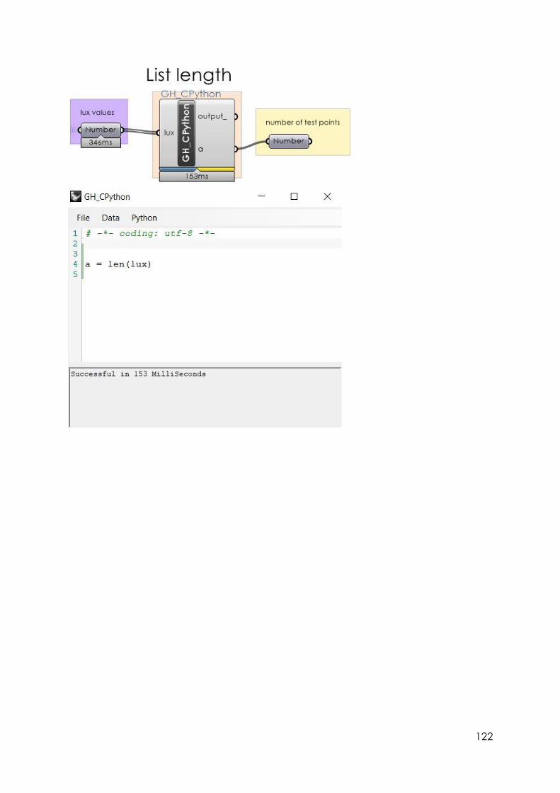
122

123

6. EVALUATION

Proximity results

Ratio calculation

2nd way in python (not working)

124

Ratio check

2nd way in python (not working)

125

Illuminance results

126

2nd way in python (not working)

127

2nd way in python (not working)

128

Appendix B: Pseudocode in Python

With the valuable help of my mentor ir. P. Nourian, the pseudocode of the iterative

process could be structured like this:

Epsilon=0.00001

repulsionStiffness=1

continuance_condition=True

iterationCount=0

While (continuance_condition=true ‘and’ iteration_count<max_iteration):

for i in range(0,n):

o if not i is in fixedVertexIndices:

sumAttractionForces=rg.Vector3d(0,0,0)

sumRepulsionForces=rg.Vector3d(0,0,0)

for j in range(0,n):

edgeKey=(i, j)

(length, stiffness, force, r_i, r_j,v_i,v_j)=edges[edgeKey]

v_i=vertices[i]

v_j=vertices[j]

d_ij=v_j-v_i

r_i=radii[i]

r_j=radii[j]

k_ij=K[i,j]

f_ij=k_ij*d_ij

converged=((abs(d_ij.length/(r_i+r_j) -1))<epsilon)

continuance_condition= continuance_condition and !converged

sumAttractionForces=force+sumAttractionForces

if (length<(r_i+r_j)):

....1. repulsionForce=-1*length*repulsionStiffness

....2. sumRepulsionForces= sumRepulsionForces+repulsionForce

resultantForce = sumAttractionForces+ sumRepulsionForces

vertex=vertices[i] vertex=vertex+0.1* resultantForce

iterationCount=ierationCount+1

129

130