PROCESS TO CONVERT AN EXISTING BUILDING INTO ZERO ...
101
T.E.I of Western Greece Page | 1 MASTERS PROJECT THESIS ON PROCESS TO CONVERT AN EXISTING BUILDING INTO ZERO ENERGY BUILDING(ZEB) IN 3 CITIES (LONDON,PATRAS AND CHENNAI) : COMPARATIVE RESULTS BY KISHORE KUMAR SRIDHARAN (A.M – 35) (2014-2016) UNDER THE ESTEEMED GUIDANCE OF PROF. SOCRATES KAPLANIS, BSc, MSc, PhD, D.H.C.Brasov University Head of the Renewable Energy Systems (RES) Laboratory .
-
Upload
khangminh22 -
Category
Documents
-
view
3 -
download
0
Transcript of PROCESS TO CONVERT AN EXISTING BUILDING INTO ZERO ...

T.E.I of Western Greece
Page | 1
MASTERS PROJECT THESIS ON
PROCESS TO CONVERT AN EXISTING BUILDING INTO
ZERO ENERGY BUILDING(ZEB) IN 3 CITIES
(LONDON,PATRAS AND CHENNAI) : COMPARATIVE
RESULTS
BY
KISHORE KUMAR SRIDHARAN (A.M – 35)
(2014-2016)
UNDER THE ESTEEMED GUIDANCE OF
PROF. SOCRATES KAPLANIS, BSc, MSc, PhD, D.H.C.Brasov University
Head of the Renewable Energy Systems (RES) Laboratory .

T.E.I of Western Greece
Abstract
This dissertation details the process for converting an existing building into a Zero Energy
Building(ZEB) in 3 major cities namely London,Patras and Chennai located in the United
Kingdom, Greece and India respectively.Initially,the overall Heat losses coefficient (UA)b is
determined for the building in each one of the cities .Subsequently,the thermal Loads
comprising Heating (Space Heating,Domestic hot water and Heat losses)and the Cooling
loads for the building are determined through appropriate equations for the seasonal
months(Jan,Apr,Jul,Oct). In addition,the electric loads of the building in the 3 cities are
calculated.By the use of passive solar techniques which considers the solar gain through the
windows , the thermal demand(Space Heating Load) of the building is reduced .To satisfy the
thermal load demand through renewables ,solar collectors are considered and a daily hourly
simulation is performed to calculate the collector output following which the area of the
collectors required for different fraction of the loads is determined.The Heat Pump is sized
for satisfying the cooling demand in Chennai.A stand alone PV system is designed to meet
the electric Loads .In addition,an important comparison is made between the 2 approaches
used to calculate the Space Heating Load and the 2 approaches used for the sizing of the
stand alone PV in the thesis.Finally,the dissertation concludes by performing an economic
analysis to calculate the Net Present Value(NPV)and the Internal Rate of Return(IRR) for
different fraction of thermal needs by Solar Collector to determine the scenario with most
economic feasibility.
Page | 2

T.E.I of Western Greece
Page | 3
Contents
.................................................................................................................................. 7
1.1 Zero Energy Buildings (Definitions) ............................................................................... 7
1.2 Introduction ................................................................................................................. 8
................................................................................................................................ 11
................................................................................................................................ 18
3.1 Climatic Conditions (India) ........................................................................................ 18
3.1.1 Solar Radiation and Temperature Profiles (Chennai) ................................................ 19
3.2 Climatic Conditions in England ................................................................................. 20
3.2.1 Solar Radiation and Temperature Profiles (London) ................................................. 21
3.3 Climatic Conditions in Greece ................................................................................... 22
3.3.1 Solar Radiation and Temperature Profiles ................................................................. 23
................................................................................................................................ 25
4.1 Properties to consider in the selection of Insulation materials ....................................... 25
4.2 Building Regulations and the EU .................................................................................. 26
4.2.1 Building Regulation (Greece) ..................................................................................... 27
4.2.2 Building Regulation(India) ......................................................................................... 27
................................................................................................................................ 29
5.1 Determination of Thermal Heat losses Coefficient (UA)b of a Building ....................... 29
5.1.1 Calculation of (UA)b of the Building ....................................................................... 32
5.2 Heating and Cooling Degree Days for 3 cities ............................................................... 35
5.3 Calculation of Solar Gain for the Windows in London,January ................................... 37
5.4 Calculation of Space Heating, Cooling and other thermal Loads .................................. 42
5.4.1 Space Heating & other Thermal Loads for London,Patras .................................... 44
5.4.2 Space Heating Load calculation (Alternative approach by using hourly temperature
data) ...................................................................................................................................... 45
5.4.3 Calculation of Cooling Loads for Chennai .............................................................. 47
5.5 Electric Loads of the building in 3 cities.................................................................... 52
................................................................................................................................ 55
6.1 Calculation of Output of the Solar Collector ................................................................ 55
6.2 Cooling Equipment selection for Cooling Loads(Chennai) .......................................... 59
6.3 Sizing of Stand-alone PV for meeting the Electric Loads ............................................ 63
6.4 Sizing of Stand-alone PV using a stochastic approach ................................................. 73

T.E.I of Western Greece
Page | 4
6.4.1 Simulation Methodology ........................................................................................... 74
................................................................................................................................ 79
................................................................................................................................ 85
8.1 Comparison of Space Heating Load between the 2 approaches ............................... 85
8.2 Comparison of the sizing of stand-alone PV between the 2 approaches .................. 86
................................................................................................................................ 87
List of Tables
Table 3-1 : Classification of Climatic Zones ........................................................................... 19
Table 4-1: Maximum U Values(W/m2K) ................................................................................ 26
Table 4-2:The elemental U-value(W/m2K) requirements for new build under ...................... 26
Table 4-3:Minimum U values(W/m2K) according to the new and previous regulations ........ 27
Table 4-4:ASHRAE Building Envelope Requirements ........................................................... 28
Table 4-5:Roof assembly U-factor and Insulation R-value Requirements .............................. 28
Table 4-6:Opaque Wall assembly U-factor and Insulation R-value Requirements ................. 28
Table 5-1: Building Parameters ............................................................................................... 32
Table 5-2:Building Elements ................................................................................................... 32
Table 5-3: Building Elements Thickness and Thermal Conductivity ...................................... 32
Table 5-4:(UA)b of the building (London) ............................................................................... 33
Table 5-5: (UA)b of the building(Patras) ................................................................................. 34
Table 5-6:(UA)b of the building (Chennai) .............................................................................. 35
Table 5-7: Heating and Cooling Degree Days(Chennai) ......................................................... 35
Table 5-8: Heating /Cooling Degree Days London ................................................................. 36
Table 5-9:Heating /Cooling Degree Days Patras ..................................................................... 36
Table 5-10: Solar Radiation Intensity, London on representative day for January ................. 37
Table 5-11:Fraction of Diffuse given by Orgill and Hollands Model ..................................... 38
Table 5-12: Hourly Beam and Diffuse Radiation .................................................................... 39
Table 5-13: Properties of Glass Windows ............................................................................... 39
Table 5-14: Transmission Coefficient of Glass ....................................................................... 40
Table 5-15: Hourly Solar Gain for building in London,January ............................................. 41
Table 5-16: Solar gain (daily&monthly)for 3 cities ................................................................ 42
T.E.I of Western Greece
Page | 5
Table 5-17: Mains Cold Water Temperature in 3 cities (For Patras taken from TECSOL and
assumed values for other 2 cities) ............................................................................................ 42
Table 5-18: Thermal Loads for the Building in London and Patras ........................................ 44
Table 5-19:Hourly Temperature values + 3 days representative day for London ,
January(n=17) .......................................................................................................................... 45
Table 5-20:Space Heating Load considering hourly values of temperature London(January)46
Table 6-1:Properties of Flat plate solar Collector .................................................................... 55
Table 6-2: Monthly Output of the Solar Collector (London) .................................................. 57
Table 6-3: Monthly Output of the Solar Collector(Patras) ...................................................... 58
Table 6-4:Collector Area and quantity of Collectors(London & Patras) ................................. 58
Table 6-5: TD Value (from Manual S) .................................................................................... 60
Table 6-6: Expanded Performance Data for Cooling with an Air-Cooled Condenser or Heat
Pump (Source :Manual S) ........................................................................................................ 62
Table 6-7: Irradiation on the Horizontal and Optimal inclination angle for Chennai ............. 64
Table 6-8: Irradiation at the Optimal inclination angle for Chennai ....................................... 65
Table 6-9:Annual Stand alone PV performance with days of autonomy 3 ............................. 68
Table 6-10:Annual Stand alone PV performance with days of autonomy 2 ........................... 69
Table 6-11: Stand alone PV system chennai design details ..................................................... 72
Table 6-12: Stand alone PV system(London) design details ................................................... 72
Table 6-13:Stand alone PV system(Patras) design details ....................................................... 72
Table 6-14:PV Simulation values on a typical day(n=11) for Peak Power Pm = 1.5 kW and
Battery Capacity ,CL = 186Ah // London(December) ............................................................. 76
Table 7-1: Different fractions of thermal loads by solar collector ........................................... 79
Table 7-2:Costs for Solar Thermal Technologies .................................................................... 80
Table 7-3: Oil Consumption in litres to cover 100%Thermal Loads ....................................... 81
Table 7-4: NPV & IRR table for Solar Collector,Patras .......................................................... 83
Table 7-5: NPV & IRR table for Solar Collector, LondonTable 7-4: NPV & IRR table for
Solar Collector,Patras .............................................................................................................. 83
Table 7-5: NPV & IRR table for Solar Collector, London ...................................................... 84
Table 7-5: NPV & IRR table for Solar Collector, London ...................................................... 84

T.E.I of Western Greece
Page | 6
List of Figures
Figure 1-1: Breakdown of EU residential electricity consumption,2007 .................................. 8
Figure 1-2:World-wide locations of nZEB ................................................................................ 9
Figure 1-3:The monitoring and infrastructure of a ZEB/PEB system ..................................... 10
Figure 2-1: Site Boundary of Energy Transfer for Zero Energy Accounting .......................... 12
Figure 2-2:Overview of possible renewable supply options.................................................... 13
Figure 2-3:The components of a ZEB/PEB architecture during real-time operation .............. 14
Figure 2-4 :Scheme of grid-connected renewable electricity system ...................................... 15
Figure 2-5: Principle diagram of the PV-SolarThermal-HeatPump ZEB ................................ 16
Figure 2-6: Principle diagram of the Wind-SolarThermal-HeatPump ZEB ............................ 16
Figure 3-1: Map of India showing Climatic Zones(Based upon survey of India outline map
printed in 1993) ........................................................................................................................ 18
Figure 3-2: Horizontal Irradiation(average daily)for Chennai ................................................. 19
Figure 3-3:Hourly Ambient Temperature,Ta profiles on the Representative days of Seasonal
months,Chennai ....................................................................................................................... 20
Figure 3-4:Horizontal Irradiation(average daily)for London .................................................. 21
Figure 3-5:Hourly Ambient Temperature,Ta profiles on the Representative days of Seasonal
months,London ........................................................................................................................ 22
Figure 5-1: Effect of insulation thickness on U-value ............................................................. 30
Figure 5-2: Plots of Thermals loads in 3 cities ........................................................................ 52
Figure 5-3: Electric Loads of 3 cities - Bar chart..................................................................... 54
Figure 6-1: Cooling equipment selection steps ........................................................................ 59
Figure 6-2: Wet-bulb temperature on sea-level psychometric chart ........................................ 62
Figure 6-3:Irradiance profile(daily)for Chennai ...................................................................... 67
Figure 6-4:Hourly Consumption profile of the selected Loads ............................................... 71
Figure 7-1: Installed Costs for Solar Thermal Technologies ................................................... 81
T.E.I of Western Greece
Page | 7
1.1 Zero Energy Buildings (Definitions)
Net-Zero Energy Buildings (NZEBs) are buildings which, on an annual basis, use no
more energy than is provided by on-site renewable energy sources (ASHRAE). There are
several ways by which Zero Energy Buildings can be defined which are enlisted below
(adopted from U.S DOE Solar Decathlon 2009).
Net zero site energy use
In this type of ZEB, the amount of energy provided by on-site renewable energy sources is
equal to the amount of energy used by the building.
Net zero source energy use
This ZEB generates the same amount of energy as is used, including the energy used to
transport the energy to the building. This type accounts for losses during electricity
transmission. These ZEBs must generate more electricity than net zero site energy buildings.
Net zero energy emissions
Under this definition the carbon emissions generated from on-site or off-site fossil fuel use are
balanced by the amount of on-site renewable energy production.
Net zero cost
The cost of purchasing energy is balanced by income from sales of electricity to the grid of
electricity generated on-site .
Net off-site zero energy use
A building may be considered a ZEB if 100% of the energy it purchases comes from renewable
energy sources, even if the energy is generated off the site.
Off-the-grid
Off-the-grid buildings are stand-alone ZEBs that are not connected to an off-site energy utility
facility. They require distributed renewable energy generation and energy storage capability .

T.E.I of Western Greece
Page | 8
1.2 Introduction
Buildings account for a significant proportion of the total energy and carbon emissions
worldwide, and play an important role in formulating sustainable development strategies. There
is a growing interest in ZEBs(zero energy buildings) in recent years [Danny et al,2013] Energy
consumed in-buildings accounts for 40% of the energy used worldwide, and measures and
changes in the building modus operandi can yield substantial savings in energy. Moreover
buildings nowadays are increasingly expected to meet higher and potentially more complex
levels of performance. They should be sustainable, use zero-net energy, be healthy and
comfortable, grid-friendly, yet economical to build and maintain [D. Kolokotsa et al,2011].
Fig.1-1 shows that a major consumption of energy in residential homes is because of
Heating Systems/Electric Boilers(18.7%) used for the purpose of Space Heating and Hot water.
Figure 1-1: Breakdown of EU residential electricity consumption,2007
(Source : Ferrantea et al.2011)
The topic of zero energy buildings (ZEBs) has received increasing attention in recent
years, until becoming part of the energy policy in several countries. In the recast of the EU
Directive on Energy Performance of Buildings (EPBD), it is specified that by the end of 2020
all new buildings shall be “nearly zero energy buildings”[EPBD recast, Directive 2010/31/EU].
For the Building Technologies Program of the US Department of Energy (DOE), the strategic

T.E.I of Western Greece
Page | 9
goal is to achieve “marketable zero energy homes in 2020 and commercial zero energy
buildings in 2025”[US DOE].
Fig.1-2 shows the locations of Net Zero Energy Buildings(nZEB) worldwide. It can
be noticed from Fig.1-2 that there is a high concentration of nZEBs particularly in North
America and Western Europe .
Figure 1-2:World-wide locations of nZEB
(Source :IEA HPT Annex 40)
Zero Net Energy Buildings are buildings that over a year are neutral, meaning that
they deliver as much energy to the supply grids as they use from the grids. Seen in these terms
they do not need any fossil fuel for heating, cooling, lighting or other energy uses although
they sometimes draw energy from the grid (Laustsen 2008).Zero Energy Building (ZEB)
concept is no longer perceived as a concept of a remote future, but as a realistic solution for
the mitigation of CO2 emissions and/or the reduction of energy use in the building
sector(Marszal et al.2013).ZEB is an energy efficient building able to generate electricity, or
other energy carriers, from renewable sources in order to compensate for its energy demand.
The term Net ZEB can be used to refer to buildings that are connected to the energy
infrastructure, while the term ZEB is more general and includes autonomous buildings.
T.E.I of Western Greece
Page | 10
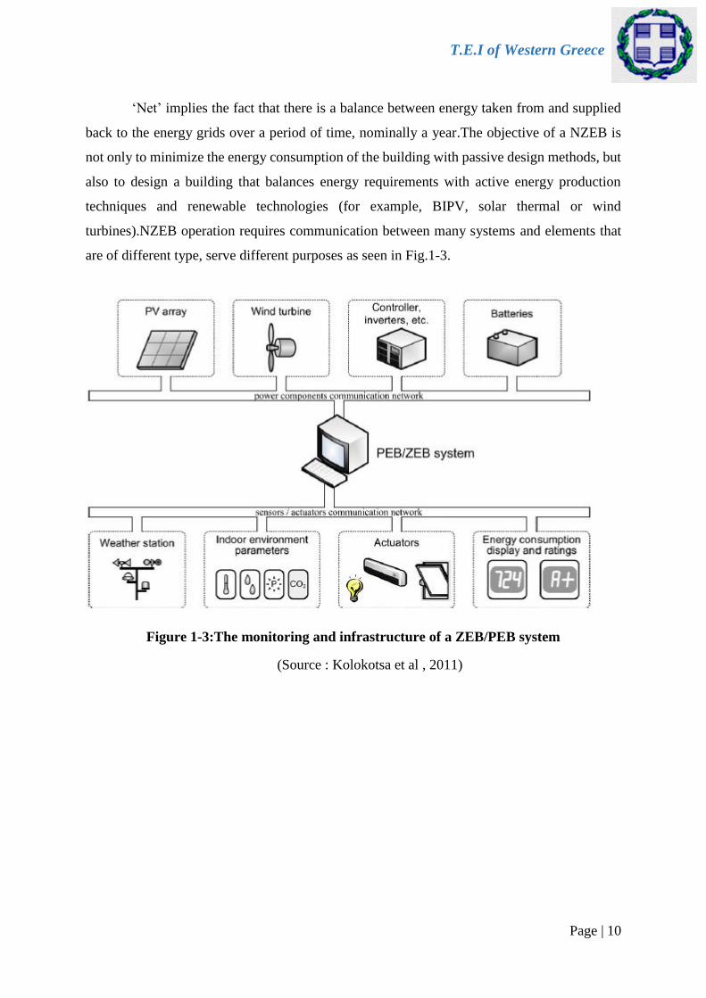
‘Net’ implies the fact that there is a balance between energy taken from and supplied
back to the energy grids over a period of time, nominally a year.The objective of a NZEB is
not only to minimize the energy consumption of the building with passive design methods, but
also to design a building that balances energy requirements with active energy production
techniques and renewable technologies (for example, BIPV, solar thermal or wind
turbines).NZEB operation requires communication between many systems and elements that
are of different type, serve different purposes as seen in Fig.1-3.
Figure 1-3:The monitoring and infrastructure of a ZEB/PEB system
(Source : Kolokotsa et al , 2011)

T.E.I of Western Greece
Page | 11
LITERATURE REVIEW ON ZEB
The study of existing literature revealed that the lack of a commonly agreed ZEB
definition is already widely discussed on the international level(IEA SHC Task 40/ECBCS).
Marszal et al.(2013) in their paper have given an overview of existing ZEB definitions by
highlighting the most important aspects which should be discussed before developing new ZEB
definitions. In addition,they have also presented various approaches towards possible ZEB
calculation methodologies. Their study indicated that the metric of the balance, the period and
the types of energy included in the energy balance together with the renewable energy supply
options, the connection to the energy infrastructure and energy efficiency, the indoor climate
and the building–grid interaction requirements are the most important issues.
The definitions of ZEB require the use of a defined site boundary. The site boundary
represents a meaningful boundary that is functionally part of the building(s). The site boundary
for a Zero Energy Building (ZEB) could be around the building footprint if the on-site
renewable energy is located within the building footprint, or around the building site if some
of the on-site renewable energy is on-site but not within the building footprint. Delivered
energy and exported energy are measured at the site boundary(US DOE).Here,the term
delivered energy signifies the energy delivered to the building from the grid and the exported
energy refers to the excess energy generated by the renewables which is supplied to the grid .

T.E.I of Western Greece
Page | 12
Figure 2-1: Site Boundary of Energy Transfer for Zero Energy Accounting
(Source :U.S. DOE 2015)
Danny et al.(2013) in “Zero energy buildings and sustainable development
Implications” have categorized energy-efficient measures that have significant influence on
energy consumption in buildings into 3 groups .
Building envelopes - thermal insulation, thermal mass, windows/ glazing (including
daylighting) and reflective/green roofs.
Internal conditions - indoor design conditions and internal heat loads (due to electric
lighting and equipment/appliances).
Building services systems - HVAC (heating, ventilation and air conditioning), electrical
services (including lighting) and vertical transportation (lifts and escalators).
In their work, they have also stated that the commonly used options to satisfy the
energy demand in ZEBs by the use of onsite renewables (the first four are usually on-site and
the last option is off-site) are :
PV (Photovoltaic) and BIPV (building-integrated photovoltaic)
Wind turbines

T.E.I of Western Greece
Page | 13
Solar thermal (solar water heaters)
Heat pumps
District heating and cooling.
Figure 2-2:Overview of possible renewable supply options
(Source : Marszal et al.2011)
Fig.2-2 shows the different options available for accessing renewable energy and to
satisfy the energy demand of the building throughout the year.
Kolokotsa et al.(2013) in their work have noted that “Buildings are complex systems
and detailed simulation is needed to take into account the actual climate data, geometries,
building physics, HVAC-systems, energy-generation systems, natural ventilation, user
behaviour (occupancy, internal gains, manual shading), etc. towards a zero or positive energy
approach”. In order to obtain an accurate simulation model, detailed representation of the
building structure and the subsystems is required, but it is the integration of all the systems that
requires significant effort.

T.E.I of Western Greece
Page | 14
Figure 2-3:The components of a ZEB/PEB architecture during real-time operation
(Source :Kolokotsa et al.2013)
Fig.2-3 depicts the PEB/NZEB modeling, building automation components (i.e.
infrastructure and networking) realtime optimization and control of PEB/NZEB operations and
user-interaction .
Lund et al.(2010) examine the role of district Heating in future renewable energy
systems in Denmark. Their study comprised about 25 per cent of the Danish building stock,
which have individual gas or oil boilers and could be substituted by district heating or a more
efficient individual heat source .They concluded that in such a perspective, the best option will
be to combine a gradual expansion of district heating with individual heat pumps in the
remaining buildings.
Wang et al.(2009) have made a case study of Zero Energy building design and
discussed possible solutions for zero energy building design in UK.They summarized the entire
design process into 3 major steps.First,an analysis of the prevailing local climatic conditions is
essential to promote Zero Energy homes. Secondly, the application of passive design methods
and advanced facade designs is required to minimize the load requirement from heating and

T.E.I of Western Greece
Page | 15
Figure 2-4 :Scheme of grid-connected renewable electricity system
(Source : Wang et al .2009)
cooling through building energy simulations. Finally, through the use of simulation software
TRNSYS to investigate various energy efficient mechanical systems and renewable energy
systems including photovoltaic, wind turbines and solar hot water system to enable system
design optimizations.
Systems designed to supply a renewable source of electricity are indispensable in the
delivery of zero energy building designs (Wang et al.2009) . The scheme of a grid connected
renewable electricity system is shown in Fig. 2-4. It is comprised of PV, small wind turbines,
inverters for PV and wind turbine (from AC to DC), a distribution board, meters for export and
import connected to the grid, and electricity loads .
A ZEB can be off-grid or on-grid. The main difference between those two approaches
is that the off-grid ZEB is not connected to the utility grid, and thus it does not purchase energy
from the external sources (Voss et al.2007). In other words, the building offset all required
energy by producing energy from RES. The on-grid ZEB is also an energy producing building,
but with the possibility of both purchasing energy from the grid and feeding excess energy
production back to the grid to return as much energy to the utility as it uses on an annual basis
(Torcellini et al.2006).
T.E.I of Western Greece
Page | 16
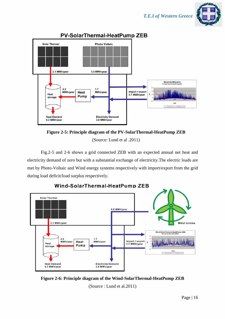
Figure 2-5: Principle diagram of the PV-SolarThermal-HeatPump ZEB
(Source: Lund et al .2011)
Figure 2-6: Principle diagram of the Wind-SolarThermal-HeatPump ZEB
(Source : Lund et al.2011)
Fig.2-5 and 2-6 shows a grid connected ZEB with an expected annual net heat and
electricity demand of zero but with a substantial exchange of electricity.The electric loads are
met by Photo-Voltaic and Wind energy systems respectively with import/export from the grid
during load deficit/load surplus respectively.

T.E.I of Western Greece
Page | 17
Following the earlier paragraph,mismatches may occur from hourly differences in
energy production and consumption at the building level. From the viewpoint of an overall
electricity system,a mismatch can be positive or negative. Lund et al.(2011) in their work have
argued the need to compensate the mismatch of a building by increasing (or decreasing) the
capacity of the energy production unit . In order to quantify the mismatch, they defined four
types of Zero energy buildings .
i) PV ZEB: Building with a relatively small electricity demand and a photovoltaic installation.
ii)Wind ZEB: Building with a relatively small electricity demand and a small on-site wind
turbine.
iii) PV-SolarThermal-HeatPump ZEB: Building with a relatively small heat and electricity
demand and a photovoltaic installation in combination with a solar thermal collector, a heat
pump and heat storage.
iv)Wind-SolarThermal-HeatPump ZEB: Building with a relatively small heat and electricity
demand and a wind turbine in combination with a solar thermal collector, a heat pump and heat
storage.
Their study concluded that mismatch compensation factors are a little below one for buildings
with photovoltaics (PV) and a little above one for buildings with wind turbines

T.E.I of Western Greece
Page | 18
Figure 3-1: Map of India showing Climatic Zones(Based upon survey of India
outline map printed in 1993)
(Source: National Building Code 2005)
METEOROLOGICAL PARAMETERS – DATA
3.1 Climatic Conditions (India)
This Chapter presents the profiles of the Global Solar Radiation,hourly ambient
Temperature that have an impact on the design of a ZEB.The climatic classification map of
India is shown in Fig.3-1. Each climatic zone does not have same climate for the whole year.
A climatic zone that does not have any season for more than six months may be called as
composite zone.The nation has four seasons: winter (January and February), summer (March
to May), a monsoon(rainy) season (June–September), and a post-monsoon period (October–
December).The nation's climate is strongly influenced by the Himalayas and the Thar Desert
[Chang,1967].

T.E.I of Western Greece
Page | 19
Table 3-1 : Classification of Climatic Zones
Figure 3-2: Horizontal Irradiation(average daily)for Chennai
(Source :PVGIS)
For the purpose of design of buildings, the country may be divided into major climatic
zones as given in Table 3-1.
(Source: National Building Code 2005)
3.1.1 Solar Radiation and Temperature Profiles (Chennai)
Fig.3-2 depicts the average daily solar radiation profile on the horizontal for Chennai.

T.E.I of Western Greece
Page | 20
As observed from Fig.3-2,the city receives the maximum and the minimum average
daily Solar Radiation Intensity on the Horizontal in March(7.0kWh/m2/day)and
November(4.5 kWh/m2/day) respectively.
.
Figure 3-3:Hourly Ambient Temperature,Ta profiles on the Representative days of
Seasonal months,Chennai
From Fig. 3-3,it can be inferred that the temperature around solar noon on the
representative days is considerably higher than the temperatures at other hours .For the case of
London and Patras temperature profiles are comparatively smoother as can be observed from
Figs.3-5 & 3-9 respectively.
3.2 Climatic Conditions in England
England is situated to the west of Eurasia and has an extensive coastline. Such a
positioning is responsible for its fairly complex climate, which demonstrates the meeting of the
dry continental air and the moist maritime air. This creates rather large differences in
temperature ranges and also leads to the occurrence of several seasons over the course of one
day. The parts of England closest to the Atlantic Ocean experience the mildest temperatures,
although these are also the wettest and experience the most wind. The areas in the east, on the
other hand, are drier and less windy, but also display cooler temperatures. England is warmer
17.5
20
22.5
25
27.5
30
32.5
35
37.5
40
1 2 3 4 5 6 7 8 9 10 11 12 13 14 15 16 17 18 19 20 21 22 23 24
Tem
per
atu
re(o
C)
Hour
Temperature Profiles
Jan Apr Jul Oct

T.E.I of Western Greece
Page | 21
and sunnier than any of the other countries making up the United Kingdom. The month with
the most sunshine is July, which is also England’s driest month.
3.2.1 Solar Radiation and Temperature Profiles (London)
The figures in this section depict the average daily solar radiation and hourly ambient
temperature profiles of London which is located at geographical co-ordinates of 51.5o N and
0.127oW.
Figure 3-4:Horizontal Irradiation(average daily)for London
(Source :PVGIS)
From Fig.3-4,it can be noticed that London receives maximum and the minimum
average daily Solar Radiation Intensity on the Horizontal in June (5.5 kWh/m2/day)and in
December(0.64 kWh/m2/day) respectively.

T.E.I of Western Greece
Page | 22
0
2.5
5
7.5
10
12.5
15
17.5
20
22.5
25
1 2 3 4 5 6 7 8 9 10 11 12 13 14 15 16 17 18 19 20 21 22 23 24
Tem
per
atu
re (
oC
)
Hour
Temperature Profiles
Jan Apr Jul Oct
Figure 3-5:Hourly Ambient Temperature,Ta profiles on the Representative days of
Seasonal months,London
3.3 Climatic Conditions in Greece
The climate of Greece is predominantly mediterranean with summers that are usually
hot and dry, and the winters that can be quiet cold and wet. The upper part of Greece can be
very cold during the winter. However, for the south of Greece and the islands, the winters will
be milder.Figures 3-6 & 3-7 show the different climatic zones of Greece.

T.E.I of Western Greece
Page | 23
Figure 3-7:Climatic zones according to the new
energy performance regulation(KENAK)[13]
Figure 3-6:Climatic zones according to the
existing thermal insulation regulation of
1979[13]
Figure 3-8:Horizontal Irradiation(average daily)for Patras
(Source : PVGIS)
3.3.1 Solar Radiation and Temperature Profiles
Figures in this section depict the average daily solar radiation and hourly ambient
temperature profiles for Patras located at geographical co-ordinates of 38.25oN and 21.73 oE.

T.E.I of Western Greece
Page | 24
5
7.5
10
12.5
15
17.5
20
22.5
25
27.5
30
32.5
35
1 2 3 4 5 6 7 8 9 10 11 12 13 14 15 16 17 18 19 20 21 22 23 24
Tem
per
atu
re(o
C)
Hour
Temperature Profiles
Jan Apr Jul Oct
Figure 3-9: Hourly Ambient Temperature,Ta profiles on the Representative
days of Seasonal months,Patras
From Fig.3-8 , June and December receive the maximum and the minimum average
daily Solar Radiation Intensity on the Horizontal (8.0 kWh/m2/day)and (1.9 kWh/m2/day)
respectively.
There will be discussion in chapter 5 on how the hourly solar radiation intensity values
and the hourly temperature values influence the calculation of the Solar gain into the building
through the windows and the Space Heating Load of a building respectively.

T.E.I of Western Greece
Page | 25
BUILDING ARCHITECTURE
Optimum level of building insulation not only helps lower monthly energy bills, but
also adds to the overall comfort. Insulation helps maintain comfort temperature by reducing
leakages. With the advent of green technologies and practices, the potential to save energy by
design today can be as high as 40-50 %. Insulation in buildings is assuming tremendous
importance and has a potential to reduce energy consumption .Buildings without insulation and
air-tight envelope can result in major energy wastage[Building Insulation Bulletin –Indian
Green Building Council,April 2008].
Benefits of Insulation
Provides thermal as well as acoustical insulation.
Resistant to moisture.
Resistant to air infiltration.
Applications of Insulation materials
Exterior walls.
Interior walls
Over the deck (roof)
4.1 Properties to consider in the selection of Insulation materials
R-value: Insulation is rated in terms of thermal resistance, called R-value, which indicates the
resistance to heat flow. The higher the R-value, the greater the insulating effectiveness. The R-
value of thermal insulation depends on the type of material, its thickness and its density. R-
value is the reciprocal of the time rate of heat flow through a unit area induced by a unit
temperature difference between two defined surfaces of material or construction under steady-
state conditions. R-value is expressed in m² K/W
U-factor (thermal transmittance) : The heat transmission in unit time through unit area of a
material or construction and the boundary air films, induced by unit temperature difference
between the environments 2 on each side. U-value is expressed in W/m2K. The relationship
between U-factor and R-value is not always exactly the inverse and therefore R-value cannot

T.E.I of Western Greece
Page | 26
Table 4-1: Maximum U Values(W/m2K)
Source : The Building Regulations 2000 (England and Wales)
Table 4-2:The elemental U-value(W/m2K) requirements for new build under
four EU country’s Regulations (EST, 2002)
be precisely extrapolated for a material of different thickness. However, assuming an inverse
relationship may be adequate
Fabric Heat Loss : Building regulations deal with design standards for fabric heat loss, and
have historically set minimum insulation levels in terms of elemental U values. Each element
of the building envelope (roof, wall, floor, window, door) is assigned a maximum heat loss
rate. The unit of measurement, Watts per square metre Kelvin (W/m2K), is an expression of
how quickly energy passes through a square metre of the element for a given temperature drop
between inside and out. The aim is to slow down the rate of heat loss, which means a lower U
value.
4.2 Building Regulations and the EU
Table 4-2 compares Building Regulations in England and Wales, Denmark and The
Netherlands. These countries are chosen because of the broad similarities in climate. Data on
Sweden is included as it is presently the best EU standard. The standards required in Denmark
are much higher than England and Wales and were also issued over 4 years before. As a result
of these regulations a detached building built to the latest standards in England and Wales
consumes nearly 20% more energy than an equivalent home in Denmark.

T.E.I of Western Greece
Page | 27
4.2.1 Building Regulation (Greece)
In Greece, the regulation of energy efficient buildings KENAK refers to the standard
ISO 13790 as well as other international standards that define all the parameters related to the
Greek requirements. Since the implementation of Energy Performance of Buildings
Directive(EPBD), there were not any specific regulations defined in Greece regarding the
energy performance and the evaluation of buildings. The only regulations related with the
thermal performance of building were the national Thermal Insulation Regulation (TIR)
introduced in 1981 and the Technical codes related with the installation of heating and cooling
systems[22]. The thermal insulation regulations required to achieve low U values are given
below. The smaller the U value is, less thermal loss exists and the better the insulation of the
building is. The U value had to be lower than the value that the regulations indicated.
Table 4-3:Minimum U values(W/m2K) according to the new and previous regulations[23]
4.2.2 Building Regulation(India)
Table 4-4 shows the Building envelope requirements for Non-residential and Residential
as per ASHRAE.

T.E.I of Western Greece
Page | 28
Table 4-6:Opaque Wall assembly U-factor and Insulation R-value Requirements
Table 4-5:Roof assembly U-factor and Insulation R-value Requirements
Table 4-4:ASHRAE* Building Envelope Requirements
(Source :Building Insulation,Indian Green Building Council)
Tables 4-5 and 4-6 show the U-factor and Insulation R-value requirements for each
climatic zones in India.
(Source :Energy Conservation Building Code,2006)
(Source :Energy Conservation Building Code,2006)

T.E.I of Western Greece
Page | 29
CALCULATION OF BUILDING LOADS(THERMAL
AND ELECTRIC)
5.1 Determination of Thermal Heat losses Coefficient (UA)b of a
Building
The following example outlines the process for calculating the Heat Losses coefficient
,U of the Building (Douglas J.Harris,2015).The U-value is a measure of the heat transfer
through a building element such as a wall and is measured in W/m2K. It can be considered to
comprise three main thermal resistances: the inner surface resistance,the resistance to
conduction of the wall itself, and the outer surface resistance. The wall resistance is the sum of
the resistances of the individual layers; the resistance of each layer is simply the thickness tn
divided by its thermal conductivity kn.
𝑈 =
1
𝑅𝑡 5-1
Rt = Rsi + Rw + Rso
Rw = R1 + R2 + …
𝑅𝑛 =
𝑡𝑛
𝑘𝑛 5-2
For a single-leaf brick wall in a ‘normal’ location (neither highly sheltered nor highly exposed)
the following values are used:
Without insulation :
tw = 105 mm, kw = 0.44
Rw = 0.105/0.44 = 0.238 m2K/W
Rsi = 0.123 m2K/W
Rso = 0.055 m2K/W
Rt = 0.123 + 0.238 + 0.055
= 0.417 m2K/W
U = 2.4W/m2K.
T.E.I of Western Greece
Page | 30
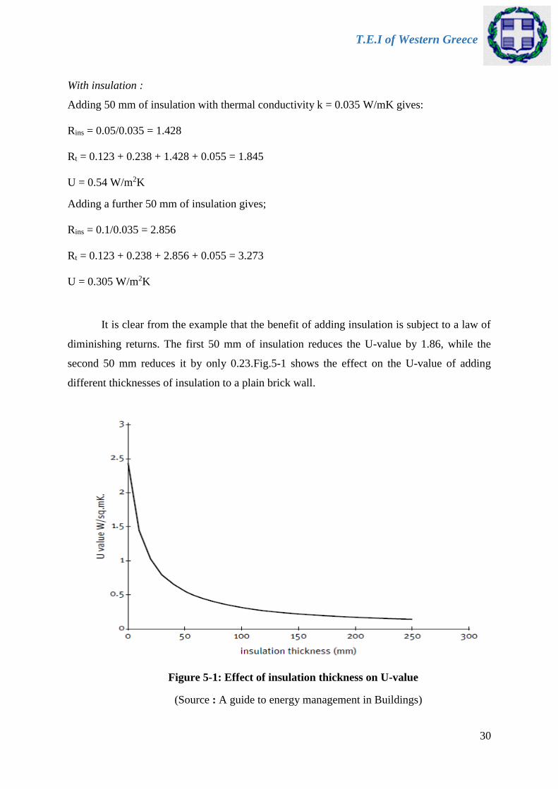
Figure 5-1: Effect of insulation thickness on U-value
With insulation :
Adding 50 mm of insulation with thermal conductivity k = 0.035 W/mK gives:
Rins = 0.05/0.035 = 1.428
Rt = 0.123 + 0.238 + 1.428 + 0.055 = 1.845
U = 0.54 W/m2K
Adding a further 50 mm of insulation gives;
Rins = 0.1/0.035 = 2.856
Rt = 0.123 + 0.238 + 2.856 + 0.055 = 3.273
U = 0.305 W/m2K
It is clear from the example that the benefit of adding insulation is subject to a law of
diminishing returns. The first 50 mm of insulation reduces the U-value by 1.86, while the
second 50 mm reduces it by only 0.23.Fig.5-1 shows the effect on the U-value of adding
different thicknesses of insulation to a plain brick wall.
(Source : A guide to energy management in Buildings)

T.E.I of Western Greece
Page | 31
The Overall U-Value of the building is given by the equation :
𝑈 =
1
𝑅= (
1
ℎ𝑖+ 𝛴
𝛥𝑥
𝑘+
1
ℎ𝑜)
−1
5-3
Where 1/hi and 1/ho represent the thermal resistances inside and outside the building.
ℎ𝑖 = ℎ𝑐,𝑖 + ℎ𝑟,𝑖 5-4
Where hc,i and hr,i are the convective and the radiative components of the resistances
respectively.
The U-Value and the thermal resistance,R of the individual components of the building per unit
area are given by :
1
𝑢𝑤𝑎𝑙𝑙= 𝑅𝑤𝑎𝑙𝑙 =
1
ℎ𝑖𝐴𝑤𝑎𝑙𝑙+ 𝛴 (
𝛥𝑥
𝑘𝐴𝑤𝑎𝑙𝑙) +
1
ℎ𝑜𝐴𝑤𝑎𝑙𝑙 5-5
1
𝑢𝑤𝑖𝑛𝑑𝑜𝑤𝑠= 𝑅𝑤𝑖𝑛𝑑𝑜𝑤𝑠 =
1
ℎ𝑖𝐴𝑤𝑖𝑛𝑑𝑜𝑤𝑠+ 𝛴 (
𝛥𝑥
𝑘𝐴𝑤𝑖𝑛𝑑𝑜𝑤𝑠) +
1
ℎ𝑜𝐴𝑤𝑖𝑛𝑑𝑜𝑤𝑠 5-6
1
𝑢𝑑𝑜𝑜𝑟= 𝑅𝑑𝑜𝑜𝑟 =
1
ℎ𝑖𝐴𝑑𝑜𝑜𝑟+ 𝛴 (
𝛥𝑥
𝑘𝐴𝑑𝑜𝑜𝑟) +
1
ℎ𝑜𝐴𝑑𝑜𝑜𝑟 5-7
Therefore,
(𝑈𝐴)𝑏 = 𝛴 (1
ℎ𝑖+ 𝛴
𝛥𝑥
𝑘+
1
ℎ𝑜)
−1
𝐴 5-8
For the sake of calculation,in all the cities,hc,i =5 W/m2K ,hr,i = 5Wm2K and ho =
20W/m2K (for London),ho = 15W/m2K (for Patras) and ho = 10 W/m2K(for Chennai).The value
of ho which is dependent on the wind speed is choosen based on the wind speed in each city .

T.E.I of Western Greece
Page | 32
5.1.1 Calculation of (UA)b of the Building
A single storey building is considered in all 3 cities with the dimensions and building
elements as given in Tables 5-1 & 5-2.
Table 5-1: Building Parameters
Parameter Value
Length 15m
Width 10m
Height 3m
Roof Plaster-Wood-Insulation -Roof Tile
Roof Inclination(London) 40o
Roof Inclination(Patras) 10o
Terrace Elements(Chennai) Plaster – Brick – Concrete - Tiles
Note : For the same building in Chennai ,there is no roof but only terrace
Table 5-2:Building Elements
Façade
Facing Elements
South
2 Vertical sealed double glazed window with distance between glasses
20mm (2m X 1.5m) ,Wooden door (25mm thickness,1m length and 1.5m
Height,Wall comprising the layer : Plaster-Brick-Insulation-Brick-Plaster
North
2 Vertical sealed double glazed window with distance between glasses
20mm (2m X 1.5m), Wall comprising the layer : Plaster-Brick-Insulation-
Brick-Plaster
West
1 Vertical sealed double glazed window with distance between glasses
20mm (2m X 1.5m), Wall comprising the layer : Plaster-Brick-Insulation-
Brick-Plaster
East
1 Vertical sealed double glazed window with distance between glasses
20mm (2m X 1.5m),Wall comprising the layer : Plaster-Brick-Insulation-
Brick-Plaster
Table 5-3: Building Elements Thickness and Thermal Conductivity
(Source :ASHRAE)
Building
Element Element Layers
Thickness,t
(m)
Thermal
Conductivity,k
(W/m.k)
Thermal
Resistance,R(m2K/
W)= t/k
Roof
Plaster Board 0.013 0.581 0.022
Wood 0.020 0.465 0.043
Polystyrene
(London/Patras/
Chennai)
0.067,0.066,0.076 0.034 1.976,1.947,2.235
Roof Tile 0.030 0.233 0.129
Total resistance of roof(conduction part) 2.547

T.E.I of Western Greece
Page | 33
hi(W/m2K) 10
ho(W
/m2K)
20
Facade
Facing
Length,m 2 1 2 2 2 15
Height,m 1.5 1.5 1.5 1.5 1.5 13.054
Area,m2 6 1.5 37.5 6 39 6 24 6 24 195.811
Thermal
Resistance,
R(m2K/W)
0.081 0.238 0.074 0.081 0.071 0.081 0.116 0.081 0.116 0.012
RoofWindow
(1 no.)Description
Window
(2 no.s)
Door
(1
no.)
South North West East
WallWindow
(2 no.s)Wall Wall Wall
Window
(1 no.)
Total Resistance of the building,Rb (m2K/W) 0.948
U-Value of the Building(1/Rb),(W/m2K) 1.055
(UA)b of the building (W/K) 364.765
Wall
Plaster 0.020 0.727 0.028
Brick 0.100 1.333 0.075
Insulation
(London/Patras/
Chennai)
0.104,0.075,0.055 0.043 2.419,1.744,1.279
Brick 0.100 1.333 0.075
Plaster 0.020 0.727 0.028
Total resistance of Wall(conduction part) 1.019
Door Wood 0.025 0.121 0.207
Terrace
Plaster 0.013 0.581 0.022
Brick 0.1 1.333 0.075
Concrete 0.1 0.813 0.123
Tile 0.030 0.233 0.129
Total resistance of Terrace(conduction part) 0.349
As observed in Table 5-3,only the thickness of polystyrene in the Roof and the thickness
of insulation in the wall changes between the three cities.The thermal Resistance, R pertaining
to the conduction part(Δx/k) is calculated for each of the components of the building in Table
5-3 .
Table 5-4:(UA)b of the building (London)
In Table 5-4,the wall area is calculated by subtracting the area of the windows (and
door for south façade)from the total area of each façade .The total area of the facades facing
North and South are (15mX3m) = 45 m2 and the total area of the facades facing East and west
are (10mX3m) = 30m2.The thermal resistance,R of each component of the building on all
facades is determined by equations (5-5) to (5-7).Τhe total thermal resistance of the building is

T.E.I of Western Greece
Page | 34
hi(W/m2K) 10
ho(W
/m2K)
15
Facade
Facing
Length,m 2 1 2 2 2 15
Height,m 1.5 1.5 1.5 1.5 1.5 10.154
Area,m2 6 1.5 37.5 6 39 6 24 6 24 152.314
Thermal
Resistance,
R(m2K/W)
0.083 0.249 0.056 0.083 0.054 0.083 0.088 0.083 0.088 0.015
Wall
South North West East
RoofWindow
(1 no.)Wall
Window
(1 no.)WallDescription
Window
(2 no.s)
Door
(1
no.)
WallWindow
(2 no.s)
U-Value of the Building(1/Rb),(W/m2K) 1.131
(UA)b of the building (W/K) 341.852
Total Resistance of the building,Rb (m2K/W) 0.884
the sum of all individual resistance of all components on all facades. The U-Value of the
building is then the reciprocal of R as given by equation (5-3).Finally,the total Heat Loss
coefficient of the building, (UA)b is calculated by multiplying the U-value of the building with
the total surface area of the building as in equation (5-8).
The above calculation procedure is repeated for the building in Patras,Greece by
changing the Roof inclination to 10o and the (UA)b is calculated as shown in Table 5-5 .
Table 5-5: (UA)b of the building(Patras)
For the building in Chennai,the only change from that of the buildings in London and
Patras is that the roof is replaced by a terrace with the procedure for calculating (UA)b
remaining the same .The (UA)b for the building in Chennai is shown in Table 5-6.

T.E.I of Western Greece
Page | 35
Table 5-7: Heating and Cooling Degree Days(Chennai)
(Source :RetScreen)
Table 5-6:(UA)b of the building (Chennai)
5.2 Heating and Cooling Degree Days for 3 cities
From Table 5-7,it can be noticed that the average ambient temperatures in all the
months is greater than the reference temperature selected to exist in the building
i.e.,22oC.Hence the building in Chennai will have Cooling Loads prominently and no Heating
Loads .
Table 5-7 is presented here to suggest that further in the chapter,only the cooling loads
of the the building in Chennai will be calculated as there are no Heating Loads .
hi(W/m2K) 10
ho(W
/m2K)
10
Facade
Facing
Length,m 2 1 2 2 2 15
Height,m 1.5 1.5 1.5 1.5 1.5 10.000
Area,m2 6 1.5 37.5 6 39 6 24 6 24 150.000
Thermal
Resistance,
R(m2K/W)
0.089 0.271 0.045 0.089 0.043 0.089 0.070 0.089 0.070 0.018
Wall
South North West East
TerraceWindow
(1 no.)Wall
Window
(1 no.)WallDescription
Window
(2 no.s)
Door
(1
no.)
WallWindow
(2 no.s)
U-Value of the Building(1/Rb),(W/m2K) 1.146
(UA)b of the building (W/K) 343.802
Total Resistance of the building,Rb (m2K/W) 0.873

T.E.I of Western Greece
Page | 36
Table 5-8: Heating /Cooling Degree Days London
(Source :RETSCREEN)
Tables 5-8 and 5-9 present the Heating and Cooling Degree days for London and
Paptras respectively .It can be seen that the annual Heating Degree-days and the annual Cooling
Degree-days for the building located in London is 2,370oC-d and 1,043 oC-d respectively.
Table 5-9:Heating /Cooling Degree Days Patras
(Source :RETSCREEN)

T.E.I of Western Greece
Page | 37
Representative
Day,nTanφ Tanδ
Degrees Radians Degrees Radians Degrees Radians
51.51 0.90 0.13 0.00 17 -20.92 -0.37
Region -London
Located in : UK
Month Considered for the Analysis : January
1.26 -0.38
Latitude,φ Longitude Declination Angle,δ
The annual Heating Degree-days and the annual Cooling Degree-days for the building
located in Patras is 1,076oC-d and 2,742oC-d respectively.However,it is to be noted that the
above Tables have shown the Heating Degree days calculated for a base temperature of 18oC
and the cooling Degree days for a base temperature of 10oC whereas the reference temperature
selected inside the building is 22oC.Hence,while calculating the thermal loads(Heating and
Cooling) the degree days from the above tables are converted to the reference temperature of
22oC by means of suitable equations which will be enlisted further in this chapter.
5.3 Calculation of Solar Gain for the Windows in
London,January
Before introducing the concept of renewables inside the building to satisfy the Load
demand,it is of utmost importance to minimize the energy demand inside the building by means
of passive solar techniques and factoring the solar gain inside the building which will reduce
the building Heating Loads .From Table I-B in Appendix I, the global solar radiation intensity
for each hour is calculated and tabulated as follows :
Table 5-10: Solar Radiation Intensity, London on representative day for January
Time Interval
Hourly Global Solar
Radiation Intensity on
the horizontal(W/m2)
8:00AM-9:00AM 35.75
9:00AM-10:00AM 85.75
10:00AM-11:00AM 119.5
11:00AM-12:00PM 137
12:00PM-1:00PM 137
1:00PM-2:00PM 119.5
2:00PM-3:00PM 85.75
3:00PM-4:00PM 42
The declination angle δ is calculated by means of the following equation :
δ = 23.45 ∗ Sin (360 ∗284 + n
365) 5-9

T.E.I of Western Greece
Page | 38
The Hourly Clearness index value KT is calculated by :
𝐾𝑇 =𝐼
𝐼𝑒𝑥𝑡
5-10
Where I is the hourly Global Solar Radiation Intensity,Iext is the intensity of the solar radiation
which reaches the outer space of the earth’s atmosphere given by
𝐼𝑒𝑥𝑡 = (12 ∗3600
𝜋) . 𝐺𝑠𝑐(1 + 0.033
∗ 𝐶𝑜𝑠(360𝑛
365)[(𝐶𝑜𝑠(𝜑). 𝐶𝑜𝑠(𝛿). (𝑆𝑖𝑛𝜔2 − 𝑆𝑖𝑛𝜔1))
+ 2𝜋(𝜔2 − 𝜔1). 𝑆𝑖𝑛(𝜑).𝑆𝑖𝑛(𝛿)
360)
5-11
Isc is the solar constant and is equal to 1353 W/m2
ω is the hour angle
The fraction of diffuse based on the value of KT is taken from Table 5-11 .
Table 5-11:Fraction of Diffuse given by Orgill and Hollands Model
Fraction of
Diffuse Value Range
Id/I
1.0-0.249KT KT <0.35
1.557-1.84KT 0.35<KT<0.75
0.177 KT >0.75
The Hourly Beam radiation is determined by the following equation.
𝐼𝑏 = 𝐼 − 𝐼𝑑 5-12
Where ,
Ib is the Beam Radiation intensity in W/m2
I is the Global Solar Radiation intensity in W/m2
Id is the Diffuse Radiation intensity in W/m2

T.E.I of Western Greece
Page | 39
8:00AM-9:00AM -60 -45 35.75 266.20 0.134 0.967 34.55 1.20
9:00AM-10:00AM -45 -30 85.75 415.77 0.206 0.949 81.35 4.40
10:00AM-11:00AM -30 -15 119.5 521.53 0.229 0.943 112.68 6.82
11:00AM-12:00PM -15 0 137 576.28 0.238 0.941 128.89 8.11
12:00PM-1:00PM 0 15 137 576.28 0.238 0.941 128.89 8.11
1:00PM-2:00PM 15 30 119.5 521.53 0.229 0.943 112.68 6.82
2:00PM-3:00PM 30 45 85.75 415.77 0.206 0.949 81.35 4.40
3:00PM-4:00PM 45 60 42 266.20 0.158 0.961 40.35 1.65
Total 762.25
Hourly
Diffuse
Radiation
(W/m2),Id
Hourly
Beam
Radiation(
W/m2),Ib
Percentage(%)
of Diffuse(Id/I)
Intensity of Extra-
Terrestrial
Radiation,Iext
Hourly
Clearness
Index,KT
Time Interval ω1 ω2
Hourly Solar
Radiation
Intensity,Ih(W/
m2)on the
representative
day(n=17)
Table 5-12: Hourly Beam and Diffuse Radiation
The different parameters calculated by using the equations (5-10) to (5-12) are tabulated in
Table 5-12 :
For obtaining the value of Transmittance τ, the glass window is assumed to have the
following properties :
Table 5-13: Properties of Glass Windows
Thickness of Glass,L = 0.003m
Extinction Coefficient of Glass, λ = 10m-1
Angle of incidence of the Solar Beam Angle of
Refraction,θ1 = 30o
Refractive Index of the Glass = 1.52
Angle of Refraction,θ2 is determined using Snell’s law which is given by :
Sin(θ1)/Sin(θ2) = n 5-13
The coefficient of transmission τα is given by:

T.E.I of Western Greece
Page | 40
Angle of incidence
of solar
Beam,θ1(degrees)
Refractive
Index of
Glass
Angle of
Refraction,θ2
(degrees)
Coefficient of
Transmission,τα
rn rp
Transmission
Coefficient ,τr
Transmission
Co-
efficient,τ=τα*τr
30 1.52 19.2049 0.9687 0.0612 0.0271 0.9160 0.8873
Table 5-14: Transmission Coefficient of Glass
𝛕𝛂 = exp((−λL/Cos(θ2)) 5-14
The reflection coefficients for the two polarized components at the normal and parallel plane
to the medium in which the beam travels is given by :
𝑟𝑛 = 𝑆𝑖𝑛2(𝜃2 − 𝜃1)/𝑆𝑖𝑛2(𝜃2 + 𝜃1) 5-15
𝑟𝑝 = 𝑡𝑎𝑛2(𝜃2 − 𝜃1)/𝑡𝑎𝑛2(𝜃2 + 𝜃1) 5-16
The transmission coefficient τr of the medium is given by :
𝜏𝑟 =
1
2∗ [
1 − 𝑟𝑝
1 + 𝑟𝑝+
1 − 𝑟𝑛
1 + 𝑟𝑛] 5-17
The transmission coefficient of the Glass is given by :
𝜏 = 𝜏𝛼 . 𝜏𝑟 5-18
The above terms are calculated and tabulated as below :
The transmission coefficient of the Glass Windows is therefore 0.88 and the hourly Solar Gain
is calculated as shown in Table 5-15 .
T.E.I of Western Greece
Page | 41
Degrees Radians Degrees Radians
90 1.571 0 0.000 Absorptance,α 1
Time IntervalHour
Angle,ωCOSθ COSθZ
Rb
=(COSθ)/(COS
θZ)
Hourly
Solar
Radiation
Intensity on
the
Windows(
W/m2),IT
Hourly Solar
Gain(W/m2),ITτα
8:00AM-9:00AM -45 0.739 0.132 5.613 23.99 21.11
9:00AM-10:00AM -30 0.855 0.224 3.817 57.48 50.59
10:00AM-11:00AM -15 0.928 0.282 3.290 78.77 69.32
11:00AM-12:00PM 0 0.953 0.302 3.157 90.05 79.24
12:00PM-1:00PM 15 0.928 0.282 3.290 91.13 80.19
1:00PM-2:00PM 30 0.855 0.224 3.817 82.37 72.48
2:00PM-3:00PM 45 0.739 0.132 5.613 65.39 57.55
3:00PM-4:00PM 60 0.588 0.011 52.159 106.24 93.49
Total 595.42 523.97
Τransmission
Coefficient,τ of
Glass Windows
0.88
Angle of orientation,γAngle of inclination ,β
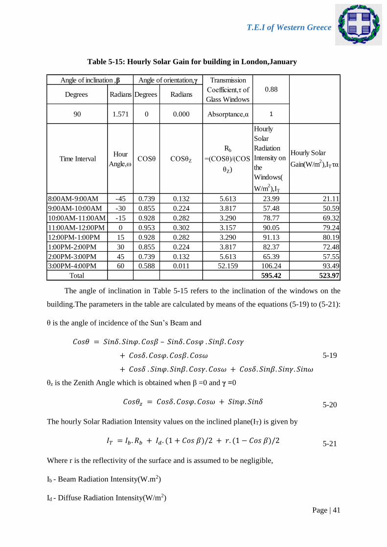
Table 5-15: Hourly Solar Gain for building in London,January
The angle of inclination in Table 5-15 refers to the inclination of the windows on the
building.The parameters in the table are calculated by means of the equations (5-19) to (5-21):
θ is the angle of incidence of the Sun’s Beam and
𝐶𝑜𝑠𝜃 = 𝑆𝑖𝑛𝛿. 𝑆𝑖𝑛𝜑. 𝐶𝑜𝑠𝛽 – 𝑆𝑖𝑛𝛿. 𝐶𝑜𝑠𝜑 . 𝑆𝑖𝑛𝛽. 𝐶𝑜𝑠𝛾
+ 𝐶𝑜𝑠𝛿. 𝐶𝑜𝑠𝜑. 𝐶𝑜𝑠𝛽. 𝐶𝑜𝑠𝜔
+ 𝐶𝑜𝑠𝛿 . 𝑆𝑖𝑛𝜑. 𝑆𝑖𝑛𝛽. 𝐶𝑜𝑠𝛾. 𝐶𝑜𝑠𝜔 + 𝐶𝑜𝑠𝛿. 𝑆𝑖𝑛𝛽. 𝑆𝑖𝑛𝛾. 𝑆𝑖𝑛𝜔
5-19
θz is the Zenith Angle which is obtained when β =0 and γ =0
𝐶𝑜𝑠𝜃𝑧 = 𝐶𝑜𝑠𝛿. 𝐶𝑜𝑠𝜑. 𝐶𝑜𝑠𝜔 + 𝑆𝑖𝑛𝜑. 𝑆𝑖𝑛𝛿 5-20
The hourly Solar Radiation Intensity values on the inclined plane(IT) is given by
𝐼𝑇 = 𝐼𝑏 . 𝑅𝑏 + 𝐼𝑑. (1 + 𝐶𝑜𝑠 𝛽)/2 + 𝑟. (1 − 𝐶𝑜𝑠 𝛽)/2 5-21
Where r is the reflectivity of the surface and is assumed to be negligible,
Ib - Beam Radiation Intensity(W.m2)
Id - Diffuse Radiation Intensity(W/m2)

T.E.I of Western Greece
Page | 42
Table 5-16: Solar gain (daily&monthly)for 3 cities
Jan Apr Jul Oct Jan Apr Jul Oct Jan Apr Jul Oct
day(wh) 523.97 2173.23 1869.89 1172.77 1676.22 2488.49 1704.08 3020.92 3528.11 1132.35 942.23 2143.81
month(kWh) 97.46 391.18 347.80 218.14 311.78 447.93 316.96 561.89 656.23 203.82 175.25 398.75
Chennai
Solar Gain per
London Patras
Rb – Conversion factor of the Beam component from horizontal to Inclined
The total area of the Windows on the South Wall of the Building is (2mX1.5m)*2 = 6 m2
Hence the solar gain into the Building for the entire month of January = 523.97*31*6
= 97,458.42Wh
= 97.46kWh
The process for calculating Solar gain enlisted in this section is repeated for the other
cities for all seasonal months and tabulated as shown in Table 5-16 .
5.4 Calculation of Space Heating, Cooling and other thermal
Loads
In this section,the heating and the cooling Loads of the building are calculated.To
calculate the same,the following are the parameters assumed to exist in the building.
Number of Occupants = 3
Mean Daily Water Consumption per occupant = 50 l
Mean Daily Operation of the hot water returns ,t = 16 h
Length of the Pipes ,l = 30m
Table 5-17: Mains Cold Water Temperature in 3 cities (For Patras taken from TECSOL
and assumed values for other 2 cities)
City Month Temperature(oC)
Patras
Jan 12.8
Apr 14.8
Jul 24.4
Oct 22.3

T.E.I of Western Greece
Page | 43
London
Jan 10.8
Apr 12.8
Jul 22.4
Oct 20.3
Chennai
Jan 17.8
Apr 19.8
Jul 25.4
Oct 23.0
The Load of Space Heating is given by
Lsh = 24 (𝐡
𝐝𝐚𝐲) ∗ (UA)b(𝐖 𝐩𝐞𝐫 𝐂𝐨 ) ∗ D(𝐨𝐂. 𝐝𝐚𝐲) 5-22
D is the degree-days of the sizing month
To convert the degree-days to a reference temperature Tref other than 18oC
D = {N. ΔΤb + (0.744 + 0.00387Dα– 0.5 ∗ 10−6
∗ Dα2 ). N. exp (− [
ΔΤb + 11.11
9.02]
2
)}
5-23
Where
ΔΤb = Tref - Ta
Dα is the annual degree-days at a temperature base of 18oC (which can be obtained from Tables
5-8 & 5-9 for London and Patras respectively).
(UA)b is the product of the overall mean heat transfer coefficient with the area of the external
building surface.
The Load of Water Heating is given by :
Lw = N. Vw. ρ. Cp(Tw − Tm) 5-24
Where
N is the number of days of the month
Vw is the mean daily water consumption/occupant X the number of occupants

T.E.I of Western Greece
Page | 44
Tw is the Desired water temperature
Tm is the mains(Cold)Water Temperature
The Heat Losses in the Pipes is given by:
Lp = N. t. U. l 5-25
Where
t is the mean daily operation of the hot water returns (s)
l is the length of the pipes(m)
U is the mean heat losses coefficient in the pipes(W/m)
Total Load of Water Heating is
Lh,w = Lw + Lp 5-26
5.4.1 Space Heating & other Thermal Loads for London,Patras
To determine the load of space Heating,the Heating Degree days given for a base
temperature of 18oC for cities London and Patras are taken from corresponding Tables 5-8 , 5-
9 and converted to the reference temperature inside the building i.e.,22oC by using equation 5-
23.Following this,the load of space Heating is calculated using equation 5-12 by substituting
the converted Degree Days (D) and the (UA)b values for the respective city.The domestic Hot
water load and the Heat losses in the pipes are calculated by equations (5-24) and (5-25)
respectively. The calculated results are presented in Table 5-18.
Table 5-18: Thermal Loads for the Building in London and Patras
(Reference Temperature inside the building :22oC)
Load London Patras
Jan Apr Jul Oct Jan Apr Jul Oct
Heating
(kWh) 4396.7 3284.9 1045.9 2535.4 3053.6 1837.2 0 858.317
Cooling
(kWh) - - 184.80 - 0 294.68 927.91 94.05
Domestic
Hot
Water(kWh)
265.89 236.40 234.99 214.55 255.08 236.40 192.39 203.74
Heat
Losses(kWh) 307.48 273.37 203.20 248.11 294.98 273.37 222.49 235.61

T.E.I of Western Greece
Page | 45
5.4.2 Space Heating Load calculation (Alternative approach by
using hourly temperature data)
In section 5.4.1 , the space Heating loads were calculated by considering the monthly
average ambient temperature value provided by RetScreen.In this section ,the values of the
hourly temperature for a range of -3 to +3 days around the representative day of the month are
obtained from MeteoNorm database. For each of these 7 days,the difference Ta and Tref(22oC)
(Tref – Ta) is calculated for each hour and added and the average of the 7 days is taken as the
average Degree days for the respective month.This value when multiplied with the number of
days of the month gives the total Heating Degree days for the corresponding month. If Ta is
greater than Tref ,it pertains to a cooling load .
To calculate the Space Heating load in January for London ,the hourly temperature
data for + 3 days representative days is obtained from Meteonorm as shown in Table 5-19.
Table 5-19:Hourly Temperature values + 3 days representative day for London ,
January(n=17)
(Source : Meteonorm)
Hour Ref
Temp(oC)
Hourly Temperature (oC)
14th day 15th day 16th day 17th day 18th day 19th day 20th day
1 22 10.7 12.3 7.2 6.5 6 5.9 1.8
2 22 10.2 11.4 7 7.1 5.7 6.1 1.6
3 22 10.5 10.3 7.8 7.4 5 5.9 2.2
4 22 10.9 9.8 7.3 7.3 4.6 5.5 1.1
5 22 11.1 10.4 6.5 6.7 4.3 4.9 0.6
6 22 10.9 10.3 6.7 7.4 4.1 3.8 0.7
7 22 11.8 10.6 7.2 7.6 3.8 3.8 0.9
8 22 11.7 10.8 7.7 6.9 3.8 4 0.9
9 22 11.4 10.5 7.1 7.3 4.1 3.9 0.4
10 22 11.6 9.8 6.9 7 4.1 3.8 0.5
11 22 11.9 10.6 6.3 6.2 4.5 4.3 0.5
12 22 12.3 10.4 7 6 5.7 4.4 0.9
13 22 12.4 11.1 8 5.8 6.3 4.9 0.9
14 22 12.8 10.5 8 6.3 7.2 5.8 1.7
15 22 12.5 10.1 8.5 6.2 7.4 5.9 2.3
16 22 13.1 10.1 8.1 5.8 7 6 2.6
17 22 12.6 9.9 7.8 5.7 6.9 4.6 1.3
18 22 12.9 9.5 7.6 5.4 6.4 4.5 0.2

T.E.I of Western Greece
Page | 46
19 22 12.7 9.2 7.5 5.9 6.5 4.3 -0.2
20 22 12.8 8.4 7.1 5.3 7 3.3 0.1
21 22 12.1 7.9 6.7 6 6.9 2.7 -0.7
22 22 12.4 8 6.6 6.3 6 2.8 -1.2
23 22 12.1 7.4 6.8 5.8 5.9 2.8 -0.9
24 22 11.9 6.6 6.4 6.3 6.4 2.4 -1.2
For each of these days,the difference between the reference temperature,Tref(oC)and the
ambient temperature,Ta(oC) is calculated for each hour.Adding the 24 values obtained for each
day gives the Heating Degree days(HDD) for the respective day.The average of the Heating
Degree days is taken for the 7 days considered above.This gives the monthly average Heating
Degree days. Multiplying this monthly average HDD value with the number of days in the
month gives the Heating Degree days for the month.Finally,this total degree days for the month
is multiplied with the (UA)b of the building of the respective city to obtain the Load of Space
Heating as shown in Table 5-20.
Table 5-20:Space Heating Load considering hourly values of temperature
London(January)
Hour Tref - Ta(oC)[+ 3 days around representative day]
14th day 15th day 16th day 17th day 18th day 19th day 20th day
1 11.3 9.7 14.8 15.5 16 16.1 20.2
2 11.8 10.6 15 14.9 16.3 15.9 20.4
3 11.5 11.7 14.2 14.6 17 16.1 19.8
4 11.1 12.2 14.7 14.7 17.4 16.5 20.9
5 10.9 11.6 15.5 15.3 17.7 17.1 21.4
6 11.1 11.7 15.3 14.6 17.9 18.2 21.3
7 10.2 11.4 14.8 14.4 18.2 18.2 21.1
8 10.3 11.2 14.3 15.1 18.2 18 21.1
9 10.6 11.5 14.9 14.7 17.9 18.1 21.6
10 10.4 12.2 15.1 15 17.9 18.2 21.5
11 10.1 11.4 15.7 15.8 17.5 17.7 21.5
12 9.7 11.6 15 16 16.3 17.6 21.1
13 9.6 10.9 14 16.2 15.7 17.1 21.1
14 9.2 11.5 14 15.7 14.8 16.2 20.3
15 9.5 11.9 13.5 15.8 14.6 16.1 19.7
16 8.9 11.9 13.9 16.2 15 16 19.4
17 9.4 12.1 14.2 16.3 15.1 17.4 20.7
18 9.1 12.5 14.4 16.6 15.6 17.5 21.8
19 9.3 12.8 14.5 16.1 15.5 17.7 22.2
20 9.2 13.6 14.9 16.7 15 18.7 21.9

T.E.I of Western Greece
Page | 47
21 9.9 14.1 15.3 16 15.1 19.3 22.7
22 9.6 14 15.4 15.7 16 19.2 23.2
23 9.9 14.6 15.2 16.2 16.1 19.2 22.9
24 10.1 15.4 15.6 15.7 15.6 19.6 23.2
Heating Degree
Days(HDD) 242.7 292.1 354.2 373.8 392.4 421.7 511
Total Degree days for + 3 days around representative day 2587.9
Average Degree days for January 369.7
Total Degree days for January,D 11460.7
Load of Space Heating for January,Lsh(kWh) [(UA)b*D] 4180.485
5.4.3 Calculation of Cooling Loads for Chennai
The Cooling Loads are determined by use of equations enlisted in this section .
For unshaded or partially shaded windows, the load is
𝑄𝑤𝑖 = 𝐴𝑤𝑖[𝐹𝑠ℎ𝜏𝑏,𝑤𝑖𝐼ℎ,𝑏 (𝐶𝑜𝑠𝑖
𝑆𝑖𝑛𝛼) + 𝜏𝑑,𝑤𝑖𝐼ℎ,𝑑 + 𝜏𝑟,𝑤𝑖𝐼𝑟 + 𝑈𝑤𝑖(𝑇𝑜𝑢𝑡 − 𝑇𝑖𝑛) 5-27
For shaded windows the load (neglecting diffuse sky radiation) is
𝑄𝑤𝑖,𝑠ℎ = 𝐴𝑤𝑖,𝑠ℎ𝑈𝑤𝑖(𝑇𝑜𝑢𝑡 − 𝑇𝑖𝑛) 5-28
For unshaded walls the load is :
𝑄𝑤𝑎 = 𝐴𝑤𝑎[𝛼𝑠,𝑤𝑎(𝐼𝑟 + 𝐼ℎ,𝑑 + 𝐼ℎ,𝑏 (𝐶𝑜𝑠𝑖
𝑆𝑖𝑛𝛼) + 𝑈𝑤𝑎(𝑇𝑜𝑢𝑡 − 𝑇𝑖𝑛)] 5-29
For shaded walls the load (neglecting diffuse sky radiation) is
𝑄𝑤𝑎,𝑠ℎ = 𝐴𝑤𝑎,𝑠ℎ[𝑈𝑤𝑎(𝑇𝑜𝑢𝑡 − 𝑇𝑖𝑛)] 5-30
For the roof,the load is
𝑄𝑟𝑓 = 𝐴𝑟𝑓[𝛼𝑠,𝑟𝑓(𝐼ℎ,𝑑 + 𝐼ℎ,𝑏 (
𝑐𝑜𝑠𝑖
𝑠𝑖𝑛𝛼) + 𝑈𝑟𝑓(𝑇𝑜𝑢𝑡 − 𝑇𝑖𝑛)] 5-31
For sensible-heat infiltration and exfiltration the load is
𝑄𝑖 = 𝑚𝑎(ℎ𝑜𝑢𝑡 − ℎ𝑖𝑛) 5-32

T.E.I of Western Greece
Page | 48
For moisture infiltration and exfiltration the load is
𝑄𝑤 = 𝑚𝑎(𝑊𝑜𝑢𝑡 − 𝑊𝑖𝑛)𝜆𝑤 5-33
Where
Qwi is the heat flow through unshaded windows of area Awi , W/hr
Qwi,sh is the heat flow through shaded windows of area Awi,sh , W/hr
Qwa is the heat flow through unshaded walls of area Awa , W/hr
Qwa,sh is the heat flow through shaded walls of area Awa,sh , W/hr
Qrf is the heat flow through roof of area Arf , W/hr
Qi is the heat load resulting from infiltration and exfiltration , W/hr
Qw is the latent heat load ,W/hr
Ih,b is the beam component of insolation on horizontal surface,W/hr.m2
Ih,d is the diffuse component of insolation on horizontal surface, W/hr.m2
Ir is the ground-reflected component of insolation, W/hr.m2
Wout,Win are the outside and inside humidity ratios,kgm H2O/kgm dry air
Uwi ,Uwa,Urf are the overall heat-transfer coefficients for windows,walls and roof including
radiation, W/hr.m2.oC
ma is the net infiltration and exfiltration of dry air,kgm/hr
Tout is the outside dry-bulb temperature, oC
Tin is the indoor dry-bulb temperature, oC
Fsh is the shading factor (1.0 = unshaded,0.0 = fully shaded)
αs,wa is the wall solar absorptance
αs,rf is the roof solar absorptance
i is the solar-incidence angle on walls,windows and roof, deg
hout,hin are the outside and inside air enthalpies
α is the solar-altitude angle,deg
λw is the latent heat of water vapor
τb,wi is the window transmittance for beam (direct) insolation
τd,wi is the window transmittance for diffuse insolation
τr,wi is the window transmittance for ground-reflected insolation

T.E.I of Western Greece
Page | 49
Table 5-21: Building Characteristics for Calculating Cooling Load
Terrace :
Area 150
Walls(painted white)
size,north and south,m 15x3(two)
size,east and west,m 10X3(two)
Area Awa,north and south walls,m2 45-Awi
Area Awa,north and south walls,m2 30-Awi
Absorptance αs,wa of white paint 0.12
Windows
size,north and south,m 2X1.5(two)
size,east and west,m 2X1.5(one)
Shading Factor Fsh 0.2
Insolation Transmittance τb,wi = 0.60,τd,wi = 0.81,τr,wi = 0.60
Location and Latitude,L Chennai,India,13.08oN
Date Apr-15
Time and local-Solar hour angle Hs Noon;Hs=0
Solar declination δs,deg 9o41’
Wall surface Tilt from horizontal β 90o
Temperature,Outside and inside,oC Tout = 30.92;Tin = 22
Insolation I,W/hr.m2 Ih,b = 568 ; Id,b = 196.5 ;Ir = 229.35
U factor for walls,windows and Terrace Uwa = 0.981 ; Uwi = 3 ; Uterrace =
0.349
Infiltration,Exfiltration and Internal
Loads (Neglect)
Latent Heat Load Qw ,Percent 30 percent of wall sensible Heat
Load(assumed)
The Cooling Loads pertaining to the different segments of the building are computed
by use of equations in this section and shown in Table 5-22.

T.E.I of Western Greece
Page | 50
Qwi,sh 320.400 Qwa,sh 811.974 Qterrace 465.915 Qwa 345.744 Qi 0
Time Hour
Angle,Hs
Ih,b Ih,d Ir
Incidence
angle for the
south wall i
,Cosi
Solar
Altitude
α,Cosα
South-
facing
Window
Load,Qwi
South-facing
Wall
Load,Qwa
Cooling Load
hourly(W/hr)
6:30AM-7:30AM -75 45.5 69 34.35 0.064 0.286 331.430 871.823 3147.285
7:30AM-8:30AM -60 194.75 134.5 98.775 0.064 0.517 611.552 1544.820 4100.404
8:30AM-9:30AM -45 372.5 173.75 163.875 0.064 0.717 875.409 2076.123 4895.564
9:30AM-10:30AM -30 533.75 192 217.725 0.064 0.869 1084.247 2441.725 5470.004
10:30AM-11:30AM -15 653.5 197.5 255.3 0.064 0.965 1225.624 2662.161 5831.817
11:30AM-12:30PM 0 717 198 274.5 0.064 0.998 1296.942 2766.747 6007.721
12:30PM-1:30PM 15 717 198 274.5 0.064 0.965 1298.063 2774.039 6016.135
1:30PM-2:30PM 30 653.5 197.5 255.3 0.064 0.869 1229.065 2684.531 5857.629
2:30PM-3:30PM 45 533.75 192 217.725 0.064 0.717 1090.271 2480.879 5515.182
3:30PM-4:30PM 60 372.5 173.75 163.875 0.064 0.517 884.611 2135.938 4964.581
4:30PM-5:30PM 75 194.75 134.5 98.775 0.064 0.286 625.601 1636.142 4205.775
5:30PM-6:30PM 90 45.5 69 34.35 0.064 0.037 380.669 1191.873 3516.574
59528.672
1785.860
Terrace Load
Latent Heat Load(30
percent of Sensible
Wall Load)
Infiltration-Exfiltration Load
Total Cooling Load(W) for the Representative day on April
Total Cooling Load for the month of April(kWh)
Shaded Window Load Shaded-Wall Load
Table 5-22: Cooling Load for April ,Chennai
The procedure is repeated for the other seasonal months of Chennai and the cooling
loads for all the seasonal months are tabulated in Table 5-23.
Table 5-23: Thermal Loads for the building in Chennai
(Reference Temperature inside the building :22oC)
Now,the solar gain shown in Table 5-16 is to be subtracted from the Load of space
Heating and to be added in case of cooling load.If both Heating and cooling Loads exist for a
city in a particular month then depending on the load which is prominent ,the solar gain is
subtracted or added.For instance,for London in July both Heating and cooling Loads are present
as seen from Table 5-18.However,the Heating Load is much higher and hence,the solar gain is
subtracted from the Heating Load.For Chennai ,equations presented in section 5.4.3 already
factor in the solar radiation through the Windows and hence they are not separately added for
Load Chennai
Jan Apr Jul Oct
Cooling (kWh) 1533.26 1785.86 1627.81 1511.85
Domestic Hot Water(kWh) 228.06 210.25 186.99 199.96
Heat Losses(kWh) 263.73 243.13 216.24 231.24

T.E.I of Western Greece
Page | 51
Chennai. Chapter 6 discusses in depth on how the prominent Load for the seasonal month
(either Heating or Cooling)can be satisfied by Renewable Energy systems.
Table 5-24 presents the total thermal loads(calculated from first approach) for London
and Patras after factoring the Solar Gain through the Windows .
Table 5-24: Total thermal Loads for London and Patras after factoring Solar Gain
(Reference Temperature inside the building :22oC)
Load London Patras
Jan Apr Jul Oct Jan Apr Jul Oct
Heating (kWh) 4299.24 2893.72 698.10 2317.26 2741.82 1389.27 0.00 296.43
Cooling (kWh) 0 0 184.8 - 0 294.68 1244.87 94.05
Domestic Hot
Water(kWh) 265.89 236.4 234.99 214.55 255.08 236.4 192.39 203.74
Heat
Losses(kWh) 307.48 273.37 203.2 248.11 294.98 273.37 222.49 235.61
Total
(Heating +
Domestic Hot
water +Heat
Losses)
4872.61 3403.49 1136.29 2779.92 3291.88 1899.04 414.88 735.78
Fig.5-2 shows the different thermal loads across the 3 cities in the four seasonal months.

T.E.I of Western Greece
Page | 52
Figure 5-2: Plots of Thermals loads in 3 cities
5.5 Electric Loads of the building in 3 cities
To calculate the electric loads in the 3 cities,typical consumer appliances used in
buildings along with their rated power and duty cycle(obtained from RetScreen)were
considered. The hours of operation of each appliance was arbitrarily selected. However,the
operating hours were selected with some considerations depending on the daylight duration
and the ambient temperature.For example, as the ambient temperature is higher in Chennai
compared to the other 2 cities, the hours of refrigeration was also selected higher . Also, as the
daylight duration hours were longer for Chennai ,the hours of operation of lights was lesser in
comparison to PatrasThe electric load demand is not so much important as the accurate sizing
of the stand alone PV system to satisfy a certain load demand.Tables 5-25 to 5-27 present the
daily average electric loads of the 3 cities for the seasonal months.
0
500
1000
1500
2000
2500
3000
3500
4000
4500
5000
Jan Apr Jul Oct Jan Apr Jul Oct Jan Apr Jul Oct
London Patras Chennai
The
rmal
Lo
ad(k
Wh
)
Cities/Months
Thermal Loads of cities-Comparison
Heating (kWh) Cooling (kWh) Domestic Hot Water(kWh) Heat Losses(kWh)

T.E.I of Western Greece
Page | 53
Table 5-26: Electric Load for seasonal months(Patras)
Electricity
load -
typical
Qty.Rated
Power
Duty
cycle
W Jan Apr Jul Oct W % Jan Apr Jul Oct
Electric blanket -
double120 1 60 25 13 35 120 100 7.20 3.00 1.50 4.20
Inkjet printer 13 1 15 15 15 15 13 100 0.20 0.20 0.20 0.20
Microwave oven 750 - 1200 1 10 10 10 10 750 100 7.50 7.50 7.50 7.50
Refrigerator 300 - 725 1 90 110 120 100 300 30 8.10 9.90 10.80 9.00
Clothes washer 350 - 500 1 20 20 20 20 350 80 5.60 5.60 5.60 5.60
Computer 200 - 300 1 30 30 30 30 250 100 7.50 7.50 7.50 7.50
Air-conditioner -
window unit750 - 1100 1 0 0 20 0 1,100 80 0.00 0.00 17.60 0.00
TV 80 - 300 1 15 15 15 15 100 100 1.50 1.50 1.50 1.50
Lights 80 4 140 110 100 130 80 100 44.80 35.20 32.00 41.60
82.40 70.40 84.20 77.10
2.66 2.35 2.72 2.49
Electric Load(kWh)Operating hours(h/m)
Total(kWh)
Daily Average Load(kWh)
Description
Electricity
load -
typical
Rated
Power
Duty
cycle
W Jan Apr Jul Oct W % Jan Apr Jul Oct
Electric blanket -
double120 1 60 25 13 35 120 100 7.20 3.00 1.50 4.20
Inkjet printer 13 1 15 15 15 15 13 100 0.20 0.20 0.20 0.20
Microwave oven 750 - 1200 1 10 10 10 10 750 100 7.50 7.50 7.50 7.50
Refrigerator 300 - 725 1 90 110 120 100 300 30 8.10 9.90 10.80 9.00
Clothes washer 350 - 500 1 20 20 20 20 350 80 5.60 5.60 5.60 5.60
Computer 200 - 300 1 30 30 30 30 250 100 7.50 7.50 7.50 7.50
Air-conditioner -
window unit750 - 1100 1 0 0 12 0 1,100 80 0.00 0.00 10.56 0.00
TV 80 - 300 1 15 15 15 15 100 100 1.50 1.50 1.50 1.50
Lights 80 3 80 60 60 70 80 100 19.20 14.40 14.40 16.80
56.80 49.60 59.56 52.30
1.83 1.65 1.92 1.69Daily average Load(kWh)
Electric Load (kWh)Operating hours(h/m)
Total(kWh)
Description Qty.
Table 5-25: Electric Load for seasonal months(London)
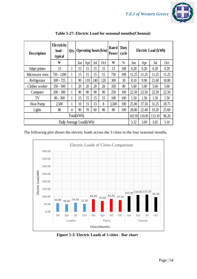
T.E.I of Western Greece
Page | 54
Table 5-27: Electric Load for seasonal months(Chennai)
Figure 5-3: Electric Loads of 3 cities - Bar chart
Electricity
load -
typical
Qty.Rated
Power
Duty
cycle
W Jan Apr Jul Oct W % Jan Apr Jul Oct
Inkjet printer 13 1 15 15 15 15 13 100 0.20 0.20 0.20 0.20
Microwave oven 750 - 1200 1 15 15 15 15 750 100 11.25 11.25 11.25 11.25
Refrigerator 300 - 725 1 90 110 240 120 300 30 8.10 9.90 21.60 10.80
Clothes washer 350 - 500 1 20 20 20 20 350 80 5.60 5.60 5.60 5.60
Computer 200 - 300 1 90 90 90 90 250 100 22.50 22.50 22.50 22.50
TV 80 - 300 1 15 15 15 15 100 100 1.50 1.50 1.50 1.50
Heat Pump 2,500 1 10 15 13 8 2,500 100 25.00 37.50 31.25 18.75
Lights 80 4 90 70 60 80 80 100 28.80 22.40 19.20 25.60
102.95 110.85 113.10 96.20
3.32 3.69 3.65 3.10
Operating hours(h/m) Electric Load (kWh)
Daily Average Load(kWh)
Total(kWh)
Description
56.80 49.6059.56 52.30
82.4070.40
84.20 77.10
102.95 110.85 113.1096.20
0.00
50.00
100.00
150.00
200.00
250.00
300.00
350.00
400.00
Jan Apr Jul Oct Jan Apr Jul Oct Jan Apr Jul Oct
London Patras Chennai
Ele
ctri
c Lo
ad,k
Wh
Cities/Months
Electric Loads of Cities-Comparison
The following plot shows the electric loads across the 3 cities in the four seasonal months.
T.E.I of Western Greece
Page | 55
SIZING OF RENEWABLE SYSTEMS FOR LOADS
The different options by which the loads(thermal and electric)calculated in the previous chapter
can be satisfied by using Renewable systems are as follows :
1.Solar Collector (Space Heating and Domestic Hot Water)
2. a) Heat Pump (Space Heating ,Domestic Hot Water and Cooling)
b) Heat Pump assisted by Solar Collector (Space Heating ,Domestic Hot Water and Cooling)
3. Absorption Chillers
4. a) Photo-Voltaics (Stand alone or Grid Connected)
b) PV/T
6.1 Calculation of Output of the Solar Collector
One of the options to meet the thermal loads is by the use of solar collectors.The design
of the solar collector is made considering the month where the maximum thermal load is to be
satisfied.It can be seen from Table 5-24 that for London,the thermal load demand is maximum
for January with a value of 4872.61 kWh.
For the purpose of this analysis, the solar collector that is considered to meet the thermal
loads is a flat plate solar collector(Manufacturer WOLF GmbH) which has the following
properties .
Table 6-1:Properties of Flat plate solar Collector
Parameter Value
Aperture Area 2m2 per collector
Overall Area 2.3m2 per collector
Brand Name Topson
Model Number F3-1

T.E.I of Western Greece
Page | 56
Heat Losses
Coefficient,FRUL 4.3 W/m2.oC
Optical Efficiency,FR(τα) 0.82
Absorber Solid copper with highly selective coating for very high yield
Insulation Mineral Thermal Insulation(60mm thick)
Application Hot water,Space Heating,pool etc.,
A daily simulation was performed to calculate the Solar Collector output.The following
equations were utilized to assist the calcuation.
𝑞𝑢,𝛥𝜏 = 𝐹𝑅
′ .[𝐻𝑛(𝜏𝛼) − 𝑈𝐿 . (𝑇𝑠,𝑖 − 𝑇𝑎). 𝛥𝜏]
1 + 𝐹𝑅′ .
𝑈𝐿
(2. 𝑚. 𝐶𝑝)𝑠
. 𝛥𝜏
6-1
𝑇𝑠,𝑓 = 𝑇𝑠,𝑖 +𝑞𝑢,𝛥𝜏
2. (𝑚. 𝐶𝑝)𝑠
6-2
qu,Δτ is the thermal output stored into the tank by the fluid flow per unit area of the
Solar Collector system.
Hn is the solar radiation intensity for the interval.
Ts,i is the temperature of water in the tank at the beginning of the time period τ and Ts,f
is the corresponding temperature at end of the period (τ + Δτ)
Τa is the average ambient temperature during the time interval (τ,τ + Δτ)
m is the capacity of the Hot water tank.

T.E.I of Western Greece
Page | 57
Flat plate
Collector
Area(m2)
F R U L (
W/m2
K)
F R (τα)
Optimal
angle of
inclination for
January(deg)
Temperature
of the tank at
8:30AM(o
C)
2 4.3 0.82 68 20
Hour T a (o
C) H T (KJ/m2) q u (KJ/m
2) T si (
oC) T sf (
oC) η = q u /H T
8:30AM-9:30AM 4 500.4 156.84 20.00 20.38 0.31
9:30AM-10:30AM 4.5 770.4 372.20 20.38 21.27 0.48
10:30AM-11:30AM 5.6 933.3 504.13 21.27 22.47 0.54
11:30AM-12:30PM 6.5 986.4 541.55 22.47 23.77 0.55
12:30PM-1:30PM 7 933.3 487.69 23.77 24.93 0.52
1:30PM-2:30PM 6.8 770.4 338.48 24.93 25.74 0.44
2:30PM-3:30PM 6.5 500.4 108.42 25.74 26.00 0.22
Total Solar Collector Output per
day(KJ/m2)
Total Solar Collector Output for the
month(kWh)
Hot water Tank
Capacity(kg/m2)
50
2509.30
43.22
Table 6-2: Monthly Output of the Solar Collector (London)
In Table 6-2,the values of the Heat Losses coefficient,FRUL and the optical
efficiency,FR(τα)are manufacturer values for the Flat plate solar collector.The optimal angle of
inclination was obtained from PVGIS database for the month of January.The initial temperature
of the water inside the tank and the capacity of the hot water tank were assumed to be 20oC and
50kg/m2 respectively.The ambient temperatures in column 2 of Table 6-2 were obtained from
PVGIS .By means of equations 6-1 and 6-2 all the corresponding values for each of the
parameters were calculated.The Solar collector output per day was obtained by the summation
of the hourly values of solar collector output.Finally, the solar collector output was determined
for the month of January for London.
The procedure in the above paragraph is repeated to determine the output of the solar
collector located in Patras and the results are tabulated in Table 6-3.

T.E.I of Western Greece
Page | 58
Flat plate
Collector
Area(m2)
F R U L (
W/m2
K)
F R (τα)
Optimal
angle of
inclination
for
January(deg)
Temperature
of the tank at
7:30AM(o
C)
2 4.3 0.82 61 20
Hour Ta(oC) HT(KJ/m
2) qu(KJ/m
2) Tsi (
oC) Tsf (
oC) η = qu/HT
7:30AM-8:30AM 9.6 561.6 288.82 20.00 20.69 0.51
8:30AM-9:30AM 11.5 1335.6 918.89 20.69 22.89 0.69
9:30AM-10:30AM 12.3 1888.2 1334.96 22.89 26.08 0.71
10:30AM-11:30AM 12.4 2234.7 1562.77 26.08 29.82 0.70
11:30AM-12:30PM 12.6 2350.8 1601.75 29.82 33.65 0.68
12:30PM-1:30PM 12.3 2234.7 1448.27 33.65 37.12 0.65
1:30PM-2:30PM 12 1888.2 1118.09 37.12 39.79 0.59
2:30PM-3:30PM 11.5 1335.6 633.74 39.79 41.31 0.47
3:30PM-4:30PM 10.9 621.9 37.82 41.31 41.40 0.06
Total Solar Collector Output per
day(KJ/m2)
Total Solar Collector Output for the
month(kWh)
Hot water Tank
Capacity(kg/m2)
50
8945.11
154.05
Table 6-3: Monthly Output of the Solar Collector(Patras)
Following the calculation of the solar collector output, the collector area(m2) required
for meeting a definite fraction of the thermal load,f of January can now be computed. This is
obtained by calculating the thermal load corresponding to each fraction and dividing the value
by the solar collector output of the corresponding city.The results for both cities are given in
Table 6-4.
Table 6-4:Collector Area and quantity of Collectors(London & Patras)
S.No
% of Thermal loads
met by Solar
Collector(Space
heating +Hot water
+ Heat Losses)
Minimum Collector
Area(m2) required for
Covering the Loads
No. of Collectors(Rounded
off to nearest whole
number)
London Patras London Patras
1 30 23 6 12 3
2 40 34 9 17 5
3 50 45 11 23 6
4 60 56 13 28 7
5 70 68 15 34 8

T.E.I of Western Greece
Page | 59
6 80 79 17 40 9
7 90 90 19 45 10
8 100 101 21 51 11
6.2 Cooling Equipment selection for Cooling Loads(Chennai)
One of the options to meet the cooling demand is by use of Heat Pumps.This section
outlines the procedure involved in the selection of the appropriate Heat Pump. The Heat Pump
is an air source Heat Pump. Air source heat pump systems are not a common choice in cold
climates with a large heating load.However, an air source heat pump is a likely choice for
climates where the heating load is much smaller than the cooling load i.e., for cases like
Chennai .
As seen from Fig.6-1,the primary step is to define the design parameters.Since the heat
pump selection is made based on the month which has the maximum cooling Load for Chennai
i.e., April . The design cooling load is the amount of heat energy to be removed from a house
by the HVAC equipment to maintain the house at indoor design temperature when worst case
outdoor design temperature is being experienced.
There are two types of cooling loads namely Sensible Cooling Load and Latent Cooling
Load. The sensible cooling load refers to the dry bulb temperature of the building and the latent
cooling load refers to the wet bulb temperature of the building.The Latent Cooling load is
considered to be 30% of the total cooling Load(Manual S) and the values given in the following
table are that at Solar noon for April (Refer Table 5-23).The other design parameters are also
defined based on the considered region(in this case Chennai).
Figure 6-1: Cooling equipment selection steps
(Source : Manual S,2013)

T.E.I of Western Greece
Page | 60
Loads
Heating Load Nil
Sensible Cooling Load 19319.47 Btu/hr (5661.97W/hr)
Latent Cooling Load 1179.727 Btu/hr (345.74W/hr)
Outdoor
Conditions
Cooling-Dry Bulb Temperature 87.62oF (30.9 oC)
Heating Dry-Bulb Temperature 2oF (-16.67 oC)
Indoor Conditions
Cooling-Dry Bulb Temperature 72oF (22oC)
Cooling-Wet Bulb Temperature 63oF (17 oC)
Heating Dry-Bulb Temperature 66oF (18.8 oC)
Air flow Estimates Cubic Feet per minute(cfm) To be determined
To search the manufacturer’s expanded performance data, an initial estimate of the
required cfm airflow is needed. The estimated cfm airflow is used only to narrow down the
equipment choices from the manufacturer’s data and will likely be higher than the actual cfm
used for the design.
The detailed procedure to estimate a target cfm is described in Manual S. Manual S
instructs the designer to use the Sensible Heat Ratio (SHR) value to determine the desired
room-air to supply-air Temperature Difference (TD) in degrees Fahrenheit.
𝑆𝐻𝑅 =
𝑆𝑒𝑛𝑠𝑖𝑏𝑙𝑒 𝐿𝑜𝑎𝑑
𝑇𝑜𝑡𝑎𝑙 𝐿𝑜𝑎𝑑 6-3
Manual S shows the relationship of an SHR range to TD value that is compatible with the
sensible and latent loads. The column “LAT” is the temperature of air leaving the coil, and the
column “Room db” is the indoor conditions dry-bulb temperature .The difference between the two
is the TD value.
Table 6-5: TD Value (from Manual S)
Sensible Heat Ratio versus TD Value
SHR LAT(oC) Room db(oC) TD(oC)
Below 0.80 53 75 22
0.80 to 0.85 55 75 20
Above 0.85 57 75 18

T.E.I of Western Greece
Page | 61
Once the TD value is known, the estimated cfm target can be calculated using equation 6-4
𝑐𝑓𝑚 𝑇𝑎𝑟𝑔𝑒𝑡 =
𝑆𝑒𝑛𝑠𝑖𝑏𝑙𝑒 𝐿𝑜𝑎𝑑
1.1 𝑋 𝑇𝐷 6-4
The number 1.1 in the denominator of equation 6-4 represents an air properties constant
associated with elevations lower than 1,500 feet.Since Chennai is located at an elevation of
200ft the above constant is appropriate.
From equation 6-3
SHR = (Sensible Load/Total Load) = (19319.47Btu/hr/20499.197Btu/hr) = 0.94
From the TD value Table 6-5, the TD value for SHR = 0.94 is 18 .Using these values in equation
6-4 ,the cfm target is :
Cfm target = Sensible Load/(1.1 X TD) = (19319.47/1.1*18) = 975.73
Step 3, highlighted in Fig. 6-1, is to search the manufacturer’s data for an adequate
cooling equipment package. Considering that 12000 Btu/h is equivalent to 1 nominal ton of
cooling, the 20499.1997 Btu/h total cooling load for the building in Chennai leads to a 2-ton
nominal size cooling system as the target size to begin the equipment search.
The Entering Wet-Bulb Temperature(EWB) temperature for the indoor coil can be
determined on the sea-level psychometric chart for our reference conditions of 22oC~72°F
indoor design dry-bulb temperature and 62.5% relative humidity for April(Refer Table II-A of
Appendix II), as shown in Fig. 6-2.
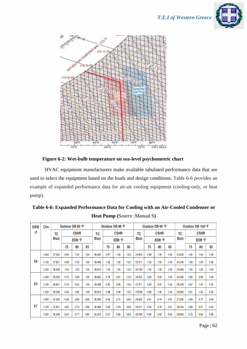
T.E.I of Western Greece
Page | 62
Figure 6-2: Wet-bulb temperature on sea-level psychometric chart
HVAC equipment manufacturers make available tabulated performance data that are
used to select the equipment based on the loads and design conditions. Table 6-6 provides an
example of expanded performance data for air-air cooling equipment (cooling-only, or heat
pump).
Table 6-6: Expanded Performance Data for Cooling with an Air-Cooled Condenser or
Heat Pump (Source :Manual S)

T.E.I of Western Greece
Page | 63
In Table 6-6,EWB = Entering Wet Bulb Temperature ,EDB = Entering Dry Bulb
Temperature, Cfm = Blower Cfm setting ,TC = Total cooling capacity (sensible plus latent),
CSHR = Coil sensible heat ratio = Sensible Btuh / Total Btuh
In Chennai ,the EWB as determined on the sea level psychrometric chart(Fig.6-2) is
63oF, Outdoor DBT is 87.5oF ~ 90oF ,Indoor DBT is 72oF ~ 75oF and the blower cfm is 975
which is closer to 1000 in Table 6-6 .
Hence the total Cooling Capacity required for the Heat Pump = 26,955 Btuh = 7.9kWh ~ 8kWh
The Coefficient of Performance of the selected Heat Pump is given by the following equation:
𝐶𝑂𝑃 =𝐶𝑜𝑜𝑙𝑖𝑛𝑔 (𝑜𝑟 𝐻𝑒𝑎𝑡𝑖𝑛𝑔)𝑝𝑟𝑜𝑣𝑖𝑑𝑒𝑑
𝑊𝑜𝑟𝑘 𝐶𝑜𝑛𝑠𝑢𝑚𝑒𝑑 𝑏𝑦 𝐻𝑒𝑎𝑡 𝑃𝑢𝑚𝑝 6-5
A Heat Pump with a cooling capacity of 8kWh will have a rated electrical power
consumption by Fan coils,Compressor etc., of 2.5kWh (Source :Energy.Gov) .Hence the COP
of the Heat Pump will be :
COP = 8/2.5 = 3.2
6.3 Sizing of Stand-alone PV for meeting the Electric Loads
To design a stand-alone PV system required to cover the electric Loads of the Building the
following steps are required .
Step 1:
The scenario for which the PV System has to cover the daily energy demand,the electrical
appliances and their daily hours of operation and months of usage are decided.The Stand-alone
PV system has been sized in Chennai for the month with the maximum electric Load and the
worse month in terms of Solar-irradiation(Nov).
Step 2 :
The appliances that are used in the building along with their rated power and operating hours
are entered to determine the daily Load QL are in Table 5-27.
As seen from Table 5-27,the monthly electricity consumption for April is 110.85kWh and
hence the daily load, QL is 3.69kWh.
Note :The operating hours of all the appliances are given in hours per month .

T.E.I of Western Greece
Page | 64
Step 3 :
The PV installation details are decided.The building under consideration is located in an open
ground with minimal obstacles/objects.Hence the effects of shading are ignored.
A free PV system is choosen over a BIPV.
The optimal inclination angle of the PV for maximum incident solar radiation throughout the
year is 15o and the daily irradiation on the horizontal is 5690W/m2.The above values are
obtained from PVGIS database as shown :
Table 6-7: Irradiation on the Horizontal and Optimal inclination angle for Chennai
(Source :PVGIS)
Step 4 :
The average Peak Solar Hours (PSH)of the day are determined for the worse month in terms
of incident solar energy.PSH is defined as the time length in hours/day for a given day such
that the solar intensity is constant at 103W/m2.The PSH value will be such that

T.E.I of Western Greece
Page | 65
Table 6-8: Irradiation at the Optimal inclination angle for Chennai
(Source : PVGIS)
H = (PSH)h/day.103W/m2 .It can be seen from Table 6-7 that the average PSH for the worse
month of sizing (November) is 4.54hrs.
The average conversion factor ,R of the solar radiation from the horizontal to the inclined is
calculated.
HT avg= Havg . Ravg 6-6
Ravg = HT avg/ Havg = 5060/4540
Ravg = 1.114
The PSHavg.Ravg is determined through the mean monthly daily solar irradiation HTavg obtained
from PVGIS for the worse month (November) and is
PSHavg.Ravg = (4.54x1.114) = 5.06

T.E.I of Western Greece
Page | 66
Step 5:
The autonomy factor d for the non-critical loads considered in step 2 is determined.In this
scenario, the loads are all non-critical and hence it is satisfactory if the demands are met 95%
of the time .
dn-cr = -0.48*PSH min + 4.58(days) 6-7
The minimum PSH of the sizing month is obtained from SoDa Database for a period of 10-15
years(Refer Table II-A ,Appendix II).It is to be noted here that the mean monthly daily value
of irradiation for the sizing month November is given in J/Cm2 i.e.,1642 J/Cm2.Hence the value
is converted to Wh/m2 by multiplying by 2.778 .
Hence PSHmin = 1642*2.778/1000 = 4.56hrs/day
Hence dn-cr = -0.48*4.56 + 4.58(days)
dn-cr = 2.39 ~ 3 days
Step 6 :
The installed Peak power Pm is determined :
(𝑃𝑚 + 𝛿𝑃𝑚)𝑃𝑆𝐻𝑎𝑣𝑔. 𝑅𝑎𝑣𝑔. 𝜂𝑖𝑛𝑣. 𝜂𝑐ℎ. 𝜂𝑐𝑎𝑏 . 𝜂𝑏𝑎𝑡 = 𝑄𝐿 . 𝑑 6-8
Typical Values ηinv = 95%, ηbat = 85%, ηch = 95%, ηcab = 98%
δPm due to the temperature developed in the PV is calculated :
PV Temperature TPV is estimated through the following expression.
TPV = Ta + f.IT 6-9
Where f=0.03oC/(W/m2) for free standing PV system.The values of Ta and IT for the sizing
month are determined from PVGIS by considering Clear Sky Global Irradiance and finding the
average of irradiance and temperature at 12,12 – PSH /2 and 12+PSH/2 from the mean monthly
hourly profile of solar irradiance and ambient temperature respectively as shown in Fig.6-3.

T.E.I of Western Greece
Page | 67
Figure 6-3:Irradiance profile(daily)for Chennai
(Source : PVGIS)
The values of Ta and IT were calculated as 26.1oC and 853.33W/m2
TPV = 26.1+ 0.03*853.33
TPV = 51.7oC
The temperature coefficient of power is assumed to be -0.45%/ oC
(δPm/Pm) = -0.0045(51.7-26.1)
(δPm/Pm) = -0.1152 => δPm = -0.115Pm
Substituting the above in equation 6-8
(Pm-0.115Pm)*5.06*0.95*0.95*0.98*0.85 = 3.69*103*3
0.885Pm = 2910.083
Pm = 3288.23 W = 3.29kW
Step 7 :
The installed Battery Capacity is determined by equation 6-10,

T.E.I of Western Greece
Page | 68
Table 6-9:Annual Stand alone PV performance with days of autonomy 3
C = (d.QL)/(V.DOD.ηinv-ch.ηbat) 6-10
= 3*3.69*103/(24*0.80*0.95*0.85)
C = 714 Ah
The batteries are located in a room where the temperature is 25oC.Hence the correction factor
is 1.
Step 8 :
The performance of the stand-alone PV system designed is checked in PVGIS Database by
entering the values of the installed peak power Pm , battery capacity C and average daily load
QL estimated for the sizing month(November) .The following results were obtained :
As seen from Table 6-9 ,the system appears to be over-sized since there are no failures.It may
be noted that a system failure of upto 5% for non-critical loads is permissible.
Hence, the days of autonomy d is reduced from 3 to 2 and the installed Peak Power Pm and the
battery capacity C are calculated again.
(Pm - 0.115Pm)*5.06*0.95*0.95*0.98*0.85 = 3.69*103*2

T.E.I of Western Greece
Page | 69
Table 6-10:Annual Stand alone PV performance with days of autonomy 2
0.885Pm = 1940.043
Pm = 2192.15 W = 2.19 kW
Battery Capacity, C = 2*3.69*103/(24*0.80*0.95*0.85)
C = 476 Ah
The above values are again entered in PVGIS to check the failure rate of the Stand-alone PV
System(SAPV)and the following was obtained :
As seen from Table 6-10,the total system failure is 2% .As the load is non-critical ,the choosen
values are optimal.
Note: It is to be mentioned here that as the appliances are arbitrarily decided, the hourly
consumption profile is not known and the default night-based hourly consumption profile of
PVGIS as shown in Fig.6-4 is utilized in the above scenario.
Step 9 :
For the final estimated Pm and C,the number of PV modules and batteries to be connected are
determined .
a)Bio-195 module is choosen and the number of modules NPV required are calculated .
NPV = Pm,gen/Pm,module = 2192.15/195
= 11.24 ~ 12

T.E.I of Western Greece
Page | 70
The number of modules to be connected in series is calculated based on the DC voltage V for
Power Transfer .
Npv,s = V/Vm
Temperature coefficient of Voltage for the above module is -0.1801 V/°C(as provided by the
manufacturer) .Hence the Voltage Vm corrected to the temperature of the PV module is
Vm = 36.94 – 0.1801*(51.7 – 25)
Vm = 32.13V
Therefore, NPV,S = 24/32.13 = 0.747 ~ 1
The number of strings to be connected in parallel is Npv,p = Npv / Npv,s
Npv,p = 12/1 = 12
b)12V 100AH Lithium Ion batteries are selected with DOD 80%
The number of batteries to be connected in series ,Nb,s = V/Vb =24/12
Nb,s = 2
The number of strings to be connected in parallel are Nb,p =C/Cb = 476/100
Nb,p = 4.76 ~ 5
The corrections due to the charge/discharge rate are calculated
fb,ch/disch = ich/disch(as recommended)/ich,disch(due to the load profile) 6-11
The recommended upper value for charge/discharge is C/10 = [5*100]/10 = 50 A
The hourly profile of the appliances is given below :

T.E.I of Western Greece
Page | 71
Figure 6-4:Hourly Consumption profile of the selected Loads
From the default hourly load profile as obtained from PVGIS,the maximum value of discharge
current is found to be 0.1175*3.69*103/(24*0.95) = 19.01A which is less than the
recommended value of discharge.
However, the rate of charging is (number of panels *Im of the module) = 12*5.28 = 63.36A
which is more than the recommended value of charging.Hence a correction factor is imposed
fb,ch/disch = 50/63.36 = 0.789
The Corrected Battery Capacity Ccor = 476/0.789 = 603.29Ah
Ccor = 603.29 Ah
Therefore the actual number of Battery strings in parallel is 603.29/100 = 6.03 ~ 6
Step 10 :
The stand-alone PV system has been designed for the scenario considered and the following
are the sizing details for the installation in Chennai :

T.E.I of Western Greece
Page | 72
Table 6-11: Stand alone PV system chennai design details
General Battery Details PV Panel details
Installed Peak
Power,Pm=
2.19kW
Total
Capacity(Corrected),
C 600 Ah
Total Number
of Panels,NPV 12
Days of
Autonomy,d=2
Number of Batteries
in series,Nb,s 2
Number of
Panels in
series,Npv,s 1
Number of Battery
strings in parallel,
Nb,p 6
Number of
Strings in
Parallel, Npv,p 12
Battery 12V 100AH Lithium Ion
Module Bio-195(Peak
Power 195W)
The above procedure is also adopted for the building in London and Patras and the sizing details
tabulated as follows :
Table 6-12: Stand alone PV system(London) design details
General Battery Details PV Panel details
Installed Peak
Power,Pm= 8.8kW
Total
Capacity(Corrected),
C 2400 Ah
Total Number
of Panels,NPV 46
Days of
Autonomy,d=4
Number of Batteries
in series,Nb,s 2
Number of
Panels in
series,Npv,s 1
Number of Battery
strings in parallel,
Nb,p 24
Number of
Strings in
Parallel, Npv,p 46
Battery 12V 100AH Lithium Ion
Module Bio-195(Peak
Power 195W)
Table 6-13:Stand alone PV system(Patras) design details
General Battery Details PV Panel details
Installed Peak
Power,Pm= 3.8 kW
Total
Capacity(Corrected),
C 1000 Ah
Total Number
of Panels,NPV 20
Days of
Autonomy,d=3
Number of Batteries
in series,Nb,s 2
Number of
Panels in
series,Npv,s 1
Number of Battery
strings in parallel,
Nb,p 10
Number of
Strings in
Parallel, Npv,p 20
Battery 12V 100AH Lithium Ion
Module Bio-195(Peak
Power 195W)

T.E.I of Western Greece
Page | 73
6.4 Sizing of Stand-alone PV using a stochastic approach
An extensive,thorough and in-depth analysis comprising hourly data for each of the
days and for all days in the month of December was carried out for London ,Patras and
November for Chennai .The sizing of the PV was done considering these months since this is
the worse month in terms of solar radiation for the respective city and if the PV system is
designed to meet the loads for this month,it is more likely to meet the loads for the other months
where the solar radiation is better.The following equations were utilized in the analysis(Kaplani
and Kaplanis 2012) .
𝐼𝑇 = 𝐼. 𝑅 6-12
𝑅 = (1 −
𝐼𝑑
𝐼) . 𝑅𝑏 +
𝐼𝑑
𝐼.1 + 𝐶𝑜𝑠(𝛽)
2+ 𝑟.
1 − 𝐶𝑜𝑠(𝛽)
2
6-13
𝐸𝑃𝑉 = 𝑃𝑚,𝑐𝑜𝑟. 𝑃𝑆𝐻. 𝑅 6-14
𝐷𝐸 = 𝐸𝑃𝑉 − 𝐹. 𝑄𝐿𝑑𝑎𝑦 6-15
𝑆𝑂𝐶 = 𝑆𝑂𝐶𝑎 +
𝐷𝐸
𝐶𝐿 . 𝑉
6-16
𝐸𝑙𝑜𝑠𝑠 = (𝑆𝑂𝐶 − 1). 𝐶𝐿 . 𝑉 6-17
𝑆𝑂𝐶 = 𝑆𝑂𝐶𝑎 −
𝑄𝐿𝑛𝑖𝑔ℎ𝑡. 𝐹′
𝐶𝐿 . 𝑉 6-18
Where
ΙΤ is the intensity on the PV plane at the optimal angle of inclination
R is the conversion factor for the solar radiation from the horizontal to the inclined PV array
EPV is the energy delivered by the PV (Wh)
Pm,cor is the corrected Peak power of the PV (Wp)
PSH is the Peak Solar Hour

T.E.I of Western Greece
Page | 74
DE is the remaining amount of the energy delivered after its consumption by the loads
SOC is the state of charge of battery(%)
SOCa is the remaining SOC carried onto the subsequent hour
CL is the battery capacity (Ah)
V is the DC transfer voltage
QLday,QLnight are the hourly loads with the former denoting loads during the time the PV
produces energy and the latter when the PV does not produce energy and the battery meets the
loads
Eloss is the energy burnt by a damp load due to excess energy and fully charged battery (Wh)
Since the analysis is hourly,all the terms in the equations (6-12) to (6-18) denote hourly values.
6.4.1 Simulation Methodology
The hourly values of Global Solar Radiation intensity,I(W/m2),Diffuse Solar Radiation
Intensity,Id(W/m2), ambient temperature,Ta(oC) are downloaded from a database(in this case
Meteonorm) for all the days in December(November for Chennai).The Beam Solar Radiation
Intensity,Ib(W/m2) can then be calculated by means of equation (5-12) .
Next,the intensity on the inclined plane,IT has to be determined . The optimal angle of
inclination is that which gives the maximum output when considered on an yearly basis.This
value for London was obtained from PVGIS and is 38o .The intensity on the PV plane at this
angle of inclination(IT) is given by equation (6-12).
The installed peak power of the PV(Pm) is initially assumed to be 1 kW or the initial
assumed value may also be calculated by equation (6-8) with d = 1.In our case,the value is
initially assumed to be 1kW.The battery capacity ,CL is calculated by means of equation 6-10
wherein the days of autonomy,d is considered to be unity and the load QL is the average daily
load of the seasonal month with the maximum load.
The performance of the PV is simulated for the entire month for each hour in a platform
(in this case MS - EXCEL)and the number of hours of failure i.e., the number of hours the state
of charge of the Battery goes below (1-DOD)or in other words less than 20% is determined.For
non-critical loads ,the percentage of failure as stated in section 6.3 has to be less than 5%.In

T.E.I of Western Greece
Page | 75
this stochastic approach,the percentage of failure is calculated by dividing the number of hours
in which the battery SOC goes below 20% by the total number of hours for the month of
December which is 744 (31X24).
In case the failure is less than 5%,the peak power Pm is suitably altered until the failure
is just below 5%.If the failure is more than 5%,the peak power of the Pm is increased in steps
of 0.5kW and for each of this increase the battery capacity is proportionately increased from
the original calculated value (with d=1).For instance if the peak power is doubled from the
1kW to 2kW,the battery capacity is also doubled .
For each of these instances, the failure rate for the total month is calculated and the
analysis is continued until the selected value of peak power and the corresponding battery
capacity produces a failure rate no more than 5% throughout the month.The Peak power may
also be increased in steps of 0.25kW (or even smaller) and the battery capacity,CL
proportionately increased until the failure rate becomes no more than 5%.This final value of
Peak Power,Pm and the Battery Capacity,CL represent the sizing of the PV system.
Table 6-14 ,6-15 and 6-16 shows the values of energy produced by the PV(EPV) , the
delivered energy(DE),state of charge of the Battery(SOC), the energy burnt by a damp
load(Eloss) etc., calculated for a typical day (n = 11) for different values of Peak Power (Pm)
and Battery Capacity (CL) for London.Tables IV-A and IV-B in Appendix IV shows the above
mentioned entities for Patras and Chennai respectively during a typical day.

T.E.I of Western Greece
Page | 76
Hour
Ambient
Temperature
,Ta(oC)
Global
Solar
Radiation
Intensity,I
(W/m2)
Diffuse
Solar
Radiation
Intensity,I
d(W/m2)
Intensity
on the
inclined
plane,IT(
W/m2)
Night based
consumption
profile
fractions(PV
GIS)
Hourly
Load,(
W)
Peak
power
corrected
for
temperat
ure,(Wp)
Energy
produce
d by
PV,EPV(
Wh)
Delivere
d
Energy,
DE(Wh)
State of
Charge of
Battery,S
OC(%)
Energy
burnt,Elos
s(Wh)
1 11.5 0 0 0 0.0505 92.415 1500 0 0 -1.30 0
2 11.5 0 0 0 0.035 64.05 1500 0 0 -3.17 0
3 11.3 0 0 0 0.027 49.41 1500 0 0 -4.61 0
4 10.6 0 0 0 0.025 45.75 1500 0 0 -5.94 0
5 9.5 0 0 0 0.0245 44.835 1500 0 0 -7.25 0
6 8.5 0 0 0 0.0265 48.495 1500 0 0 -8.66 0
7 9.3 0 0 0 0.0345 63.135 1500 0 0 -10.50 0
8 8.8 0 0 0 0.0295 53.985 1500 0 0 -12.08 0
9 8.5 29 26 73.82 0.023 42.09 1485.05 109.62 50.88 -10.94 0
10 9.4 124 72 368.77 0.018 32.94 1425.32 525.62 479.65 -0.18 0
11 10.1 161 88 400.37 0.018 32.94 1418.92 568.10 522.13 11.53 0
12 11.6 266 114 707.50 0.0205 37.515 1356.73 959.89 907.53 31.89 0
13 11.6 198 97 489.11 0.0265 48.495 1400.95 685.22 617.54 45.74 0
14 11.5 181 74 537.69 0.035 64.05 1391.12 747.99 658.60 60.51 0
15 11.2 111 44 431.55 0.0415 75.945 1412.61 609.61 503.63 71.81 0
16 10.2 23 23 20.56 0.0505 92.415 1495.84 30.76 -98.22 69.61 0
17 8.5 0 0 0 0.0455 83.265 1500 0 0 67.18 0
18 7.8 0 0 0 0.034 62.22 1500 0 0 65.37 0
19 7.1 0 0 0 0.025 45.75 1500 0 0 64.04 0
20 6.6 0 0 0 0.03 54.9 1500 0 0 62.44 0
21 6 0 0 0 0.065 118.95 1500 0 0 58.97 0
22 6.1 0 0 0 0.1095 200.39 1500 0 0 53.13 0
23 5.7 0 0 0 0.1175 215.03 1500 0 0 46.86 0
24 4.6 0 0 0 0.088 161.04 1500 0 0 42.17 0
Table 6-14:PV Simulation values on a typical day(n=11) for Peak Power Pm = 1.5 kW and
Battery Capacity ,CL = 186Ah // London(December)
The rate of failure for this instance of simulation (Pm = 1.5 kW,CL=186Ah) was very
high and found to be 84.94%(i.e.,698 hrs failure out of 744 hrs)
Note : A negative value of SOC implies that the state of charge of the Battery is zero .

T.E.I of Western Greece
Page | 77
Hour
Ambient
Temperature
,Ta(oC)
Global
Solar
Radiation
Intensity,I
(W/m2)
Diffuse
Solar
Radiation
Intensity,I
d(W/m2)
Intensity
on the
inclined
plane,IT(
W/m2)
Night based
consumption
profile
fractions(PV
GIS)
Hourly
Load,(
W)
Peak
power
corrected
for
temperat
ure,(Wp)
Energy
produce
d by
PV,EPV(
Wh)
Delivere
d
Energy,
DE(Wh)
State of
Charge of
Battery,S
OC(%)
Energy
burnt,Elos
s(Wh)
1 11.5 0 0 0 0.0505 92.415 2000 0 0 76.67 0
2 11.5 0 0 0 0.035 64.05 2000 0 0 75.27 0
3 11.3 0 0 0 0.027 49.41 2000 0 0 74.19 0
4 10.6 0 0 0 0.025 45.75 2000 0 0 73.19 0
5 9.5 0 0 0 0.0245 44.835 2000 0 0 72.21 0
6 8.5 0 0 0 0.0265 48.495 2000 0 0 71.15 0
7 9.3 0 0 0 0.0345 63.135 2000 0 0 69.77 0
8 8.8 0 0 0 0.0295 53.985 2000 0 0 68.59 0
9 8.5 29 26 73.82 0.023 42.09 1980.07 146.16 90.17 70.18 0
10 9.4 124 72 368.77 0.018 32.94 1900.43 700.83 657.01 81.78 0
11 10.1 161 88 400.37 0.018 32.94 1891.90 757.46 713.65 94.37 0
12 11.6 266 114 707.50 0.0205 37.515 1808.98 1279.85 1229.95 100.00 911.17
13 11.6 198 97 489.11 0.0265 48.495 1867.94 913.63 849.12 100.00 849.12
14 11.5 181 74 537.69 0.035 64.05 1854.82 997.31 912.12 100.00 912.12
15 11.2 111 44 431.55 0.0415 75.945 1883.48 812.82 711.80 100.00 711.80
16 10.2 23 23 20.56 0.0505 92.415 1994.45 41.01 -81.92 98.55 0
17 8.5 0 0 0 0.0455 83.265 2000 0 0 96.73 0
18 7.8 0 0 0 0.034 62.22 2000 0 0 95.37 0
19 7.1 0 0 0 0.025 45.75 2000 0 0 94.37 0
20 6.6 0 0 0 0.03 54.9 2000 0 0 93.17 0
21 6 0 0 0 0.065 118.95 2000 0 0 90.57 0
22 6.1 0 0 0 0.1095 200.39 2000 0 0 86.19 0
23 5.7 0 0 0 0.1175 215.03 2000 0 0 81.49 0
24 4.6 0 0 0 0.088 161.04 2000 0 0 77.97 0
Table 6-15 : PV Simulation values on a typical day(n=11) for Peak Power Pm = 2kW and Battery
Capacity ,CL = 236Ah // London(December)
The rate of failure for this instance of simulation (Pm = 2kW,CL=236Ah) was 65.59%
(i.e.,.496 hrs failure out of 744 hrs).

T.E.I of Western Greece
Page | 78
Hour
Ambient
Temperature
,Ta(oC)
Global
Solar
Radiation
Intensity,I
(W/m2)
Diffuse
Solar
Radiation
Intensity,I
d(W/m2)
Intensity
on the
inclined
plane,IT(
W/m2)
Night based
consumption
profile
fractions(PV
GIS)
Hourly
Load,(
W)
Peak
power
corrected
for
temperat
ure,(Wp)
Energy
produce
d by
PV,EPV(
Wh)
Delivere
d
Energy,
DE(Wh)
State of
Charge of
Battery,S
OC(%)
Energy
burnt,Elos
s(Wh)
1 11.5 0 0 0 0.0505 92.415 4000 0 0 88.70 0
2 11.5 0 0 0 0.035 64.05 4000 0 0 88.00 0
3 11.3 0 0 0 0.027 49.41 4000 0 0 87.46 0
4 10.6 0 0 0 0.025 45.75 4000 0 0 86.96 0
5 9.5 0 0 0 0.0245 44.835 4000 0 0 86.47 0
6 8.5 0 0 0 0.0265 48.495 4000 0 0 85.94 0
7 9.3 0 0 0 0.0345 63.135 4000 0 0 85.25 0
8 8.8 0 0 0 0.0295 53.985 4000 0 0 84.66 0
9 8.5 29 26 73.82 0.023 42.09 3960.139 292.324 233.58 86.62 0
10 9.4 124 72 368.77 0.018 32.94 3800.862 1401.66 1355.7 98.03 0
11 10.1 161 88 400.37 0.018 32.94 3783.8 1514.92 1469 100.00 1234.52
12 11.6 266 114 707.50 0.0205 37.515 3617.951 2559.69 2507.3 100.00 2507.34
13 11.6 198 97 489.11 0.0265 48.495 3735.88 1827.26 1759.6 100.00 1759.58
14 11.5 181 74 537.69 0.035 64.05 3709.649 1994.63 1905.2 100.00 1905.24
15 11.2 111 44 431.55 0.0415 75.945 3766.962 1625.64 1519.7 100.00 1519.65
16 10.2 23 23 20.56 0.0505 92.415 3988.896 82.0202 -46.953 99.61 0
17 8.5 0 0 0 0.0455 83.265 4000 0 0 98.70 0
18 7.8 0 0 0 0.034 62.22 4000 0 0 98.02 0
19 7.1 0 0 0 0.025 45.75 4000 0 0 97.52 0
20 6.6 0 0 0 0.03 54.9 4000 0 0 96.92 0
21 6 0 0 0 0.065 118.95 4000 0 0 95.62 0
22 6.1 0 0 0 0.1095 200.39 4000 0 0 93.43 0
23 5.7 0 0 0 0.1175 215.03 4000 0 0 91.08 0
24 4.6 0 0 0 0.088 161.04 4000 0 0 89.32 0
Table 6-16:PV Simulation values on a typical day(n=11) for Peak Power Pm = 4kW and Battery
Capacity ,CL = 495 Ah // London(December)
The failure rate in this instance of simulation is 11.82%(i.e.,88 hrs failure out of 744
hrs) which is much lesser than the earlier 2 cases but still higher than the permissible limit of
5%.Finally, the failure rate was brought down to just less than 5% by increasing the Peak power
of the PV in smaller steps and was determined to be 4110W i.e., 4.1kW with the corresponding
Battery capacity,CL as 508.97Ah which after applying the correction factor (as explained in
section 6.3 of step 9 ) becomes 940.59Ah.As the peak power is increased with corresponding
increase in battery capacity the failure rate goes down.Also it can be observed from all instances
of simulation that for each increase of Peak power Pm ,the battery capacity CL was also
proportionately increased as explained earlier in the simulation methodology.

T.E.I of Western Greece
Page | 79
COST EFFECTIVE CONFIGURATION FOR SOLAR
COLLECTOR
In order to determine the fraction of thermal needs to be covered by the solar collector
that is economically attractive, 8 scenarios as presented in Table 7-1 are considered in Patras.
For each scenario the fraction of needs not met by the Solar Collector is achieved by the use of
Heating Oil .The ideal fraction of needs is decided based on the Internal Rate of Return(IRR)
and the Net Present value (NPV).
Table 7-1: Different fractions of thermal loads by solar collector
Scenario
% of Thermal loads met by Solar
Collector(Space heating +Hot water
+ Heat Losses)
% of Thermal loads covered by
Oil(Space heating +Hot water + Heat
Losses)
1 30 70
2 40 60
3 50 50
4 60 40
5 70 30
6 80 20
7 90 10
8 100 0
Internal rate of return (IRR) is the interest rate at which the net present value of all
the cash flows (both positive and negative) from a project or investment equal zero.The basic
formula for calculating IRR is :
𝑷𝟎 +
𝑷𝟏
𝟏 + 𝑰𝑹𝑹+
𝑷𝟐
(𝟏 + 𝑰𝑹𝑹)𝟐+
𝑷𝟑
(𝟏 + 𝑰𝑹𝑹)𝟑+ ⋯
𝑷𝒏
(𝟏 + 𝑰𝑹𝑹)𝒏= 𝟎
7-1
where P0, P1, . . . Pn equals the cash flows in periods 1,2,….n, respectively and
IRR equals the project's internal rate of return.The higher the IRR,the more it becomes
appealing for any situation.

T.E.I of Western Greece
Page | 80
Table 7-2:Costs for Solar Thermal Technologies
Net Present Value (NPV) is defined as the difference between the present value of cash
inflows and the present value of cash outflows. NPV is used in capital budgeting to analyse the
profitability of a projected investment of project.It is defined by the equation as given below :
𝑵𝑷𝑽 = − 𝑪𝑰 + ∑𝑪𝒊𝒏
(𝟏 + 𝒊)𝒏
𝑵
𝒕=𝟏
− ∑𝑪𝒐𝒖𝒕
(𝟏 + 𝒊)𝒏 7-2
Where
CI refers to the Capital investment cost
Cin refers to the cash inflows each year.
Cout refers to the cash outflows (maintenance etc.,)each year
i refers to the rate at which the cash flow is discounted each year
n refers to the number of years.
A positive Net present value(NPV) indicates that the projected earnings generated by a
project or investment exceeds the anticipated costs.Generally an investment with a positive
NPV will be profitable and one with a negative NPV will result in loss.This concept is the basis
for the Net Present Value,which dictates that the only investments that should be made are
those with positive NPV values.
To proceed with the economic analysis,it is important to have an idea about the capital
costs required for the solar collector and the operations & Maintenance costs(O&M).To this
end, the costs provided in Table 7-2 and Fig.7-1 which have been taken from NREL website
can be used as the reference.
(Source : NREL)

T.E.I of Western Greece
Page | 81
From Table 7-2, it can be noticed that the mean installed cost per Flat pate solar
collectors is $141/ft2 and the installed cost range is (+/- $82/ft2).For this analysis,the capital
costs of the Flat Plate Solar Collectors has been assigned the lower range i.e., $59/ft2 ($141/ft2
- $82/ft2 ) . $59/ft2 is equivalent to 54.41€/ ft2 (1$ = 0.9222€ based on the exchange rate as on
17/12/2015 when this analysis was performed).The above figure on further conversion to SI
units leads to a cost of 585.66 €/m2 (1m2 = 10.76ft2) of flat plate collector.The Operations &
Maintenance Cost (O&M) has been taken as 1% of the initial installed cost i.e., Capital Cost.
Figure 7-1: Installed Costs for Solar Thermal Technologies
(Source : NREL)
Table 7-3 shows the quantity of Heating Oil required in litres if it were used to satisfy
100% of the thermal energy demand(Space Heating + Hot Water + Heat Losses).This is
obtained by dividing the total thermal energy demand by the calorific value of the Heating
Oil.It is to be mentioned here that Heating Oil has a Net calorific value of 11.8kWh per
litre(Source : Biomass Energy Centre).
Table 7-3: Oil Consumption in litres to cover 100%Thermal Loads
London Patras
Jan Apr Jul Oct Jan Apr Jul Oct
Total
Thermal
Loads as
from Table
5-22
4872.61 3403.49 1136.29 2779.92 3291.88 1899.04 414.88 735.78

T.E.I of Western Greece
Page | 82
Heating Oil
required in
(litres)
412.93 288.43 96.30 235.59 278.97 160.94 35.16 62.35
The Net Present value(NPV) and the Internal Rate of Return(IRR) calculated for each
scenario is presented in Table 7-4.The Flat Plate collector choosen for this analysis has an area
of 2m2 and the data is available for the cost of collector per m2 (shown earlier). Hence
accordingly,the capital cost per collector(area 2m2) was computed as 1171.32€ .The solar
collector output in Patras for January was calculated in the previous chapter in Table 6-3 as
154.05kWh Hence the minimum collector area required for each scenario was obtained by
multiplying the corresponding fraction of thermal needs covered by solar collector with the
thermal demand for the month of January and dividing the result by the Solar Collector
output.Subsequently, since each collector has an area of 2m2 , the number of collectors required
for each scenario can be calculated.The capital cost for the collectors was calculated by
multiplying the number of collectors with the cost of each collector i.e., 1171.32€.The
Operations and Maintenance cost (1% of the capital cost) was computed for each case.
In all scenarios presented in Table 7-4,the fraction of needs(%) covered by the solar
collector corresponds to an equivalent fraction of oil that can be saved in litres. For instance,if
40% of the needs are covered by Solar collector,it means that savings amount to 40% of the
quantity of oil in litres.Multiplying this quantity of oil with the cost per litre of Oil amounts to
savings in euros.Hence for each period of the year(Jan-Mar,Apr-Jun,Jul-Sep,Oct-Nov),the
savings in litres of oil is calculated for the seasonal months i.e.,(Jan,Apr,Oct and
Nov),multiplied with the cost of Heating Oil/litre for Patras (Source:European Commission)
and the resulting value is multiplied by 3 to account for the 3 months in each period. This might
not be the most accurate way to obtain the annual saving in litres of oil as the thermal load is
different for each month. However, it can be used to determine the net annual savings quickly
which is obtained after deducting the O&M Costs.
The Cash inflow for the year can be calculated by the sum of the cash in flows for each
period.The net savings in euros can then be obtained by subtracting the cash outflow per year
from the cash inflow per year.The NPV and the IRR were calculated by means of an Online
Financial calculator .The rates at which the cash flows are discounted each year i.e., the interest
rates was 0.75% for investment in Greece (Source : global- rates).
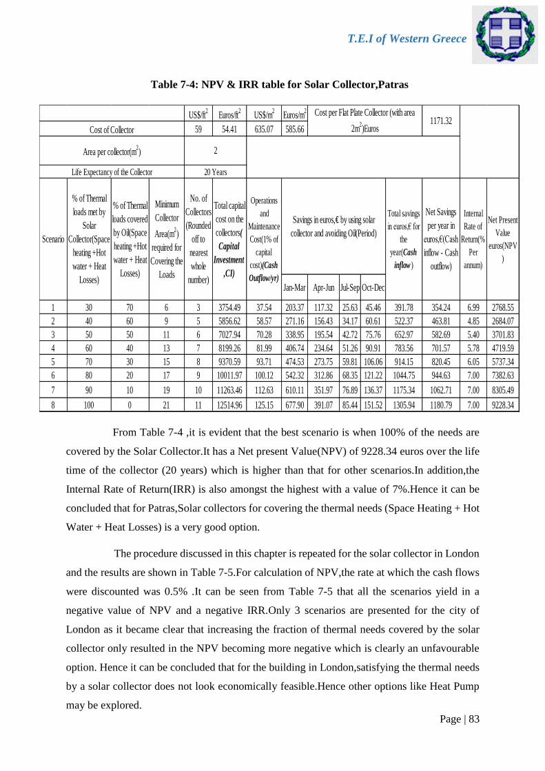
T.E.I of Western Greece
Page | 83
US$/ft2
Euros/ft2
US$/m2
Euros/m2
59 54.41 635.07 585.66
Jan-Mar Apr-Jun Jul-Sep Oct-Dec
1 30 70 6 3 3754.49 37.54 203.37 117.32 25.63 45.46 391.78 354.24 6.99 2768.55
2 40 60 9 5 5856.62 58.57 271.16 156.43 34.17 60.61 522.37 463.81 4.85 2684.07
3 50 50 11 6 7027.94 70.28 338.95 195.54 42.72 75.76 652.97 582.69 5.40 3701.83
4 60 40 13 7 8199.26 81.99 406.74 234.64 51.26 90.91 783.56 701.57 5.78 4719.59
5 70 30 15 8 9370.59 93.71 474.53 273.75 59.81 106.06 914.15 820.45 6.05 5737.34
6 80 20 17 9 10011.97 100.12 542.32 312.86 68.35 121.22 1044.75 944.63 7.00 7382.63
7 90 10 19 10 11263.46 112.63 610.11 351.97 76.89 136.37 1175.34 1062.71 7.00 8305.49
8 100 0 21 11 12514.96 125.15 677.90 391.07 85.44 151.52 1305.94 1180.79 7.00 9228.34
Scenario
% of Thermal
loads met by
Solar
Collector(Space
heating +Hot
water + Heat
Losses)
% of Thermal
loads covered
by Oil(Space
heating +Hot
water + Heat
Losses)
Savings in euros,€ by using solar
collector and avoiding Oil(Period)
Operations
and
Maintenance
Cost(1% of
capital
cost)(Cash
Outflow/yr)
2
20 Years
Minimum
Collector
Area(m2)
required for
Covering the
Loads
No. of
Collectors
(Rounded
off to
nearest
whole
number)
Total capital
cost on the
collectors(
Capital
Investment
,CI)
Cost of Collector
Net Present
Value
euros(NPV
)
Cost per Flat Plate Collector (with area
2m2)Euros
1171.32
Area per collector(m2)
Life Expectancy of the Collector
Net Savings
per year in
euros,€(Cash
inflow - Cash
outflow)
Total savings
in euros,€ for
the
year(Cash
inflow )
Internal
Rate of
Return(%
Per
annum)
Table 7-4: NPV & IRR table for Solar Collector,Patras
Table 7-5: NPV & IRR table for Solar Collector, LondonTable 7-6: NPV & IRR table for Solar
Collector,Patras
From Table 7-4 ,it is evident that the best scenario is when 100% of the needs are
covered by the Solar Collector.It has a Net present Value(NPV) of 9228.34 euros over the life
time of the collector (20 years) which is higher than that for other scenarios.In addition,the
Internal Rate of Return(IRR) is also amongst the highest with a value of 7%.Hence it can be
concluded that for Patras,Solar collectors for covering the thermal needs (Space Heating + Hot
Water + Heat Losses) is a very good option.
The procedure discussed in this chapter is repeated for the solar collector in London
and the results are shown in Table 7-5.For calculation of NPV,the rate at which the cash flows
were discounted was 0.5% .It can be seen from Table 7-5 that all the scenarios yield in a
negative value of NPV and a negative IRR.Only 3 scenarios are presented for the city of
London as it became clear that increasing the fraction of thermal needs covered by the solar
collector only resulted in the NPV becoming more negative which is clearly an unfavourable
option. Hence it can be concluded that for the building in London,satisfying the thermal needs
by a solar collector does not look economically feasible.Hence other options like Heat Pump
may be explored.

T.E.I of Western Greece
Page | 84
US$/ft2
Euros/ft2
US$/m2
Euros/m2
59 54.41 635.07 585.66
Jan-Mar Apr-Jun Jul-Sep Oct-Dec
1 20 80 23 12 14055.88 140.56 128.09 89.47 29.87 73.08 320.51 179.95 -10639.09
2 30 70 34 17 19808.20 198.08 192.14 134.21 44.81 109.62 480.77 282.69 -14440.7
3 40 60 45 23 26940.44 269.40 256.18 178.94 59.74 146.16 641.03 371.62 -19884.3
Operations
and
Maintenance
Cost(1% of
capital
cost)(Cash
Outflow/yr)
Savings in euros,€ by using solar
collector and avoiding Oil(Period)
Total savings in
euros,€ for the
year(Cash
inflow )
Net Savings
per year in
euros,€(Cash
inflow - Cash
outflow)
Life Expectancy of the Collector 20 Years
Scenario
% of Thermal
loads met by
Solar
Collector(Space
heating +Hot
water + Heat
Losses)
% of Thermal
loads
covered by
Oil(Space
heating +Hot
water + Heat
Losses)
Minimum
Collector
Area(m2)
required for
Covering
the Loads
No. of
Collectors
(Rounded
off to
nearest
whole
number)
Total capital
cost on the
collectors(
Capital
Investment
,CI)
(negative)
Cost per Flat Plate Collector (with area
2m2)Euros
1171.32Cost of Collector
Area per collector(m2)
Internal
Rate of
Return(%
Per
annum)
Net Present
Value(NPV
)
2
Table 7-7: NPV & IRR table for Solar Collector, London
Table 7-8: NPV & IRR table for Solar Collector, London

T.E.I of Western Greece
Page | 85
RESULTS AND DISCUSSIONS
8.1 Comparison of Space Heating Load between the 2 approaches
The procedure explained in section 5.4.2 (Space Heating Load calculation by using
hourly temperature data) is repeated for the other seasonal months of London , continued for
Patras and the results are tabulated and compared with the space Heating Loads calculated in
section 5.4.1 using the average monthly ambient temperature .
Table 8-1: Space heating Load using 2 approaches (comparison)
S.NO Approach Load London Patras
Jan Apr Jul Oct Jan Apr Jul Oct
1
Monthly
Ambient
Temperature
from
RetScreen Heating
(kWh)
4396.7 3284.9 1045.9 2535.4 3053.6 1837.2 0 858.317
2
Hourly
Temperature
data + 3 days
representative
day
4180.5 4013.3 1083.9 2786.4 2470.6 1626.5 0 555.3
As noticed from Table 8-1,the space heating loads calculated from both the approaches
match more or less with considerable difference in April for London and in January for Patras
(greater than 500 kwh in both cases) .
In April for London, the space Heating load calculated from the second approach is
much higher than that of the first approach.This is because the hourly temperature values(Refer
Table III-A, Appendix III for hourly values) on the 7 days considered is lower than the monthly
ambient temperature for April (9.5oC) as used in the first approach.This explains why the space
Heating load is higher in the second approach .The exact opposite case exists for Patras in
January i.e., the hourly temperature values exceed the monthly ambient temperature(10oC) in
many hours(Refer Table III-B ,Appendix III for hourly values) .
Hence coming to the question of which approach to adopt during calculation of space
Heating Load in general,the second approach (i.e., calculated using hourly values of ambient

T.E.I of Western Greece
Page | 86
temperature + 3 days representative day )takes preference over the other approach because the
hourly values represent a more accurate picture although the second approach is more time
consuming and extensive .However ,it is to be mentioned that in this thesis, the values
calculated using the first approach has been adopted .
8.2 Comparison of the sizing of stand-alone PV between the 2
approaches
The simulation approach described in section 6.4 is repeated for the other cities(Patras and
Chennai) and the results obtained are tabulated and compared with the results of the approach
in section 6.3 henceforth described as classical .
Table 8-2:Comparison of PV sizing details - Classic and Stochastic approaches
S.No Approach
London Patras Chennai
Peak
Power of
PV,Pm
(kW)
Corrected
Battery
Capacity,CL
(Ah)
Peak
Power of
PV,Pm
(kW)
Battery
Capacity,
CL(Ah)
Peak
Power of
PV,Pm
(kW)
Battery
Capacity,CL
(Ah)
1 Classic 8.8 2400 3.8 1000 2.19 600
2 Stochastic 4.11 940.59 1.95 451.57 1.27 372.38
% Decrease
in capacity
over classic
approach
-53.29 -60.81 -48.68 -54.84 -42.01 -37.94
As seen from Table 8-2,the stochastic approach results in much lower PV peak power
and installed Battery capacity compared to the classical approach which tends to oversize the
system depending on the autonomy factor.The percentage decrease in the installed peak power
of the PV is more than 40% for all the cities which can lead to substantial savings in
money.There is also a considerable decrease in the battery capacity which in turn means less
money invested in the case of the stochastic approach compared to the classical approach.
Hence for sizing of stand-alone PV systems ,the stochastic approach although involving
extensive and voluminous analysis (data comprising each hour for an entire month) is much
better as it leads to reduction in the Peak power,Pm of the PV and the Battery Capacity ,CL by
a considerable percentage with the loss of load probability(LLP) still under the 5% margin.

T.E.I of Western Greece
Page | 87
CONCLUSIONS
In order to convert an existing building into a Zero Energy Building, it is important to
reduce the energy demand of the building to a minimal before using Renewables.This is
achieved by the use of passive solar techniques wherein by means of the incoming solar
radiation through the windows the load of space Heating is reduced.
A single storey Building was considered in 3 cities .In order to convert the building into
a ZEB, the overall thermal Heat Losses coefficient for the building (UA)b was
calculated initially.This value can be suitably reduced (if it does not pertain to the
region’s local building regulations)by the use of proper insulation.
The building loads comprising Thermal (Space Heating + Domestic Hot Water + Heat
Losses) and the Electric loads was determined in each of the cities for the seasonal
months. The thermal energy demand for the building (Space Heating in London and
Patras) was reduced by factoring the Solar Gain through the Windows.Also a
comparison was made between the 2 approaches used to calculate Space Heating Load
and the 2 approaches used for sizing of stand-alone PV with discussion on the better
approach for each case.
A solar collector was selected to satisfy the thermal loads (Heating for London &
Patras) and for Chennai a Heat Pump was choosen to meet the cooling Load.It was
observed that 100% of the needs can be covered by Solar Collector in Patras with very
good Net Present Value(NPV) and Internal rate of Return(IRR).However, in London
the outcome with Solar Collectors was not so good and the thermal needs can be
satisfied by other means such as a Heat Pump.

T.E.I of Western Greece
Page | 88
APPENDICES
Appendix – I
Table I-A : Global(G) and Diffuse Solar Radiation(Gd) in W/m2 on representative day of
Seasonal months for Chennai
(Source : PVGIS CM-SAF)
Local
Solar
Time
Jan Apr July Oct
G Gd G Gd G Gd G Gd
06:07 - - 46 38 74 65 - - 06:22 - - 87 60 111 91 - - 06:37 58 46 136 80 150 115 80 64
06:52 101 66 189 98 191 136 120 86
07:07 149 85 244 114 231 156 163 106
07:22 200 102 301 129 270 174 206 125
07:37 251 117 358 142 309 190 249 141
07:52 303 131 414 153 346 204 292 156
08:07 353 142 469 163 381 216 333 168
08:22 402 153 522 171 415 227 372 179
08:37 448 162 573 178 446 236 409 188
08:52 492 169 621 183 475 243 444 196
09:07 533 175 666 188 502 249 477 202
09:22 572 181 708 191 527 254 507 207
09:37 607 185 747 194 550 258 534 212
09:52 639 188 782 195 570 261 559 215
10:07 667 191 813 197 587 263 581 217
10:22 692 192 841 197 603 264 600 219
10:37 714 194 865 198 616 265 617 220
10:52 732 195 885 198 627 266 630 221
11:07 747 196 901 198 635 266 641 221
11:22 757 196 913 198 642 267 649 222
11:37 765 196 921 198 646 267 655 222
11:52 768 197 925 198 648 267 657 222
12:07 768 197 925 198 648 267 657 222
12:22 765 196 921 198 646 267 655 222
12:37 757 196 913 198 642 267 649 222
12:52 747 196 901 198 635 266 641 221
13:07 732 195 885 198 627 266 630 221
13:22 714 194 865 198 616 265 617 220
13:37 692 192 841 197 603 264 600 219
13:52 667 191 813 197 587 263 581 217

T.E.I of Western Greece
Page | 89
14:07 639 188 782 195 570 261 559 215
14:22 607 185 747 194 550 258 534 212
14:37 572 181 708 191 527 254 507 207
14:52 533 175 666 188 502 249 477 202
15:07 492 169 621 183 475 243 444 196
15:22 448 162 573 178 446 236 409 188
15:37 402 153 522 171 415 227 372 179
15:52 353 142 469 163 381 216 333 168
16:07 303 131 414 153 346 204 292 156
16:22 251 117 358 142 309 190 249 141
16:37 200 102 301 129 270 174 206 125
16:52 149 85 244 114 231 156 163 106
17:07 101 66 189 98 191 136 120 86
17:22 58 46 136 80 150 115 80 64
17:37 24 24 87 60 111 91 44 40
17:52 - - 46 38 74 65 - - 18:07 - - 15 15 40 38 - -
Table I - B :Global(G) and Diffuse Solar Radiation(Gd) in W/m2 on representative day of
Seasonal months for London
(Source : Climate -SAF PVGIS)
Local
Solar
Time
Jan Apr July Oct
G Gd G Gd G Gd G Gd
04:22 - - - - 30 30 - -
04:37 - - - - 49 46 - -
04:52 - - - - 69 61 - -
05:07 - - - - 91 76 - -
05:22 - - - - 114 91 - -
05:37 - - 50 45 138 106 - -
05:52 - - 73 60 163 119 - -
06:07 - - 97 74 188 133 - -
06:22 - - 122 88 214 145 - -
06:37 - - 149 101 239 157 - -
06:52 - - 175 113 264 168 - -
07:07 - - 202 125 289 178 39 36
07:22 - - 228 135 314 187 57 49
07:37 - - 254 145 337 196 76 61
07:52 - - 279 154 360 204 95 72
08:07 - - 303 162 382 211 115 82
08:22 35 32 326 169 403 217 134 92

T.E.I of Western Greece
Page | 90
08:37 46 39 348 175 422 222 152 101
08:52 57 46 369 181 441 227 170 109
09:07 68 52 388 186 458 231 186 116
09:22 78 58 406 190 474 235 202 122
09:37 88 63 422 193 489 238 216 127
09:52 96 67 437 196 502 241 229 132
10:07 104 71 451 199 514 243 241 137
10:22 111 74 462 201 524 245 251 140
10:37 117 77 472 203 533 246 260 143
10:52 123 80 481 204 540 247 268 146
11:07 127 82 487 205 546 248 274 148
11:22 130 83 492 206 550 249 278 149
11:37 132 84 496 207 553 249 281 150
11:52 133 84 497 207 555 249 283 150
12:07 133 84 497 207 555 249 283 150
12:22 132 84 496 207 553 249 281 150
12:37 130 83 492 206 550 249 278 149
12:52 127 82 487 205 546 248 274 148
13:07 123 80 481 204 540 247 268 146
13:22 117 77 472 203 533 246 260 143
13:37 111 74 462 201 524 245 251 140
13:52 104 71 451 199 514 243 241 137
14:07 96 67 437 196 502 241 229 132
14:22 88 63 422 193 489 238 216 127
14:37 78 58 406 190 474 235 202 122
14:52 68 52 388 186 458 231 186 116
15:07 57 46 369 181 441 227 170 109
15:22 46 39 348 175 422 222 152 101
15:37 35 32 326 169 403 217 134 92
15:52 25 23 303 162 382 211 115 82
16:07 - - 279 154 360 204 95 72
16:22 - - 254 145 337 196 76 61
16:37 - - 228 135 314 187 57 49
16:52 - - 202 125 289 178 39 36
17:07 - - 175 113 264 168 22 22
17:22 - - 149 101 239 157 - -
17:37 - - 122 88 214 145 - -
17:52 - - 97 74 188 133 - -
18:07 - - 73 60 163 119 - -
18:22 - - 50 45 138 106 - -
18:37 - - 29 29 114 91 - -
18:52 - - - - 91 76 - -
19:07 - - - - 69 61 - -
19:22 - - - - 49 46 - -

T.E.I of Western Greece
Page | 91
19:37 - - - - 31 30 - -
19:52 - - - - 14 14 - -
Table I-C :Global(G) and Diffuse Solar Radiation(Gd) in W/m2 on representative day of
Seasonal months for Patras
(Source : Climate -SAF PVGIS)
Local
Solar
Time
Jan Apr July Oct
G Gd G Gd G Gd G Gd
05:07 - - - - 28 28 - - 05:22 - - - - 54 47 - - 05:37 - - - - 83 65 - - 05:52 - - 41 41 115 82 - - 06:07 - - 74 62 149 99 - - 06:22 - - 104 81 186 115 - - 06:37 - - 137 99 225 129 - - 06:52 - - 171 115 264 143 39 39
07:07 - - 206 131 304 156 57 57
07:22 - - 240 145 344 167 97 73
07:37 38 38 274 158 383 178 126 88
07:52 62 52 308 169 422 187 155 101
08:07 82 65 341 180 460 196 184 114
08:22 102 76 372 189 497 203 212 125
08:37 122 87 402 197 532 210 240 135
08:52 141 96 430 204 565 216 266 144
09:07 159 105 456 210 596 221 291 152
09:22 176 113 481 215 626 225 314 159
09:37 192 119 503 220 652 229 336 165
09:52 206 125 524 223 677 232 356 170
10:07 220 130 542 226 699 234 373 174
10:22 231 135 558 229 718 236 389 178
10:37 241 138 572 230 735 237 403 181
10:52 250 141 583 232 749 239 414 184
11:07 256 143 592 233 761 240 423 185
11:22 262 145 599 234 769 240 430 187
11:37 265 146 604 234 775 241 434 188
11:52 267 147 606 235 778 241 437 188
12:07 267 147 606 235 778 241 437 188
12:22 265 146 604 234 775 241 434 188
12:37 262 145 599 234 769 240 430 187
12:52 256 143 592 233 761 240 423 185
13:07 250 141 583 232 749 239 414 184

T.E.I of Western Greece
Page | 92
13:22 241 138 572 230 735 237 403 181
13:37 231 135 558 229 718 236 389 178
13:52 220 130 542 226 699 234 373 174
14:07 206 125 524 223 677 232 356 170
14:22 192 119 503 220 652 229 336 165
14:37 176 113 481 215 626 225 314 159
14:52 159 105 456 210 596 221 291 152
15:07 141 96 430 204 565 216 266 144
15:22 122 87 402 197 532 210 240 135
15:37 102 76 372 189 497 203 212 125
15:52 82 65 341 180 460 196 184 114
16:07 62 52 308 169 422 187 155 101
16:22 42 38 274 158 383 178 126 88
16:37 24 23 240 145 344 167 97 73
16:52 - - 206 131 304 156 70 57
17:07 - - 171 115 264 143 44 39
17:22 - - 137 99 225 129 22 21
17:37 - - 104 81 186 115 35 32
17:52 - - 74 62 149 99 19 19
18:07 - - 46 41 115 82 - - 18:22 - - 21 20 83 65 - - 18:37 - - 89 72 54 47 - - 18:52 - - 68 58 30 28 - -
19:07 - - 47 43 8 8 - -
T.E.I of Western Greece
Page | 93
Appendix – II
Table II – A : Monthly means of Irradiances ,Temperature and Humidity,Chennai
(Source : SoDa)
Table II – B : Monthly means of Irradiances ,Temperature and Humidity,London
(Source : SoDa)

T.E.I of Western Greece
Page | 94
Table II – C :Monthly means of Irradiances ,Temperature and Humidity,Patras
(Source : SoDa)

T.E.I of Western Greece
Page | 95
Appendix – III
Table III – A : Hourly Temperature values + 3 days representative day for London,April
(Source : Meteonorm)
Hour Ref
Temp(oC)
Hourly Temperature (oC)
12th day 13th day 14th day 15th day 16th day 17th day 18th day
1 22 8 6.4 4.8 4 4.3 2.7 4.4
2 22 8 5.6 4.5 3.7 4.2 2.7 4
3 22 7.5 5.3 4.8 3.8 4.2 2.6 4.3
4 22 7.1 5.3 4.4 3.5 4.3 2.7 4.6
5 22 7.2 4.9 4.6 3.6 3.8 2.5 4.8
6 22 7.7 4.9 5.1 3.2 5.1 3.7 5.8
7 22 8.1 5 5.1 4.4 5.4 4.1 6
8 22 9.2 5.5 5.2 5.4 5.8 4.7 6.9
9 22 9.8 6.2 4.8 5.4 6.3 5.6 8
10 22 10.5 7 4.6 6 7.4 6.6 8.6
11 22 11.4 7.4 4.5 6 8.3 7.5 9.6
12 22 12.2 7 5.5 6.6 9.3 8.2 10.7
13 22 12.8 6.8 5.9 7.3 10.4 9 12.2
14 22 12.9 6 6.1 7.4 10.7 8.8 12.2
15 22 12.9 6 6.3 7.6 10.9 9.1 11.7
16 22 12.4 6.2 6.4 7.7 10.7 9.5 11.9
17 22 12.3 6.3 6.2 8.2 9.7 9 11.7
18 22 10.8 6.3 6.3 7.2 8.6 8 10.4
19 22 10.5 5.7 5.3 7.3 6.8 8 9.9
20 22 9.4 6.3 5 6.5 5.7 7.7 8.9
21 22 8.8 6.8 5.1 5.4 5.5 6.4 8
22 22 7.7 5.9 4.6 4.9 4.6 5.3 7.3
23 22 6.4 5.4 4.6 4.6 3.8 5.6 6.3
24 22 6.8 4.6 4 4.4 2.4 5 6.4

T.E.I of Western Greece
Page | 96
Table III – B :Hourly Temperature values + 3 days representative day for Patras,January
(Source : Meteonorm)
Hour Ref
Temp(oC)
Hourly Temperature (oC)
14th day 15th day 16th day 17th day 18th day 19th day 20th day
1 22 8.5 11.2 14 11.9 10.1 10.4 11.7
2 22 8.5 12.2 14.5 11.7 10 10.3 11.2
3 22 8 11.8 14.2 12.1 9.8 10.9 11.2
4 22 8.3 11.1 15 12.2 9.2 11.1 11.9
5 22 8.6 11.1 14.5 11.8 8.8 11 11
6 22 8.8 12.1 13.8 11 8.6 10.6 10.7
7 22 8.6 12.4 14.1 11.4 8.5 9.8 10.9
8 22 9.4 13.1 14.6 11.4 8.2 10 11.3
9 22 9.5 13.7 15.3 10.7 8.5 10.6 11.5
10 22 9.2 13.9 15.2 11.3 9.2 11.1 11.3
11 22 9.6 13.8 15.5 11 9.9 11.7 11.8
12 22 10.1 14.9 15.9 10.1 10.7 13.3 12.1
13 22 10.6 14.6 17.5 9.6 12.2 14.2 13.1
14 22 11.3 15.3 19.4 9.8 13.1 15.4 13.7
15 22 11.8 14.8 19.9 10.9 13.9 16.7 14.9
16 22 11.7 14.5 20.4 11 13.9 16.7 15.5
17 22 12.3 14.7 19.5 10.5 13.2 16.6 15.8
18 22 11.8 14.9 18 10.4 12.9 14.7 14.4
19 22 12.1 14.7 16.5 10 11.8 14 12.8
20 22 12 14.6 15.4 10.4 11.5 13.4 12.2
21 22 12.2 14.1 14.3 9.8 11.9 12.2 12.3
22 22 11.6 13.8 13.3 10.3 11.7 11.6 11.4
23 22 12.1 14.3 12.8 10.5 10.8 11.8 10.9
24 22 12 14 12.6 9.9 10.6 12 11.3
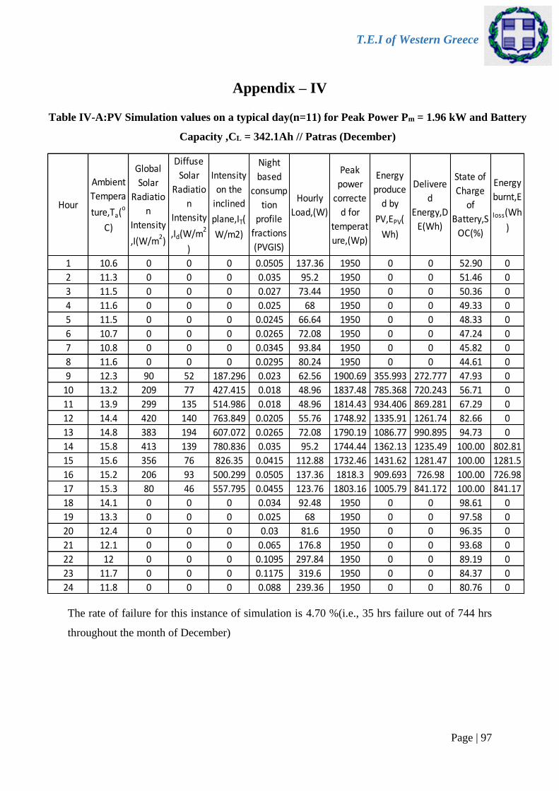
T.E.I of Western Greece
Page | 97
Hour
Ambient
Tempera
ture,Ta(o
C)
Global
Solar
Radiatio
n
Intensity
,I(W/m2)
Diffuse
Solar
Radiatio
n
Intensity
,Id(W/m2
)
Intensity
on the
inclined
plane,IT(
W/m2)
Night
based
consump
tion
profile
fractions
(PVGIS)
Hourly
Load,(W)
Peak
power
correcte
d for
temperat
ure,(Wp)
Energy
produce
d by
PV,EPV(
Wh)
Delivere
d
Energy,D
E(Wh)
State of
Charge
of
Battery,S
OC(%)
Energy
burnt,E
loss(Wh
)
1 10.6 0 0 0 0.0505 137.36 1950 0 0 52.90 0
2 11.3 0 0 0 0.035 95.2 1950 0 0 51.46 0
3 11.5 0 0 0 0.027 73.44 1950 0 0 50.36 0
4 11.6 0 0 0 0.025 68 1950 0 0 49.33 0
5 11.5 0 0 0 0.0245 66.64 1950 0 0 48.33 0
6 10.7 0 0 0 0.0265 72.08 1950 0 0 47.24 0
7 10.8 0 0 0 0.0345 93.84 1950 0 0 45.82 0
8 11.6 0 0 0 0.0295 80.24 1950 0 0 44.61 0
9 12.3 90 52 187.296 0.023 62.56 1900.69 355.993 272.777 47.93 0
10 13.2 209 77 427.415 0.018 48.96 1837.48 785.368 720.243 56.71 0
11 13.9 299 135 514.986 0.018 48.96 1814.43 934.406 869.281 67.29 0
12 14.4 420 140 763.849 0.0205 55.76 1748.92 1335.91 1261.74 82.66 0
13 14.8 383 194 607.072 0.0265 72.08 1790.19 1086.77 990.895 94.73 0
14 15.8 413 139 780.836 0.035 95.2 1744.44 1362.13 1235.49 100.00 802.81
15 15.6 356 76 826.35 0.0415 112.88 1732.46 1431.62 1281.47 100.00 1281.5
16 15.2 206 93 500.299 0.0505 137.36 1818.3 909.693 726.98 100.00 726.98
17 15.3 80 46 557.795 0.0455 123.76 1803.16 1005.79 841.172 100.00 841.17
18 14.1 0 0 0 0.034 92.48 1950 0 0 98.61 0
19 13.3 0 0 0 0.025 68 1950 0 0 97.58 0
20 12.4 0 0 0 0.03 81.6 1950 0 0 96.35 0
21 12.1 0 0 0 0.065 176.8 1950 0 0 93.68 0
22 12 0 0 0 0.1095 297.84 1950 0 0 89.19 0
23 11.7 0 0 0 0.1175 319.6 1950 0 0 84.37 0
24 11.8 0 0 0 0.088 239.36 1950 0 0 80.76 0
Table IV-A:PV Simulation values on a typical day(n=11) for Peak Power Pm = 1.96 kW and Battery
Capacity ,CL = 342.1Ah // Patras (December)
Table IV-A:PV Simulation values on a typical day(n=11) for Peak Power Pm = 1.96 kW and Battery
Capacity ,CL = 342.1Ah // Patras (December)
Appendix – IV
The rate of failure for this instance of simulation is 4.70 %(i.e., 35 hrs failure out of 744 hrs
throughout the month of December)

T.E.I of Western Greece
Page | 98
Hour
Ambien
t
Temper
ature,Ta
(oC)
Global
Solar
Radiation
Intensity,I
(W/m2)
Diffuse
Solar
Radiation
Intensity,
Id(W/m2)
Intensity
on the
inclined
plane,IT(
W/m2)
Night
based
consump
tion
profile
fractions
(PVGIS)
Hourly
Load,(W)
Peak
power
correcte
d for
temperat
ure,(Wp)
Energy
produce
d by
PV,EPV(
Wh)
Delivered
Energy,D
E(Wh)
State of
Charge
of
Battery,S
OC(%)
Energy
burnt,
Eloss(
Wh)
1 25.3 0 0 0 0.0505 186.345 1200 0 0 10.91 0
2 25.4 0 0 0 0.035 129.15 1200 0 0 8.58 0
3 25.3 0 0 0 0.027 99.63 1200 0 0 6.78 0
4 24.9 0 0 0 0.025 92.25 1200 0 0 5.11 0
5 24.7 0 0 0 0.0245 90.405 1200 0 0 3.48 0
6 24.8 0 0 0 0.0265 97.785 1200 0 0 1.71 0
7 24.6 26 26 25.557 0.0345 127.305 1195.86 30.56 -138.775 -0.31 0
8 25.1 73 73 71.756 0.0295 108.855 1188.38 85.27 -59.5224 -1.18 0
9 26.1 264 226 273.563 0.023 84.87 1155.68 316.15 203.26 1.78 0
10 27.9 567 308 631.242 0.018 66.42 1097.74 692.94 604.589 10.60 0
11 29.3 810 224 941.434 0.018 66.42 1047.49 986.14 897.79 23.70 0
12 29.6 729 384 796.844 0.0205 75.645 1070.91 853.35 752.729 34.68 0
13 30.6 440 375 447.626 0.0265 97.785 1127.48 504.69 374.621 40.15 0
14 31.6 503 376 525.906 0.035 129.15 1114.8 586.28 414.49 46.19 0
15 31.6 314 288 316.069 0.0415 153.135 1148.8 363.10 159.403 48.52 0
16 30.5 184 180 182.345 0.0505 186.345 1170.46 213.43 -34.4431 48.02 0
17 29.4 76 76 74.705 0.0455 167.895 1187.9 88.74 -134.587 46.05 0
18 28 10 10 9.830 0.034 125.46 1198.41 11.78 -155.103 43.79 0
19 27.5 0 0 0 0.025 92.25 1200 0 0 42.12 0
20 26 0 0 0 0.03 110.7 1200 0 0 40.12 0
21 26.6 0 0 0 0.065 239.85 1200 0 0 35.79 0
22 25.7 0 0 0 0.1095 404.055 1200 0 0 28.49 0
23 24.8 0 0 0 0.1175 433.575 1200 0 0 20.66 0
24 25.1 0 0 0 0.088 324.72 1200 0 0 14.79 0
Table IV-B: PV Simulation values on a typical day(n=15) for Peak Power Pm = 1.2 kW and
Battery Capacity ,CL = 285.6 Ah //Chennai (November)
Table IV-B: PV Simulation values on a typical day(n=15) for Peak Power Pm = 1.2 kW and
Battery Capacity ,CL = 285.6 Ah //Chennai (November)
The rate of failure for this instance of simulation is 13.75%(i.e., 99 hrs failure out of 720 hrs
throughout the month of November)

T.E.I of Western Greece
Page | 99
REFERENCES
[1] A. Ferrantea, M.T. Cascella. “Zero energy balance and zero on-site CO2 emission housing
development in the Mediterranean climate”. Energy and Buildings 43 (8) (2011) 2002–2010.
[2] A guide to Energy management in Buildings – Douglas J.Harris . Last Visit on Oct 28
,2015.http://www.btstor.cc/a-guide-to-energy-management-in-buildings-pdf-wd-
tf4275521.html.
[3] A.J. Marszal, P. Heiselberg, J.S. Bourrelle, E. Musall, K. Voss, I. Sartori , A. Napolitano.
“Zero Energy Building – A review of definitions and calculation methodologies”. Energy
Volume 54, 1 June 2013, Pages 1–10.
[4] Biomass Energy Centre.Last Visit on Dec 21,2015.
http://www.biomassenergycentre.org.uk/portal/page?_pageid=75,20041&_dad=portal.
[5] British Central Bank’s interest rate. http://www.global-rates.com/interest-rates/central-
banks/central-bank-england/boe-interest-rate.aspx.
[6] Chang, J. H. (1967), "The Indian Summer Monsoon", Geographical Review 57 (3): 373–
396.
[7] Danny H.W. Li , Liu Yang , Joseph C. Lam. “Zero energy buildings and sustainable
development implications - A review”. Energy 54 (2013) 1 -10.
[8] D. Kolokotsa , D. Rovas , E. Kosmatopoulos , K. Kalaitzakis. “A roadmap towards
intelligent net zero- and positive-energy buildings”. Solar Energy Volume 85, Issue 12,
December 2011, Pages 3067–3084.
[9] E. Kaplani , S. Kaplanis . “A stochastic simulation model for reliable PV system sizing
providing for solar radiation fluctuations” . Applied Energy 97 (2012) 970–981.
[10] EPBD recast, Directive 2010/31/EU of the European Parliament and of the Council of
19 May 2010 on the energy performance of buildings (recast), Official Journal of the European
Union, (2010) 18/06/2010.
[11] European Commission Energy Policy.Last Visit on Dec 17,2015 .
http://ec.europa.eu/energy/observatory/reports/latest_prices_with_taxes.pdf
http://www.global-rates.com/interest-rates/central-banks/central-bank-england/boe-interest-rate.aspx

T.E.I of Western Greece
Page | 100
[12] Frank Kreith / Jan F.Kreider . “ Principles of Solar Engineering” . Hemisphere Publishing
Corporation.67890 KPKP 8321.
[13] Hellenic Ministry of Environment Energy & Climate Change.Last Visit on Sep 3,2015.
http://www.ypeka.gr/Default.aspx?tabid=37&locale=en-US&language=el-GR.
[14] H. Lund , B. Moller , B.V. Mathiesen , A. Dyrelund. “The role of district heating in future
renewable energy systems”. Energy 35 (2010) 1381–1390.
[15] H. Lund , A. Marszal , P. Heiselberg . “Zero energy buildings and mismatch compensation
factors”. Energy and Buildings 43 (2011) 1646–1654.
[16] IEA HPP Annex 40.Last Visit on Aug 20,2015.
[17] Indian Green Building Council – Building Insulation Bulletin.April 2008.Last Visit on
Sep 17,2015. https://igbc.in/igbc/html_pdfs/technical/Building%20Insulation.pdf .
[18] J. Laustsen, Energy Efficiency Requirements in Building Codes, in: Energy Efficiency
Policies for New Buildings, OECD/IEA, Paris, 2008.
[19] Liping Wang, Julie Gwilliam, Phil Jones.” Case study of zero energy building design in
UK”. Energy and Buildings 41 (2009) 1215–1222.
[20] P.A. Torcellini, D.B. Crawley . “Understanding zero-energy buildings”. ASHRAE
Journal 48 (9) (2006) 62–69.
[21] The IEA SHC Task 40/ECBCS Annex 52 ‘Towards Net Zero Energy Solar Buildings
(NZEBs)’.
[22] US DOE, Building Technologies Program, Planned Program Activities for 2008–2012,
Department Of Energy, US. http://www1.eere.energy.gov/buildings/mypp.html , 2008
(downloaded 01/07/2010).
[23] Technical Chamber of Greece TEE.Last Visit on Sep 15 ,2015.
http://portal.tee.gr/portal/page/portal/TEE_HOME.
[24] 1993 ASHRAE Book of Fundamentals.
[25] Indian Standard Code of practice for construction of Brick-Cum-Concrete
Composite(Madras Terrace) Floor and Roof. Last Visit on Nov 12,2015.
https://law.resource.org/pub/in/bis/S03/is.2119.1980.pdf .

T.E.I of Western Greece
Page | 101
[26] K. Voss, A. Goetzberger, G. Bopp, A. Häberle, A. Heinzel, H. Lehmberg. “The
selfsufficient solar building in Freiburg—results of 3 years of operation” .Solar Energy 58 (1–
3) (2007) 17–23.
[27] NREL – National Renewable Energy Laboratory. Last Visit on Dec 19,2015.
http://www.nrel.gov/analysis/tech_lcoe_re_cost_est.html .
[28] S. Kaplanis & E. Kaplani. “Renewable Energy Systems: Theory, Innovation and
Intelligent Applications”. Nova Publisher, NY, 2013. ISBN 978-1-62417-741-5 .
[29] US Department of Energy . Solar Decathlon 2009. Integrated Design –Delivery and
Operations of Net-Zero Energy Buildings .
[30] Liping Wang, Julie Gwilliam, Phil Jones. “Case study of zero energy building design in
UK”. Energy and Buildings 41 (2009) 1215–1222 .
.