A Method to Justify Process Control Systems in Mineral ...

Iran. J. Chem. Chem. Eng. Vol. 32, No. 4, 2013

105��

A Method to Justify Process Control Systems in

Mineral Processing Applications

Parsapour, Gholamabbas

Mining Engineering Goup, Shahid Bahonar University of Kerman, P.O. Box 76175-133 Kerman, I.R. IRAN

Maleki, Mostafa

Mining Engineering Group, ValiAsr University of Rafsanjan, P.O. Box 518 Rafsanjan, I.R. IRAN

Banisi, Samad*+

Mining Engineering Goup, Shahid Bahonar University of Kerman, P.O. Box 76175-133 Kerman, I.R. IRAN

ABSTRACT: The impact of installing process control systems can be expected in terms of

performance improvements through reduced operating costs. Since these installations impose

considerable capital expenditure, the profitability of the new systems should be economically

justified. Controlled variable trend was reconstructed by a combination of simple waves, which

provided a means to simulate the effect of installing a control system (feedback) by removing

disturbance waves with high periods (> one cycle per hour). A method was proposed to evaluate

the impact of installing a control system either by a reduction of difference between concentrate

target quality and operating quality (i.e., bias reduction) or by reduction of scatter of product

quality (i.e., variance reduction). Installing automatic control systems not only reduces operating

costs, but also may increase revenue from washed coal sales by maintaining plant performance

on designed or desired target. It was found that if an appropriate feedback control system is used

at the flotation circuit of the Zarand coal washing plant, the variance of concentrate ash content could be

decreased from the current value of 0.38 to 0.06. Based on the predicted metallurgical

improvement, the payback time of installing a conventional control system for the flotation circuit

of the Zarand plant size with the approximate cost of $1,000,000 was found to be 2 years.

KEY WORDS: Control system, Justification, Zarand coal washing plant.

INTRODUCTION

Process control has become widely recognized as

an essential component of any processing operation [1-3].

It has direct impact on productivity, process efficiency

and product marketability. The reported paybacks

associated with successful installations underscore this

observation. As a consequence, many operators who

have not utilized process automation are looking to initiate

control projects, while those who currently use some

level of automation are looking to upgrade existing

control systems [4].

* To whom correspondence should be addressed.

+ E-mail: [email protected]

1021-9986/13/4/105 11/$/3.10

Iran. J. Chem. Chem. Eng. Parsapour Gh. et al. Vol. 32, No. 4, 2013

��

106

Important advances have been made in the field of

automatic control of mineral processing operations,

particularly in grinding and flotation. The main reasons

for this rapid development are [5]:

- The development of reliable instrumentation for

process control systems. On-line sensors such as

flowmeters, density gauges, chemical composition

analyzers, and on-line particle size analyzers have been

successfully used in many plants [6].

- The availability of sophisticated digital computers

at very low cost. The development of the microprocessor

allowed very powerful computer hardware to be housed

in increasingly smaller units. The development of

high-level languages allowed relatively easy access

to software, providing a more flexible approach to changes

in control strategy within a particular circuit.

- A more thorough knowledge of process behavior,

which has led to more reliable mathematical models of

various important unit processes being developed [7].

Often the improved knowledge of the process gained

during the development of the model has led to improved

techniques for the control of the system.

- The increasing use of very large grinding mills and

flotation cells has facilitated control, and reduced

the amount of instrumentation required.

Financial models have been developed for the

calculation of costs and benefits of the installation of

automatic control systems [8-12], and benefits reported

include significant energy savings, increased

metallurgical efficiency and throughput, and decreased

consumption of reagents, as well as increased process

stability [13-16].

The question most frequently asked is: "What will

automation cost and what will the economic benefits be?"

To answer this question a complete justification study

is needed. If the project team has little related experience

providing a good answer is challenging. In most cases

the costs, benefits and time requirements are

underestimated. Project cost and time requirements tend

to be somewhat easier to define, once the project scope

is properly defined. Benefits present a more difficult

problem since they require the impact of control system

on the process [4].

The purpose of this paper is to describe and demonstrate

a method which can be applied to estimate these potential

benefits, for certain types of control objectives.

The method is based on characterisation of the controlled

variable fluctuation and the effect of control system

on reducing the variation. The justification problem

will be introduced in general terms, and the underlying

theory then will be explained along with a practical

example from a coal processing plant in Kerman area.

The justification problem: A background

A process control system can impose significant

capital and operating costs on process economics.

For example, a retrofit control system project on an

operation with predominantly manual controls can incur

capital costs in excess of one million dollars. A great deal

of instrumentation, hardware and software must be

purchased/developed, installed and maintained.

Management must be convinced that the project has

a high probability of meeting its stated improvement goals

with an acceptable financial return. In completing

a justification study, one must consider all of the costs and

benefits of the proposed project to ensure that

management's interests are well satisfied [10].

The control system justification study can be thought

of as a three step process:

- Identify and prioritize the potential control

applications in the plant. Choose the application with

the greatest potential.

- Evaluate the technical merit of the proposed control

system.

- Evaluate the economic impact of the proposed

control system.

Although there can be many reasons for investigating

process control, e.g. environmental, safety, etc., better

economic performance is the principal driving force

to look for improvements in this area.

Usually the project costs are relatively easy to estimate

based upon supplier data and information available from

consultants. The benefits are more difficult to deal with.

In this paper the focus is on the evaluation of the benefits

of process control and, in particular, on the notion of increasing

operating efficiency by operating at target values for

the major production variables, while minimizing the variations

that occur due to disturbances. Although cost reductions can

be significant and will sometimes be enough to justify

a control project, operating efficiency generally provides

for much larger returns [4].

Iran. J. Chem. Chem. Eng. A Method to Justify Process Control Systems ... Vol. 32, No. 4, 2013

��

107

The technical and the economic merit of a proposed

control system application are very important.

The technical merit is assessed using the signal variance

spectrum and the economic merit is estimated using

the results of improvement in the technical evaluation.

There are several methods to evaluate the benefits

of process control. In the order of increasing cost and

increasing confidence in the results, these are:

- analysis of historical data

- plant studies

- dynamic simulation studies

- prototype control system testing on a portion of the plant

Plant studies may include some of the elements of

the analysis of historical data as well as some of the sampling

work that would be associated with dynamic simulation.

The method to be described falls into the second

category. It is similar in concept to the dynamic

simulation approach although approximations are

employed to characterize disturbances. In addition,

the analysis is conducted in the frequency domain and not

the time domain usually associated with dynamic simulation.

THEORETICAL SECTION

Characterizing Disturbances

Process disturbances can be characterized by source

and pattern. It is sometimes necessary to identify

the potential sources of disturbances by careful consideration

of the process inputs and operating features. In the

method described in this paper the disturbances

are lumped into a single, undefined source. With regard

to pattern, in most process control applications various

theoretical disturbance patterns, e.g. step change, ramp

change and sinusoidal change are considered. In the

proposed approach of justification, process disturbances

are assumed to follow sinusoidal patterns.

Under the assumption that the process is linear,

sinusoidal disturbances will be reflected as sinusoidal

variations in the controlled variable. In practice the

characterization is accomplished by high frequency

sampling of the controlled variable. A Fourier series

is then fitted to the time series which allows for the

transformation of the data in the time domain to

a variance spectrum in the frequency domain [11].

One source of experimental error which is not always

mentioned is that which derives from the measurements,

e.g. sampling, preparation and analytical errors.

This error could introduce a bias in the variance spectrum.

It is important that in all sampling campaigns to take every

effort to minimize the measurement error [4].

Typically, manual control is associated with low

frequency-wide range fluctuations on the controlled

variable. It is an experimental fact that, for many kinds of

waves, two or more waves can traverse the same space

independently of one another.

The importance of the superposition principle

physically is that it makes it possible to analyze a

complicated wave motion a combination of simple

waves. In fact it was shown by Fourier all that we need

to build the most general form of periodic wave are

simple harmonic waves. Fourier showed that any

periodic motion of a particle can be represented as

a combination of simple harmonic motions. The general

expression of such a combination is called a Fourier

series [17]:

�� (1)

where:

yi= predicted value of the controlled variable at time i

a0= average value of yi

k= wave number and kmax= last wave

Ak, �k= Fourier coefficients for frequency component

k (Ak = Amplitude and �k = Phase)

N= number of data points in the controlled variable

data record

If it is assumed that the disturbance affecting the

process is a sawtooth wave (Fig. 1), it could be reconstructed

by considering only first six terms of the Fourier series each

being a simple harmonic wave (Fig. 2).

The Fourier series for the above sawtooth wave

approximation is:

�� !� �� ! � � �"� �� " �#############�!� � �$� �� $ � � �%� �� % � � �&� �� & �

where � is angular frequency.

Determination of Fourier series coefficients

In order to produce simple harmonic waves their

amplitude (A) and phase (�) should be determined. Eq. (1)

could be expanded to obtain:

Iran. J. Chem. Chem. Eng.Iran. J. Chem. Chem. Eng.

108

'( � �� ######)* ��

��If

+,�� and

�� -then:

�� )��

�Eqs. 7 and

[18-19]:

� � !.��

��

Y (

t)

Y (

t)

Iran. J. Chem. Chem. Eng.

#########################� !�/�. �0,��

�#

##

)*� �� !��

�� and 8 have been proposed to calculate a

� 1� *!�/�. 2####

0.4

��

0.2

��

0

��

-0.2

��

-0.4

0.4

��

0.2

��

0

��

-0.2

��

-0.4


Fig.

##########################� �� 0,�

!�/�. � � - 0,� have been proposed to calculate a

2 #########################

-(1/ππππ) sin(ωωωωt)

-1/(4ππππ) sin(4ωωωω

Parsapour Gh. et al.

. 1: A disturbance represented by a sawtooth wave

Fig. 2: The First six terms of the series

#########################0,�� !�/�. �2

0,�� !�/�. �2####### have been proposed to calculate ak and b

#########################

t)

ωωωωt)


A disturbance represented by a sawtooth wave

The First six terms of the series

# �"�

(4)

(5)

�&� and bk

##�3�#

- �

#45bk are computed by Eqs

kmax

Variance spectrum

superposition of simple harmonic waves, the total

variance of the wave is summation of variance of each

simple wave. If the variance of each simple wave

is calculated then the variance spectrum could be obtaine

In this research, the variance spectrum was calculated

-1/(2ππππ) sin

-1/(5ππππ) sin

t


A disturbance represented by a sawtooth wave

The First six terms of the series.

� !.�� +,��

��Using Eqs. (4

� 6�� -�� 789:7; <=>=If N is an odd number then k

are computed by Eqs

max = N/2, ��Variance spectrum

When a disturbance wave is reconstructed by






sin(2ωωωωt)

sin(5ωωωωt)

t

A disturbance represented by a sawtooth wave.

+,� *!�/�. 2#########4) and (5) one could arrive at:

�############

If N is an odd number then k

are computed by Eqs. (7) and

�� ? ��

Variance spectrum







-1/(3

-1/(6

Vol. 32

#########################one could arrive at:

If N is an odd number then kmax =(N-1)/

and (8). If N is even number

�� and -��







3ππππ) sin(3ωωωωt)

6ππππ) sin(6ωωωωt)

32, No. 4, 2013

��

####################�@�one could arrive at:

(9)

(10)

)/2 and ak and

If N is even number

�� A.





is calculated then the variance spectrum could be obtained.


2013

��

�

)

)

and

If N is even number





d.



��

109

Table 1: Twelve samples (N=12) taken from a controlled variable with time intervals of 20 min.

3.4 4.5 4.3 8.7 13.3 13.8

16.1 15.5 14.1 8.9 7.4 3.6

Table 2: Fourier coefficients of six simple harmonic waves approximating the signal.

k ak

(Eq. 6) bk

(Eq. 7) Ak

(Eq. 8) B5� � CD5�! E fk=k/N pk= 1/fk pk/3 (h)*

1 -5.30 -3.81 6.53 21.30 0.08 12.00 4.00

2 0.05 0.17 0.18 0.02 0.17 6.00 2.00

3 0.10 0.50 0.51 0.13 0.25 4.00 1.33

4 -0.52 -0.52 0.74 0.27 0.33 3.00 1.00

5 0.08 -0.59 0.59 0.17 0.42 2.40 0.80

6 0.30 0.00 0.30 0.05 0.50 2.00 0.67

* Note that since every 20 minutes samples were taken then to convert the period to hours they were divided by 3.

Table 3: Variance contribution of waves with various periods.

Lower-upper limits on period (hours) Variance (mm2)

2-4 21.32 (21.30+0.02)

� � �F GH 0.40 (0.13+0.27)

AF&3 � AF GH 0.22 (0.17+0.05)

using data collected from sampling of the process. The

variance of each wave (�2k) was calculated by [4]:

I� � C�! E #####J,K#/ � �L !L M L /NOP#################################��

Each �k2 is a variance of a wave with a frequency of fk

(k/N) and a period of pk (1/fk.). Therefore, k number of

variances and periods are obtained. The total signal

variance would then be:

IQRSOT� � � I��

��##################################################################��!�

Variance spectrum calculation procedure

To illustrate the method it is assumed that 12 samples

(N=12) with the time intervals of 20 minutes are

collected from a controlled variable (Table 1). For N=12,

kmax=6 which means six waves could be superposed

to approximate the controlled variable behavior.

Then Fourier coefficients and variances were

calculated using Eqs. (6) to (8) as shown in Table 2.

The six waves could be grouped into three based

on the magnitude of their periods (Table 3). The grouping

is arbitrary and does not affect the final results.

The contribution of each group variance on the overall signal

variance could then be calculated by summing the

individual variances.

The variance spectrum of the signal (controlled

variable) which could be approximated by six harmonic

waves is shown in Fig. 3. The effect of installing a

control system could be evaluated by removing variance

contribution of the waves which could be eliminated

by the control system [20].

Modeling the effect of control system on the process

It is assumed that both disturbance dynamics and the

process control dynamics can be modeled as a simple first

order linear system because linear approximations are

often quite reasonable for control purposes. In these

systems a sinusoidal disturbance will present a sinusoidal

behavior in the process output. Feedback control system

which is often used in plants is most effective for low

frequency disturbance. In the high frequency, the process

acts as a filter and reduces amplitude ratio. The low


110

Fig. 3: Variance Spectrum of the controlled variable

frequency level has been found to be

most mineral and coal processing plants

Process control can remove disturbances with

frequencies lower than critical

hour). This translates to a reduction in the variance;

typically this variance reduction is substantial

QUANTIFING ECONOMIC IMPACT OF

VARIANCE REDUCTION

In most concentrate selling contracts either an average

quality (a*; target value) or a limit for off

(aL) products are defined. In other words, plants try

to produce a concentrate with a minimum variation from

the target value or try to reduce the amount of

off-specification products by reducing the dis

the concentrate quality values.

For further illustration, distributions of ash content

(undesirable elements) of

concentrate of the Zarand coal washing plant with and

without control system are shown in Fig

that using a control system will reduce the spread of

the concentrate ash content. The average ash contents (µ) and

standard deviations (

control are

respectively. This mean

off-specification products the target ash could be increased

which translates to a higher yield

limit of DMS concentrate ash (a

for no control case the amount of undesirable

(off-specification) could be

distribution curves characteristics (Z

25

��

��

20

��

15

��

10

��

5

��

0

Va

ria

nce

(m

m2)


Variance Spectrum of the controlled variable

frequency level has been found to be



frequencies lower than critical




VARIANCE REDUCTION


; target value) or a limit for off

) products are defined. In other words, plants try



specification products by reducing the dis



(undesirable elements) of D


without control system are shown in Fig



standard deviations (�) of concentrates without and with

control are 10.64%, 1.64%

respectively. This mean

specification products the target ash could be increased

which translates to a higher yield

limit of DMS concentrate ash (a


specification) could be

distribution curves characteristics (Z

2

Lower limit on


Variance Spectrum of the controlled variable

frequency level has been found to be 1 cycle per hour for



frequencies lower than critical frequency




VARIANCE REDUCTION


; target value) or a limit for off




specification products by reducing the dis



Dense Medium


without control system are shown in Fig.



) of concentrates without and with

1.64% and

respectively. This means that for the same amount


which translates to a higher yield (Fig. 4).

limit of DMS concentrate ash (aL) is assumed to be


specification) could be calculated using normal

distribution curves characteristics (Z-score):

1

Lower limit on period (h)


Variance Spectrum of the controlled variable.

cycle per hour for

most mineral and coal processing plants [10].


frequency (1 cycle per


typically this variance reduction is substantial, about 90%



; target value) or a limit for off-specification




specification products by reducing the distribution of


edium Separator (DMS)


. 4. It is assumed




and 10.92%, 0.99%

s that for the same amount


). If the acceptance

is assumed to be 11.5%

for no control case the amount of undesirable concentrate

calculated using normal

score):

0.67

period (h)


cycle per hour for


cycle per


90%.



specification




tribution of


eparator (DMS)


is assumed




0.99%,

s that for the same amount


If the acceptance

11.5%,

concentrate

calculated using normal

Fig.

a product at the Zarand coal washing plant.

U �

area to the left side of the distribution is equal to

which means

limit and is unacceptable to the buyer. If the use of the

control system results in a reduction of standard deviatio

from

area) then the new value of the target ash (µ

equal to

of the product could be increased.

Modeling relationship between quality and quantity of

products

a control system is to have a model to relate the quality

to the quantity of the products. Each point in

the relationship is a possible opera

evaluated economically. By using a control system the

operation moves to another location in this relationship

which could be justified if it has a superior economic

return over the no control case. It is then necessary

to estab

variables. Due to complexity, steady state models are

used instead of dynamic models. It has been found that

such approximation is appropriate when the disturbance

frequency is low

the product (ash content; a) and quantity (yield; y) relationship

was used to justify the use of a control system.

can be computed by:

Ash

dis

trib

uti

on


. 4: Impact of a control system on ash distribution of


� �V � WX ######YThe Z-score of


which means 28%



from 1.64 to 0.99%


equal to 10.92%.



products

A prerequisite to study the economic impact of








to establish the relationship between controlled and other




frequency is low



At the steady state average yield (

can be computed by:

6

0.45

0.40

0.35

0.30

0.25

0.20

0.15

0.10

0.05

0.00

Impact of a control system on ash distribution of


Y U � ��F% ��F$&score of 0.586 corresponds


28% of the concentrate in this case is out of



0.99%, (assuming the same unacceptable


. In practice,











lish the relationship between controlled and other




frequency is low [9]. In this study



At the steady state average yield (

can be computed by:

8 10

Ash (%)

Vol. 32



�AF&$$& � AF%@& corresponds to a point where the


of the concentrate in this case is out of



assuming the same unacceptable


, this means that the weight






the relationship is a possible operating case which should be









In this study, the quality of



At the steady state average yield (ZH) and ash (

12 14

Ash (%)

32, No. 4, 2013

��


%@&#############��"�to a point where the

area to the left side of the distribution is equal to 0.28



control system results in a reduction of standard deviation


area) then the new value of the target ash (µn) will be

this means that the weight





ting case which should be









he quality of


H) and ash (D[

14 16

2013

��


� to a point where the

0.28



n


) will be

this means that the weight





ting case which should be









he quality of


D[)


��

111

\] � ^ _��`�Q�^ _��`�Q�

###� ? _��a��? _�a�� ################################��$�#

] � ^ _��`�Q�^ _��`�Q�

� ? _��a��? _��a�� ########################��%� where

T: sampling period

F(t), Fi: solid feed rate at time t or i

y(t), yi: yield at time t or i

a(t), ai: concentrate ash content at time t or i

N: number of samples

One method to solve these integrations is to transform

time-dependent function (e.g., a(t)) to a probability

density function (e.g., p(a)):

b��`�� c b ��d��`��###################################��&�#�

ef

Q

�

Expanding y(a) about the desired operating point (y*, a*)

using Taylor series and ignoring terms with order three

and above:

�� g � h�� g� � i�� g�� (17)

where:

�g � ��g�############################################################################��@� h � �j��g� (19)

i � �jj��g�!k #########################################################################�!A� �j and �jj are first and second derivatives of y(a).

Substituting Eq. (17) in Eq. (14) and using probability

density functions properties and assuming constant feed

rate (i.e., F(t)=F) will give:

\] � ^ ��`�Q�^ `�Q�

� c^ ��d��`��#�efc^ d��`��#�ef�##################### �!��

b��g � h�� g� � i�� g��d��`��#�

ef

By integration and rearranging:

\] � �g � h��H � �g� � i��H � �g��lmmmmmmnmmmmmmopqqrsS

� iXO�tuOv�OS�Rw

###########�!!� where:

^ �d��`�� H########�ef ####################################################�!"� b�� H��d��`�� XO�################################################�!$��

ef

7H and x>� are the ash content average and variance,

respectively. Inspection of Eq. (22) indicates that

deviation of average yield (ZH) from the desired yield (y*)

could occur because of either low concentrate quality

(7H � 7g; offset) or high variation of concentrate ash

content (x>�; variation). Since � (second derivate) is

always negative any variation and offset will result

in deviation of the average yield from the desired yield.

The effect of poor control depends on the slope (�) and

curvature (�) of yield-ash curve at the desired operating

point (i.e., y*, a*). The use of a control system reduces

or eliminates the bias (7H � 7g); in other words#7H � 7g. Eq. (22) could be used to evaluate the effect of a control

system by comparing the average yield with and without

control. With no control case average yield will be lower

than desired yield because of offset and variation effects.

The difference between the yields of two cases should be

higher than the costs of the control system in order

to justify the use of control system.

Assuming a constant feed rate (F(t)=F) and

substituting Eq. (22) in Eq. (15), the weighted average

ash content could be calculated:

] � ^ ��`�Q�^ ��`�Q�

#� ######################################################## �!%� c^ ��g � h�� g� � i�� g��#d��`��#�e�c^ ��g � h�� g� � i�� g��d��`��#�e�

By proper integration and ignoring order three and

higher terms:

] � ######################################################################################## �!&� �g�H � h�XO� � �H� � �H�g� � i��H��H � �g�� XO��"�H � !�g��g � h��H � �g� � i��H � �g�� iXO�

Note that �H is the average of ash contents during

the sampling period (T) but ] is the weighted average of the

ash contents in which the mass of the concentrates are

also taken into consideration. The latter average is very

close to the real average. Eq. (26) provides the average

ash content with and without a control system through

the use of different values for � and �.


��

112

Table 4: Fourier coefficients and variances calculated for ash content trend line.

k ak bk Ak B� fk Pk Period (min) ?B�

1 0.0455 0.5386 0.5405 0.1461 0.0244 41.0 615.0 0.1906

2 -0.0239 0.2973 0.2982 0.0445 0.0488 20.5 307.5

3 -0.0080 0.2704 0.2705 0.0366 0.0732 13.7 205.0 0.0596

4 -0.1889 0.1021 0.2147 0.0230 0.0976 10.3 153.8

5 -0.1285 0.1724 0.2150 0.0231 0.1220 8.2 123.0 0.0360

6 0.0995 0.1257 0.1603 0.0129 0.1463 6.8 102.5

7 -0.0863 0.0791 0.1171 0.0069 0.1707 5.9 87.9 0.0087

8 0.0569 -0.0228 0.0613 0.0019 0.1951 5.1 76.9

9 -0.1000 0.1261 0.1610 0.0130 0.2195 4.6 68.3 0.0195

10 0.0538 0.1007 0.1142 0.0065 0.2439 4.1 61.5

11 -0.0775 -0.0531 0.0939 0.0044 0.2683 3.7 55.9 0.0082

12 0.0586 -0.0647 0.0873 0.0038 0.2927 3.4 51.3

13 -0.0882 -0.0665 0.1105 0.0061 0.3171 3.2 47.3 0.0141

14 -0.1265 0.0083 0.1268 0.0080 0.3415 2.9 43.9

15 -0.0876 -0.0727 0.1139 0.0065 0.3659 2.7 41.0 0.0102

16 -0.0741 -0.0451 0.0868 0.0038 0.3902 2.6 38.4

17 0.0180 0.0664 0.0688 0.0024 0.4146 2.4 36.2 0.0028

18 -0.0164 0.0253 0.0302 0.0005 0.4390 2.3 34.2

19 -0.1119 -0.1370 0.1769 0.0156 0.4634 2.2 32.4 0.0249

20 -0.1341 -0.0239 0.1362 0.0093 0.4878 2.1 30.8

EXPERIMENTAL SECTION

In order to use the proposed method, application of

a control system for the flotation circuit of the Zarand coal

washing plant was undertaken. Forty one samples of

flotation concentrate were taken with the time interval of

15 min and analyzed for ash content.

The concentrate ash content was used as the

controlled variable (yi) and Fourier coefficients along

with variances were calculated using Eqs. (6) to (10).

The variance spectrum was then obtained and

disturbances with the frequency lower than 1 cycle per

hour (periods larger than 1 hour) were removed

to simulate the effect of using a control system.

The removal process was carried out by assigning Ak=0

in Eq. (6). The controlled variable (concentrate ash

content; yi) was then predicted with the new coefficients

and average and standard deviation of predicated values

were calculated.

In order to obtain steady sate yield-ash curve

in a period of 3 months 9 sampling campaigns were

conducted and flotation circuit concentrate, tailing and

feed samples were analyzed for the ash content. The data

then was fitted with Eq. (17) to obtain � and �. The

average yield and ash were calculated using Eqs. (25)

and (26) for with and without control systems.

The predicated revenue when using the control system

was calculated considering the plant tonnage and

the coal market price.

RESULTS AND DISCUSSION

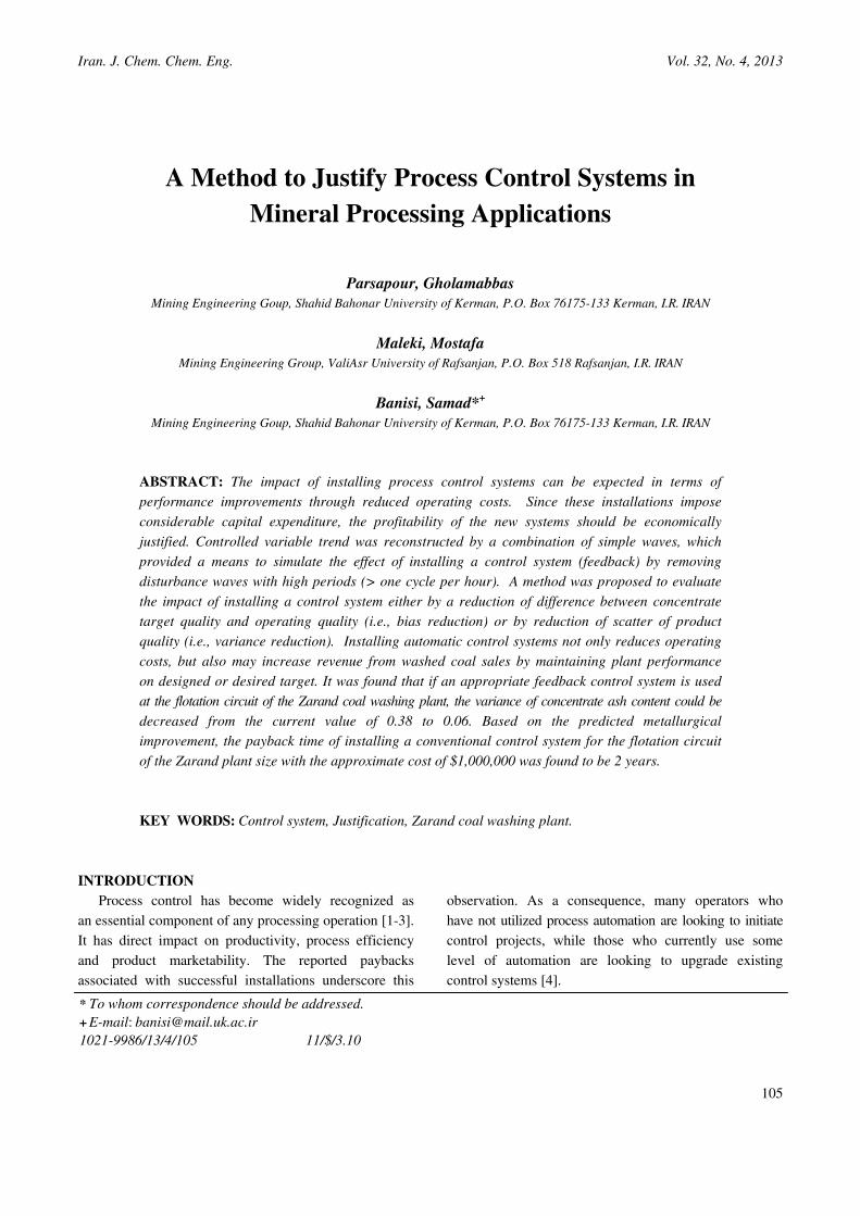
The results of sampling of concentrate over a period

of 615 minutes are shown in Fig. 5. The variation of the

concentrate ash content is rather high and has a

decreasing trend. The average ash content and variance

were calculated to be 10.17% and 0.38 (%)2, respectively.

Fourier coefficients and variance spectrum were

calculated using the procedure explained in theoretical

Section are shown in Table 4.

The variance contribution of various waves on the

overall trend line variance was calculated by grouping

waves based on their periods.

The variance contribution and the lower limit of the

period of each group were drawn in Fig. 6 which

is known as variance spectrum.


Fig. 5: Variation of ash content of flotation concentrate of

the Zarand coal washing plant.

Fig. 6: Variance spectrum of the concentrate ash content

trend line of the Zarand coal washing plant.

The highest variance contribution is associated with

disturbances with high periods. If the use of a control

system results in the removal of waves with periods of

more than one hour

will decrease from

reduction of 84%

In order to implement the removal of high period

disturbances from the signal (ash vs. time curve),

the coefficients of k from

Using the remaining coefficients, the ash content

was predicated over the sampling periods. The predicated

ash content trend which is the simulated behavior of

the system when the control system is used is shown in Fig

The average and variance of ash contents were obtained

to be 10.17 %

of ash content trends shown in Figs

lower variation when the control system is used.

11.5

11.0

10.5

10.0

9.5

9.0

8.5

8.0

Ash

(%

)

0

0.20

0.18

0.16

0.14

0.12

0.10

0.08

0.06

0.04

0.02

0.00��

Va

ria

nce

(%

)

308


Variation of ash content of flotation concentrate of


Variance spectrum of the concentrate ash content





more than one hour (~62

will decrease from 0.38 to

84%.



the coefficients of k from 1 to


predicated over the sampling periods. The predicated




% and 0.06 (%)

of ash content trends shown in Figs


100 200

308 154 103 77

Lower

Iran. J. Chem. Chem. Eng. A Method to Justify Process Control Systems








62 min), the overall variance

to 0.06 which indicates a relative



to 10 in Table






(%)2, respectively. Comparison

of ash content trends shown in Figs.


300 400

Time (min)

62 51 44

Lower limit on perion (min)

A Method to Justify Process Control Systems







the overall variance

ndicates a relative



in Table 4 was set to zero






espectively. Comparison

. 5 and 7 verifies


500 600 700

38 34 31

limit on perion (min)







the overall variance

ndicates a relative



was set to zero.




the system when the control system is used is shown in Fig. 7.


espectively. Comparison

verifies

Fig.

of the Zarand coal washing plant after using a control system.

Fig.

along with desired (target) operating point

taken along with desired (target) operating point and the

model fit is shown in Fig

to be

based on the operating and economic considerations. The

economic factors involved coal price, processing and

transportation costs

Eq. (

any give

��account only through the variance reduction (bias

reduction ignored), the yield with and without the control

system using Eq

respectively. Since the use of a contro

700

Ash

(%

) Y

ield

(%

)


. 7: Predicted variation of ash content of flotation concentrate


. 8: Steady state yield


The steady state yield


model fit is shown in Fig

The desired operating point of the plant was selected

to be 10.5% for ash content



transportation costs

. (27) which then used as the model to predict yield for

any given ash content.

�� &@ � %FGIf the effect of the control system is taken into

account only through the variance reduction (bias


system using Eq. (


11.5��

11.0

10.5

10.0

9.5

9.0

8.5

8.0��

Ash

(%

)

0 100

80

75

70

65

60

55

50��

9.0

A Method to Justify Process Control Systems ...

Predicted variation of ash content of flotation concentrate


Steady state yield-ash relationship for the samples taken


The steady state yield-ash relationship for the samples


model fit is shown in Fig. 8.


for ash content (



transportation costs. Fitting the data to Eq

which then used as the model to predict yield for

n ash content.

�� AF%� �If the effect of the control system is taken into



. (22) will be equal to


100 200 300

Time (min)

9.5 10.0

Vol. 32



ash relationship for the samples taken

along with desired (target) operating point and the model fit.

ash relationship for the samples



(a*) and 68% for yield



Fitting the data to Eq. (


� !FA�� AF%If the effect of the control system is taken into



will be equal to 65.98

respectively. Since the use of a control system is also

300 400 500

Time (min)

10.5 11.0

Ash (%)

Experimental data

Model

Target operation point

32, No. 4, 2013

��

113




and the model fit.




for yield (y*



. (17) provided


%��#############�!3�If the effect of the control system is taken into



65.98 and 66.62%

l system is also

500 600 700

11.5 12.0

Experimental data

Target operation point

2013

��

113






y*)



provided


� If the effect of the control system is taken into



66.62%,

l system is also


��

114

accompanied by a reduction in bias, which means that the

operating ash content becomes closer to the desired value,

the improvement in the efficiency of the process is more

than what is estimated here. The increase of 0.64%

in flotation circuit yield translates to yearly increase of

2560 t of concentrate. If the market price of coal is assumed

to be $250 per ton, the yearly revenue due to installing

a control system will be over $500,000. A conventional

control system for a flotation circuit of the Zarand plant

size with one controlled variable and four control loops

is about $1,000,000 which results in a payback time of

2 years.

CONCLUSIONS

- Controlled variable trend (i.e., concentrate ash content)

was reconstructed by a combination of simple waves, which

provided a means to simulate the effect of installing

a control system (feedback) by removing disturbance waves

with low frequency (> one cycle per hour).

- Metallurgical impact of installing a control system

in mineral processing applications was proposed to be

evaluated either by a reduction of difference between

concentrate target quality and operating quality (i.e., bias

reduction) or by reduction of scatter of product quality

(i.e., variance reduction).

- It was found that if an appropriate feedback control

system is used at the flotation circuit of the Zarand coal

washing plant, the variance of concentrate ash content

could decrease from the current value of 0.38 to 0.06.

- Based on predicted metallurgical improvement

installing a conventional control system for the flotation

circuit of the Zarand plant size with the approximate

cost of $1,000,000, the payback time was found to be

2 years.

Acknowledgements�

Mr. Haji-zadeh who performed all industrial sampling

and analysis with a great care deserves special appreciation.

The authors would like to thank Kerman Coal Mines

Company for supporting this research and permission

to publish this article. Special gratitude is also extended

to the operating, maintenance, metallurgy and R&D

personnel for their continued help.

Received : Oct. 3, 2011 ; Accepted : Aug. 26, 2013

REFERENCES

[1] Cipriano, A., Industrial Products for Advanced

Control of Mineral Processing Plants in “Advanced

Control and Supervision of Mineral Processing

Plants”, ed. Sbárbaro, D., and Villar, R. D.,

Springer, Chapter7, pp.287-308, (2010).

[2] Aldrich C., Marais C., Shean B.J., Cilliers J.J., Online

Monitoring and Control of Froth Flotation Ssystems

with Machine Vision: A Review, International

Journal of Mineral Processing, 96,p. 1 (2010).

[3] Bouche C., Brandt C., Broussaud A., Drunick V.W.,

Advanced Control of Gold Ore Grinding Plants in

South Africa, Minerals Engineering, 18, p. 866

(2005).

[4] Flintoff B.C., Neale A.J. , Hochstein R.F. , The

Justification of Process Control Systems in Mineral

and Coal Processing Applications, Proceedings,

22nd Annual Meeting of the CMP January16-18,

pp. 71-99, (1990).

[5] Wills, B. A. and Napier-Munn, T. J., “Will's Mineral

Pprocessing Technology”, 7th Edition, Elsevier

(2007).

[6] Edwards, R., Vien, A., and Perry, R., Strategies for

Instrumentation and Control of Grinding Circuits, in

“Mineral Processing Plant Design, Practice and

Control”, ed. A.L. Mular, D. Halbe, D.J. Barrett,

SME, pp. 2130-2151, (2002).

[7] King, R.P., “Modeling and Simulation of Mineral

Processing Systems”, Butterworth-Heinemann, 403

(2001).

[8] Purvis, J.R. and Erickson, I., Financial Models for

Justifying Computer Systems, INTECH (Nov.), 45.

(1982).

[9] Koenig R.L., Morrison R.D. and Simmons C.J., The

Selection and Financial Justification of Process

Control Instrumentation, Mill Operators'

Conference, North West Queensland Branch,

(1982).

[10] Neale, A.J., Flintoff, B.C., The Application of

Process Control in Canadian Coal Froth Flotation

Circuits, Advances in Coal and Mineral Processing

Using Flotation, Florida, Dec. 3-8, AIME, p.p. 289-

297, (1989).

[11] Dybeck M., Bozenhardt H., Justifying Automation

Projects, Chem. Eng., 20, p. 113 (1988).


��

115

[12] Garner K.C., Operability Studies or "Why Control",

Proc. Sem. On Measurement, Process Control and

Optimization in the Minerals Industry, SAIMM,

Paper NO.2, (1984).

[13] Koenig R.L., Morrison R.D, Simmons C.J., The

Selection and Financial Justification of Process

Control Instrumentation, Proc. Mill Operators

Conference, Australasian IMM, pp. 103-111, (1982).

[14] Barsamian J.A., Process Control Computer Systems:

Spend Money, Make Money, Intech, March, p. 31,

(1986).

[15] Latour P.R., The Hidden Benefits from Better

Process Control, Advances in Instrumentation,

31(1), ISA-76 Annual Conference, pp.528:1-11,

(1976).

[16] Shinskey F.G., The Values of Process Control, Oil &

Gas J., Feb. 18, pp. 80-83, (1974).

[17] Chatfield, C., “The Analysis of Time Series: An

Introduction”, 4th. ed., Chapman & Hall Press,

London, (1989).

[18] Kreysig, E., “Advanced Engineering Mathematics”,

5th. ed., New York: Wiley, (1983).

[19] Karal, Bury, "Statistical Distributions in

Engineering", Cambridge Univ. Press, Cambridge,

England, (1999).

[20] Sharifian M., Fanaei M. A., Dynamic Simulation

and Control of a Continuous Bioreactor Based on

Cell Population Balance Model, Iran. J. Chem.

Chem. Eng., 28(2), p. 15 (2009).

A Method to Justify Process Control Systems in Mineral ...

Documents

Transcript of A Method to Justify Process Control Systems in Mineral ...