A Matching-Related Property of BipartiteGraphs With Applications

in Signal Processing

Epameinondas Fritzilas a, Martin Milanic b, Jerome Monnot c

and Yasmin A. Rios-Solis d

a Faculty of Technology, Bielefeld University, Bielefeld, Germany

efritzil#cebitec.uni-bielefeld.de

b FAMNIT and PINT, University of Primorska, Koper, Slovenia

martin.milanic#upr.si

c LAMSADE, Universite Paris-Dauphine, Paris Cedex 16, France

monnot#lamsade.dauphine.fr

d Graduate Program of Systems Engineering, UANL, Monterey, Mexico

yasmin#yalma.fime.uanl.mx

Abstract

A bipartite graph G = (L,R;E) is said to be identifiable if for every vertex v ∈ L,the subgraph induced by its non-neighbors has a matching of cardinality |L| − 1.This definition arises in the context of low-rank matrix factorization. Motivated bysignal processing applications, in this paper we (i) propose the robustness of identi-fiability with respect to edge modifications as a polynomially computable measureof evaluating how strongly a bipartite graph possesses the property of identifiability,and (ii) introduce three problems that deal with finding identifiable subgraphs, andstudy their complexity.

Keywords: bipartite matching, complexity, combinatorial optimization,source-sensor network

1 Introduction

A matching in a graph is a subset of pairwise disjoint edges. A bipartitegraph G = (L, R; E) with at least one edge is called identifiable if for everyvertex in L, the subgraph induced by its anti-neighborhood has a matching ofcardinality |L| − 1.

As shown in [5], the concept of identifiable bipartite graphs arises naturallyin the context of low-rank matrix factorization, particularly in the area ofsignal processing: Suppose we have a set L of signal sources and a set Rof sensors, each measuring a linear mixture of the source signals over time.The exact values of the mixing coefficients are unknown. A bipartite graphG = (L, R; E) is given that specifies which sensors measure which sources;such a graph can often be inferred a priori, independently of the exact valuesof the mixing coefficients. Given the sensor measurements over k discrete timepoints, our task is to infer the source signals over the k time points and thenon-zero mixing coefficients. Formally, given an |R|×k matrix Y = (yit) whereyit is the signal measured at sensor i at time point t, we wish to express Y asa product Y = AX of an |R| × |L| matrix A = (aij), where aij is the mixingcoefficient between sensor i and signal source j, and a |L|×k matrix X = (xjt)that contains the source-signal intensities at different time points. Moreover,we require that the matrix A satisfies the constraints imposed by G (denotedby A ⊳ G), that is, (j, i) /∈ E implies aij = 0. We assume that |L| ≤min(|R|, k) (low-rank factorization). Since an exact low-rank factorization isimpossible in general, we seek a matrix pair (A, X) such that A ⊳ G and anappropriately chosen error measure ‖Y − AX‖ (e.g., the Frobenius norm) isminimized.

Now, let us suppose that we have obtained a feasible solution (A, X) to thisZero-Constrained Approximate Matrix Factorization (ZCAMF) problem. Many

other pairs (A, X) may exist that satisfy AX = AX and A ⊳ G, and are

therefore indistinguishable from (A, X) in terms of how well they approxi-

mate Y . However, the level set L = {(A, X) : AX = AX, A ⊳ G} of all suchpairs is in general restricted by the bipartite graph G. In particular, if G isidentifiable, and under some mild full-rank assumptions on the two factors Aand X, which are likely to be satisfied for numbers that correspond to physicalquantities 1 , the elements of the level set are unique up to diagonal scaling [5].That is, for every (A, X) ∈ L, there exists an invertible diagonal matrix D

1 Matrix X must have full row-rank and certain submatrices of A must have full column-ranks.

such that A = AD and X = D−1X.

Identifiable bipartite graphs will thus find applications in every area wherethe ZCAMF problem is relevant. In computational biology, for example, ZCAMFappears in at least two contexts: in determining the activities of transcriptionfactors from transcriptome data [9,3], and in microarray analysis [14].

Our Contributions

In the first part of the paper (Section 2), we define the robustness of identifiablebipartite graphs with respect to edge additions and deletions. This is usefulin applications where the sets of sensors and sources are known exactly, butthe structure of the bipartite network is predicted with some uncertainty (see,e.g., [9]). In practice, the robustness of bipartite graphs can be used as ameasure to select, among different sensor designs, the one that gives rise tothe “most identifiable” network. We show that robustness is computable inpolynomial time. In particular, we show that the robustness of a bipartitegraph G is equal to the minimum of the surpluses of certain subgraphs ofG, plus one. Based on two classical results on bipartite matchings, we givean efficient algorithm for computing the surplus of a general bipartite graph.Then, using the properties of the surplus function, we also develop a polytimealgorithm for computing a tight set.

In the second part of the paper (Section 3), we introduce and study severalvariants of the following problem: Given a bipartite graph G = (L, R; E), canwe delete some vertices D ⊂ L together with their neighbors so that theresulting graph is identifiable? This problem arises when the source-sensorgraph G is not identifiable, but we would still like to be able to measure asubset J = L\D of the signal sources in an “identifiable” way. If we omit thesources in D from our measurements, then we can use only the sensors thatdo not measure any source in D; this justifies why, together with each vertexin D, we must also delete all its neighbors. We identify several polynomiallysolvable cases, and show the hardness of the version of the problem in whichwe would like to keep as few vertices from L as possible so that the resultinggraph is identifiable. This latter problem arises in the context of ZCAMF whenthe number of time samples k is limited.

Notations and Definitions

All graphs considered are undirected, finite and loopless but may containparallel edges. To avoid trivialities, we only consider graphs with at least oneedge. For a graph G, we denote by V (G) the vertex set of G and by E(G)

its edge (multi)set. A bipartite graph is a triple (L, R; E) where (L ∪ R, E)is a graph such that E ⊆ L × R. Following the standard graph-theoreticterminology (see, e.g., [4]), we denote with ν(G) the matching number of agraph G, i.e., the maximum cardinality of a matching in G. For a graphG = (V, E) and a subset of vertices X ⊆ V , NG(X) denotes the neighborhoodof X, i.e., the set of all vertices in V \X that have a neighbor in X. For a vertexx ∈ V , we write NG(x) for NG({x}), and denote the degree of x with dG(x) =|NG(x)|. The anti-neighborhood of x ∈ V is the set V (G) \ (NG(x) ∪ {x}).In NG(X), NG(x), dG(x), we shall omit the subscript G if the graph is clearfrom the context. For a bipartite graph G = (L, R; E) and vertex sets X ⊆ L,Y ⊆ R, we denote by G[X, Y ] the subgraph of G induced by X∪Y . Moreover,for a vertex x ∈ L, we use Gx as a shortcut for G[L \ {x}, R \ N(x)]. Thesurplus of a set X ⊆ L is defined as σ(X) = |N(X)| − |X|. The surplus ofthe whole graph is defined as the minimum surplus over all non-empty sets:σ(G) = min∅6=X⊆L{σ(X)}. A set X ⊆ L is called tight if σ(X) = σ(G).

2 Robustness of Identifiable Graphs

In many applications (e.g., [9]), the sets of sensors and sources are known ex-actly, but the structure of the bipartite graph is predicted with some statisticalmethod. Such a prediction involves some uncertainty, i.e., some connectionsthat have been predicted as significant may not exist in reality and, viceversa, some existing connections may have been missed by the prediction. Inthis setting, a natural question arises: How many prediction mistakes can agiven bipartite graph tolerate, before it loses the property of identifiability?This quantity is defined below as the robustness of an identifiable graph. Inpractice, the robustness can be used in order to select among different sensordesigns the one that gives rise to the “most identifiable” network.

Definition 2.1 Let G = (L, R; E) be an identifiable graph. For a vertexx ∈ L, we define its robustness, denoted by ρ(x), as the minimum number ofedge modifications (additions and/or deletions) that are required to destroythe identifiability of x, i.e., to make ν(Gx) < |L| − 1. The robustness of thewhole graph is ρ(G) = minx∈L ρ(x).

Remark 2.2 The following construction shows that there exist graphs of ar-bitrarily high robustness: For two integers n > k ≥ 1, let Gn,k = (L, R; E) bethe graph given by L = {1, . . . , n}, R = {I ⊆ L : |I| = k} and (i, I) ∈ E iffi ∈ I. Using Proposition 2.3 below, it can be verified that ρ(Gn,k) =

(n−2

k−1

).

In the rest of this section, we prove that the robustness of a given identi-

fiable graph G, as well as a minimum-sized set of edge modifications requiredto destroy its identifiability, can be computed in polynomial time. First, weshow that computing the robustness reduces to computing the (non-negative)surpluses of the graphs Gx, for all x ∈ L.

Proposition 2.3 For every x ∈ L, ρ(x) = σ(Gx) + 1.

Proof. Consider a vertex x ∈ L. Adding (deleting) an edge incident to x,say (x, y), results in deleting (adding) the vertex y in Gx and this can onlydecrease (increase) ν(Gx). Adding (deleting) an edge (z, y), where z 6= x andy ∈ N(x), has no influence on Gx. Finally, adding (deleting) an edge (z, y),where z 6= x and y /∈ N(x), results in adding (deleting) the edge (z, y) in Gx

and this can only increase (decrease) ν(Gx). Therefore, in order to decreaseν(Gx), we must either add edges that are incident to x or delete edges thatare incident to some non-neighbor of x. Since both operations are allowedand have the same cost, we can safely focus only on edge additions, becausethey correspond to vertex deletions in Gx. More specifically, ρ(x) equals theminimum number of vertices that we must delete from R\N(x), such that thematching number of the remaining subgraph of Gx becomes less than |L| − 1.By Hall’s Marriage Theorem [6], this can only be achieved by choosing anonempty set Y ⊆ L \ {x} and deleting |NGx

(Y )| − |Y | + 1 vertices fromNGx

(Y ). Therefore, ρ(x) = min∅6=Y ⊆L\{x}{|NGx(Y )| − |Y |+ 1} = σ(Gx) + 1.

2

The above proof also shows that, in order to destroy the identifiability ofx ∈ L with a minimum number of edge modifications, it is enough to find atight set X in Gx and then add to G all the edges {(x, y) : y ∈ NGx

(X)}.

Motivated by the computation of robustness, in the following sections wepresent polynomial-time algorithms for computing the surplus and finding atight set in a bipartite graph G = (L, R; E). These results apply to arbitrarybipartite graphs and are interesting also outside the context of robustness,especially when the input graph G has σ(G) ≥ 0. In this case, G has an L-perfect matching and the following problem arises in any application that mustguarantee robust matchings: Find a minimum subset of R, whose deletionleaves G without L-perfect matching. For the solution it is enough to find atight set X ⊆ L and then delete an arbitrary set of σ(X) + 1 vertices fromthe neighborhood of X.

2.1 Computing the Surplus

Algorithm 1 below computes the surplus of a bipartite graph. Its correctnessis based on the following result (Theorems 1.3.1 and 1.3.6 in [10]).

Lemma 2.4 Let G = (L, R; E) be a bipartite graph. If σ(G) < 0, then σ(G) =ν(G)− |L|. If σ(G) ≥ 0, then σ(G) equals the largest integer s satisfying thefollowing property, for every x ∈ L: if we add s new vertices to L and connectthem to all neighbors of x, the resulting graph has non-negative surplus.

For the algorithm’s implementation we use a well-known theorem by Berge,a result of central importance for matching algorithms [1]. Berge’s theoremholds for arbitrary graphs and states that a matching M in a graph G ismaximum if and only if G has no M-augmenting path, i.e., a path whoseedges alternate between matched and unmatched and whose endpoints areunmatched. If there exists an M-augmenting path P , then a matching M ′

larger than M can be immediately obtained by replacing in M the matchededges along this path with the unmatched ones. In formulae, M ′ = M△E(P )where △ denotes the symmetric difference operator.

Algorithm 1 Computation of the surplus in G = (L, R; E)

1: Compute a maximum matching M in G.2: if |M | = |L| (i.e., σ(G) ≥ 0) then3: for all x ∈ L do4: sx ← 0, Mx ←M , Gx ← G5: repeat6: Gx ← (Gx with new vertex v∗ connected to all neighbors of x)7: if Gx has an Mx-augmenting path P then8: Mx ←Mx△E(P ) and sx ← sx + 19: else exit the repeat loop

10: end if11: end repeat12: end for13: σ(G)← minx∈L sx

14: else15: σ(G)← |M | − |L|16: end if17: return σ(G)

Proposition 2.5 Algorithm 1 computes the surplus of a bipartite graph G =(L, R; E). It can be implemented so that it runs in time O(|E|(

√|L|+ |R|+

|L|+ |E|)) (which is O(|E|2) if G has no isolated vertices).

Proof. By Hall’s Theorem, the augmented graph Gx (line 6) has non-negativesurplus if and only if there exists a matching that covers all vertices of Lx ∪{v∗}. By Berge’s Theorem this happens if and only if there exists an Mx-augmenting path (which has to start at v∗). Finally, the correctness of thealgorithm follows from Lemma 2.4.

It remains to analyze the running time. The computation of a maximummatching in line 1 can be done in O(|E|

√|L|+ |R|) time, using, e.g., the

algorithm of Hopcroft and Karp [7]. For each x ∈ L, the internal repeat-loopcan be executed up to d(x) times and, therefore, |E(Gx)| ≤ |E| + (d(x))2.In line 7, checking if Gx has an Mx-augmenting path and if yes, finding one,can be done as follows: First we orient all unmatched edges in Gx from L toR and all matched edges from R to L and then we look for a directed pathfrom v∗ to an unmatched vertex. This can be done with breadth-first searchin O(|E(Gx)|) time. In line 8, the symmetric difference can be computedin O(|E(Gx)|) time. So, the total running time is in O(|E|

√|L|+ |R| +∑

x∈L(|E|+ (d(x))2)) ⊆ O(|E|√|L|+ |R|+ |L||E|+ |E|2). The last inclusion

follows from:∑

x∈L(d(x))2 ≤(∑

x∈L d(x))2

= |E|2.

2

2.2 Finding a Tight Set

In this section, we show that we can find a tight set in G = (L, R; E) byusing an algorithm for surplus computation as a black-box routine in a greedyfashion (see Algorithm 2). For L′ ⊆ L, we denote with G − L′ the subgraphinduced by (L \ L′) ∪ R and we write G− x as a shortcut for G − {x}. Theneighborhood of any set X ⊆ L \ L′, is the same in G and in G − L′, and,therefore, for all X ⊆ L \ L′, σG−L′(X) = σG(X). So, we will omit theindex and write σ(X) := σG−L′(X) = σG(X). To prove the correctness ofAlgorithm 2 we need the following simple observations.

Proposition 2.6 Consider the graph G = (L, R; E) and a set L′ ⊂ L.

(i) σ(G− L′) ≥ σ(G)

(ii) If σ(G − L′) = σ(G), then, for all L′′ ⊆ L′, any tight set of G − L′′ isalso a tight set of G. In particular, it follows that σ(G− L′′) = σ(G).

(iii) Consider x ∈ L such that σ(G−x) = σ(G). Then, any tight set of G−xis a tight set of G.

(iv) σ(G−x) > σ(G) for all x ∈ L, if and only if L is the only tight set of G.

Proof.

(i) σ(G−L′) = minX⊆L\L′{σ(X)} ≥ minX⊆L{σ(X)} = σ(G). The inequalityfollows from the fact that we are minimizing the same objective functionover a larger ground set.

(ii) Let X∗ ⊆ L \ L′′ be a tight set of G − L′′. So, we have σ(X∗) =minX⊆L\L′′{σ(X)} ≤ minX⊆L\L′{σ(X)} = minX⊆L{σ(X)}. The inequal-ity follows from the fact that L \ L′′ ⊇ L \ L′ and the last equal-ity follows from the hypothesis σ(G − L′) = σ(G). So, we finally getσ(X∗) = minX⊆L{σ(X)}, i.e., X∗ is tight in G.

(iii) This is a special case of (ii) for L′′ = L′ = {x}.

(iv) Forward: For the sake of contradiction, assume that G has a tight setY ⊂ L. Then, Y is also tight in G−x, where x ∈ L\Y . That is, σ(Y ) =σ(G) = σ(G−x), which contradicts the hypothesis that σ(G−x) > σ(G).Reverse: For the sake of contradiction, assume that there exists x ∈ Lwith σ(G−x) = σ(G) (due to (i), it cannot be σ(G−x) < σ(G)). Then,there exists a set Y ⊆ L\ {x} that is tight in both G−x and G, and thiscontradicts the hypothesis that L is the only tight set.

2

Algorithm 2 below computes a tight set in the graph G = (L, R; E). Itstotal running time is of the order O(|L||E|(

√|L|+ |R| + |L| + |E|)), since

it requires |L| + 1 computations of surplus. Its correctness is established byTheorem 2.8.

Algorithm 2 Computation of a tight set in G = (L, R; E)

1: X ← L2: for all x ∈ L do3: if σ(G− x) = σ(G) then4: G← G− x and X ← X \ {x}5: end if6: end for7: return X

Lemma 2.7 Let H = (LH , RH ; E ′H) be a bipartite graph. Let v∗ ∈ LH such

that σ(H−v∗) > σ(H). If L′ = {v1, . . . , vi} ⊂ LH and σ(H−{v1, . . . , vj−1}) =σ(H − {v1, . . . , vj}) for all j = 1, . . . , i, then σ((H − L′)− v∗) > σ(H − L′).

Proof. Assume that the lemma fails. From assertion (i) of Proposition 2.6,we have σ((H − L′) − v∗) = σ(H − L′). By hypothesis, σ(H − L′) =

σ(H −{v1, . . . , vi}) = · · · = σ(H). Then, σ((H −L′)− v∗) = σ(H). Using as-sertion (ii) of Proposition 2.6, we get that σ(H − v∗) = σ(H), a contradictionwith the hypothesis. 2

Theorem 2.8 The set X returned by Algorithm 2 is tight.

Proof. If X = L, the statement follows from assertion (iv) of Proposition 2.6.So assume that L \X = {vi1 , . . . , vik} for some k ≥ 1, and this is the order inwhich these vertices are deleted by the algorithm. Denote by G′ the subgraphinduced by X ∪ R. Then, it is enough to show the following:

Claim. For every x ∈ X, σ(G′ − x) > σ(G′).

Assume that the claim holds. Then, assertion (iv) of Proposition 2.6 impliesthat X is the only tight set of G′. Applying inductively assertion (iii) ofProposition 2.6 on the vertices deleted by the algorithm (in reverse order), wededuce that X is a tight set of G.

Proof of Claim. Let x ∈ X. Let vij for j ≤ k be the last vertex deleted bythe algorithm before x is encountered by the algorithm (or j = 0 if there is nosuch vertex). If j = k, the inequality of the claim follows by the algorithm’srule. So, assume j < k. Let G′′ = G − {vi1 , . . . , vij}. The algorithm’s ruleimplies that σ(G′′ − x) > σ(G′′). Now, we apply Lemma 2.7 with H = G′′,v∗ = x and L′ = {vij+1

, . . . , vik}. We have G′′−L′ = G′ (the subgraph inducedby X ∪ R) and σ(G′ − x) = σ((G′′ − L′)− x) > σ(G′′ − L′) = σ(G′), provinginequality σ(G′− x) > σ(G′). This completes the proof of the claim and withit the proof of the proposition. 2

Remark 2.9 The surplus and a tight set can also be computed by minimizing|A| submodular functions of the form fx(X) = σGx

(X) (over all X ⊆ A −{x}), for all x ∈ A. For instance, using as a black-box the algorithm forsubmodular function minimization by Iwata [8], or the one by Orlin [11], wecan compute the surplus and find a tight set in time O(|A|5|E| log |B|) orO(|A|6|E|), respectively. If |B| or |E| are significantly bigger than |A|, thenthis approach is faster than the simple algorithms proposed above. 2

3 Finding Identifiable Subgraphs

In this section, we focus on three problems that are all variants of the followinggeneric task: Given a source-sensor network, we want to find subsets of sources

2 The approach with submodular function minimization can also be used to compute theweighted surplus σw(G) = min∅6=X⊆A(w(N(X))−w(X)), where each vertex v is assigned apositive weight w(v) and w(S) =

∑v∈S

w(v), for all S ⊆ A ∪B.

that can be measured independently from the other sources in an identifiableway. Let us consider, for example, a scenario where the source-sensor graphG = (L, R; E) is not identifiable, and, due to limited budget, it is also notpossible to fix this problem by augmenting R with more sensors. Then, if westill want the source-sensor network to be of any use, we must find a subset ofsources J ⊂ L that can be measured independently from L\J in an identifiableway. Can we verify if such a set exists at all? Can we find a largest such set?Notice that isolating a subset J ⊂ L creates a complication: We can useonly the sensors whose neighborhood is completely contained in J , because allother sensors measure signal mixtures from sources that we are not includingin our ZCAMF computation. This fact motivates the following definition.

Definition 3.1 Let us consider G = (L, R; E). We will call a set J ⊆ Lseparable if there exists a set I ⊆ R such that N(I) = J .

For J ⊆ L, the family of sets whose neighborhood equals J is closed underunion. Therefore, if J is separable, then there is a unique non-empty maximalset I ⊆ R with N(I) = J ; we will denote this set with s(J). In other words,a set J ⊆ L is separable if and only if J = N(R \N(L \ J)) and, in this case,s(J) = R \N(L \ J).

Definition 3.2 Let G = (L, R; E) and J ⊆ L. We will call J nicely separable,if it is separable and, moreover, the subgraph G[J, s(J)] is identifiable.

In terms of nicely separable sets, the above motivating discussion can beformalized in the following two problems (SRC stands for “source” and SEL for“selection”):

Problem 3.3 SRC-SEL

Given a bipartite graph G = (L, R; E), is there a nicely separable set J ⊆ L?

Problem 3.4 MAX-SRC-SEL

Given a bipartite graph G = (L, R; E), find a nicely separable set J ⊆ L ofmaximum cardinality.

Another application that requires the selection of subsets of sources arisesin the context of ZCAMF when the number of time samples is limited. As statedin the introductory section, given a solution (A, X) of ZCAMF, the elements of

the level set L = {(A, X) : AX = AX, A ⊳ G} differ only by diagonalscaling, if the source-sensor graph is identifiable and some full-rank conditionson A and X also hold [5]. In particular, X must have full row-rank and anecessary condition for this is that there are at most as many signal sourcesas time samples. Now, consider a scenario where we are given a source-sensor

graph G = (L, R; E), but, due to limited budget, we cannot afford to takemeasurements at more than k time samples. Can we isolate a nicely separableset J of at most k sources? This question motivates the following problem.

Problem 3.5 MIN-SRC-SEL

Given a bipartite graph G = (L, R; E), find a nicely separable set J ⊆ L ofminimum cardinality.

We now investigate the complexity of the three problems defined above. Inparticular, in Sections 3.1, 3.2 and 3.3 we give polynomial solutions for threespecial cases: (i) G is a tree, (ii) d(x) ≤ 2 for every x ∈ L and (iii) d(x) ≤ 2for every x ∈ R. Finally, in Section 3.4 we show that MIN-SRC-SEL is ingeneral APX-hard. Notice that for a polynomial solution to any of these threeproblems, it suffices to operate separately on each connected component of theinput graph. Therefore, in the rest of this section we assume that the inputgraph is connected. The polynomial results are summarized in the followingtheorem.

Theorem 3.6 Let G = (L, R; E) be a connected bipartite graph

(i) If G is a tree, then SRC-SEL, MAX-SRC-SEL and MIN-SRC-SEL are poly-nomially solvable.

(ii) If d(x) ≤ 2 for all x ∈ L, then SRC-SEL, MAX-SRC-SEL and MIN-SRC-SEL

are polynomially solvable.

(iii) If d(y) ≤ 2 for all y ∈ R, then SRC-SEL is polynomially solvable.

The following Sections 3.1, 3.2 and 3.3 are devoted to proving the threeparts of Theorem 3.6.

3.1 Polynomial results for trees

First, we need to show two useful properties of nicely separable sets.

Lemma 3.7 Let G′ = (V ′, E) be a subgraph of G = (L, R; E) induced byJ ∪ s(J) where J ⊆ L is a nicely separable set. The following properties hold:

(i) For all x, y ∈ J , x 6= y, we have NG′(x) * NG′(y).

(ii) For every cycle C in G′, there is x ∈ J ∩ V (C) such that dG′(x) ≥ 3.

Proof.

(i) For the sake of contradiction, assume that NG′(x) ⊆ NG′(y) for somex, y ∈ J , x 6= y. Then, x would be isolated in the subgraph obtained byG′ after deleting y and its neighbors, and this is a contradiction.

(ii) For the sake of contradiction, assume that there is a cycle C in G′ suchthat ∀x ∈ J ∩V (C) we have dG′(x) = 2. Let x0 ∈ J ∩V (C) and considerthe subgraph G′′ of G′ induced by (J \ {x0}) ∪ (s(J) \NG′(x0)). We get|NG′′((J ∩ V (C)) \ {x0})| = |J ∩ V (C)| − 2 and then |NG′′((J ∩ V (C)) \{x0})| < |(J ∩ V (C)) \ {x0}|. By Hall’s Marriage Theorem, there doesnot exist a matching of G′′ saturating all vertices of J \ {x0}, and this isa contradiction.

2

Lemma 3.8 Let T = (L, R; E) be a tree. We have the following:

(i) T is identifiable iff either |L| = 1 or for every x ∈ L, dT (x) ≥ 2.

(ii) SRC-SEL is feasible on T iff there exists a y ∈ R with dT (y) = 1.

Proof.

(i) The case |L| = 1 is clear; so, let us suppose |L| ≥ 2. Now, assumethat T is identifiable. Assertion (i) of Lemma 3.7 with G′ = T implies∀x ∈ L, dT (x) ≥ 2 since T is connected. Conversely, assume that ∀x ∈ L,dT (x) ≥ 2 and let us prove that T is identifiable. We need to use thefollowing claim:

Claim. If T ′ = (L′, R′; E ′) is a tree such that there is at most one leaf inL′, then T ′ has a matching M ′ saturating L′.

Assume that the claim holds, let x ∈ L and consider the subtrees T1, . . . , Tp

when we delete {x} ∪ NT (x) from T . Each Ti satisfies the claim, henceT is identifiable.

Proof of Claim. The proof is by induction on |L′|. If |L′| = 1, it isobvious. So, assume that the result holds for any tree with |L′| = k ≥ 1and such that at most one leaf of T ′ is in L′ and let us prove the resultholds for trees with |L′| = k + 1. So, Let T ′ = (L′, R′; E ′) be a treewith |L′| = k + 1 and such that at most one leaf x0 of T ′ is in L′. RootT ′ at x0 (if x0 does not exist, select any vertex of L′ as root) and lety be a leaf of T ′ maximizing dT ′(x0, y), i.e., the length of the longestpath from x. By hypothesis, y ∈ R′ (actually, all leaves of T ′ are in R′

except possibly the root) and let x1 ∈ L′ be the neighbor of y in T ′.When we delete x1 from T ′, we obtain a subtree T ′′ and some isolatedvertices in R′ since dT ′(x0, y) = max{dT ′(x0, z) : z ∈ L′ ∪ R′}. Thetree T ′′ = (L′′, R′′; E ′′) has k vertices in L′′ and satisfies the inductivehypothesis. Thus, in T ′′ there is a matching M ′′ saturating all vertices inL′′. By setting M ′ = M ′′ ∪ {(y, x1)}, we obtain the expected result.

(ii) The reverse direction is clear. For the forward direction, let J ⊆ L bea nicely separable set in a tree T . Then, the graph G′ = T [J, s(J)] isa collection of disjoint trees T ′

1= (J1, s(J1); E1), . . . , T

′p = (Jp, s(Jp); Ep)

such that each T ′i is identifiable. From (i) of Lemma 3.8, each tree T ′

i hasat least one leaf yi ∈ s(Ji) (actually, when |Ji| ≥ 2 all the leaves of T ′

i arein s(Ji)). By construction of s(J), we must have dG(yi) = 1.

2

Now, we are ready to prove part (i) of Theorem 3.6. The solution toMIN-SRC-SEL (and to SRC-SEL, if there exists one) is N(y), where y is the ver-tex from Lemma 3.8. For MAX-SRC-SEL, a simple algorithmic solution is givenby Algorithm 3.1. This algorithm is obviously polynomial and the solutionreturned is a forest which is an optimal solution of MAX-SRC-SEL. This followsfrom assertion (i) of Lemma 3.7 and Lemma 3.8.

Algorithm 3 SST(input: a tree T = (L, R; E) with at least one leaf in R)

1: if |L| = 1 then2: return T3: else4: if ∀x ∈ L, dT (x) ≥ 2 then5: return T6: else7: Let x be a vertex in L of degree 1.8: Let T1, . . . , Tk be the connected components (trees) of T − ({x} ∪

NT (x)).9: For every Ti such that Ti has at least one leaf in R let Qi = SST(Ti).

10: return ∪iQi.11: end if12: end if

3.2 Polynomial results for bipartite graphs with maxx∈L d(x) ≤ 2

Lemma 3.9 Let G = (L, R; E) be a connected bipartite graph such that dG(x) ≤2 for all x ∈ L. We have the following:

(i) G is identifiable iff G is an identifiable tree (see also Lemma 3.8).

(ii) SRC-SEL is feasible on G iff there exists a y ∈ R with dG(y) = 1.

Proof.

(i) The reverse direction is clear. For the forward direction we apply (ii) ofProperty 3.7 with G′ = G (i.e., J = L and s(J) = R), from which wededuce that G is acyclic since ∀x ∈ L, dG(x) ≤ 2. The result follows.

(ii) The proof is similar to the proof of (ii) of Lemma 3.8.

2

It follows that SRC-SEL is polynomial on connected bipartite graphs suchthat dG(x) ≤ 2 for all x ∈ L. The fact that MAX-SRC-SEL and MIN-SRC-SEL

are polynomial on such graphs follows immediately from the following char-acterization of nicely separable sets for these graphs.

Proposition 3.10 Let G = (L, R; E) be a connected bipartite graph such thatdG(x) ≤ 2 for all x ∈ L, and let J ⊆ L be a separable set of G (we denote byG′ the subgraph of G induced by J ∪s(J)). Then, J is a nicely separable set ofG iff either J = L (i.e., G′ = G) and G is identifiable (see Lemma 3.9 for acharacterization of such graphs) or G′ is an induced matching and dG(y) = 1for all y ∈ s(J).

Proof. One direction is clear. Let J ⊆ L be a nicely separable set ofG. If J = L, the result follows from Lemma 3.9. So, assume J 6= L(and then s(J) 6= R). Assume that G′ has p ≥ 1 connected componentsG′

1= (J1, s(J1); E1), . . . , G

′p = (Jp, s(Jp); Ep). Let us prove that |s(Ji)| = 1

for every i = 1, . . . , p (in this case, we get |Ji| = 1 and then, each G′i is re-

duced to an edge). By contradiction, assume that there exists i ∈ {1, . . . , p}with |Ji| ≥ 2. The subgraph G′

i is identifiable. Then, using (i) of Lemma3.9 we get that dG′

i(x) = 2 for every x ∈ Ji; thus, on the one hand ∀x ∈ Ji,

dG′

i(x) = dG(x). On the other hand, since G is connected there are x1 ∈ L\Ji

and y ∈ s(Ji) such that (x1, y) ∈ E. In this case, x1 must belong to Ji, andthis is a contradiction. 2

3.3 Polynomial results for bipartite graphs with maxy∈R d(y) ≤ 2

In this section we show part (iii) of Theorem 3.6: SRC-SEL is polynomial forconnected bipartite graphs G = (L, R; E) such that d(y) ≤ 2 for all y ∈ R. Ifthere is a vertex y ∈ R such that d(y) = 1, then the singleton N(y) forms anicely separable set. Thus, we assume from now on that d(y) = 2 for all y ∈ R.First, we show that the SRC-SEL problem, when restricted to such graphs, canbe formulated in terms of (not necessarily bipartite) graphs. We say thata graph H with at least one edge is identifiable if for all v ∈ V (H), everycomponent of the graph H − v contains a cycle; equivalently, no componentof H − v is a tree. This definition is motivated by the following result.

Proposition 3.11 Let G = (L, R; E) be a bipartite graph such that dG(y) = 2for all y ∈ R. Let H denote the graph such that V (H) = L, and its multisetof edges is given by E(H) = {NG(y) : y ∈ R}. Then, a subset J ⊆ L is nicelyseparable iff the subgraph of H induced by J is identifiable.

Proof. First, suppose that J ⊆ L is nicely separable. Let H ′ denote thesubgraph of H induced by J , and let v ∈ J . Then, the subgraph H ′ − v coin-cides with the graph (J − {v}, E(v)) where E(v) = {N(u) : u ∈ s(J)\N(v)}.Since J is a nicely separable set, the graph G[J −{v}, s(J) \N(v)] contains amatching M of size |J | − 1. For every x ∈ J \ {v}, let m(x) denote the otherendpoint of the edge in M covering x.

In the graph H ′ − v, the set N(m(x)) defines an edge incident with x.Let Ev = {N(m(x)) : x ∈ J \ {v}} denote the multiset of all these edges.We claim that the graph Fv = (J \ {v}, Ev) defines a spanning subgraphof H ′ − v such that every component of Fv contains a cycle. Consider theorientation Ev of Ev, obtained by orienting each edge N(m(x)) away fromx. Since M is a matching in G[J − {v}, s(J) \ N(v)], this orientation iswell-defined. Furthermore, each vertex has out-degree one in (J \ {v}, Ev).This implies that Fv contains no acyclic connected components (an acycliccomponent would necessarily contain a sink, that is, a vertex of out-degreezero). In other words, every connected component of Fv contains a cycle. SinceFv is a subgraph of H ′ − v, every connected component of H ′ − v contains acycle, thus H ′ is identifiable.

The converse direction can be proved similarly. Suppose that the subgraphof H induced by J (call it H ′) is identifiable. First, observe that, since H ′

contains an edge and no isolated vertices, J is separable. By definition ofidentifiabiliy, for every v ∈ J , every component of the subgraph H ′ − v con-tains a cycle. Let Fv denote a spanning subgraph of H ′ − v every connectedcomponent of which contains precisely one cycle. Let Ev denote the edge setof Fv. Fix an orientation Ev of Ev such that each vertex has out-degree one in(J \ {v}, Ev): such an orientation can be obtained, for example, by orienting,in every connected component K of Fv, the edges in the unique cycle L in K inone of the two directions following the cycle; and orienting all the other edgestoward L. By construction, the set {(x, m(x)) : x ∈ J \ {v}}, where m(x)is the element of R corresponding to the outgoing edge form x in Ev, formsa matching of size |J | − 1 in the graph G[J − {v}, s(J) \ N(v)]. Therefore,J ⊆ L is a nicely separable set in G. 2

Therefore, it suffices to show that one can determine in polynomial timewhether a given graph H contains an induced identifiable subgraph. First,

observe that, since the identifiable graphs are closed under edge addition,H contains an induced identifiable subgraph if and only if H contains anidentifiable subgraph. Fig. 1 below shows five minimal identifiable graphs: forevery i ∈ {1, . . . , 5}, the graph Hi is identifiable while no proper subgraphof it is identifiable. It can be readily verified that the identifiable graphs areclosed under edge subdivision; therefore, all subdivisions of any of the fivegraphs from Fig. 1 are also identifiable. It turns out that the presence of asubdivision of one of these graphs is not only a sufficient condition for thepresence of an identifiable subgraph, but also a necessary one.

Lemma 3.12 A graph H contains an identifiable subgraph iff it contains asubgraph isomorphic to a subdivision of one of the graphs depicted in Fig. 1.

H1 H2 H3 H4 H5

Fig. 1. Minimal identifiable graphs

Finally, we observe that testing for the presence of a subdivision of Hi ina given graph reduces to solving polynomially many instances of the DisjointPaths problem with k = |E(Hi)|, which is a polynomially solvable task, asshown by Robertson and Seymour:

Theorem 3.13 ([13]) For every positive integer k, there is a polynomial timealgorithm that solves the following “Disjoint Paths” problem: Given a graphH and pairs (s1, t1), . . . , (sk, tk), do there exist paths P1, . . . , Pk, pairwise in-ternally disjoint, such that Pi joins si and ti (1 ≤ i ≤ k)?

Our proof of Lemma 3.12 will rely on the following results on the structureof 2-connected graphs (see Exercise 5.1.4 and Proposition 9.5 in [2]).

Proposition 3.14 ([2]) Let H = (V, E) be a 2-connected graph. Then:

(i) If X and Y are two sets of vertices of H, each of cardinality at least two,then there exist in H two disjoint (X, Y )-paths.

(ii) Let x be a vertex of H, and let Y ⊆ V \ {x} be a set with |Y | ≥ 2. Thenthere exist two internally disjoint (x, Y )-paths whose terminal vertices aredistinct.

Proof (Lemma 3.12). It is enough to show that every identifiable graphcontains a subgraph isomorphic to a subdivision of one of the graphs depicted

in Fig. 1.

Suppose not, and let H be an identifiable graph that contains no subdivi-sion of H1, H2, H3, H4 or H5. Without loss of generality, we may assume thatH is connected.

Claim 1: H is 2-connected.Suppose not. Then, H contains at least two end blocks (cf. Exercise 5.2.4in [2]). An end block of H is a block of H that corresponds to a leaf of theblock tree of H . The block tree of H is the bipartite graph B(H) with bipar-tition (B, S), where B is the set of blocks of H and S the set of cut verticesof H , a block B and a cut vertex v being adjacent in B(H) if and only if Bcontains v. Let B1 and B2 be two distinct end blocks of H , and let v1 and v2

be the respective neighbors of B1 and B2 in B(H). Furthermore, for i = 1, 2,let Ci be a cycle in Bi − vi. For i = 1, 2, since Bi is 2-connected, Propo-sition 3.14(ii) implies that Bi contains two internally-vertex-disjoint (vi, Ci)-paths, say Pi and Qi, whose terminal vertices are distinct. However, the fourpaths P1, Q1, P2, Q2 together with the cycles C1 and C2 and a shortest (v1, v2)-path in H form a subdivision of either H4 or H5, depending on whether v1 = v2

or not; a contradiction.

Claim 2: Every two cycles in H have a vertex in common.Suppose not, and let C1 and C2 be two vertex-disjoint cycles in H . By Propo-sition 3.14(i), since H is 2-connected, there exist in H two vertex-disjoint(C1, C2)-paths. These two paths, together with C1 ad C2 form a subdivisionof H3; a contradiction.

Now, fix an arbitrary chordless cycle C in H and a vertex v ∈ V (H) outsideC. By Proposition 3.14(ii), since H is 2-connected, there exist two internallydisjoint (v, C)-paths P , Q, whose terminal vertices are distinct. Let x and ydenote the terminal vertices of P and Q on C. Moreover, let P1 and P2 denotethe two (x, y)-paths in C, and P3 the (x, y)-path obtained as the union of theP and Q. Then:

Claim 3: Every chordless cycle C ′ in H − x contains y.Suppose not, and let C ′ be a chordless cycle in H − x such that y 6∈ V (C ′).Since every two cycles in H have a vertex in common, C ′ has a vertex incommon with each of the cycles C, P1 ∪ P3, P2 ∪ P3. Then, C ′ has a vertex incommon with each of int(P1)∪ int(P2), int(P1)∪ int(P3) and int(P2)∪ int(P3),where int(Pi) denotes the set of internal vertices of Pi. Without loss of gener-ality, we may assume that V (C ′)∩ int(P1) 6= ∅ and V (C ′)∩ int(P2) 6= ∅. Sincethe subgraph of H −{x, y} induced by V (C ′)∪ int(P1)∪ int(P2) is connected,there exists a path in H − {x, y} connecting an internal vertex of P1 to aninternal vertex of P2. But now, a subdivision of H1 can be easily found in H ;

a contradiction.

Claim 4: Every chordless cycle C ′ in H − x satisfies V (C ′)∩ V (C ∪P3) ={y}.Suppose not, and let C ′ be a chordless cycle in H − x such that (V (C ′) ∩V (C ∪ P3))\{y} 6= ∅. Then, there exists a (y, V (C ∪ P3))-path P in H − xsuch that no internal vertex of P belongs to V (C ∪ P3). Let z denote theterminal vertex of P on C ∪ P3. Let C ′′ be a chordless cycle in H − y. Bysymmetry with Claim 3, x ∈ V (C ′′). Let C denote the cycle obtained fromP and the shortest (z, y)-path on C ∪ P3. Since C ′′ and C have a vertex incommon, there exists an (x, V (C))-path Q in H − y. However, this impliesthat H contains either a subdivision of H2 (if Q attaches to C through z), ora subdivision of H1 (otherwise); in either case, we have a contradiction.

We are now ready to complete the proof of Lemma 3.12. Let C ′ be a cyclein H − x, and let C ′′ be a cycle in H − y. Then, V (C ′) ∩ V (C ∪ P3) = {y}and V (C ′′) ∩ V (C ∪ P3) = {x}. Using the fact that C ′ and C ′′ have a vertexin common and to avoid a subdivision of H1 in H , we conclude that C ′ andC ′′ have precisely one vertex in common (say z), moreover the cycles C, C ′

and C ′′ are pairwise edge-disjoint. However, these three cycles now form asubdivision of H2 in H ; a contradiction.

2

3.4 Finding a Minimum Nicely Separable Set is Hard

Since we do not know the complexity status of the SRC-SEL problem for generalbipartite graphs, the complexity of the MIN-SRC-SEL problem is an interestingquestion. It turns out that even for identifiable graphs, MIN-SRC-SEL does notadmit a PTAS, unless P=NP.

Theorem 3.15 MIN-SRC-SEL is APX-hard, even for identifiable graphs.

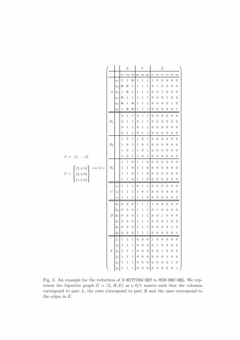
Proof. We prove the hardness with a reduction from the following APX-hardproblem, called 3-HITTING-SET [12]: Given a family F of subsets of size 3 ofa finite set S such that each element of S is covered by at most 3 sets, find aset S ′ ⊆ S of minimum cardinality that intersects all members of F .

Let I = (F , S) be an instance of 3-HITTING-SET with S = {1, . . . , n}and F = {T1, . . . , Tm}. Moreover, we assume that m ≥ 3. We construct anidentifiable bipartite graph G = (L, R; E) of size |L| = 2m + n and |R| =2m2 −m + 3n; an example for the construction is illustrated in Fig. 2. Thevertex set L consists of three parts: X = {x1, . . . , xm}, Y = {y1, . . . , ym} andZ = {z1, . . . , zn}. The vertex set R consists of m + 4 parts: A = {a1, . . . , an},

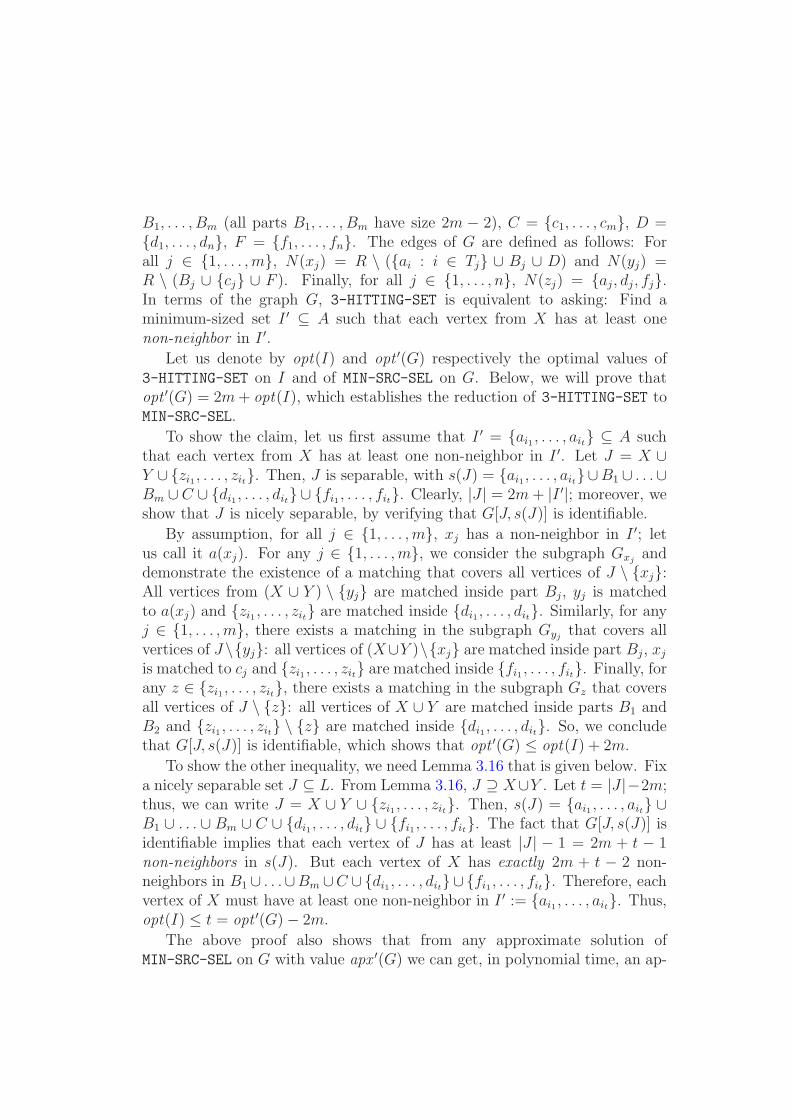
B1, . . . , Bm (all parts B1, . . . , Bm have size 2m − 2), C = {c1, . . . , cm}, D ={d1, . . . , dn}, F = {f1, . . . , fn}. The edges of G are defined as follows: Forall j ∈ {1, . . . , m}, N(xj) = R \ ({ai : i ∈ Tj} ∪ Bj ∪ D) and N(yj) =R \ (Bj ∪ {cj} ∪ F ). Finally, for all j ∈ {1, . . . , n}, N(zj) = {aj, dj, fj}.In terms of the graph G, 3-HITTING-SET is equivalent to asking: Find aminimum-sized set I ′ ⊆ A such that each vertex from X has at least onenon-neighbor in I ′.

Let us denote by opt(I) and opt ′(G) respectively the optimal values of3-HITTING-SET on I and of MIN-SRC-SEL on G. Below, we will prove thatopt ′(G) = 2m + opt(I), which establishes the reduction of 3-HITTING-SET toMIN-SRC-SEL.

To show the claim, let us first assume that I ′ = {ai1 , . . . , ait} ⊆ A suchthat each vertex from X has at least one non-neighbor in I ′. Let J = X ∪Y ∪ {zi1 , . . . , zit}. Then, J is separable, with s(J) = {ai1, . . . , ait}∪B1 ∪ . . .∪Bm ∪C ∪ {di1, . . . , dit} ∪ {fi1 , . . . , fit}. Clearly, |J | = 2m + |I ′|; moreover, weshow that J is nicely separable, by verifying that G[J, s(J)] is identifiable.

By assumption, for all j ∈ {1, . . . , m}, xj has a non-neighbor in I ′; letus call it a(xj). For any j ∈ {1, . . . , m}, we consider the subgraph Gxj

anddemonstrate the existence of a matching that covers all vertices of J \ {xj}:All vertices from (X ∪ Y ) \ {yj} are matched inside part Bj, yj is matchedto a(xj) and {zi1 , . . . , zit} are matched inside {di1, . . . , dit}. Similarly, for anyj ∈ {1, . . . , m}, there exists a matching in the subgraph Gyj

that covers allvertices of J \{yj}: all vertices of (X∪Y )\{xj} are matched inside part Bj, xj

is matched to cj and {zi1 , . . . , zit} are matched inside {fi1 , . . . , fit}. Finally, forany z ∈ {zi1 , . . . , zit}, there exists a matching in the subgraph Gz that coversall vertices of J \ {z}: all vertices of X ∪ Y are matched inside parts B1 andB2 and {zi1 , . . . , zit} \ {z} are matched inside {di1 , . . . , dit}. So, we concludethat G[J, s(J)] is identifiable, which shows that opt ′(G) ≤ opt(I) + 2m.

To show the other inequality, we need Lemma 3.16 that is given below. Fixa nicely separable set J ⊆ L. From Lemma 3.16, J ⊇ X∪Y . Let t = |J |−2m;thus, we can write J = X ∪ Y ∪ {zi1 , . . . , zit}. Then, s(J) = {ai1 , . . . , ait} ∪B1 ∪ . . . ∪ Bm ∪ C ∪ {di1, . . . , dit} ∪ {fi1 , . . . , fit}. The fact that G[J, s(J)] isidentifiable implies that each vertex of J has at least |J | − 1 = 2m + t − 1non-neighbors in s(J). But each vertex of X has exactly 2m + t − 2 non-neighbors in B1 ∪ . . .∪Bm ∪C ∪{di1, . . . , dit}∪ {fi1 , . . . , fit}. Therefore, eachvertex of X must have at least one non-neighbor in I ′ := {ai1 , . . . , ait}. Thus,opt(I) ≤ t = opt ′(G)− 2m.

The above proof also shows that from any approximate solution ofMIN-SRC-SEL on G with value apx ′(G) we can get, in polynomial time, an ap-

proximate hitting set on I with value apx (I) such that apx(I) = apx ′(G)−2m.So, we get apx (I)−opt(I) = apx ′(G)−opt ′(G) and opt ′(G) = 2m+ opt(I) ≤7opt(I) (since each element x ∈ S is covered by at most 3 sets in I, we getopt(I) ≥ m/3). Thus, the reduction is an L-reduction and the result follows.

2

Lemma 3.16 If J ⊆ L is a nicely separable set in G, then J ⊇ X ∪ Y .

Proof. First we show the following statements:

∀j ∈ {1, . . . , m} : yj ∈ J ⇒ J ⊇ X \ {xj} (1)

∀j ∈ {1, . . . , m} : xj ∈ J ⇒ J ⊇ Y \ {yj} (2)

Because J is nicely separable, there exists a set s(J) ⊆ R such thatN(s(J)) = J and G[J, s(J)] is identifiable. Let us assume that yj ∈ J ; thenthe identifiability of G[J, s(J)] implies that s(J) contains at least one non-neighbor of yj. But every non-neighbor of yj is connected to all vertices ofX \ {xj}. Therefore, N(s(J)) ⊇ X \ {xj} and (1) follows. Similarly, we canshow (2).

Now, we show that if J contains any vertex from X ∪ Y , then it containsthem all. Thereby, we make use of the assumption that m ≥ 3. Without lossof generality we assume that x1 ∈ J and from (1) and (2) we get the followingsequence of implications:

x1 ∈ J ⇒ J ⊇ Y \ {y1} ⇒ y2 ∈ J

y2 ∈ J ⇒ J ⊇ X \ {x2} ⇒ x3 ∈ J

x3 ∈ J ⇒ J ⊇ Y \ {y3} ⇒ y1 ∈ J

y1 ∈ J ⇒ J ⊇ X \ {x1} ⇒ x2 ∈ J

So, it follows that J ⊇ X ∪ Y .

To complete the proof, it remains to show that J contains at least onevertex from X ∪ Y . For the sake of contradiction, suppose that there is anicely separable set J ⊆ Z. The identifiability of G[J, s(J)] implies that foreach x ∈ J , s(J) contains at least one vertex that is connected to x. Butfor every y ∈ Z, every vertex that is connected to y is also connected to avertex from X ∪ Y . Therefore, N(s(J)) ∩ (X ∪ Y ) 6= ∅ and this implies thatJ ∩ (X ∪ Y ) 6= ∅, which is a contradiction. 2

References

[1] Berge, C., Two theorems in graph theory, Proc. Natl. Acad. Sci. USA 43 (1957),pp. 842–844.

[2] Bondy, J. A. and U. S. R. Murty, “Graph Theory.” Graduate Texts inMathematics 244, Springer, New York, 2008.

[3] Boscolo, R., C. Sabatti, J. Liao and V. Roychowdhury, A generalized framework

for network component analysis., IEEE Trans. Comp. Biol. Bioinf. 2 (2005),pp. 289–301.

[4] Diestel, R., “Graph Theory, Third Edition,” Springer, 2005.

[5] Fritzilas, E., Y. Rios-Solis and S. Rahmann, Structural identifiability in low-

rank matrix factorization, in: Proceedings of COCOON’08, LNCS 5092, 2008,pp. 140–148, Extended version:http://www.cebitec.uni-bielefeld.de/∼efritzil/papers/IdentifiableGraphs.pdf.

[6] Hall, P., On representatives of subsets, J. London Math. Society 10 (1935),pp. 26–30.

[7] Hopcroft, J. and R. Karp, An n5/2 algorithm for maximum matchings in

bipartite graphs, SIAM J. Comput. 2 (1973), pp. 225–231.

[8] Iwata, S., A faster scaling algorithm for minimizing submodular functions,SIAM J. Comput. 32 (2003), pp. 833–840.

[9] Liao, J., R. Boscolo, Y.-L. Yang, L. Tran, C. Sabatti and V. Roychowdhury,Network component analysis: reconstruction of regulatory signals in biological

systems., Proc. Natl. Acad. Sci. USA 100 (2003), pp. 15522–15527.

[10] Lovasz, L. and M. Plummer, “Matching Theory,” North-Holland, 1986.

[11] Orlin, J. B., A faster strongly polynomial time algorithm for submodular

function minimization, in: Proceedings of IPCO’07, LNCS 4513, 2007, pp. 240–251.

[12] Papadimitriou, C. and M. Yannakakis, Optimization, approximation, and

complexity classes, J. Comput. Syst. Sci. 43 (1991), pp. 425–440.

[13] Robertson, N. and P. Seymour, Graph minors. XIII. the disjoint paths problem,J. Comb. Theory, Ser. B 63 (1995), pp. 65–110.

[14] Wang, H., E. Hubbell, J. Hu, G. Mei, M. Cline, G. Lu, T. Clark, M. Siani-Rose, M. Ares, D. Kulp and D. Haussler, Gene structure-based splice variant

deconvolution using a microarray platform, Bioinformatics 19 (2003), pp. i315–i322.

S = {1, . . . , 6}

F =

8

>

>

>

<

>

>

>

:

{2, 4, 5}

{2, 3, 6}

{1, 5, 6}

9

>

>

>

=

>

>

>

;

=⇒ G =

0

B

B

B

B

B

B

B

B

B

B

B

B

B

B

B

B

B

B

B

B

B

B

B

B

B

B

B

B

B

B

B

B

B

B

B

B

B

B

B

B

B

B

B

B

B

B

B

B

B

B

B

B

B

B

B

B

B

B

B

B

B

B

B

B

B

B

B

B

B

B

B

B

B

B

B

B

B

B

B

B

B

B

B

B

B

B

B

B

B

B

B

B

B

B

B

B

B

B

B

B

@

X Y Z

x1 x2 x3 y1 y2 y3 z1 z2 z3 z4 z5 z6

a1 1 1 0 1 1 1 1 0 0 0 0 0

a2 0 0 1 1 1 1 0 1 0 0 0 0

A a3 1 0 1 1 1 1 0 0 1 0 0 0

a4 0 1 1 1 1 1 0 0 0 1 0 0

a5 0 1 0 1 1 1 0 0 0 0 1 0

a6 1 0 0 1 1 1 0 0 0 0 0 1

0 1 1 0 1 1 0 0 0 0 0 0

B1 0 1 1 0 1 1 0 0 0 0 0 0

0 1 1 0 1 1 0 0 0 0 0 0

0 1 1 0 1 1 0 0 0 0 0 0

1 0 1 1 0 1 0 0 0 0 0 0

B2 1 0 1 1 0 1 0 0 0 0 0 0

1 0 1 1 0 1 0 0 0 0 0 0

1 0 1 1 0 1 0 0 0 0 0 0

1 1 0 1 1 0 0 0 0 0 0 0

B3 1 1 0 1 1 0 0 0 0 0 0 0

1 1 0 1 1 0 0 0 0 0 0 0

1 1 0 1 1 0 0 0 0 0 0 0

c1 1 1 1 0 1 1 0 0 0 0 0 0

C c2 1 1 1 1 0 1 0 0 0 0 0 0

c3 1 1 1 1 1 0 0 0 0 0 0 0

d1 0 0 0 1 1 1 1 0 0 0 0 0

d2 0 0 0 1 1 1 0 1 0 0 0 0

D d3 0 0 0 1 1 1 0 0 1 0 0 0

d4 0 0 0 1 1 1 0 0 0 1 0 0

d5 0 0 0 1 1 1 0 0 0 0 1 0

d6 0 0 0 1 1 1 0 0 0 0 0 1

f1 1 1 1 0 0 0 1 0 0 0 0 0

f2 1 1 1 0 0 0 0 1 0 0 0 0

F f3 1 1 1 0 0 0 0 0 1 0 0 0

f4 1 1 1 0 0 0 0 0 0 1 0 0

f5 1 1 1 0 0 0 0 0 0 0 1 0

f6 1 1 1 0 0 0 0 0 0 0 0 1

1

C

C

C

C

C

C

C

C

C

C

C

C

C

C

C

C

C

C

C

C

C

C

C

C

C

C

C

C

C

C

C

C

C

C

C

C

C

C

C

C

C

C

C

C

C

C

C

C

C

C

C

C

C

C

C

C

C

C

C

C

C

C

C

C

C

C

C

C

C

C

C

C

C

C

C

C

C

C

C

C

C

C

C

C

C

C

C

C

C

C

C

C

C

C

C

C

C

C

C

C

A

Fig. 2. An example for the reduction of 3-HITTING-SET to MIN-SRC-SEL. We rep-resent the bipartite graph G = (L,R;E) as a 0/1 matrix such that the columnscorrespond to part L, the rows correspond to part R and the ones correspond tothe edges in E.