Matching oversegmented 3D images to models using association graphs

Matching oversegmented 3D images to models using

association graphs

B Yang, W E Snyder and G L Bilbro

A new enhun~ement to the use of ussuciut~on graphs ,for model matching is introduced. The specific problem uddressed is matching when, due to noise, errors occur in the segmentation process, and these errors result in oversegmentation: that is, a single surface in the model is reported as two surfaces by the segmenter. The ussocia- tion graph is augmented by ‘merge nodes’ which possess the appropriate properties. The ff~gorithrn is des&r~bed and examples are presented.

Keywords: association graphs, oversegmentation, matching, segmentation errors

Since 1983 researchers at North Carolina State Univer- sity, USA have been developing computer algorithms for the analysis of three-dimensional images. By the authors’ definition, a three-dimensional image is a two- dimensional array of numbers in which each number represents a distance to a point on a surface. In the special case of a depth image, the distance referred to in the definition is the perpendicular distance from a point on the surface to an arbitrary reference plane. That plane is generally chosen to be coincident with the focal plane of the camera, allowing a depth image to be defined in the form of z(x,~).

As in traditional luminance imagery, the first step in analysis of depth images is to segment the image into homogeneous regions. In this case ‘similar surface curvature’ is used as the operational definition of homogeneous. The authors have spent considerable effort in the past developing strategies for good segmentation’. Once a segmentation of a depth image has been produced, that se~entation is immediately abstracted and an augmented region adjacency graph2 is produced which is referred to as a ‘scene graph’.

In order to recognize the object, the observed model graph is then matched to the scene graph. It is that model matching process which is the topic of this paper.

Center for Communications and Signal Processing, North Carolina State University, PO Box 7914, Raleigh, NC 27695-7914, USA

In the absence of noise or other segmentation defects, the scene graph will be a proper subgraph of the model graph and subgraph isomorphism will, at least in theory, be sufficient to match the graphs. Although some excel- lent speed-up heuristics 3,4 have been developed, the solution to a subgraph isomorphism problem requires computation time which is exponential in the number of nodes. However, such complexity is not the major objection to formal subgraph isomo~hism as a matching technique but rather the fact that subgraph isomorphism is totally intolerant to any errors which might occur in the segmentation.

It is useful to refer to nodes in the model graph as “regions’ and to nodes in the scene graph as ‘patches’. If a segmenter performs optimally, the scene graph is isomorphic to a subgraph of the model graph. How- ever,the segmenter may fail. Segmentation errors may be of two types. The first, ‘undersegmentation’ or ‘region blending’, produces a scene graph in which two or more regions are combined into the same patch. Region blending generally occurs when noise or artifacts blur an edge such that a gap occurs in the edge and connected compo- nent labelling combines the two. The second type of failure, ‘oversegmentation’ occurs when noise induced spurious edges fragment a single region into more than one patch.

One may ‘tune’ a segmenter to favour one type of error over another. For example, by lowering the thres- hold of an edge detector, one may encourage fragmentation and produce few, if any, blends. In this paper, it is assumed that this has been done and this segmenter fails only by oversegmentation.

To alleviate some of the sensitivity problems with subgraph isomorphism, the theory of association graphs was developed. The idea of matching models to images by matching the corresponding graph-theoretic descriptions was first developed by Ambler5 and used by several other researchers6,‘. The ideas are well formulated and the literature surveyed in Radig’sa work.

One early paperg which utilized association graphs for feature matching was presented in 1979. In that paper, the author used the following strategy: first, res-

0262-8856/89/020135-09 $03.00 @ 1989 Butterworth &Co. (Publishers) Ltd

~017 no 2 Ma?, 1989 135

trict the model to key features; second, use geometric limits with respect to some feature to exclude features; and third, iteratively apply the maximal clique method to refine an assignment. The geometric limit used was Euclidian distance between features.

Radig7 establishes a formal framework for describing relational structures such as association graphs. In his formalism, Radig allows the use of more than one relation whereas in this work only one binary relation (adjacency of the patches) is presented.

cl 0 a

Jacobus, Chien and Selander’O use a different approach to graph matching. A ‘half-chunk’ (H-C) graph is generated by using a set of unary relations which comes from geometrical types and characteristics. A cost function determines the most compatible matching between two H-C graphs.

2 b

The fact that matching of graphs is really a problem in consistent labelling has been obseved by several researchers’ 1-l 2,1 3.

In Davis’ paper14 a spring function is defined to be the mapping 0 x T - G. The concept of augmented association graph (they call it augmented network) is introduced in order to apply relaxation techniques. The augmented association graph is used here to find the best match between the model and segmented image scene graphs by creating new nodes in the original association graph to increase consistency. Mapping is defined by consistency based on the adjacency of the patches.

77 3

Model

u C

image

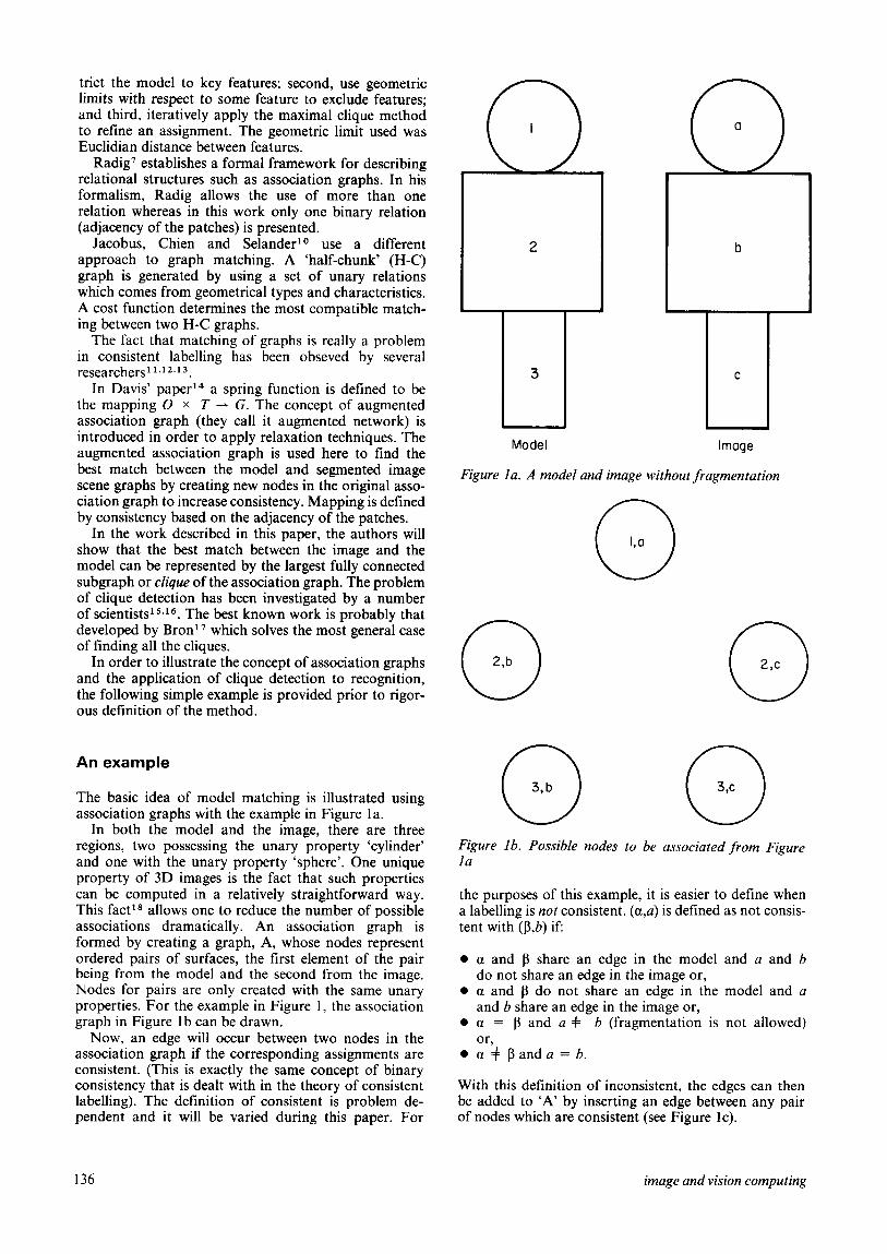
Figure la. A model and image without fragmentation

In the work described in this paper, the authors will show that the best match between the image and the model can be represented by the largest fully connected subgraph or clique of the association graph. The problem of clique detection has been investigated by a number of scientists15,16. The best known work is probably that developed by Broni7 which solves the most general case of finding all the cliques.

0 Ita

In order to illustrate the concept of association graphs and the application of clique detection to recognition, the following simple example is provided prior to rigor- ous definition of the method.

An example

The basic idea of model matching is illustrated using association graphs with the example in Figure la.

In both the model and the image, there are three regions, two possessing the unary property ‘cylinder’ and one with the unary property ‘sphere’. One unique property of 3D images is the fact that such properties can be computed in a relatively straightforward way. This fact’* allows one to reduce the number of possible associations dramatically. An association graph is formed by creating a graph, A, whose nodes represent ordered pairs of surfaces, the first element of the pair being from the model and the second from the image. Nodes for pairs are only created with the same unary properties. For the example in Figure 1, the association graph in Figure lb can be drawn.

Figure lb. Possible nodes to be associated from Figure la

the purposes of this example, it is easier to define when a labelling is not consistent. (a,a) is defined as not consistent with (P,b) if:

Now, an edge will occur between two nodes in the association graph if the corresponding assignments are consistent. (This is exactly the same concept of binary consistency that is dealt with in the theory of consistent labelling). The definition of consistent is problem de- pendent and it will be varied during this paper. For

l a and p share an edge in the model and a and b do not share an edge in the image or,

l a and l3 do not share an edge in the model and a and b share an edge in the image or,

l a = p and a + b (fragmentation is not allowed)

l z”$ l3 and a = 6.

With this definition of inconsistent, the edges can then be added to ‘A’ by inserting an edge between any pair of nodes which are consistent (see Figure lc).

136 image and vision computing

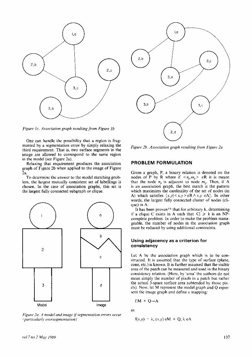
Figure lc. Association graph resulting from Figure lb

One can handle the possibility that a region is frag- mented by a segmentation error by simply relaxing the third requirement. That is, two surface segments in the image are allowed to correspond to the same region in the model (see Figure 2a).

Relaxing that requirement produces the association graph of Figure 2b when applied to the image of Figure 2a.

To determine the answer to the model matching problem, the largest mutually consistent set of labellings is chosen. In the case of association graphs, this set is the largest fully connected subgraph or clique.

(7 2,d

Figure 2b. Association graph resulting.from Figure 2a

PROBLEM FORMULATION

Given a graph, P, a binary relation is denoted on the nodes of P by R where if <n,,m,> ER it is meant that the node nP is adjacent to node m,. Then, if A is an association graph, the best match is the pattern which maximizes the cardinality of the set of nodes (in A) which satisfies {x,yl < x,y > ER A x,y EA}. In other words, the largest fully connected cluster of nodes (clique) in A.

It has been proven lg that for arbitrary k, determining if a clique C exists in A such that ICI 3 k is an NP- complete problem. In order to make the problem mana- geable, the number of nodes in the association graph must be reduced by using additional constraints.

Model Image as

Using adjacency as a criterion for consistency

Let A be the association graph which is to be constructed. It is assumed that the type of surface (plane, cone, etc.) is known. It is further assumed that the visible area of the patch can be measured and used in the binary consistency relation. (Here, by ‘area’ the authors do not mean simply the number of pixels in a patch but rather the actual 3-space surface area subtended by those pixels). Now, let M represent the model graph and Q represent the image graph and define a mapping:

Figure 2~. A model and image if segmentation errors occur (particularly over-segmentation) f(x,y) = h, (XJ) EM x Q, h EA

vol7 no 2 May 1989 137

and for

CGY) + (48 -f Cw) + f (id

Here, A denotes the association graph being constructed. Here, the domain of

M x Q = {(X&X EM, JKZQ A TYPE(x) = TYPE@) A AREA(x) > AREA(

The function f, therefore, is used to build the association graph.

The relation R has been defined as representing the fact that two nodes in a graph are adjacent. That definition can easily be extended to allow a binary relation by the same name, defined on A, and interpreted as meaning that two nodes in the association graph share an edge. Thus, a mapping is defined R, x R,+R,, by defining the concept of consistency. Two nodes in the association graph ij E A are said to be consistent if < ij > ERR and inconsistent if < ij > $RA, where

R, = { < ij > l(ij EA) and i is adjacent to j}

Similarly, R, and R, can be defined as adjacency relations.

Later in this section, the association graph will be augmented by adding a node which represents the merge of two previous nodes. To facilitate discussion of this topic, the concept of an indirect node is introduced. If r is an indirect node created by merging, for example, nodes p and q, one says p cr and q cr. Then, the mapping R, x R, --) R, is defined as:

Let i = f (p, m), j = f(q,n)

where p, q E M, m,nEQ, and i,jEA. Further, let R,, R,, and R, represent adjacency relations. The following are defined: first, nodes i and j are ‘consistent, type 1’ iff

m$nAn&mA <p,q>ERMA < m,n > ERR+ < ij > ER*.

Second, nodes i and j are ‘consistent, type 2’ iff

< p,q > $R, A < m,n > $R,+ < ij > ERR.

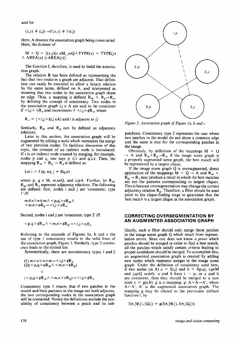
Referring to the example of Figures la, b and c the use of type 1 consistency results in the solid lines of the association graph, Figure 3. Similarly, type 2 consistency leads to the dotted line.

Symmetrically, there are inconsistency types 1 and 2:

(1) mcnVncm+<i,j>$R, (2)( < p,q > eRM A < m,n > We)

V

(< p,q > $RM A < m,n > ERJ+ < ij > #RA.

Consistency type 1 means that if two patches in the model and their partners in the image are both adjacent, the two corresponding nodes in the association graph will be connected. Notice the definitions exclude the possibility of consistency between a patch and its sub-

Figure 3. Association graph of Figure la, b and c

patch(es). Consistency type 2 represents the case where two patches in the model do not share a common edge and the same is true for the corresponding patches in the image.

Obviously, by definition of the mappings M x Q + A and R,x R,+R,, if the image scene graph is a properly segmented scene graph, the best match will be represented by a largest clique.

If the image scene graph Q is oversegmented, direct application of the mappings M x Q + A and R, x R, + R, may produce a result in which the best matches are not the patterns corresponding to largest cliques. This is because oversegmentation may change the correct adjacency relation R,. Therefore, a filter should be used prior to the clique-finding stage to guarantee that the best match is a largest clique in the association graph.

CORRECTING OVERSEGMENTATION BY AN AUGMENTED ASSOCIATION GRAPH

Ideally, such a filter should only merge those patches in the image scene graph Q which result from segmentation errors. Since one does not know a priori which patches should be merged in order to find a best match, all the patches which satisfy certain criteria leading to proper candidates should be merged. To accomplish this, an augmented association graph is created by adding new nodes which represent merges in the image scene graph. Under the definition of consistency used here, if two nodes (in A) a = f(ij) and b = f(p,q), i,peM and j,qEQ satisfy: a and b have i = p; or a and b are consistent, then they should be merged to a new node c = g(a,b). g is a mapping: g: A x A+A’, where A c A’, A’ is the augmented association graph. The mapping g may be related to the previously defined function f, by


The mapping g may be applied recursively so that a merge node potentially represents a set of patches rather than simply a pair. Hence, set notation is used to denote merge nodes.

From the definition above, the mapping g has the following properties (formal proofs may be found in a working paper by Ben Yang20).

Theorem 1: The cardinality of the largest cliques in A’ will not be increased by improperly merging two nodes in A. This is simply because improper merging cannot improve consistency based on adjacency.

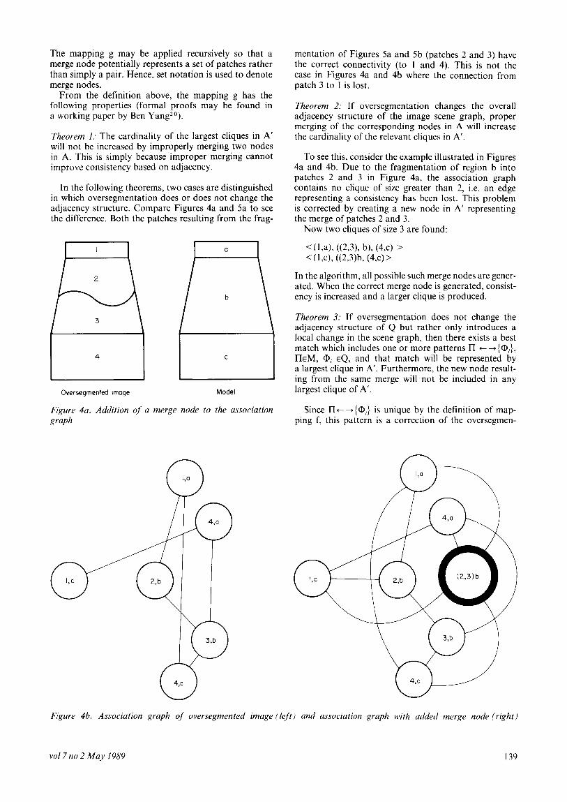
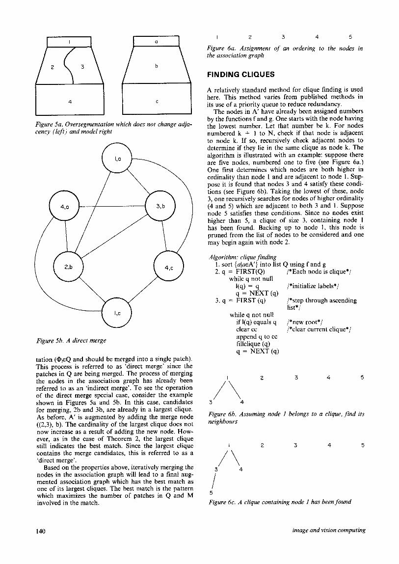
In the following theorems, two cases are distinguished in which oversegmentation does or does not change the adjacency structure. Compare Figures 4a and 5a to see the difference. Both the patches resulting from the frag-

C

Oversegmented fmoge Model

Figure 4a. Addition Qf a merge node to the association graph

Figure 4h. Association graph of oversegmented image (left) and association graph with added merge node (right)

~017 no 2 May 1989 139

mentation of Figures 5a and 5b (patches 2 and 3) have the correct connectivity (to 1 and 4). This is not the case in Figures 4a and 4b where the connection from patch 3 to 1 is lost.

Theorem 2: If oversegmentation changes the overall adjacency structure of the image scene graph, proper merging of the corresponding nodes in A will increase the cardinality of the relevant cliques in A’.

To see this, consider the example illustrated in Figures 4a and 4b. Due to the fragmentation of region b into patches 2 and 3 in Figure 4a, the association graph contains no clique of size greater than 2, i.e. an edge representing a consistency has been lost. This problem is corrected by creating a new node in A’ representing the merge of patches 2 and 3.

Now two cliques of size 3 are found:

< (1 ,a), ((2,3), b), (4,~) > < ( 1~1, ((23x (4,~) >

In the algorithm, all possible such merge nodes are generated. When the correct merge node is generated, consistency is increased and a larger clique is produced.

Theorem 3: If oversegmentation does not change the adjacency structure of Q but rather only introduces a local change in the scene graph, then there exists a best match which includes one or more patterns l7 c -+ ((D;), HEM, @, EQ, and that match will be represented by a largest clique in A’. Furthermore, the new node resulting from the same merge will not be included in any largest clique of A’.

Since Ht -{(I),} is unique by the definition of mapping f, this pattern is a correction of the oversegmen-

I 2 3 4 5

Figure 6a. Assignment C$ an ordering to the nodes in the association graph

FINDING CLIQUES

4 C

A relatively standard method for clique finding is used here. This method varies from published methods in its use of a priority queue to reduce redundancy.

The nodes in A’ have already been assigned numbers

Figure 5a. ~ver~egmentat~on which dues not change adjacency (left) and model right

by the functions f and g. One starts with the node having the lowest number. Let that number be k. For nodes numbered k + 1 to N, check if that node is adjacent to node k. If so, recursively check adjacent nodes to determine if they lie in the same clique as node k. The algorithm is illustrated with an example: suppose there are live nodes, numbered one to five (see Figure 6a.) One first determines which nodes are both higher in ordinality than node 1 and are adjacent to node 1. Sup- pose it is found that nodes 3 and 4 satisfy these conditions (see Figure 6b), Taking the lowest of these, node 3, one recursively searches for nodes of higher ordinality (4 and 5) which are adjacent to both 3 and 1. Suppose node 5 satisfies these conditions. Since no nodes exist higher than 5, a clique of size 3, containing node 1 has been found. Backing up to node 1, this node is pruned from the list of nodes to be considered and one may begin again with node 2.

Algorithm: clique finding 1. sort (alaeA’) into list Q using f and g 2. q = FIRST(Q) /*Each node is clique*/

while q not null l(q) = q /*initialize labels*/ q = NEXT (q)

3. q = FIRST (q) /*step through ascending list*/

while q not null if l(q) equals q /*new root*/ clear cc /*clear current clique*/

Figure 5b. A direct merge

tation (@,EQ and should be merged into a single patch). This process is referred to as ‘direct merge’ since the patches in Q are being merged. The process of merging the nodes in the association graph has already been referred to as an ‘indirect merge’. To see the operation of the direct merge special case, consider the example shown in Figures 5a and 5b. In this case, candidates for merging, 2b and 3b, are already in a largest clique. As before, A’ is augmented by adding the merge node ((2,3), b). The cardinality of the largest clique does not now increase as a result of adding the new node. How- ever, as in the case of Theorem 2, the largest clique still indicates the best match. Since the largest clique contains the merge candidates, this is referred to as a ‘direct merge’.

Based on the properties above, iteratively merging the nodes in the association graph will lead to a final augmented association graph which has the best match as one of its largest cliques. The best match is the pattern which maximizes the number of patches in Q and M involved in the match.

append q to cc fillclique (q) q = NEXT(q)

I 2 3

A 3 4

4 5

Figure 6b. Assuming node I belongs to a clique, find its neighbours

2 3 4

A 3 4

I i

Figure 6c. A clique containing node I has been found


0 fillclique (q)

r = NEXT(q) while r not null

if inclique (q,r) l(r) = l(q) append r to cc tillclique (r)

r = NEXT (q) l inclique (q,r)

p = FIRST(cc)

while p not null

/*label all member of q’s clique*/

/*assign r to q’s clique*/

/*is r adjacent to q’s clique*/ /*will test against every node in q’s clique*/

if not adjcaent (r,p) RETURN FALSE

p = NEXT (p) RETURN TRUE /*r is adjacent to every

node*/ /*known to be in q’s clique*/

This algorithm is standard depth-first-search with NP- complete performance. Checking the ancestor of a node is accelerated by keeping the current clique on list cc.

EXAMPLES

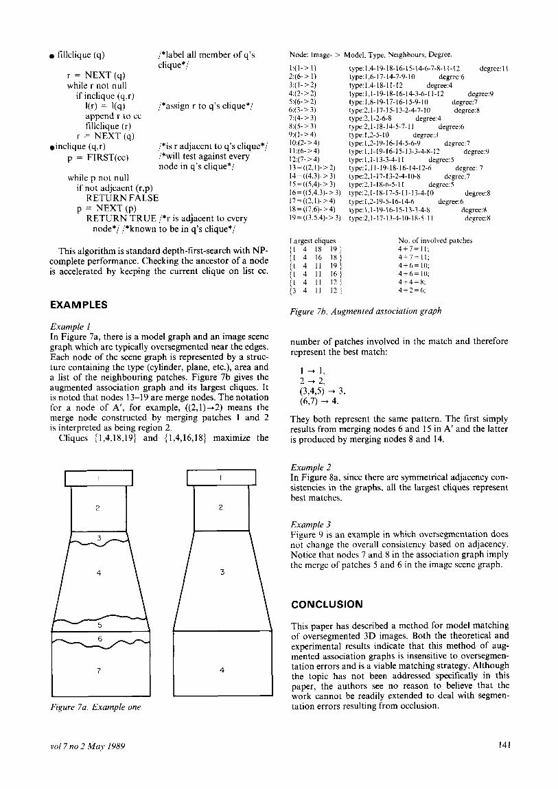
Example 1 In Figure 7a, there is a model graph and an image scene graph which are typically oversegmented near the edges. Each node of the scene graph is represented by a structure containing the type (cylinder, plane, etc.), area and a list of the neighbouring patches. Figure 7b gives the augmented association graph and its largest cliques. It is noted that nodes 13-19 are merge nodes. The notation for a node of A’, for example, ((2,1)+2) means the merge node constructed by merging patches 1 and 2 is interpreted as being region 2.

Cliques { 1,4,18,19} and (1,4,16,18) maximize the

1 I 1 2

Figure 7a. Example one

~017 no 2 May I989

Node: Image- > Model, Type, Neighbours, Degree.

l:(I-> 1) type: 1.4-19-18-16-15-14-6-7-8-1 I- 12 degree: 11 2:(6- > 1) type: 1,6-17-14-7-9-10 degree:6 3:(1->2) type:1,4-18-1 l-12 degree:4 4:(2- > 2) type:l,l-19-18-16-14-3-6-l l-12 degree:9 5:(6- > 2) type:l,8-19-17-16-15-9-10 degree:7 6:(3- > 3) type:2,1-17-15-13-2-4-7-10 degree:8 7:(4- > 3) type:,, 1-2-6-8 degree:4 8:(5- > 3) type:2,1-18-14-5-7-11 degree:6 9:(1->4) type:1,2-5-10 degree:3 10:(2- > 4) type: 1,2-19-16-14-5-6-9 degree:7 11:(6-~4) type:l.l-19-16-15-13-3-4-8-12 degree:9 12:(7-14) type:l,l-13-3-4-11 degree:5 13=((2,1)->2) type:l,ll-19-18-16-14-12-6 degree: 7 14= ((4,3)- > 3) type:2,1-17-13-2-4-10-8 degree:7 15 = ((5,4)- > 3) type:2,1-18-6-5-11 degree:5 16=((5,4,3)->3) type:2,1-18-17-5-II-13-4-10 degree:8 17=((2,1)->4) type:1.2-19-5-16-14-6 degree:6 18=((7,6)->4) type:l,l-19-16-15-13-3-4-8 degree:8 19=((3,5,4)->3) type:2,1-17-13-4-10-18-5-l I degree:8

Largest cliques No. of involved patches {I 4 18 19) 4+7=11; iI 4 16 18 ) 4+7=11; {I 4 11 19) 4+6= 10; {l 4 11 16) 4+6= 10; {1 4 II 12) 4+4=8; {3 4 11 12 ) 4+2=6:

Figure 7b. Augmented association graph

number of patches involved in the match and therefore represent the best match:

1 -+ 1, 2 + 2, (3,455) -+ 3, (6,7) + 4.

They both represent the same pattern. The first simply results from merging nodes 6 and 15 in A’ and the latter is produced by merging nodes 8 and 14.

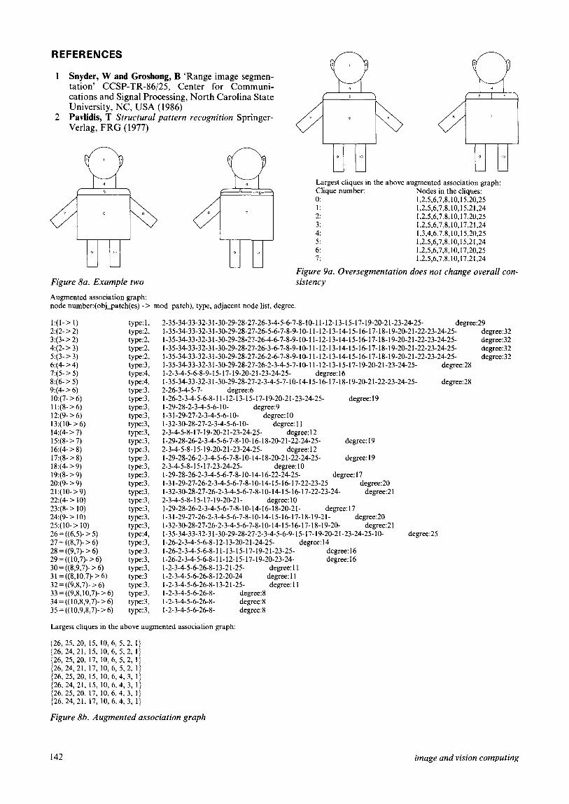
Example 2 In Figure 8a, since there are symmetrical adjacency con- sistencies in the graphs, all the largest cliques represent best matches.

Example 3 Figure 9 is an example in which oversegmentation does not change the overall consistency based on adjacency. Notice that nodes 7 and 8 in the association graph imply the merge of patches 5 and 6 in the image scene graph.

CONCLUSION

This paper has described a method for model matching of oversegmented 3D images. Both the theoretical and experimental results indicate that this method of augmented association graphs is insensitive to oversegmentation errors and is a viable matching strategy. Although the topic has not been addressed specifically in this paper, the authors see no reason to believe that the work cannot be readily extended to deal with segmentation errors resulting from occlusion.

141

1 Snyder, W and Groshong, B ‘Range image segmentation’ CCSP-TR-86/25, Center for Communi- cations and Signal Processing, North Carolina State University, NC, USA (1986)

2 Pavlidis, T Structural pattern recognition Springer- Verlag, FRG (1977)

Figure 8a. Example two

Augmented association graph: node number:(obj_patch(es) - > mod-patch), type, adjacent node list, degree.

l:(l-> I) 2:(2- > 2) 3:(3- > 2) 4:(2- > 3) 5:(3- > 3) 6:(4- > 4) 7:(5- > 5) 8:(6- > 5) 9:(4- > 6) l&(7->b) 11:(8- > 6) 12:(9- > 6) 13:(10->6) 14:(4->7)’ 15:(8- > 7) 16:(4- r 8) 17:(8- > 8) 18:(4- > 9j 19:(8-z 9) 20:(9- > 9) 21:(10->9) 22:(4- > 10) 23:(8- > IO) 24:(9- 110) 25:(10-> 10) 26 = ((6,5)- > 5) 27 = ((8,7)- > 6) 28 = ((9,7)- > 6) 29 = (( 10,7)- > 6) 30 = ((8,9,7)- > 6) 31=((8,10,7)->6) 32 = ((9,8,7)- > 6) 33 = ((9,8,10,7)- > 6) 34=((10,8,9,7)->6) 35 = ((10,9,8,7)- > 6)

type: 1, type:2, type:2, type:2, type:2,

type:3, type:4, type:4, type:3, type:3, type:3, type:3,

type:3, type:3, type:3, type:3, type:3, type:3, type:3, type:3, type:3, type:3, type:3, type:3,

type:3, type:4, type:3, type:3, type:3,

type:5 type: 3 type:3, type:3, type:3, type:3,

Largest cliques in the above augmented association graph: Clique number: Nodes in the cliques: 0: 1 2 5 6 7 8 10,15,20,25 >?>1)1 1: 1 2 5 6 7 8 10,15,21,24 1 3 , , 3 9 2: 1 2 5 6 7 8 10,17,20,25 7 3 9 3 3 3 3: 1 2 5 6 7 8 10,17,21,24 T>,,,, 4: 1 3 4 6 7 8 10,15,20,25 ??,,,, 5: 12 5 6 7 8 10,15,21,24 1>1,1> 6: 1 2 5 6 7 8 10,17,20,25 ?>1,>, 7: 1,2,5,6,7,8,10,17,21,24

Figure 9a. Oversegmentation does not change overall consistency

2-35-34-33-32-31-30-29-28-27-26-3-4-5-6-7-8-10-l 1-12-13-15-17-19-20-21-23-24-25- degree:29 1-35-34-33-32-31-30-29-28-27-26-5-6-7-8-9-10-1~-12-13-14-15-16-17-18-19-20-21-22-23-24-25- degree:32 1-35-34-33-32-31-30-29-28-27-26-4-6-7-8-9-10-11-12-13-14-15-16-17-18-19-20-21-22-23-2425- degree:32 1-35-34-33-32-31-30-29-28-27-26-3-6-7-8-9-10-11-12-13-14-15-16-17-18-19-20-21-22-23-24-25- degree:32 1-35-34-33-32-31-30-29-28-27-26-2-6-7-8-9-10-l 1-12-13-14-15-16-17-18-19-20-21-22-23-24-25- degree:32 1-35-34-33-32-31-30-29-28-27-26-2-3-4-5-7-10-11-12-13-15-17-19-20-2~-23-24-25- degree:28 1-2-3-4-5-6-8-9-15-17-19-20-21-23-24-25- degree: 16 1-35-34-33-32-31-30-29-28-27-2-3-4-5-7-10-14-15-16-17-18-19-20-21-22-23-24-25- degree:28 2-26-3-4-5-7- degree:6 1-26-2-3-4-5-6-8-11-12-13-15-17-19-20-21-23-24-25- degree: 19 1-29-28-2-3-4-5-6-10- degree:9 l-3 l-29-27-2-3-4-5-6- lo- degree: 10 1-32-30-28-27-2-3-4-5-6-10- degree: 11 2-3-4-5-8-17-19-20-21-23-24-25- degree: 12 1-29-28-26-2-3-4-5-6-7-8-10-16-18-20-21-22-24-25- degree: 19 2-3-4-5-8-15-19-20-21-23-24-25- degree: 12 1-29-28-26-2-3-4-5-6-7-8-10-14-18-20-21-22-24-25- degree: 19 2-3-4-5-8-15-17-23-24-25- degree: 10 l-29-28-26-2-3-4-5-6-7-8-10-14-16-22-24-25- degree: 17 1-31-29-27-26-2-3-4-5-6-7-8-10-14-15-16-17-22-23-25 degree:20 1-32-30-28-27-26-2-3-4-5-6-7-8-10-14-15-16-17-22-23-24- degree:21 2-3-4-5-8-15-17-19-20-21- degree: 10 1-29-28-26-2-3-4-5-6-7-8-IO-14-16-l&20-21- degree: 17 1-31-29-27-26-2-3-4-5-6-7-8-10-14-15-16-17-18-19-21- degree:20 1-32-30-28-27-26-2-3-4-5-6-7-8-10-14-15-16-17-18-19-20- -degree:2 1 1-35-34-33-32-31-30-29-28-27-2-3-4-5-6-9-15-17-19-20-21-23-24-25-~0- 1-26-2-3-4-5-6-8-12-13-20-21-24-25- degree: 14 l-26-2-3-4-5-6-8-11-13-15-17-19-21-23-25- degree: 16

degree:25

1-26-2-3-4-5-6-8-11-12-15-17-19-20-23-24- 1-2-3-4-5-6-26-8-13-21-25- degree: 11 l-2-3-4-5-6-26-8-12-20-24 degree: 11 l-2-3-4-5-6-26-8-13-21-25- degree: I 1 1-2-3-4-5-6-26-8- degree:8 1-2-3-4-5-6-26-8- degree:8 1-2-3-4-5-6-26-8- degree:8

degree: 16

Largest cliques in the above augmented association graph:

(26, 25, 20, 15, 10, 6, 5, 2, 1 {26, 24, 21, 15, 10, 6, 5, 2, I {26, 25, 20, 17, 10, 6, 5, 2, I {26, 24, 21, 17, 10, 6, 5, 2, 1 (26, 25, 20, 15, 10, 6, 4, 3, 1 {26, 24, 21, 15, 10, 6, 4, 3, 1 126, 25, 20, 17, 10, 6,4, 3, 1 (26, 24, 21, 17, 10, 6, 4, 3, 1

Figure 8b. Augmented association graph


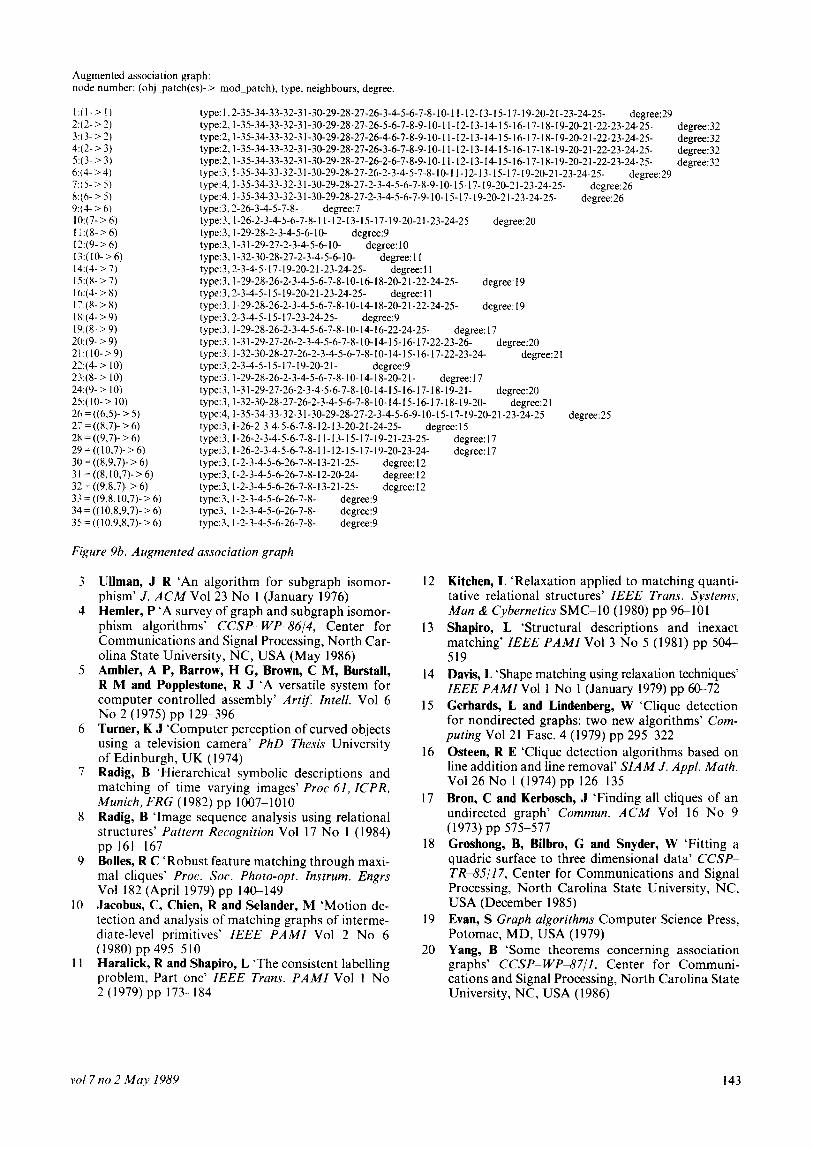
Augmented association graph: node number: (obj patch(es)- > mod-patch), type, neighbours, degree.

i:(i-2 1) 2:(2- > 2) 3:(3- > 2) 4:(2- > 3) 5:(3- > 3) 6:(3- > 4) 7:(5->5) 8:(6->5) 9:(3- > 6) 10:(7->6) 11:(8->6) 12:(9->6) 13:(10->6) 14:(4- > 7) IS:@->7) lh:(4->8) 17:(8->X) 1X:(4->9) 19:(8- > 9) 20:(9- > 9) 21:(10->9) 22:(4- > IO) 23:(8- > 10) 24:(9- > IO) 25:(10-> 10) 26 I ((6,5)-G 5) 2: = ((8,7)- > 6) 28 = ((9,7)- > 6) 29 =((10,7)->6) 30 = ((8,9,7)- > 6) 31 =((8,10,7)->6) 32 = ((9.8,7)- > 6) 37 = ((9,8,10,7)-> 6) 34=((10,8,9,7)->6) 35 = (( 10.9,8,7)- > 6)

type: 1,2-35-34-33-32-31-30-29-28-27-26-3-4-5-6-7-8-10-1 I-12-13-IS-17-l9-20-21-23-24-25- degree:29 type:2,1-35-34-33-32-31-30-29-28-27-26-5-6-7-8-9-lO-l l-l2-13-14-IS16-17-l8-l9-20-21-22-23-24-25- degree:32 type:2, 1-35-34-33-32-31-30-29-28-27-26-4-6-7-8-9-10-1l-12-l3-14-l5-16-l7-18-19-20-21-22-23-24-25- degree: 32 type:2,1-35-34-33-32-31-30-29-28-27-26-3-6-7-8-9-l0-~ l-12-l3-14-15-16-17-18-19-20-21-22-23-24-25- degree:32 type:2,1-35-34-33-32-31-30-29-28-27-26-2-6-7-8-9-10-1 I-12-13-14-15-16-17-18-19-20-21-22-23-24-25- degree:32 type:3,1-35-34-33-32-31-30-29-28-27-26-2-3-4-5-7-8-10-1 l-l2-13-15-17-19-20-21-23-24-25- degree:29 type:4, 1-35-34-33-32-31-30-29-28-27-2-3-4-5-6-7-8-9-10-15-l7-19-20-21-23-24-25- degree:26 type:4.1-35-34-33-32-31-30-29-28-27-2-3-4-5-6-7-9-lO-l5-17- 19-20-21-23-24-25- degree:26 type:3,2-26-3-4-5.7% degree:7 type:3,1-26-2-3-4-5-6-7-8-l l-12-13-15-17-19-20-21-23-24-25 degree:20 type:3,1-29-28-2-3-4-5-6-IO- degree:9 type:3, l-31-29-27-2-3-4-5-6-10- degree: 10 type:3.1-32-30-28-27-2-3-4-5-6-10- degree: 11 type:3.2-3-4-5-17-19-20-21-23-24-25- degree: 11 type:3,1-29-28-26-2-3-4-5-6-7-8-10-16-18-20-21-22-24-25- degree: 19 type:3,2-3-4-5-15-19-20-21-23-24-25- degree: 11 type:3,1-29-28-26-2-3-4-5-6-7-8-10-14-18-20-21-22-24-25- degree: 19 type:3,2-3-4-5-15-17-23-24-25- degree:9 type:3, l-29-28-26-2-3-4-5-6-7-8-10-14-16-22-24-25- degree: 17 type:3,1-31-29-27-26-2-3-4-5-6-7-8-10-14-15-16-17-22-23-26- degree:20 type:3,1-32-30-28-27-26-2-3-4-5-6-7-8-10-14-15-16-17-22-23-24- degree:21 type:3,2-3-4-5-15.17.19.20-21- degree:9 type:3. I-29-28-26-2-3-4-5-6-7-8-lo-l4-l8-20-21- degree: 17 type:3,1-31-29-27-26-2-3-4-5-6-7-8-10-14-15-16-l7-18-~9-21- degree:20 type:3,1-32-30-28-27-26-2-3-4-5-6-7-8-10-14-15-l6-l7-18-19-20- degree:2 1 type:4, 1-35-34-33-32-31-30-29-28-27-2-3-4-5-6-9-10-l5-l7-l9-20-21-23-24-25 degree:25 type:3, I-26-2-3-4-5-6-7-8-12-l3-20-2l-24-25- degree: I5 type:3, l-26-2-3-4-5-6-7-8-l I-13-l5-l7-19-21-23-25- _ type:3, 1-26-2-3-4-5-6-7-8-l l-12-15-17-19-20-23-24- type:3,1-2-3-4-5-6-26-7-8-l3-21-25- degree: 12 type:3,1-2-3-4-5-6-26-7-8-12-20-24- degree: 12 type:3.1-2-3-4-5-6-26-7-8- 13-2 l-25. degree: 12 type:3. l-2-3-4-5-6-26-7-8- degree:9 type3. l-2-3-4-5-6-26-7-8- degree:9 type:3, l-2-3-4-5-6-26-7-8- degree:9

Figure 9h. Augmented association graph

3

4

5

6

7

8

9

10

11

Ullman, J R ‘An algorithm for subgraph isomorphism’ J. ACM Vo123 No I (January 1976) Hemler, P ‘A survey of graph and subgraph isomorphism algorithms’ CCSP- WP-8614, Center for Communications and Signal Processing, North Car- olina State University, NC, USA (May 1986) Ambler, A P, Barrow, H G, Brown, C M, Burstall, R M and Popplestone, R J ‘A versatile system for computer controlled assembly’ Artif. Zntell. Vol 6 No 2 (1975) pp 129-396 Turner, K J ‘Computer perception of curved objects using a television camera’ PhD Thesis University of Edinburgh, UK (1974) Radig, B ‘Hierarchical symbolic descriptions and matching of time varying images’ Proc 61, ZCPR, Munich, FRG (1982) pp 1007-1010 Radig, B ‘Image sequence analysis using relational structures’ Pattern Recognition Vol 17 No 1 (1984) pp 161-167 Belles, R C ‘Robust feature matching through maximal cliques’ Proc. Sot. Photo-opt. Znstrum. Engrs Vol 182 (April 1979) pp 14G-149 Jacobus, C, Chien, R and Selander, M ‘Motion detection and analysis of matching graphs of interme- diate-level primitives’ IEEE PAMZ Vol 2 No 6 ( 1980) pp 49555 10 Haralick, R and Shapiro, L ‘The consistent labelling problem, Part one’ IEEE Trans. PAMZ Vol 1 No 2 (1979) pp 173-184

12

13

14

15

16

17

18

19

20

degree: 17 degree: 17

Kitchen, L ‘Relaxation applied to matching quanti- tative relational structures’ IEEE Trans. Systems, Man & Cybernetics SMC-10 (1980) pp 96101

Shapiro, L ‘Structural descriptions and inexact matching’ IEEE PAMZ Vol 3 No 5 (198 1) pp 504 519

Davis, L ‘Shape matching using relaxation techniques’ IEEE PAMZVol 1 No 1 (January 1979) pp 60-72

Gerhards, L and Lindenberg, W ‘Clique detection for nondirected graphs: two new algorithms’ Com- puting Vol21 Fast. 4 (1979) pp 295-322

Osteen, R E ‘Clique detection algorithms based on line addition and line removal’ SIAM J. Appf. Math. Vo126 No 1 (1974) pp 126135

Bron, C and Kerbosch, J ‘Finding all cliques of an undirected graph’ Commun. ACM Vol 16 NO 9 (1973) pp 575-577

Groshong, B, Bilbro, G and Snyder, W ‘Fitting a quadric surface to three dimensional data’ CCSP- TR&5/17, Center for Communications and Signal Processing, North Carolina State University, NC, USA (December 1985)

Evan, S Graph algorithms Computer Science Press, Potomac, MD, USA (1979) Yang, B ‘Some theorems concerning association graphs’ CCSP- WP-87/l, Center for Communi- cations and Signal Processing, North Carolina State University, NC, USA (1986)

~017 no 2 May I989 143

Matching oversegmented 3D images to models using association graphs

Documents

Transcript of Matching oversegmented 3D images to models using association graphs