A Literature Survey on Algorithms for Multi-labelLearning

Mohammad S SorowerDepartment of Computer Science

Oregon State UniversityCorvallis, OR 97330

sorower@eecs.oregonstate.edu

Abstract

Multi-label Learning is a form of supervised learning where the classification al-gorithm is required to learn from a set of instances, each instance can belong tomultiple classes and so after be able to predict a set of class labels for a new in-stance. This is a generalized version of most popular multi-class problems whereeach instances is restricted to have only one class label. There exists a wide rangeof applications for multi-labelled predictions, such as text categorization, seman-tic image labeling, gene functionality classification etc. and the scope and interestis increasing with modern applications. This survey paper introduces the task ofmulti-label prediction (classification), presents the sparse literature in this area inan organized manner, discusses different evaluation metrics and performs a com-parative analysis of the existing algorithms. This paper also relates multi-labelproblems with similar but different problems that are often reduced to multi-labelproblems to have access to wide range of multi-label algorithms.

1 Introduction

In machine learning, single label classification is a common learning problem where the goal is tolearn from a set of instances, each associated with a unique class label from a set of disjoint classlabels L. Depending on the total number of disjoint classes in L, the problem can be identified asbinary classification (when |L| = 2) or multi-class classification (when |L| > 2) problem. Unlikethese problems, multi-label classification allows the instances to be associated with more than oneclass. That is, the goal in multi-label classification is to learn from a set of instances where eachinstance belong to one or more classes in L.

Even though multi-label classification was primarily motivated by the emerging need for automatictext-categorization and medical diagnosis, recent realization of the omnipresence of multi-label pre-diction tasks in real world problems drawn more and more research attention to this domain [55].For example, a text document that talks about scientific contributions in medical science can belongto both science and health category, genes may have multiple functionalities (e.g. diseases) causingthem to be associated with multiple classes, an image that captures a field and fall colored trees canbelong to both field and fall foliage categories, a movie can simultaneously belong to action, crime,thriller, and drama categories, an email message can be tagged as both work and research project;such examples are numerous. Traditional binary and multi-class problems both can be posed as spe-cific cases of multi-label problem. However, the generality of multi-label problems makes it moredifficult than the others [66].

This survey paper aims at: i) a structured summarization of different multi-label classification ap-proaches, ii) a systematic presentation of the evaluation measures, and iii) a short summarization

1

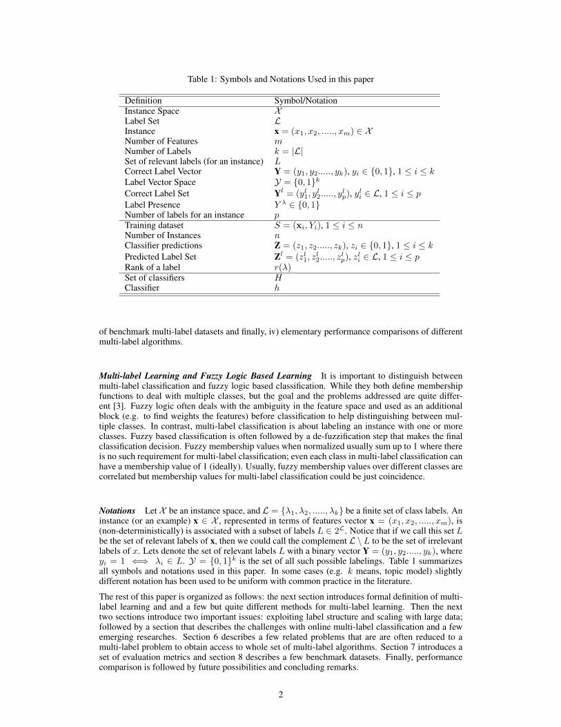
Table 1: Symbols and Notations Used in this paper

Definition Symbol/NotationInstance Space XLabel Set LInstance x = (x1, x2, ....., xm) ∈ XNumber of Features mNumber of Labels k = |L|Set of relevant labels (for an instance) LCorrect Label Vector Y = (y1, y2....., yk), yi ∈ {0, 1}, 1 ≤ i ≤ kLabel Vector Space Y = {0, 1}kCorrect Label Set Yl = (yl1, y

l2....., y

lp), yli ∈ L, 1 ≤ i ≤ p

Label Presence Y λ ∈ {0, 1}Number of labels for an instance pTraining dataset S = (xi, Yi), 1 ≤ i ≤ nNumber of Instances nClassifier predictions Z = (z1, z2....., zk), zi ∈ {0, 1}, 1 ≤ i ≤ kPredicted Label Set Zl = (zl1, z

l2....., z

lp), zli ∈ L, 1 ≤ i ≤ p

Rank of a label r(λ)Set of classifiers HClassifier h

of benchmark multi-label datasets and finally, iv) elementary performance comparisons of differentmulti-label algorithms.

Multi-label Learning and Fuzzy Logic Based Learning It is important to distinguish betweenmulti-label classification and fuzzy logic based classification. While they both define membershipfunctions to deal with multiple classes, but the goal and the problems addressed are quite differ-ent [3]. Fuzzy logic often deals with the ambiguity in the feature space and used as an additionalblock (e.g. to find weights the features) before classification to help distinguishing between mul-tiple classes. In contrast, multi-label classification is about labeling an instance with one or moreclasses. Fuzzy based classification is often followed by a de-fuzzification step that makes the finalclassification decision. Fuzzy membership values when normalized usually sum up to 1 where thereis no such requirement for multi-label classification; even each class in multi-label classification canhave a membership value of 1 (ideally). Usually, fuzzy membership values over different classes arecorrelated but membership values for multi-label classification could be just coincidence.

Notations Let X be an instance space, and L = {λ1, λ2, ....., λk} be a finite set of class labels. Aninstance (or an example) x ∈ X , represented in terms of features vector x = (x1, x2, ....., xm), is(non-deterministically) is associated with a subset of labels L ∈ 2L. Notice that if we call this set Lbe the set of relevant labels of x, then we could call the complement L \L to be the set of irrelevantlabels of x. Lets denote the set of relevant labels L with a binary vector Y = (y1, y2....., yk), whereyi = 1 ⇐⇒ λi ∈ L. Y = {0, 1}k is the set of all such possible labelings. Table 1 summarizesall symbols and notations used in this paper. In some cases (e.g. k means, topic model) slightlydifferent notation has been used to be uniform with common practice in the literature.

The rest of this paper is organized as follows: the next section introduces formal definition of multi-label learning and and a few but quite different methods for multi-label learning. Then the nexttwo sections introduce two important issues: exploiting label structure and scaling with large data;followed by a section that describes the challenges with online multi-label classification and a fewemerging researches. Section 6 describes a few related problems that are are often reduced to amulti-label problem to obtain access to whole set of multi-label algorithms. Section 7 introduces aset of evaluation metrics and section 8 describes a few benchmark datasets. Finally, performancecomparison is followed by future possibilities and concluding remarks.

2

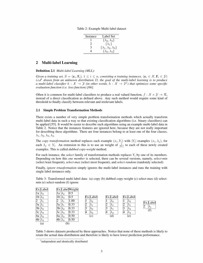
Table 2: Example Multi-label dataset

Instance Label Set1 {λ2, λ3}2 {λ1}3 {λ1, λ2, λ3}4 {λ2, λ4}

2 Multi-label Learning

Definition 2.1 Multi-label Learning (MLL):

Given a training set, S = (xi,Yi), 1 ≤ i ≤ n, consisting n training instances, (xi ∈ X ,Yi ∈ Y)i.i.d1 drawn from an unknown distribution D, the goal of the multi-label learning is to producea multi-label classifier h : X → Y (in other words, h : X → 2L) that optimizes some specificevaluation function (i.e. loss function) [66].

Often it is common for multi-label classifiers to produce a real valued function, f : X × Y → R,instead of a direct classification as defined above. Any such method would require some kind ofthreshold to finally classify between relevant and irrelevant labels.

2.1 Simple Problem Transformation Methods

There exists a number of very simple problem transformation methods which actually transformmulti-label data in such a way so that existing classification algorithms (i.e. binary classifiers) canbe applied [55]. It would be easier to describe such algorithms using an example multi-label data inTable 2. Notice that the instances features are ignored here, because they are not really importantfor describing these algorithms. There are four instances belong to at least one of the four classes,λ1, λ2, λ3, λ4.

The copy transformation method replaces each example (xi, Yi) with |Yi| examples (xi, λj), foreach λj ∈ Yi. An extension to this is to use an weight of 1

|Yi| to each of these newly createdexamples. This is called dubbed copy-weight method.

For each instance, the select family of transformation methods replaces Yi by one of its members.Depending on how this one member is selected, there can be several versions, namely, select-min(select least frequent), select-max (select most frequent), and select-random (randomly selected).

Finally, ignore trnasformation simply ignores the multi-label instances and runs the training withsingle label instances only.

Table 3: Transformed multi-label data: (a) copy (b) dubbed copy-weight (c) select-max (d) select-min (e) select-random (f) ignore

Ex.Label1a λ21b λ32 λ13a λ13b λ23c λ34a λ24b λ4

(a)

Ex.LabelWeight1a λ2 0.51b λ3 0.52 λ1 1.003a λ1 0.333b λ2 0.333c λ3 0.334a λ2 0.504b λ4 0.50

(b)

Ex.Label1 λ22 λ13 λ24 λ2

(c)

Ex.Label1 λ32 λ13 λ14 λ4

(d)

Ex.Label1 λ32 λ13 λ24 λ4

(e)

Ex.Label2 λ1

(f)

Table 3 shows datasets produced by these approaches. Notice that none of these methods is likely toretain the actual data distribution and therefore is likely to have lower prediction performance.

1independent and identically distributed

3

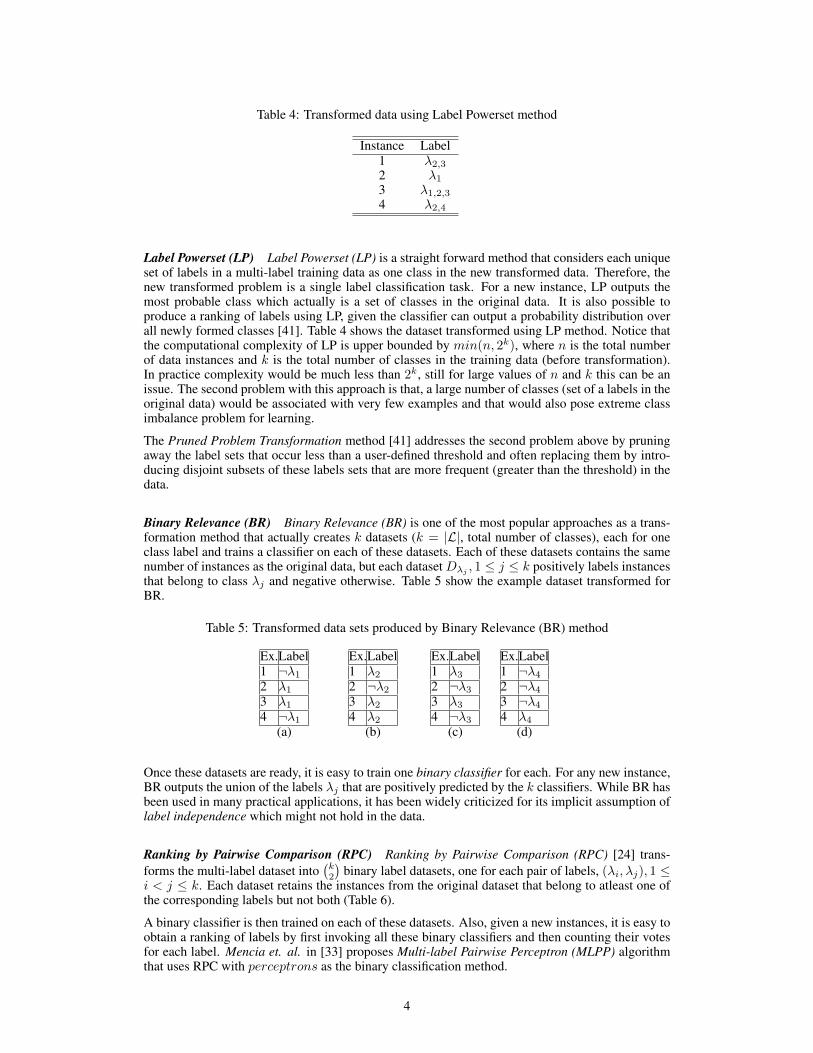
Table 4: Transformed data using Label Powerset method

Instance Label1 λ2,32 λ13 λ1,2,34 λ2,4

Label Powerset (LP) Label Powerset (LP) is a straight forward method that considers each uniqueset of labels in a multi-label training data as one class in the new transformed data. Therefore, thenew transformed problem is a single label classification task. For a new instance, LP outputs themost probable class which actually is a set of classes in the original data. It is also possible toproduce a ranking of labels using LP, given the classifier can output a probability distribution overall newly formed classes [41]. Table 4 shows the dataset transformed using LP method. Notice thatthe computational complexity of LP is upper bounded by min(n, 2k), where n is the total numberof data instances and k is the total number of classes in the training data (before transformation).In practice complexity would be much less than 2k, still for large values of n and k this can be anissue. The second problem with this approach is that, a large number of classes (set of a labels in theoriginal data) would be associated with very few examples and that would also pose extreme classimbalance problem for learning.

The Pruned Problem Transformation method [41] addresses the second problem above by pruningaway the label sets that occur less than a user-defined threshold and often replacing them by intro-ducing disjoint subsets of these labels sets that are more frequent (greater than the threshold) in thedata.

Binary Relevance (BR) Binary Relevance (BR) is one of the most popular approaches as a trans-formation method that actually creates k datasets (k = |L|, total number of classes), each for oneclass label and trains a classifier on each of these datasets. Each of these datasets contains the samenumber of instances as the original data, but each dataset Dλj , 1 ≤ j ≤ k positively labels instancesthat belong to class λj and negative otherwise. Table 5 show the example dataset transformed forBR.

Table 5: Transformed data sets produced by Binary Relevance (BR) method

Ex.Label1 ¬λ12 λ13 λ14 ¬λ1

(a)

Ex.Label1 λ22 ¬λ23 λ24 λ2

(b)

Ex.Label1 λ32 ¬λ33 λ34 ¬λ3

(c)

Ex.Label1 ¬λ42 ¬λ43 ¬λ44 λ4

(d)

Once these datasets are ready, it is easy to train one binary classifier for each. For any new instance,BR outputs the union of the labels λj that are positively predicted by the k classifiers. While BR hasbeen used in many practical applications, it has been widely criticized for its implicit assumption oflabel independence which might not hold in the data.

Ranking by Pairwise Comparison (RPC) Ranking by Pairwise Comparison (RPC) [24] trans-forms the multi-label dataset into

(k2

)binary label datasets, one for each pair of labels, (λi, λj), 1 ≤

i < j ≤ k. Each dataset retains the instances from the original dataset that belong to atleast one ofthe corresponding labels but not both (Table 6).

A binary classifier is then trained on each of these datasets. Also, given a new instances, it is easy toobtain a ranking of labels by first invoking all these binary classifiers and then counting their votesfor each label. Mencia et. al. in [33] proposes Multi-label Pairwise Perceptron (MLPP) algorithmthat uses RPC with perceptrons as the binary classification method.

4

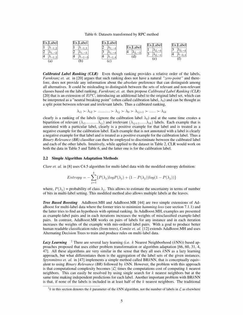
Table 6: Datasets transformed by RPC method

Ex.Label1 λ¬1,22 λ1,¬24 λ¬1,2

(a)

Ex.Label1 λ¬1,32 λ1,¬34 λ¬1¬3

(b)

Ex.Label2 λ1,¬43 λ1,¬44 λ¬1,4

(c)

Ex.Label4 λ2,¬3

(d)

Ex.Label1 λ2,¬43 λ2,¬4

(e)

Ex.Label3 λ3,¬44 λ¬3,4

(f)

Calibrated Label Ranking (CLR) Even though ranking provides a relative order of the labels,Furnkranz et. at. in [20] argues that such ranking does not have a natural ”zero-point” and there-fore, does not provide any information about the absolute preference that can distinguish amongall alternatives. It could be misleading to distinguish between the sets of relevant and non-relevantclasses based on the label ranking. Furnkranz et. at. then propose Calibrated Label Ranking (CLR)[20] that is an extension of RPC, introducing an additional label to the original label set, which canbe interpreted as a ”neutral breaking point” (often called calibration label, λ0) and can be thought asa split point between relevant and irrelevant labels. Thus a calibrated ranking,

λi1 � λi2 � ........... � λij � λ0 � λij+1 � ...... � λikclearly is a ranking of the labels (ignore the calibration label λ0) and at the same time creates abipartition of relevant (λi1...........λij) and irrelevant (λij+1......λik) labels. Each example that isannotated with a particular label, clearly is a positive example for that label and is treated as anegative example for the calibration label. Each example that is not annotated with a label is clearlya negative example for that label and is treated as a positive example for the calibration label. Thus aBinary Relevance (BR) classifier can then be employed to discriminate between the calibrated labeland each of the other labels. Intuitively, while applied to the dataset in Table 2, CLR would work onboth the data in Table 5 and Table 6, and the latter one is for the calibration label.

2.2 Simple Algorithm Adaptation Methods

Clare et. al. in [8] uses C4.5 algorithm for multi-label data with the modified entropy definition:

Entropy = −k∑j=1

{P (λj)logP (λj) + (1− P (λj))log(1− P (λj))}

where, P (λj) = probability of class λj . This allows to estimate the uncertainty in terms of numberof bits in multi-label setting. This modified method also allows multiple labels at the leaves.

Tree Based Boosting AdaBoost.MH and AdaBoost.MR [44] are two simple extensions of Ad-aBoost for multi-label data where the former tries to minimize hamming loss (see section 7.1.1) andthe latter tries to find an hypothesis with optimal ranking. In AdaBoost.MH, examples are presentedas example-label pairs and in each iterations increases the weights of misclassified example-labelpairs. In contrast, AdaBoost.MR works on pairs of labels for any instance and in each iterationincreases the weights of the example with mis-ordered label pairs. With a goal to produce betterhuman readable classification rules (from trees), Comite et. al. [12] extends AdaBoost.MH and usesAlternating Decision Trees to train and produce rules on multi-label data.

Lazy Learning 2 There are several lazy learning (i.e. k Nearest Neighborhood (kNN)) based ap-proaches proposed that uses either problem transformation or algorithm adaptation [66, 60, 31, 4,47]. All these algorithms are very similar in the sense that they all uses kNN as a lazy learningapproach, but what differentiates them is the aggregation of the label sets of the given instances.Spyromitros et. al. in [47] implements a simple method called BRkNN, that is conceptually equiv-alent to using Binary Relevance (BR) followed by kNN. However, the problem with this approachis that computational complexity becomes |L| times the computations cost of computing k nearestneighbors. This can easily be resolved by using single search for k nearest neighbors but at thesame time making independent predictions for each label. Another important problem with BRkNNis that, if none of the labels is included in at least half of the k nearest neighbors. The traditional

2k in this section denotes the k parameter of the kNN algorithm, not the number of labels in L as elsewhere

5

BRkNN is tempted to output an empty label set in that case. Spyromitros et. al. propose two ex-tensions to BRkNN, both based on confidence of each label, to solve this empty label set problem[47]. First, they argue that the proportion of data instances belonging to some class λ in k nearestneighbors of the test data instance is a good measure of confidence of the class label λ for that testinstance.

Confidence(λ) =1

k

k∑j=1

INj (λ)

where, N is the set of labels for k nearest neighbors and,

INj (λ) =

{1 if λ ∈ Nj0 otherwise

Therefore, in case of empty label set problem, they propose to return the label with highest confi-dence. The second extension they propose is to calculate the average size of of the label sets of the knearest neighbors (averagesize, s = 1

k

∑kj=1 |Nj |) and anytime output s (to nearest integer value)

highest confident labels for any test instance.

ML-kNN: This approach is also based onBR, but to find the label set for a given test instance it usesmaximum a posteriori (MAP) [13], based on prior and posterior probabilities of for each k nearestneighbor label. For each instance, ML-kNN first identifies its k nearest neighbors in the training setand then poses the problem as a MAP problem below:

Zλt = arg maxb∈{0,1}

P (Hλb |EλCt(λ)), l ∈ L

where, Zλt = predicted label set for instance t, Hλ1 (t) and Hλ

0 (t) be the events that t has label λ anddoes not have label λ respectively, Eλi is the event that exactly j instances of k nearest neighbor oftest instance t has label λ and, Ct(λ) is the membership vector that counts the number of neighborsof t belonging to class λ. This can be re-written as:

Zλt = arg maxb∈{0,1}

P (Hλb )P (EλCt(λ)|H

λb ), l ∈ L

and can be directly estimated from the training data.

Finally, Multi-class Multi-label Associative Classification (MMAC) [50] is an associative rule learn-ing based covering algorithm, that recursively learns a new rule and each time removes the examplesassociated with the rule. Labels for the test instance are ranked according to the support of the rulethat applies with the test instance. [57] extends this idea combined with lazy learning delaying theinductive process until a test instance arrives.

There also exists Neural Networks and Multi-layer perceptron based algorithms that has beenextended for multi-label data. In BP-MLL [65], the error function for the very common neuralnetwork learning algorithm, back-propagation has been modified to account for multi-label data.Multi-layer perceptron is easy to extend for multi-label data where one output node is maintainedfor each class label. A family of online algorithms for Multi-class Multi-layer Perceptron (MMP)has been proposed in [11] where the perceptron algorithms weight update is performed in such away so that it leads to correct label ranking.

Discriminative SVM Based Methods One important problem with tree based boosting [44] (dis-cussed in section 2.2) is that, they are likely to overfit with relatively smaller (< 1000) training set.Elisseeff et. al. in [18] propose an SVM algorithm that has an intuitive way of controlling suchcomplexity while having a small empirical error. Godbole et. al. present three improvements forBR with SVM to exploit label correlations that improves the margin [22]:

The first idea is to have an extended dataset with k (= |L|) additional features which are actually thepredictions of each binary classifier at the first round. The k new binary classifiers are trained on thisextended dataset. In this way the extended BR takes into account potential label dependencies. Thesecond idea, ConfMat, based on a confusion matrix, removes negative training examples of a com-plete label if it is very similar to the positive label. The third idea is called BandSVM, removes verysimilar negative examples that are within a threshold distance from the learned decision hyperplane,and this helps building better models especially in the presence of overlapping classes.

6

2.3 Dimensionality Reduction and Subspace Based Methods

In order to reduce the curse of dimensionality, features selection and extraction methods are verycommon in single label data. The wrapper based features selection [27] methods are equally appli-cable for multi-label data with a modified goal of reducing any multi-label loss function (see section7). An alternative could be to transform multi-label data into single label data (e.g. BR) and thenapply features selection to evaluate the discriminative power of each feature with respect to eachlabel. Any unsupervised method for dimensionality reduction such as, Principal Components Anal-ysis (PCA) and Latent Semantic Indexing (LSI) can also be used with multi-label data without anymodification. However, Yu et. al argue that even though such unsupervised algorithms can be useddirectly, if the relevant class label information is available, then taking that into account while deriv-ing the objective function should be beneficial [64]. Based on this idea, they propose a Multi-labelInformed Latent Semantic Indexing (MLSI) that preserves the feature information as well as capturesthe label correlations, while posing the LSI problem as an optimization problem.

On the other hand, supervised subspace based methods require modifications to be applicable tomulti-label data. A multi-label version of Linear Discriminant Analysis (LDA) has been proposedin [38] where the objective function, the ratio of inter-class distance to intra-class distance has beenadapted for multi-label data.

Shared Subspace Shared subspace based approaches assumes that there exist a common sub-space that is shared among the class labels. Therefore, any algorithm that intend to extract theshared subspace and the decision function is learnt on that subspace not only reduce the informa-tion redundancy but also is able to take into account the label correlations. Yan et. al. proposea boosting algorithm called Model-shared Subspace Boosting (MSSBoost) [62]. This method usesrandom subspace sampling to select feature subspace to work on and then, model sharing techniquesto automatically find, share and combine a number of random subspaces, and finally boosting basedensemble learning to jointly optimize the loss function over all labels. A much simpler method forthe same purpose is proposed in [25] that uses a linear transformation method to capture the sharedsubspace and finally uses a binary classifier train on this shared subspace.

2.4 Ensemble Methods3

The Random k labelsets (RAkEL) proposed by Tsoumakas et. al. [54] is an ensemble method thatiteratively constructs an ensemble of some (# of models desired, m) Label Powerset(LP) clasifiers.At each iteration it randomly selects (without replacement) k-labelset and learns and LP classifierand finally outputs all classifiers learnt. Notice,m and k are two important parameters, and the claimis that for small values of k and adequately large m, RAkEL is able to model label correlationseffectively. Notice, k = 1 and m = |L| would imply each time training an LP classifier andtherefore a total number for L classifiers are trained, one for each class; this is Binary Relevance(BR). Similarly, k = L and m = 1 would turn it into a single global LP classifier.

To address the class imbalance problem (very few instances in some classes) in LP Read et. al. in[42] proposes Pruned Sets method. The idea is based on pruning away infrequently occurring labelsets in LP , and this allows to focus only on most important label correlations, with reduced com-plexity. To compensate for such information loss, pruned away sets are broken into more frequentlyoccurring subsets and is introduced in the data again once crosses some predefined threshold. Anensemble of such pruned set classifiers is also proposed and for classification of a new instance avoting scheme is followed.

Zhang et. al. [69] present a Random Decision Tree (RDT) based ensemble and demonstrate thatthe training complexity is independent from the number of class labels. RDT constructs severaldecision tree randomly (i.e. picks a remaining feature randomly at each node) and stops growingonce it crosses some predefined threshold. Theoretical risk analysis of RDT shows that the upperbound of the risk is stable and lower bound decreases with the increase of number of trees [69].Importantly, increased number of trees in RDT guarantees improved performance with slightlyincreased complexity, though such increased complexity is better than most other methods. Thisidea of RDT can be used with both LP and BR and in both cases the computational complexity is

3k in this section is the parameter for RAkEL

7

free of number of labels. This property makes it better than the hierarchical model based algorithmHOMER [53] (see section 4), in terms of both performance and complexity.

2.5 Generative Modeling for Multi-label Data4

Several generative modeling based approach had been proposed [32, 56, 59] especially for model-ing the generative process of text based multi-label data. McCallum in [32] proposes a generativemodel for multi-labelled document that starts with selecting a set of classes (class labels for a doc-ument) with a mixture of weights for those classes. Next, each word in the document is generatedby first selecting a class according to the weight distribution and then the selected class is allowedto generate a word. Using the single apriori on most probable weight vector, ~Ψ~c, given the set ofclasses ~c, an approximate closed form generative process has been defined as:

P (~c|d) ≈ P (~c)∏w∈d

∑c∈C

~Ψ~ccP (w|c)

Finally, an Expectation Maximization(EM) [16] based parameter estimation method has been pro-posed for the above model. A similar word based parametric mixture models (PMM) has beenpresented in [56] that directly models the probability of each word appearing in each documentbelonging to some class.

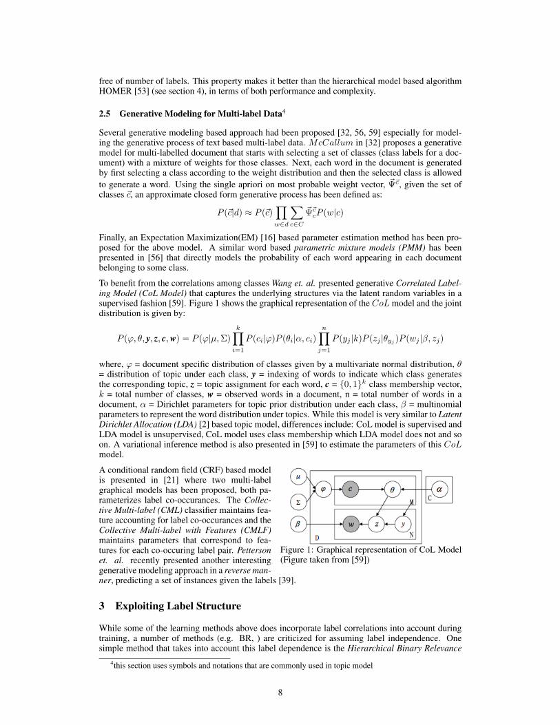
To benefit from the correlations among classes Wang et. al. presented generative Correlated Label-ing Model (CoL Model) that captures the underlying structures via the latent random variables in asupervised fashion [59]. Figure 1 shows the graphical representation of the CoLmodel and the jointdistribution is given by:

P (ϕ, θ, y, z, c,w) = P (ϕ|µ,Σ)

k∏i=1

P (ci|ϕ)P (θi|α, ci)n∏j=1

P (yj |k)P (zj |θyj )P (wj |β, zj)

where, ϕ = document specific distribution of classes given by a multivariate normal distribution, θ= distribution of topic under each class, y = indexing of words to indicate which class generatesthe corresponding topic, z = topic assignment for each word, c = {0, 1}k class membership vector,k = total number of classes, w = observed words in a document, n = total number of words in adocument, α = Dirichlet parameters for topic prior distribution under each class, β = multinomialparameters to represent the word distribution under topics. While this model is very similar to LatentDirichlet Allocation (LDA) [2] based topic model, differences include: CoL model is supervised andLDA model is unsupervised, CoL model uses class membership which LDA model does not and soon. A variational inference method is also presented in [59] to estimate the parameters of this CoLmodel.

Figure 1: Graphical representation of CoL Model(Figure taken from [59])

A conditional random field (CRF) based modelis presented in [21] where two multi-labelgraphical models has been proposed, both pa-rameterizes label co-occurances. The Collec-tive Multi-label (CML) classifier maintains fea-ture accounting for label co-occurances and theCollective Multi-label with Features (CMLF)maintains parameters that correspond to fea-tures for each co-occuring label pair. Pettersonet. al. recently presented another interestinggenerative modeling approach in a reverse man-ner, predicting a set of instances given the labels [39].

3 Exploiting Label Structure

While some of the learning methods above does incorporate label correlations into account duringtraining, a number of methods (e.g. BR, ) are criticized for assuming label independence. Onesimple method that takes into account this label dependence is the Hierarchical Binary Relevance

4this section uses symbols and notations that are commonly used in topic model

8

(HBR) (given a hierarchy, traing a binary classifier for each non-root class) method, where an im-plicit constraint is that an instance cannot belong to a class if it is not associated with its parent.Similar hierarchical approach has been utilized in all tree based methods (e.g. Tree Based Boost-ing, HOMER etc.). All these methods are capable of utilizing label dependencies reflected in theirimproved predictive accuracies.

However, it is important to note that there exists two different kinds of label dependence: condi-tional and unconditional, and substantially different approaches are needed to exploit these differentdependencies [15]. Zhu et. al. in [71] present a maximum entropy based method that explicitlymodels the mutual correlations among the classes by constructing a conditional probability modelfrom the training data. Unlike other traditional approaches, the conditional probability model pa-rameters here are estimated through maximum entropy method subject to the prior probabilities ofeach category (i. e. Ee(λ) = Em(λ) + η,E = expectation, e = empirical,m =model distri-bution, η = error) and correlations among the categories and the features of the given data (i. e.Ee(λ|xj) = Em(λ|xj) + φ), and Ee(λiλj) = Em(λiλj) + θij , φ = error, θij = error) and fi-nally, solved using Lagrangian. A similar approach is presented in [67] that uses Bayesian Networkto encode the label dependencies.

To estimate the joint distribution of labels a completely different idea proposed in [14] is to learn kdifferent function (k = |L|) on extended input space X × {0, 1}i−1, where predictions for classes,y1, y2, ......, yi−1 (notice that this idea is very similar the SVM based approach presented in 2.2) areconsidered as additional features.

fi : X × {0, 1}i−1 → [0, 1]

(x, y1, y2, ....., yi−1)→ P (yi = 1|x, y1, y2, ....., yi−1)

where, fi can be interpreted as a probabilistic classifier and this approach is called proba-bilistic classifier chain (PCC). The idea is further extended to construct an ensemble, calledprobabilistic classifier chain (EPCC).

Encoding in Input Space A completely different approach called the Instance Differentiation(INSDIF) [68] is based on the idea that multi-label learning can be better efficient if the input spaceinherent ambiguity can be expressed explicitly. The two stage algorithm first computes a prototypevector for each class by averaging all instances belonging to that class and then each instance isrepresented by a bag of instances, that are the differences between the instance itself and each ofthe prototype vectors. The second step is to use a two level classification strategy: using k-medoidsalgorithm to find a fixed number of clusters representing the underlying structure of the data andthen finding a discriminative linear classifier weights based on the features computed by using thedistance between the bag of instances and the cluster medoids (notice that the second step is similarto solving Multi-Instance Multi-label problem discussed in section 6.3).

4 Scaling with Large Data

Often a number of domains and applications require multi-label algorithms to scale up with largedata such as delicious, EUROVOC (see section 8.2), and the problem space could be nearly un-bounded if we consider the categorization of the web. Such large domains pose a few challenges tothe existing algorithms, especially because the label space is also likely to grow with the exponentialgrowth of instance space. First, with a large label space, number of training examples labeled fora particular class will be significantly less compared to the total number of examples. Second, thecomputational cost of training a multi-label classifier is usually strongly affected by the number oflabels. This is true for most of the existing algorithms except for a few such as binary relevancewhose complexity is linear with respect to |L|, but usually criticized for label independence as-sumption. Finally, most of the methods need to maintain a large number of models in memory and,therefore, may fail to scale with large label space.

Most of the existing algorithms described above either do not scale or result in unsatisfactoryperformance. Tang et. al. in [49] present a MetaLabeler approach that first constructs ameta dataset where each data instance is a function of corresponding instance in the originaldataset. Three different such function has been proposed: content-based (φ(x) = x), score-based (φ(x) = [f1(x), ......, fk(x)], fi(x) = prediction score for class λi) and, rank-based (φ(x) =

9

ψ(f1(x), ....., fk(x)), ψ(x) = a vector of sorted scores). One-vs-rest SVM model is trained on thismeta dataset and finally, the class labels are selected based on their scores.

Dekel et. al. propose a pruning based two step method, which is very similar to the ensemble prunedset method discussed above (see section 2.4). Theoretically and experimentally they have shown thatthis method is capable of dealing very sparse situation even with more classes than instances [36].In the learning step, any arbitrary classifier, h is trained on the training data. In the post learningstep, the goal is to find a label transformation function, φ so that the final classifier is the compositeof the two, φ ◦ h. This label transformation in this case is defined as a set of label pruning rulesthat minimizes the overall risk of φ ◦ h. A theoretical analysis of final empirical risk, Rφ and thefinal risk, Rφ shows that a simple pruning rule as, ‘pruning any label for which the ratio of falsepositive to true positive exceeds some threshold’, reduces the overall risk under mild conditions.More importantly, unlike most other methods, this method allow number of labels, k to grow asa function of number of instances, n. While this method seem to work competitively good evenwith large domain, Wikipedia, with 2.9 million articles and almost 1.5 million categories, a potentialcriticism against this method is the implicit label independence assumption. Also, incorporatingmore complicated pruning rules in the system is left as a future research question.

Hierarchical Methods The idea behind hierarchical model comes from the goal to reduce thecomputational complexity at each level and thus making the learning algorithm efficient especiallywith many labels. While the tree based boosting (see section 2.2) and random decision tree (seesection 2.4) based methods are very similar to the hierarchical method HOMER proposed in [53],what distinguishes HOMER from other methods is the balanced clustering [1] to explicitly maintainan even distribution of a set of labels into disjoint subsets so that similar labels are placed togetherand dissimilar apart. HOMER starts with all the labels (and instances) at the root and recursivelycreates an hierarchy in a top-down depth first fashion. At each node, b children nodes (b = userdefined branching factor) are created and the labels of the current node are distributed into b disjointsubsets, one for each child. Such distribution of labels among the children is performed using abalanced clustering method. They propose a Balanced k means algorithm which is an extensionof popular k means algorithm with an explicit constraint on the size of each cluster. Using suchbalanced label clusters would ensure reduced operational cost in terms of number of nodes to beactivated for any prediction. Once the balanced distribution of labels is done, a multi-label classifieris trained for the prediction of the meta-labels (disjunction of the labels at any node) of the childrenat current node.

5 Online Multi-label Learning

Many real world multi-label applications such as web text categorization, content based image orvideo annotation etc., require not only dealing with large volume of data but also demand for pro-cessing or update of the learning algorithm in an online fashion [61]. Unfortunately, most of thealgorithms described above does not scale well with large data and more importantly are not reallyapplicable for online learning. To address this issue, Hua et. al. propose a scalable framework forannotation based video search that relies on on an online multi-label active learning (Online MLAL)[23]. Online MLAL has three major modules: multi-label active learning, online multi-label learn-ing, and new label learning from zero knowledge. The first one is a simple active learning modulethat selects the most informative instance-label pair (x∗s, λ

∗s) to reduce the uncertainty along both

instance and label dimensionalities, based on Bayesian classification error over a sample of all in-stances. The assumption for Online MLAL is that the data is increasing batch by batch and onceand an initial classifier is build on the first batch, it can be updated through active learning oversucceeding batches. The goal for the second module is to make this algorithm run online with twospecific requirements: the classifier state does not change much from its current state, and revealsthe information contained in the newly arrived instances. The first one can be measured in terms ofKullback Leibler Divergence (KLD) [9] while ensuring the second one in terms of reducing bayesianerror; thus can be posed as an optimization problem subject to constraints. Finally, such classifica-tion scheme is extended to handle new labels (can be proposed from the query logs, if accessible)assuming the new labels are uniformly distributed.

In [61] Zhang et. al. present Bayesian Online Multi-label (BOMC) classification framework thatuses a probabilistic linear discriminant wc for each class c where {wc}c∈C are independent diagonal

10

Gaussians, whose mean and variance are estimated from the training data. The key model here isthe likelihood P (y|{wc}c, x) that is modeled using a factor graph. Also the posterior P ({wc}|y, x)can be estimated by marginalizing over different nodes (inner product nodes, noise additive nodesand the difference nodes) in the factor graph (for details see [61]). At each iteration, it takes oneadditional instance (xi, yi) and using a Gaussian prior P0(w), computes the posterior:

Pi(w|xi, yi) ∝ Pi−1(w)P (yi|w, xi)

This can actually be approximated by a Gaussian that is closest in terms of KL-divergence (KLD).Finally, such marginalization in subsequent nodes can be effectively performed by Expectation Prop-agation (EP) [35] through the factor graph.

6 Problem Variations

It is worth mentioning that the most popular single label multi-class classification (often the termsingle label is ignored) is a simple variation of multi-label classification problem, where the con-straint is that every instance can belong to only one class. That reduces the problem to learn aclassifier, hmulti−class : X → L. In this section, we describe a few more interesting problems thatclosely relates to multi-label problem.

6.1 Learning with Multiple Labels: Disjoint Case

Consider an example scenario where several human experts are hired to label some data into differentcategories. While we expect that they would agree in most (if not all) of the labels, they mightdisagree is some of the instances’ labels (e.g. consider a complicated labeling such as labelingemotions from image/video). This might result in multiple class labels for some instances whileonly one of them is actually correct. This problem is similar to traditional multi-label problembecause it also allows multiple labels for each instance, however, quite different because only oneof those labels (for an instance) is correct while in case of multi-label, all the labels are correct [26].

Definition 6.1 Learning with Multiple Labels (Disjoint Case): Let xi be an instance, Yi be the setof candidate class labels for xi. Assuming that model with parameter space Θ exists (that mapsinputs to correct output labels), the goal for learning from multiple label data (disjoint case) is toestimate θ ∈ Θ so that the predicted class zli for data instance xi is highly likely to be in Yi.

θ∗ = arg maxθ

∏i

P (zli ∈ Yl|xi, θ)

Notice that this problem is very similar to semi-supervised learning. Like semi-supervised learningthis problem has a portion of the data correctly labeled (labeled with only one class). But the rest ofthe data in case of semi-supervised learning is unlabeled and, therefore, the label search space is L(set of all labels) for those instances; whereas, in this case the search space is restricted to the givenlabels for those instances.

Finally, Jin et. al. in [26] proposes a discriminative Expectation Maximization (EM) [16] basedalgorithm to estimate θ∗, with and without prior assumption.

6.2 Multitask Learning

In machine learning, it is often common to break down a large problem in to a set of small and rea-sonably independent subproblems, learn them separately and them combine [5]. A counter argumentfor this approach is that this method ignores a lot of information and possible dependence among thesubproblems. For example, if we train a system to learn textures in isolation, that might fail in realscenario when tested with complex real-life scenes. In contrast, a system trained simultaneously ontextures, shades, shapes, reflections, shadows, orientations, edges, etc. can potentially benefit frominter-dependence among all these and is expected to perform better to recognize complex objectsin the real world. Intuitively, this approach is called multitask learning where the basic idea is that,if several tasks are related, then learning them simultaneously can improve the overall performancecompared to learning each of them separately [40].

11

Definition 6.2 Multitask Learning (MLT): Let Xi = (xi1, xi2....., ximi) ⊆ Xi be a set of instancesin the instance space Xi, Yli = (yli1, y

li2....., y

lipi

), ylij ⊆ Li, is a set of labelsets for each instancespace i, 1 ≤ i ≤ v, v = total number of spaces (different tasks), mi = total number of instances inspace i, pi = total number of different labels in space i. Now, if learning a task is actually to learna function from the input space X to the output space Yl, then multitask learning is the problem oflearning several functions fi : Xi → Yli.

The assumption here is, that the observations are disjoint but they are drawn from the same domain,i.e. X1 = X2 = ....... = Xv = X . It is also common to assume that the set of labels Yli aresame across all tasks, or we have access to some oracle that maps among labels in different spaces.One practical example5, is the problem of learning to automatically categorize objects on the web into an ontology or directory structure. Two most common applications for this problem are Yahoo!directory6 and DMOZ 7. Clearly, these two tasks are related, but they might differ in their labelsets. Having access to an oracle for mapping among label sets might not be a practical assumptionhere, still, learning the two problems simultaneously can greatly be benefitted by learning themsimultaneously.

There exists several methods in literature to address this problem of learning multiple tasks simul-taneously [30, 10]. Mencia in [30] argues that it would advantageous to consider all the parallelsubproblems as a single large problem and poses it as a multi-label problem, assuming that there isa common training set for all tasks.

6.3 Multi-Instance Multi-Label Learning (MIML)

In multi-instance multi-label problem, instances are organized into ’bags’ that may contain multipleinstances and the class label is assigned for each bag instead of each instance. The only constrainfor labeling each bag is that it needs to have at least one instance belonging to that class and the restcould be noise for that class. It is important to note that for multi-label problems, the ambiguity lieson the class label, but for multi-instance the ambiguity lies on the instances side [26]. This makesmulti-instance multi-label problems more difficult as they can have ambiguity in both sides.

Definition 6.3 Multi-instance Multi-label Learning (MIML): Let X be the instance space and L bethe set of labels. Given a dataset {(X1, Y

l1 ), (X2, Y

l2 ), ......, (Xn, Y

ln)} where Xi ⊆ X is a set of

instances {xi1, xi2, ....., xini}, xij ∈ X , 1 ≤ i ≤ n, 1 ≤ j ≤ ni, and Y li ⊆ L is a set of labels{yli1, yli2, ....., ylili}, y

lik ∈ L, 1 ≤ k ≤ li, where ni denotes the number of instances in Xi and li

denotes the number of labels in Y li .

If each Y li contains only one label (Y li = {yli}), then data is called multi-instance data and learn-ing a function fMIL : 2X → L

(in other words 2X × L → {+1,−1}

)is called multi-instance

learning.

Learning a function fMIML : 2X → 2L is called multi-instance multi-label learning8.

There are two common approaches to solve MIML problems [70]:

Using Multi-instance Learning: For any y ∈ L, fMIL(Xi, y) = +1 if y ∈ Y li and -1 oth-erwise. Now the appropriate label for a new instances X* can be computed as, Y* = {y|y ∈L and fMIL((X∗, y)) = +1}. Thus, we can transform fMIML : 2X → 2L into fMIL :2X × L → {+1,−1}.Using Multi-label Learning: Let φ is a function such that πi = φ(Xi), φ : 2X → Π. Now,for πi ∈ Π we can learn a multi-label algorithms such that, fMLL(πi) = fMIML(Xi), where,fMLL : Π→ 2|L|. Thus, we can transform fMIML : 2X → 2L into fMLL : Π→ 2|L|.

5example borrowed from [40]6http://dir.yahoo.com/7http://www.dmoz.org/8notice we have already defined multi-label learning in definition 2.1

12

7 Evaluation Metrices

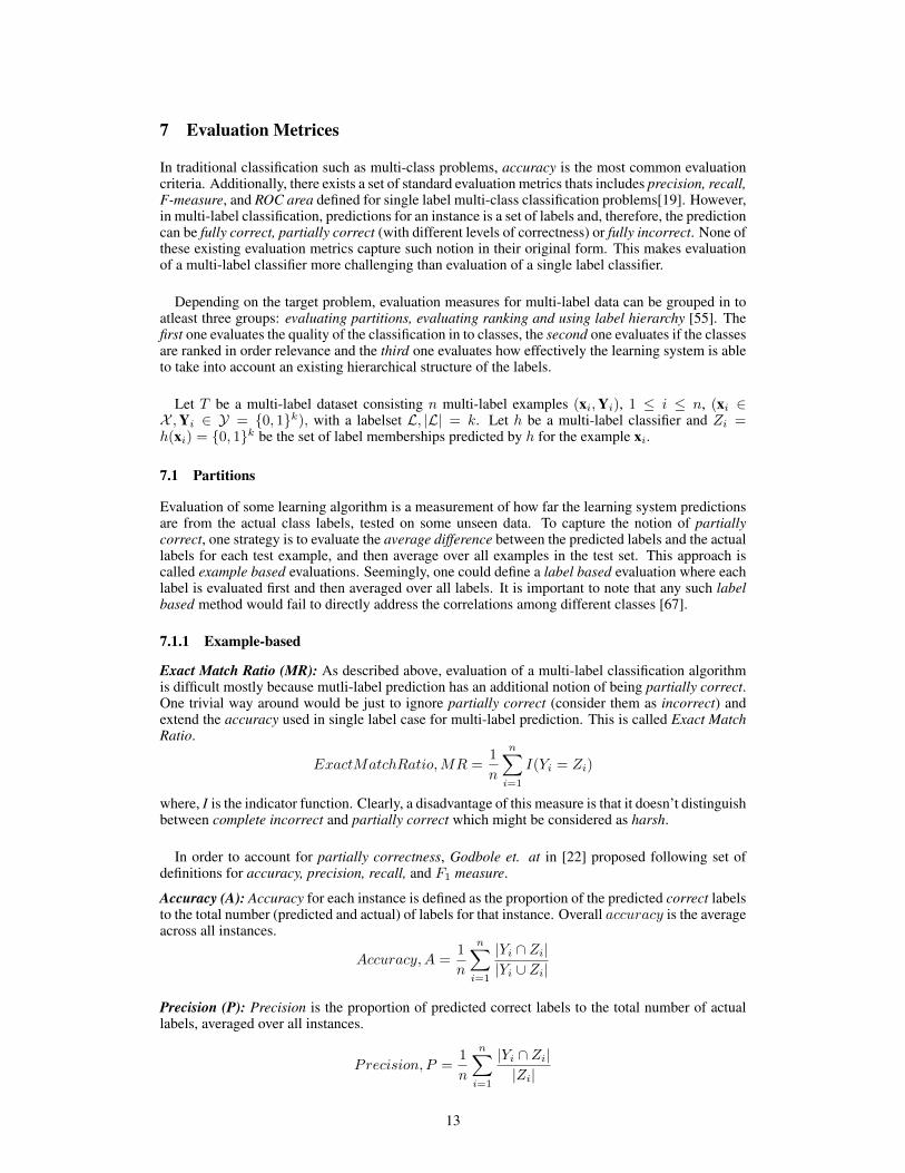
In traditional classification such as multi-class problems, accuracy is the most common evaluationcriteria. Additionally, there exists a set of standard evaluation metrics thats includes precision, recall,F-measure, and ROC area defined for single label multi-class classification problems[19]. However,in multi-label classification, predictions for an instance is a set of labels and, therefore, the predictioncan be fully correct, partially correct (with different levels of correctness) or fully incorrect. None ofthese existing evaluation metrics capture such notion in their original form. This makes evaluationof a multi-label classifier more challenging than evaluation of a single label classifier.

Depending on the target problem, evaluation measures for multi-label data can be grouped in toatleast three groups: evaluating partitions, evaluating ranking and using label hierarchy [55]. Thefirst one evaluates the quality of the classification in to classes, the second one evaluates if the classesare ranked in order relevance and the third one evaluates how effectively the learning system is ableto take into account an existing hierarchical structure of the labels.

Let T be a multi-label dataset consisting n multi-label examples (xi,Yi), 1 ≤ i ≤ n, (xi ∈X ,Yi ∈ Y = {0, 1}k), with a labelset L, |L| = k. Let h be a multi-label classifier and Zi =h(xi) = {0, 1}k be the set of label memberships predicted by h for the example xi.

7.1 Partitions

Evaluation of some learning algorithm is a measurement of how far the learning system predictionsare from the actual class labels, tested on some unseen data. To capture the notion of partiallycorrect, one strategy is to evaluate the average difference between the predicted labels and the actuallabels for each test example, and then average over all examples in the test set. This approach iscalled example based evaluations. Seemingly, one could define a label based evaluation where eachlabel is evaluated first and then averaged over all labels. It is important to note that any such labelbased method would fail to directly address the correlations among different classes [67].

7.1.1 Example-based

Exact Match Ratio (MR): As described above, evaluation of a multi-label classification algorithmis difficult mostly because mutli-label prediction has an additional notion of being partially correct.One trivial way around would be just to ignore partially correct (consider them as incorrect) andextend the accuracy used in single label case for multi-label prediction. This is called Exact MatchRatio.

ExactMatchRatio,MR =1

n

n∑i=1

I(Yi = Zi)

where, I is the indicator function. Clearly, a disadvantage of this measure is that it doesn’t distinguishbetween complete incorrect and partially correct which might be considered as harsh.

In order to account for partially correctness, Godbole et. at in [22] proposed following set ofdefinitions for accuracy, precision, recall, and F1 measure.

Accuracy (A): Accuracy for each instance is defined as the proportion of the predicted correct labelsto the total number (predicted and actual) of labels for that instance. Overall accuracy is the averageacross all instances.

Accuracy,A =1

n

n∑i=1

|Yi ∩ Zi||Yi ∪ Zi|

Precision (P): Precision is the proportion of predicted correct labels to the total number of actuallabels, averaged over all instances.

Precision, P =1

n

n∑i=1

|Yi ∩ Zi||Zi|

13

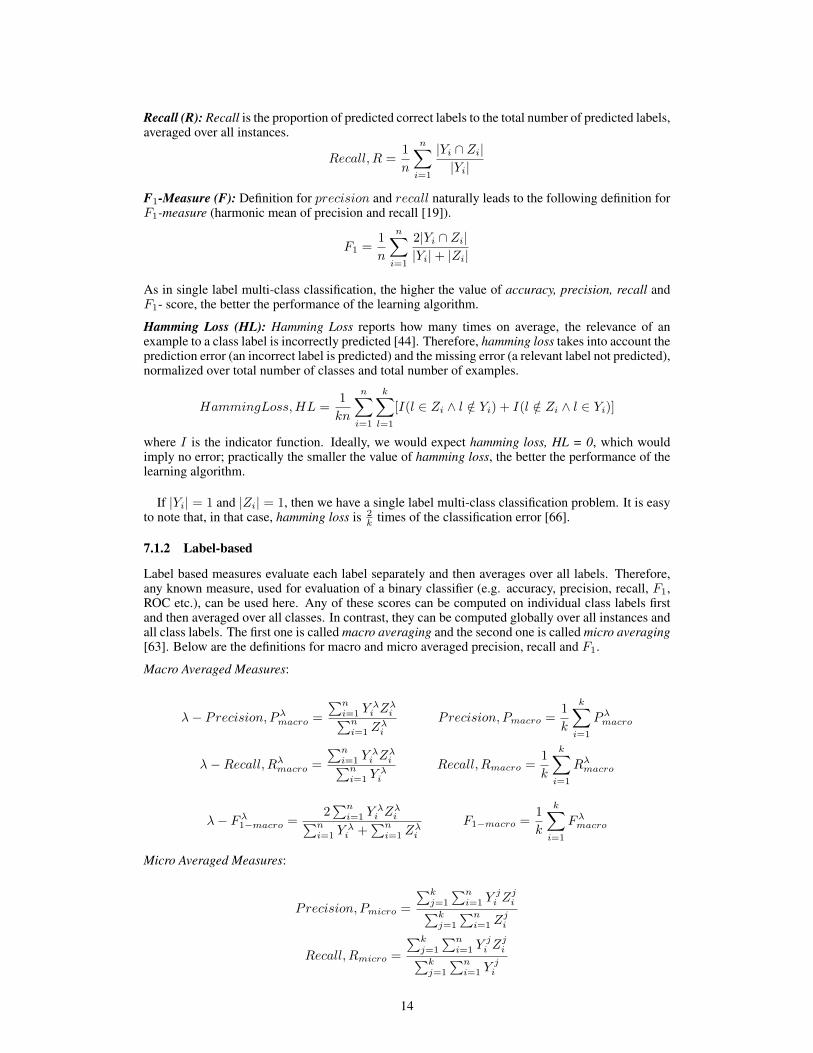
Recall (R): Recall is the proportion of predicted correct labels to the total number of predicted labels,averaged over all instances.

Recall, R =1

n

n∑i=1

|Yi ∩ Zi||Yi|

F1-Measure (F): Definition for precision and recall naturally leads to the following definition forF1-measure (harmonic mean of precision and recall [19]).

F1 =1

n

n∑i=1

2|Yi ∩ Zi||Yi|+ |Zi|

As in single label multi-class classification, the higher the value of accuracy, precision, recall andF1- score, the better the performance of the learning algorithm.

Hamming Loss (HL): Hamming Loss reports how many times on average, the relevance of anexample to a class label is incorrectly predicted [44]. Therefore, hamming loss takes into account theprediction error (an incorrect label is predicted) and the missing error (a relevant label not predicted),normalized over total number of classes and total number of examples.

HammingLoss,HL =1

kn

n∑i=1

k∑l=1

[I(l ∈ Zi ∧ l /∈ Yi) + I(l /∈ Zi ∧ l ∈ Yi)]

where I is the indicator function. Ideally, we would expect hamming loss, HL = 0, which wouldimply no error; practically the smaller the value of hamming loss, the better the performance of thelearning algorithm.

If |Yi| = 1 and |Zi| = 1, then we have a single label multi-class classification problem. It is easyto note that, in that case, hamming loss is 2

k times of the classification error [66].

7.1.2 Label-based

Label based measures evaluate each label separately and then averages over all labels. Therefore,any known measure, used for evaluation of a binary classifier (e.g. accuracy, precision, recall, F1,ROC etc.), can be used here. Any of these scores can be computed on individual class labels firstand then averaged over all classes. In contrast, they can be computed globally over all instances andall class labels. The first one is called macro averaging and the second one is called micro averaging[63]. Below are the definitions for macro and micro averaged precision, recall and F1.

Macro Averaged Measures:

λ− Precision, Pλmacro =

∑ni=1 Y

λi Z

λi∑n

i=1 Zλi

Precision, Pmacro =1

k

k∑i=1

Pλmacro

λ−Recall, Rλmacro =

∑ni=1 Y

λi Z

λi∑n

i=1 Yλi

Recall, Rmacro =1

k

k∑i=1

Rλmacro

λ− Fλ1−macro =2∑ni=1 Y

λi Z

λi∑n

i=1 Yλi +

∑ni=1 Z

λi

F1−macro =1

k

k∑i=1

Fλmacro

Micro Averaged Measures:

Precision, Pmicro =

∑kj=1

∑ni=1 Y

ji Z

ji∑k

j=1

∑ni=1 Z

ji

Recall, Rmicro =

∑kj=1

∑ni=1 Y

ji Z

ji∑k

j=1

∑ni=1 Y

ji

14

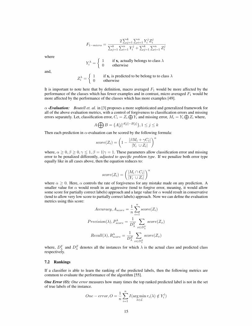
F1−micro =2∑kj=1

∑ni=1 Y

ji Z

ji∑k

j=1

∑ni=1 Y

ji +

∑kj=1

∑ni=1 Z

ji

where

Y λi =

{1 if xi actually belongs to class λ0 otherwise

and,

Zλi =

{1 if xi is predicted to be belong to to class λ0 otherwise

It is important to note here that by definition, macro averaged F1 would be more affected by theperformance of the classes which has fewer examples and in contrast, micro averaged F1 would bemore affected by the performance of the classes which has more examples [49].

α -Evaluation: Boutell et. al. in [3] proposes a more sophisticated and generalized framework forall of the above evaluation metrics, with a control of forgiveness to classification errors and missingerrors separately. Let, classification error, Ci = Zi

⊕Yi and missing error, Mi = Yi

⊕Zi where,

A⊕

B = {A[j]A[j]−B[j]}, 1 ≤ j ≤ k

Then each prediction in α-evaluation can be scored by the following formula:

score(Zi) =

(1− |βMi + γCi|

|Yi ∪ Zi|

)αwhere, α ≥ 0, β ≥ 0, γ ≤ 1, β = 1|γ = 1. These parameters allow classification error and missingerror to be penalized differently, adjusted to specific problem type. If we penalize both error typeequally like in all cases above, then the equation reduces to:

score(Zi) =

(|Mi ∩ Ci||Yi ∪ Zi|

)αwhere α ≥ 0. Here, α controls the rate of forgiveness for any mistake made on any prediction. Asmaller value for α would result in an aggressive (tend to forgive error, meaning, it would allowsome score for partially correct labels) approach and a large value for α would result in conservative(tend to allow very low score to partially correct labels) approach. Now we can define the evaluationmetrics using this score:

Accuracy,Ascore =1

n

n∑i=1

score(Zi)

Precision(λ), Pλscore =1

DYλ

∑x∈DYλ

score(Zx)

Recall(λ), Rλscore =1

DZλ

∑x∈DZλ

score(Zx)

where, DYλ and DZ

λ denotes all the instances for which λ is the actual class and predicted classrespectively.

7.2 Rankings

If a classifier is able to learn the ranking of the predicted labels, then the following metrics arecommon to evaluate the performance of the algorithm [55].

One Error (O): One error measures how many times the top ranked predicted label is not in the setof true labels of the instance.

One− error,O =1

n

n∑i=1

I(arg minλ∈L

ri(λ) /∈ Y li )

15

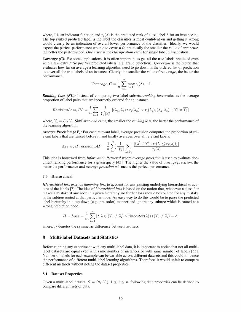
where, I is an indicator function and ri(λ) is the predicted rank of class label λ for an instance xi.The top ranked predicted label is the label the classifier is most confident on and getting it wrongwould clearly be an indication of overall lower performance of the classifier. Ideally, we wouldexpect the perfect performance when one error = 0; practically the smaller the value of one error,the better the performance. One error is the classification error for single label classification.

Coverage (C): For some applications, it is often important to get all the true labels predicted evenwith a few extra false positive predicted labels (e.g. fraud detection). Coverage is the metric thatevaluates how far on average a learning algorithm need to go down in the ordered list of predictionto cover all the true labels of an instance. Clearly, the smaller the value of coverage, the better theperformance.

Coverage, C =1

n

n∑i=1

maxλ∈Yi

ri(λ)− 1

Ranking Loss (RL): Instead of comparing two label subsets, ranking loss evaluates the averageproportion of label pairs that are incorrectly ordered for an instance.

RankingLoss,RL =1

n

n∑i=1

1

|Y li |Y li ||(λa, λb) : ri(λa) > ri(λb), (λa, λb) ∈ Y li × Y li |

where, Yi = L \ Yi. Similar to one error, the smaller the ranking loss, the better the performance ofthe learning algorithm.

Average Precision (AP): For each relevant label, average precision computes the proportion of rel-evant labels that are ranked before it, and finally averages over all relevant labels.

AveragePrecision,AP =1

n

n∑i=1

1

|Y li |∑λ∈Y li

|{λ′ ∈ Y li : ri(λ′ ≤ ri(λ))}|

ri(λ)

This idea is borrowed from Information Retrieval where average precision is used to evaluate doc-ument ranking performance for a given query [43]. The higher the value of average precision, thebetter the performance and average precision = 1 means the perfect performance.

7.3 Hierarchical

HIerarchical loss extends hamming loss to account for any existing underlying hierarchical strucu-ture of the labels [7]. The idea of hierarchical loss is based on the notion that, whenever a classifiermakes a mistake at any node in a given hierarchy, no further loss should be counted for any mistakein the subtree rooted at that particular node. An easy way to do this would be to parse the predictedlabel hierarchy in a top down (e.g. pre-order) manner and ignore any subtree which is rooted at awrong prediction node.

H − Loss =1

m

n∑i=1

|λ|λ ∈ (Yi ./ Zi) ∧Ancestor(λ) ∩ (Yi ./ Zi) = φ|

where, ./ denotes the symmetric difference between two sets.

8 Multi-label Datasets and Statistics

Before running any experiment with any multi-label data, it is important to notice that not all multi-label datasets are equal even with same number of instances or with same number of labels [55].Number of labels for each example can be variable across different datasets and this could influencethe performance of different multi-label learning algorithms. Therefore, it would unfair to comparedifferent methods without noting the dataset properties.

8.1 Dataset Properties

Given a multi-label dataset, S = (xi, Yi), 1 ≤ i ≤ n, following data properties can be defined tocompare different sets of data.

16

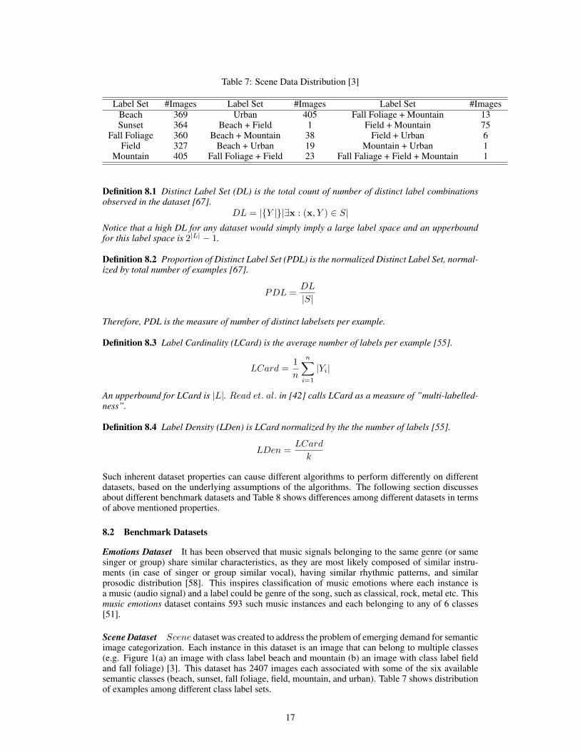
Table 7: Scene Data Distribution [3]

Label Set #Images Label Set #Images Label Set #ImagesBeach 369 Urban 405 Fall Foliage + Mountain 13Sunset 364 Beach + Field 1 Field + Mountain 75

Fall Foliage 360 Beach + Mountain 38 Field + Urban 6Field 327 Beach + Urban 19 Mountain + Urban 1

Mountain 405 Fall Foliage + Field 23 Fall Faliage + Field + Mountain 1

Definition 8.1 Distinct Label Set (DL) is the total count of number of distinct label combinationsobserved in the dataset [67].

DL = |{Y |}|∃x : (x, Y ) ∈ S|Notice that a high DL for any dataset would simply imply a large label space and an upperboundfor this label space is 2|L| − 1.

Definition 8.2 Proportion of Distinct Label Set (PDL) is the normalized Distinct Label Set, normal-ized by total number of examples [67].

PDL =DL

|S|

Therefore, PDL is the measure of number of distinct labelsets per example.

Definition 8.3 Label Cardinality (LCard) is the average number of labels per example [55].

LCard =1

n

n∑i=1

|Yi|

An upperbound for LCard is |L|. Read et. al. in [42] calls LCard as a measure of ”multi-labelled-ness”.

Definition 8.4 Label Density (LDen) is LCard normalized by the the number of labels [55].

LDen =LCard

k

Such inherent dataset properties can cause different algorithms to perform differently on differentdatasets, based on the underlying assumptions of the algorithms. The following section discussesabout different benchmark datasets and Table 8 shows differences among different datasets in termsof above mentioned properties.

8.2 Benchmark Datasets

Emotions Dataset It has been observed that music signals belonging to the same genre (or samesinger or group) share similar characteristics, as they are most likely composed of similar instru-ments (in case of singer or group similar vocal), having similar rhythmic patterns, and similarprosodic distribution [58]. This inspires classification of music emotions where each instance isa music (audio signal) and a label could be genre of the song, such as classical, rock, metal etc. Thismusic emotions dataset contains 593 such music instances and each belonging to any of 6 classes[51].

Scene Dataset Scene dataset was created to address the problem of emerging demand for semanticimage categorization. Each instance in this dataset is an image that can belong to multiple classes(e.g. Figure 1(a) an image with class label beach and mountain (b) an image with class label fieldand fall foliage) [3]. This dataset has 2407 images each associated with some of the six availablesemantic classes (beach, sunset, fall foliage, field, mountain, and urban). Table 7 shows distributionof examples among different class label sets.

17

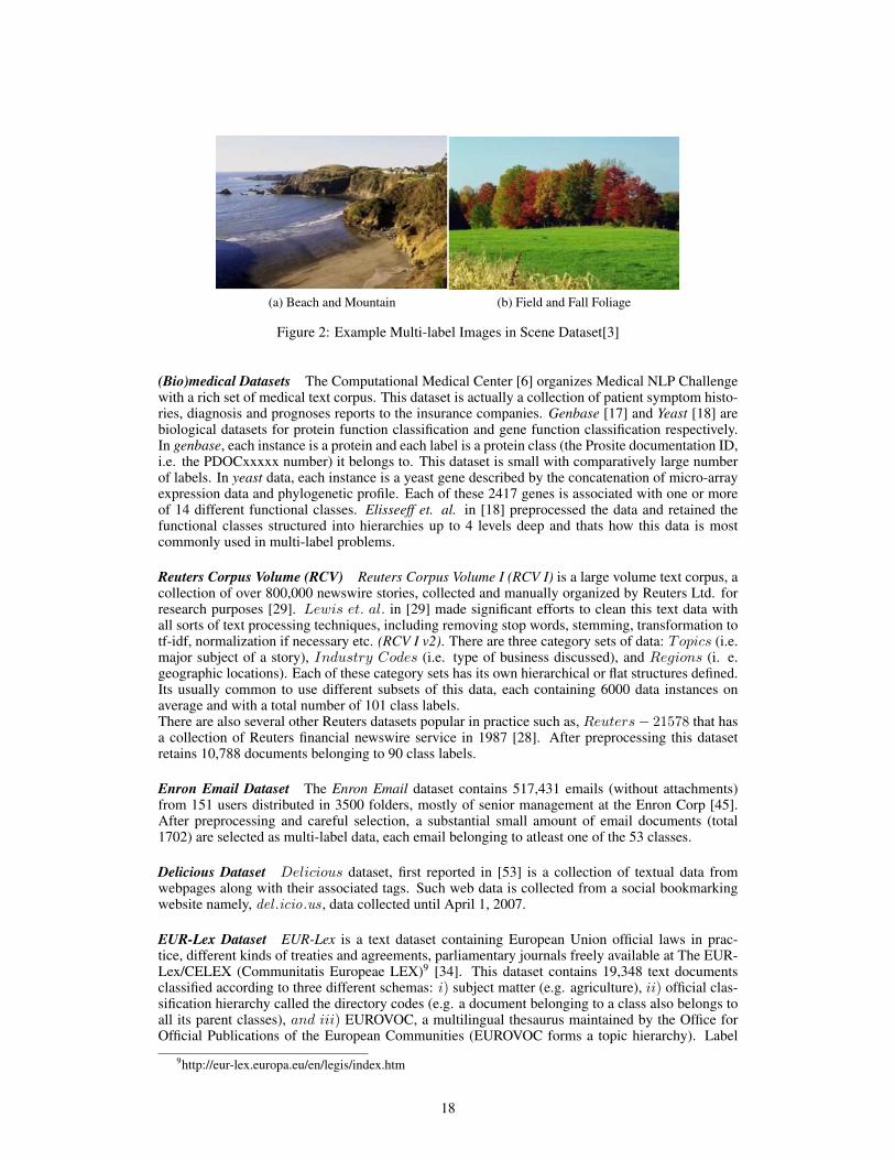
(a) Beach and Mountain (b) Field and Fall Foliage

Figure 2: Example Multi-label Images in Scene Dataset[3]

(Bio)medical Datasets The Computational Medical Center [6] organizes Medical NLP Challengewith a rich set of medical text corpus. This dataset is actually a collection of patient symptom histo-ries, diagnosis and prognoses reports to the insurance companies. Genbase [17] and Yeast [18] arebiological datasets for protein function classification and gene function classification respectively.In genbase, each instance is a protein and each label is a protein class (the Prosite documentation ID,i.e. the PDOCxxxxx number) it belongs to. This dataset is small with comparatively large numberof labels. In yeast data, each instance is a yeast gene described by the concatenation of micro-arrayexpression data and phylogenetic profile. Each of these 2417 genes is associated with one or moreof 14 different functional classes. Elisseeff et. al. in [18] preprocessed the data and retained thefunctional classes structured into hierarchies up to 4 levels deep and thats how this data is mostcommonly used in multi-label problems.

Reuters Corpus Volume (RCV) Reuters Corpus Volume I (RCV I) is a large volume text corpus, acollection of over 800,000 newswire stories, collected and manually organized by Reuters Ltd. forresearch purposes [29]. Lewis et. al. in [29] made significant efforts to clean this text data withall sorts of text processing techniques, including removing stop words, stemming, transformation totf-idf, normalization if necessary etc. (RCV I v2). There are three category sets of data: Topics (i.e.major subject of a story), Industry Codes (i.e. type of business discussed), and Regions (i. e.geographic locations). Each of these category sets has its own hierarchical or flat structures defined.Its usually common to use different subsets of this data, each containing 6000 data instances onaverage and with a total number of 101 class labels.There are also several other Reuters datasets popular in practice such as, Reuters− 21578 that hasa collection of Reuters financial newswire service in 1987 [28]. After preprocessing this datasetretains 10,788 documents belonging to 90 class labels.

Enron Email Dataset The Enron Email dataset contains 517,431 emails (without attachments)from 151 users distributed in 3500 folders, mostly of senior management at the Enron Corp [45].After preprocessing and careful selection, a substantial small amount of email documents (total1702) are selected as multi-label data, each email belonging to atleast one of the 53 classes.

Delicious Dataset Delicious dataset, first reported in [53] is a collection of textual data fromwebpages along with their associated tags. Such web data is collected from a social bookmarkingwebsite namely, del .icio.us , data collected until April 1, 2007.

EUR-Lex Dataset EUR-Lex is a text dataset containing European Union official laws in prac-tice, different kinds of treaties and agreements, parliamentary journals freely available at The EUR-Lex/CELEX (Communitatis Europeae LEX)9 [34]. This dataset contains 19,348 text documentsclassified according to three different schemas: i) subject matter (e.g. agriculture), ii) official clas-sification hierarchy called the directory codes (e.g. a document belonging to a class also belongs toall its parent classes), and iii) EUROVOC, a multilingual thesaurus maintained by the Office forOfficial Publications of the European Communities (EUROVOC forms a topic hierarchy). Label

9http://eur-lex.europa.eu/en/legis/index.htm

18

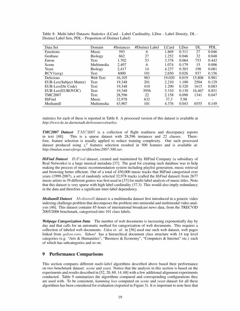
Table 8: Multi-label Datasets Statistics (LCard - Label Cardinality, LDen - Label Density, DL -Distinct Label Sets, PDL - Proportion of Distinct Label)

Data Set Domain #Instances #Distinct Label LCard LDen DL PDLEmotions Music 593 6 1.869 0.311 27 0.046Genbase Biology 662 27 1.252 0.046 32 0.048Enron Text 1,702 53 3.378 0.064 753 0.442Scene Multimedia 2,407 6 1.074 0.179 15 0.006Yeast Biology 2,417 14 4.237 0.303 198 0.081RCV1(avg) Text 6000 101 2.650 0.026 937 0.156Delicious Web Text 16,105 983 19.020 0.019 15,806 0.981EUR-Lex(Subject Matter) Text 19,348 201 2.210 1.100 2504 0.129EUR-Lex(Dir Code) Text 19,348 410 1.290 0.320 1615 0.083EUR-Lex(EUROVOC) Text 19,348 3956 5.310 0.130 16,467 0.851TMC2007 Text 28,596 22 2.158 0.098 1341 0.047HiFind Music 32,978 632 37.3 5.98 - -Mediamill Multimedia 43,907 101 4.376 0.043 6555 0.149

statistics for each of these is reported in Table 8. A processed version of this dataset is available athttp://www.ke.tu-darmstadt.de/resources/eurlex.

TMC2007 Dataset TMC2007 is a collection of flight readiness and discrepancy reportsin text [48]. This is a sparse dataset with 28,596 instances and 22 classes. There-fore, feature selection is usually applied to reduce training complexity. One such processeddataset produced using χ2 features selection resulted in 500 features and is available at:http://mulan.sourceforge.net/files/tmc2007-500.rar.

HiFind Dataset HiFind dataset, created and maintained by HiFind Company (a subsidiary ofReal Networks) is a large musical metadata [37]. The goal for creating such database was to helpmaking the process of music recommendation system including playlist generation, music retrievaland browsing better efficient. Out of a total of 450,000 music tracks that HiFind categorized overyears (1999-2007), a set of randomly selected 32,978 tracks (called the HiFind dataset) from 2677music artists in 39 different genres was first used in [37] for multi-label analysis of music titles. Notethat this dataset is very sparse with high label cardinality (37.3). This would also imply redundancyin the data and therefore a significant inter-label dependency.

Mediamill Dataset Mediamill dataset is a multimedia dataset first introduced in a generic videoindexing challenge problem that decomposes the problem into unimodal and multimodal video anal-ysis [46]. This dataset contains 85 hours of international broadcast news data, from the TRECVID2005/2006 benchmark, categorized into 101 class labels.

Webpage Categorization Data The number of web documents is increasing exponentially day byday and that calls for an automatic method for categorization of web documents. This requires acollection of labeled web documents. Udea et. al. in [56] used one such web dataset, web pageslinked from yahoo.com. Yahoo! has a hierarchical document class structure with 14 top levelcategories (e.g. “Arts & Humanities”, “Business & Economy”, “Computers & Internet” etc.) eachof which has subcategories and so on.

9 Performance Comparisons

This section compares different multi-label algorithms described above based their performanceon two benchmark dataset: scene and yeast. Notice that the analysis in this section is based on theexperiments and results described in [52, 20, 69, 14, 68] with a few additional alignment experimentsconducted. Table 9 summarizes the algorithms compared and corresponding configurations theyare used with. To be consistent, hamming loss computed on scene and yeast dataset for all thesealgorithms has been considered for evaluation (reported in Figure 3). It is important to note here that

19

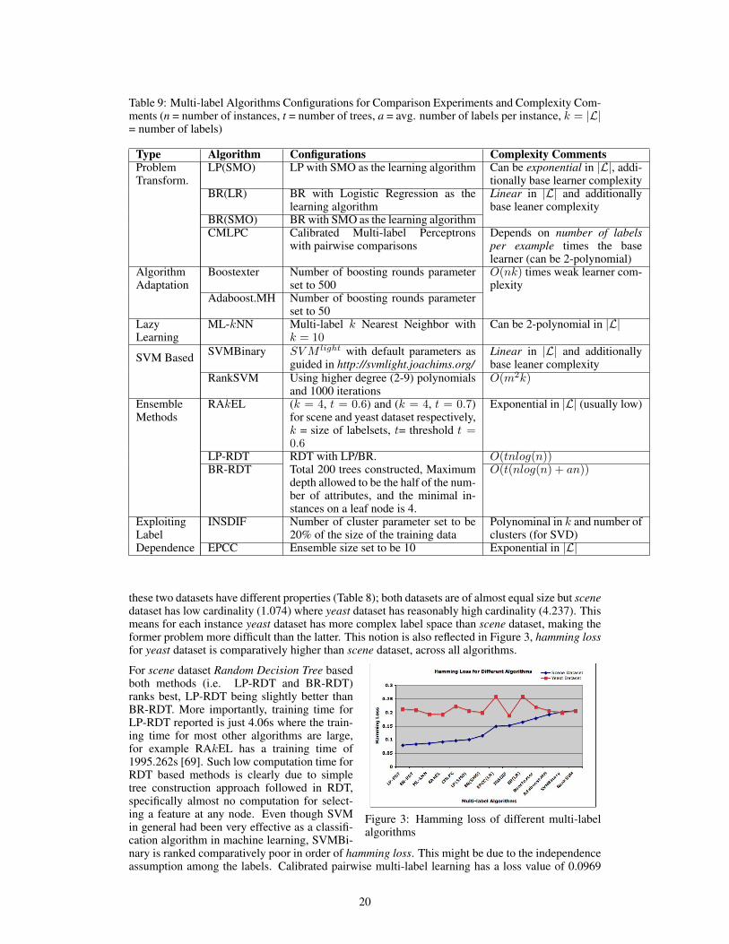
Table 9: Multi-label Algorithms Configurations for Comparison Experiments and Complexity Com-ments (n = number of instances, t = number of trees, a = avg. number of labels per instance, k = |L|= number of labels)

Type Algorithm Configurations Complexity CommentsProblemTransform.

LP(SMO) LP with SMO as the learning algorithm Can be exponential in |L|, addi-tionally base learner complexity

BR(LR) BR with Logistic Regression as thelearning algorithm

Linear in |L| and additionallybase leaner complexity

BR(SMO) BR with SMO as the learning algorithmCMLPC Calibrated Multi-label Perceptrons

with pairwise comparisonsDepends on number of labelsper example times the baselearner (can be 2-polynomial)

AlgorithmAdaptation

Boostexter Number of boosting rounds parameterset to 500

O(nk) times weak learner com-plexity

Adaboost.MH Number of boosting rounds parameterset to 50

LazyLearning

ML-kNN Multi-label k Nearest Neighbor withk = 10

Can be 2-polynomial in |L|

SVM Based SVMBinary SVM light with default parameters asguided in http://svmlight.joachims.org/

Linear in |L| and additionallybase leaner complexity

RankSVM Using higher degree (2-9) polynomialsand 1000 iterations

O(m2k)

EnsembleMethods

RAkEL (k = 4, t = 0.6) and (k = 4, t = 0.7)for scene and yeast dataset respectively,k = size of labelsets, t= threshold t =0.6

Exponential in |L| (usually low)

LP-RDT RDT with LP/BR. O(tnlog(n))BR-RDT Total 200 trees constructed, Maximum

depth allowed to be the half of the num-ber of attributes, and the minimal in-stances on a leaf node is 4.

O(t(nlog(n) + an))

ExploitingLabelDependence

INSDIF Number of cluster parameter set to be20% of the size of the training data

Polynominal in k and number ofclusters (for SVD)

EPCC Ensemble size set to be 10 Exponential in |L|

these two datasets have different properties (Table 8); both datasets are of almost equal size but scenedataset has low cardinality (1.074) where yeast dataset has reasonably high cardinality (4.237). Thismeans for each instance yeast dataset has more complex label space than scene dataset, making theformer problem more difficult than the latter. This notion is also reflected in Figure 3, hamming lossfor yeast dataset is comparatively higher than scene dataset, across all algorithms.

Figure 3: Hamming loss of different multi-labelalgorithms

For scene dataset Random Decision Tree basedboth methods (i.e. LP-RDT and BR-RDT)ranks best, LP-RDT being slightly better thanBR-RDT. More importantly, training time forLP-RDT reported is just 4.06s where the train-ing time for most other algorithms are large,for example RAkEL has a training time of1995.262s [69]. Such low computation time forRDT based methods is clearly due to simpletree construction approach followed in RDT,specifically almost no computation for select-ing a feature at any node. Even though SVMin general had been very effective as a classifi-cation algorithm in machine learning, SVMBi-nary is ranked comparatively poor in order of hamming loss. This might be due to the independenceassumption among the labels. Calibrated pairwise multi-label learning has a loss value of 0.0969

20

which demonstrates the effectiveness of calibration mechanism over ranking by pairwise compar-ison. INSDIF tries of explicitly model the ambiguity in the input space using a bag of instancesrepresentation for each instance and this achieves better performance but is outperformed by en-semble based methods such as RDT and RAkEL. This clearly demonstrates the effectiveness ofensembles on top of modeling label correlations.

In case of slightly more sparse yeast dataset, INSDIF seemed to outperform all others. This alsoillustrates the effectiveness of modeling ambiguity in the input space that is core notion in INSDIF.Performance of ensemble based methods such as RAkEL, are also close to the best. In general,ensemble based methods and that captures the dependencies in the data seemed to perform goodacross both datasets. It is important to note that this comparison presented here is based on hammingloss only, and there are other parameters (described in section 7.1.1) need to be explored for anyspecific application.

Table 9 also reports the computational complexity of each algorithm. Notice that most of the algo-rithms reported are either exponential or polynomial in |L|. Although in most real problems suchcomplexities are expected to be low due to the real data being less sparse (usually less number oflabels, and less number of labels per instance in most applications), they do not really scale verywell with large real world applications and especially not suitable for online problems.

10 Future Works and Conclusions

In this paper, an empirical study of different multi-label algorithms, their applications and evaluationmetrics has been presented. A sparse set of existing algorithms has been organized based on theirworking principle and a comparative performance analysis has been reported. This study providesuseful insights on the relationships among different algorithms and directs light for future research.A few possible future challenges have also been identified: i) while it has been established thatexploiting the label correlations is an important factor for improving the performance, this idea inmost cases has been used intuitively; a future challenge, therefore, is to theoretically explore theconditional and unconditional dependencies and correlate the performance improvement with eachkind of dependence modeling, ii) a number of methods have been quite successful to model smalland medium sparse data with reasonably good performances, however, further research attentionis needed especially to deal with complicated and large data (notice the significant performancedifference reported for yeast and scene dataset), iii) the computational complexities of most of thealgorithms suggest that more efficient algorithms would be needed to achieve scale independence,iv) although it has been established that the data properties such as label cardinality can stronglyaffect the performance of a multi-label algorithm, there is no systematic study on how and why theperformance varies over different data properties; any such study would be helpful to decide onmulti-label algorithms for any particular domain, v) with emerging needs for online algorithms, animportant future direction would be to design efficient online multi-label approaches that scale withlarge and sparse domains.

References

[1] Arindam Banerjee. Scalable clustering algorithms with balancing constraints. Data MiningKnowledge Discovery, 13:2006.

[2] David M. Blei, Andrew Y. Ng, and Michael I. Jordan. Latent dirichlet allocation. J. Mach.Learn. Res., 3:993–1022, March 2003.

[3] M. R. Boutell, J. Luo, X. Shen, and C. M. Brown. Learning multi-label scene classification.Pattern Recognition, 37(9):1757–1771, 2004.

[4] Klaus Brinker and Eyke Hullermeier. Case-Based Multilabel Ranking. In Proceedings of the20th International Conference on Artificial Intelligence (IJCAI ’07), pages 702–707, Hyder-abad, India, 2007.

[5] Rich Caruana. Multitask learning. In Machine Learning, pages 41–75, 1997.

[6] Computational Medical Center. . Medical NLP Challenge,http://www.computationalmedicine.org/challenge/index.php.

21

[7] Nicol Cesa-bianchi, Luca Zaniboni, and Michael Collins. Incremental algorithms for hier-archical classification. In Journal of Machine Learning Research, pages 31–54. MIT Press,2004.

[8] A. Clare and R. D. King. Knowledge Discovery in Multi-Label Phenotype Data. In Proceed-ings of the 5th European Conference on Principles of Data Mining and Knowledge Discovery(PKDD 2001), pages 42–53, Freiburg, Germany, 2001.

[9] Thomas M. Cover and Joy A. Thomas. Elements of information theory. Wiley-Interscience,New York, NY, USA, 1991.

[10] Koby Crammer, Michael Kearns, and Jennifer Wortman. Learning from multiple sources. InIn NIPS, 2007.

[11] Koby Crammer and Yoram Singer. A family of additive online algorithms for category ranking.Journal of Machine Learning Research, 3:1025–1058, 2003.

[12] F. de Comite, R. Gilleron, and M. Tommasi. Learning Multi-label Alternating Decision Treesfrom Texts and Data. In Proceedings of the 3rd International Conference on Machine Learn-ing and Data Mining in Pattern Recognition (MLDM 2003), pages 35–49, Leipzig, Germany,Julym 2003.

[13] Morris H. De Groot. Optimal statistical decisions / Morris H. De Groot. McGraw-Hill, NewYork :,, 1970.

[14] Krzysztof Dembczynski, Weiwei Cheng, and Eyke Hullermeier. Bayes optimal multilabel clas-sification via probabilistic classifier chains. In The 27th International Conference on MachineLearning, pages 279–286, Haifa, Israel, 2010.

[15] Krzysztof Dembczynski, Willem Waegeman, Weiwei Cheng, and Eyke Hullermeier. On labeldependence in multi-label classification. In Workshop Proceedings of Learning from Multi-Label Data, The 27th International Conference on Machine Learning, pages 5–12, Haifa, Is-rael, June 2010.

[16] A. P. Dempster, N. M. Laird, and D. B. Rubin. Maximum likelihood from incomplete data viathe em algorithm. Journal of the Royal Statistical Society, Series B, 39(1):1–38, 1977.

[17] S. Diplaris, G. Tsoumakas, P. Mitkas, and I. Vlahavas. Protein Classification with MultipleAlgorithms. In Proceedings of the 10th Panhellenic Conference on Informatics (PCI 2005),pages 448–456, Volos, Greece, November 2005.

[18] A. Elisseeff and J. Weston. A kernel method for multi-labelled classification. In Advances inNeural Information Processing Systems 14, 2002.

[19] Tom Fawcett. An introduction to roc analysis. Pattern Recogn. Lett., 27:861–874, June 2006.

[20] Johannes Furnkranz, Eyke Hullermeier, Eneldo Lozamencıa, and Klaus Brinker. Multilabelclassification via calibrated label ranking. Machine Learning, 2008.

[21] N. Ghamrawi and A. Mccallum. Collective Multi-Label Classification. In Proceedings ofthe 3005 ACM Conference on Information and Knowledge Management (CIKM ’05), pages195–200, Bremen, Germany, 2005.

[22] S. Godbole and S. Sarawagi. Discriminative Methods for Multi-labeled Classification. InProceedings of the 8th Pacific-Asia Conference on Knowledge Discovery and Data Mining(PAKDD 2004), pages 22–30, 2004.

[23] Xian-Sheng Hua and Guo-Jun Qi. Online multi-label active annotation: towards large-scalecontent-based video search. In Proceeding of the 16th ACM international conference on Mul-timedia, MM ’08, pages 141–150, New York, NY, USA, 2008. ACM.

[24] E. Hullermeier, J. Furnkranz, W. Cheng, and K. Brinker. Label ranking by learning pairwisepreferences. Artificial Intelligence, 172(16-17):1897–1916, November 2008.

[25] Shuiwang Ji, Lei Tang, Shipeng Yu, and Jieping Ye. Extracting shared subspace for multi-label classification. In Proceeding of the 14th ACM SIGKDD international conference onKnowledge discovery and data mining, KDD ’08, pages 381–389, New York, NY, USA, 2008.ACM.

[26] Rong Jin and Zoubin Ghahramani. Learning with multiple labels. In NIPS, pages 897–904,2002.

22

[27] Ron Kohavi and George H. John. Wrappers for feature subset selection. Artif. Intell., 97:273–324, December 1997.

[28] D. D. Lewis. Reuters-21578 text categorization test collection distribution 1.0. 2004.

[29] David D. Lewis, Yiming Yang, Tony G. Rose, and Fan Li. RCV1: A New Benchmark Collec-tion for Text Categorization Research. J. Mach. Learn. Res., 5:361–397, 2004.

[30] Eneldo Loza Mencıa. Multilabel classification in parallel tasks. In Min-Ling Zhang, GrigoriosTsoumakas, and Zhi-Hua Zhou, editors, Working Notes of the 2nd International Workshop onLearning from Multi-Label Data at ICML/COLT 2010, pages 29–36, June 2010.

[31] X. Luo and Zincir A. N. Heywood. Evaluation of Two Systems on Multi-class Multi-label Doc-ument Classification. In Proceedings of the 15th International Symposium on Methodologiesfor Intelligent Systems, pages 161–169, 2005.

[32] A. Mccallum. Multi-label text classification with a mixture model trained by EM. In Proceed-ings of the AAAI’ 99 Workshop on Text Learning, 1999.

[33] Eneldo Loza Menca and Johannes Frnkranz. Pairwise learning of multilabel classificationswith perceptrons. In In: Proceedings of the IEEE World Congress on Computational Intelli-gence (WCCI-08), IEEE (2008.

[34] Eneldo Loza Menca and Johannes Frnkranz. Efficient multilabel classification algorithms forlarge-scale problems in the legal domain. In Proceedings of the Language Resources andEvaluation Conference (LREC) Workshop on Semantic Processing of Legal Texts, 2008.

[35] T. Minka. Expectation propagation for approximate bayesian inference. Ph. D Thesis, MITMedia Labs, 2001.

[36] Ohad Shamir Ofer Dekel. Multiclass-multilabel classification with more classes than examples.In JMLR Workshop and Conference Proceedings Volume 9: AISTATS, pages 137–144, 2010.

[37] F. Pachet and P. Roy. Improving Multilabel Analysis of Music Titles: A Large-Scale Validationof the Correction Approach. Audio, Speech, and Language Processing, IEEE Transactions on,17(2):335–343, 2009.

[38] Cheong Hee Park and Moonhwi Lee. On applying linear discriminant analysis for multi-labeled problems. Pattern Recogn. Lett., 29:878–887, May 2008.

[39] James Petterson and Tiberio Caetano. Reverse multi-label learning. In J. Lafferty, C. K. I.Williams, R. Zemel, J. Shawe-Taylor, and A. Culotta, editors, Advances in Neural InformationProcessing Systems 23, pages 1903–1911. 2010.

[40] Novi Quadrianto, Alexander Smola, Tiberio Caetano, S.V.N. Vishwanathan, and James Pet-terson. Multitask learning without label correspondences. In J. Lafferty, C. K. I. Williams,R. Zemel, J. Shawe-Taylor, and A. Culotta, editors, Advances in Neural Information Process-ing Systems 23, pages 1948–1956. 2010.

[41] J. Read. A Pruned Problem Transformation Method for Multi-label classification. In Proc.2008 New Zealand Computer Science Research Student Conference (NZCSRS 2008), pages143–150, 2008.

[42] Jesse Read, Bernhard Pfahringer, and Geoff Holmes. Multi-label Classification Using En-sembles of Pruned Sets. In ICDM ’08: Proceedings of the 2008 Eighth IEEE InternationalConference on Data Mining, volume 0, pages 995–1000, Washington, DC, USA, 2008. IEEEComputer Society.

[43] Gerard Salton. Developments in automatic text retrieval. Science, 253:974–979, 1991.

[44] Schapire. Boostexter: a boosting-based system for text categorization. Machine Learning,39(2/3):135–168, 2000.

[45] Jitesh Shetty and Jafar Adibi. The enron email dataset database schema and brief statisticalreport, 2004.

[46] Cees G. M. Snoek, Marcel Worring, Jan C. van Gemert, Jan M. Geusebroek, and ArnoldW. M. Smeulders. The challenge problem for automated detection of 101 semantic conceptsin multimedia. In MULTIMEDIA ’06: Proceedings of the 14th annual ACM internationalconference on Multimedia, pages 421–430, New York, NY, USA, 2006. ACM.

23

[47] E. Spyromitros, G. Tsoumakas, and Ioannis Vlahavas. An Empirical Study of Lazy MultilabelClassification Algorithms. In Proc. 5th Hellenic Conference on Artificial Intelligence (SETN2008), pages 401–406. 2008.

[48] Ashok N. Srivastava and Brett Zane-Ulman. Discovering Recurring Anomalies in Text ReportsRegarding Complex Space Systems. In IEEE Aerospace Conference, 2005.

[49] Lei Tang, Suju Rajan, and Vijay K. Narayanan. Large scale multi-label classification viametalabeler. In WWW ’09: Proceedings of the 18th international conference on World wideweb, pages 211–220, New York, NY, USA, 2009. ACM.

[50] F. A. Thabtah, P. Cowling, and Y. Peng. MMAC: A New Multi-class, Multi-label AssociativeClassification Approach. In Proceedings of the 4th IEEE International Conference on DataMining, ICDM ’04, pages 217–224, 2004.

[51] K. Trohidis, G. Tsoumakas, G. Kalliris, and I. Vlahavas. Multilabel Classification of Musicinto Emotions. In Proc. 9th International Conference on Music Information Retrieval (ISMIR2008), Philadelphia, PA, USA, 2008, 2008.

[52] G. Tsoumakas and I. Katakis. Multi-Label Classification: An Overview. International Journalof Data Warehousing and Mining, 3(3):1–13, 2007.

[53] G. Tsoumakas, I. Katakis, and I. Vlahavas. Effective and Efficient Multilabel Classificationin Domains with Large Number of Labels. In Proc. ECML/PKDD 2008 Workshop on MiningMultidimensional Data (MMD’08), 2008.

[54] G. Tsoumakas and I. Vlahavas. Random k-Labelsets: An Ensemble Method for MultilabelClassification. In Proceedings of the 18th European Conference on Machine Learning (ECML2007), pages 406–417, Warsaw, Poland, September 2007.

[55] Grigorios Tsoumakas, Ioannis Katakis, and Ioannis Vlahavas. Mining Multi-label Data. O.Maimon, L. Rokach (Ed.), Springer, 2nd edition, 2010.

[56] N. Ueda and K. Saito. Parametric mixture models for multi-labeled text. In Advances in NeuralInformation Processing Systems 15, Neural Information Processing Systems, NIPS, 2002.

[57] A. Veloso, Jr, M. Goncalves, and M. Zaki. Multi-Label Lazy Associative Classification. InProceedings of the 11th European Conference on Principles and Practice of Knowledge Dis-covery in Databases (PKDD 2007), volume LNAI 4702, pages 605–612, Warsaw, Poland,September 2007. Springer.

[58] Anthony Vetro, Chang Wen Chen, C.C. J. Kuo, Tong Zhang, Qi Tian, and John R. Smith.Content-based audio retrieval: a comparative study of various features and similarity measures.In Proceedings of SPIE, Vol. 6015 Multimedia Systems and Applications VIII, 2005.

[59] Hongning Wang, Minlie Huang, and Xiaoyan Zhu. A generative probabilistic model for multi-label classification. In Proceedings of the 2008 Eighth IEEE International Conference on DataMining, pages 628–637, Washington, DC, USA, 2008. IEEE Computer Society.

[60] Alicja Wieczorkowska, Piotr Synak, and Zbigniew Ras. Multi-Label Classification of Emo-tions in Music. pages 307–315. 2006.

[61] Ralf Herbrich Xinhua Zhang, Thore Graepel. Bayesian online learning for multi-label andmulti-variate performance measures. In International Conference on Artificial Intelligenceand Statistics, (AISTATS), 2010.

[62] Rong Yan, Jelena Tesic, and John R. Smith. Model-shared subspace boosting for multi-labelclassification. In Proceedings of the 13th ACM SIGKDD international conference on Knowl-edge discovery and data mining, KDD ’07, pages 834–843, New York, NY, USA, 2007. ACM.

[63] Yiming Yang. An evaluation of statistical approaches to text categorization. Journal of Infor-mation Retrieval, 1:67–88, 1999.

[64] Kai Yu, Shipeng Yu, and Volker Tresp. Multi-label Informed Latent Semantic Indexing. InSIGIR ’05: Proceedings of the 28th annual international ACM SIGIR conference on Researchand development in information retrieval, pages 258–265, Salvador, Brazil, 2005. ACM Press.

[65] M. L. Zhang and Z. H. Zhou. Multi-Label Neural Networks with Applications to FunctionalGenomics and Text Categorization. IEEE Transactions on Knowledge and Data Engineering,18(10):1338–1351, 2006.

24

[66] Min L. Zhang and Zhi H. Zhou. ML-KNN: A lazy learning approach to multi-label learning.Pattern Recognition, 40(7):2038–2048, July 2007.

[67] Min-Ling Zhang and Kun Zhang. Multi-label learning by exploiting label dependency. InProceedings of the 16th ACM SIGKDD international conference on Knowledge discovery anddata mining, KDD ’10, pages 999–1008, New York, NY, USA, 2010. ACM.

[68] Min-Ling Zhang and Zhi-Hua Zhou. Multi-label learning by instance differentiation. In Pro-ceedings of the 22nd national conference on Artificial intelligence - Volume 1, pages 669–674.AAAI Press, 2007.

[69] Xiatian Zhang, Quan Yuan, Shiwan Zhao, Wei Fan, Wentao Zheng, and Zhong Wang. Multi-label classification without the multi-label cost. In SDM, pages 778–789, 2010.

[70] Zhi H. Zhou and Min L. Zhang. Multi-Instance Multi-Label Learning with Application toScene Classification. In Bernhard Scholkopf, John C. Platt, and Thomas Hoffman, editors,NIPS, pages 1609–1616. MIT Press, 2006.

[71] Shenghuo Zhu, Xiang Ji, Wei Xu, and Yihong Gong. Multi-labelled Classification UsingMaximum Entropy Method. In Proceedings of the 28th annual international ACM SIGIRconference on Research and development in Information Retrieval, pages 274–281, 2005.

25