
A Late Miocene climate model simulation with ECHAM4/ML and its quantitative validation with...
20
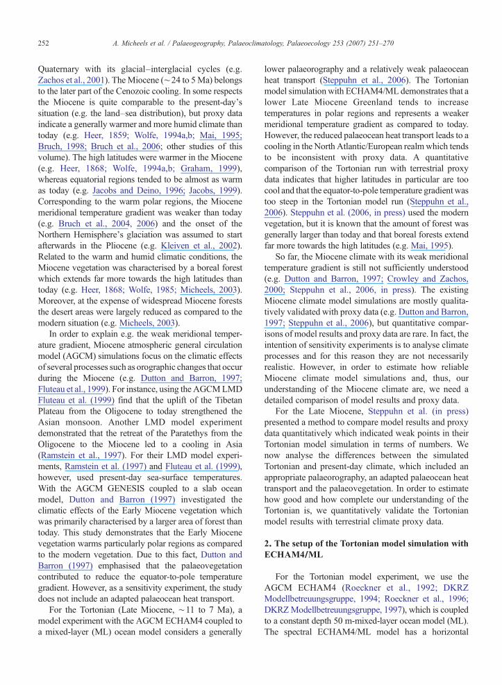
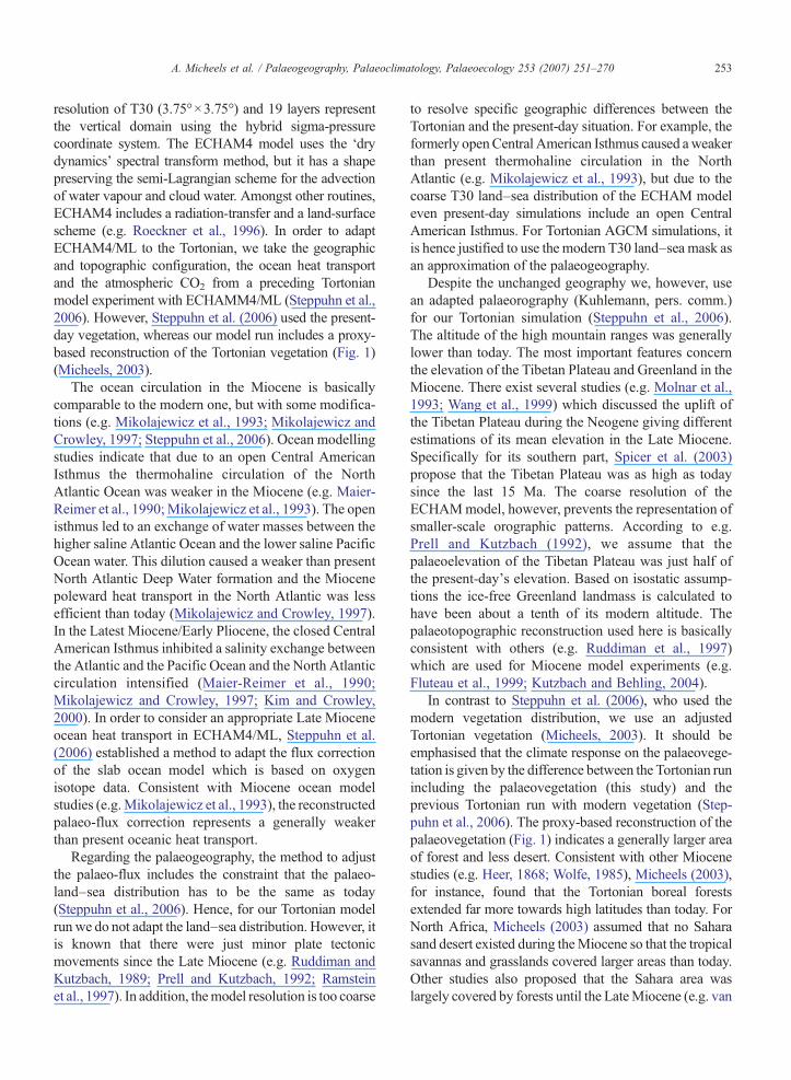
A Late Miocene climate model simulation with ECHAM4/ML and its quantitative validation with terrestrial proxy data Arne Micheels a,b, ⁎ , Angela A. Bruch a,b , Dieter Uhl b,c , Torsten Utescher d , Volker Mosbrugger a a Senckenberg Forschungsinstitut und Naturmuseum, Senckenberganlage 25, D-60325 Frankfurt/Main, Germany b Institut für Geowissenschaften, Universität Tübingen, Sigwartstraße 10, D-72076 Tübingen, Germany c Laboratory of Palaeobotany and Palynology, Utrecht University, Budapestlaan 4, 3584 CD Utrecht, The Netherlands d Geologisches Institut, Universität Bonn, Nußallee 8, D-53115 Bonn, Germany Received 13 December 2004; received in revised form 26 February 2007; accepted 5 March 2007 Abstract For the Tortonian (Late Miocene, 11 to 7 Ma), we present a model simulation using the atmospheric general circulation model (AGCM) ECHAM4 coupled to a mixed-layer (ML) ocean model. The Tortonian simulation with ECHAM4/ML includes an adjusted weaker than present ocean heat transport, a generally lower palaeorography and an appropriate palaeovegetation. We analyse the climatic differences between the Tortonian run and the present-day control experiment, and we validate our Tortonian model results for the mean annual temperature and the annual precipitation with quantitative terrestrial proxy data. Globally, the Tortonian run is slightly warmer (+0.6 °C) and the global precipitation indicates more humid conditions (+ 27 mm/a) than the PD control run. Particularly the northern high latitudes are warmer (+3.5 °C) in the Tortonian simulation which leads to a weaker meridional temperature gradient than today as well as to a reduction of polar sea ice. We attribute the polar warming to the lowering of the Greenland elevation (+ 20 °C) in the Miocene and to the effects of the palaeovegetation. The reduced altitude of the Tibetan Plateau causes a warming (+20 °C) as compared to today and leads to a weaker Asian monsoon in the Tortonian run. For Europe, the mean annual temperature is almost unaffected as compared to today because a cooling effect of the weak palaeocean heat transport is compensated by the palaeovegetation. When validating our model results, we find that the Tortonian run is largely consistent with quantitative proxy data. However, the high latitudes tend to be generally too cool in the palaeoclimate simulation and the equator-to- pole temperature gradient is too steep as compared to proxy data. For Europe the comparison with proxy data indicates that the Tortonian simulation underestimates the mean annual temperatures, but precipitation patterns are quite consistent between model results and proxy data. Overall, the Tortonian run is quite realistic and hence the model simulation contributes to a better understanding of the relevant climate processes in the Miocene. However, the discrepancies to proxy data demonstrate that we still do not sufficiently understand the Late Miocene climate. © 2007 Elsevier B.V. All rights reserved. Keywords: Late Miocene; Climate modelling; Quantitative model validation; Terrestrial proxy data 1. Introduction The Cenozoic climate is characterised by the transi- tion from the warm and humid Cretaceous to the cool Palaeogeography, Palaeoclimatology, Palaeoecology 253 (2007) 251 – 270 www.elsevier.com/locate/palaeo ⁎ Corresponding author. Senckenberg Forschungsinstitut und Nat- urmuseum, Senckenberganlage 25, D-60325 Frankfurt/Main, Germany. E-mail address: [email protected] (A. Micheels). 0031-0182/$ - see front matter © 2007 Elsevier B.V. All rights reserved. doi:10.1016/j.palaeo.2007.03.042
-
Upload
uni-tuebingen -
Category
Documents
-
view
3 -
download
0
Transcript of A Late Miocene climate model simulation with ECHAM4/ML and its quantitative validation with...

laeoecology 253 (2007) 251–270www.elsevier.com/locate/palaeo
Palaeogeography, Palaeoclimatology, Pa
A Late Miocene climate model simulation with ECHAM4/MLand its quantitative validation with terrestrial proxy data
Arne Micheels a,b,⁎, Angela A. Bruch a,b, Dieter Uhl b,c,Torsten Utescher d, Volker Mosbrugger a
a Senckenberg Forschungsinstitut und Naturmuseum, Senckenberganlage 25, D-60325 Frankfurt/Main, Germanyb Institut für Geowissenschaften, Universität Tübingen, Sigwartstraße 10, D-72076 Tübingen, Germany
c Laboratory of Palaeobotany and Palynology, Utrecht University, Budapestlaan 4, 3584 CD Utrecht, The Netherlandsd Geologisches Institut, Universität Bonn, Nußallee 8, D-53115 Bonn, Germany
Received 13 December 2004; received in revised form 26 February 2007; accepted 5 March 2007
Abstract
For the Tortonian (Late Miocene, 11 to 7 Ma), we present a model simulation using the atmospheric general circulation model(AGCM) ECHAM4 coupled to a mixed-layer (ML) ocean model. The Tortonian simulation with ECHAM4/ML includes an adjustedweaker than present ocean heat transport, a generally lower palaeorography and an appropriate palaeovegetation. We analyse theclimatic differences between the Tortonian run and the present-day control experiment, and we validate our Tortonian model resultsfor the mean annual temperature and the annual precipitation with quantitative terrestrial proxy data. Globally, the Tortonian run isslightly warmer (+0.6 °C) and the global precipitation indicates more humid conditions (+27 mm/a) than the PD control run.Particularly the northern high latitudes are warmer (+3.5 °C) in the Tortonian simulation which leads to a weaker meridionaltemperature gradient than today as well as to a reduction of polar sea ice. We attribute the polar warming to the lowering of theGreenland elevation (+20 °C) in the Miocene and to the effects of the palaeovegetation. The reduced altitude of the Tibetan Plateaucauses a warming (+20 °C) as compared to today and leads to a weaker Asian monsoon in the Tortonian run. For Europe, the meanannual temperature is almost unaffected as compared to today because a cooling effect of the weak palaeocean heat transport iscompensated by the palaeovegetation. When validating our model results, we find that the Tortonian run is largely consistent withquantitative proxy data. However, the high latitudes tend to be generally too cool in the palaeoclimate simulation and the equator-to-pole temperature gradient is too steep as compared to proxy data. For Europe the comparison with proxy data indicates that theTortonian simulation underestimates the mean annual temperatures, but precipitation patterns are quite consistent between modelresults and proxy data. Overall, the Tortonian run is quite realistic and hence the model simulation contributes to a betterunderstanding of the relevant climate processes in theMiocene. However, the discrepancies to proxy data demonstrate that we still donot sufficiently understand the Late Miocene climate.© 2007 Elsevier B.V. All rights reserved.
Keywords: Late Miocene; Climate modelling; Quantitative model validation; Terrestrial proxy data
⁎ Corresponding author. Senckenberg Forschungsinstitut und Nat-urmuseum, Senckenberganlage 25, D-60325 Frankfurt/Main,Germany.
E-mail address: [email protected] (A. Micheels).
0031-0182/$ - see front matter © 2007 Elsevier B.V. All rights reserved.doi:10.1016/j.palaeo.2007.03.042
1. Introduction
The Cenozoic climate is characterised by the transi-tion from the warm and humid Cretaceous to the cool
252 A. Micheels et al. / Palaeogeography, Palaeoclimatology, Palaeoecology 253 (2007) 251–270
Quaternary with its glacial–interglacial cycles (e.g.Zachos et al., 2001). TheMiocene (∼24 to 5Ma) belongsto the later part of the Cenozoic cooling. In some respectsthe Miocene is quite comparable to the present-day'ssituation (e.g. the land–sea distribution), but proxy dataindicate a generally warmer and more humid climate thantoday (e.g. Heer, 1859; Wolfe, 1994a,b; Mai, 1995;Bruch, 1998; Bruch et al., 2006; other studies of thisvolume). The high latitudes were warmer in the Miocene(e.g. Heer, 1868; Wolfe, 1994a,b; Graham, 1999),whereas equatorial regions tended to be almost as warmas today (e.g. Jacobs and Deino, 1996; Jacobs, 1999).Corresponding to the warm polar regions, the Miocenemeridional temperature gradient was weaker than today(e.g. Bruch et al., 2004, 2006) and the onset of theNorthern Hemisphere's glaciation was assumed to startafterwards in the Pliocene (e.g. Kleiven et al., 2002).Related to the warm and humid climatic conditions, theMiocene vegetation was characterised by a boreal forestwhich extends far more towards the high latitudes thantoday (e.g. Heer, 1868; Wolfe, 1985; Micheels, 2003).Moreover, at the expense of widespread Miocene foreststhe desert areas were largely reduced as compared to themodern situation (e.g. Micheels, 2003).
In order to explain e.g. the weak meridional temper-ature gradient, Miocene atmospheric general circulationmodel (AGCM) simulations focus on the climatic effectsof several processes such as orographic changes that occurduring the Miocene (e.g. Dutton and Barron, 1997;Fluteau et al., 1999). For instance, using the AGCMLMDFluteau et al. (1999) find that the uplift of the TibetanPlateau from the Oligocene to today strengthened theAsian monsoon. Another LMD model experimentdemonstrated that the retreat of the Paratethys from theOligocene to the Miocene led to a cooling in Asia(Ramstein et al., 1997). For their LMD model experi-ments, Ramstein et al. (1997) and Fluteau et al. (1999),however, used present-day sea-surface temperatures.With the AGCM GENESIS coupled to a slab oceanmodel, Dutton and Barron (1997) investigated theclimatic effects of the Early Miocene vegetation whichwas primarily characterised by a larger area of forest thantoday. This study demonstrates that the Early Miocenevegetation warms particularly polar regions as comparedto the modern vegetation. Due to this fact, Dutton andBarron (1997) emphasised that the palaeovegetationcontributed to reduce the equator-to-pole temperaturegradient. However, as a sensitivity experiment, the studydoes not include an adapted palaeocean heat transport.
For the Tortonian (Late Miocene, ∼11 to 7 Ma), amodel experiment with the AGCM ECHAM4 coupled toa mixed-layer (ML) ocean model considers a generally
lower palaeorography and a relatively weak palaeoceanheat transport (Steppuhn et al., 2006). The Tortonianmodel simulationwith ECHAM4/ML demonstrates that alower Late Miocene Greenland tends to increasetemperatures in polar regions and represents a weakermeridional temperature gradient as compared to today.However, the reduced palaeocean heat transport leads to acooling in the North Atlantic/European realmwhich tendsto be inconsistent with proxy data. A quantitativecomparison of the Tortonian run with terrestrial proxydata indicates that higher latitudes in particular are toocool and that the equator-to-pole temperature gradientwastoo steep in the Tortonian model run (Steppuhn et al.,2006). Steppuhn et al. (2006, in press) used the modernvegetation, but it is known that the amount of forest wasgenerally larger than today and that boreal forests extendfar more towards the high latitudes (e.g. Mai, 1995).
So far, the Miocene climate with its weak meridionaltemperature gradient is still not sufficiently understood(e.g. Dutton and Barron, 1997; Crowley and Zachos,2000; Steppuhn et al., 2006, in press). The existingMiocene climate model simulations are mostly qualita-tively validated with proxy data (e.g. Dutton and Barron,1997; Steppuhn et al., 2006), but quantitative compar-isons of model results and proxy data are rare. In fact, theintention of sensitivity experiments is to analyse climateprocesses and for this reason they are not necessarilyrealistic. However, in order to estimate how reliableMiocene climate model simulations and, thus, ourunderstanding of the Miocene climate are, we need adetailed comparison of model results and proxy data.
For the Late Miocene, Steppuhn et al. (in press)presented a method to compare model results and proxydata quantitatively which indicated weak points in theirTortonian model simulation in terms of numbers. Wenow analyse the differences between the simulatedTortonian and present-day climate, which included anappropriate palaeorography, an adapted palaeocean heattransport and the palaeovegetation. In order to estimatehow good and how complete our understanding of theTortonian is, we quantitatively validate the Tortonianmodel results with terrestrial climate proxy data.
2. The setup of the Tortonian model simulation withECHAM4/ML
For the Tortonian model experiment, we use theAGCM ECHAM4 (Roeckner et al., 1992; DKRZModellbetreuungsgruppe, 1994; Roeckner et al., 1996;DKRZModellbetreuungsgruppe, 1997), which is coupledto a constant depth 50 m-mixed-layer ocean model (ML).The spectral ECHAM4/ML model has a horizontal
253A. Micheels et al. / Palaeogeography, Palaeoclimatology, Palaeoecology 253 (2007) 251–270
resolution of T30 (3.75°×3.75°) and 19 layers representthe vertical domain using the hybrid sigma-pressurecoordinate system. The ECHAM4 model uses the ‘drydynamics’ spectral transform method, but it has a shapepreserving the semi-Lagrangian scheme for the advectionof water vapour and cloud water. Amongst other routines,ECHAM4 includes a radiation-transfer and a land-surfacescheme (e.g. Roeckner et al., 1996). In order to adaptECHAM4/ML to the Tortonian, we take the geographicand topographic configuration, the ocean heat transportand the atmospheric CO2 from a preceding Tortonianmodel experiment with ECHAMM4/ML (Steppuhn et al.,2006). However, Steppuhn et al. (2006) used the present-day vegetation, whereas our model run includes a proxy-based reconstruction of the Tortonian vegetation (Fig. 1)(Micheels, 2003).
The ocean circulation in the Miocene is basicallycomparable to the modern one, but with some modifica-tions (e.g. Mikolajewicz et al., 1993; Mikolajewicz andCrowley, 1997; Steppuhn et al., 2006). Ocean modellingstudies indicate that due to an open Central AmericanIsthmus the thermohaline circulation of the NorthAtlantic Ocean was weaker in the Miocene (e.g. Maier-Reimer et al., 1990;Mikolajewicz et al., 1993). The openisthmus led to an exchange of water masses between thehigher saline Atlantic Ocean and the lower saline PacificOcean water. This dilution caused a weaker than presentNorth Atlantic Deep Water formation and the Miocenepoleward heat transport in the North Atlantic was lessefficient than today (Mikolajewicz and Crowley, 1997).In the Latest Miocene/Early Pliocene, the closed CentralAmerican Isthmus inhibited a salinity exchange betweenthe Atlantic and the Pacific Ocean and the North Atlanticcirculation intensified (Maier-Reimer et al., 1990;Mikolajewicz and Crowley, 1997; Kim and Crowley,2000). In order to consider an appropriate Late Mioceneocean heat transport in ECHAM4/ML, Steppuhn et al.(2006) established a method to adapt the flux correctionof the slab ocean model which is based on oxygenisotope data. Consistent with Miocene ocean modelstudies (e.g.Mikolajewicz et al., 1993), the reconstructedpalaeo-flux correction represents a generally weakerthan present oceanic heat transport.
Regarding the palaeogeography, the method to adjustthe palaeo-flux includes the constraint that the palaeo-land–sea distribution has to be the same as today(Steppuhn et al., 2006). Hence, for our Tortonian modelrun we do not adapt the land–sea distribution. However, itis known that there were just minor plate tectonicmovements since the Late Miocene (e.g. Ruddiman andKutzbach, 1989; Prell and Kutzbach, 1992; Ramsteinet al., 1997). In addition, themodel resolution is too coarse
to resolve specific geographic differences between theTortonian and the present-day situation. For example, theformerly openCentral American Isthmus caused a weakerthan present thermohaline circulation in the NorthAtlantic (e.g. Mikolajewicz et al., 1993), but due to thecoarse T30 land–sea distribution of the ECHAM modeleven present-day simulations include an open CentralAmerican Isthmus. For Tortonian AGCM simulations, itis hence justified to use the modern T30 land–sea mask asan approximation of the palaeogeography.
Despite the unchanged geography we, however, usean adapted palaeorography (Kuhlemann, pers. comm.)for our Tortonian simulation (Steppuhn et al., 2006).The altitude of the high mountain ranges was generallylower than today. The most important features concernthe elevation of the Tibetan Plateau and Greenland in theMiocene. There exist several studies (e.g. Molnar et al.,1993; Wang et al., 1999) which discussed the uplift ofthe Tibetan Plateau during the Neogene giving differentestimations of its mean elevation in the Late Miocene.Specifically for its southern part, Spicer et al. (2003)propose that the Tibetan Plateau was as high as todaysince the last 15 Ma. The coarse resolution of theECHAMmodel, however, prevents the representation ofsmaller-scale orographic patterns. According to e.g.Prell and Kutzbach (1992), we assume that thepalaeoelevation of the Tibetan Plateau was just half ofthe present-day's elevation. Based on isostatic assump-tions the ice-free Greenland landmass is calculated tohave been about a tenth of its modern altitude. Thepalaeotopographic reconstruction used here is basicallyconsistent with others (e.g. Ruddiman et al., 1997)which are used for Miocene model experiments (e.g.Fluteau et al., 1999; Kutzbach and Behling, 2004).
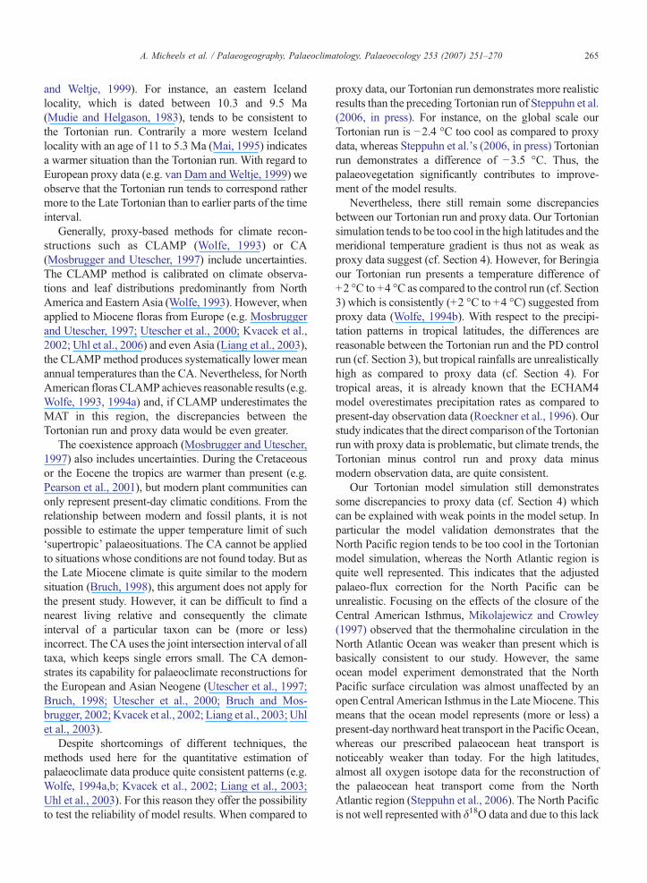
In contrast to Steppuhn et al. (2006), who used themodern vegetation distribution, we use an adjustedTortonian vegetation (Micheels, 2003). It should beemphasised that the climate response on the palaeovege-tation is given by the difference between the Tortonian runincluding the palaeovegetation (this study) and theprevious Tortonian run with modern vegetation (Step-puhn et al., 2006). The proxy-based reconstruction of thepalaeovegetation (Fig. 1) indicates a generally larger areaof forest and less desert. Consistent with other Miocenestudies (e.g. Heer, 1868; Wolfe, 1985), Micheels (2003),for instance, found that the Tortonian boreal forestsextended far more towards high latitudes than today. ForNorth Africa, Micheels (2003) assumed that no Saharasand desert existed during theMiocene so that the tropicalsavannas and grasslands covered larger areas than today.Other studies also proposed that the Sahara area waslargely covered by forests until the LateMiocene (e.g. van
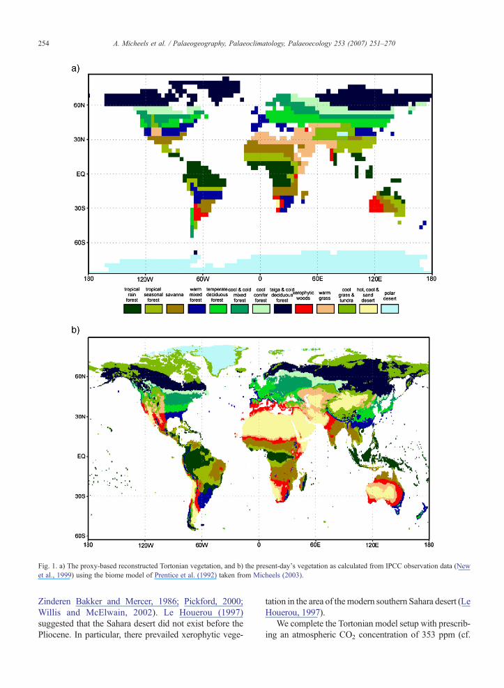
Fig. 1. a) The proxy-based reconstructed Tortonian vegetation, and b) the present-day's vegetation as calculated from IPCC observation data (Newet al., 1999) using the biome model of Prentice et al. (1992) taken from Micheels (2003).
254 A. Micheels et al. / Palaeogeography, Palaeoclimatology, Palaeoecology 253 (2007) 251–270
Zinderen Bakker and Mercer, 1986; Pickford, 2000;Willis and McElwain, 2002). Le Houerou (1997)suggested that the Sahara desert did not exist before thePliocene. In particular, there prevailed xerophytic vege-
tation in the area of themodern southern Sahara desert (LeHouerou, 1997).
We complete the Tortonian model setup with prescrib-ing an atmospheric CO2 concentration of 353 ppm (cf.
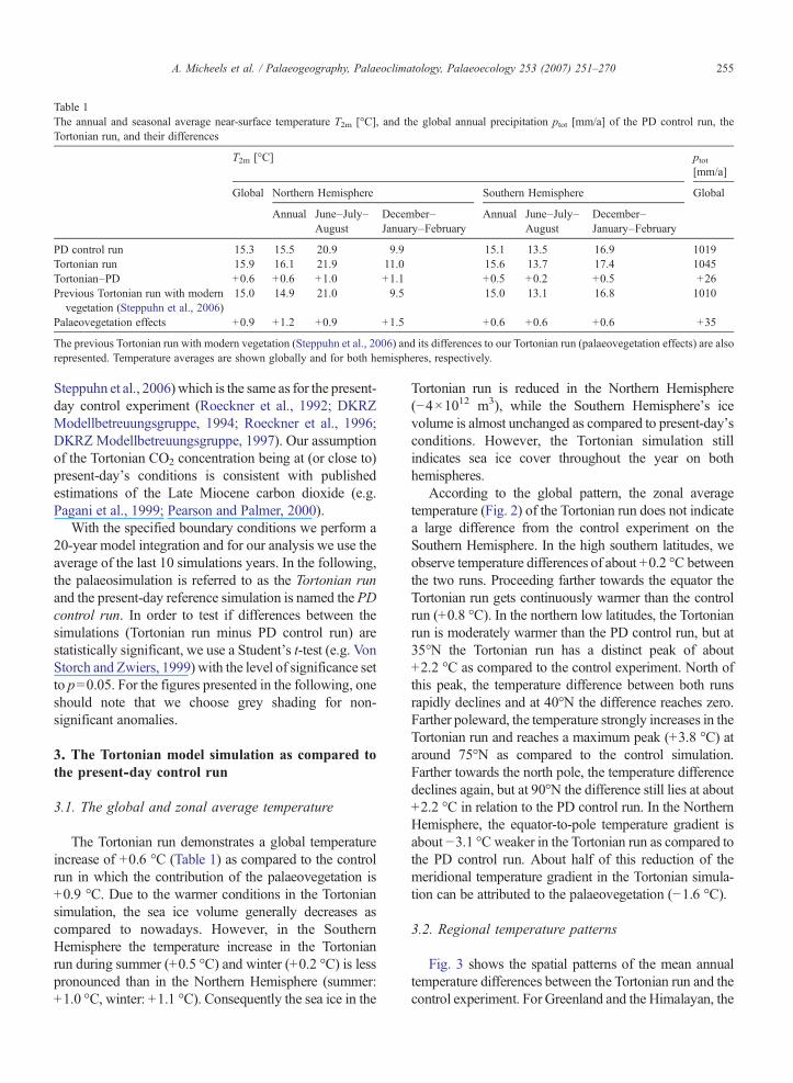
Table 1The annual and seasonal average near-surface temperature T2m [°C], and the global annual precipitation ptot [mm/a] of the PD control run, theTortonian run, and their differences
T2m [°C] ptot[mm/a]
Global Northern Hemisphere Southern Hemisphere Global
Annual June–July–August
December–January–February
Annual June–July–August
December–January–February
PD control run 15.3 15.5 20.9 9.9 15.1 13.5 16.9 1019Tortonian run 15.9 16.1 21.9 11.0 15.6 13.7 17.4 1045Tortonian–PD +0.6 +0.6 +1.0 +1.1 +0.5 +0.2 +0.5 +26Previous Tortonian run with modern
vegetation (Steppuhn et al., 2006)15.0 14.9 21.0 9.5 15.0 13.1 16.8 1010
Palaeovegetation effects +0.9 +1.2 +0.9 +1.5 +0.6 +0.6 +0.6 +35
The previous Tortonian run with modern vegetation (Steppuhn et al., 2006) and its differences to our Tortonian run (palaeovegetation effects) are alsorepresented. Temperature averages are shown globally and for both hemispheres, respectively.
255A. Micheels et al. / Palaeogeography, Palaeoclimatology, Palaeoecology 253 (2007) 251–270
Steppuhn et al., 2006)which is the same as for the present-day control experiment (Roeckner et al., 1992; DKRZModellbetreuungsgruppe, 1994; Roeckner et al., 1996;DKRZ Modellbetreuungsgruppe, 1997). Our assumptionof the Tortonian CO2 concentration being at (or close to)present-day's conditions is consistent with publishedestimations of the Late Miocene carbon dioxide (e.g.Pagani et al., 1999; Pearson and Palmer, 2000).
With the specified boundary conditions we perform a20-year model integration and for our analysis we use theaverage of the last 10 simulations years. In the following,the palaeosimulation is referred to as the Tortonian runand the present-day reference simulation is named the PDcontrol run. In order to test if differences between thesimulations (Tortonian run minus PD control run) arestatistically significant, we use a Student's t-test (e.g. VonStorch and Zwiers, 1999) with the level of significance setto p=0.05. For the figures presented in the following, oneshould note that we choose grey shading for non-significant anomalies.
3. The Tortonian model simulation as compared tothe present-day control run
3.1. The global and zonal average temperature
The Tortonian run demonstrates a global temperatureincrease of +0.6 °C (Table 1) as compared to the controlrun in which the contribution of the palaeovegetation is+0.9 °C. Due to the warmer conditions in the Tortoniansimulation, the sea ice volume generally decreases ascompared to nowadays. However, in the SouthernHemisphere the temperature increase in the Tortonianrun during summer (+0.5 °C) and winter (+0.2 °C) is lesspronounced than in the Northern Hemisphere (summer:+1.0 °C, winter: +1.1 °C). Consequently the sea ice in the
Tortonian run is reduced in the Northern Hemisphere(−4×10¹² m3), while the Southern Hemisphere's icevolume is almost unchanged as compared to present-day'sconditions. However, the Tortonian simulation stillindicates sea ice cover throughout the year on bothhemispheres.
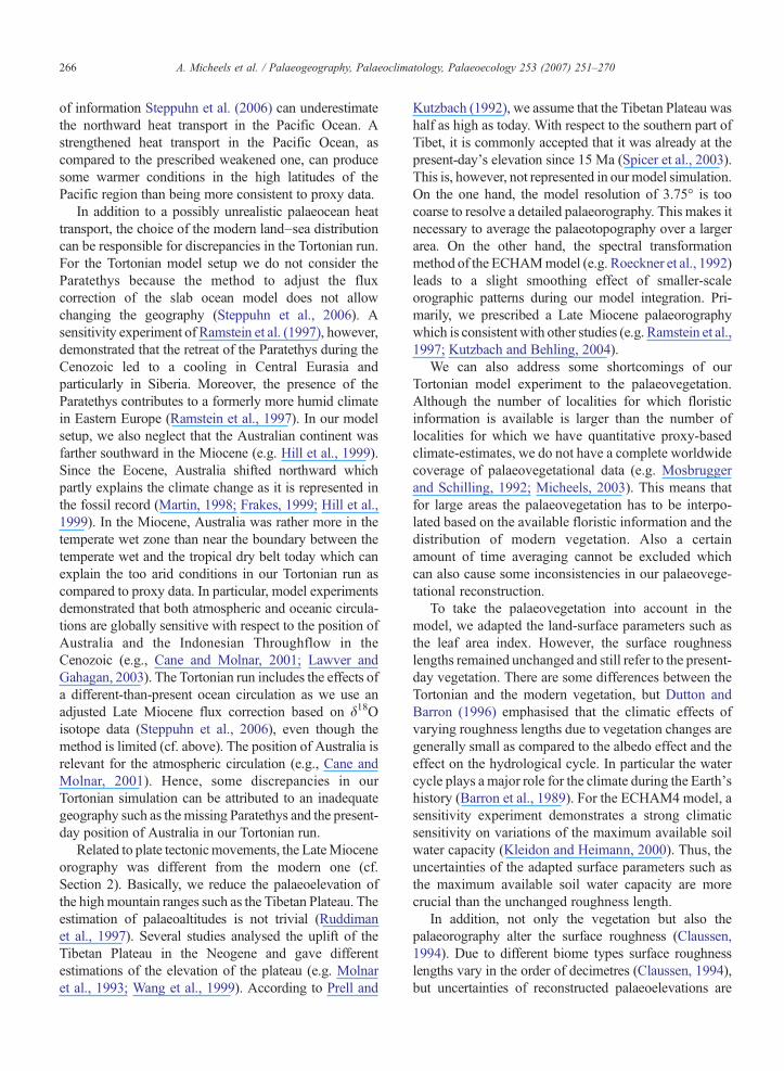
According to the global pattern, the zonal averagetemperature (Fig. 2) of the Tortonian run does not indicatea large difference from the control experiment on theSouthern Hemisphere. In the high southern latitudes, weobserve temperature differences of about +0.2 °C betweenthe two runs. Proceeding farther towards the equator theTortonian run gets continuously warmer than the controlrun (+0.8 °C). In the northern low latitudes, the Tortonianrun is moderately warmer than the PD control run, but at35°N the Tortonian run has a distinct peak of about+2.2 °C as compared to the control experiment. North ofthis peak, the temperature difference between both runsrapidly declines and at 40°N the difference reaches zero.Farther poleward, the temperature strongly increases in theTortonian run and reaches a maximum peak (+3.8 °C) ataround 75°N as compared to the control simulation.Farther towards the north pole, the temperature differencedeclines again, but at 90°N the difference still lies at about+2.2 °C in relation to the PD control run. In the NorthernHemisphere, the equator-to-pole temperature gradient isabout −3.1 °C weaker in the Tortonian run as compared tothe PD control run. About half of this reduction of themeridional temperature gradient in the Tortonian simula-tion can be attributed to the palaeovegetation (−1.6 °C).
3.2. Regional temperature patterns
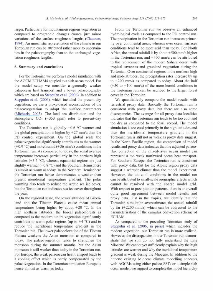
Fig. 3 shows the spatial patterns of the mean annualtemperature differences between the Tortonian run and thecontrol experiment. For Greenland and the Himalayan, the
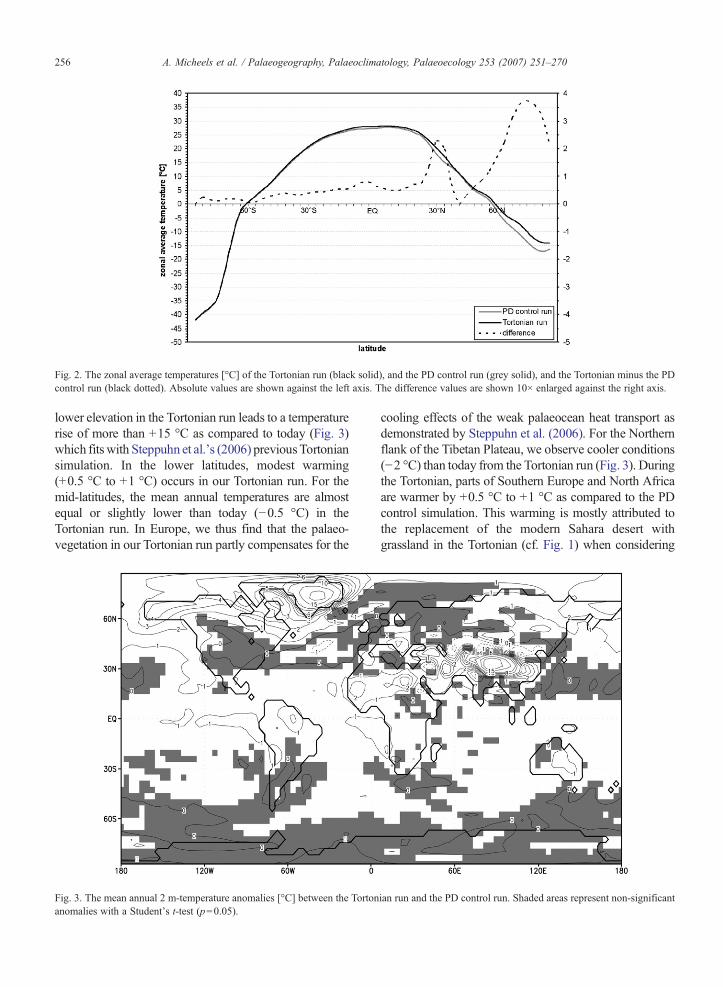
Fig. 2. The zonal average temperatures [°C] of the Tortonian run (black solid), and the PD control run (grey solid), and the Tortonian minus the PDcontrol run (black dotted). Absolute values are shown against the left axis. The difference values are shown 10× enlarged against the right axis.
256 A. Micheels et al. / Palaeogeography, Palaeoclimatology, Palaeoecology 253 (2007) 251–270
lower elevation in the Tortonian run leads to a temperaturerise of more than +15 °C as compared to today (Fig. 3)which fits with Steppuhn et al.'s (2006) previousTortoniansimulation. In the lower latitudes, modest warming(+0.5 °C to +1 °C) occurs in our Tortonian run. For themid-latitudes, the mean annual temperatures are almostequal or slightly lower than today (−0.5 °C) in theTortonian run. In Europe, we thus find that the palaeo-vegetation in our Tortonian run partly compensates for the
Fig. 3. The mean annual 2 m-temperature anomalies [°C] between the Tortonanomalies with a Student's t-test (p=0.05).
cooling effects of the weak palaeocean heat transport asdemonstrated by Steppuhn et al. (2006). For the Northernflank of the Tibetan Plateau, we observe cooler conditions(−2 °C) than today from the Tortonian run (Fig. 3). Duringthe Tortonian, parts of Southern Europe and North Africaare warmer by +0.5 °C to +1 °C as compared to the PDcontrol simulation. This warming is mostly attributed tothe replacement of the modern Sahara desert withgrassland in the Tortonian (cf. Fig. 1) when considering
ian run and the PD control run. Shaded areas represent non-significant
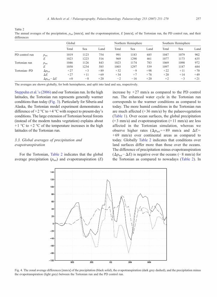
Table 2The annual averages of the precipitation, ptot [mm/a], and the evapotranspiration, E [mm/a], of the Tortonian run, the PD control run, and theirdifferences
Global Northern Hemisphere Southern Hemisphere
Total Sea Land Total Sea Land Total Sea Land
PD control run ptot 1019 1123 754 991 1183 685 1047 1079 902E 1023 1223 516 969 1290 461 1077 1173 635
Tortonian run ptot 1046 1126 843 1023 1174 783 1069 1090 972E 1050 1234 585 1003 1297 539 1097 1187 684
Tortonian–PD Δptot +27 +3 +89 +32 −9 +98 +22 +11 +70ΔE +27 +11 +69 +34 +7 +78 +20 +14 +49Δptot−ΔE ±0 −8 +20 −2 −16 +20 +2 −3 +21
The averages are shown globally, for both hemispheres, and split into land and sea, respectively.
257A. Micheels et al. / Palaeogeography, Palaeoclimatology, Palaeoecology 253 (2007) 251–270
Steppuhn et al.'s (2006) and our Tortonian run. In the highlatitudes, the Tortonian run represents generally warmerconditions than today (Fig. 3). Particularly for Siberia andAlaska, the Tortonian model experiment demonstrates adifference of +2 °C to +4 °C with respect to present-day'sconditions. The large extension of Tortonian boreal forests(instead of the modern tundra vegetation) explains about+1 °C to +2 °C of the temperature increases in the highlatitudes of the Tortonian run.
3.3. Global averages of precipitation andevapotranspiration
For the Tortonian, Table 2 indicates that the globalaverage precipitation (ptot) and evapotranspiration (E)
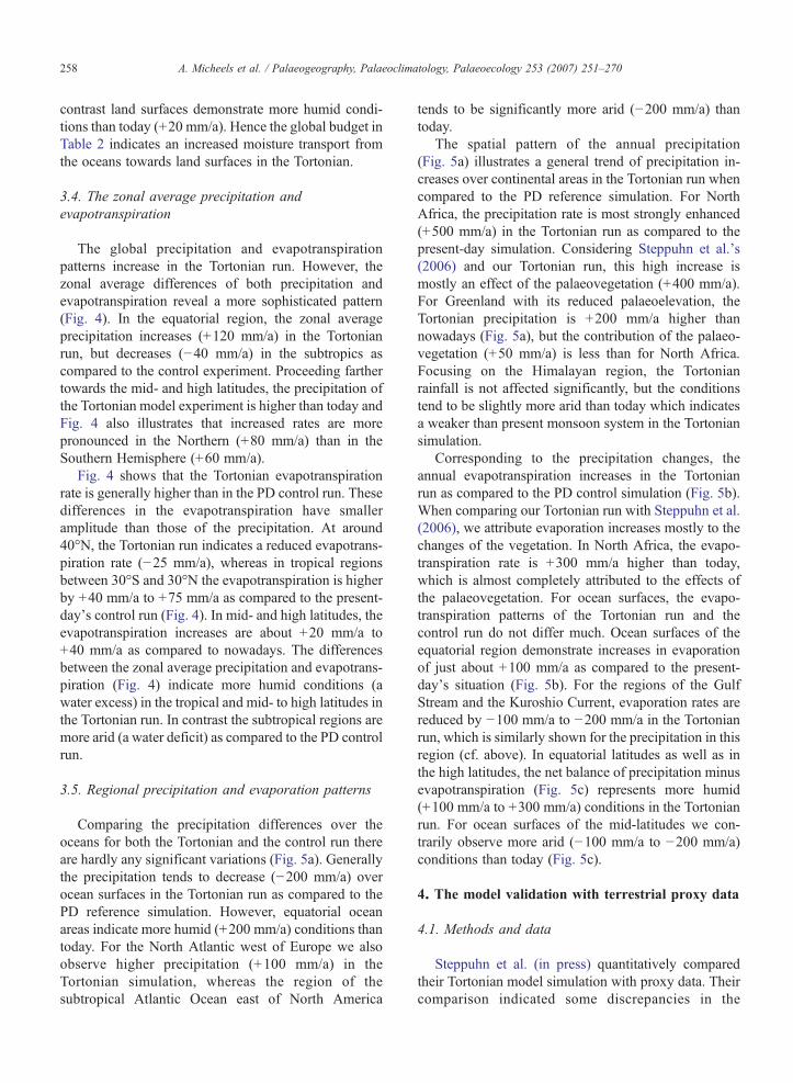
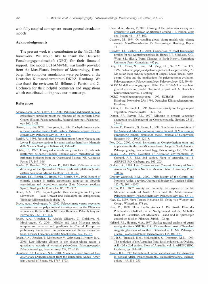
Fig. 4. The zonal average differences [mm/a] of the precipitation (black solid)the evapotranspiration (light grey) between the Tortonian run and the PD co
increase by +27 mm/a as compared to the PD controlrun. The enhanced water cycle in the Tortonian runcorresponds to the warmer conditions as compared totoday. The more humid conditions in the Tortonian runare much affected (+36 mm/a) by the palaeovegetation(Table 1). Over ocean surfaces, the global precipitation(+3 mm/a) and evapotranspiration (+11 mm/a) are lessaffected in the Tortonian simulation, whereas weobserve higher rates (Δptot =+89 mm/a and ΔE=+69 mm/a) over continental areas as compared totoday. Globally Table 2 indicates that conditions overland surfaces differ more than those over the oceans.The difference of precipitation minus evapotranspiration(Δptot−ΔE) is negative over the oceans (−8 mm/a) forthe Tortonian as compared to nowadays (Table 2). In
, the evapotranspiration (dark grey dashed), and the precipitation minusntrol run.
258 A. Micheels et al. / Palaeogeography, Palaeoclimatology, Palaeoecology 253 (2007) 251–270
contrast land surfaces demonstrate more humid condi-tions than today (+20 mm/a). Hence the global budget inTable 2 indicates an increased moisture transport fromthe oceans towards land surfaces in the Tortonian.
3.4. The zonal average precipitation andevapotranspiration
The global precipitation and evapotranspirationpatterns increase in the Tortonian run. However, thezonal average differences of both precipitation andevapotranspiration reveal a more sophisticated pattern(Fig. 4). In the equatorial region, the zonal averageprecipitation increases (+120 mm/a) in the Tortonianrun, but decreases (−40 mm/a) in the subtropics ascompared to the control experiment. Proceeding farthertowards the mid- and high latitudes, the precipitation ofthe Tortonian model experiment is higher than today andFig. 4 also illustrates that increased rates are morepronounced in the Northern (+80 mm/a) than in theSouthern Hemisphere (+60 mm/a).
Fig. 4 shows that the Tortonian evapotranspirationrate is generally higher than in the PD control run. Thesedifferences in the evapotranspiration have smalleramplitude than those of the precipitation. At around40°N, the Tortonian run indicates a reduced evapotrans-piration rate (−25 mm/a), whereas in tropical regionsbetween 30°S and 30°N the evapotranspiration is higherby +40 mm/a to +75 mm/a as compared to the present-day's control run (Fig. 4). In mid- and high latitudes, theevapotranspiration increases are about +20 mm/a to+40 mm/a as compared to nowadays. The differencesbetween the zonal average precipitation and evapotrans-piration (Fig. 4) indicate more humid conditions (awater excess) in the tropical and mid- to high latitudes inthe Tortonian run. In contrast the subtropical regions aremore arid (a water deficit) as compared to the PD controlrun.
3.5. Regional precipitation and evaporation patterns
Comparing the precipitation differences over theoceans for both the Tortonian and the control run thereare hardly any significant variations (Fig. 5a). Generallythe precipitation tends to decrease (−200 mm/a) overocean surfaces in the Tortonian run as compared to thePD reference simulation. However, equatorial oceanareas indicate more humid (+200 mm/a) conditions thantoday. For the North Atlantic west of Europe we alsoobserve higher precipitation (+100 mm/a) in theTortonian simulation, whereas the region of thesubtropical Atlantic Ocean east of North America
tends to be significantly more arid (−200 mm/a) thantoday.
The spatial pattern of the annual precipitation(Fig. 5a) illustrates a general trend of precipitation in-creases over continental areas in the Tortonian run whencompared to the PD reference simulation. For NorthAfrica, the precipitation rate is most strongly enhanced(+500 mm/a) in the Tortonian run as compared to thepresent-day simulation. Considering Steppuhn et al.'s(2006) and our Tortonian run, this high increase ismostly an effect of the palaeovegetation (+400 mm/a).For Greenland with its reduced palaeoelevation, theTortonian precipitation is +200 mm/a higher thannowadays (Fig. 5a), but the contribution of the palaeo-vegetation (+50 mm/a) is less than for North Africa.Focusing on the Himalayan region, the Tortonianrainfall is not affected significantly, but the conditionstend to be slightly more arid than today which indicatesa weaker than present monsoon system in the Tortoniansimulation.
Corresponding to the precipitation changes, theannual evapotranspiration increases in the Tortonianrun as compared to the PD control simulation (Fig. 5b).When comparing our Tortonian run with Steppuhn et al.(2006), we attribute evaporation increases mostly to thechanges of the vegetation. In North Africa, the evapo-transpiration rate is +300 mm/a higher than today,which is almost completely attributed to the effects ofthe palaeovegetation. For ocean surfaces, the evapo-transpiration patterns of the Tortonian run and thecontrol run do not differ much. Ocean surfaces of theequatorial region demonstrate increases in evaporationof just about +100 mm/a as compared to the present-day's situation (Fig. 5b). For the regions of the GulfStream and the Kuroshio Current, evaporation rates arereduced by −100 mm/a to −200 mm/a in the Tortonianrun, which is similarly shown for the precipitation in thisregion (cf. above). In equatorial latitudes as well as inthe high latitudes, the net balance of precipitation minusevapotranspiration (Fig. 5c) represents more humid(+100 mm/a to +300 mm/a) conditions in the Tortonianrun. For ocean surfaces of the mid-latitudes we con-trarily observe more arid (−100 mm/a to −200 mm/a)conditions than today (Fig. 5c).
4. The model validation with terrestrial proxy data
4.1. Methods and data
Steppuhn et al. (in press) quantitatively comparedtheir Tortonian model simulation with proxy data. Theircomparison indicated some discrepancies in the
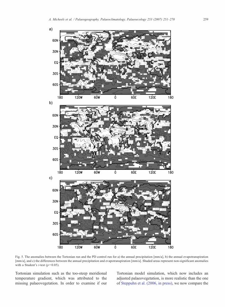
Fig. 5. The anomalies between the Tortonian run and the PD control run for a) the annual precipitation [mm/a], b) the annual evapotranspiration[mm/a], and c) the differences between the annual precipitation and evapotranspiration [mm/a]. Shaded areas represent non-significant anomalieswith a Student's t-test (p=0.05).
259A. Micheels et al. / Palaeogeography, Palaeoclimatology, Palaeoecology 253 (2007) 251–270
Tortonian simulation such as the too-steep meridionaltemperature gradient, which was attributed to themissing palaeovegetation. In order to examine if our
Tortonian model simulation, which now includes anadjusted palaeovegetation, is more realistic than the oneof Steppuhn et al. (2006, in press), we now compare the
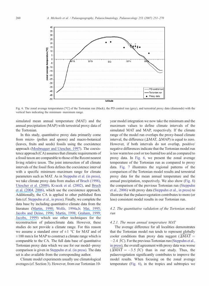
Fig. 6. The zonal average temperatures [°C] of the Tortonian run (black), the PD control run (grey), and terrestrial proxy data (diamonds) with thevertical bars indicating the minimum–maximum range.
260 A. Micheels et al. / Palaeogeography, Palaeoclimatology, Palaeoecology 253 (2007) 251–270
simulated mean annual temperature (MAT) and theannual precipitation (MAP) with terrestrial proxy data ofthe Tortonian.
In this study, quantitative proxy data primarily comefrom micro- (pollen and spores) and macro-botanical(leaves, fruits and seeds) fossils using the coexistenceapproach (Mosbrugger and Utescher, 1997). The coexis-tence approach (CA) assumes that climatic requirements ofa fossil taxon are comparable to those of the Recent nearestliving relative taxon. The joint intersection of all climateintervals of the fossil flora defines the coexistence intervalwith a specific minimum–maximum range for climateparameters such as MAT. As in Steppuhn et al. (in press),we take climate proxy data from studies of Bruch (1998),Utescher et al. (2000), Kvacek et al. (2002), and Bruchet al. (2004, 2006), which use the coexistence approach.Additionally, the CA is applied to other published floralists (cf. Steppuhn et al., in press). Finally, we complete thedata base by including quantitative climate data from theliterature (Martin, 1990; Wolfe, 1994a,b; Mai, 1995;Jacobs and Deino, 1996; Martin, 1998; Graham, 1999;Jacobs, 1999) which use other techniques for thereconstruction of palaeoclimate data. However, thesestudies do not provide a climate range. For this reasonwe assume a standard error of ±1 °C for MAT and of±100 mm/a for MAP to construct a climate range which iscomparable to the CA. The full data base of quantitativeTortonian proxy data which we use for our model–proxycomparison is given in Steppuhn et al. (in press). The dataset is also available from the corresponding author.
Climate model experiments usually use climatologicalaverages (cf. Section 3). However, from our Tortonian 10-
year model integration we now take the minimum and themaximum values to define climate intervals of thesimulated MAT and MAP, respectively. If the climaterange of the model run overlaps the proxy-based climateinterval, the difference (ΔMAT, ΔMAP) is equal to zero.However, if both intervals do not overlap, positive/negative differences indicate that the Tortonian model runis too warm/too cool or too humid/too arid as compared toproxy data. In Fig. 6, we present the zonal averagetemperature of the Tortonian run as compared to proxydata. Fig. 7 illustrates the regional patterns of thecomparison of the Tortonian model results and terrestrialproxy data for the mean annual temperature and theannual precipitation, respectively. We also show (Fig. 8)the comparison of the previous Tortonian run (Steppuhnet al., 2006) with proxy data (Steppuhn et al., in press) toillustrate that the palaeovegetation contributes to more (orless) consistent model results in our Tortonian run.
4.2. The quantitative validation of the Tortonian modelrun
4.2.1. The mean annual temperature MATThe average difference for all localities demonstrates
that the Tortonian model run tends to represent globallycooler conditions than proxy data suggest (
PDMAT ¼
�2:4 -C). For the previousTortonian run (Steppuhn et al.,in press), the overall agreement with proxy data wasworse(PDMAT ¼ �3:5 -C) than in our study. Thus, thepalaeovegetation significantly contributes to improve themodel results. When focusing on the zonal averagetemperature (Fig. 6), in the tropics and subtropics we
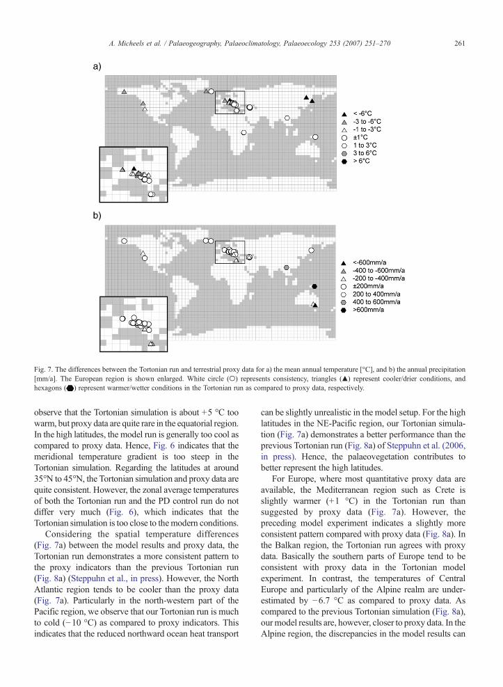
Fig. 7. The differences between the Tortonian run and terrestrial proxy data for a) the mean annual temperature [°C], and b) the annual precipitation[mm/a]. The European region is shown enlarged. White circle (○) represents consistency, triangles (▴) represent cooler/drier conditions, andhexagons ( ) represent warmer/wetter conditions in the Tortonian run as compared to proxy data, respectively.
261A. Micheels et al. / Palaeogeography, Palaeoclimatology, Palaeoecology 253 (2007) 251–270
observe that the Tortonian simulation is about +5 °C toowarm, but proxy data are quite rare in the equatorial region.In the high latitudes, the model run is generally too cool ascompared to proxy data. Hence, Fig. 6 indicates that themeridional temperature gradient is too steep in theTortonian simulation. Regarding the latitudes at around35°N to 45°N, the Tortonian simulation and proxy data arequite consistent. However, the zonal average temperaturesof both the Tortonian run and the PD control run do notdiffer very much (Fig. 6), which indicates that theTortonian simulation is too close to themodern conditions.
Considering the spatial temperature differences(Fig. 7a) between the model results and proxy data, theTortonian run demonstrates a more consistent pattern tothe proxy indicators than the previous Tortonian run(Fig. 8a) (Steppuhn et al., in press). However, the NorthAtlantic region tends to be cooler than the proxy data(Fig. 7a). Particularly in the north-western part of thePacific region, we observe that our Tortonian run is muchto cold (−10 °C) as compared to proxy indicators. Thisindicates that the reduced northward ocean heat transport
can be slightly unrealistic in the model setup. For the highlatitudes in the NE-Pacific region, our Tortonian simula-tion (Fig. 7a) demonstrates a better performance than theprevious Tortonian run (Fig. 8a) of Steppuhn et al. (2006,in press). Hence, the palaeovegetation contributes tobetter represent the high latitudes.
For Europe, where most quantitative proxy data areavailable, the Mediterranean region such as Crete isslightly warmer (+1 °C) in the Tortonian run thansuggested by proxy data (Fig. 7a). However, thepreceding model experiment indicates a slightly moreconsistent pattern compared with proxy data (Fig. 8a). Inthe Balkan region, the Tortonian run agrees with proxydata. Basically the southern parts of Europe tend to beconsistent with proxy data in the Tortonian modelexperiment. In contrast, the temperatures of CentralEurope and particularly of the Alpine realm are under-estimated by −6.7 °C as compared to proxy data. Ascompared to the previous Tortonian simulation (Fig. 8a),ourmodel results are, however, closer to proxy data. In theAlpine region, the discrepancies in the model results can
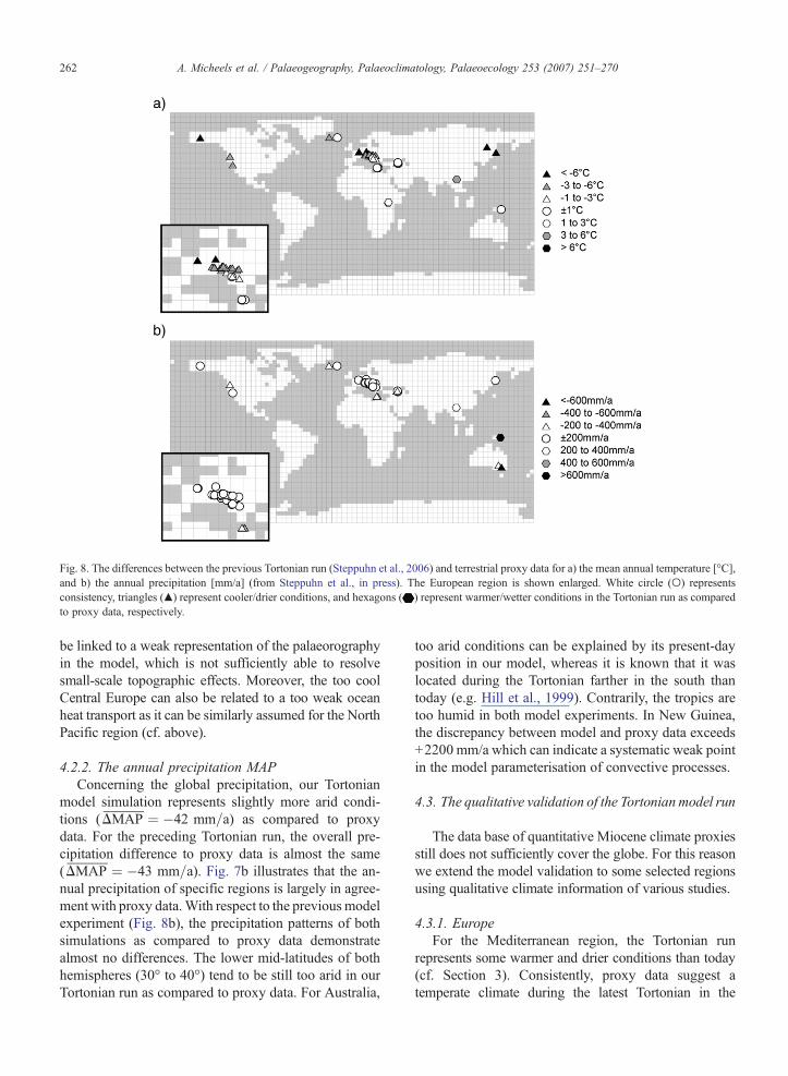
Fig. 8. The differences between the previous Tortonian run (Steppuhn et al., 2006) and terrestrial proxy data for a) the mean annual temperature [°C],and b) the annual precipitation [mm/a] (from Steppuhn et al., in press). The European region is shown enlarged. White circle (○) representsconsistency, triangles (▴) represent cooler/drier conditions, and hexagons ( ) represent warmer/wetter conditions in the Tortonian run as comparedto proxy data, respectively.
262 A. Micheels et al. / Palaeogeography, Palaeoclimatology, Palaeoecology 253 (2007) 251–270
be linked to a weak representation of the palaeorographyin the model, which is not sufficiently able to resolvesmall-scale topographic effects. Moreover, the too coolCentral Europe can also be related to a too weak oceanheat transport as it can be similarly assumed for the NorthPacific region (cf. above).
4.2.2. The annual precipitation MAPConcerning the global precipitation, our Tortonian
model simulation represents slightly more arid condi-tions (PDMAP ¼ �42 mm=a) as compared to proxy
data. For the preceding Tortonian run, the overall pre-cipitation difference to proxy data is almost the same(PDMAP ¼ �43 mm=a). Fig. 7b illustrates that the an-nual precipitation of specific regions is largely in agree-ment with proxy data.With respect to the previous modelexperiment (Fig. 8b), the precipitation patterns of bothsimulations as compared to proxy data demonstratealmost no differences. The lower mid-latitudes of bothhemispheres (30° to 40°) tend to be still too arid in ourTortonian run as compared to proxy data. For Australia,
too arid conditions can be explained by its present-dayposition in our model, whereas it is known that it waslocated during the Tortonian farther in the south thantoday (e.g. Hill et al., 1999). Contrarily, the tropics aretoo humid in both model experiments. In New Guinea,the discrepancy between model and proxy data exceeds+2200 mm/a which can indicate a systematic weak pointin the model parameterisation of convective processes.
4.3. The qualitative validation of the Tortonian model run
The data base of quantitative Miocene climate proxiesstill does not sufficiently cover the globe. For this reasonwe extend the model validation to some selected regionsusing qualitative climate information of various studies.
4.3.1. EuropeFor the Mediterranean region, the Tortonian run
represents some warmer and drier conditions than today(cf. Section 3). Consistently, proxy data suggest atemperate climate during the latest Tortonian in the

263A. Micheels et al. / Palaeogeography, Palaeoclimatology, Palaeoecology 253 (2007) 251–270
south of the Iberian Peninsula (Brachert et al., 1996).During the Late Miocene, the north-eastern part of Spainis a transitional region from a temperate humid to a sub-tropical dry climate (Alonzo-Zarza and Calvo, 2000). Forcentral and northern Italy during the Late Tortonian,Bertini (1994) found indications of subtropical to warmtemperate conditions which shift to a warm temperateclimate during the Zanclean. Before 10.5 and after8.5 Ma, fossil small mammals from Spain indicate morearid and warmer conditions (van Dam and Weltje, 1999).This is consistent with the Tortonian model simulation.However, Spain is more humid and cooler between 10.5and 8.5Ma (van Dam andWeltje, 1999) which tends to bea conflict with the model run.
For Central Europe, the Tortonian run indicates aclimate which is almost as warm as today but more humid(cf. Section 3). During the Late Miocene a transition froma warm and dry Southern European climate to a wet–dryseasonal climate inNorthern Europe occurs (vanDam andWeltje, 1999), which agrees with the Tortonian run. Forthe European realm, the comparison of model results andproxy data indicates that the Tortonian model experimenttends to better represent the late Tortonian than the earlypart.
4.3.2. North AmericaFor the mid-latitudes of the North American conti-
nent, the Tortonian run represents almost the same meanannual temperature than today but rainfalls are higher(cf. Section 3). The mammal fauna of North America(Fox, 2000) indicates a change from a low seasonal EarlyMiocene climate towards a more highly seasonal climateduring the Late Miocene. Fox (2000) demonstrated anincrease in aridity in North America during the LateMiocene with a distinct wet season. This pattern is notobserved in our Tortonian run. For the east coast of NorthAmerica during the Late Miocene, the climate was inter-mediate between warm temperate and cool temperateconditions (McCartan et al., 1990). The absence of sub-tropical evergreen elements for this LateMiocene localitycan hint on Arctic cold fronts and, hence, on similar-to-present climate conditions in the eastern part of NorthAmerica. This qualitatively agrees with the Tortonian run.Since the end of the Middle Miocene the summer tem-peratures of North America decrease (Wolfe, 1994a) andcoastal regions of western North America at around13Ma indicate some higher MATs than the interior of theNorth American continent (Wolfe, 1994a). Basically thisis consistent with the Tortonian run.
In the high latitudes, generally warmer climaticconditions are observed in our Tortonian run as comparedto the PD control run (cf. Section 3). However, these
temperatures are still lower than proxy data suggest (cf.Section 4.2). From 12 to 8 Ma, temperatures decline inAlaska (Wolfe, 1994b). During this period, the decreasingsummer temperatures in the Alaska region are moreaffected than the winter temperatures (Wolfe, 1994b). Atabout 6 to 5 Ma, the Alaska summer temperatures arealmost the same as today (Wolfe, 1994b). For Canada andAlaska between 9.7 and 5.7 Ma, White et al. (1997)suggest a cooling trend. In Beringia, the Late Miocenemean annual temperatures are +2 °C to +4 °C higher thannowadays (Wolfe, 1994b). This temperature difference isconsistent with the difference between the Tortonian andthe Recent Control run (cf. Section 3).
4.3.3. AsiaIn the Tortonian model experiment the Asian summer
monsoon tends to be weaker than today representingwarmer andmore arid conditions in southern parts of Asia.Primarily the lower elevation of the Miocene TibetanPlateau causes the overall weakening of the monsoon(Steppuhn et al., 2006). Consistent with a weak Miocenemonsoon in our model run, Griffin (2002) suggested thatthe Asian monsoon began at 8 to 7 Ma, and Wang et al.(1999) concluded that the Asian monsoon intensified at8 to 7 Ma which led to a drying of the Quaidam Basin andnorthern Pakistan. Our Tortonian run represents a weakerthan present monsoon, but the palaeovegetation partlycontributes to strengthen the Asian monsoon rainfallsduring the summer season. Sakai (1997) consistentlyreported that the Asian summer monsoon existed prior to10 Ma. Moreover, Ding et al. (1999) found that thesummer monsoon was possibly stronger than during theHolocene. Our Tortonian model simulations indicate thatthis observation can be attributed to the palaeovegetation.Overall, the Asian monsoon in the Tortonian run isqualitatively consistent with proxy data.
4.3.4. South AmericaFor South America, the Tortonian run suggests slightly
warmer and more humid conditions than today (cf.Section 3). δ13C values of fossil mammal teeth from theBolivian Andes at around 10 Ma give evidence ofwidespread grasslands with temperate or even tropicalelements (MacFadden et al., 1994). In the Central Andesat the same time, the terrigenous influx to the Amazon fanincreased (Gregory-Wodzicki, 2000) which correspondsto higher rainfalls in this region as also represented in theTortonian run (cf. Section 3). Seasonally dry forests grewin the Ecuadorian Andes at around 13 to 10Ma (Burnhamand Carranco, 2004), but this does not fit with the higherprecipitation rate in the Tortonian run. For the AtacamaDesert between 14.7 and 8.7 Ma, proxy data indicate an
264 A. Micheels et al. / Palaeogeography, Palaeoclimatology, Palaeoecology 253 (2007) 251–270
onset of aridity with a transition to hyperarid conditions(Gregory-Wodzicki, 2000). Such arid conditions areconsistently illustrated from the Tortonian run.
4.3.5. AustraliaAustralia is almost as warm as today in the Tortonian
simulation (cf. Section 3). The model experiment alsodemonstrates higher rainfall rates than today, but themodel represents still too dry conditions as compared tosouthern Australian quantitative proxy data (cf. Section4.2). Late Miocene carbonate deposits at the north-eastof Australia indicate non-tropical conditions (Betzler,1997). For north-east Australia, Betzler et al. (1995)proposed surface water temperatures of about 17 °C to19 °C from the absence of coral reef growth. Inconsistentwith these proxy data, we do not observe these coolerconditions from the Tortonian model simulation. Tooarid and too cool conditions in our model run can berelated to the present-day palaeogeography in our modelrun which does not consider that Australia was locatedfarther southward in the Miocene (e.g. Hill et al., 1999).
4.3.6. The Northern Hemisphere's ice coverOn the Northern Hemisphere, the Tortonian run
demonstrates a lower amount of sea ice as compared tothe PD control run (cf. Section 3). Consistently, Mioceneproxy data indicate that the Arctic sea ice volume is lessthan today (Wolf and Thiede, 1991), but so far detailedinformation about the Miocene Arctic ice cover does notexist (Schaeffer and Spiegler, 1986; Thiede et al., 1998).During the Late Pliocene (3.5 to 2.4 Ma), a successiveonset of a large-scale glaciation of the Atlantic Oceanoccurred (Kleiven et al., 2002). However, Helland andHolmes (1997) found indications that the North Atlanticand Greenland glaciation began earlier at around 11 Ma,which is consistent with the presence of sea icethroughout the year in the Tortonian run. Moran et al.(2006) recently published that there is evidence for (atleast seasonal) sea ice in the Arctic Ocean at 14 Ma. Thisstudy also generally supports results of our Tortonianrun. However, the validation with terrestrial proxy dataindicates that the model run is too cool in higher latitudes(cf. above). For this reason, the Arctic sea ice cover canstill be overestimated in the model simulation.
5. Discussion
In order to better understand the Tortonian climate,we present a Tortonian simulation with the highlycomplex atmospheric general circulation modelECHAM4/ML. Generally climate models include somesystematic weak points. In the ECHAM model, e.g. the
vegetation is parameterised as a non-dynamical system(e.g. Roeckner et al., 1992, 1996). Despite some weakpoints, the ECHAMmodel, however, shows a quite goodperformance when applied to the present-day situationand to the Quaternary (e.g. Latif and Neelin, 1994;Lorenz et al., 1996; Montoya et al., 1998).
Our study is based on a preceding Tortonianmodel run(Steppuhn et al., 2006) which used a weaker than presentpalaeocean heat transport and a lower palaeoelevation. Inaddition, our Tortonian model experiment includes anappropriate palaeovegetation (Micheels, 2003). From ourTortonian run, we observe a polar warming which isattributed to the lower Greenland elevation and to theeffects of the palaeovegetation. Basically these resultscorrespond to other Miocene modelling studies (e.g.Dutton and Barron, 1997; Kutzbach and Behling, 2004).In an Early Miocene sensitivity experiment, Dutton andBarron (1997) found that the higher forest cover ascompared to today caused polar warming and this reducedthe meridional temperature gradient. This was not shownin Steppuhn et al.'s (2006) Tortonian run, but fits with ourmodel run. With respect to the lower Tibetan Plateauduring the Miocene, the Tortonian run demonstrates aweaker than present Asian monsoon. Consistent with ourstudy, AGCM sensitivity experiments address thestrengthening of the Asian monsoon during the last30Ma to the uplift of the Tibetan Plateau (Ramstein et al.,1997; Fluteau et al., 1999). We thus claim that theTortonian run generally agrees with results of previousMiocene model experiments.
In order to analyse if our Tortonian modelling resultsfit not only with other model data but are also consistentwith the fossil record, we quantitatively compare theresults of the Tortonian run with climate proxy data.However, the poor Miocene data base (Mosbrugger andSchilling, 1992) is a major problem for validating modelresults. For many parts of the globe, quantitativeTortonian proxy data are still not sufficiently availableand hence model results can be validated only for selectedregions. However, there remains the question if singleproxy data localities can be representative for a wholemodel grid cell. Due to the limited resolution, climatemodels use parameterisations for small-scale effects suchas the cumulus convection scheme of the ECHAMmodel(Roeckner et al., 1996), which includes some uncertain-ties. In addition, the Tortonian (11 to 7Ma) corresponds toa time span of about 4 million years and the Tortonianmodel run represents an average state over the entireperiod. Due to this integration, it is not trivial to comparemodel results with proxy data. Regarding the palaeocli-mate information, studies can differ as they refer tospecific time intervals within the Tortonian (e.g. van Dam
265A. Micheels et al. / Palaeogeography, Palaeoclimatology, Palaeoecology 253 (2007) 251–270
and Weltje, 1999). For instance, an eastern Icelandlocality, which is dated between 10.3 and 9.5 Ma(Mudie and Helgason, 1983), tends to be consistent tothe Tortonian run. Contrarily a more western Icelandlocality with an age of 11 to 5.3 Ma (Mai, 1995) indicatesa warmer situation than the Tortonian run. With regard toEuropean proxy data (e.g. van Dam andWeltje, 1999) weobserve that the Tortonian run tends to correspond rathermore to the Late Tortonian than to earlier parts of the timeinterval.
Generally, proxy-based methods for climate recon-structions such as CLAMP (Wolfe, 1993) or CA(Mosbrugger and Utescher, 1997) include uncertainties.The CLAMP method is calibrated on climate observa-tions and leaf distributions predominantly from NorthAmerica and Eastern Asia (Wolfe, 1993). However, whenapplied to Miocene floras from Europe (e.g. Mosbruggerand Utescher, 1997; Utescher et al., 2000; Kvacek et al.,2002; Uhl et al., 2006) and even Asia (Liang et al., 2003),the CLAMPmethod produces systematically lower meanannual temperatures than the CA. Nevertheless, for NorthAmerican floras CLAMP achieves reasonable results (e.g.Wolfe, 1993, 1994a) and, if CLAMP underestimates theMAT in this region, the discrepancies between theTortonian run and proxy data would be even greater.
The coexistence approach (Mosbrugger and Utescher,1997) also includes uncertainties. During the Cretaceousor the Eocene the tropics are warmer than present (e.g.Pearson et al., 2001), but modern plant communities canonly represent present-day climatic conditions. From therelationship between modern and fossil plants, it is notpossible to estimate the upper temperature limit of such‘supertropic’ palaeosituations. The CA cannot be appliedto situations whose conditions are not found today. But asthe Late Miocene climate is quite similar to the modernsituation (Bruch, 1998), this argument does not apply forthe present study. However, it can be difficult to find anearest living relative and consequently the climateinterval of a particular taxon can be (more or less)incorrect. The CA uses the joint intersection interval of alltaxa, which keeps single errors small. The CA demon-strates its capability for palaeoclimate reconstructions forthe European and Asian Neogene (Utescher et al., 1997;Bruch, 1998; Utescher et al., 2000; Bruch and Mos-brugger, 2002; Kvacek et al., 2002; Liang et al., 2003; Uhlet al., 2003).
Despite shortcomings of different techniques, themethods used here for the quantitative estimation ofpalaeoclimate data produce quite consistent patterns (e.g.Wolfe, 1994a,b; Kvacek et al., 2002; Liang et al., 2003;Uhl et al., 2003). For this reason they offer the possibilityto test the reliability of model results. When compared to
proxy data, our Tortonian run demonstrates more realisticresults than the preceding Tortonian run of Steppuhn et al.(2006, in press). For instance, on the global scale ourTortonian run is −2.4 °C too cool as compared to proxydata, whereas Steppuhn et al.'s (2006, in press) Tortonianrun demonstrates a difference of −3.5 °C. Thus, thepalaeovegetation significantly contributes to improve-ment of the model results.
Nevertheless, there still remain some discrepanciesbetween our Tortonian run and proxy data. Our Tortoniansimulation tends to be too cool in the high latitudes and themeridional temperature gradient is thus not as weak asproxy data suggest (cf. Section 4). However, for Beringiaour Tortonian run presents a temperature difference of+2 °C to +4 °C as compared to the control run (cf. Section3) which is consistently (+2 °C to +4 °C) suggested fromproxy data (Wolfe, 1994b). With respect to the precipi-tation patterns in tropical latitudes, the differences arereasonable between the Tortonian run and the PD controlrun (cf. Section 3), but tropical rainfalls are unrealisticallyhigh as compared to proxy data (cf. Section 4). Fortropical areas, it is already known that the ECHAM4model overestimates precipitation rates as compared topresent-day observation data (Roeckner et al., 1996). Ourstudy indicates that the direct comparison of the Tortonianrun with proxy data is problematic, but climate trends, theTortonian minus control run and proxy data minusmodern observation data, are quite consistent.
Our Tortonian model simulation still demonstratessome discrepancies to proxy data (cf. Section 4) whichcan be explained with weak points in the model setup. Inparticular the model validation demonstrates that theNorth Pacific region tends to be too cool in the Tortonianmodel simulation, whereas the North Atlantic region isquite well represented. This indicates that the adjustedpalaeo-flux correction for the North Pacific can beunrealistic. Focusing on the effects of the closure of theCentral American Isthmus, Mikolajewicz and Crowley(1997) observed that the thermohaline circulation in theNorth Atlantic Ocean was weaker than present which isbasically consistent to our study. However, the sameocean model experiment demonstrated that the NorthPacific surface circulation was almost unaffected by anopenCentral American Isthmus in the LateMiocene. Thismeans that the ocean model represents (more or less) apresent-day northward heat transport in the Pacific Ocean,whereas our prescribed palaeocean heat transport isnoticeably weaker than today. For the high latitudes,almost all oxygen isotope data for the reconstruction ofthe palaeocean heat transport come from the NorthAtlantic region (Steppuhn et al., 2006). The North Pacificis not well represented with δ18O data and due to this lack
266 A. Micheels et al. / Palaeogeography, Palaeoclimatology, Palaeoecology 253 (2007) 251–270
of information Steppuhn et al. (2006) can underestimatethe northward heat transport in the Pacific Ocean. Astrengthened heat transport in the Pacific Ocean, ascompared to the prescribed weakened one, can producesome warmer conditions in the high latitudes of thePacific region than being more consistent to proxy data.
In addition to a possibly unrealistic palaeocean heattransport, the choice of the modern land–sea distributioncan be responsible for discrepancies in the Tortonian run.For the Tortonian model setup we do not consider theParatethys because the method to adjust the fluxcorrection of the slab ocean model does not allowchanging the geography (Steppuhn et al., 2006). Asensitivity experiment of Ramstein et al. (1997), however,demonstrated that the retreat of the Paratethys during theCenozoic led to a cooling in Central Eurasia andparticularly in Siberia. Moreover, the presence of theParatethys contributes to a formerly more humid climatein Eastern Europe (Ramstein et al., 1997). In our modelsetup, we also neglect that the Australian continent wasfarther southward in the Miocene (e.g. Hill et al., 1999).Since the Eocene, Australia shifted northward whichpartly explains the climate change as it is represented inthe fossil record (Martin, 1998; Frakes, 1999; Hill et al.,1999). In the Miocene, Australia was rather more in thetemperate wet zone than near the boundary between thetemperate wet and the tropical dry belt today which canexplain the too arid conditions in our Tortonian run ascompared to proxy data. In particular, model experimentsdemonstrated that both atmospheric and oceanic circula-tions are globally sensitive with respect to the position ofAustralia and the Indonesian Throughflow in theCenozoic (e.g., Cane and Molnar, 2001; Lawver andGahagan, 2003). The Tortonian run includes the effects ofa different-than-present ocean circulation as we use anadjusted Late Miocene flux correction based on δ18Oisotope data (Steppuhn et al., 2006), even though themethod is limited (cf. above). The position of Australia isrelevant for the atmospheric circulation (e.g., Cane andMolnar, 2001). Hence, some discrepancies in ourTortonian simulation can be attributed to an inadequategeography such as the missing Paratethys and the present-day position of Australia in our Tortonian run.
Related to plate tectonicmovements, the LateMioceneorography was different from the modern one (cf.Section 2). Basically, we reduce the palaeoelevation ofthe highmountain ranges such as the Tibetan Plateau. Theestimation of palaeoaltitudes is not trivial (Ruddimanet al., 1997). Several studies analysed the uplift of theTibetan Plateau in the Neogene and gave differentestimations of the elevation of the plateau (e.g. Molnaret al., 1993; Wang et al., 1999). According to Prell and
Kutzbach (1992), we assume that the Tibetan Plateau washalf as high as today. With respect to the southern part ofTibet, it is commonly accepted that it was already at thepresent-day's elevation since 15 Ma (Spicer et al., 2003).This is, however, not represented in ourmodel simulation.On the one hand, the model resolution of 3.75° is toocoarse to resolve a detailed palaeorography. This makes itnecessary to average the palaeotopography over a largerarea. On the other hand, the spectral transformationmethod of the ECHAMmodel (e.g. Roeckner et al., 1992)leads to a slight smoothing effect of smaller-scaleorographic patterns during our model integration. Pri-marily, we prescribed a Late Miocene palaeorographywhich is consistent with other studies (e.g. Ramstein et al.,1997; Kutzbach and Behling, 2004).
We can also address some shortcomings of ourTortonian model experiment to the palaeovegetation.Although the number of localities for which floristicinformation is available is larger than the number oflocalities for which we have quantitative proxy-basedclimate-estimates, we do not have a complete worldwidecoverage of palaeovegetational data (e.g. Mosbruggerand Schilling, 1992; Micheels, 2003). This means thatfor large areas the palaeovegetation has to be interpo-lated based on the available floristic information and thedistribution of modern vegetation. Also a certainamount of time averaging cannot be excluded whichcan also cause some inconsistencies in our palaeovege-tational reconstruction.
To take the palaeovegetation into account in themodel, we adapted the land-surface parameters such asthe leaf area index. However, the surface roughnesslengths remained unchanged and still refer to the present-day vegetation. There are some differences between theTortonian and the modern vegetation, but Dutton andBarron (1996) emphasised that the climatic effects ofvarying roughness lengths due to vegetation changes aregenerally small as compared to the albedo effect and theeffect on the hydrological cycle. In particular the watercycle plays a major role for the climate during the Earth'shistory (Barron et al., 1989). For the ECHAM4 model, asensitivity experiment demonstrates a strong climaticsensitivity on variations of the maximum available soilwater capacity (Kleidon and Heimann, 2000). Thus, theuncertainties of the adapted surface parameters such asthe maximum available soil water capacity are morecrucial than the unchanged roughness length.
In addition, not only the vegetation but also thepalaeorography alter the surface roughness (Claussen,1994). Due to different biome types surface roughnesslengths vary in the order of decimetres (Claussen, 1994),but uncertainties of reconstructed palaeoelevations are
267A. Micheels et al. / Palaeogeography, Palaeoclimatology, Palaeoecology 253 (2007) 251–270
larger. Particularly for mountainous regions vegetation ascompared to orographic changes causes just minorvariations of the surface roughness lengths (Claussen,1994). An unrealistic representation of the climate in ourTortonian run can be attributed rather more to uncertain-ties in the palaeorography than to the unchanged vege-tation roughness lengths.
6. Summary and conclusions
For the Tortonian we perform a model simulation withthe AGCM ECHAM4 coupled to a slab ocean model. Forthe model setup we consider a generally weakerpalaeocean heat transport and a lower palaeorographywhich are based on Steppuhn et al. (2006). In addition toSteppuhn et al. (2006), which included the present-dayvegetation, we use a proxy-based reconstruction of thepalaeovegetation to adapt the surface parameters(Micheels, 2003). The land–sea distribution and theatmospheric CO2 (=353 ppm) refer to present-dayconditions.
The Tortonian run is globally +0.6 °C warmer andthe global precipitation is higher by +27 mm/a than thePD control experiment. On the global scale thepalaeovegetation significantly contributes to the warmer(+0.9 °C) and more humid (+36 mm/a) conditions in theTortonian run. As compared to today, the zonal averagetemperature increases particularly in the northern highlatitudes (+3.5 °C), whereas equatorial regions are justslightly warmer (+0.8 °C) and the Southern Hemisphereis almost as warm as today. In the Northern Hemispherethe Tortonian run hence demonstrates a weaker thanpresent meridional temperature gradient. The polarwarming also tends to reduce the Arctic sea ice cover,but the Tortonian run indicates sea ice cover throughoutthe year.
On the regional scale, the lower altitudes of Green-land and the Tibetan Plateau cause mean annualtemperatures being higher by about +20 °C. In thehigh northern latitudes, the boreal palaeoforests ascompared to the modern tundra vegetation significantlycontribute to warm polar regions (up to +4 °C) and toreduce the meridional temperature gradient in theTortonian run. The lower palaeoelevation of the TibetanPlateau weakens the Asian monsoon as compared totoday. The palaeovegetation tends to strengthen themonsoon during the summer months, but the Asianmonsoon is still weaker than today in the Tortonian run.For Europe, the weak palaeocean heat transport leads toa cooling effect which is partly compensated by thepalaeovegetation. In the Tortonian simulation Europe ishence almost as warm as today.
From the Tortonian run we observe an enhancedhydrological cycle as compared to the PD control run.The precipitation in the Tortonian run increases primar-ily over continental areas, whereas over ocean surfacesconditions tend to be more arid than today. For NorthAfrica, the annual rainfall is by about +500 mm/a higherin the Tortonian run, and +400 mm/a can be attributedto the replacement of the modern Sahara desert withtropical savannas and grassland vegetation during theTortonian. Over continental regions in the northern highand mid-latitudes, the precipitation rates increase by upto +200 mm/a as compared to today. About the half(+50 to +100 mm/a) of the more humid conditions inthe Tortonian run can be ascribed to the larger forestcover in the Tortonian.
We quantitatively compare the model results withterrestrial proxy data. Basically the Tortonian run isconsistent with proxy data, but there are also somediscrepancies. The average for all proxy data localitiesindicates that the Tortonian run tends to be too cool andtoo dry as compared to the fossil record. The modelsimulation is too cool primarily in the high latitudes andthus the meridional temperature gradient in theTortonian run is still not as weak as proxy data suggest.In the North Pacific region, the comparison of modelresults and proxy data indicates that the adjusted palaeo-flux correction of the mixed-layer ocean model canrepresent a too weak northward ocean heat transport.For Southern Europe, the Tortonian run is consistentwith proxy data, but for the Alpine region proxy datasuggest a warmer climate than the model experiment.However, the too-cool conditions in the model runcan be attributed to small-scale orographic effects whichcannot be resolved with the coarse model grid.With respect to precipitation patterns, there is an overallquite good agreement between model results andproxy data. Just in the tropics, we identify that theTortonian simulation overestimates the annual rainfallby far (+2200 mm/a) which can be addressed to theparameterisation of the cumulus convection scheme ofECHAM.
As compared to the preceding Tortonian study ofSteppuhn et al. (2006, in press) which includes themodern vegetation, our Tortonian run is more realistic.However, the discrepancies in our Tortonian run demon-strate that we still do not fully understand the LateMiocene.We cannot yet sufficiently explain why the highlatitudes are warmer and why the meridional temperaturegradient is weak during the Miocene. In addition to thehitherto existing Miocene climate modelling conceptswith AGCMs using either palaeo-SSTs or a simple slabocean model, we suggest to complete the model hierarchy
268 A. Micheels et al. / Palaeogeography, Palaeoclimatology, Palaeoecology 253 (2007) 251–270
with fully coupled atmosphere–ocean general circulationmodels.
Acknowledgements
The present work is a contribution to the NECLIMEframework. We would like to thank the DeutscheForschungsgemeinschaft (DFG) for their financialsupport. The model ECHAM4/ML was kindly providedfrom the Max-Planck Institute of Meteorology, Ham-burg. The computer simulations were performed at theDeutsches Klimarechenzentrum DKRZ, Hamburg. Wealso thank the reviewers M. Böhme, J. Parrish and G.Upchurch for their helpful comments and suggestionswhich contributed to improve our manuscript.
References
Alonzo-Zarza, A.M., Calvo, J.P., 2000. Palustrine sedimentation in anepisodically subsiding basin: the Miocene of the northern TeruelGraben (Spain). Palaeogeography, Palaeoclimatology, Palaeoecol-ogy 160, 1–21.
Barron, E.J., Hay, W.W., Thompson, S., 1989. The hydrological cycle:a major variable during Earth history. Palaeogeography, Palaeo-climatology, Palaeoecology 75, 157–174.
Bertini, A., 1994. Palynological investigations on Upper Neogene andLower Pleistocene sections in central and northern Italy. Memoriedella Societa Geologica Italiana 48, 431–443.
Betzler, C., 1997. Ecological controls on geometries of carbonateplatforms: Miocene/Pliocene shallow-water microfaunas andcarbonate biofacies from the Queensland Plateau (NE Australia).Facies 37, 147–166.
Betzler, C., Brachert, T.C., Kroon, D., 1995. Role of climate in partialdrowning of the Queensland Plateau carbonate platform (north-eastern Australia). Marine Geology 123, 11–32.
Brachert, T.C., Betzler, C., Braga, J.C., Martin, J.M., 1996. Record ofclimatic change in neritic carbonates: turnover in biogenicassociations and depositional modes (Late Miocene, southernSpain). Geologische Rundschau 85, 327–337.
Bruch, A.A., 1998. Palynologische Untersuchungen im OligozänSloweniens — Paläo-Umwelt und Paläoklima im Ostalpenraum.Tübinger Mikropaläontologische 18.
Bruch, A.A., Mosbrugger, V., 2002. Palaeoclimate versus vegetationreconstruction — palynological investigations on the Oligocenesequence of the Sava Basin, Slovenia. Review of Palaeobotany andPalynology 122, 117–141.
Bruch, A.A., Utescher, T., Alcalde Olivares, C., Dolakova, N.,Mosbrugger, V., 2004. Middle and Late Miocene spatialtemperature patterns and gradients in Central Europe —preliminary results based on palaeobotanical climate reconstruc-tions. Courier Forschungsinstitut Senckenberg 249, 15–27.
Bruch, A.A., Utescher, T., Mosbrugger, V., Gabrielyan, I., Ivanov, D.A.,2006. Late Miocene climate in the circum-Alpine realm—aquantitative analysis of terrestrial palaeofloras. Palaeogeography,Palaeoclimatology, Palaeoecology 238, 270–280.
Burnham, R.J., Carranco, N.L., 2004. Miocene winged fruits of Lox-opterygium (Anacardiaceae) from the Ecuadorian Andes. Amer-ican Journal of Botany 91, 1767–1773.
Cane, M.A., Molnar, P., 2001. Closing of the Indonesian seaway as aprecursor to east African aridification around 3–4 million yearsago. Nature 411, 157–162.
Claussen, M., 1994. On coupling global biome models with climatemodels. Max-Planck-Institut für Meteorologie, Hamburg, Report131.
Crowley, T.J., Zachos, J.C., 2000. Comparison of zonal temperatureprofiles for past warm time periods. In: Huber, B.T., MacLeod, K.G.,Wing, S.L. (Eds.), Warm Climates in Earth History. CambridgeUniversity Press, Cambridge. 462 pp.
Ding, Z.L., Xiong, S.F., Sun, J.M., Yang, S.L., Gu, Z.Y., Liu, T.S.,1999. Pedostratigraphy and paleomagnetism of a approximately 7.0Ma eolian loess-red clay sequence at Lingtai, Loess Plateau, north-central China and the implications for paleomonsoon evolution.Palaeogeography, Palaeoclimatology, Palaeoecology 152, 49–66.
DKRZ Modellbetreuungsgruppe, 1994. The ECHAM3 atmosphericgeneral circulation model. Technical Report, vol. 6. DeutschesKlimarechenzentrum, Hamburg.
DKRZ Modellbetreuungsgruppe, 1997. ECHAM4 — WorkshopHamburg, November 25th 1996. Deutsches Klimarechenzentrum,Hamburg.
Dutton, J.F., Barron, E.J., 1996. Genesis sensitivity to changes in pastvegetation. Palaeoclimates 1, 325–354.
Dutton, J.F., Barron, E.J., 1997. Miocene to present vegetationchanges: a possible piece of the Cenozoic puzzle. Geology 25 (1),39–41.
Fluteau, F., Ramstein, G., Besse, J., 1999. Simulating the evolution ofthe Asian and African monsoons during the past 30 Myr using anatmospheric general circulation model. Journal of GeophysicalResearch 104, 11995–12018.
Fox, D.L., 2000. Growth increments in Gomphotherium tusks andimplications for the Late Miocene climate change in North America.Palaeogeography, Palaeoclimatology, Palaeoecology 156, 327–348.
Frakes, L.A., 1999. Evolution of Australian environments, In:Orchard, A.E. (Ed.), 2nd edition. Flora of Australia, vol. 1.ABRS/CSIRO, Canberra, pp. 163–203.
Graham, A., 1999. Late Cretaceous and Cenozoic History of NorthAmerican Vegetation North of Mexico. Oxford University Press.370 pp.
Gregory-Wodzicki, K.M., 2000. Uplift history of the Central andNorthern Andes: a review. Geological Society of America Bulletin112 (7), 1091–1105.
Griffin, D.L., 2002. Aridity and humidity: two aspects of the lateMiocene climate of North Africa and the Mediterranean.Palaeogeography, Palaeoclimatology, Palaeoecology 182, 65–91.
Heer, O., 1859. Flora Tertiara Helvetiae III. Verlag von Wurster undComp., Winterthur. 378 pp.
Heer, O., 1868. Flora fossilis Arctica 1. Die fossile Flora derPolarländer enthaltend die in Nordgrönland, auf der Melville-Insel, im Banksland, am Mackenzie. Island und in Spitzbergenentdeckten fossilen Pflanzen. Zürich. 192 pp.
Helland, P.E., Holmes, M.A., 1997. Surface textural analysis of quartzsand grains from ODP Site 918 off the southeast coast of Greenlandsuggests glaciation of southern Greenland at 11 Ma. Palaeogeo-graphy, Palaeoclimatology, Palaeoecology 135, 109–121.
Hill, R.S., Truswell, E.M., McLoughlin, S., Dettmann, M.E., 1999.The evolution of the Australian flora: fossil evidence, In: Orchard,A.E. (Ed.), 2nd edition. Flora of Australia, vol. 1. ABRS/CSIRO,Canberra, pp. 163–203.
Jacobs, B.F., 1999. Estimation of rainfall variables from leaf charactersin tropical Africa. Palaeogeography, Palaeoclimatology, Palaeoe-cology 145, 231–250.

269A. Micheels et al. / Palaeogeography, Palaeoclimatology, Palaeoecology 253 (2007) 251–270
Jacobs, B.F., Deino, A.L., 1996. Test of climate–leaf physiognomyregression models, their application to two Miocene floras fromKenya, and 40Ar/39Ar dating of the Late Miocene Kapturo site.Palaeogeography, Paleoclimatology, Palaeoecology 123, 259–271.
Kim, S.J., Crowley, T.J., 2000. Increased Pliocene North Atlantic deepwater: cause or consequence of Pliocene warming? Paleoceano-graphy 15, 451–455.
Kleidon, A., Heimann, M., 2000. Assessing the role of deep rootedvegetation in the climate system with model simulations:mechanisms, comparison to observations and implications forAmazonian deforestation. Climate Dynamics 16, 183–199.
Kleiven, H.F., Jansen, E., Fronval, T., Smith, T.M., 2002. Intensifi-cation of Northern Hemisphere glaciations in the circum Atlanticregion (3.5–2.4 Ma); ice-rafted detritus evidence. Palaeogeogra-phy, Palaeoclimatology, Palaeoecology 184, 213–223.
Kutzbach, J.E., Behling, P., 2004. Comparison of simulated changes ofclimate in Asia for two scenarios: Early Miocene to present, andpresent to future enhanced greenhouse. Global and PlanetaryChange 41, 157–165.
Kvacek, Z., Velitzelos, D., Velitzelos, E., 2002. Late Miocene Flora ofVegoraMacedonia N. Greece. University of Athens, Athens. 175 pp.
Latif, M., Neelin, J.D., 1994. El Niño/Southern Oscillation. Report,vol. 129. Max-Planck-Institut für Meteorologie, Hamburg.
Lawver, L.A., Gahagan, L.M., 2003. Evolution of Cenozoic seawaysin the circum-Antarctic region. Palaeogeography, Palaeoclimatol-ogy, Palaeoecology 198, 11–37.
Le Houerou, H.N., 1997. Climate, flora and fauna changes in theSahara over the past 500 million years. Journal of AridEnvironments 37, 619–647.
Liang, M.-M., Bruch, A., Collinson, M., Mosbrugger, V., Li, Ch.-S.,Sun, Q.-G., Hilton, J., 2003. Testing the climatic estimates fromdifferent palaeobotanical methods: an example from the MiddleMiocene Shangwang flora of China. Palaeogeography, Palaeocli-matology, Palaeoecology 198, 279–301.
Lorenz, S., Grieger, B., Helbig, P., Herterich, K., 1996. Investigatingthe sensitivity of the atmospheric general circulation modelECHAM3 to palaeoclimatic boundary conditions. GeologischeRundschau 85 (3), 513–524.
MacFadden, B.J., Wang, Y., Cerling, T.E., Anaya, F., 1994. SouthAmerican fossil mammals and carbon isotopes: a 25 million yearsequence from the Bolivian Andes. Palaeogeography, Palaeocli-matology, Palaeoecology 107, 257–268.
Mai, H.D., 1995. Tertiäre Vegetationsgeschichte Europas: Methodenund Ergebnisse. G. Fischer, Jena, p. 476.
Maier-Reimer, E., Mikolajewicz, U., Crowley, T.J., 1990. Oceangeneral circulation model sensitivity experiment with an openCentral American Isthmus. Palaeoceanography 5 (3), 349–366.
Martin, H.A., 1990. Tertiary climate and phytogeography in southeasternAustralia. Review of Palaeobotany and Palynology 65, 47–55.
Martin, H.A., 1998. Tertiary climatic evolution and the development ofaridity in Australia. Proceedings of the Linnean Society of NewSouth Wales 119, 115–136.
McCartan, L., Tiffney, B.H., Wolfe, J.A., Ager, T.A., Wing, S.L.,Sirkin, L.A., Ward, L.W., Brooks, J., 1990. Late Tertiary floralassemblage from upland gravel deposits of the southern MarylandCoastal Plain. Geology 18, 311–314.
Micheels, A., 2003. Late Miocene climate modelling with ECHAM4/ML— the effects of the palaeovegetation on the Tortonian climate.PhD Thesis, University of Tübingen.
Mikolajewicz, U., Crowley, T.J., 1997. Response of a coupled ocean/energy balance model to restricted flow through the centralAmerican isthmus. Palaeoceanography 12 (3), 429–441.
Mikolajewicz, U., Maier-Reimer, E., Crowley, T.J., Kim, K.J., 1993.Effect of Drake and Panamanian gateways on the circulation of anocean model. Paleoceanography 8 (4), 409–426.
Molnar, P., England, P., Martinod, J., 1993. Mantle dynamics, uplift ofthe Tibetan Plateau and the Indian monsoon. Reviews ofGeophysics 31 (4), 357–396.
Montoya, M., Crowley, T.J., von Storch, H., 1998. Temperatures at thelast interglacial simulated by a coupled ocean–atmosphere climatemodel. Paleoceanography 13 (2), 170–177.
Moran, K., Backman, J., Brinkhuis, H., Clemens, S.C., Cronin, T.,Dickens, G.R., Eynaud, F., Gattacceca, J., Jakobsson, M., Jordan,R.W., Kaminski, M., King, J., Koc, N., Krylov, A., Martinez, N.,Matthiessen, J., McInroy, D., Moore, T.C., Onodera, J., O'Regan,M., Pälike, H., Rea, B., Rio, D., Sakamoto, T., Smith, D.C., Stein,R., St John, K., Suto, I., Suzuki, N., Takahashi, K., Watanabe, M.,Yamamoto, M., Farrell, J., Frank, M., Kubik, P., Jokat, W.,Kristoffersen, Y., 2006. The Cenozoic palaeoenvironment of theArctic Ocean. Nature 441, 601–605.
Mosbrugger, V., Schilling, H.-D., 1992. Terrestrial palaeoclimatologyin the Tertiary: a methodological critique. Palaeogeography,Palaeoclimatology, Palaeoecology 99, 17–29.
Mosbrugger, V., Utescher, T., 1997. The coexistence approach — amethod for quantitative reconstructions of Tertiary terrestrialpalaeoclimate data using plant fossils. Palaeogeography, Palaeo-climatology, Palaeoecology 134, 61–86.
Mudie, P.J., Helgason, J., 1983. Palynological evidence for Mioceneclimatic cooling in eastern Iceland 9.8 Myr ago. Nature 303,689–692.
New, M., Hulme, M., Jones, P., 1999. Representing twentieth-centuryspace–time climate variability. Part I: development of a 1961–90mean monthly terrestrial climatology. Journal of Climate 12,829–856.
Pagani, M., Arthur, M.A., Freeman, K.H., 1999. Miocene evolution ofatmospheric carbon dioxide. Paleoceanography 14 (3), 273–292.
Pearson, P.N., Palmer, M.R., 2000. Atmospheric carbon dioxideconcentrations over the past 60 million years. Nature 406,695–699.
Pearson, P.N., Ditchfield, P.W., Singano, J., Harcourt-Brown, K.G.,Nicholas, C.J., Olsson, R.K., Shackleton, N.J., Hall, M.A., 2001.Warm tropical sea surface temperatures in the Late Cretaceous andEocene epochs. Nature 413, 481–487.
Pickford, M., 2000. Crocodiles from the Beglia Formation, Middle/LateMiocene Boundary, Tunisia, and their significance for Saharanpalaeoclimatology. Annales de Paleontologie 86 (1), 59–67.
Prell, W.L., Kutzbach, J.E., 1992. Sensitivity of the Indian monsoon toforcing parameters and implications for its evolution. Nature 360,647–652.
Prentice, C., Cramer, W., Harrison, S.P., Leemans, R., Monserud, R.A.,Solomon, A.M., 1992. A global biome model based on plantphysiology and dominance, soil properties and climate. Journal ofBiogeography 19, 117–134.
Ramstein, G., Fluteau, F., Besse, J., Joussaume, S., 1997. Effect oforogeny, plate motion and land–sea distribution on Eurasianclimate change over past 30 million years. Nature 386, 788–795.
Roeckner, E., Arpe, K., Bengtsson, L., Brinkop, S., Dümenil, L., Esch,M., Kirk, E., Lunkeit, F., Ponater, M., Rockel, B., Sausen, R.,Schlese, U., Schubert, S., Windelband, M., 1992. Simulation of thepresent-day climate with the ECHAM model: impact of modelphysics and resolution. Report, vol. 93. Max-Planck-Institut fürMeteorologie, Hamburg.
Roeckner, E., Arpe, K., Bengtsson, L., Christoph, M., Claussen, M.,Dümenil, L., Esch, M., Giorgetta, M., Schlese, U., Schulzweida,
270 A. Micheels et al. / Palaeogeography, Palaeoclimatology, Palaeoecology 253 (2007) 251–270
U., 1996. The atmospheric general circulation model ECHAM-4:model description and simulation of present-day climate. Report,vol. 218. Max-Planck-Institut für Meteorologie, Hamburg.
Ruddiman, W.F., Kutzbach, J.E., 1989. Forcing of late Cenozoicnorthern hemisphere climate by uplift in southern Asia and theAmericanWest. Journal of Geophysical Research 94, 18409–18427.
Ruddiman, W.F., Kutzbach, J.E., Prentice, I.C., 1997. Testing theclimatic effects of orography and CO2 with general circulation andbiome models. In: Ruddiman, W.F. (Ed.), Tectonic Uplift andClimate Change. Plenum, New York, pp. 203–235.
Sakai, H., 1997. When monsoon climate was set up? Its geologicalevidence. Journal of Geography 106, 131–144.
Schaeffer, R., Spiegler, D., 1986. Neogene Kälteeinbrüche undVereisungsphasen im Nordatlantik. Zeitschrift der DeutschenGeologischen Gesellschaft 137, 537–552.
Spicer, R.A., Harris, N.B.W., Widdowson, M., Herman, A.B., Guo, S.,Valdes, P.J., Wolfe, J.A., Kelley, S.P., 2003. Constant elevationof southern Tibet over the past 15 million years. Nature 421,622–624.
Steppuhn, A., Micheels, A., Geiger, G., Mosbrugger, V., 2006.Reconstructing the Late Miocene climate and oceanic heat fluxusing the AGCM ECHAM4 coupled to a mixed-layer ocean modelwith adjusted flux correction. Palaeogeography, Palaeoclimatol-ogy, Palaeoecology 238, 399–423.
Steppuhn, A., Micheels, A., Bruch, A.A., Uhl, D., Utescher, T.,Mosbrugger, V., in press. The sensitivity of ECHAM4/ML to adouble CO2 scenario for the Late Miocene and the comparison toterrestrial proxy data. Global and Planetary Change.
Thiede, J., Winkler, A., Wolf-Welling, T., Eldholm, O., Myhre, A.M.,Baumann, K.-H., Henrich, R., Stein, R., 1998. Late Cenozoichistory of the Polar North Atlantic: results from ocean drilling.Quaternary Science 17, 185–208.
Uhl, D., Mosbrugger, V., Bruch, A., Utescher, T., 2003. Reconstruct-ing palaeotemperatures using leaf floras — case studies for acomparison of leaf margin analysis and the coexistence approach.Review of Palaeobotany and Palynology 126, 49–64.
Uhl, D., Bruch, A.A., Traiser, C., Klotz, S., 2006. Palaeoclimateestimates for theMiddle Miocene Schrotzburg flora (S-Germany)—a multi-method approach. International Journal of Earth Sciences 95,1071–1085.
Utescher, T., Gebka, M., Mosbrugger, V., Schilling, H.-D., Ashraf, A.R.,1997. Regional palaeontological–meteorological palaeoclimatereconstruction of the Neogene Lower Rhine Embayment. Medede-
lingen Nederlands Instituut voor Toegepaste GeowetenschappenTNO, vol. 58, pp. 263–271.
Utescher, T., Mosbrugger, V., Ashraf, A.R., 2000. Terrestrial climateevolution in northwest Germany over the last 25 million years.Palaios 15 (5), 430–449.
van Dam, J.A., Weltje, G.J., 1999. Reconstruction of the Late Mioceneclimate of Spain using rodent palaeocommunity successions: andapplication of end-member modelling. Palaeogeography, Palaeo-climatology, Palaeoecology 151, 267–305.
van Zinderen Bakker, E.M., Mercer, J.H., 1986. Major late Cainozoicclimatic events and palaeoenvironmental changes in Africa viewedin a world wide context. Palaeogeography, Palaeoclimatology,Palaeoecology 56, 217–235.
von Storch, H., Zwiers, F.W., 1999. Statistical Analysis in ClimateResearch. Cambridge University Press, Cambridge. 484 pp.
Wang, J., Wang, Y.J., Liu, Z.C., Li, J.Q., Xi, P., 1999. Cenozoicenvironmental evolution of the Qaidam Basin and its implicationsfor the uplift of the Tibetan Plateau and the drying of central Asia.Palaeogeography, Palaeoclimatology, Palaeoecology 152, 37–47.
White, J.M., Ager, T.A., Adam, D.P., Leopold, E.B., Liu, G., Jette, H.,Schweger, C.E., 1997. An 18 million year record of vegetation andclimate change in northwestern Canada and Alaska: tectonic andglobal climate correlates. Palaeogeography, Palaeoclimatology,Palaeoecology 130, 293–306.
Willis, K.J., McElwain, J.C., 2002. The Evolution of Plants. OxfordUniversity Press, Oxford. 378 pp.
Wolf, T.C.W., Thiede, J., 1991. History of terrigenous sedimentationduring the past 10 m.y. in the North Atlantic (ODP Legs 104 and105 and DSDP Leg 81). Marine Geology 101, 83–102.
Wolfe, J.A., 1985. Distribution of major vegetational types during theTertiary. In: Sundquist, E.T., Broecker, W.S. (Eds.), The CarbonCycle and Atmospheric CO2 Natural Variations Archean toPresent. American Geophysical Union, Washington, pp. 357–375.
Wolfe, J.A., 1993. Amethod of obtaining climatic parameters from leafassemblages. U.S. Geological Survey Bulletin, vol. 2040. 73 pp.
Wolfe, J.A., 1994a. Tertiary climatic changes at middle latitudes ofwestern North America. Palaeogeography, Palaeoclimatology,Palaeoecology 108, 195–205.
Wolfe, J.A., 1994b. An analysis of Neogene climates in Beringia.Palaeogeography, Palaeoclimatology, Palaeoecology 108, 207–216.
Zachos, J., Pagani, M., Sloan, L., Thomas, E., Billups, K., 2001.Trends, rhythms, and aberrations in global climate 65 Ma topresent. Science 292, 686–693.