ML Lab Manual.pdf - MS Engineering College

VISVESVARAYA TECHNOLOGICAL UNIVERSITY JNANA SANGAMA, BELGAVI-590018, KARNATAKA

MACHINE LEARNING

LABORATORY - 15CSL76

LAB MANUAL

Prepared By:

Mrs. Aruna M G

Associate Professor

Dept. of CSE,MSEC

Mr.Vishnuvardhan

Assistant Professor

Dept. of CSE, MSEC

Department of Computer Science and Engineering

M.S Engineering College

(NAAC Accredited and An ISO 9001:2015 Certified Institution) (Affiliated to Visvesvaraya Technological University Belgaum and approved by AICTE, New Delhi)

NAVARATHNA AGRAHARA, SADAHALLI POST, BANGALORE- 562 110, Tel: 080-3252 9939, 3252 957

CONTENTS

Sl.no. Experiments Page No.

1

Implement and demonstrate the FIND-S algorithm for finding the most specific

hypothesis based on a given set of training data samples. Read the training data from

a .CSV file.

7

2

For a given set of training data examples stored in a .CSV file, implement and

demonstrate the Candidate-Elimination algorithm to output a description of the set of

all hypotheses consistent with the training examples.

10

3

Write a program to demonstrate the working of the decision tree based ID3

algorithm. Use an appropriate data set for building the decision tree and apply this

knowledge to classify a new sample.

12

4 Build an Artificial Neural Network by implementing the Backpropagation algorithm

and test the same using appropriate data sets. 16

5

Write a program to implement the naïve Bayesian classifier for a sample training data

set stored as a .CSV file. Compute the accuracy of the classifier, considering few test

data sets.

20

6

Assuming a set of documents that need to be classified, use the naïve Bayesian

Classifier model to perform this task. Built-in Java classes/API can be used to write

the program. Calculate the accuracy, precision, and recall for your data set.

25

7

Write a program to construct a Bayesian network considering medical data. Use this

model to demonstrate the diagnosis of heart patients using standard Heart Disease

Data Set. You can use Java/Python ML library classes/API.

29

8

Apply EM algorithm to cluster a set of data stored in a .CSV file. Use the same data

set for clustering using k-Means algorithm. Compare the results of these two

algorithms and comment on the quality of clustering. You can add Java/Python ML

library classes/API in the program.

31

9

Write a program to implement k-Nearest Neighbour algorithm to classify the iris data

set. Print both correct and wrong predictions. Java/Python ML library classes can be

used for this problem.

38

10 Implement the non-parametric Locally Weighted Regression algorithm in order to fit

data points. Select appropriate data set for your experiment and draw graphs. 42

15CSL76 ML LAB

Dept. of CSE,MSEC Page 2

Introduction

Machine learning

Machine learning is a subset of artificial intelligence in the field of computer science that often

uses statistical techniques to give computers the ability to "learn" (i.e., progressively improve

performance on a specific task) with data, without being explicitly programmed. In the past

decade, machine learning has given us self-driving cars, practical speech recognition, effective

web search, and a vastly improved understanding of the human genome.

Machine learning tasks

Machine learning tasks are typically classified into two broad categories, depending on whether

there is a learning "signal" or "feedback" available to a learning system:

1. Supervised learning: The computer is presented with example inputs and their desired

outputs, given by a "teacher", and the goal is to learn a general rule that maps inputs to outputs.

As special cases, the input signal can be only partially available, or restricted to special feedback:

2. Semi-supervised learning: the computer is given only an incomplete training signal: a

training set with some (often many) of the target outputs missing.

3. Active learning: the computer can only obtain training labels for a limited set of instances

(based on a budget), and also has to optimize its choice of objects to acquire labels for. When

used interactively, these can be presented to the user for labeling.

4. Reinforcement learning: training data (in form of rewards and punishments) is given only as

feedback to the program's actions in a dynamic environment, such as driving a vehicle or playing

a game against an opponent.

15CSL76 ML LAB


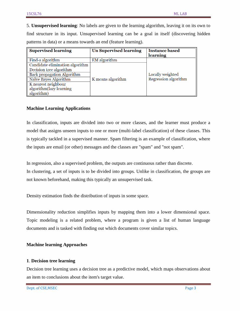
5. Unsupervised learning: No labels are given to the learning algorithm, leaving it on its own to

find structure in its input. Unsupervised learning can be a goal in itself (discovering hidden

patterns in data) or a means towards an end (feature learning).

Machine Learning Applications

In classification, inputs are divided into two or more classes, and the learner must produce a

model that assigns unseen inputs to one or more (multi-label classification) of these classes. This

is typically tackled in a supervised manner. Spam filtering is an example of classification, where

the inputs are email (or other) messages and the classes are "spam" and "not spam".

In regression, also a supervised problem, the outputs are continuous rather than discrete.

In clustering, a set of inputs is to be divided into groups. Unlike in classification, the groups are

not known beforehand, making this typically an unsupervised task.

Density estimation finds the distribution of inputs in some space.

Dimensionality reduction simplifies inputs by mapping them into a lower dimensional space.

Topic modeling is a related problem, where a program is given a list of human language

documents and is tasked with finding out which documents cover similar topics.

Machine learning Approaches

1. Decision tree learning

Decision tree learning uses a decision tree as a predictive model, which maps observations about

an item to conclusions about the item's target value.

15CSL76 ML LAB


2. Association rule learning

Association rule learning is a method for discovering interesting relations between variables in

large databases.

3. Artificial neural networks

An artificial neural network (ANN) learning algorithm, usually called "neural network" (NN), is

a learning algorithm that is vaguely inspired by biological neural networks. Computations are

structured in terms of an interconnected group of artificial neurons, processing information using

a connectionist approach to computation. Modern neural networks are non-linear statistical data

modeling tools. They are usually used to model complex relationships between inputs and

outputs, to find patterns in data, or to capture the statistical structure in an unknown joint

probability distribution between observed variables.

4. Deep learning

Falling hardware prices and the development of GPUs for personal use in the last few years have

contributed to the development of the concept of deep learning which consists of multiple hidden

layers in an artificial neural network. This approach tries to model the way the human brain

processes light and sound into vision and hearing. Some successful applications of deep learning

are computer vision and speech Recognition.

5. Inductive logic programming

Inductive logic programming (ILP) is an approach to rule learning using logic Programming as a

uniform representation for input examples, background knowledge, and hypotheses. Given an

encoding of the known background knowledge and a set of examples represented as a logical

database of facts, an ILP system will derive a hypothesized logic program that entails all positive

and no negative examples. Inductive programming is a related field that considers any kind of

programming languages for representing hypotheses (and not only logic programming), such as

functional programs.

6. Support vector machines

Support vector machines (SVMs) are a set of related supervised learning methods used for

classification and regression. Given a set of training examples, each marked as belonging to one

15CSL76 ML LAB


of two categories, an SVM training algorithm builds a model that predicts whether a new

example falls into one category or the other.

7. Clustering

Cluster analysis is the assignment of a set of observations into subsets (called clusters) so that

observations within the same cluster are similar according to some pre designated criterion or

criteria, while observations drawn from different clusters are dissimilar. Different clustering

techniques make different assumptions on the structure of the data, often defined by some

similarity metric and evaluated for example by internal compactness (similarity between

members of the same cluster) and separation between different clusters. Other methods are based

on estimated density and graph connectivity. Clustering is a method of unsupervised learning,

and a common technique for statistical data analysis.

8. Bayesian networks

A Bayesian network, belief network or directed acyclic graphical model is a probabilistic

graphical model that represents a set of random variables and their conditional independencies

via a directed acyclic graph (DAG). For example, a Bayesian network could represent the

probabilistic relationships between diseases and symptoms. Given symptoms, the network can be

used to compute the probabilities of the presence of various diseases. Efficient algorithms exist

that perform inference and learning.

9. Reinforcement learning

Reinforcement learning is concerned with how an agent ought to take actions in an environment

so as to maximize some notion of long-term reward. Reinforcement learning algorithms attempt

to find a policy that maps states of the world to the actions the agent ought to take in those states.

Reinforcement learning differs from the supervised learning problem in that correct input/output

pairs are never presented, nor sub-optimal actions explicitly corrected.

10. Similarity and metric learning

In this problem, the learning machine is given pairs of examples that are considered similar and

pairs of less similar objects. It then needs to learn a similarity function (or a distance metric

function) that can predict if new objects are similar. It is sometimes used in Recommendation

systems.

15CSL76 ML LAB


11. Genetic algorithms

A genetic algorithm (GA) is a search heuristic that mimics the process of natural selection, and

uses methods such as mutation and crossover to generate new genotype in the hope of finding

good solutions to a given problem. In machine learning, genetic algorithms found some uses in

the 1980s and 1990s. Conversely, machine learning techniques have been used to improve the

performance of genetic and evolutionary algorithms.

12. Rule-based machine learning

Rule-based machine learning is a general term for any machine learning method that identifies,

learns, or evolves "rules" to store, manipulate or apply, knowledge. The defining characteristic of

a rule- based machine learner is the identification and utilization of a set of relational rules that

collectively represent the knowledge captured by the system. This is in contrast to other machine

learners that commonly identify a singular model that can be universally applied to any instance

in order to make a prediction. Rule-based machine learning approaches include learning

classifier systems, association rule learning, and artificial immune systems.

13. Feature selection approach

Feature selection is the process of selecting an optimal subset of relevant features for use in

model construction. It is assumed the data contains some features that are either redundant or

irrelevant, and can thus be removed to reduce calculation cost without incurring much loss of

information. Common optimality criteria include accuracy, similarity and information measures.

15CSL76 ML LAB


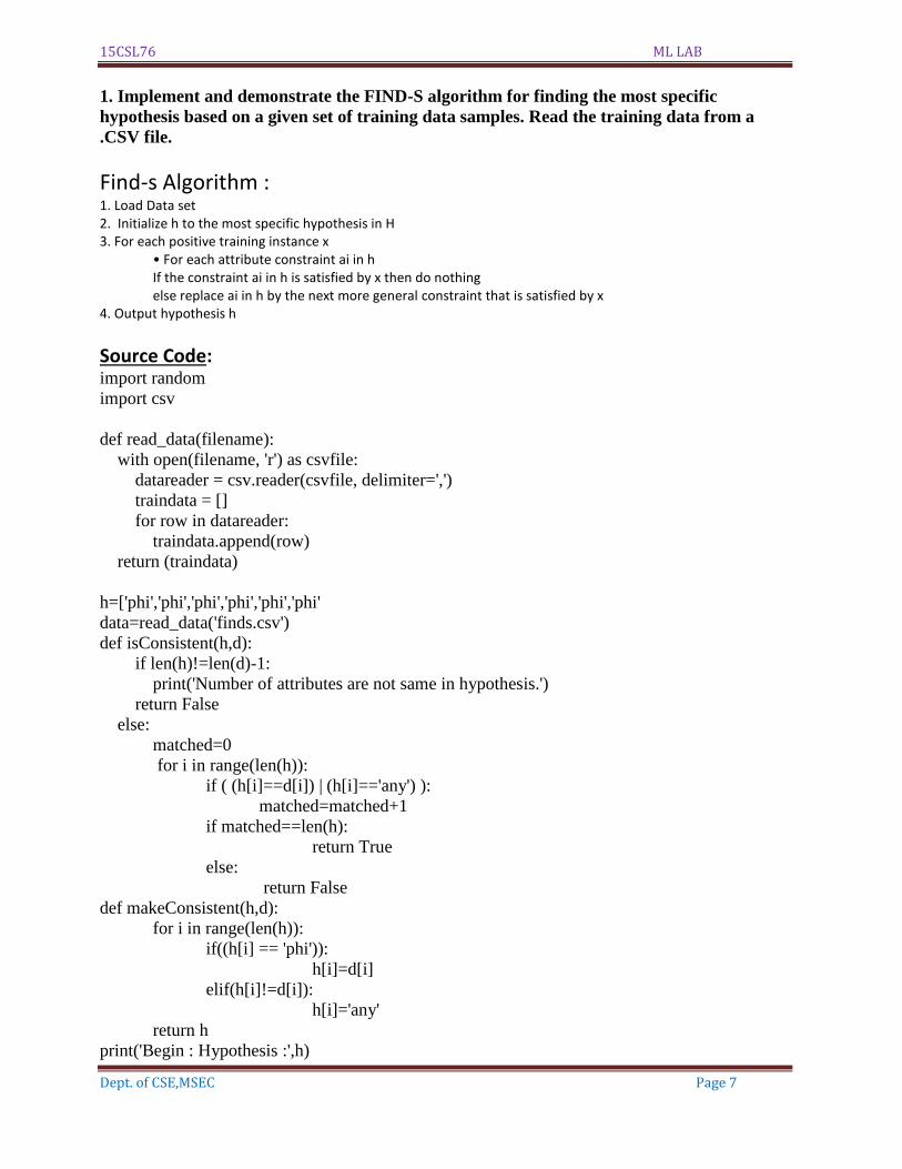
1. Implement and demonstrate the FIND-S algorithm for finding the most specific

hypothesis based on a given set of training data samples. Read the training data from a

.CSV file.

Find-s Algorithm : 1. Load Data set 2. Initialize h to the most specific hypothesis in H 3. For each positive training instance x

• For each attribute constraint ai in h If the constraint ai in h is satisfied by x then do nothing else replace ai in h by the next more general constraint that is satisfied by x

4. Output hypothesis h

Source Code: import random

import csv

def read_data(filename):

with open(filename, 'r') as csvfile:

datareader = csv.reader(csvfile, delimiter=',')

traindata = []

for row in datareader:

traindata.append(row)

return (traindata)

h=['phi','phi','phi','phi','phi','phi'

data=read_data('finds.csv')

def isConsistent(h,d):

if len(h)!=len(d)-1:

print('Number of attributes are not same in hypothesis.')

return False

else:

matched=0

for i in range(len(h)):

if ( (h[i]==d[i]) | (h[i]=='any') ):

matched=matched+1

if matched==len(h):

return True

else:

return False

def makeConsistent(h,d):

for i in range(len(h)):

if((h[i] == 'phi')):

h[i]=d[i]

elif(h[i]!=d[i]):

h[i]='any'

return h

print('Begin : Hypothesis :',h)

15CSL76 ML LAB


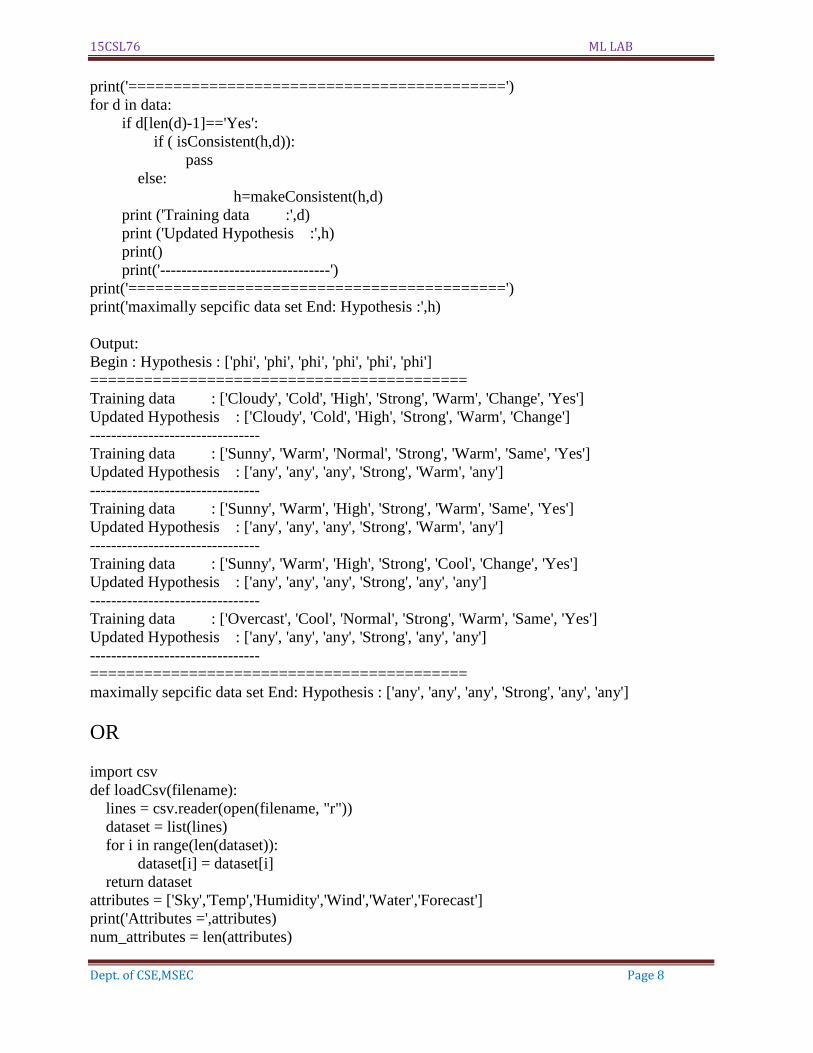
print('==========================================')

for d in data:

if d[len(d)-1]=='Yes':

if ( isConsistent(h,d)):

pass

else:

h=makeConsistent(h,d)

print ('Training data :',d)

print ('Updated Hypothesis :',h)

print()

print('--------------------------------')

print('==========================================')

print('maximally sepcific data set End: Hypothesis :',h)

Output:

Begin : Hypothesis : ['phi', 'phi', 'phi', 'phi', 'phi', 'phi']

==========================================

Training data : ['Cloudy', 'Cold', 'High', 'Strong', 'Warm', 'Change', 'Yes']

Updated Hypothesis : ['Cloudy', 'Cold', 'High', 'Strong', 'Warm', 'Change']

--------------------------------

Training data : ['Sunny', 'Warm', 'Normal', 'Strong', 'Warm', 'Same', 'Yes']

Updated Hypothesis : ['any', 'any', 'any', 'Strong', 'Warm', 'any']

--------------------------------

Training data : ['Sunny', 'Warm', 'High', 'Strong', 'Warm', 'Same', 'Yes']

Updated Hypothesis : ['any', 'any', 'any', 'Strong', 'Warm', 'any']

--------------------------------

Training data : ['Sunny', 'Warm', 'High', 'Strong', 'Cool', 'Change', 'Yes']

Updated Hypothesis : ['any', 'any', 'any', 'Strong', 'any', 'any']

--------------------------------

Training data : ['Overcast', 'Cool', 'Normal', 'Strong', 'Warm', 'Same', 'Yes']

Updated Hypothesis : ['any', 'any', 'any', 'Strong', 'any', 'any']

--------------------------------

==========================================

maximally sepcific data set End: Hypothesis : ['any', 'any', 'any', 'Strong', 'any', 'any']

OR

import csv

def loadCsv(filename):

lines = csv.reader(open(filename, "r"))

dataset = list(lines)

for i in range(len(dataset)):

dataset[i] = dataset[i]

return dataset

attributes = ['Sky','Temp','Humidity','Wind','Water','Forecast']

print('Attributes =',attributes)

num_attributes = len(attributes)

15CSL76 ML LAB


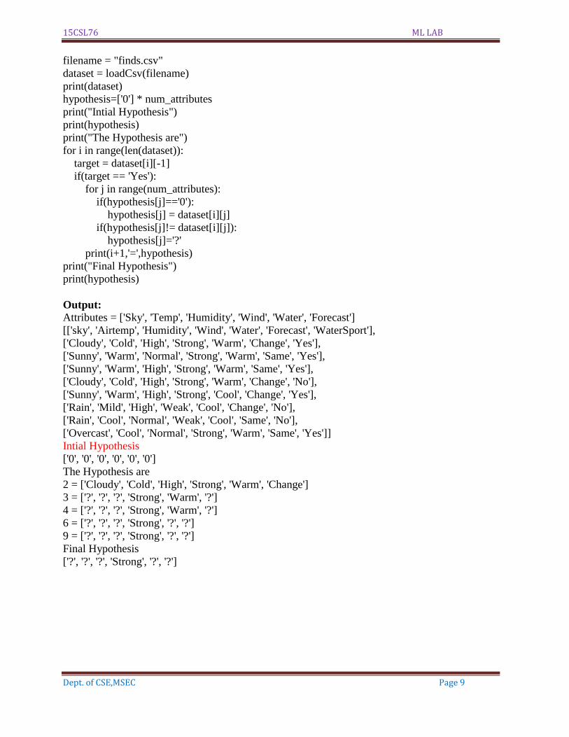
filename = "finds.csv"

dataset = loadCsv(filename)

print(dataset)

hypothesis=['0'] * num_attributes

print("Intial Hypothesis")

print(hypothesis)

print("The Hypothesis are")


target = dataset[i][-1]

if(target == 'Yes'):

for j in range(num_attributes):

if(hypothesis[j]=='0'):

hypothesis[j] = dataset[i][j]

if(hypothesis[j]!= dataset[i][j]):

hypothesis[j]='?'

print(i+1,'=',hypothesis)

print("Final Hypothesis")

print(hypothesis)

Output:

Attributes = ['Sky', 'Temp', 'Humidity', 'Wind', 'Water', 'Forecast']

[['sky', 'Airtemp', 'Humidity', 'Wind', 'Water', 'Forecast', 'WaterSport'],

['Cloudy', 'Cold', 'High', 'Strong', 'Warm', 'Change', 'Yes'],

['Sunny', 'Warm', 'Normal', 'Strong', 'Warm', 'Same', 'Yes'],

['Sunny', 'Warm', 'High', 'Strong', 'Warm', 'Same', 'Yes'],

['Cloudy', 'Cold', 'High', 'Strong', 'Warm', 'Change', 'No'],

['Sunny', 'Warm', 'High', 'Strong', 'Cool', 'Change', 'Yes'],

['Rain', 'Mild', 'High', 'Weak', 'Cool', 'Change', 'No'],

['Rain', 'Cool', 'Normal', 'Weak', 'Cool', 'Same', 'No'],

['Overcast', 'Cool', 'Normal', 'Strong', 'Warm', 'Same', 'Yes']]

Intial Hypothesis

['0', '0', '0', '0', '0', '0']

The Hypothesis are

2 = ['Cloudy', 'Cold', 'High', 'Strong', 'Warm', 'Change']

3 = ['?', '?', '?', 'Strong', 'Warm', '?']

4 = ['?', '?', '?', 'Strong', 'Warm', '?']

6 = ['?', '?', '?', 'Strong', '?', '?']

9 = ['?', '?', '?', 'Strong', '?', '?']

Final Hypothesis

['?', '?', '?', 'Strong', '?', '?']

15CSL76 ML LAB


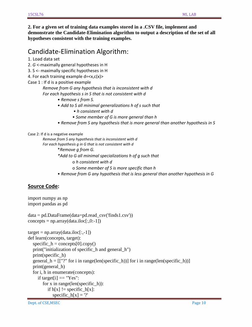
2. For a given set of training data examples stored in a .CSV file, implement and

demonstrate the Candidate-Elimination algorithm to output a description of the set of all

hypotheses consistent with the training examples.

Candidate-Elimination Algorithm: 1. Load data set 2. G <-maximally general hypotheses in H 3. S <- maximally specific hypotheses in H 4. For each training example d=<x,c(x)> Case 1 : If d is a positive example

Remove from G any hypothesis that is inconsistent with d For each hypothesis s in S that is not consistent with d

• Remove s from S. • Add to S all minimal generalizations h of s such that

• h consistent with d • Some member of G is more general than h

• Remove from S any hypothesis that is more general than another hypothesis in S Case 2: If d is a negative example

Remove from S any hypothesis that is inconsistent with d For each hypothesis g in G that is not consistent with d

*Remove g from G.

*Add to G all minimal specializations h of g such that

o h consistent with d

o Some member of S is more specific than h • Remove from G any hypothesis that is less general than another hypothesis in G

Source Code:

import numpy as np

import pandas as pd

data = pd.DataFrame(data=pd.read_csv('finds1.csv'))

concepts = np.array(data.iloc[:,0:-1])

target = np.array(data.iloc[:,-1])

def learn(concepts, target):

specific_h = concepts[0].copy()

print("initialization of specific_h and general_h")

print(specific_h)

general_h = [["?" for i in range(len(specific_h))] for i in range(len(specific_h))]

print(general_h)

for i, h in enumerate(concepts):

if target[i] == "Yes":

for x in range(len(specific_h)):

if h[x] != specific_h[x]:

specific_h[x] = '?'

15CSL76 ML LAB


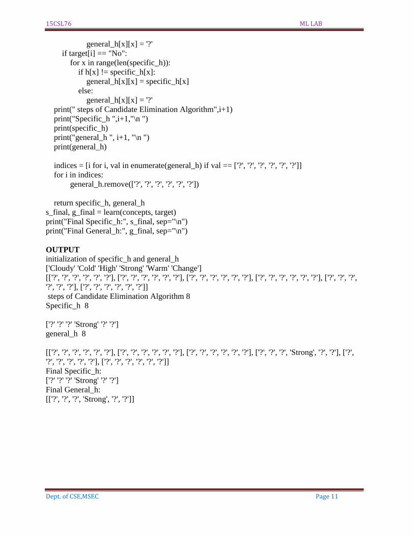
general_h[x][x] = '?'

if target[i] == "No":

for x in range(len(specific_h)):

if h[x] != specific_h[x]:

general_h[x][x] = specific_h[x]

else:

general_h[x][x] = '?'

print(" steps of Candidate Elimination Algorithm",i+1)

print("Specific_h ",i+1,"\n ")

print(specific_h)

print("general_h ", i+1, "\n ")

print(general_h)

indices = [i for i, val in enumerate(general_h) if val == ['?', '?', '?', '?', '?', '?']]

for i in indices:

general_h.remove(['?', '?', '?', '?', '?', '?'])

return specific_h, general_h

s_final, g_final = learn(concepts, target)

print("Final Specific_h:", s_final, sep="\n")

print("Final General_h:", g_final, sep="\n")

OUTPUT

initialization of specific_h and general_h

['Cloudy' 'Cold' 'High' 'Strong' 'Warm' 'Change']

[['?', '?', '?', '?', '?', '?'], ['?', '?', '?', '?', '?', '?'], ['?', '?', '?', '?', '?', '?'], ['?', '?', '?', '?', '?', '?'], ['?', '?', '?',

'?', '?', '?'], ['?', '?', '?', '?', '?', '?']]

steps of Candidate Elimination Algorithm 8

Specific_h 8

['?' '?' '?' 'Strong' '?' '?']

general_h 8

[['?', '?', '?', '?', '?', '?'], ['?', '?', '?', '?', '?', '?'], ['?', '?', '?', '?', '?', '?'], ['?', '?', '?', 'Strong', '?', '?'], ['?',

'?', '?', '?', '?', '?'], ['?', '?', '?', '?', '?', '?']]

Final Specific_h:

['?' '?' '?' 'Strong' '?' '?']

Final General_h:

[['?', '?', '?', 'Strong', '?', '?']]

15CSL76 ML LAB


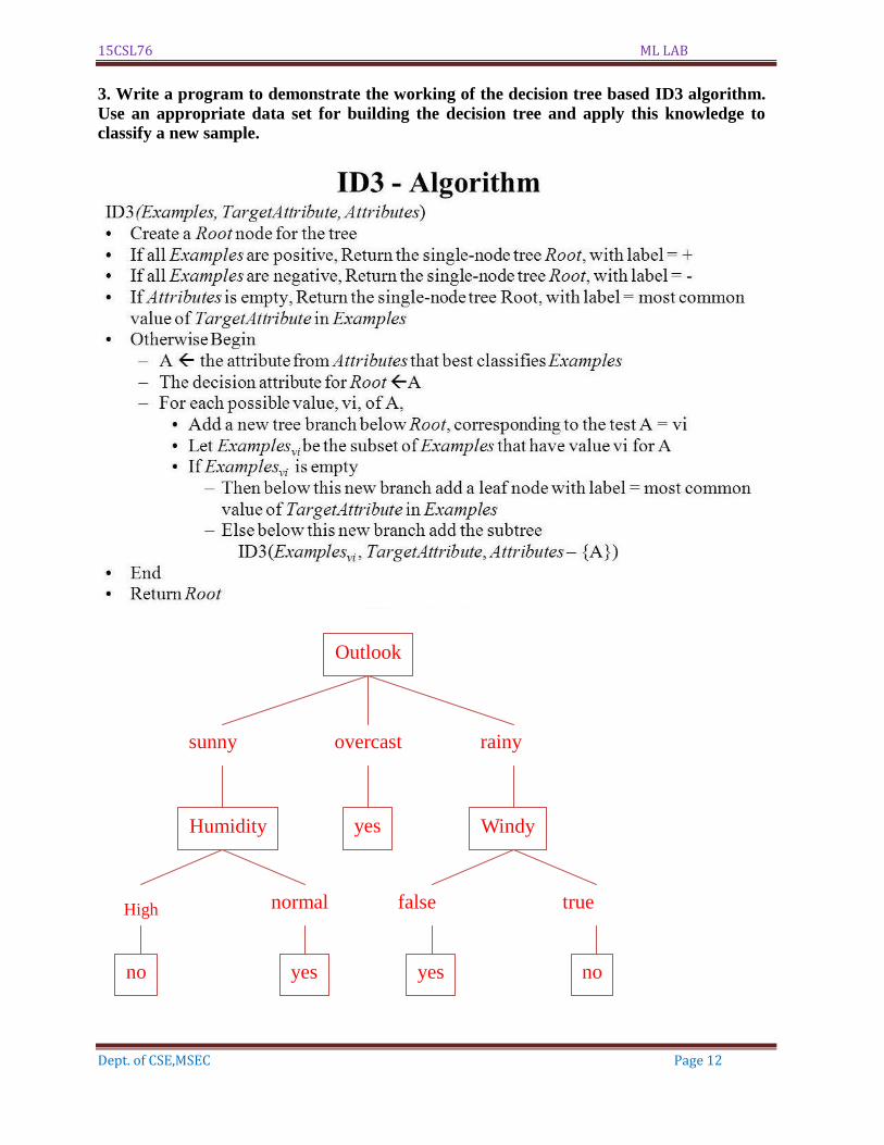
3. Write a program to demonstrate the working of the decision tree based ID3 algorithm.

Use an appropriate data set for building the decision tree and apply this knowledge to

classify a new sample.

High

Outlook

sunny overcast rainy

Humidity Windy

normal

no

false true

yes

yes yes no

15CSL76 ML LAB


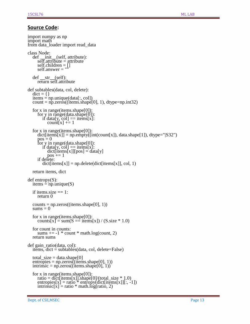
Source Code: import numpy as np import math from data_loader import read_data class Node: def __init__(self, attribute): self.attribute = attribute self.children = [] self.answer = "" def __str__(self): return self.attribute def subtables(data, col, delete): dict = {} items = np.unique(data[:, col]) count = np.zeros((items.shape[0], 1), dtype=np.int32) for x in range(items.shape[0]): for y in range(data.shape[0]): if data[y, col] == items[x]: count[x] += 1 for x in range(items.shape[0]): dict[items[x]] = np.empty((int(count[x]), data.shape[1]), dtype="|S32") pos = 0 for y in range(data.shape[0]): if data[y, col] == items[x]: dict[items[x]][pos] = data[y] pos += 1 if delete: dict[items[x]] = np.delete(dict[items[x]], col, 1) return items, dict def entropy(S): items = np.unique(S) if items.size == 1: return 0 counts = np.zeros((items.shape[0], 1)) sums = 0 for x in range(items.shape[0]): counts[x] = sum(S == items[x]) / (S.size * 1.0) for count in counts: sums += -1 * count * math.log(count, 2) return sums def gain_ratio(data, col): items, dict = subtables(data, col, delete=False) total_size = data.shape[0] entropies = np.zeros((items.shape[0], 1)) intrinsic = np.zeros((items.shape[0], 1)) for x in range(items.shape[0]): ratio = dict[items[x]].shape[0]/(total_size * 1.0) entropies[x] = ratio * entropy(dict[items[x]][:, -1]) intrinsic[x] = ratio * math.log(ratio, 2)

15CSL76 ML LAB


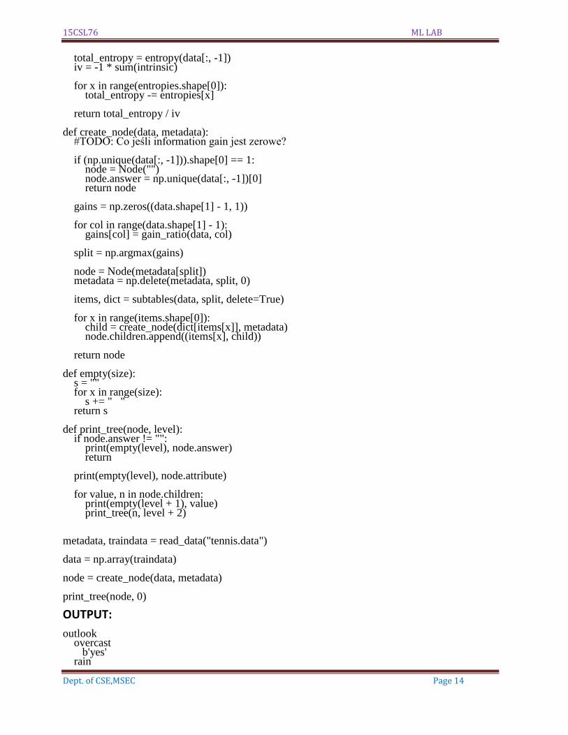
total_entropy = entropy(data[:, -1]) iv = -1 * sum(intrinsic) for x in range(entropies.shape[0]): total_entropy -= entropies[x] return total_entropy / iv def create_node(data, metadata): #TODO: Co jeśli information gain jest zerowe? if (np.unique(data[:, -1])).shape[0] == 1: node = Node("") node.answer = np.unique(data[:, -1])[0] return node gains = np.zeros((data.shape[1] - 1, 1)) for col in range(data.shape[1] - 1): gains[col] = gain_ratio(data, col) split = np.argmax(gains) node = Node(metadata[split]) metadata = np.delete(metadata, split, 0) items, dict = subtables(data, split, delete=True) for x in range(items.shape[0]): child = create_node(dict[items[x]], metadata) node.children.append((items[x], child)) return node def empty(size): s = "" for x in range(size): s += " " return s def print_tree(node, level): if node.answer != "": print(empty(level), node.answer) return print(empty(level), node.attribute) for value, n in node.children: print(empty(level + 1), value) print_tree(n, level + 2) metadata, traindata = read_data("tennis.data") data = np.array(traindata) node = create_node(data, metadata) print_tree(node, 0) OUTPUT: outlook overcast b'yes' rain

15CSL76 ML LAB


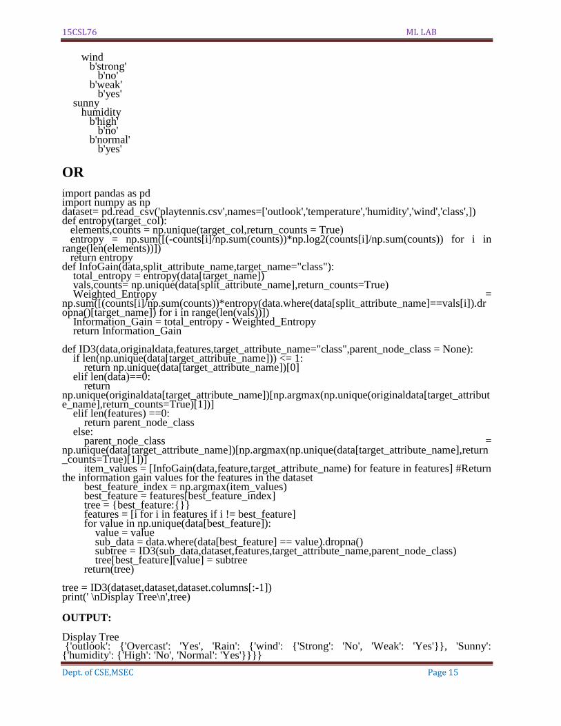
wind b'strong' b'no' b'weak' b'yes' sunny humidity b'high' b'no' b'normal' b'yes'

OR import pandas as pd import numpy as np dataset= pd.read_csv('playtennis.csv',names=['outlook','temperature','humidity','wind','class',]) def entropy(target_col): elements,counts = np.unique(target_col,return_counts = True) entropy = np.sum([(-counts[i]/np.sum(counts))*np.log2(counts[i]/np.sum(counts)) for i in range(len(elements))]) return entropy def InfoGain(data,split_attribute_name,target_name="class"): total_entropy = entropy(data[target_name]) vals,counts= np.unique(data[split_attribute_name],return_counts=True) Weighted_Entropy = np.sum([(counts[i]/np.sum(counts))*entropy(data.where(data[split_attribute_name]==vals[i]).dropna()[target_name]) for i in range(len(vals))]) Information_Gain = total_entropy - Weighted_Entropy return Information_Gain def ID3(data,originaldata,features,target_attribute_name="class",parent_node_class = None): if len(np.unique(data[target_attribute_name])) <= 1: return np.unique(data[target_attribute_name])[0] elif len(data)==0: return np.unique(originaldata[target_attribute_name])[np.argmax(np.unique(originaldata[target_attribute_name],return_counts=True)[1])] elif len(features) ==0: return parent_node_class else: parent_node_class = np.unique(data[target_attribute_name])[np.argmax(np.unique(data[target_attribute_name],return_counts=True)[1])] item_values = [InfoGain(data,feature,target_attribute_name) for feature in features] #Return the information gain values for the features in the dataset best_feature_index = np.argmax(item_values) best_feature = features[best_feature_index] tree = {best_feature:{}} features = [i for i in features if i != best_feature] for value in np.unique(data[best_feature]): value = value sub_data = data.where(data[best_feature] == value).dropna() subtree = ID3(sub_data,dataset,features,target_attribute_name,parent_node_class) tree[best_feature][value] = subtree return(tree) tree = ID3(dataset,dataset,dataset.columns[:-1]) print(' \nDisplay Tree\n',tree) OUTPUT: Display Tree {'outlook': {'Overcast': 'Yes', 'Rain': {'wind': {'Strong': 'No', 'Weak': 'Yes'}}, 'Sunny': {'humidity': {'High': 'No', 'Normal': 'Yes'}}}}

15CSL76 ML LAB


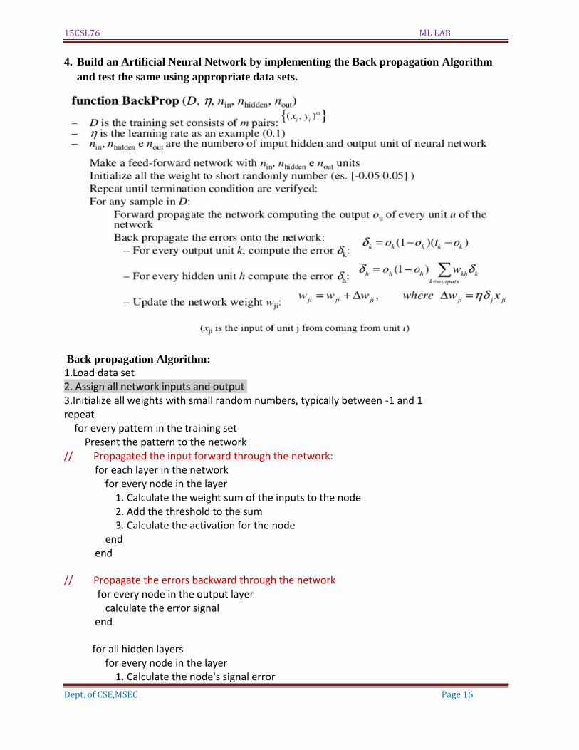
4. Build an Artificial Neural Network by implementing the Back propagation Algorithm

and test the same using appropriate data sets.

Back propagation Algorithm:

1.Load data set 2. Assign all network inputs and output 3.Initialize all weights with small random numbers, typically between -1 and 1 repeat for every pattern in the training set Present the pattern to the network // Propagated the input forward through the network: for each layer in the network for every node in the layer 1. Calculate the weight sum of the inputs to the node 2. Add the threshold to the sum 3. Calculate the activation for the node end end

// Propagate the errors backward through the network for every node in the output layer calculate the error signal end

for all hidden layers for every node in the layer 1. Calculate the node's signal error

15CSL76 ML LAB


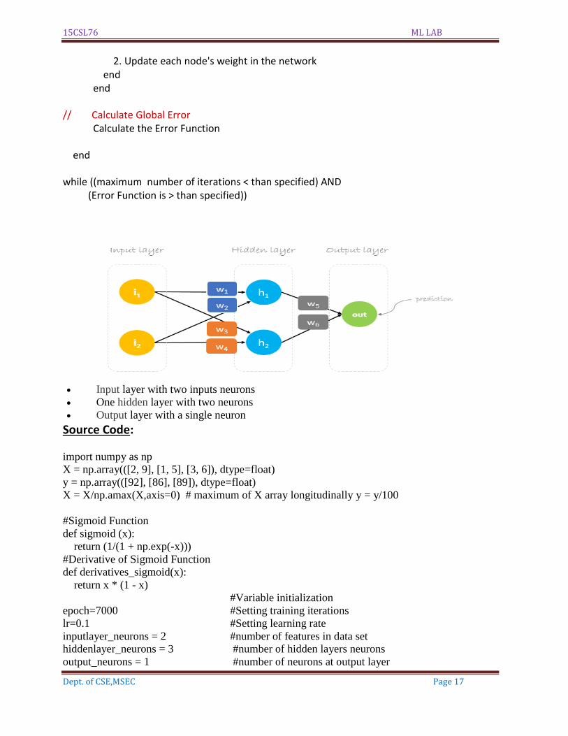
2. Update each node's weight in the network end end

// Calculate Global Error Calculate the Error Function

end

while ((maximum number of iterations < than specified) AND (Error Function is > than specified))

Input layer with two inputs neurons

One hidden layer with two neurons

Output layer with a single neuron

Source Code:

import numpy as np

X = np.array(([2, 9], [1, 5], [3, 6]), dtype=float)

y = np.array(([92], [86], [89]), dtype=float)

X = X/np.amax(X,axis=0) # maximum of X array longitudinally y = y/100

#Sigmoid Function

def sigmoid (x):

return (1/(1 + np.exp(-x)))

#Derivative of Sigmoid Function

def derivatives_sigmoid(x):

return x * (1 - x)

#Variable initialization

epoch=7000 #Setting training iterations

lr=0.1 #Setting learning rate

inputlayer_neurons = 2 #number of features in data set

hiddenlayer_neurons = 3 #number of hidden layers neurons

output_neurons = 1 #number of neurons at output layer

15CSL76 ML LAB


#weight and bias initialization

wh=np.random.uniform(size=(inputlayer_neurons,hiddenlayer_neurons))

bh=np.random.uniform(size=(1,hiddenlayer_neurons))

wout=np.random.uniform(size=(hiddenlayer_neurons,output_neurons))

bout=np.random.uniform(size=(1,output_neurons))

# draws a random range of numbers uniformly of dim x*y

#Forward Propagation

for i in range(epoch):

hinp1=np.dot(X,wh)

hinp=hinp1 + bh

hlayer_act = sigmoid(hinp)

outinp1=np.dot(hlayer_act,wout)

outinp= outinp1+ bout

output = sigmoid(outinp)

#Backpropagation

EO = y-output

outgrad = derivatives_sigmoid(output)

d_output = EO* outgrad

EH = d_output.dot(wout.T)

hiddengrad = derivatives_sigmoid(hlayer_act)

#how much hidden layer wts contributed to error

d_hiddenlayer = EH * hiddengrad

wout += hlayer_act.T.dot(d_output) *lr

# dotproduct of nextlayererror and currentlayerop

bout += np.sum(d_output, axis=0,keepdims=True) *lr

wh += X.T.dot(d_hiddenlayer) *lr

#bh += np.sum(d_hiddenlayer, axis=0,keepdims=True) *lr

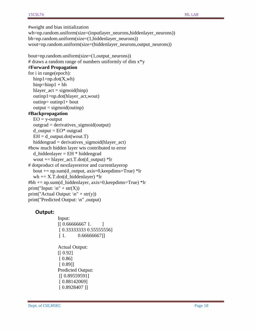
print("Input: \n" + str(X))

print("Actual Output: \n" + str(y))

print("Predicted Output: \n" ,output)

Output: Input:

[[ 0.66666667 1. ]

[ 0.33333333 0.55555556]

[ 1. 0.66666667]]

Actual Output:

[[ 0.92]

[ 0.86]

[ 0.89]]

Predicted Output:

[[ 0.89559591]

[ 0.88142069]

[ 0.8928407 ]]

15CSL76 ML LAB


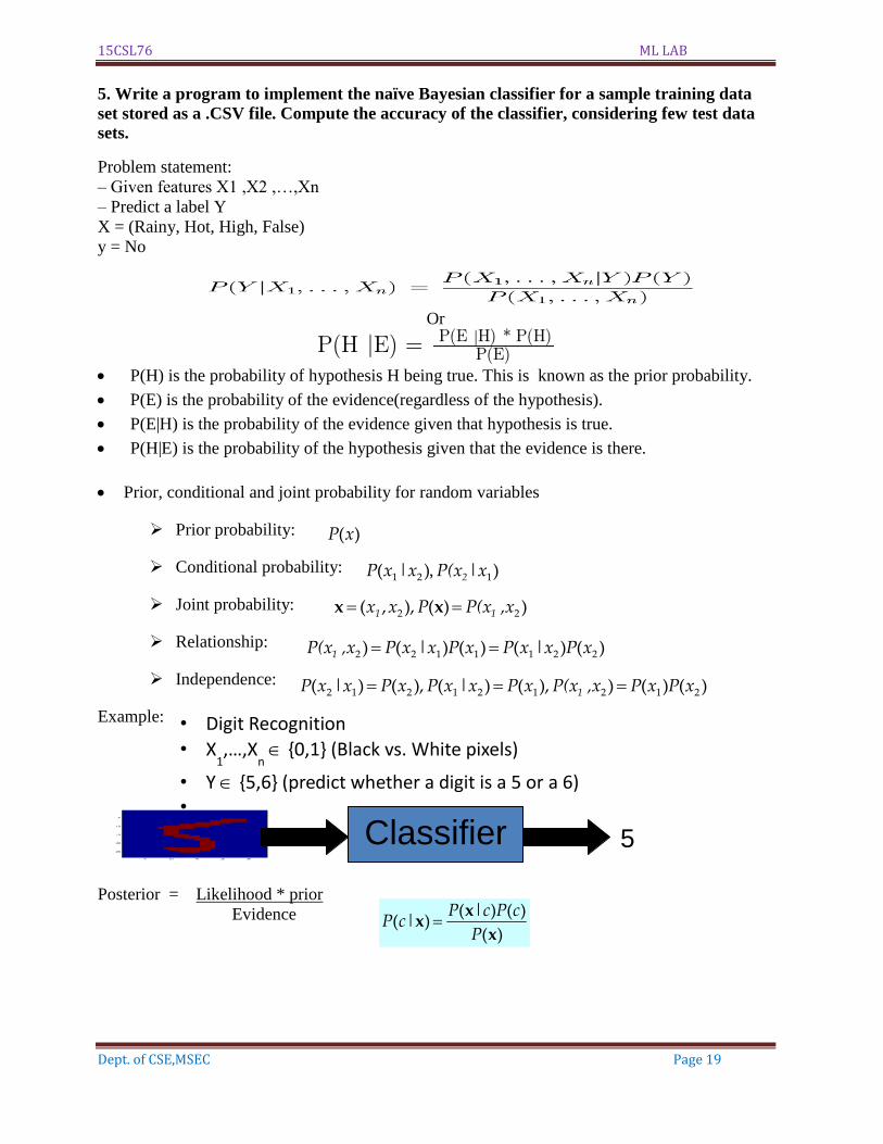
5. Write a program to implement the naïve Bayesian classifier for a sample training data

set stored as a .CSV file. Compute the accuracy of the classifier, considering few test data

sets.

Problem statement:

– Given features X1 ,X2 ,…,Xn

– Predict a label Y

X = (Rainy, Hot, High, False)

y = No

Or

P(H) is the probability of hypothesis H being true. This is known as the prior probability.

P(E) is the probability of the evidence(regardless of the hypothesis).

P(E|H) is the probability of the evidence given that hypothesis is true.

P(H|E) is the probability of the hypothesis given that the evidence is there.

Prior, conditional and joint probability for random variables

Prior probability:

Conditional probability:

Joint probability:

Relationship:

Independence:

Example:

Posterior = Likelihood * prior

Evidence

Classifier 5

• Digit Recognition

• X1,…,X

n {0,1} (Black vs. White pixels)

• Y {5,6} (predict whether a digit is a 5 or a 6) •

)(xP

)|)( 121 xP(xx|xP 2 ,

))(),,( 22 ,xP(xPxx 11 xx

)()|()()|() 2211122 xPxxPxPxxP,xP(x1

)()()),()|(),()|( 212121212 xPxP,xP(xxPxxPxPxxP 1

)(

)()()(

x

xx

P

cPc|P|cP

15CSL76 ML LAB


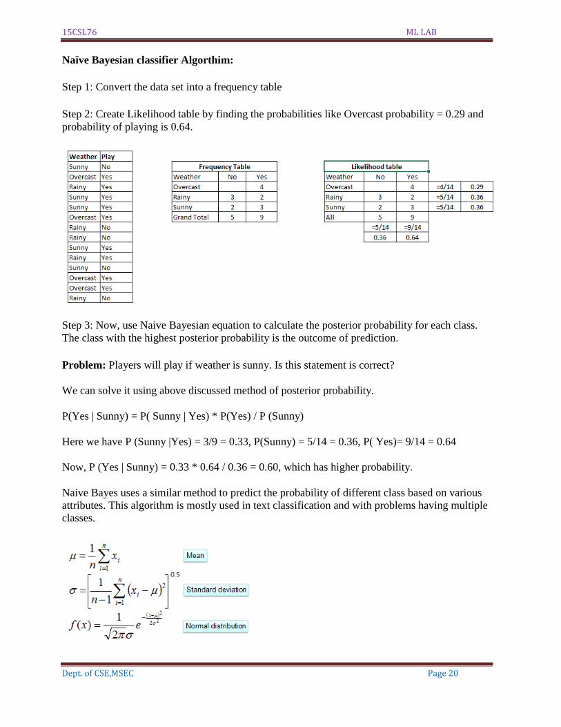
Naïve Bayesian classifier Algorthim:

Step 1: Convert the data set into a frequency table

Step 2: Create Likelihood table by finding the probabilities like Overcast probability = 0.29 and

probability of playing is 0.64.

Step 3: Now, use Naive Bayesian equation to calculate the posterior probability for each class.

The class with the highest posterior probability is the outcome of prediction.

Problem: Players will play if weather is sunny. Is this statement is correct?

We can solve it using above discussed method of posterior probability.

P(Yes | Sunny) = P( Sunny | Yes) * P(Yes) / P (Sunny)

Here we have P (Sunny |Yes) = 3/9 = 0.33, P(Sunny) = 5/14 = 0.36, P( Yes)= 9/14 = 0.64

Now, P (Yes | Sunny) = 0.33 * 0.64 / 0.36 = 0.60, which has higher probability.

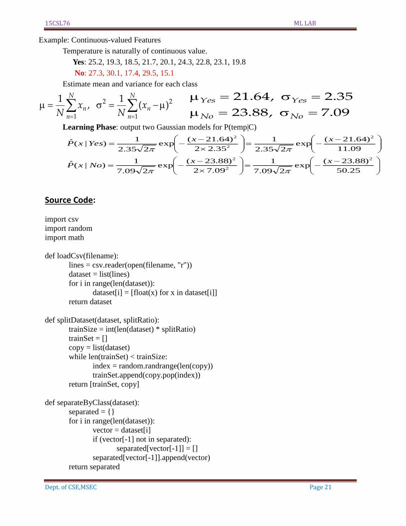
Naive Bayes uses a similar method to predict the probability of different class based on various

attributes. This algorithm is mostly used in text classification and with problems having multiple

classes.

https://www.analyticsvidhya.com/wp-content/uploads/2015/08/Bayes_41.png

https://www.analyticsvidhya.com/wp-content/uploads/2015/08/Bayes_41.png

15CSL76 ML LAB


Source Code:

import csv

import random

import math

def loadCsv(filename):

lines = csv.reader(open(filename, "r"))

dataset = list(lines)


dataset[i] = [float(x) for x in dataset[i]]

return dataset

def splitDataset(dataset, splitRatio):

trainSize = int(len(dataset) * splitRatio)

trainSet = []

copy = list(dataset)

while len(trainSet) < trainSize:

index = random.randrange(len(copy))

trainSet.append(copy.pop(index))

return [trainSet, copy]

def separateByClass(dataset):

separated = {}


vector = dataset[i]

if (vector[-1] not in separated):

separated[vector[-1]] = []

separated[vector[-1]].append(vector)

return separated

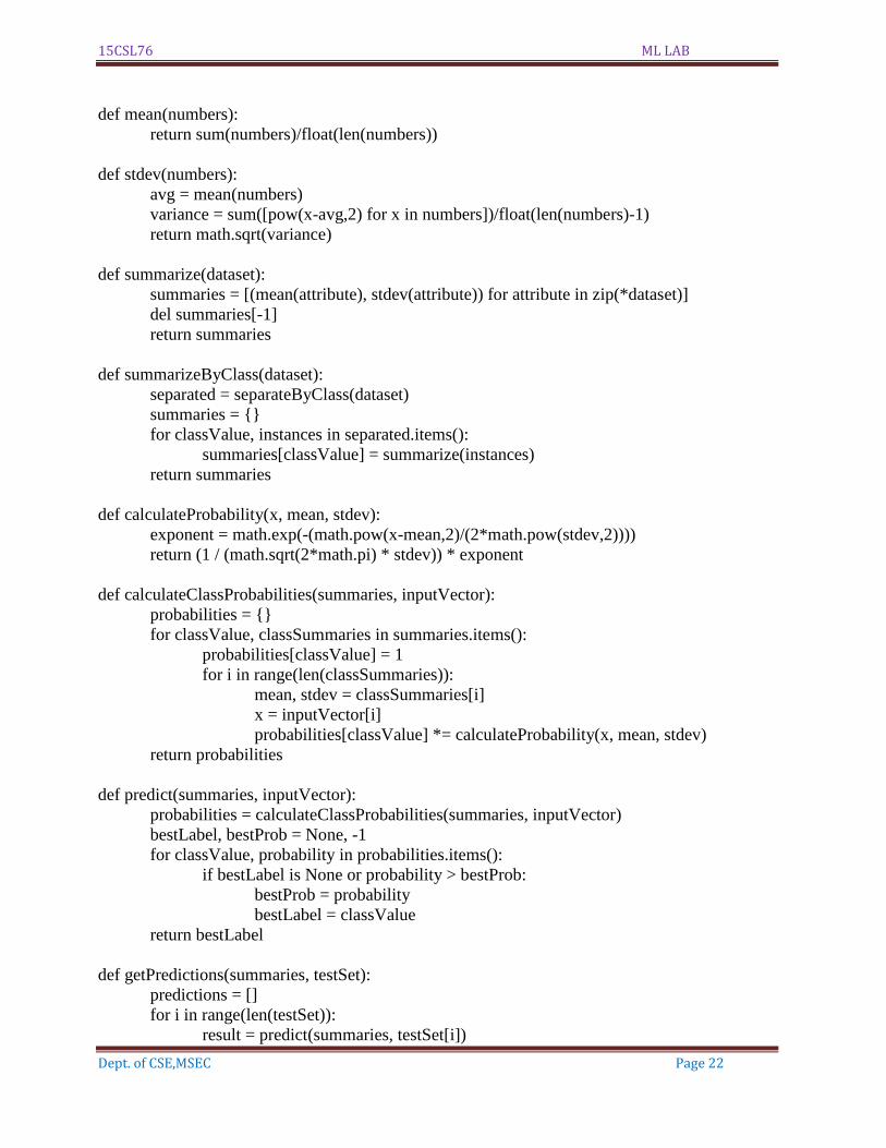
Example: Continuous-valued Features

Temperature is naturally of continuous value.

Yes: 25.2, 19.3, 18.5, 21.7, 20.1, 24.3, 22.8, 23.1, 19.8

No: 27.3, 30.1, 17.4, 29.5, 15.1

Estimate mean and variance for each class

N

nn

N

nn x

Nx

N 1

22

1

)(1

,1

09.7 ,88.23

35.2 ,64.21

NoNo

YesYes

Learning Phase: output two Gaussian models for P(temp|C)

25.50

)88.23(exp

209.7

1

09.72

)88.23(exp

209.7

1)|(ˆ

09.11

)64.21(exp

235.2

1

35.22

)64.21(exp

235.2

1)|(ˆ

2

2

2

2

2

2

xxNoxP

xxYesxP

15CSL76 ML LAB


def mean(numbers):

return sum(numbers)/float(len(numbers))

def stdev(numbers):

avg = mean(numbers)

variance = sum([pow(x-avg,2) for x in numbers])/float(len(numbers)-1)

return math.sqrt(variance)

def summarize(dataset):

summaries = [(mean(attribute), stdev(attribute)) for attribute in zip(*dataset)]

del summaries[-1]

return summaries

def summarizeByClass(dataset):

separated = separateByClass(dataset)

summaries = {}

for classValue, instances in separated.items():

summaries[classValue] = summarize(instances)

return summaries

def calculateProbability(x, mean, stdev):

exponent = math.exp(-(math.pow(x-mean,2)/(2*math.pow(stdev,2))))

return (1 / (math.sqrt(2*math.pi) * stdev)) * exponent

def calculateClassProbabilities(summaries, inputVector):

probabilities = {}

for classValue, classSummaries in summaries.items():

probabilities[classValue] = 1

for i in range(len(classSummaries)):

mean, stdev = classSummaries[i]

x = inputVector[i]

probabilities[classValue] *= calculateProbability(x, mean, stdev)

return probabilities

def predict(summaries, inputVector):

probabilities = calculateClassProbabilities(summaries, inputVector)

bestLabel, bestProb = None, -1

for classValue, probability in probabilities.items():

if bestLabel is None or probability > bestProb:

bestProb = probability

bestLabel = classValue

return bestLabel

def getPredictions(summaries, testSet):

predictions = []

for i in range(len(testSet)):

result = predict(summaries, testSet[i])

15CSL76 ML LAB


predictions.append(result)

return predictions

def getAccuracy(testSet, predictions):

correct = 0

for i in range(len(testSet)):

if testSet[i][-1] == predictions[i]:

correct += 1

return (correct/float(len(testSet))) * 100.0

def main():

filename = 'data.csv'

splitRatio = 0.67

dataset = loadCsv(filename)

trainingSet, testSet = splitDataset(dataset, splitRatio)

print('Split {0} rows into train={1} and test={2} rows'.format(len(dataset),

len(trainingSet), len(testSet)))

# prepare model

summaries = summarizeByClass(trainingSet)

# test model

predictions = getPredictions(summaries, testSet)

accuracy = getAccuracy(testSet, predictions)

print('Accuracy: {0}%'.format(accuracy))

main()

OUTPUT :

Split 306 rows into train=205 and test=101 rows

Accuracy: 72.27722772277228%

15CSL76 ML LAB


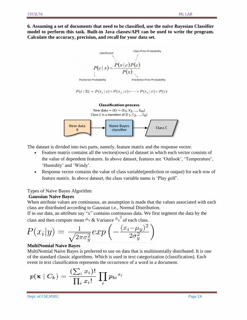
6. Assuming a set of documents that need to be classified, use the naïve Bayesian Classifier

model to perform this task. Built-in Java classes/API can be used to write the program.

Calculate the accuracy, precision, and recall for your data set.

The dataset is divided into two parts, namely, feature matrix and the response vector.

Feature matrix contains all the vectors(rows) of dataset in which each vector consists of

the value of dependent features. In above dataset, features are ‘Outlook’, ‘Temperature’,

‘Humidity’ and ‘Windy’.

Response vector contains the value of class variable(prediction or output) for each row of

feature matrix. In above dataset, the class variable name is ‘Play golf’.

Types of Naive Bayes Algorithm

Gaussian Naive Bayes

When attribute values are continuous, an assumption is made that the values associated with each

class are distributed according to Gaussian i.e., Normal Distribution.

If in our data, an attribute say “x” contains continuous data. We first segment the data by the

class and then compute mean & Variance of each class.

MultiNomial Naive Bayes

MultiNomial Naive Bayes is preferred to use on data that is multinomially distributed. It is one

of the standard classic algorithms. Which is used in text categorization (classification). Each

event in text classification represents the occurrence of a word in a document.

15CSL76 ML LAB


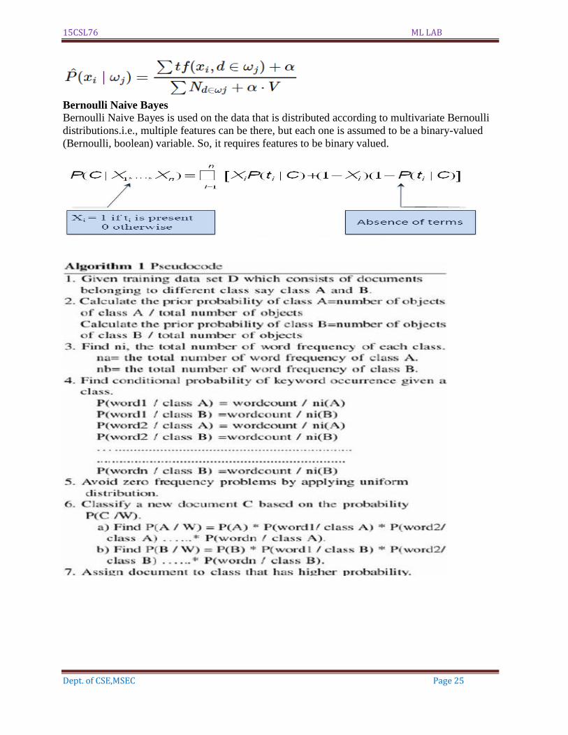
Bernoulli Naive Bayes

Bernoulli Naive Bayes is used on the data that is distributed according to multivariate Bernoulli

distributions.i.e., multiple features can be there, but each one is assumed to be a binary-valued

(Bernoulli, boolean) variable. So, it requires features to be binary valued.

15CSL76 ML LAB


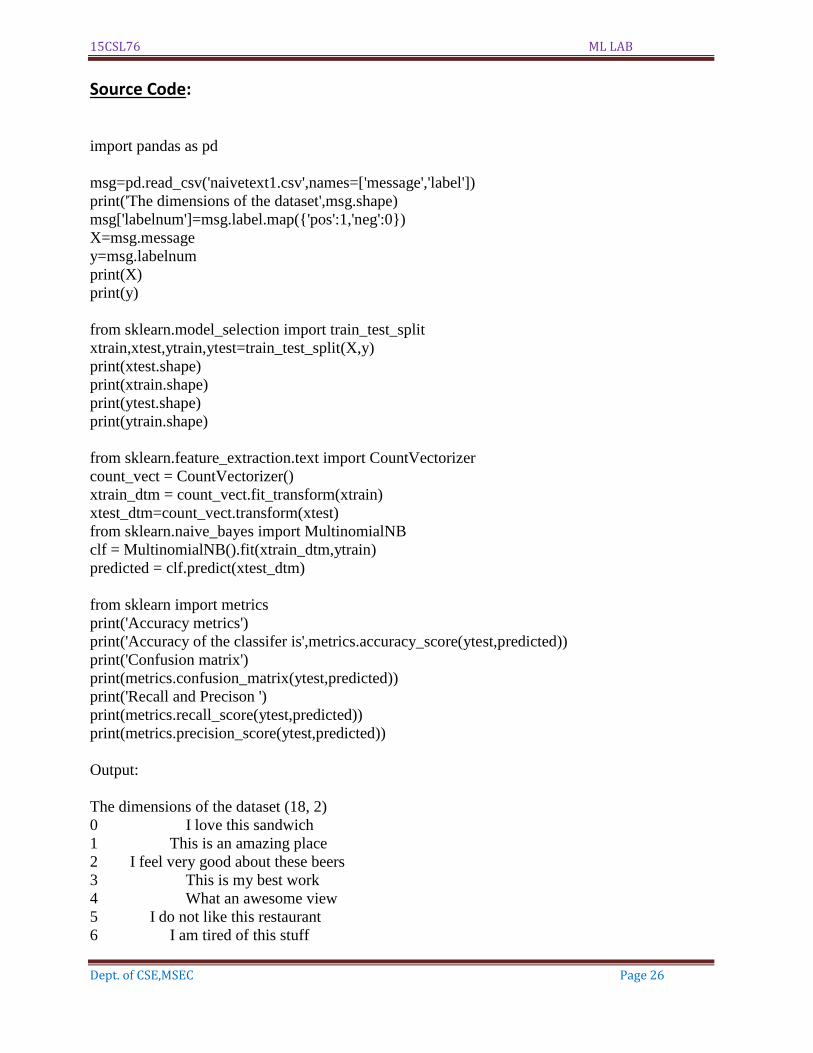
Source Code:

import pandas as pd

msg=pd.read_csv('naivetext1.csv',names=['message','label'])

print('The dimensions of the dataset',msg.shape)

msg['labelnum']=msg.label.map({'pos':1,'neg':0})

X=msg.message

y=msg.labelnum

print(X)

print(y)

from sklearn.model_selection import train_test_split

xtrain,xtest,ytrain,ytest=train_test_split(X,y)

print(xtest.shape)

print(xtrain.shape)

print(ytest.shape)

print(ytrain.shape)

from sklearn.feature_extraction.text import CountVectorizer

count_vect = CountVectorizer()

xtrain_dtm = count_vect.fit_transform(xtrain)

xtest_dtm=count_vect.transform(xtest)

from sklearn.naive_bayes import MultinomialNB

clf = MultinomialNB().fit(xtrain_dtm,ytrain)

predicted = clf.predict(xtest_dtm)

from sklearn import metrics

print('Accuracy metrics')

print('Accuracy of the classifer is',metrics.accuracy_score(ytest,predicted))

print('Confusion matrix')

print(metrics.confusion_matrix(ytest,predicted))

print('Recall and Precison ')

print(metrics.recall_score(ytest,predicted))

print(metrics.precision_score(ytest,predicted))

Output:

The dimensions of the dataset (18, 2)

0 I love this sandwich

1 This is an amazing place

2 I feel very good about these beers

3 This is my best work

4 What an awesome view

5 I do not like this restaurant

6 I am tired of this stuff

15CSL76 ML LAB


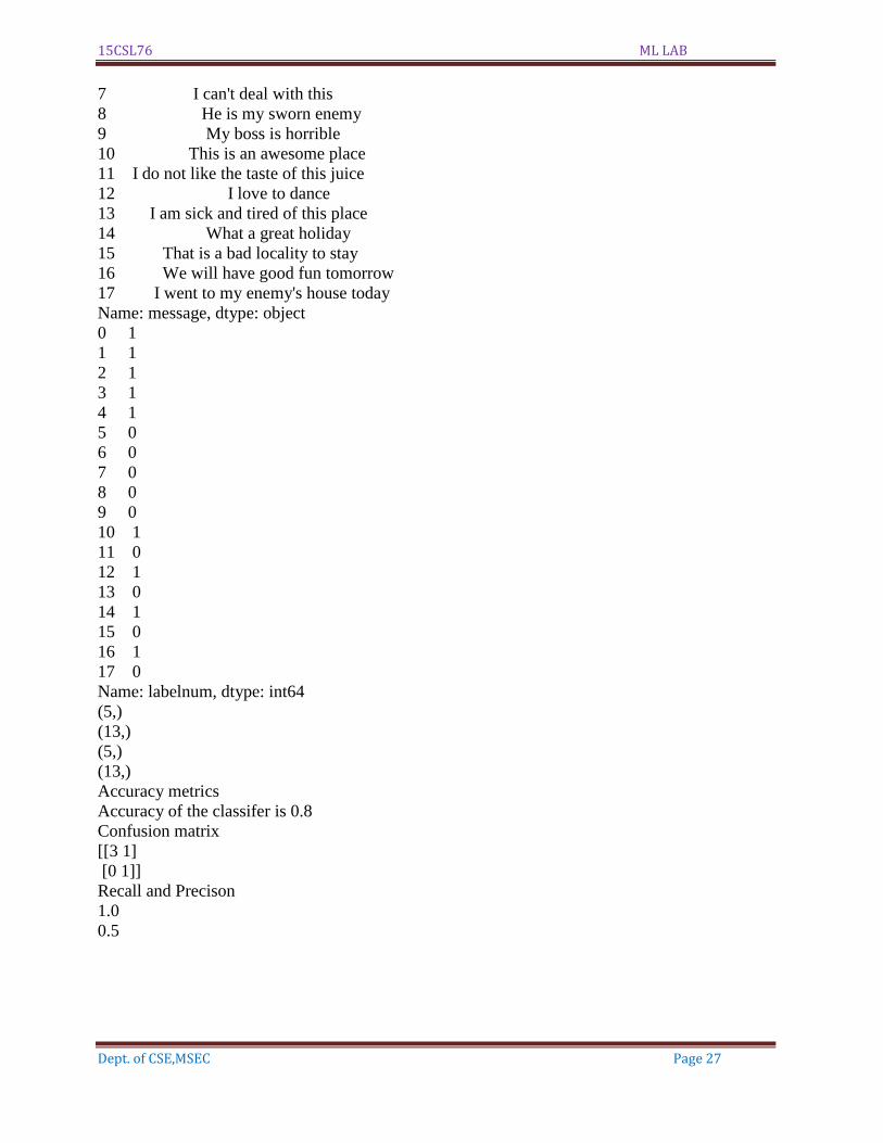
7 I can't deal with this

8 He is my sworn enemy

9 My boss is horrible

10 This is an awesome place

11 I do not like the taste of this juice

12 I love to dance

13 I am sick and tired of this place

14 What a great holiday

15 That is a bad locality to stay

16 We will have good fun tomorrow

17 I went to my enemy's house today

Name: message, dtype: object

0 1

1 1

2 1

3 1

4 1

5 0

6 0

7 0

8 0

9 0

10 1

11 0

12 1

13 0

14 1

15 0

16 1

17 0

Name: labelnum, dtype: int64

(5,)

(13,)

(5,)

(13,)

Accuracy metrics

Accuracy of the classifer is 0.8

Confusion matrix

[[3 1]

[0 1]]

Recall and Precison

1.0

0.5

15CSL76 ML LAB


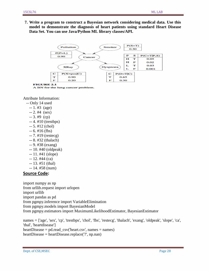
7. Write a program to construct a Bayesian network considering medical data. Use this

model to demonstrate the diagnosis of heart patients using standard Heart Disease

Data Set. You can use Java/Python ML library classes/API.

Attribute Information: -- Only 14 used -- 1. #3 (age) -- 2. #4 (sex) -- 3. #9 (cp)

-- 4. #10 (trestbps) -- 5. #12 (chol) -- 6. #16 (fbs) -- 7. #19 (restecg) -- 8. #32 (thalach) -- 9. #38 (exang) -- 10. #40 (oldpeak) -- 11. #41 (slope) -- 12. #44 (ca) -- 13. #51 (thal) -- 14. #58 (num)

Source Code: import numpy as np

from urllib.request import urlopen

import urllib

import pandas as pd

from pgmpy.inference import VariableElimination

from pgmpy.models import BayesianModel from pgmpy.estimators import MaximumLikelihoodEstimator, BayesianEstimator

names = ['age', 'sex', 'cp', 'trestbps', 'chol', 'fbs', 'restecg', 'thalach', 'exang', 'oldpeak', 'slope', 'ca', 'thal', 'heartdisease']

heartDisease = pd.read_csv('heart.csv', names = names) heartDisease = heartDisease.replace('?', np.nan)

15CSL76 ML LAB


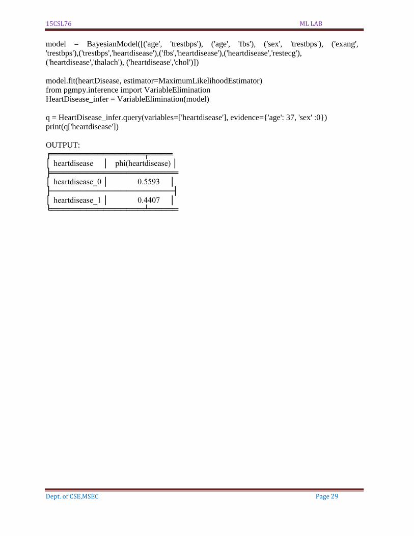
model = BayesianModel([('age', 'trestbps'), ('age', 'fbs'), ('sex', 'trestbps'), ('exang', 'trestbps'),('trestbps','heartdisease'),('fbs','heartdisease'),('heartdisease','restecg'), ('heartdisease','thalach'), ('heartdisease','chol')])

model.fit(heartDisease, estimator=MaximumLikelihoodEstimator) from pgmpy.inference import VariableElimination

HeartDisease_infer = VariableElimination(model)

q = HeartDisease_infer.query(variables=['heartdisease'], evidence={'age': 37, 'sex' :0}) print(q['heartdisease']) OUTPUT: ╒════════════════╤════ │ heartdisease │ phi(heartdisease) │ ╞══════════════════════ │ heartdisease_0 │ 0.5593 │ ├─────────────────────┤

│ heartdisease_1 │ 0.4407 │ ╘════════════════╧═════

15CSL76 ML LAB


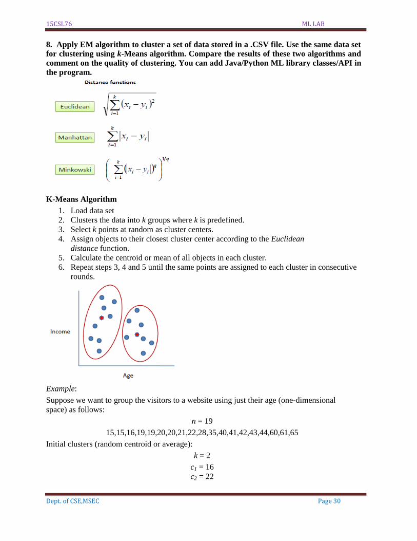
8. Apply EM algorithm to cluster a set of data stored in a .CSV file. Use the same data set

for clustering using k-Means algorithm. Compare the results of these two algorithms and

comment on the quality of clustering. You can add Java/Python ML library classes/API in

the program.

K-Means Algorithm

1. Load data set

2. Clusters the data into k groups where k is predefined.

3. Select k points at random as cluster centers.

4. Assign objects to their closest cluster center according to the Euclidean

distance function.

5. Calculate the centroid or mean of all objects in each cluster.

6. Repeat steps 3, 4 and 5 until the same points are assigned to each cluster in consecutive

rounds.

Example:

Suppose we want to group the visitors to a website using just their age (one-dimensional

space) as follows:

n = 19

15,15,16,19,19,20,20,21,22,28,35,40,41,42,43,44,60,61,65

Initial clusters (random centroid or average):

k = 2

c1 = 16

c2 = 22

15CSL76 ML LAB


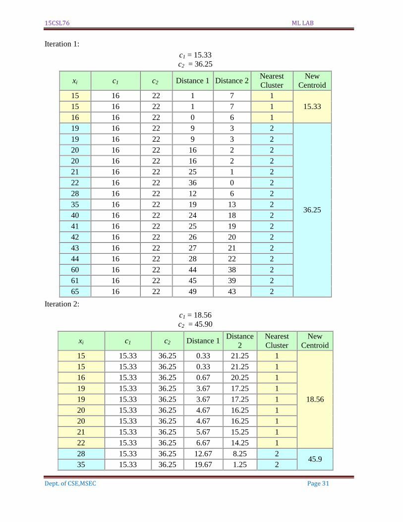
Iteration 1:

c1 = 15.33

c2 = 36.25

xi c1 c2 Distance 1 Distance 2 Nearest

Cluster

New

Centroid

15 16 22 1 7 1

15.33 15 16 22 1 7 1

16 16 22 0 6 1

19 16 22 9 3 2

36.25

19 16 22 9 3 2

20 16 22 16 2 2

20 16 22 16 2 2

21 16 22 25 1 2

22 16 22 36 0 2

28 16 22 12 6 2

35 16 22 19 13 2

40 16 22 24 18 2

41 16 22 25 19 2

42 16 22 26 20 2

43 16 22 27 21 2

44 16 22 28 22 2

60 16 22 44 38 2

61 16 22 45 39 2

65 16 22 49 43 2

Iteration 2:

c1 = 18.56

c2 = 45.90

xi c1 c2 Distance 1 Distance

2

Nearest

Cluster

New

Centroid

15 15.33 36.25 0.33 21.25 1

18.56

15 15.33 36.25 0.33 21.25 1

16 15.33 36.25 0.67 20.25 1

19 15.33 36.25 3.67 17.25 1

19 15.33 36.25 3.67 17.25 1

20 15.33 36.25 4.67 16.25 1

20 15.33 36.25 4.67 16.25 1

21 15.33 36.25 5.67 15.25 1

22 15.33 36.25 6.67 14.25 1

28 15.33 36.25 12.67 8.25 2 45.9

35 15.33 36.25 19.67 1.25 2

15CSL76 ML LAB


40 15.33 36.25 24.67 3.75 2

41 15.33 36.25 25.67 4.75 2

42 15.33 36.25 26.67 5.75 2

43 15.33 36.25 27.67 6.75 2

44 15.33 36.25 28.67 7.75 2

60 15.33 36.25 44.67 23.75 2

61 15.33 36.25 45.67 24.75 2

65 15.33 36.25 49.67 28.75 2

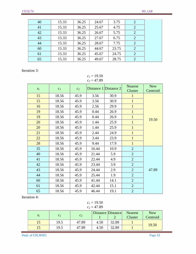
Iteration 3:

c1 = 19.50

c2 = 47.89

xi c1 c2 Distance 1 Distance 2 Nearest

Cluster

New

Centroid

15 18.56 45.9 3.56 30.9 1

19.50

15 18.56 45.9 3.56 30.9 1

16 18.56 45.9 2.56 29.9 1

19 18.56 45.9 0.44 26.9 1

19 18.56 45.9 0.44 26.9 1

20 18.56 45.9 1.44 25.9 1

20 18.56 45.9 1.44 25.9 1

21 18.56 45.9 2.44 24.9 1

22 18.56 45.9 3.44 23.9 1

28 18.56 45.9 9.44 17.9 1

35 18.56 45.9 16.44 10.9 2

47.89

40 18.56 45.9 21.44 5.9 2

41 18.56 45.9 22.44 4.9 2

42 18.56 45.9 23.44 3.9 2

43 18.56 45.9 24.44 2.9 2

44 18.56 45.9 25.44 1.9 2

60 18.56 45.9 41.44 14.1 2

61 18.56 45.9 42.44 15.1 2

65 18.56 45.9 46.44 19.1 2

Iteration 4:

c1 = 19.50

c2 = 47.89

xi c1 c2 Distance

1

Distance

2

Nearest

Cluster

New

Centroid

15 19.5 47.89 4.50 32.89 1 19.50

15 19.5 47.89 4.50 32.89 1

15CSL76 ML LAB


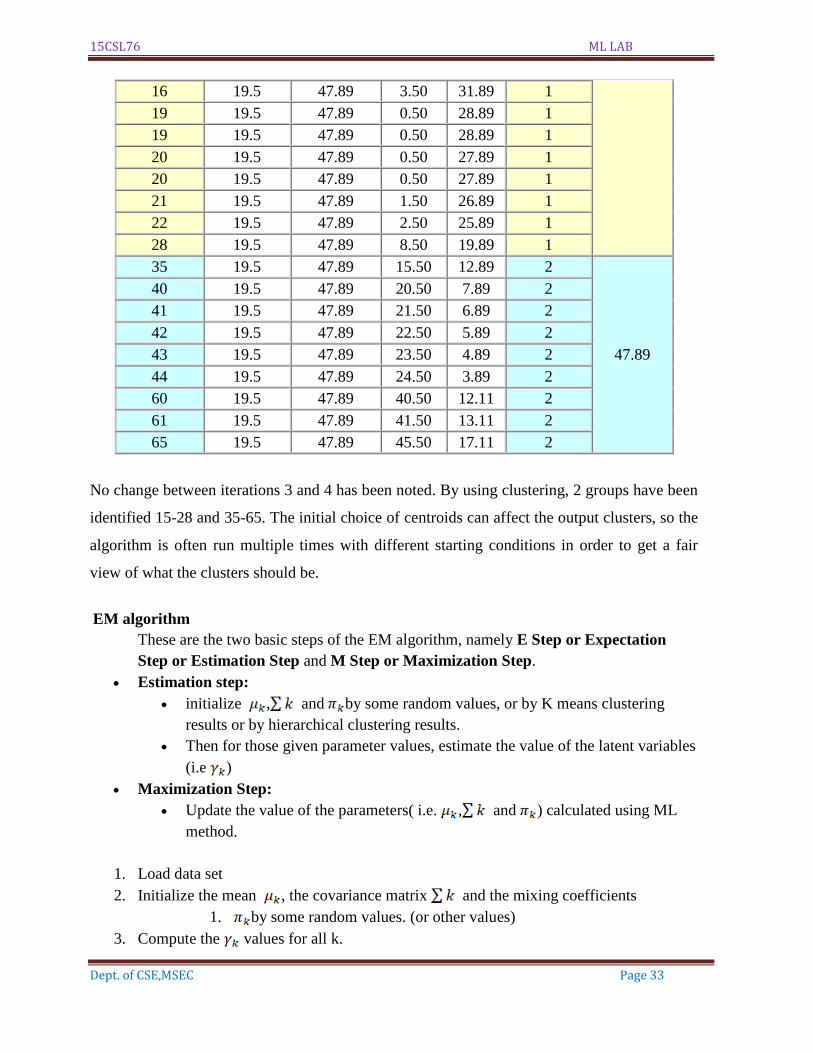
16 19.5 47.89 3.50 31.89 1

19 19.5 47.89 0.50 28.89 1

19 19.5 47.89 0.50 28.89 1

20 19.5 47.89 0.50 27.89 1

20 19.5 47.89 0.50 27.89 1

21 19.5 47.89 1.50 26.89 1

22 19.5 47.89 2.50 25.89 1

28 19.5 47.89 8.50 19.89 1

35 19.5 47.89 15.50 12.89 2

47.89

40 19.5 47.89 20.50 7.89 2

41 19.5 47.89 21.50 6.89 2

42 19.5 47.89 22.50 5.89 2

43 19.5 47.89 23.50 4.89 2

44 19.5 47.89 24.50 3.89 2

60 19.5 47.89 40.50 12.11 2

61 19.5 47.89 41.50 13.11 2

65 19.5 47.89 45.50 17.11 2

No change between iterations 3 and 4 has been noted. By using clustering, 2 groups have been

identified 15-28 and 35-65. The initial choice of centroids can affect the output clusters, so the

algorithm is often run multiple times with different starting conditions in order to get a fair

view of what the clusters should be.

EM algorithm

These are the two basic steps of the EM algorithm, namely E Step or Expectation

Step or Estimation Step and M Step or Maximization Step.

Estimation step:

initialize , and by some random values, or by K means clustering

results or by hierarchical clustering results.

Then for those given parameter values, estimate the value of the latent variables

(i.e )

Maximization Step:

Update the value of the parameters( i.e. , and ) calculated using ML

method.

1. Load data set

2. Initialize the mean , the covariance matrix and the mixing coefficients

1. by some random values. (or other values)

3. Compute the values for all k.

15CSL76 ML LAB


4. Again Estimate all the parameters using the current values.

5. Compute log-likelihood function.

6. Put some convergence criterion

7. If the log-likelihood value converges to some value ( or if all the parameters converge

to some values ) then stop, else return to Step 3.

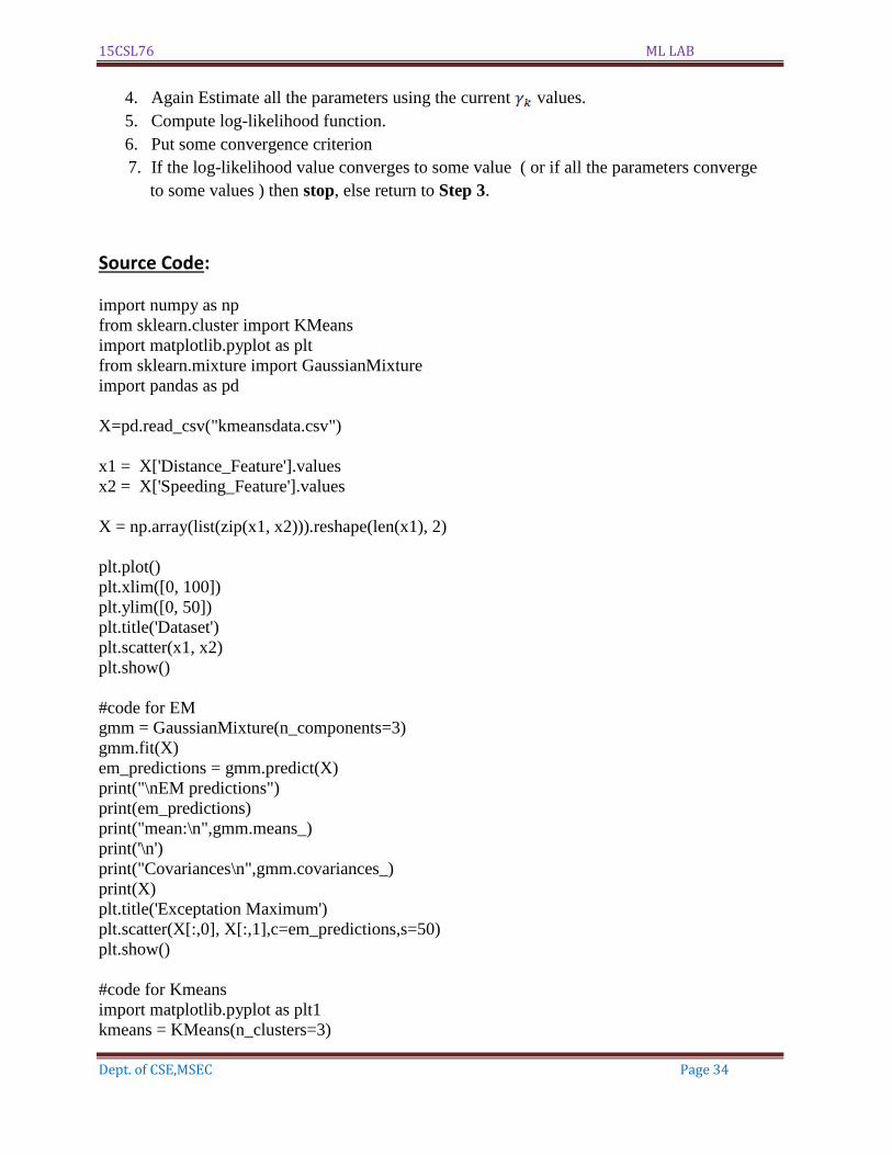
Source Code:

import numpy as np

from sklearn.cluster import KMeans

import matplotlib.pyplot as plt

from sklearn.mixture import GaussianMixture

import pandas as pd

X=pd.read_csv("kmeansdata.csv")

x1 = X['Distance_Feature'].values

x2 = X['Speeding_Feature'].values

X = np.array(list(zip(x1, x2))).reshape(len(x1), 2)

plt.plot()

plt.xlim([0, 100])

plt.ylim([0, 50])

plt.title('Dataset')

plt.scatter(x1, x2)

plt.show()

#code for EM

gmm = GaussianMixture(n_components=3)

gmm.fit(X)

em_predictions = gmm.predict(X)

print("\nEM predictions")

print(em_predictions)

print("mean:\n",gmm.means_)

print('\n')

print("Covariances\n",gmm.covariances_)

print(X)

plt.title('Exceptation Maximum')

plt.scatter(X[:,0], X[:,1],c=em_predictions,s=50)

plt.show()

#code for Kmeans

import matplotlib.pyplot as plt1

kmeans = KMeans(n_clusters=3)

15CSL76 ML LAB


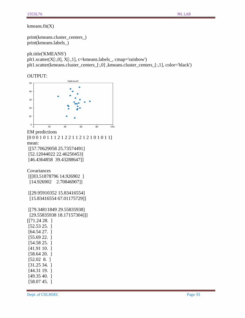
kmeans.fit(X)

print(kmeans.cluster_centers_)

print(kmeans.labels_)

plt.title('KMEANS')

plt1.scatter(X[:,0], X[:,1], c=kmeans.labels_, cmap='rainbow')

plt1.scatter(kmeans.cluster_centers_[:,0] ,kmeans.cluster_centers_[:,1], color='black')

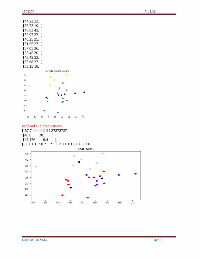
OUTPUT:

EM predictions

[0 0 0 1 0 1 1 1 2 1 2 2 1 1 2 1 2 1 0 1 0 1 1]

mean:

[[57.70629058 25.73574491]

[52.12044022 22.46250453]

[46.4364858 39.43288647]]

Covariances

[[[83.51878796 14.926902 ]

[14.926902 2.70846907]]

[[29.95910352 15.83416554]

[15.83416554 67.01175729]]

[[79.34811849 29.55835938]

[29.55835938 18.17157304]]]

[[71.24 28. ]

[52.53 25. ]

[64.54 27. ]

[55.69 22. ]

[54.58 25. ]

[41.91 10. ]

[58.64 20. ]

[52.02 8. ]

[31.25 34. ]

[44.31 19. ]

[49.35 40. ]

[58.07 45. ]

15CSL76 ML LAB


[44.22 22. ]

[55.73 19. ]

[46.63 43. ]

[52.97 32. ]

[46.25 35. ]

[51.55 27. ]

[57.05 26. ]

[58.45 30. ]

[43.42 23. ]

[55.68 37. ]

[55.15 18. ]

centroid and predications

[[57.74090909 24.27272727]

[48.6 38. ]

[45.176 16.4 ]]

[0 0 0 0 0 2 0 2 1 2 1 1 2 0 1 1 1 0 0 0 2 1 0]

15CSL76 ML LAB


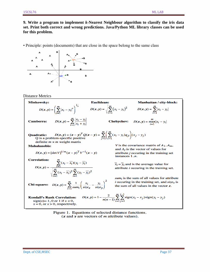
9. Write a program to implement k-Nearest Neighbour algorithm to classify the iris data

set. Print both correct and wrong predictions. Java/Python ML library classes can be used

for this problem.

• Principle: points (documents) that are close in the space belong to the same class

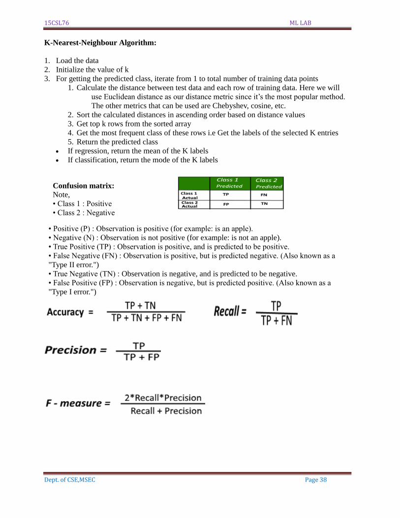
Distance Metrics

15CSL76 ML LAB


K-Nearest-Neighbour Algorithm:

1. Load the data

2. Initialize the value of k

3. For getting the predicted class, iterate from 1 to total number of training data points

1. Calculate the distance between test data and each row of training data. Here we will

use Euclidean distance as our distance metric since it’s the most popular method.

The other metrics that can be used are Chebyshev, cosine, etc.

2. Sort the calculated distances in ascending order based on distance values

3. Get top k rows from the sorted array

4. Get the most frequent class of these rows i.e Get the labels of the selected K entries

5. Return the predicted class

If regression, return the mean of the K labels

If classification, return the mode of the K labels

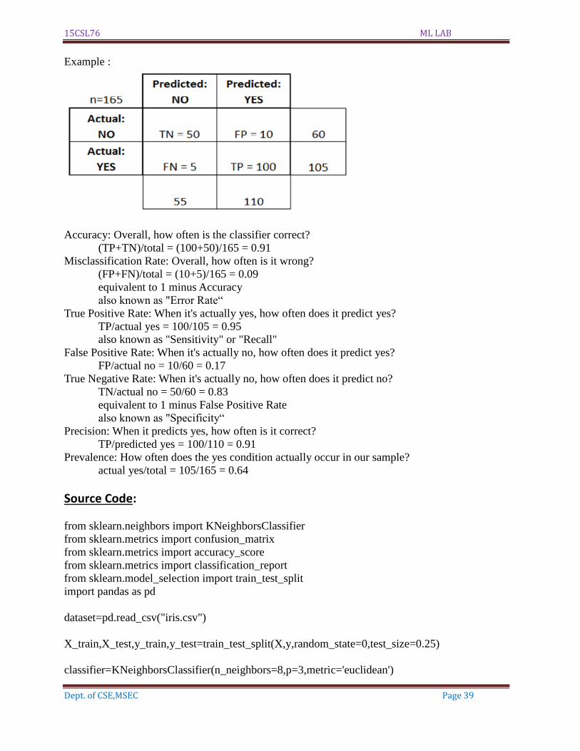
• Positive (P) : Observation is positive (for example: is an apple).

• Negative (N) : Observation is not positive (for example: is not an apple).

• True Positive (TP) : Observation is positive, and is predicted to be positive.

• False Negative (FN) : Observation is positive, but is predicted negative. (Also known as a

"Type II error.")

• True Negative (TN) : Observation is negative, and is predicted to be negative.

• False Positive (FP) : Observation is negative, but is predicted positive. (Also known as a

"Type I error.")

Confusion matrix:

Note,

• Class 1 : Positive

• Class 2 : Negative

15CSL76 ML LAB


Example :

Accuracy: Overall, how often is the classifier correct?

(TP+TN)/total = (100+50)/165 = 0.91

Misclassification Rate: Overall, how often is it wrong?

(FP+FN)/total = (10+5)/165 = 0.09

equivalent to 1 minus Accuracy

also known as "Error Rate“

True Positive Rate: When it's actually yes, how often does it predict yes?

TP/actual yes = 100/105 = 0.95

also known as "Sensitivity" or "Recall"

False Positive Rate: When it's actually no, how often does it predict yes?

FP/actual no = 10/60 = 0.17

True Negative Rate: When it's actually no, how often does it predict no?

TN/actual no = 50/60 = 0.83

equivalent to 1 minus False Positive Rate

also known as "Specificity“

Precision: When it predicts yes, how often is it correct?

TP/predicted yes = 100/110 = 0.91

Prevalence: How often does the yes condition actually occur in our sample?

actual yes/total = 105/165 = 0.64

Source Code:

from sklearn.neighbors import KNeighborsClassifier

from sklearn.metrics import confusion_matrix

from sklearn.metrics import accuracy_score

from sklearn.metrics import classification_report

from sklearn.model_selection import train_test_split

import pandas as pd

dataset=pd.read_csv("iris.csv")

X_train,X_test,y_train,y_test=train_test_split(X,y,random_state=0,test_size=0.25)

classifier=KNeighborsClassifier(n_neighbors=8,p=3,metric='euclidean')

15CSL76 ML LAB


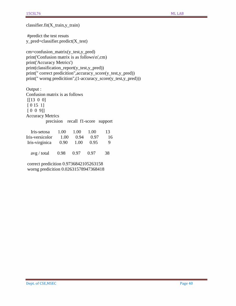
classifier.fit(X_train,y_train)

#predict the test resuts

y_pred=classifier.predict(X_test)

cm=confusion_matrix(y_test,y_pred)

print('Confusion matrix is as follows\n',cm)

print('Accuracy Metrics')

print(classification_report(y_test,y_pred))

print(" correct predicition",accuracy_score(y_test,y_pred))

print(" worng predicition",(1-accuracy_score(y_test,y_pred)))

Output :

Confusion matrix is as follows

[[13 0 0]

[ 0 15 1]

[ 0 0 9]]

Accuracy Metrics

precision recall f1-score support

Iris-setosa 1.00 1.00 1.00 13

Iris-versicolor 1.00 0.94 0.97 16

Iris-virginica 0.90 1.00 0.95 9

avg / total 0.98 0.97 0.97 38

correct predicition 0.9736842105263158

worng predicition 0.02631578947368418

15CSL76 ML LAB


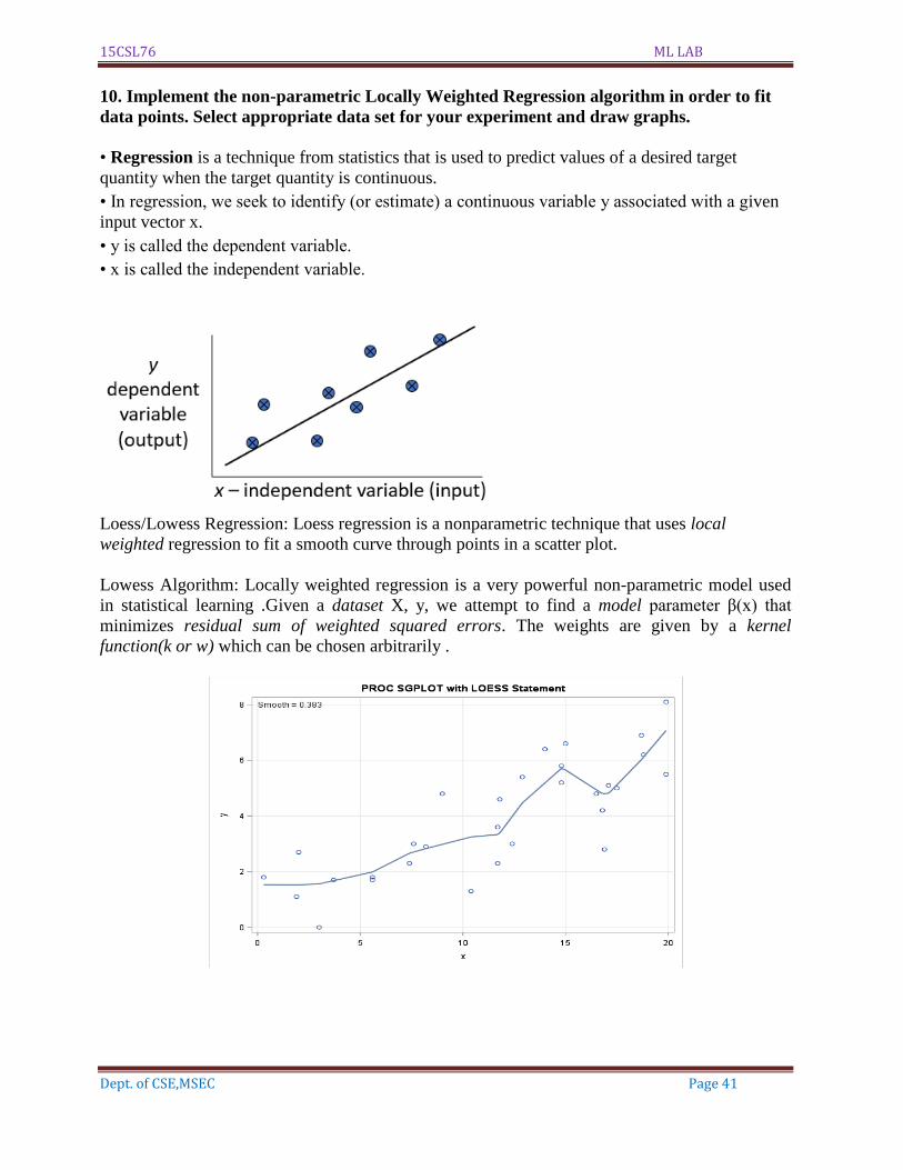
10. Implement the non-parametric Locally Weighted Regression algorithm in order to fit

data points. Select appropriate data set for your experiment and draw graphs.

• Regression is a technique from statistics that is used to predict values of a desired target

quantity when the target quantity is continuous.

• In regression, we seek to identify (or estimate) a continuous variable y associated with a given

input vector x.

• y is called the dependent variable.

• x is called the independent variable.

Loess/Lowess Regression: Loess regression is a nonparametric technique that uses local

weighted regression to fit a smooth curve through points in a scatter plot.

Lowess Algorithm: Locally weighted regression is a very powerful non-parametric model used

in statistical learning .Given a dataset X, y, we attempt to find a model parameter β(x) that

minimizes residual sum of weighted squared errors. The weights are given by a kernel

function(k or w) which can be chosen arbitrarily .

15CSL76 ML LAB


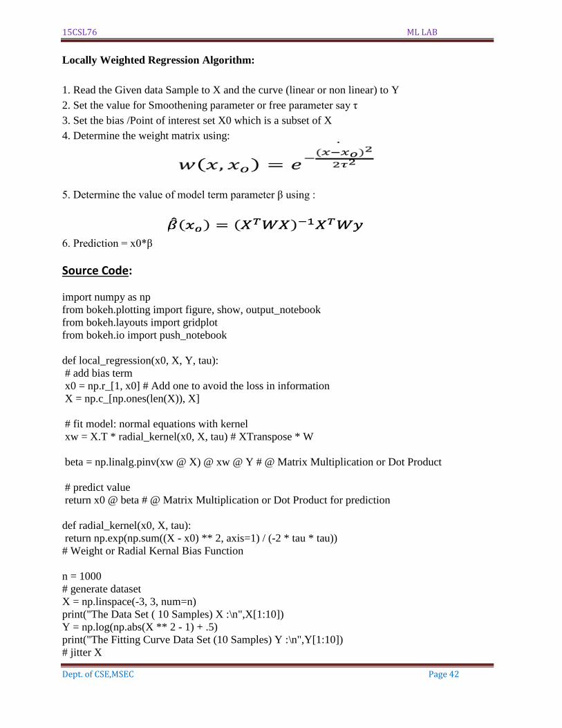
Locally Weighted Regression Algorithm:

1. Read the Given data Sample to X and the curve (linear or non linear) to Y

2. Set the value for Smoothening parameter or free parameter say τ

3. Set the bias /Point of interest set X0 which is a subset of X

4. Determine the weight matrix using:

5. Determine the value of model term parameter β using :

6. Prediction = x0*β

Source Code:

import numpy as np

from bokeh.plotting import figure, show, output_notebook

from bokeh.layouts import gridplot

from bokeh.io import push_notebook

def local_regression(x0, X, Y, tau):

# add bias term

x0 = np.r_[1, x0] # Add one to avoid the loss in information

X = np.c_[np.ones(len(X)), X]

# fit model: normal equations with kernel

xw = X.T * radial_kernel(x0, X, tau) # XTranspose * W

beta = np.linalg.pinv(xw @ X) @ xw @ Y # @ Matrix Multiplication or Dot Product

# predict value

return x0 @ beta # @ Matrix Multiplication or Dot Product for prediction

def radial_kernel(x0, X, tau):

return np.exp(np.sum((X - x0) ** 2, axis=1) / (-2 * tau * tau))

# Weight or Radial Kernal Bias Function

n = 1000

# generate dataset

X = np.linspace(-3, 3, num=n)

print("The Data Set ( 10 Samples) X :\n",X[1:10])

Y = np.log(np.abs(X ** 2 - 1) + .5)

print("The Fitting Curve Data Set (10 Samples) Y :\n",Y[1:10])

# jitter X

15CSL76 ML LAB


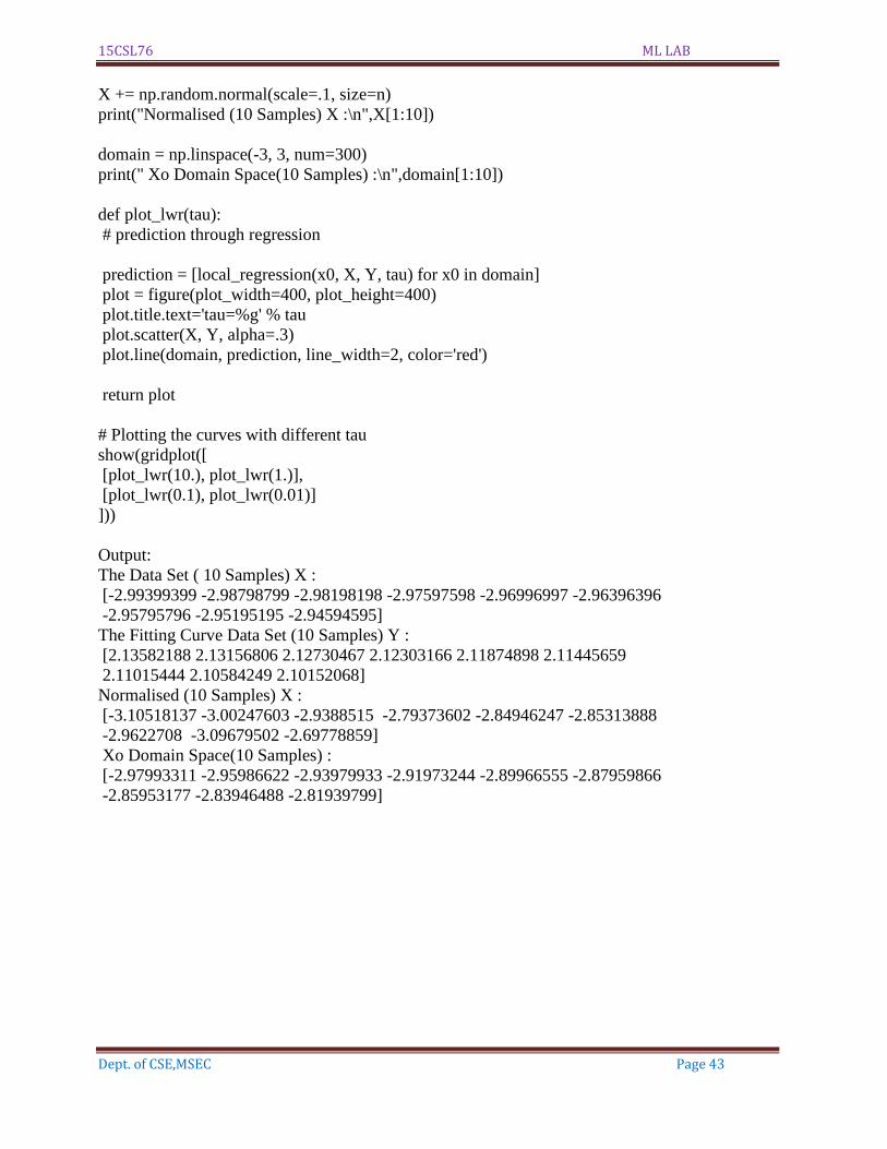
X += np.random.normal(scale=.1, size=n)

print("Normalised (10 Samples) X :\n",X[1:10])

domain = np.linspace(-3, 3, num=300)

print(" Xo Domain Space(10 Samples) :\n",domain[1:10])

def plot_lwr(tau):

# prediction through regression

prediction = [local_regression(x0, X, Y, tau) for x0 in domain]

plot = figure(plot_width=400, plot_height=400)

plot.title.text='tau=%g' % tau

plot.scatter(X, Y, alpha=.3)

plot.line(domain, prediction, line_width=2, color='red')

return plot

# Plotting the curves with different tau

show(gridplot([

[plot_lwr(10.), plot_lwr(1.)],

[plot_lwr(0.1), plot_lwr(0.01)]

]))

Output:

The Data Set ( 10 Samples) X :

[-2.99399399 -2.98798799 -2.98198198 -2.97597598 -2.96996997 -2.96396396

-2.95795796 -2.95195195 -2.94594595]

The Fitting Curve Data Set (10 Samples) Y :

[2.13582188 2.13156806 2.12730467 2.12303166 2.11874898 2.11445659

2.11015444 2.10584249 2.10152068]

Normalised (10 Samples) X :

[-3.10518137 -3.00247603 -2.9388515 -2.79373602 -2.84946247 -2.85313888

-2.9622708 -3.09679502 -2.69778859]

Xo Domain Space(10 Samples) :

[-2.97993311 -2.95986622 -2.93979933 -2.91973244 -2.89966555 -2.87959866

-2.85953177 -2.83946488 -2.81939799]

15CSL76 ML LAB


OR from numpy import *

import operator

from os import listdir

import matplotlib

import matplotlib.pyplot as plt

import pandas as pd

import numpy.linalg

from scipy.stats.stats import pearsonr

def kernel(point,xmat, k):

m,n = shape(xmat)

weights = mat(eye((m)))

for j in range(m):

diff = point - X[j]

weights[j,j] = exp(diff*diff.T/(-2.0*k**2))

return weights

def localWeight(point,xmat,ymat,k):

wei = kernel(point,xmat,k)

W = (X.T*(wei*X)).I*(X.T*(wei*ymat.T))

return W

def localWeightRegression(xmat,ymat,k):

m,n = shape(xmat)

ypred = zeros(m)

for i in range(m):

ypred[i] = xmat[i]*localWeight(xmat[i],xmat,ymat,k)

return ypred

# load data points

data = pd.read_csv('tips.csv')

bill = array(data.total_bill)

tip = array(data.tip)

15CSL76 ML LAB


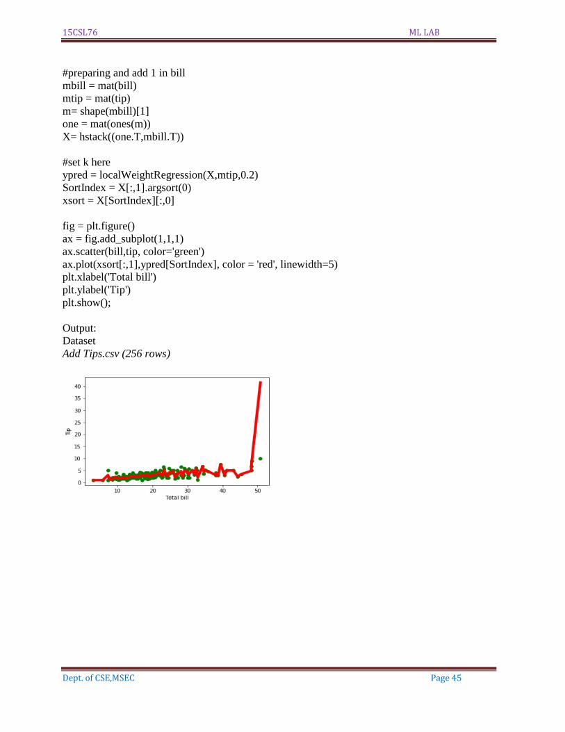
#preparing and add 1 in bill

mbill = mat(bill)

mtip = mat(tip)

m= shape(mbill)[1]

one = mat(ones(m))

X= hstack((one.T,mbill.T))

#set k here

ypred = localWeightRegression(X,mtip,0.2)

SortIndex = X[:,1].argsort(0)

xsort = X[SortIndex][:,0]

fig = plt.figure()

ax = fig.add_subplot(1,1,1)

ax.scatter(bill,tip, color='green')

ax.plot(xsort[:,1],ypred[SortIndex], color = 'red', linewidth=5)

plt.xlabel('Total bill')

plt.ylabel('Tip')

plt.show();

Output:

Dataset

Add Tips.csv (256 rows)

15CSL76 ML LAB


VIVA Questions

1. What is machine learning?

2. Define supervised learning

3. Define unsupervised learning

4. Define semi supervised learning

5. Define reinforcement learning

6. What do you mean by hypotheses?

7. What is classification?

8. What is clustering?

9. Define precision, accuracy and recall

10. Define entropy

11. Define regression

12. How Knn is different from k-means clustering

13. What is concept learning?

14. Define specific boundary and general boundary

15. Define target function

16. Define decision tree

17. What is ANN

18. Explain gradient descent approximation

19. State Bayes theorem

20. Define Bayesian belief networks

21. Differentiate hard and soft clustering

22. Define variance

23. What is inductive machine learning?

24. Why K nearest neighbor algorithm is lazy learning algorithm

25. Why naïve Bayes is naïve

26. Mention classification algorithms

27. Define pruning

28. Differentiate Clustering and classification

29. Mention clustering algorithms

30. Define Bias

31. What is learning rate? Why it is need.

ML Lab Manual.pdf - MS Engineering College

Documents

Transcript of ML Lab Manual.pdf - MS Engineering College