
A LABORATORY STUDY ON A SMALL GAS TURBINE
182
i ACOUSTIC EMISSION MONITORING OF PROPULSION SYSTEMS: A LABORATORY STUDY ON A SMALL GAS TURBINE Mohamad Shadi Nashed Submitted for the degree of doctor of philosophy on completion of research in the School of Engineering and Physical Sciences, Mechanical Engineering, Heriot-Watt University November 2010 This copy of the thesis has been supplied on condition that anyone who consults it is understood to recognise that the copyright rests with its author and that no quotation from the thesis and no information derived from it may be published without the prior written consent of the author or of the University (as may be appropriate).
-
Upload
khangminh22 -
Category
Documents
-
view
4 -
download
0
Transcript of A LABORATORY STUDY ON A SMALL GAS TURBINE

i
ACOUSTIC EMISSION MONITORING OF
PROPULSION SYSTEMS: A LABORATORY
STUDY ON A SMALL GAS TURBINE
Mohamad Shadi Nashed
Submitted for the degree of doctor of philosophy on completion of research in the School of Engineering and Physical Sciences, Mechanical Engineering,
Heriot-Watt University
November 2010
This copy of the thesis has been supplied on condition that anyone who consults it is
understood to recognise that the copyright rests with its author and that no quotation
from the thesis and no information derived from it may be published without the prior
written consent of the author or of the University (as may be appropriate).

ii
Abstract The motivation of the work is to investigate a new, non-intrusive condition monitoring
system for gas turbines with capabilities for earlier identification of any changes and the
possibility of locating the source of the faults. This thesis documents experimental
research conducted on a laboratory-scale gas turbine to assess the monitoring capabilities of
Acoustic Emission (AE). In particular it focuses on understanding the AE behaviour of
gas turbines under various normal and faulty running conditions.
A series of tests was performed with the turbine running normally, either idling or with
load. Two abnormal running configurations were also instrumented in which the
impeller was either prevented from rotation or removed entirely. With the help of
demodulated resonance analysis and an ANN it was possible to identify two types of AE; a
background broadband source which is associated with gas flow and flow resistance,
and a set of spectral frequency peaks which are associated with reverberation in the
exhaust and coupling between the alternator and the turbine.
A second series of experiments was carried out with an impeller which had been
damaged by removal of the tips of some of the blades (two damaged blades and four
damaged blades). The results show the potential capability of AE to identify gas turbine
blade faults. The AE records showed two obvious indicators of blade faults, the first
being that the energy in the AE signals becomes much higher and is distinctly periodic
at higher speeds, and the second being the appearance of particular pulse patterns which
can be characterized in the demodulated frequency domain.

iii
Acknowledgments
as ca rri e d out with � I would like to express my sincere gratitude to many individuals for their valuable
assistance during this work. However, it is difficult for me to list all the people who
encouraged and helped me during my studies and research. I apologise in advance for
any omissions.
Firstly, I wish to express my thanks to my supervisors, Professor Robert L. Reuben and
Professor John A. Steel for their invaluable supervision, guidance, and technical support
over the entire period of my Ph.D.
My thanks go to the mechanical and electronic technicians who have helped me to
manufacture and advised me on the test rigs and especially R. Kinsella.
I would also like to take this opportunity to express my appreciation to all those friends
and colleagues who made these years very memorable and extremely enjoyable and
especially Shadi, and Ghaleeh.
I am grateful to the Mechanical School at Aleppo University for the financial support.
Thanks are also due to my mum Hana, father, brothers, sisters, daughter Leen, and
especially my second mum Radwa for all her support.
Specially and most importantly, I would like to thank my lovely wife Marwa who
shared with me every moment in PhD period and supported me till the end with all her
great love and passion.

iv
Table of Contents Abstract ............................................................................................................................. ii
Acknowledgments ............................................................................................................ iii
Table of Contents ............................................................................................................. iv
Lists of Tables ................................................................................................................. vii
Lists of Figures............................................................................................................... viii
Nomenclature ................................................................................................................ xvii
Abbreviations ............................................................................................................... xviii
Chapter 1 Introduction ...................................................................................................... 1
1.1. Background to condition monitoring of gas turbines ............................................. 1
1.2. Aims and objectives: .............................................................................................. 3
1.3. Thesis outline ......................................................................................................... 4
1.4. Original contribution .............................................................................................. 5
Chapter 2 Literature Review ............................................................................................. 6
2.1. Introduction: ........................................................................................................... 6
2.2. Acoustic emission measurements: ......................................................................... 6
2.2.1. AE sources and waves: ................................................................................... 7
2.2.2. Attenuation: ..................................................................................................... 9
2.2.3. AE sensors and sensor calibration: .............................................................. 11
2.2.4. Practical implications of AE monitoring of machinery: ............................... 13
2.3. Acoustic emission analysis techniques: ............................................................... 16
2.3.1. AE features and extraction: .......................................................................... 16
2.3.2. Pattern recognition: ...................................................................................... 19
2.4. Condition monitoring and diagnostic systems: .................................................... 23
2.5. Acoustic emission for condition monitoring of turbines and machinery: ............ 27
2.6. Artificial neural networks in condition monitoring: ............................................ 31
2.7. Gas turbine faults: ................................................................................................ 33
2.8. Summary of state of knowledge and thesis identification: .................................. 39
Chapter 3 Experimental apparatus and procedures ......................................................... 40
3.1. Introduction: ......................................................................................................... 40
3.2. Apparatus: ............................................................................................................ 40
3.2.1. AE sensors and coupling: ............................................................................. 41
3.2.2. Preamplifiers: ............................................................................................... 42
3.2.3. Signal conditioning unit: ............................................................................... 43

v
3.2.4. Data acquisition (DAQ) system: ................................................................... 43
3.2.5. Simulated source for calibration and attenuation: ....................................... 44
3.2.6. Gas Turbine Rig: ........................................................................................... 45
3.3. Experimental procedure: ...................................................................................... 48
3.3.1. Turbine running tests: ................................................................................... 48
3.3.2. Damaged impeller tests: ............................................................................... 51
3.4. AE transmission and calibration tests: ................................................................. 52
3.4.1. Calibration tests on steel block:.................................................................... 53
3.4.2. Calibration test on gas turbine: .................................................................... 57
3.4.3. AE propagation on gas turbine:.................................................................... 61
Chapter 4 Results: normal running tests and tests without functioning impeller ........... 66
4.1. Turbine operation test without impeller ............................................................... 66
4.2. Test with jammed impeller .................................................................................. 74
4.3. Turbine operation test without load ..................................................................... 79
4.4. Turbine operation test with load .......................................................................... 85
4.5. Summary .............................................................................................................. 90
Chapter 5 Analysis and discussion of normal running tests ........................................... 92
5.1. Time domain analysis .......................................................................................... 92
5.1.1. Pulse shape categorisation ........................................................................... 92
5.1.2. Statistical time feature classification ............................................................ 98
5.2. Frequency domain analysis ................................................................................ 104
5.2.1. Raw frequency classification ...................................................................... 105
5.2.2. Demodulated frequency spectra.................................................................. 105
5.2.3. Demodulated frequency domain feature classification ............................... 110
5.3. Analysis combining time features and demodulated frequency features ........... 114
5.3.1. Pulse shape recognition combined with frequency features ....................... 114
5.3.2. Statistical time features combined with demodulated frequency features .. 116
5.4. Discussion of AE sources in the running turbine ............................................... 119
Chapter 6: Faulty impeller condition monitoring tests ................................................. 134
6.1. Results of tests with two damaged blades .......................................................... 134
6.2. Results of tests with four damaged blades ......................................................... 141
6.3. Discussion of damaged impeller tests ................................................................ 146
Chapter 7 Conclusion and future work ......................................................................... 150
7.1. Conclusions: ....................................................................................................... 150
7.2. Future work: ....................................................................................................... 153

vi
References ..................................................................................................................... 154
Appendix A: AE sensors calibration certificates .......................................................... 164

vii
Lists of Tables
Table 2. 1: Summary of typical statistical parameters used for continuous signals ....... 17
Table 3.1: Summary of Anova results comparing effects of variation in source with
variation in coupling for each sensor at each position. ................................................... 55
Table 3.2: Summary of Anova results comparing effects of variation in position with
variation in lead break, sensor and coupling at each position. ........................................ 56
Table 4. 1: Gas generator speed of without impeller test................................................ 67
Table 4. 2: Gas generator speed of without impeller test1.............................................. 72
Table 4. 3: Gas generator speed of jammed impeller test. .............................................. 74
Table 4. 4: Free power turbine speed of idling test. ........................................................ 79
Table 4. 5: Free power turbine speed of load test. .......................................................... 85
Table 4. 6: Average AE energy for both exhaust and shroud sensors of idling and load
tests.......................................................................................................................... 91
Table 5. 1: Thermo features of idling test. .................................................................... 132
Table 5. 2: Thermo features of load test. ...................................................................... 133

viii
Lists of Figures
Figure 2. 1: The main wave types: dilatational wave, and distortional wave and
Rayleigh wave (or surface wave). ..................................................................................... 9
Figure 2. 2: Schematic of an AE sensor, from Vallen [34]. ............................................ 12
Figure 2. 3: Attenuation example of AE signal on turbine rig. ....................................... 14
Figure 2. 4: Examples of attenuation characteristics on various cast iron structures (from
Nivesrangsan et al [38, 39]). ........................................................................................... 15
Figure 2. 5: Typical time domain features of AE signals ............................................... 18
Figure 2. 6: Demodulation of a lower-frequency signal by taking the envelope of the
raw AE. ........................................................................................................................... 19
Figure 2. 7: Example of AE energy of simulated damage to blades of free-power turbine
(from Douglas et al[78]). ................................................................................................ 28
Figure 2. 8: AE r.m.s. (V) activity during run-down of a 500 MW turbine (from
Zuluago-Giralda and Mba [80]). ..................................................................................... 29
Figure 2. 9: Boundary layer replica of a gas turbine blade. ............................................ 34
Figure 2. 10: Fracture surface of a blade with fatigue failure on the concave side near
trailing edge (TE: trailing edge; LE: leading edge) [103]. .............................................. 36
Figure 2. 11: Fracture surface of a blade with fatigue failure on the convex side near
trailing edge (TE: trailing edge; LE: leading edge) [103]. .............................................. 36
Figure 3.1: Schematic view of turbine rig and acoustic emission system. ..................... 40
Figure 3.2: Micro-80D broad band sensor. ..................................................................... 41
Figure 3.3: S9215 narrow band, high temperature sensor[119]. ..................................... 42
Figure 3.4: Preamplifier type PAC 1220A...................................................................... 43
Figure 3.5: Data acquisition system with accessories. .................................................... 44
Figure 3.6: Drawings and dimensions of standard (a) and modified (b) guide rings[120,
121] . ............................................................................................................................... 45
Figure 3.7: Schematic diagram of turbine rig showing positions of temperature and
pressure sensors............................................................................................................... 47
Figure 3.8: Photograph of turbine rig showing AE sensor positions. ............................. 47
Figure 3.9: Timing signal system .................................................................................... 48
Figure 3.10: Running test arrangement showing free power turbine with AE sensors and
power take-off belt. ......................................................................................................... 49
Figure 3.11: Schematic of dummy piece used to replace the impeller. .......................... 50
Figure 3.12: Free power turbine impeller with two damaged blades. ............................. 51

ix
Figure 3.13: Free power turbine impeller with four damaged blades. ............................ 52
Figure 3.14: (a) Overall schematic and (b) plan view of sensor positions on steel
calibration block. ............................................................................................................. 53
Figure 3.15: AE energy recorded at the three sensors on the steel block at four positions.
......................................................................................................................................... 54
Figure 3.16: Sensor 1 energy distribution for 10 placements at four positions; (a)
position 1, (b) position 2, (c) position 3, (d) position 4. ................................................. 55
Figure 3.17: Frequency domain of two AE sensor on steel block (a) Micro-80D
(exhaust) sensor, (b) S9215 (shroud) sensor. .................................................................. 57
Figure 3.18: Turbine sensor calibration arrangement showing sensor and AE source
positions. ......................................................................................................................... 58
Figure 3.19: AE energy calibration of S9215 sensor on turbine rig. .............................. 59
Figure 3.20: Histogram of AE energy for S9215 sensor calibration on turbine rig, (a)
before turbine operation, (b) after turbine operation (hot), (c) after turbine operation
(cold). .............................................................................................................................. 59
Figure 3. 21: AE energy calibration of Micro-80D sensor on turbine rig. ..................... 60
Figure 3. 22: Histogram of AE energy for Micro- 80D sensor calibration on turbine rig,
(a) before turbine operation, (b) after turbine operation (hot), (c) after turbine operation
(cold). .............................................................................................................................. 60
Figure 3.23: Turbine propagation test arrangement showing sensors and AE source
positions. ......................................................................................................................... 61
Figure 3.24: AE energy versus source-sensor distance with best-fit exponential decay
curve for S9215 sensor mounted on turbine shroud. ...................................................... 62
Figure 3.25: AE energy versus source-sensor distance with best-fit exponential decay
curve for Micro-80D sensor mounted on turbine shroud. ............................................... 63
Figure 3.26: AE energy versus source-sensor distance with best-fit exponential decay
curve for Micro-80D sensor on waveguide. .................................................................... 64
Figure 3.27: Micro-80D & S9215 sensor attenuation characteristics for sources on the
turbine surface. ................................................................................................................ 65
Figure 4.1: Typical Micro-80D AE signatures (exhaust) for test without impeller. Gas
generator speed increases from bottom to top, with S1 recorded at 500 RPS and S9
recorded at 1170 RPS. ..................................................................................................... 68
Figure 4.2: Typical S9215 AE signatures (shroud) for test without impeller. Gas
generator speed increases from bottom to top, with S1 recorded at 500 RPS and S9
recorded at 1170 RPS. ..................................................................................................... 68
x
Figure 4.3: Micro-80D (exhaust) sensor AE energy vs. gas generator speed for tests
without impeller. ............................................................................................................. 70
Figure 4.4: S9215 (shroud) sensor AE energy vs. gas generator speed for tests without
impeller. .......................................................................................................................... 70
Figure 4.5: Typical raw AE spectra for test without impeller: (a) Micro-80D sensor, (b)
S9215 sensor. Gas generator speed increases from bottom to top, with S1 recorded at
500 RPS and S9 recorded at 1170 RPS........................................................................... 71
Figure 4.6: Typical demodulated AE spectra for test without impeller with Micro-80D
sensor. Gas generator speed increases from bottom to top, with S1 recorded at 500 RPS
and S17 recorded at 1170 RPS. ....................................................................................... 73
Figure 4.7: Typical demodulated AE spectra for test without impeller with S9215
sensor. Gas generator speed increases from bottom to top, with S1 recorded at 500 RPS
and S17 recorded at 1170 RPS. ....................................................................................... 73
Figure 4.8: Typical Micro-80D AE signatures for jammed impeller test. Gas generator
speed increases from bottom to top, with S1 recorded at 500 RPS and S9 recorded at
850 RPS........................................................................................................................... 75
Figure 4.9: Typical S9215 AE signatures for jammed impeller test. Gas generator speed
increases from bottom to top, with S1 recorded at 500 RPS and S9 recorded at 850 RPS.
......................................................................................................................................... 75
Figure 4.10: Micro-80D (exhaust) sensor AE energy vs. gas generator speed for tests
jammed impeller. ............................................................................................................ 76
Figure 4.11: S9215 (shroud) sensor AE energy vs. gas generator speed for tests jammed
impeller. .......................................................................................................................... 76
Figure 4.12: Typical raw AE spectra for test jammed impeller: (a) Micro-80D sensor,
(b) S9215 sensor. Gas generator speed increases from bottom to top, with S1 recorded
at 500 RPS and S9 recorded at 850 RPS. ........................................................................ 77
Figure 4.13: Typical demodulated AE spectra for test with jammed impeller with
Micro-80D sensor. Gas generator speed increases from bottom to top, with S1 recorded
at 500 RPS and S9 recorded at 850 RPS. ........................................................................ 78
Figure 4.14: Typical demodulated AE spectra for test with jammed impeller with S9215
sensor. Gas generator speed increases from bottom to top, with S1 recorded at 500 RPS
and S9 recorded at 850 RPS. ........................................................................................... 78
Figure 4.15: Relationship between free power turbine speed and. gas generator speed for
idling test. ........................................................................................................................ 80

xi
Figure 4.16: Typical Micro-80D AE signatures (exhaust) for test without load. Free
power turbine speed increases from bottom to top, with S1 recorded at 140 RPS and S9
recorded at 345 RPS. ....................................................................................................... 80
Figure 4.17: Typical S9215 AE signatures (shroud) for test without load. Free power
turbine speed increases from bottom to top, with S1 recorded at 140 RPS and S9
recorded at 345 RPS. ....................................................................................................... 81
Figure 4.18: Micro-80D (exhaust) sensor AE energy vs. free power turbine speed for
tests without load. ........................................................................................................... 81
Figure 4.19: S9215 (shroud) sensor AE energy vs. free power turbine speed for tests
without load..................................................................................................................... 82
Figure 4.20: Typical raw AE spectra for test without load: (a) Micro-80D sensor, (b)
S9215 sensor. Free power turbine speed increases from bottom to top, with S1 recorded
at 140 RPS and S9 recorded at 345 RPS. ........................................................................ 83
Figure 4.21: Typical demodulated AE spectra for test without load with Micro-80D
sensor. Free power turbine speed increases from bottom to top, with S1 recorded at 140
RPS and S9 recorded at 345 RPS.................................................................................... 84
Figure 4.22: Typical demodulated AE spectra for test without load with S9215 sensor.
Free power turbine speed increases from bottom to top, with S1 recorded at 140 RPS
and S9 recorded at 345 RPS. ........................................................................................... 84
Figure 4.23: Typical Micro-80D AE signatures (exhaust) for test with load. Free power
turbine speed increases from bottom to top, with S1 recorded at 150 RPS and S9
recorded at 360 RPS. ....................................................................................................... 86
Figure 4.24: Typical S9215 AE signatures (shroud) for test with load. Free power
turbine speed increases from bottom to top, with S1 recorded at 150 RPS and S9
recorded at 360 RPS. ....................................................................................................... 86
Figure 4.25: Micro-80D (exhaust) sensor AE energy vs. free power turbine speed for
tests with load.................................................................................................................. 87
Figure 4.26: S9215 (shroud ) sensor AE energy vs. free power turbine speed for tests
with load. ......................................................................................................................... 87
Figure 4.27: Typical raw AE spectra for test with load: (a) Micro-80D sensor, (b)
S9215 sensor. Free power turbine speed increases from bottom to top, with S1 recorded
at 150 RPS and S9 recorded at 360 RPS. ........................................................................ 88
Figure 4.28: Typical demodulated AE spectra for test with load with Micro-80D sensor.
Free power turbine speed increases from bottom to top, with S1 recorded at 150 RPS
and S9 recorded at 360 RPS. ........................................................................................... 89
xii
Figure 4.29: Typical demodulated AE spectra for test with load with S9215 sensor. Free
power turbine speed increases from bottom to top, with S1 recorded at 150 RPS and S9
recorded at 360 RPS. ....................................................................................................... 89
Figure 5.1: The four characteristic pulse signatures identified from Micro-80D signals.
......................................................................................................................................... 93
Figure 5.2: The four characteristic pulse signatures identified from S9215 signals. ...... 93
Figure 5.3: Artificial neural network structure for pulse shape recognition. .................. 94
Figure 5.4: Example ANN recognition performance for AE signatures of Micro-80D
(exhaust) for unseen signatures from idling test. ............................................................ 94
Figure 5.5: Sample coded signal for pulse shape recognition of Micro-80D (exhaust)
sensor for idling test. ....................................................................................................... 95
Figure 5.6: Pulse shape recognition ANN performance for Micro-80D (exhaust) data
from idling tests. ............................................................................................................. 96
Figure 5.7: Pulse shape recognition ANN performance for S9215 (shroud) data from
idling tests. ...................................................................................................................... 96
Figure 5.8: Improved pulse shape recognition ANN performance for Micro-80D
(exhaust) data from idling tests. ...................................................................................... 97
Figure 5.9: improved pulse shape recognition ANN performance for S9215 (shroud)
data from idling tests. ...................................................................................................... 97
Figure 5.10: ANN classification performance using all statistical time features: (a)
S9215 sensor, idling tests, (b) Micro-80D sensor, idling tests, (c) S9215 sensor, load
tests, (d) Micro-80D sensor, load tests. ........................................................................... 99
Figure 5.11: ANN speed estimate error for S9215 sensor idling test. .......................... 100
Figure 5.12: ANN speed estimate error for Micro-80D sensor on idling test. ............. 100
Figure 5.13: ANN speed estimate error for S9215 sensor on load test. ........................ 101
Figure 5.14: ANN speed estimate error for Micro-80D sensor on load test. ................ 101
Figure 5.15: ANN performance for individual time features derived from idling test: (a)
S9215 sensor,(b) Micro-80D sensor. ............................................................................ 102
Figure 5.16: ANN performance for individual time features derived from without load
test: (a) S9215 sensor,(b) Micro-80D sensor. ............................................................... 102
Figure 5.17: Cumulative ANN performance for time features in idling test: (a) S9215
sensor, (b) Micro-80D sensor. ....................................................................................... 103
Figure 5.18: Cumulative ANN performance for time features in load test: (a) S9215
sensor, (b) Micro-80D sensor. ....................................................................................... 104
xiii
Figure 5.19: ANN performance for without load tests of frequency features (a) Micro-
80D sensor performance (b) S9215 sensor performance. ............................................. 105
Figure 5.20: Demodulated spectra for idling test with Micro-80D sensor at 8 different
speeds of FPT. Individual spectra shown in blue and averaged spectra shown in red. 107
Figure 5.21:Demodulated spectra for idling test with S9215 sensor at 8 different speeds
of FPT. Individual spectra shown in blue and averaged spectra shown in red. ............ 108
Figure 5.22: Demodulated spectra for load test with Micro-80D sensor at 8 different
speeds of FPT. Individual spectra shown in blue and averaged spectra shown in red. 109
Figure 5.23: Demodulated spectra for load test with S9215 sensor at 8 different speeds
of FPT. Individual spectra shown in blue and averaged spectra shown in red. ............ 110
Figure 5. 24: (a) S9215 without load tests, (b) Micro-80D sensor without load tests, (c)
S9215 sensor with load tests, (d) Micro-80D sensor with load tests. ........................... 111
Figure 5.25: ANN speed estimate error for S9215 sensor on idling test. ..................... 112
Figure 5.26: ANN speed estimate error for Micro-80D sensor on idling test. ............. 112
Figure 5.27 : ANN speed estimate error for S9215 sensor on load test. ....................... 113
Figure 5.28: ANN speed estimate error for Micro-80D sensor on load test. ................ 113
Figure 5.29: Pulse shape recognition ANN performance for idling tests including raw
frequency features (a) Micro-80D sensor performance (b) S9215 sensor performance.
....................................................................................................................................... 115
Figure 5. 30: Pulse shape recognition ANN performance for idling tests including
demodulated frequency features (a) Micro-80D sensor performance (b) S9215 sensor
performance. ................................................................................................................. 115
Figure 5.31: ANN performance with time and frequency features: (a) S9215 sensor
without load tests, (b) Micro-80D sensor without load tests, (c) S9215 sensor with load
tests, (d) Micro-80D sensor with load tests................................................................... 116
Figure 5.32: ANN error for S9215 sensor during without load test. ............................ 117
Figure 5.33: ANN error for Micro-80D sensor during without load test. ..................... 117
Figure 5.34: ANN error for S9215 sensor during with load test................................... 118
Figure 5.35: ANN error for Micro-80D sensor during with load test. .......................... 118
Figure 5.36: Shroud sensor spectral peaks energy removal for idling tests. (Blue points
before removing energy and the red points after) ......................................................... 120
Figure 5.37: Exhaust sensor spectral peaks energy removal idling tests. (Blue points
before removing energy and the red points after) ......................................................... 120
Figure 5.38: Shroud sensor spectral peaks removal load tests. (Blue points before
removing energy and the red points after) .................................................................... 121

xiv
Figure 5.39: Exhaust sensor spectral peaks removal load tests. (Blue points before
removing energy and the red points after) .................................................................... 121
Figure 5. 40: Shroud sensor background AE energy for idling, jammed, without
impeller tests. ................................................................................................................ 122
Figure 5.41: Exhaust sensor background AE energy for idling, jammed, without
impeller tests. ................................................................................................................ 122
Figure 5.42: Shroud sensor background AE energy for idling and load tests. ............. 123
Figure 5.43: Exhaust sensor background AE energy for idling and load tests. ............ 123
Figure 5.44: Shroud sensor energy fraction of spectral peaks frequencies for idling test1.
....................................................................................................................................... 124
Figure 5.45: Shroud sensor energy fraction of spectral peaks frequencies of idling test2.
....................................................................................................................................... 125
Figure 5.46: Shroud sensor energy fraction of spectral peaks frequencies of idling test3.
....................................................................................................................................... 125
Figure 5.47: Exhaust sensor energy fraction of spectral peaks frequencies of idling test1.
....................................................................................................................................... 126
Figure 5.48: Exhaust sensor energy fraction of spectral peaks frequencies of idling test2.
....................................................................................................................................... 126
Figure 5.49: Exhaust sensor energy fraction of spectral peaks frequencies of idling test3.
....................................................................................................................................... 127
Figure 5.50: Shroud sensor energy fraction of spectral peaks frequencies for load test1.
....................................................................................................................................... 128
Figure 5.51: Shroud sensor energy fraction of spectral peaks frequencies for load test2.
....................................................................................................................................... 128
Figure 5.52: Shroud sensor energy fraction of spectral peaks frequencies for load test3.
....................................................................................................................................... 129
Figure 5.53: Exhaust sensor energy fraction of spectral peaks frequencies for load test1.
....................................................................................................................................... 129
Figure 5.54: Exhaust sensor energy fraction of spectral peaks frequencies for load test2.
....................................................................................................................................... 130
Figure 5.55: Exhaust sensor energy fraction of spectral peaks frequencies for load test3.
....................................................................................................................................... 130
Figure 5.56: Schematic of gas turbine exhaust system. ................................................ 131

xv
Figure 6.1: Typical Micro-80D AE signatures (exhaust) for test with two damaged
blades. Free power turbine speed increases from bottom to top, with S1 recorded at 95
RPS and S9 recorded at 325 RPS.................................................................................. 135
Figure 6.2: Typical S9215 AE signatures (shroud) for test with two damaged blades.
Free power turbine speed increases from bottom to top, with S1 recorded at 95 RPS and
S9 recorded at 325 RPS. ............................................................................................... 135
Figure 6.3: Micro-80D (exhaust) sensor AE energy vs. free power turbine speed for test
with two damaged blades. ............................................................................................. 136
Figure 6.4: S9215 (shroud) sensor AE energy vs. free power turbine speed for test with
two damaged blades. ..................................................................................................... 136
Figure 6.5: Typical raw AE spectra for test with two damaged blades: (a) Micro-80D
sensor, (b) S9215 sensor. Free power turbine speed increases from bottom to top, with
S1 recorded at 95 RPS and S9 recorded at 325 RPS. ................................................... 138
Figure 6.6: Demodulated spectra for test with two damaged blades with Micro-80D
sensor at 8 different speeds of FPT. .............................................................................. 139
Figure 6.7 : Demodulated spectra for test with two damaged blades with S9215 sensor
at 8 different speeds of FPT. ......................................................................................... 140
Figure 6.8: Typical Micro-80D AE signatures (exhaust) for test with four damaged
blades. Free power turbine speed increases from bottom to top, with S1 recorded at 110
RPS and S8 recorded at 385 RPS.................................................................................. 141
Figure 6.9: Micro-80D (exhaust) sensor AE energy vs. free power turbine speed for test
with four damaged blades. ............................................................................................ 142
Figure 6.10: S9215 (shroud) sensor AE energy vs. free power turbine speed for test with
four damaged blades. .................................................................................................... 142
Figure 6.11: Typical raw AE spectra for test with four damaged blades: (a) Micro-80D
sensor, (b) S9215 sensor. Free power turbine speed increases from bottom to top, with
S1 recorded at 110 RPS and S8 recorded at 385 RPS. ................................................. 143
Figure 6.12: Demodulated spectra for test with four damaged blades with Micro-80D
sensor at 8 different speeds of FPT. .............................................................................. 144
Figure 6.13: Demodulated spectra for test with four damaged blades with S9215 sensor
at 8 different speeds of FPT. ......................................................................................... 145
Figure 6. 14: AE signature recorded on shroud for test with two damaged blades. .... 147
Figure 6.15: Demodulated frequency graph from shroud AE signature for test with two
damaged blades. ............................................................................................................ 147
Figure 6.16: AE signature recorded on exhaust for test with four damaged blades. ... 148

xvi
Figure 6.17: Demodulated frequency graph for exhaust AE signature for test with four
damaged blades. ............................................................................................................ 149

xvii
Nomenclature a Attenuation coefficient (dB/m) γ adiabatic index of gas r Density (kg/m3) s Standard deviation
iA , iA1 , iA2 Amplitude of AE signal (dB or V)
rA Relative amplitude (dB) C sound speed in gas (m/sec) E Energy content (V2.s) ( )xE Energy at distance, x (V2.s)
oE Energy of the source (V2.s) Fcrit Variance within the group Fvalue Variance between the group f the reverberating frequency (Hz). k Attenuation factor or Attenuation coefficient ( 1-m ) Kurt Kurtosis M molar mass in kilograms per mole P1-P4 Sensor positions R molar gas constant (J·mol−1·K−1) rms RMS energy at each window Skew Skewness S1-9 Turbine running speed(RPS) t Time (s) ( )tv Amplitude of signal (V)
Var Variance x Distance (m)
xviii
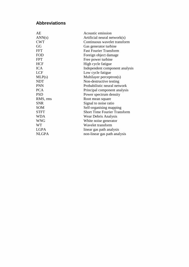
Abbreviations AE Acoustic emission ANN(s) Artificial neural network(s) CWT Continuous wavelet transform GG Gas generator turbine FFT Fast Fourier Transform FOD Foreign object damage FPT Free power turbine HCF High cycle fatigue ICA Independent component analysis LCF Low cycle fatigue MLP(s) Multilayer perceptron(s) NDT Non-destructive testing PNN Probabilistic neural network PCA Principal component analysis PSD Power spectrum density RMS, rms Root mean square SNR Signal to noise ratio SOM Self-organising mapping STFT Short Time Fourier Transform WDA Wear Debris Analysis WNG White noise generator WT Wavelet transform LGPA linear gas path analysis NLGPA non-linear gas path analysis

1
Chapter 1 Introduction This work relates to the condition monitoring of turbines using acoustic emission (AE).
A small, laboratory-scale turbine has been instrumented using AE sensors and
recordings made of the AE as a function of position on the machine for various normal
operating conditions and fault conditions, as well as for some idealized conditions to
understand the source of AE in the machine. This chapter introduces the technological
background and significance of the work as well as presenting the motivation for the
research.
1.1. Background to condition monitoring of gas turbines The application of condition monitoring techniques to machinery allows earlier
diagnosis and prompt repair of any malfunction and avoidance of breakdown caused by
faulty components, which is its most critical use for process plant and machinery.
Moreover, condition monitoring systems can be used to identify the machine condition
in order to achieve economic performance through increased availability and reduced
component replacement costs through predictive maintenance. Generally the main
methods which have been developed for condition monitoring of gas turbines are
performance analysis[1], oil analysis [2], and vibration analysis [3].
Performance analysis is widely used on rotating machines, and specifically on gas and
steam turbines. Performance analysis is based on the idea that any deterioration in the
machine will produce changes in the operating parameters from their ideal values [4].
The combination of performance analysis with other artificial intelligence techniques
constitutes a good tool for providing information about the degradation severity of the
machine components. One of the limitations is that measurement quality has a critical
influence on the reliability of a performance analysis condition monitoring system, and
most measured data are contaminated by sensor noise, disturbances, instrument
degradation, and human error to a greater or lesser extent.
Wear Debris Analysis (WDA) involves examining the debris suspended in lubricating
oil in order to predict machine condition [5]. One drawback of this technique is that it is
inappropriate for certain machines and/or operations, such as electrical machinery and
switch gear, which can be monitored by acoustic emission and ultrasonic techniques.

2
Another disadvantage of WDA is the difficulty of applying it to sealed systems where
obtaining a sample of fluid is difficult and usually not recommended. A further demerit
is the inability to identify the precise location of the fault and several faults from
different components can cause confusion. Finally, the necessary analysis is normally
performed in batches in a laboratory rendering it not particularly amenable to
continuous or on-line monitoring. The most prominent advantage of WDA is that it
directly diagnoses wear, which is not usually achievable economically using other
techniques.
Vibration analysis [6] is one of the most widely applied condition monitoring
techniques for rotating and reciprocating machines. Generally, vibration analysis starts
by drawing a comparison between historical measurements and recent values using
some kind of trending. A wide range of features are conventionally extracted from the
recorded signals from the time domain, the frequency domain, and the quefrency
domain [7]. Vibration signals are sensitive to low frequency environmental noise such
as machine resonances or ancillary equipment. Aِlthough, the vibration method is
indirect but it has the potential benefit of source location.
The above techniques including performance analysis, oil analysis, and vibration
monitoring are all indirect in that they measure the changes in some aspect of the
machine operation from which an attempt is made to deduce condition. Furthermore,
these approaches are generally unable to give information about the exact locations of
changes in the turbine. Acoustic Emission (AE) sources include impacts, wear, crack
propagation and gas flow all of which can occur in gas turbine operation. As a non
intrusive technique, AE has two potential advantages over other techniques; (a) its
ability of early identification of any changes, (b) the potential to locate the source of the
emission [8]. Acoustic emission (AE) has been used successfully for condition
monitoring of machinery and has proven to be a useful tool for monitoring a number of
rotating machinery types such as gas turbines, steam turbines, and pumps. Detailed
reported examples include the diagnosis of faults on the inner and outer races of gas
turbine bearings [9, 10], rubbing and bearing damage in a steam turbine [11], the
transmissibility of acoustic emission across very large-scale turbine rotors[12], and
detecting cavitation in pumps [13].

3
1.2. Aims and objectives: Turbine engines are extremely difficult to monitor with high operating temperatures and
huge centrifugal speeds and loads. They are subject to a range of failure mechanisms
which might be expected to modify the flow through the machine. AE has been used
successfully for machinery monitoring in lower speed rotating machines, reciprocating
engines, bearings, fuel injection and combustion, where the fundamental sources are
similar to those expected in a gas turbine. Therefore using AE to monitor gas turbine
engines to enable classification of the operating parameters and fault diagnosis is the
main aim of this research.
The detailed aims are therefore:
1. To understand the fundamental mechanisms generating AE signals in gas
turbines.
2. To study the effect of operating conditions on AE signals and develop
recognition approaches.
3. To identify potential benefits of AE monitoring over conventional turbine
monitoring approaches.
4. To demonstrate the potential of AE technique for diagnosing gas turbine blade
defects.
To pursue these aims, the following objectives were set:
1. Calibrate AE sensors on a standard steel block and on gas turbine rig.
2. Study AE propagation characteristics in the gas turbine rig.
3. Categorize the AE signatures under various normal running conditions of the gas
turbine.
4. Understand and explain the complex AE behavior of gas turbine during normal
operation.
5. Simulate various blade defects and characterize the AE signature in time and
frequency domains.

4
1.3. Thesis outline This thesis is organized in 7 chapters, the contents of which are summarized as follows. Chapter 1: Introduction
This chapter introduces the general background of condition monitoring of gas turbines
and the place of AE monitoring in this context. The objectives of the research and the
claimed contribution to knowledge are also identified.
Chapter 2: Literature review
This chapter describes the general physics of AE wave propagation including wave
types, wave propagation speed, effects of AE wave attenuation, AE sensor calibration
procedures, and AE analysis techniques in the time and frequency domains. The main
part of the chapter is a critical review of condition monitoring methods on gas turbines
and other machinery with emphasis on the advanced diagnostic methods used for fault
monitoring of gas turbines. The AE application with advanced diagnostic methods on
gas turbine has been reviewed in this chapter. A summary of common gas turbine faults
is also included in this chapter.
Chapter 3: Experimental apparatus and procedures
This chapter describes the experimental apparatus, data acquisition methods,
experimental set-up and experimental procedure for the laboratory tests of AE
calibration on steel block, AE calibration on the gas turbine, AE propagation on the gas
turbine, as well as monitoring the gas turbine under various operating conditions with
and without simulated impeller faults. The results of the calibrations and attenuation
tests are also summarized here.
Chapter 4: Results: normal running tests and tests without functioning impeller
This chapter shows the results of simple time- and frequency-domain analyses of four
different test configurations; idling with the speed being controlled by fuel and air flow,
or under load at fixed fuel and air flow as well as two abnormal running tests in which
the impeller was either prevented from rotating or removed entirely.
Chapter 5: Analysis and discussion of normal running tests
This chapter extends the preliminary analysis of chapter 4 in order to explain the
complex AE behavior in the gas turbine for the idling and load tests. Pattern recognition

5
techniques using artificial neural networks have been applied to aid the understanding of
the characteristics of AE behaviour of gas turbine.
Chapter 6: Faulty impeller condition monitoring tests
The results of the tests conducted on with a faulty free power turbine are described in
this chapter. These are analysed using time- and frequency-domain processing to
indicate how pulse train analysis can be used to track blade faults in turbines.
Chapter 7: Conclusions and future work
The main findings and achievements of this research are detailed here along with
recommendations for possible future studies.
1.4. Original contribution
The overall outcome of improved monitoring capabilities of gas turbine processes based
upon analysis of AE signals is the specific area in which a contribution to knowledge is
claimed. As far as the author is aware, detailed study on the complex pattern recognition
of acoustic emission from gas turbines using artificial neural network has not previously
been attempted. Furthermore, the study has developed and used a technique based on
the demodulated frequency analysis to diagnose gas turbine blade faults. Some success
is claimed also in identifying the fluid-mechanical sources of the AE in turbines which
is of generic interest to turbine and machinery monitoring.

6
Chapter 2 Literature Review
2.1. Introduction: This chapter aims at providing a summary of the state of knowledge of the areas
relevant to the condition monitoring of gas turbines using AE. Condition monitoring is
here considered to be any tool for providing an assessment of machinery condition
based on collecting sensor data, and interpreting it with regard to any deterioration that
could affect machine life. A successful monitoring system will have the potential to
minimise the cost of maintenance, improve operational safety, and reduce the incidence
of in-service machine failure or breakdown.
The review is divided into six parts, commencing with an outline of how engineering
AE measurements are made, followed by a critical discussion of the conventional
analysis approaches. Next the role of other condition monitoring techniques such as
vibration monitoring, performance analysis, and oil analysis in gas turbines is evaluated
in preparation for a comparison of their strengths and weaknesses compared with what
is currently known about AE monitoring of turbines. In view of its relevance to this
work, a summary of the use of artificial neural networks in condition monitoring is
provided. Finally in this chapter, the range of commonly-encountered gas turbine faults
is explained with a view to identifying those which might reasonably be monitored
using AE.
2.2. Acoustic emission measurements: The term acoustic emission (AE) is normally reserved to describe high frequency stress
waves generated on the surface or within a material. The stress wave propagates in, or
on, the material and can be detected externally by mounting a sensor on an appropriate
surface. The degree to which one or more sensors can be used to determine the
characteristics of the source depends on a number of factors, such as AE wave
propagation, AE attenuation, and AE sensor calibration, as well as a number of practical
issues, all of which are discussed in this section.

7
2.2.1. AE sources and waves:
Sources of AE can be categorized as fundamental material sources and pseudo
sources[14]. Crack growth, slip, twinning and phase transformation are examples of the
first type, while pseudo sources include phenomena which give rise to the fundamental
sources, such as leaks [15], mechanical impact [16], sliding contact, turbulent fluid
flow, fluid cavitation [17], wear and friction[18]. Apart from crack growth, all of the
sources of potential interest in turbines are in the latter category and this is common to
most machinery monitoring applications.
AE sources can also be categorized depending on the type of signals they produce,
which can be either discrete or continuous. A single burst of energy produced by a
fracture or an impact leads to a discrete signal, whereas sources occurring rapidly to the
extent that they overlap in time and/or continuous sources lead to a continuous or quasi-
continuous signal. Examples of the latter are the AE signals associated with such
phenomena as fluid flow, fluid leaks, some chemical processes and sleeve bearings.
AE sources can further be categorised in terms of how they are stimulated, (a) structural
testing where a load is applied for the purpose of inspection, (b) process monitoring, for
example of machines such as engines, turbines and rotating machines, (c) materials
testing where the AE is used as a diagnostic of material behavior.
In the monitoring application, AE can be regarded as passive ultrasound, i.e. the AE
events are self-generated and the recorded ultrasound is not the result of a pulse or wave
injected into the component as occurs in ultrasonic non-destructive testing. One of the
oft-cited advantages of AE is its ability to reveal faults at an early stage, giving an
opportunity for intervention before sudden failure [19]. The reason this is essentially
that AE is generally sensitive to the processes that cause degradation as opposed to the
symptoms of degradation having occurred, one example being that AE can detect
bearing wear processes as opposed to, say, acceleration monitoring which might be
more sensitive to the looseness arising from excessive wear having occurred.
When an AE signal is generated by a source, the stress waves (approximate frequency
range of 100 kHz to 1.2 MHz) radiate and propagate to the boundaries of the structure
where they may be dissipated or reflected back into the structure, depending on the

8
nature of the structure, particularly the material and the size and shape. At any point on
a surface, arriving waves may have suffered refraction, scattering, and attenuation [20]
and may have been reflected once or more from boundaries, all of which makes
interpretation difficult.
AE waves propagate in solid media in one or more of four classes: longitudinal waves,
shear waves, Rayleigh waves and Lamb waves [21, 22]. The wave modes [23]
constitute a complete orthogonal set of eigenfunctions, which is to say that each one
propagates independently without losing energy to the other. Longitudinal and shear
waves are plane waves and are the only ones which propagate in infinite media. The
particle movement in the longitudinal wave in isotropic materials is parallel to the
direction of wave propagation but in shear waves it is perpendicular (Figure 1.1).
Longitudinal waves are faster than shear waves because the elastic modulus is greater
with that kind of deformation. Rayleigh waves propagate in media considered to be
semi-infinite and require a free surface. The velocity is a little lower than a shear wave
and the particles move in ellipses. Lamb waves are plane waves in an infinite medium
and the particles move in ellipses during its propagation [22]. The Lamb wave velocity
varies with frequency, a phenomenon known as velocity dispersion [21, 22, 24]. There
are two families of Lamb waves which are essentially coupled surface waves,
symmetric (often called extensional waves) (s0) and asymmetric (often called flexural
waves) (a0). Both wave modes propagate at various speeds, which are dependent on
both frequency and plate thickness. The extensional mode has a lower amplitude than
the flexural component and occurs as a small amplitude precursor to the larger flexural
wave. In practical situations, the AE energy is carried in one or more mode and each
mode can be converted to another at a boundary. It is not common to treat AE waves as
pure modes and, for many applications (including the current one), the AE can be
treated as a packet of mixed frequency propagating at a specific group velocity.

9
Compression Extension
Direction of wave propagation
Wavelength (l)
Direction ofparticle motion
(a) Dilatational wave (Longitudinal wave)
Shear deformation region
Direction of wave propagation
Wavelength (l)
Direction ofparticle motion
(b) Distortional wave (Shear wave)
Wavelength (l)
Direction of wave propagation
Direction of particle motion
Wavelength (l)
Direction of wave propagation
Direction of particle motion
(c) Rayleigh wave or surface wave
Figure 2. 1: The main wave types: dilatational wave, and distortional wave and Rayleigh wave (or surface wave).
2.2.2. Attenuation:
AE waves are subject to attenuation during their propagation inside a material [14, 25,
26], which manifests itself as a loss of amplitude as a wave propagates. There are four
main mechanisms of attenuation:
· Geometric spreading of the wave with constant energy whereby the amplitude of
the wave decreases with increasing distance from the source
· Wave dispersion, in which the shape of the pulse changes as it propagates
· Scattering and diffraction which are manifest as a decrease in amplitude when
waves encounter medium boundaries such as holes, slots, cavitation bubbles,

10
inclusions and cracks. Scattering occurs when the AE waves propagate through
the finite void or inclusion, while diffraction occurs when AE waves propagate
at edges, whereas some of the energy of the propagated wave through these
boundaries will scatter or diffract.
· Internal friction, which is due to the damping capacity of the material itself [27,
28]. Internal friction dominates [22] the attenuation in the far field and can be
described by an exponential relationship for amplitude with distance, giving
much steeper attenuation close to the source. In plates and shells, the transition
distance at which internal friction starts to dominate over geometric spreading is
given by 4.34/ α, where α is a (measured) attenuation factor (dB/m) [22].
Graham and Alers [29] have measured attenuation of AE waves on various structures
such as steel, aluminum and alumina ceramic plates, and a large pressure vessel using a
white noise generator (WNG) as an AE source. The AE signals were acquired at various
distances from the source then the loss in amplitude as a function of distance was
obtained using equation 2.2. They found that attenuation on the large pressure vessel
follows the expected form for geometrical spreading and varies with 1/ r in the near-
field zone. In the far-field zone, the attenuation of the signal is caused by absorption
with a limited amount of dispersion. Holford and Carter [27], working with long,
structural steel I-beams, found that the attenuation of waves was sharpest in the near-
field zone at around 10 dB over 0.5 m (20 dB/m) and lower for longer source-sensor
distances (1 dB/m). They attributed the higher attenuation in the near-field zone to
geometric spreading, and that in the far-field zone to absorption or conversion of AE
wave energy into heat. Prosser [30] found that the larger effect on the flexural waves on
a graphite/epoxy composite plate were attenuated more than extensional waves and
attributed the greater attenuation to dispersion. McIntire [14] used a simple power law
to describe AE attenuation in steel tubes:
0A A xa= (2.1)
Where A is the signal amplitude at a distance, x, from the source and A0 is the amplitude
of the source. He found that the exponent, α, for steel tube of 150 mm diameter was for
8.1 dB/m the near field and 1.9 dB/m for the far field. Shehadeh et al [31] estimated
automatically the arrival times of two AE components, a fast and a slow component,
using an array of sensors on a steel pipe. Their technique relied upon the balance of
high- and low-frequency components of the signal as a function of time to determine

11
arrival time. They applied three techniques i.e. cross correlation, wavelet transform,
filtering technique, and found that the best technique was cross correlation which
located the source with error less than 3%.
2.2.3. AE sensors and sensor calibration:
Acoustic emission (AE) is a passive non-destructive testing (NDT) technique that has
been used widely since the 1970s. Generally the stress wave arrives at the sensor at a
frequency in the approximate range of 100 kHz to 1.2 MHz with surface elevations in
the nm range. AE sensors [32] are mechanical-electrical transducers which convert this
mechanical disturbance to an electrical signal, and, in this sense, the measurement is
indirect. Furthermore, the AE signal measured at the sensor will be influenced by the
sensor’s response to the forcing transient waves, which is, in turn, influenced by the sensor
construction, including the piezoelectric properties of the sensing element as well as its size,
shape and backing, which govern the amplitude sensitivity and associated self-resonance.
As well as this, the propagation path from source to sensor and the nature of the coupling
between the sensor and the surface will affect what is recorded.
The successful use of piezoelectric AE sensors in industry over other transduction
technologies such as capacitive, electromagnetic and laser-optical measurement comes
from the fact that AE sensors have proven to be sufficiently sensitive and robust to be
used in a variety of environments. The material most often used for the active element in
piezoelectric AE sensors is lead zirconate titanate (PZT), although it has been shown that
other piezo-active materials such as quartz and even polymers like polyvinylidene
diflouride (PVDF) are equally feasible [33]. Figure 2.2 shows a schematic diagram of a
typical AE sensor. For AE sensors, there is always a compromise between bandwidth
and sensitivity, i.e. when the bandwidth of the application is known to be narrow then a
higher sensitivity can be achieved by adjusting the geometry of the piezoelectric element.
However, if a broad bandwidth is needed such as for machinery monitoring, the sensitivity
of the sensor over the range will be lower. Commercial AE sensors are sensitive to
frequencies above 100 kHz, whereas resonant sensors in the region of 150 kHz to 300
kHz are probably the most widely used in AE applications. The highest frequencies
likely to be of interest to users of AE transducers are in the range of 800 kHz to 1.2
MHz and transducers with bandwidths which extend above this range are not normally
used. Analogue band-pass filters are essential with AE systems to ensure that electronic
12
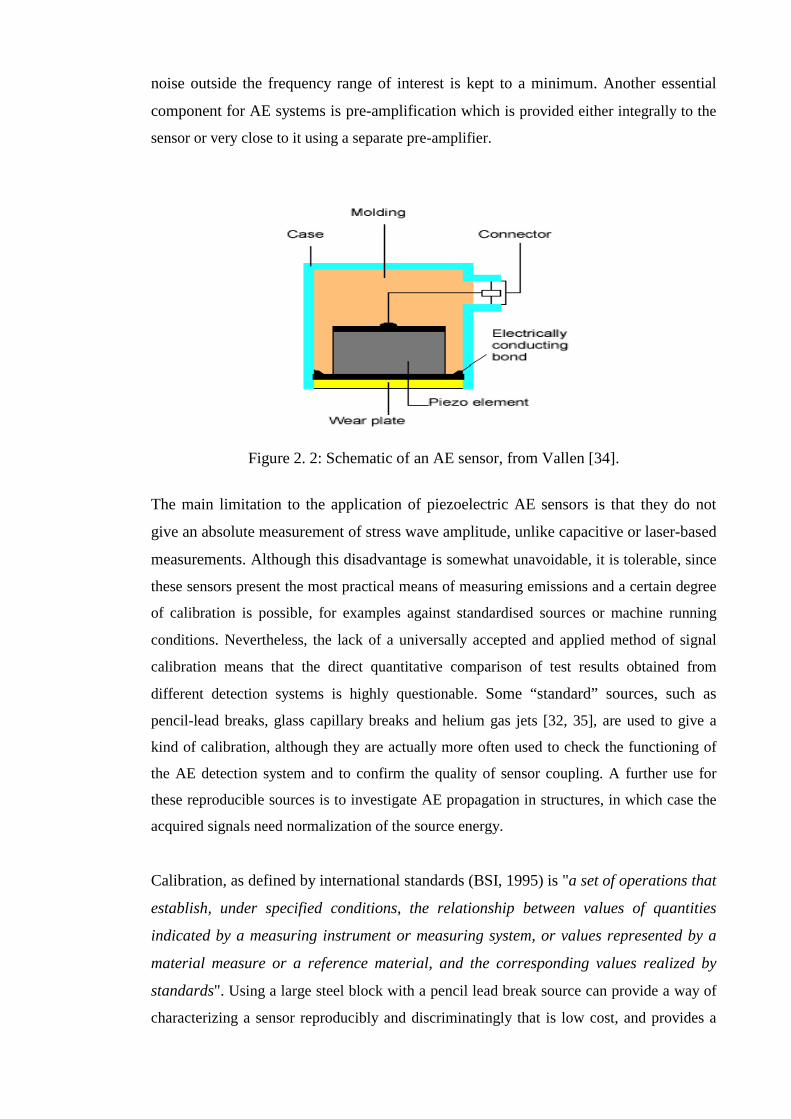
noise outside the frequency range of interest is kept to a minimum. Another essential
component for AE systems is pre-amplification which is provided either integrally to the
sensor or very close to it using a separate pre-amplifier.
Figure 2. 2: Schematic of an AE sensor, from Vallen [34].
The main limitation to the application of piezoelectric AE sensors is that they do not
give an absolute measurement of stress wave amplitude, unlike capacitive or laser-based
measurements. Although this disadvantage is somewhat unavoidable, it is tolerable, since
these sensors present the most practical means of measuring emissions and a certain degree
of calibration is possible, for examples against standardised sources or machine running
conditions. Nevertheless, the lack of a universally accepted and applied method of signal
calibration means that the direct quantitative comparison of test results obtained from
different detection systems is highly questionable. Some “standard” sources, such as
pencil-lead breaks, glass capillary breaks and helium gas jets [32, 35], are used to give a
kind of calibration, although they are actually more often used to check the functioning of
the AE detection system and to confirm the quality of sensor coupling. A further use for
these reproducible sources is to investigate AE propagation in structures, in which case the
acquired signals need normalization of the source energy.
Calibration, as defined by international standards (BSI, 1995) is "a set of operations that
establish, under specified conditions, the relationship between values of quantities
indicated by a measuring instrument or measuring system, or values represented by a
material measure or a reference material, and the corresponding values realized by
standards". Using a large steel block with a pencil lead break source can provide a way of
characterizing a sensor reproducibly and discriminatingly that is low cost, and provides a

13
very simple calibration [36]. Such a test can confirm the uniformity of a set of nominally
identical sensors used in a given lab or provide a cross-calibration between different sensors
used for the same task. If carefully specified, the test can also be used to compare AE data
from different tests in different laboratories, using different instrumentation.
2.2.4. Practical implications of AE monitoring of machinery: In general, the structures of machines such as gas turbines will consist of a number of
parts of varying geometric complexity, some joints and other features, such as webs and
welds. In addition, the internal surfaces may be in contact with oil or hot gases. AE
wave propagation will therefore be much more complex than simpler plate- and block-
like structures. Some authors such as Miller and McIntire[14], Pollock [22] and Kolsky
[37], have suggested an approach to studying the attenuation in such complex
structures by acquiring AE signals at different positions relative to a source. Thereafter,
the attenuation is described by using peak amplitude and a logarithmic relative
amplitude scale, ( Ar ) [22, 27, 29] :
÷÷ø
öççè
æ=
0
log.20A
AA i
r (2.2)
where Ai is the maximum signal amplitude (V) at a receiver sensor at distance x from
the source, and A0 is the maximum signal amplitude (V) at the source position.
The amplitudes can be measured in volts provided that the amplifiers are consistently
calibrated. Then, wave attenuation can be determined from a plot of the relative
amplitude versus distance and can be expressed as decibels per unit distance [14],
determined by:
x
A
A
A
xr=÷÷
ø
öççè
æ=
1
2log.20
a (2.3)
where α is attenuation coefficient (dB/m)
A1 is amplitude of signal at a position P1 (V)
A2 is amplitude of signal at a position P2 (V) and;
x is distance between P1 and P2 (m)
14
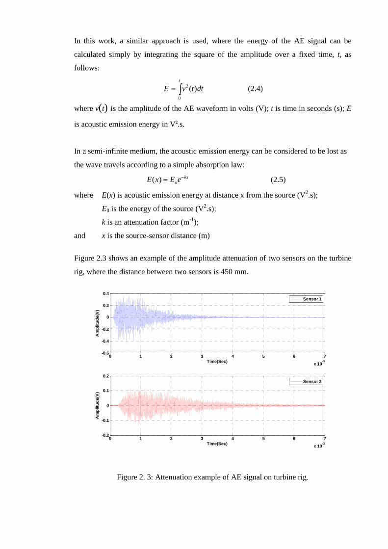
In this work, a similar approach is used, where the energy of the AE signal can be
calculated simply by integrating the square of the amplitude over a fixed time, t, as
follows:
dttvEt
)(0
2ò= (2.4)
where v(t) is the amplitude of the AE waveform in volts (V); t is time in seconds (s); E
is acoustic emission energy in V2.s.
In a semi-infinite medium, the acoustic emission energy can be considered to be lost as
the wave travels according to a simple absorption law:
kxoeExE -=)( (2.5)
where E(x) is acoustic emission energy at distance x from the source (V2.s);
E0 is the energy of the source (V2.s);
k is an attenuation factor (m-1);
and x is the source-sensor distance (m)
Figure 2.3 shows an example of the amplitude attenuation of two sensors on the turbine
rig, where the distance between two sensors is 450 mm.
0 1 2 3 4 5 6 7
x 10-3
-0.6
-0.4
-0.2
0
0.2
0.4
Time(Sec)
Am
plit
ud
e(V
)
0 1 2 3 4 5 6 7
x 10-3
-0.2
-0.1
0
0.1
0.2
Time(Sec)
Am
plit
ud
e(V
)
Sensor 2
Sensor 1
Figure 2. 3: Attenuation example of AE signal on turbine rig.
15
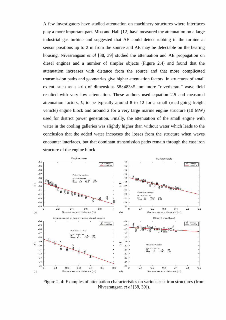
A few investigators have studied attenuation on machinery structures where interfaces
play a more important part. Mba and Hall [12] have measured the attenuation on a large
industrial gas turbine and suggested that AE could detect rubbing in the turbine at
sensor positions up to 2 m from the source and AE may be detectable on the bearing
housing. Nivesrangsan et al [38, 39] studied the attenuation and AE propagation on
diesel engines and a number of simpler objects (Figure 2.4) and found that the
attenuation increases with distance from the source and that more complicated
transmission paths and geometries give higher attenuation factors. In structures of small
extent, such as a strip of dimensions 58×483×5 mm more “reverberant” wave field
resulted with very low attenuation. These authors used equation 2.5 and measured
attenuation factors, k, to be typically around 8 to 12 for a small (road-going freight
vehicle) engine block and around 2 for a very large marine engine structure (10 MW)
used for district power generation. Finally, the attenuation of the small engine with
water in the cooling galleries was slightly higher than without water which leads to the
conclusion that the added water increases the losses from the structure when waves
encounter interfaces, but that dominant transmission paths remain through the cast iron
structure of the engine block.
Figure 2. 4: Examples of attenuation characteristics on various cast iron structures (from
Nivesrangsan et al [38, 39]).

16
2.3. Acoustic emission analysis techniques: For processing purposes, it is conventional to class AE signals as of burst type or
continuous type, although some acknowledge a mixture of the two. In the first kind, the
signal consists of clearly defined ‘events’ characterized by amplitudes significantly larger
than the background level, while the continuous kind occurs when burst generation is so
rapid that the resolution of individual events is not possible. Obviously, this basic
distinction has a fundamental bearing on the type of analysis that is used.
The analysis technique used can also depend on the application itself. For some
applications statistical time domain analysis to extract time-based features is sufficient,
while, for other applications, frequency domain analysis is needed. In some cases
simple time and frequency domain analysis is not adequate requiring the use of higher-
level analysis techniques such as artificial neural networks, fuzzy logic and expert
systems.
2.3.1. AE features and extraction: Extracting time features from raw AE signals is considered a first level of signal
processing. Normally, time features are used to describe characteristics of time series
data from random, stationary, ergodic and continuous processes. Table 2.1 summarises
a typical set of time-based features that might be used for continuous signals.

17
Feature Summary description Maximum value (
maxx ) - Indicates the maximum value of discrete time series data
Minimum value ( minx ) - Indicates the minimum value of discrete time series data
Mean value ( x ) or the first moment of amplitude distribution function
å=
=N
iix
Nx
1
1 (2.6)
where N is the number of data points; and
ix is the data at each discrete point in time.
- Measures the central distribution of discrete time series data.
Root mean square (RMS) value
N
xrms
N
iiå
== 1
2
(2.7)
- Measures square root of mean square in discrete time series data. - Indicates energy contained in continuous AE data.
Variance (Var ) or the second moment of the amplitude distribution function.
[ ]å=
-==N
ii xx
NVar
1
22 1s (2.8)
- Indicates the spread or dispersion or distribution of discrete time series data.
Standard deviation (s )
[ ]å=
-=N
ii xx
N 1
2 1s (2.9)
- Indicates the spread or dispersion or distribution of discrete time series data.
Skewness ( Skew ) or the third moment of amplitude distribution function
å=
úûù
êëé -
=N
i
i xxN
Skew1
3 1
s (2.10)
- Measures the lack of symmetry of distribution of discrete time series data. - 0=Skew represents normal distribution - For, 0<Skew the left tail of distribution is heavier than the right tail and opposite for. 0>Skew
Kurtosis ( Kurt ) or the fourth moment of amplitude distribution function.
å=
-úûù
êëé -
=N
i
i xxN
Kurt1
4 3 1
s (2.11)
- Measures the degree of peakedness of distribution of discrete time series data. - 0>Kurt represents a peaked distribution. - 0<Kurt represents a flat distribution. - 0=Kurt represents normal distribution.
Table 2. 1: Summary of typical statistical parameters used for continuous signals
For discontinuous (burst) signals, a specific set of features have evolved. These include:
· the AE event count, which is the number of times that the burst signal crosses a
preset threshold
· the AE event rate, which is the time rate at which AE event counts occur
· the AE count or ringdown count is the number of times the burst signal
amplitude exceeds the preset threshold
· the count rate, which is the number of AE counts per unit time

18
0 1 2 3 4 5 6
x 10-3
-1.5
-1
-0.5
0
0.5
1
1.5
Time(Sec)
Am
plit
ud
e(V
)
0 1 2 3 4 5 6
x 10-3
0
1
2
3
4
Time(Sec)
Am
plit
ud
e(V
2 )
6 6.2 6.4 6.6 6.8 7
x 10-4
0
0.1
0.2
0.3
0.4
0.5
Time(Sec)
Am
plit
ud
e(V
)
0 1 2 3 4 5 6
x 10-3
0
0.1
0.2
0.3
0.4
0.5
Time(Sec)
Am
plit
ud
e(V
)
RMSCounts
Max Amp
Threshold
Duration
Rise time
Figure 2. 5: Typical time domain features of AE signals
Frequency analysis depends on decomposing the time series signal into the frequency
domain., most commonly done using a Fast Fourier Transform (FFT) algorithm [40]. The
FFT algorithm can be used to estimate the distribution of the signal energy in the
frequency domain, using the Power Spectral Density (PSD) and Welch’s PSD estimate [41].
Frequency analysis can be used in machinery fault diagnosis as part of an approach which
uses known repeat times to filter out effects, such as running speed, and resonance, from
those of unknown origin for normal and faulty conditions. Furthermore, some sources of
AE can be masked by noise and filtering can again be used to separate the noise from the
signal, thus enhancing the signal-to-noise ratio. Dealing with non-stationary signals, such as
AE, where frequency can vary substantially with time, techniques such as the Short Time
Fourier Transform (STFT),which combines time and frequency analysis, can be used [42].
This implements the FFT algorithm at time increments throughout the signal using a sliding
window approach. Other methods for time-frequency analysis include wavelet
decomposition [43-46]. The wavelet transform is a powerful method that analyses the
signal using multi-scaling where the resolution of time and frequency vary in the time-
frequency plane. Longer time intervals give more precise low frequency information
and shorter time intervals give high frequency information. Therefore, a high resolution
of time frequency representation can be obtained[46].
One further application of the FFT of particular use for rotating machinery is called
demodulated resonance analysis [47]. The technique involves averaging the signal to reveal

19
lower frequencies in the envelope of the signal in a similar way to AM radio, where the AE
wave acts as a carrier frequency for the lower frequency information, Figure 2.6.
0 0.005 0.01 0.015 0.02 0.025 0.03-0.5
0
0.5
1
Time(sec)
Am
plit
ud
e(V
)
Raw signal
0 0.005 0.01 0.015 0.02 0.025 0.030
0.1
0.2
0.3
0.4
0.5
0.6RMS of raw signal
Time(sec)
Am
plit
ud
e(V
)0 1 2 3 4 5
x 105
0
0.5
1
1.5
2
2.5
3x 10
-7
Frequency(Hz)
Am
plit
ud
e(V
)
FFT of raw signal
0 500 1000 1500 20000
0.005
0.01
0.015
Frequency(Hz)
Am
plit
ud
e(V
)
FFT of RMS
RMS
Figure 2. 6: Demodulation of a lower-frequency signal by taking the envelope of the raw AE.
2.3.2. Pattern recognition: Pattern recognition is "the act of taking in raw data and taking an action based on the
category of the pattern"[48]. The sensor type(s), feature extraction mechanism, and
classification scheme are the main components of a pattern recognition system, in that
the sensors are normally the main source of observations and sensor data is transferred
to the feature extraction mechanism to describe the essential elements of the data. The
final stage depends on the classification scheme which organizes the features into
clusters using a classification algorithm.
The normal statistical approaches to AE analysis are helpful in many cases, but can
become unwieldy for complex pattern recognition cases such as for generic or real time
monitoring requirements involving large amounts of data and adaptability to new
situations. Pattern recognition therefore forms the basis of machine intelligence and AE,
with its sensitivity to a wide range of physical phenomena, can clearly play a major role
there.
Because of the high sampling rates and consequently high time resolution, AE
monitoring normally generates a large set of data. To handle the data, it is therefore

20
helpful to use some form of data reduction to prepare the variables for further statistical
classification and diagnostic algorithms. Principal component analysis (PCA) [49, 50],
is one such higher-level statistical analysis technique, involving a mathematical
procedure that transforms a number of (possibly) correlated variables into a (smaller)
number of uncorrelated variables called principal components in order to identify new
meaningful underlying variables and to reduce the dimensionality of the data.
An extension of the PCA technique is Independent Component Analysis (ICA), which
is also a higher statistical technique mainly used for decomposing a complex dataset
into independent sub-parts [51, 52]. In other words, it is a signal isolation technique
which works by assuming that the source signals are non-Gaussian, statistically
independent and hidden under the main signal. ICA is suitable for many fields,
including digital images, document databases, economic indicators and signal
processing. It helps provide good representation of multivariate data for reasons of
computational and conceptual simplicity.
Fuzzy logic [53] is an approach which simulates the human capability of imprecise
reasoning by providing a remarkably simple way to draw definite conclusions from
vague, ambiguous or imprecise information. It is very effective for the complex nature
of mechanical condition monitoring systems. Fuzzy logic [54] systems usually consist
of a fuzzifier, which maps crisp input numbers into fuzzy groups characterized by
linguistic variables and membership functions, an inference engine which decides the
way in which the fuzzy sets are combined, and a defuzzifier which produces a scholar
number into the output of the fuzzy logic system. Fuzzy logic demonstrates a good
ability to simulate the human imprecise reasoning [55], but it involves time-consuming
processing of the data and so is often combined with other techniques such as expert
systems, genetic algorithms, and neural networks to achieve good monitoring and fault
diagnostic systems. Neuro-Fuzzy networks accomplish this need by combining fuzzy
logic system with neural networks to combine the advantages of fuzzy logic with the
learning and adaptation capabilities of neural networks.
An expert system is a computer program, normally categorized as a type of artificial
intelligence, which performs functions similarly to a human expert [56, 57]. Building
any expert system needs a knowledge engineer or "knowledge base", a coding system to
translate how human experts make decisions into a simpler computer programming

21
language, and the user interface. The declaration of a fault by the coding system is
normally done by comparing engine component deviations with predefined thresholds
in the knowledge base. There are many types of expert systems such as case-based,
modal-based, and rule-based, which is considered the most popular system. Expert
systems have been used as a diagnostic tool for many kinds of aero-engines such as the
T53 and TF-34 jet engines, and twin engine gas turbines from a helicopter [58, 59].
Doel [60] concluded that expert system technologies were not going to make jet engine
diagnostic and maintenance procedures ‘smart’, but they could add a lot of new
capability that will make them more effective and more convenient. A recent
development of expert systems is a hybrid version where probability theory, fuzzy
logic, and belief functions are used to increase the diagnostic accuracy of the system
[61].
An Artificial Neural Network (ANN) is a mathematical model that is inspired by the
biological nervous system. Neural networks are structured in layers of interconnecting
processing elements (neurons), with the behavior of the network being determined by
the weights associated with each connection. These weights can be adaptively trained
using example signals to associate a particular input pattern to an output classification.
In other words [62] an artificial neural network is actually a massively parallel
distributed processor made up of simple processing units (neurons), which have a
natural propensity for storing experimental knowledge and making it available for use.
Artificial neural networks generally can be classified into two kinds: supervised and
unsupervised neural networks. Feed-Forward-Back-Propagation Networks [57] are
considered to be the most popular type of supervised neural network where the
information propagates from input to output while calculated errors propagate in the
opposite direction. In supervised neural networks a set of inputs (x) and outputs (y) are
used to build a function that matches the input with the output using iterative training.
Next the trained network, with the weights of its neurons adjusted to recognize the
output vector, is used to predict the value of the output for any valid new input vector.
Normally the training is validated tested against a set of “unseen” training data.
Unsupervised neural networks work with an input only to find patterns in data, and
classify it into clusters. The most popular learning method for unsupervised neural
networks is the competitive method, which consists of two phases, the first of which
identifies the winner neurons while the second updates the connection weights of the
winner neurons. For engine diagnostics the main unsupervised neural networks used

22
are; probabilistic neural networks PNN, self-organizing maps SOM, and learning vector
quantization LVQ. PNNs [63] classify the training patterns to classes and, when an
unknown pattern is input to the network, calculate the Euclidean distances between the
stored pattern and input pattern and then convert them, depending on the density
function, where the smallest distance has the highest probability and vice versa. PNN
application is suitable for smooth classification problems. In an SOM [4], the network is
like a lattice with the neurons located at its nodes. The statistical features of input
patterns and the spatial locations of the neurons determine the tuned neurons. Then
these neurons will form a topographic map for the input patterns. The main application
of SOMs is for initial pattern clustering to identify similar patterns. LVQ networks [64]
consist of Voronoi cells, which are parts of the input space, and Voronoi vectors which
define the point to the cells. The learning operation is done by comparing the input
vector with the Voronoi vector and, if they do not agree, the Voronoi vector is changed.
The application of LVQ is mainly on pattern recognition, multi-class classification and
data compression tasks .The main benefits of artificial neural networks [65] comes
firstly from their ability to handle a massive amount of data in a short period of time
which makes them very useful for real time analysis, and, secondly, their ability to learn
and therefore generalize which confers the capability to solve complex problems. These
characteristics make ANNs suitable for many applications such as: (a) function
approximation, including time series prediction [66], (b) classification, including pattern
and sequence recognition [67], (c) data processing including filtering [68], and (d)
robotics, including computer numerical control [69].
Not all of the above-mentioned advanced techniques are likely to be suitable for and the
particular application in hand. Because of the complexity and non-linearity of AE
signals emanating from gas turbines, PCA and ICA are unlikely to be suitable. Fuzzy
logic technique would be inappropriate on its own for pattern recognition, unless it is
combined with artificial neural networks. The remaining techniques, artificial neural
networks and expert systems, are reasonable candidates. Ideally, in this work, we seek a
generic technique which does not only carry out straight statistical correlation of data
against a condition, but also is informed by mechanical engineering knowledge of gas
turbines. This dictates an analysis technique which is effectively a combination between
an expert system and an ANN.

23
2.4. Condition monitoring and diagnostic systems: Condition monitoring as defined in International Standards as [70] “Detection and
collection of information and data that indicate the state of a machine”. The application
of condition monitoring techniques allows earlier diagnosis and prompt repair of any
malfunction and avoidance of breakdown caused by faulty components, which is at its
most critical for process plant and machinery. Conventional monitoring and fault
diagnosis is based on the experience and background knowledge of
operators/technicians and is relatively time-consuming, prone to error and usually
results in extended downtime while symptoms are investigated, thus reducing
productivity and increasing operational cost. Condition monitoring, performance
monitoring, and diagnostics are the key areas of development in modern automated
systems offering continuous improvement in machinery reliability. Modern, automated
diagnostic systems built on artificial intelligence principles implement intrusive and
non-intrusive sensors to provide a range of on-line information including complex time
series signals such as accelerations acoustic emission alongside more conventional and
less rapidly changing signals, such as temperature, pressure and speed in order to
identify the machine condition and process or operating parameters. The main general
methods which are established for condition monitoring are performance analysis [1],
oil analysis [2], and vibration analysis [3]. The current work complements vibration
analysis using AE signals to give diagnostic information over and above that which
might be obtained from acceleration.
Wear Debris Analysis (WDA) is a type of oil analysis which involves a careful check of
any debris suspended in lubricating oil in order to predict machine condition [5]. To
achieve reliable diagnosis of machine condition five features of the debris are usually
measured, size, quantity, size distribution, shape, and composition. Each feature has a
distinct machine health diagnosis capability. One of the drawbacks of this technique is
that it cannot be applied to some machinery, for example electrical machinery and
switchgear, although these can be monitored by acoustic emission and ultrasonic
techniques. Another disadvantage of WDA is the difficulty of applying it to the
monitoring of sealed systems where obtaining a sample for analysis can be difficult and
is sometimes not recommended. A further demerit of this analysis is the inability to
identify the precise location of the fault and the possibility that debris from several
faults may end up in the analysis. The most significant advantage of WDA is the ability

24
to obtain information not easily gathered by other means, for example on rubbing wear,
cutting wear, rolling fatigue, sliding wear and from combined rolling and sliding wear.
Performance analysis is a condition monitoring technique widely used on rotating
machines, specifically on gas and steam turbines. The technique is based on the idea
that any deterioration in the machine will produce changes in the performance
parameters, such as temperature, pressure, rotational speed, and flow rate, from their
ideal values. The decrement in performance reflected from these measurements can then
be used to detect, isolate, and, in some cases, accommodate faults. Performance analysis
can be used in combination with other artificial intelligence techniques to provide
information on the severity of any degradation of the machine or its components. One of
the limitations of the technique is that its performance is affected substantially by the
quality of the measurements, since any measured data can be contaminated by sensor
noise, disturbances, instrument degradation, and human error. Initial applications of the
technique usually assume that the relationship between the various machine measurable
parameter deviations, such as gas path pressures and temperatures, thrust, mass flow
rate, and so on, and immeasurable component parameter deviations, such as pressure
ratio, flow capacity, and efficiency at each component is linear over certain operating
conditions, such as maximum power or cruise. This approach is called the linear model
method [71] and is simple, quick and easy to apply, and can help to isolate and quantify
faults. On the other hand, it requires the application of several conditions that are
difficult to satisfy such as an accurate influence coefficient matrix to describe the engine
performance, fault- and noise-free sensors, uncorrelated measurements, and correct
choice of measurement locations.
Developments of the performance analysis technique [72], include its combination with
genetic algorithms to allow the use of fewer machine measured parameters compared to
unknown parameters and non-linear machine behavior. Another successful development
of performance analysis has been its combination with artificial neural networks, both
supervised and unsupervised. Supervised ANNs (Feed-Forward Back-Propagation)
have, for example, been used to filter out measurement noise in order to improve input
data quality[73], and unsupervised neural networks as a tool for fault pattern recognition
and fault classification [63, 74]. The combination of ANNs with performance analysis
does have some limitations, however, such as the inability to perform well when dealing
with new data outside the range of training,, a relatively long training time, and the
25
possibility of the ANN freezing with the consequent need to retrain the network. A
further development of performance analysis is as a troubleshooting aid in expert
system applications [56, 57] which makes machine diagnostic procedures not only
sensor-based but also more effective and convenient.
Vibration analysis [6] is one of the most widely used condition monitoring techniques
especially for rotating and reciprocating machines, most commonly using piezo-electric
accelerometers because of their wide dynamic range. Acceleration signals are
sometimes integrated to produce velocity or even displacement values for some
applications. Vibration signal analysis bears quite a lot of resemblance to AE analysis,
although the frequency is generally at least an order of magnitude lower involving
whole body motion, and techniques like demodulation are appropriate. Generally,
vibration analysis starts by drawing a comparison between historical measurements and
new values, normally known as trending. A range of features may be trended, including
those from the time domain, frequency domain, and the quefrency domain [7], although,
obviously these are not totally independent. Time domain analysis refers to the
statistical analysis required to extract various features from accelerometer time signals,
such as RMS, probability density moments, standard deviation, variance, skewness, and
kurtosis. In order to remove any unwanted noise and/or concentrate on specific aspects,
the time signal may be filtered using low, high or band pass filters. Frequency domain
or vibration signal spectral analysis is probably the most powerful technique particularly
for machines that use rolling element bearings where faults are often manifest at
characteristic frequencies. The majority of frequency analysis is done using a Fast
Fourier Transform (FFT) [40], a special case of the generalized Discrete Fourier
Transform which converts the vibration signal from its time domain representation to its
equivalent frequency domain representation. Frequency analysis results in frequencies
which can reflect the behavior of certain mechanical components, certain malfunctions,
or may point to some unexpected source frequencies which may aid the analyst to
identify the type and location of the problem and eventually recognize the root cause. A
further development of frequency analysis is achieved by combining both frequency and
time domain analysis in order to deal with cases where the frequency is changing with
time by using Short Time Fourier Transform (STFT) [42]. A recent development of
vibration analysis has begun to use wavelet transforms to extract very weak periodic
information for which the FFT is ineffective [46, 75]. The wavelet transform results in a
scaled, variable resolution in both time and frequency axes. Quefrency is another enhanced

26
frequency domain technique, defined as the logarithm spectrum of the power spectrum.
Quefrency analysis operates in a similar way to spectral analysis except that it highlights
periodic components in the frequency domain as opposed to the time domain, i.e. it is the
spectrum of the spectrum. Quefrency analysis finds only limited application in condition
monitoring, however, it is more widely used for other applications such as speech
recognition, echoes and earthquakes.
Visual inspection [76], the simplest, cheapest monitoring technique if done by experienced
people, may sometimes provide direct indication of the machine condition. Visual
inspection can be enhanced in a number of ways, such as by using lenses, microscopes,
endoscopes, borescopes and various dyes and magnetic particles to provide a clearer
indication of any cracks, leaks, and/or corrosion occurring on the surface of the machine.
Temperature analysis [76] is considered by some as a kind of visual inspection where the
occurrence of any wear and the absence of lubrication will result in temperature increase
which may be assessed by the touch of an operator. More technically, temperature analysis
of signals from optical pyrometers, thermocouples, thermographs or resistance
thermometers can be used in a similar way to other condition monitoring signals, although
the relationship between the temperature and its temporal and spatial distribution tends to
have rather less discriminatory power in fault type identification.
All the previously mentioned condition monitoring techniques, i.e. performance analysis,
oil analysis, visual inspection, borescope inspection, X-ray imaging, vibration monitoring,
and lubricant debris monitoring, are indirect in that they measure the changes in some
aspect of the machine operation. Furthermore, these approaches are generally unable to give
information about the exact location of any changes in the signal. Acoustic Emission (AE)
sources include impacts, wear, crack propagation and gas flow, all of which can occur in
gas turbine operation and so the signal is potentially more direct in that it is the result of a
degradation process, rather than a symptom that degradation has occurred, as might be the
case, for example, with an increase in temperature or vibration at a particular frequency.
The AE technique has two potential advantages over other techniques which are the earlier
identification of any changes happening in the machine and the potential to locate the
source of the emission and hence the location of the degradation events.
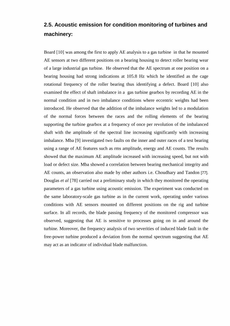
27
2.5. Acoustic emission for condition monitoring of turbines and
machinery:
Board [10] was among the first to apply AE analysis to a gas turbine in that he mounted
AE sensors at two different positions on a bearing housing to detect roller bearing wear
of a large industrial gas turbine. He observed that the AE spectrum at one position on a
bearing housing had strong indications at 105.8 Hz which he identified as the cage
rotational frequency of the roller bearing thus identifying a defect. Board [10] also
examined the effect of shaft imbalance in a gas turbine gearbox by recording AE in the
normal condition and in two imbalance conditions where eccentric weights had been
introduced. He observed that the addition of the imbalance weights led to a modulation
of the normal forces between the races and the rolling elements of the bearing
supporting the turbine gearbox at a frequency of once per revolution of the imbalanced
shaft with the amplitude of the spectral line increasing significantly with increasing
imbalance. Mba [9] investigated two faults on the inner and outer races of a test bearing
using a range of AE features such as rms amplitude, energy and AE counts. The results
showed that the maximum AE amplitude increased with increasing speed, but not with
load or defect size. Mba showed a correlation between bearing mechanical integrity and
AE counts, an observation also made by other authors i.e. Choudhary and Tandon [77].
Douglas et al [78] carried out a preliminary study in which they monitored the operating
parameters of a gas turbine using acoustic emission. The experiment was conducted on
the same laboratory-scale gas turbine as in the current work, operating under various
conditions with AE sensors mounted on different positions on the rig and turbine
surface. In all records, the blade passing frequency of the monitored compressor was
observed, suggesting that AE is sensitive to processes going on in and around the
turbine. Moreover, the frequency analysis of two severities of induced blade fault in the
free-power turbine produced a deviation from the normal spectrum suggesting that AE
may act as an indicator of individual blade malfunction.

28
Figure 2. 7: Example of AE energy of simulated damage to blades of free-power turbine (from Douglas et al[78]).
Sato [11] was also interested in applying AE to rotating machines to detect rubbing and
other damage in bearings. He mounted AE sensors on two turbine journal bearing
housings in order to detect metal wipes and bearing tilts, and found a correlation
between the AE pulse shapes and the corresponding deformation. Hall and Mba [79]
applied acoustic emission to diagnose continuous rotor-stator rubbing on a 500 MW
steam turbine operating at full load. They attached AE sensors to two different locations
on the bearing and calculated the energy envelope by applying a low order smoothing
filter to the RMS data. They found a significant amplitude difference in the AE activity
at one position over the other and attributed a modulation of the AE to fluctuations in
the rubbing force in response to the shaft whirl orbit. They attributed the higher AE
activity at one sensor to the location of the continuous rubbing being extremely close to
the sensor, and suggested that it was within 1 m of the bearing. Hall and Mba also
studied the transmission of AE waves across such very large-scale turbine rotors [12]
and found that it was possible to detect AE sources up to 2 m from the sensor and
suggested that the AE technique could be viable for detecting seal and blade rubbing in
such machines. Zuluago-Giralda and Mba [80] further investigated shaft-seal rubbing in
a 500 MW steam turbine by monitoring the AE activity during run-up and run-down,
again placing sensors at two different positions on the journal bearing case. They
measured turbine load, turbine speed, and rms AE and concluded that the rms was

29
effective in identifying the turbine's critical speed during the run-up period, but not
during the run-down period.
Figure 2. 8: AE r.m.s. (V) activity during run-down of a 500 MW turbine (from Zuluago-Giralda and Mba [80]).
Leahy et al [81]investigated the potential capability of the acoustic emission (AE)
technology for the detection of seal-to-rotor rubbing in steam turbines. They simulated
seal-to-rotor rubbing on rotor with a 4.5 ton, 2 m long, supported at each end by a 7 in
(178 mm) hydrodynamic journal bearing. The rotor and bearings were installed within a
fully enclosed test chamber with an externally mounted electric motor. Leahy et al
proved the capability of AE technique to detect simulated rubs from hydrodynamic
bearings. Armor and Frank [82] assessed AE for monitoring crack growth emission on
the rotor of a steam turbine in a noisy background environment. Attenuation studies
demonstrated the importance of having AE signals of fairly large amplitude in order that
they could be detected at the bearing position. An experiment on a laboratory test
specimen produce a large amplitude signal associated with crack growth which they
concluded would probably be detectable at full speed operation taking into account the
likely crack growth rate under various conditions.
Wang and Huang [83] used wavelet analysis in their study of AE propagation on a
Francis turbine runner to identify its attenuation characteristics. They used a standard

30
pencil lead break source and the Wavelet Packet Transform technique (WPT) for
analysis. They argued that the use of wavelet packet coefficients allowed them to reduce
the need for data storage and that the WPT is a feasible technique for monitoring the
operating turbine runners.
Many researchers have investigated AE for condition monitoring of pumps. Neill et al
[17] conducted experiments on both laboratory and industrial scale centrifugal pumps to
detect incipient cavitation. By applying both rms and frequency analysis, they were able
to detect cavitation earlier than its appearance on the pump's dynamic head and proved
the feasibility of incipient cavitation detection using AE in the face of noise from
normal running although they did suggest that the nearer the sensor is to the cavitation
site the better. Neill et al [13] extended their investigation on the AE monitoring of
pumps to their rolling bearings, comparing AE-based diagnosis with acceleration
monitoring, and concluding that AE rms and characteristics of the demodulation
frequency of resonance are good indicators of bearing defects. On the other hand, the
acceleration spectra showed a drawback, in that other peaks are present in the spectrum
associated with whole body movements of the pump to which AE is not susceptible.
Tomaž et al [84], working with 2-blade Kaplan turbine model, compared AE and video
records in order to explain the relationship between the AE and the visual appearance of
cavitation. By running at the minimum operating head with full turbine discharge,
Tomaž et al initiated the most severe cavitation conditions and concluded that there was
a correlation between the AE maximum amplitude and the cavitation number. They
found variations in the strength of the acoustic emission as the location of the cavitation
on the turbine blades moved around.
AE application to the condition monitoring of diesel engines has attracted much
attention due to the potentially high signal to noise ratio which limits the low frequency
background noise. This immunity to vibration noise is associated with the high
frequency (0.1-1.2 MHz) of AE waves so that they can act like a carrier wave [8],
allowing lower frequency information to be extracted from a signal envelope. This has
led to successful demonstrations of AE in diagnosing many engine faults such as head
gasket leaks [16], injector faults [85], combustion faults [86], and liner scuffing [87],
and the development of new processing concepts, such as engine mapping in terms of
AE events and spatially-located time-series [88, 89]. Gill et al [86] have investigated the
fuel delivery process in a four-stroke, high speed direct injection (HSDI) diesel engine

31
with two induced fault conditions. They concluded that the timing of the increase of fuel
line pressure and the time at which the injector needle becomes fully open could be
detected using AE and these times advanced while injector discharge pressure reduced.
Shuster et al [87] carried out an experimental study of piston-ring/cylinder-liner
scuffing using AE. The overall results indicated that the detected rms AE signal
provided the basis for monitoring the scuffing phenomenon dividing it into three
different levels; scuffing initiation, irreversible scuffing and severe scuffing. In
particular, the rms AE signal was sensitive to scuffing initiation through its sensitivity
to friction coefficient and it was shown that the first peak of spikes in the rms AE signal
was associated with the initial iron particles transferring from cylinder liner to piston
ring surfaces, confirmed using scanning electron microscopy (SEM). Douglas et al [90,
91] have investigated piston ring/cylinder liner interaction on a large two-stroke, slow
speed, marine diesel engine under normal operation using AE. The results showed that
it was possible to detect sliding contact between the piston rings and the cylinder liner
relating them to blow-by or exhaust valve leakage during the compression and
expansion strokes. Nivesrangsan et al [38, 39, 88, 89] conducted a thorough investigation
of the mapping of AE events generated within the cylinder head of a small HSDI diesel
engine. In doing so they introduced techniques for the spatial reconstitution [39] and source
location [88] of events using multi-sensor arrays. Good results were reported from the
reconstitution process, thereby offering more accurate information regarding event timing
and amplitude that could be used as the basis of a diagnostic system.
2.6. Artificial neural networks in condition monitoring:
This section describes how ANNs have been used in the enhancement of gas turbine
condition monitoring to show how combining ANNs with AE might be used for
recognizing the complex patterns of sensor information generated by a gas turbine.
Stephen et al [92] employed an ANN system to detect, isolate and assess faults in some
of the components of a single spool gas turbine. The ANN was combined with a
hierarchical diagnostic methodology and was tested on new data which had not been
used for training. They used six measured parameters (shaft speed, fuel flow, total gas
pressure and the temperatures of the exhaust and the compressor) of a two-shaft aero-
derivative gas turbine with the turbine power as an input to the ANN taking into
consideration the deviations of each parameter. They used a probabilistic neural

32
network (PNN) with an equal number of neurons in the input and output layers. They
found that the ANN gave more accurate fault detection compared with other diagnostic
techniques such as LGPA and NLGPA using the same input data. Fast et al [93, 94]
used an ANN for condition monitoring and fault diagnosis of a gas turbine in a
combined heat and power plant. The plant comprised a Siemens SGT800 gas turbine
with a heat recovery steam generator as well as a bio-fueled boiler and its steam cycle.
The artificial neural network models were trained with three months’ operating data
from the components of the plant. A type of multi-layer feed-forward network, the
multi-layer perceptron (MLP), was used consisting of an input layer, one hidden layer
and an output layer. The input parameters were the operating mode and the ambient
conditions, and the output parameters were the most easily measured features of the
turbine such as the output power, compressor pressure, bleed temperature, fuel flow,
and exhaust gas flow and temperature. The predicted performance from the ANN model
was tested against a number of unseen data patterns to determine the prediction error.
The accuracy of ANN modeling of the gas turbine was found to be better with proper
training and parameter selection and the study led to a functioning on-line condition
monitoring system. Junxia el al [95] used a NARMAX time series model, for a gas
turbine and analyzed it using the ANN to improve the control of the turbine. The
existing PID controller was incapable of managing the whole operating range of the
turbine and could not provide a satisfactory response to rapid changes in the dynamic
behavior due to the nonlinearities of the engine. A predictive control system using a
NARMAX model with a neural network was found to improve the PID and make it
capable of representing the engine dynamic throughout its whole operating range. The
model was tested in normal and disturbed conditions and continued to show good
control performance.
ANNs have also been used to elucidate complex patterns in AE data. . Wilkinson et al
[18], employed a back-propagation neural network for cutting tool wear prediction
using five AE features as input to classify the wear state as light, medium or heavy. The
results showed that the ANN could recognize the heavily worn tool state whenever it
occurred. The network occasionally misclassified the other states, although it always
gave a more pessimistic estimation of tool wear than was actually the case. Grabec et al
[96] used an ANN for the purposes of identifying the location of continuous AE in one
dimension (zone location). An initial set of experiments was used for the learning mode
and it contained information from two AE sensors with their coordinates relative to the

33
source as training data. The cross-correlation function of the signals from the two AE
sensors was supplied to the network to train it to the source coordinates. Application of
the trained network to new data showed that the technique was able to estimate the zone
from which the AE signals are coming.
2.7. Gas turbine faults: Gas turbines contain thousands of moving and stationary components, the most critical
of which are found in the hot environment inside the turbine where they experience high
temperatures and pressures, and high, varying stresses resulting from centrifugal loads
and aerodynamic forces. Such severe conditions provide some of the biggest challenges
in modern materials development and component design. Within the timescale of
commissioning to overhaul a number of kinds of faults can develop, including;
compressor fouling, blade erosion, blade fatigue, blade creep, corrosion, and seal
rubbing.
Compressor fouling [97, 98] is caused by the adhesion of particles bound by oil or water
mists to aerofoil and annulus surfaces. The result is an accretion that causes increased
surface roughness and, to some degree, changes the shape of the aerofoil or channel and
is most commonly encountered in gas turbine compressors. The effect of increased
roughness is to increase friction losses although changes of shape can cause more
serious operation inefficiencies.
Blade erosion [99, 100] is the abrasive removal of material from the flow path by hard
particles impinging on flow surfaces. Solid particle ingestion can be caused by a
number of mechanisms, such as vortices generated during landing and take-off, sand
storms, volcanic ash, and thrust reverser efflux at low speed which can blow ice and
dust into the engine. Erosion damage on turbine blades can be manifested as pitting and
chipping of the blade leading and trailing edges and an increase in the blade surface
roughness. The overall effects of this erosion are to increase the pressure loss and
change the blade geometry. The figure 2.9 shows the aerodynamic zones on a gas
turbine blade and identifies the severity of wear per zone.

34
Figure 2. 9: Boundary layer replica of a gas turbine blade.
Any gas turbine engine needs huge amounts of air throughout its operation, which is
provided either by sucking it in through the compressor or by ramming due to the
forward motion of an aircraft, or both. Foreign object damage (FOD) [101, 102] is
caused by debris which can either be hard objects such as stones, hardware and
pavement fragments, or soft-bodies such as ice, birds and animals. FOD is typically
caused when the rotating blade strikes an object, and the velocity of the blade is usually
more significant than the axial velocity of the object. The result of the impact is a
localized damage in the form of a notch or dent (typically on, or close to, the leading
edge). The overall result of FOD on the gas turbine is a reduction of the fine balance of
the system and degradation of the airflow characteristics over the blade aerofoil, leading
to aerodynamically-induced vibration or flutter, which initiates fatigue failures excited
at rotation or blade passing frequencies.

35
Blade fatigue failures [103, 104] are most often caused by anomalies in mechanical
behavior and/or manufacturing defects. There are two kinds of blade fatigue failure,
high cycle fatigue (HCF) and low cycle fatigue (LCF). HCF is rare in turbine blades,
unless some form of initiation damage is present, and/or there is excessive bending of
the blades for example due to abnormal vibration in the engine. HCF cracks are most
likely to be initiated at the surface in the brittle platinum aluminized coating layer and
may spend much of the fatigue life very small, accelerating in size with time due to the
stress intensification effect and propagating progressively across the thickness of the
blades. Once the fatigue crack reaches a critical length it will propagate across the
remaining section by fracture leading to other damage in the engine. LCF is related to
the much larger stress cycles imposed by starting and stopping operations and
constitute the design-limiting fatigue life cycles. The source of these stresses is fairly
apparent. When stopped, the disc/blade combination is subjected to loadings mainly
due to its self-weight, and is relatively cold. However, in operation the same
components are subject to large, though fairly constant loadings from centrifugal forces
imposed by the rotational speed, and are at a much higher temperature. The rate of
change between these two states is rapid on engine start, inducing high levels of
thermal stress, which reach a steady state during operation and then reappear, in
reverse, during cool-down. Thus, the number of fatigue cycles is relatively low,
although the stress range is high.
Fatigue cracks can appear at a number of locations on the blades, such as; on the
aerofoil above the blade root platform near the trailing edge on the concave side of the
blade (Figure 2.10, red arrow), on the aerofoil above the blade root platform near the
trailing edge on the convex side of the blade (Figure 2.10, white arrow), and on the
aerofoil of the blade just above the fillet radius from the trailing edge, Figure 2.11.
Fatigue cracks always initiate at the blade surface irrespective of location on the blade
and this is because the surface changes temperature more rapidly than the interior,
giving it the highest thermal stresses.

36
Figure 2. 10: Fracture surface of a blade with fatigue failure on the concave side near trailing edge (TE: trailing edge; LE: leading edge) [103].
Figure 2. 11: Fracture surface of a blade with fatigue failure on the convex side near trailing edge (TE: trailing edge; LE: leading edge) [103].

37
Blade creep [105, 106] manifests itself as blade ‘‘stretch’’ in which the blade elongates
plastically in service under the centrifugal loads. In abnormal conditions and severe
situations, this may be sufficient for the blade tip to contact the non-rotating shroud,
causing a ‘‘tip rub’’. Blades fail by creep when the normal operating temperatures of the
engine are exceeded for more than brief periods or when the inspection procedures are
not correctly followed.
Hot corrosion [107, 108] is the loss of material from flow path components caused by
chemical reactions between the component and certain contaminants, such as Na2SO4,
NaCl, and V2O5 that combine to form molten deposits, which damage the protective
surface oxides. There are two kinds of hot corrosion, high temperature hot corrosion
(HTHC) and low temperature hot corrosion (LTHC).
HTHC is observed mainly within the temperature range of 850 to 950°C and starts with
the condensation of alkali metal salts on the surface of the component. The dominant
salt in HTHC is Na2SO4 due to its high thermodynamic stability. HTHC can be divided
into four progressive stages from initial onset to failure. In stage 1, slight roughening of
the surface caused by some growth and localized breakdown of the oxide scale layer is
evident. At this stage, neither chromium depletion in the substrate layer nor loss of
mechanical integrity is observed. In stage 2, the roughness of the surface is more
marked as the oxide layer breakdown continues. While chromium depletion
commences at this stage, mechanical integrity is still not affected. In stage 3, oxidation
of the base material has penetrated to a significant depth, with an obvious build-up of
scale. At this stage, the mechanical integrity has been compromised and the blades are
normally removed from service. Progression to stage 4 (catastrophic attack) will occur
with or without the continued presence of sodium. In stage 4, the attack penetrates
deeply into the blade while forming a large `blister' of scale, and failure is likely to
occur due to loss of structural integrity.
LTHC is observed mainly within the temperature range of 650 to 800°C. LTHC
produces a characteristic type of pitting, resulting from the formation of low melting
temperature (eutectic) mixtures of Na2SO4 and CoSO4. The initiation of LTHC is often
attributed to failure of the protective oxide layer, which allows the molten salt direct
access to the substrate metal. Ultimate failure may result from enhanced erosion,

38
thermal stresses, erosion-corrosion, and/or chemical reactions. LTHC develops in two
stages, the formation of liquid sodium-cobalt sulphate on the surface and the
propagation of attack via migration of SO3 and cobalt inward and outward,
respectively, through the liquid salt.
Hot corrosion is usually greatest at the hottest point on the pressure (concave) surface
of the turbine blades about midway along the length of the blade, and a short distance
back from the leading edge. It is more frequently observed in the low-pressure turbine
(LPT) than in the high pressure turbine (HPT) due to the lower temperatures involved
in the LPT where the corrosive contaminants are more likely to accumulate on the
surface in significant amounts and/or for a greater percentage of time.
Seal rubbing [109, 110] can occur between the static and rotating components of the
turbine. Rubbing in the seal is a secondary phenomenon which results from a primary
cause such as high lateral rotor vibrations and high lateral displacement of the rotor
centre line due to misalignment. There are two main types of rubbing. The first type is
“light partial rubbing” where the contact forces are minimal, and the rotating elements
occasionally touch the stationary elements. The second type “continuous rubbing” is
more serious because of its influence on the integrity of the machine. This is a full
annular rub in which the rotor maintains contact with the seal continuously or almost
continuously. Seal rubbing must be avoided as it will ultimately result in wear and an
increased leakage flow between the high-pressure and the low-pressure sections which
will reduce the efficiency of the gas turbine leading to eventual shut down.
Many of these faults are associated with mechanisms of failure which will generate AE.
Some faults produce AE directly such as contact between rotor and stator, damage in
bearings, and rotor crack propagation. Other faults such as: abnormal dynamic loading;
wear, accretion or corrosion of flow surfaces; misalignment, lubrication degradation, oil
starvation, and foreign object damage produce AE indirectly. AE has been found to
offer better performance than some other techniques for detecting faults in turbines such
as rubbing [12, 79, 111], and damage in bearings [9, 112-114]. For example, vibration
monitoring of the bearing pedestals has been studied using accelerometers to identify
shaft seal rubbing in turbines and found not to be as effective as AE [115, 116] which
can detect faults in the early stages of the rotor-stator rubbing. The high amplitude, high
frequency (20KHz-2MHz) AE signatures associated with rubbing [117] can propagate

39
across the turbine for distances of up to 4 meters, allowing the AE technique to identify
the onset and the location of the rubbing in the turbine. However, this success is
considered to be dependent on fully understanding the background noise received by the
sensor on an operational turbine unit.
2.8. Summary of state of knowledge and thesis identification:
Established condition monitoring techniques for gas turbines such as gas path analysis,
oil analysis, and vibration analysis use such parameters as temperature, pressure, speed,
accelerometer signals, and oil features to identify the machine condition and to achieve
economic performance through increased availability and reduced component
replacement costs. However, those techniques are all indirect; they do not provide
enough information about degradation in gas turbines at the early stages of fault
development and many of them have limited, or no, capacity to locate the sources of
faults. The acoustic emission technique addresses these drawbacks by its capability to
monitor degradation processes as well as their symptoms inferring an ability to identify
changes in the early stages, as well as the capacity to locate the source of any non-
continuous AE.
However, the high temperatures in the gas flow areas of gas turbines and the low signal-
to-noise ratio has limited the application of AE on industrial machines to studies of
bearing defects, rubbing damage, background noise determination and AE propagation
characteristics on off-service engines.
A number of the faults that can occur in turbines result in changes to the gas flow over
the various operating surfaces and it were decided to address this area of turbine
monitoring, as little or no work has been done on this aspect. It was expected that a
breakthrough in the application of AE to gas turbines could be achieved by a full
understanding of what influences the AE behavior emanating from a gas turbine at
various running conditions and differentiating between AE sources resulting from gas
flow through the turbine and those resulting from impact or rolling contact in the
ancillary mechanical equipment, such as shafts and bearings. This work, therefore,
concentrates on establishing the AE signatures of a laboratory-scale gas turbine under
normal running conditions and with faults induced in the flow behavior through the free
power turbine, by jamming its impeller, removing its power take-off, introducing
defects in its blades, and removing the impeller entirely.

40
Chapter 3 Experimental apparatus and procedures
3.1. Introduction:
This chapter is divided into two parts the first part describes all the requirements and
specifications of the apparatus used, and the second part explains all the procedures and
arrangements for the research experiments, including calibration. The second part is divided
into three sections, the first of which describes the calibration of the AE sensors using
simulated sources on a steel block and on the turbine rig and including AE propagation tests
on the turbine rig, The second section explains the procedure for the experiments carried out
on the turbine under normal running conditions, with the impeller jammed, with the
impeller absent, with load and without load. The final section describes the procedure for
investigating the effect of impeller damage.
3.2. Apparatus: A typical AE acquisition system and experimental set-up as used in this work are shown
schematically in Figure 3.1. The system generally comprises a test object (here shown as
the turbine), an array of AE sensors with their associated pre-amplifiers, a data acquisition
card, and a computer with software for controlling the acquisition and storage of data.
Figure 3.1: Schematic view of turbine rig and acoustic emission system.
The following sub-sections describe each of these component parts of the set-up.

41
3.2.1. AE sensors and coupling: Two types of AE sensors were used in this work. The first type is a commercial
broadband AE sensor of type Micro-80D (Physical Acoustics, PAC), shown in Figure
3.2, chosen for its versatility and wide use for machinery monitoring tests. The sensor
based on lead zirconate titanate (PZT), is omni-directional and produces a relatively flat
but resonant frequency response from 175-1000 kHz, over an operating temperature
range from 65- to 177+ 0C [118]. The sensor is 10 mm in diameter and 12 mm high
and was held onto the test object surface using an in-house designed magnetic clamp. In
order to obtain good transmission of the AE from the test object to the sensor, the
surface was kept smooth and clean and silicone grease was used as couplant to fill any
gaps caused by surface roughness and to eliminate any air gaps which might otherwise
impair AE transmission. The sensitivity of the sensor at each position was checked
using a simulated source by breaking a pencil lead close to it, against expected signal
amplitude of around 4-5 volts using the fixed amplifier settings.
Figure 3.2: Micro-80D broad band sensor.
The second AE sensor used was of type S9215, also from PAC and is specially
designed for high temperature operation. This AE sensor, shown in Figure 3.3 is also
omnidirectional and produces a resonant response from 65050 - kHz; over an
operating temperature range from 200- to 540+ Co . The sensor is 20 mm in diameter
and 20 mm high. The lower frequency resonant response required the use of a
preamplifier with a lower high-pass filter, passing frequencies above 20 kHz [119]. This
kind of sensor offers a good opportunity to acquire AE from positions on hot surfaces
close to the likely sources of AE but the lower frequency response causes difficulties
with increased noise levels and the possibility that some aspects of the signal will not be
captured. The S9215 sensor is used in high temperature nuclear and fossil fuel utility

42
plants, to monitor leaks and cracks in pipelines and vessels, and in aerospace engine
monitoring applications. A high-temperature grease (UCA-HT from Ely chemical) was
used as couplant for this sensor.
Figure 3.3: S9215 narrow band, high temperature sensor[119].
3.2.2. Preamplifiers:
The preamplifier (type PAC 1220A) shown in Figure 3.4 was used to amplify the AE
signal from the Micro-80D sensor to a level that can be comfortably transmitted and
converted by an Analogue to Digital Converter (ADC). These amplifiers have internal
band pass filters from 0.1-1.2 MHz and a switchable gain between 40 and 60 dB. The
preamplifier is powered by a 28+ V power supply and used a single BNC connection
for both power and signal.
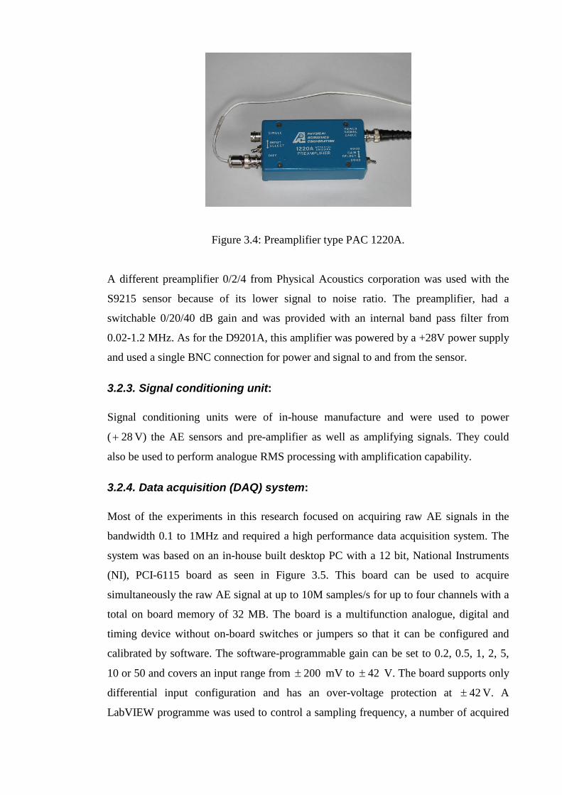
43
Figure 3.4: Preamplifier type PAC 1220A. A different preamplifier 0/2/4 from Physical Acoustics corporation was used with the
S9215 sensor because of its lower signal to noise ratio. The preamplifier, had a
switchable 0/20/40 dB gain and was provided with an internal band pass filter from
0.02-1.2 MHz. As for the D9201A, this amplifier was powered by a +28V power supply
and used a single BNC connection for power and signal to and from the sensor.
3.2.3. Signal conditioning unit: Signal conditioning units were of in-house manufacture and were used to power
( 28+ V) the AE sensors and pre-amplifier as well as amplifying signals. They could
also be used to perform analogue RMS processing with amplification capability.
3.2.4. Data acquisition (DAQ) system: Most of the experiments in this research focused on acquiring raw AE signals in the
bandwidth 0.1 to 1MHz and required a high performance data acquisition system. The
system was based on an in-house built desktop PC with a 12 bit, National Instruments
(NI), PCI-6115 board as seen in Figure 3.5. This board can be used to acquire
simultaneously the raw AE signal at up to 10M samples/s for up to four channels with a
total on board memory of 32 MB. The board is a multifunction analogue, digital and
timing device without on-board switches or jumpers so that it can be configured and
calibrated by software. The software-programmable gain can be set to 0.2, 0.5, 1, 2, 5,
10 or 50 and covers an input range from 200± mV to 42± V. The board supports only
differential input configuration and has an over-voltage protection at 42± V. A
LabVIEW programme was used to control a sampling frequency, a number of acquired
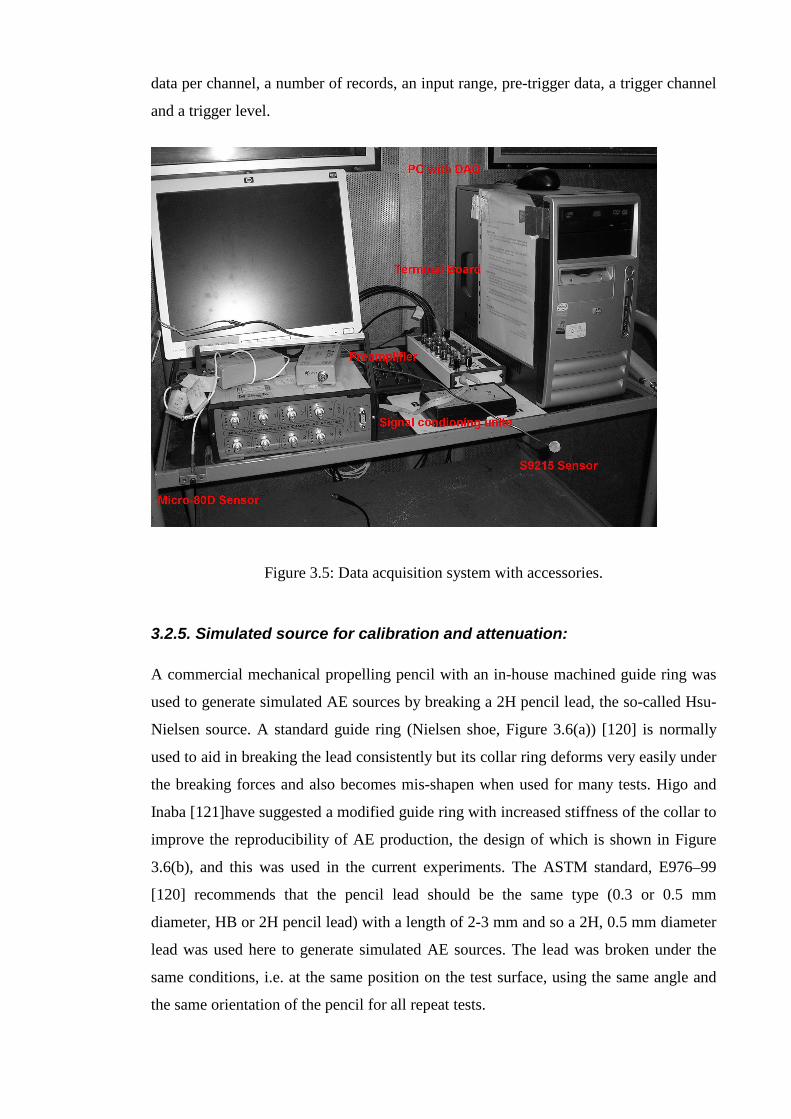
44
data per channel, a number of records, an input range, pre-trigger data, a trigger channel
and a trigger level.
Figure 3.5: Data acquisition system with accessories.
3.2.5. Simulated source for calibration and attenuation: A commercial mechanical propelling pencil with an in-house machined guide ring was
used to generate simulated AE sources by breaking a 2H pencil lead, the so-called Hsu-
Nielsen source. A standard guide ring (Nielsen shoe, Figure 3.6(a)) [120] is normally
used to aid in breaking the lead consistently but its collar ring deforms very easily under
the breaking forces and also becomes mis-shapen when used for many tests. Higo and
Inaba [121]have suggested a modified guide ring with increased stiffness of the collar to
improve the reproducibility of AE production, the design of which is shown in Figure
3.6(b), and this was used in the current experiments. The ASTM standard, E976–99
[120] recommends that the pencil lead should be the same type (0.3 or 0.5 mm
diameter, HB or 2H pencil lead) with a length of 2-3 mm and so a 2H, 0.5 mm diameter
lead was used here to generate simulated AE sources. The lead was broken under the
same conditions, i.e. at the same position on the test surface, using the same angle and
the same orientation of the pencil for all repeat tests.
45
Ø GT
Ø 2.0
Ø 7.0
0.5
Ø 7.0
0.5
Ø 2.0
Ø GT
Mechanical pencil
Teflon guide ring
Guide tube
2H, Ø 5 mm.Pencil lead
Mechanical pencil
Guide tube
Teflon guide ring
Pencil lead2H, Ø 5 mm.
Diameter GT (± 0.05 mm)0.3 mm0.5 mm
0.84 mm0.92 mm
GUIDE RINGTEFLONDIMENSIONS GIVEN IN mm.TOLERENCE ± 0.1 mm.
(a) Standard guide ring (Nielsen shoe)
(b) Modified guide ring
References:1. ASTM Standards E 976 - 992. Higo, Y. and Indba, H., ASTM STP 1077, 1991.
Figure 3.6: Drawings and dimensions of standard (a) and modified (b) guide rings[120, 121] .
3.2.6. Gas Turbine Rig:
The gas turbine used was a P.9000 gas turbine [122] unit manufactured by Cussons
Ltd., shown schematically in Figure 3.7. The gas turbine consists of two stages. The
first stage is gas generator which is a compressor and turbine mounted back to back on a
short shaft supported in a journal bearing. The second stage is the free power turbine
which is a single stage radial turbine operating over the range 170 to 600 rps and
developing a maximum power of approximately 4 kW. The free power turbine is
connected with an alternator which generates electricity that could be dissipated through
heat lamps or made available from normal plug sockets. The change in the excitation
voltage applied to the alternator field coils allows the power loading on the alternator
(and hence the turbine) to be easily variable over the required operating range. The
efficiency of the converted power between free power turbine and alternator could reach
85%.
The turbine was fuelled by propane, delivered from standard gas take-off bottles.
Consumption was approximately 3.2 g/s at full load and about 1.1 g/s idling with no
loading. Cooling was via an oil/water heat exchanger at about 10 liters per minute and
the oil temperature was automatically controlled by a thermostat and solenoid valve
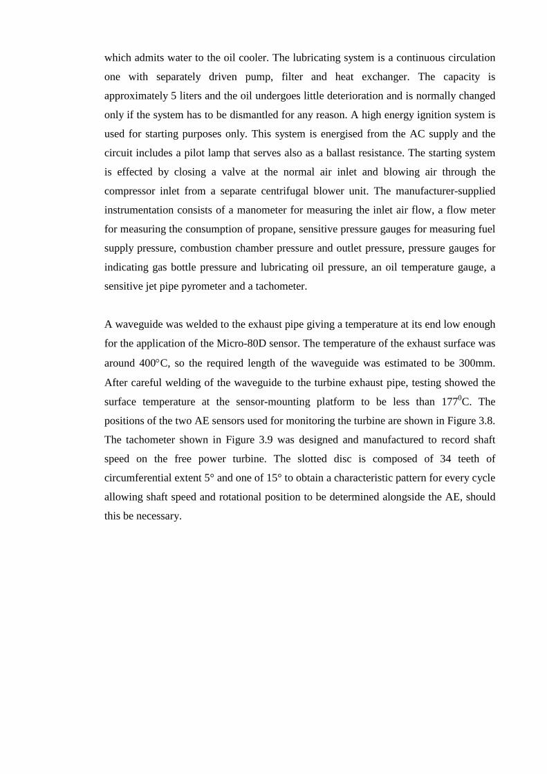
46
which admits water to the oil cooler. The lubricating system is a continuous circulation
one with separately driven pump, filter and heat exchanger. The capacity is
approximately 5 liters and the oil undergoes little deterioration and is normally changed
only if the system has to be dismantled for any reason. A high energy ignition system is
used for starting purposes only. This system is energised from the AC supply and the
circuit includes a pilot lamp that serves also as a ballast resistance. The starting system
is effected by closing a valve at the normal air inlet and blowing air through the
compressor inlet from a separate centrifugal blower unit. The manufacturer-supplied
instrumentation consists of a manometer for measuring the inlet air flow, a flow meter
for measuring the consumption of propane, sensitive pressure gauges for measuring fuel
supply pressure, combustion chamber pressure and outlet pressure, pressure gauges for
indicating gas bottle pressure and lubricating oil pressure, an oil temperature gauge, a
sensitive jet pipe pyrometer and a tachometer.
A waveguide was welded to the exhaust pipe giving a temperature at its end low enough
for the application of the Micro-80D sensor. The temperature of the exhaust surface was
around 400°C, so the required length of the waveguide was estimated to be 300mm.
After careful welding of the waveguide to the turbine exhaust pipe, testing showed the
surface temperature at the sensor-mounting platform to be less than 1770C. The
positions of the two AE sensors used for monitoring the turbine are shown in Figure 3.8.
The tachometer shown in Figure 3.9 was designed and manufactured to record shaft
speed on the free power turbine. The slotted disc is composed of 34 teeth of
circumferential extent 5° and one of 15° to obtain a characteristic pattern for every cycle
allowing shaft speed and rotational position to be determined alongside the AE, should
this be necessary.

47
Figure 3.7: Schematic diagram of turbine rig showing positions of temperature and pressure sensors.
Figure 3.8: Photograph of turbine rig showing AE sensor positions.

48
Figure 3.9: Timing signal system
3.3. Experimental procedure: Three types of experiments were done; tests with the turbine running normally with and
without power being taken off, tests with the impeller jammed and absent and, finally,
tests with simulated blade defects. The rationale behind these experiments is described
below. Essentially, the objective was first to determine what the sources of AE are in a
turbine and then to determine whether these sources might give useful diagnostic
information under normal operating conditions and/or fault conditions.
3.3.1. Turbine running tests:
The purpose of this set of tests was to find the AE characteristics associated with the
processes going on in the running turbine. To do this, the two calibrated sensors and
positions were used, and the turbine run in a variety of conditions including normal
running with and without load, and in two conditions where the behavior was simplified
by jamming the impeller so that it did not rotate and with the impeller removed from the
free power turbine. The turbine shaft speed of the gas generator was varied between
30000 and 70000 rpm which, accordingly, changes the free power turbine speed (if the
impeller is operating normally). Figure 3.10 shows the general arrangement for the
turbine running tests.

49
Figure 3.10: Running test arrangement showing free power turbine with AE sensors and
power take-off belt.
3.3.1.1. Turbine running test with jammed impeller and without impeller:
For this experiment, the impeller of the free power turbine was either jammed by
connecting the turbine belt to a fully loaded alternator, or entirely removed from the
turbine. When the impeller was removed, it was necessary to replace it with a dummy
piece (Figure 3.11) which allowed free passage of gas through the shroud but prevented
gas leakage from the free power turbine to the lubrication system. Three, nominally
identical tests were run for each of the jammed impeller and absent impeller
configurations. Each test consisted of acquiring data over a range of incrementally
increased gas generator shaft speeds between 500-1150 RPS achieved by means of
changing the fuel flow. At each operating condition, fuel flow, air flow, and gas
pressure and temperature of both the compressor and turbine were recorded as these
were not precisely reproducible between tests. At each operating condition, raw AE was
recorded for 0.03 sec and 20 records were obtained at each operating condition.

50
Figure 3.11: Schematic of dummy piece used to replace the impeller.
3.3.1.2. Turbine normal running test with and without load:
In this series of experiments, AE was acquired over a range of free power turbine speeds
while the machine was under load and not under load. For the loaded condition, the
speed of the gas generator was kept constant, and the speed change in the free power
turbine was achieved by changing the alternator load. For the no-load (idling) condition,
the connecting belt between the free power turbine and the alternator was removed and
the turbine speed changed by changing the fuel flow incrementally which, accordingly,
resulted in changes in both the gas generator and free power turbine speeds. The speed
of the free power turbine was measured by means of the optical sensor connected to the
slotted disc at the end of free power turbine shaft, and other operating parameters such
as the gas generator speed fuel flow, air flow, and gas pressure and temperature of both
the compressor and turbine, were recorded as for the other tests.
For each of the two conditions, with and without load, the speed was varied between
120 RPS and 380 RPS and 20 records of raw AE of length 0.03 sec acquired at each
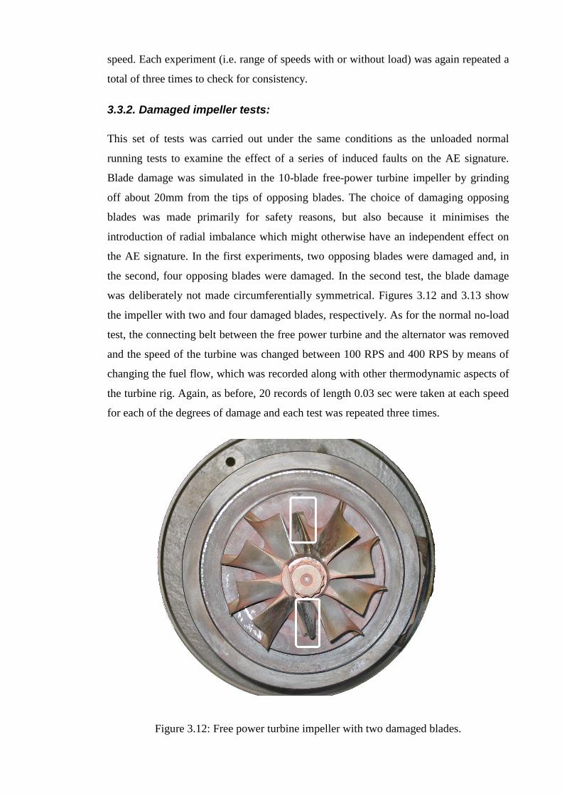
51
speed. Each experiment (i.e. range of speeds with or without load) was again repeated a
total of three times to check for consistency.
3.3.2. Damaged impeller tests: This set of tests was carried out under the same conditions as the unloaded normal
running tests to examine the effect of a series of induced faults on the AE signature.
Blade damage was simulated in the 10-blade free-power turbine impeller by grinding
off about 20mm from the tips of opposing blades. The choice of damaging opposing
blades was made primarily for safety reasons, but also because it minimises the
introduction of radial imbalance which might otherwise have an independent effect on
the AE signature. In the first experiments, two opposing blades were damaged and, in
the second, four opposing blades were damaged. In the second test, the blade damage
was deliberately not made circumferentially symmetrical. Figures 3.12 and 3.13 show
the impeller with two and four damaged blades, respectively. As for the normal no-load
test, the connecting belt between the free power turbine and the alternator was removed
and the speed of the turbine was changed between 100 RPS and 400 RPS by means of
changing the fuel flow, which was recorded along with other thermodynamic aspects of
the turbine rig. Again, as before, 20 records of length 0.03 sec were taken at each speed
for each of the degrees of damage and each test was repeated three times.
Figure 3.12: Free power turbine impeller with two damaged blades.

52
Figure 3.13: Free power turbine impeller with four damaged blades.
3.4. AE transmission and calibration tests: Before carrying out any experiments, it was first necessary to calibrate the AE sensors
and assess the transmission between various parts of the turbine and the sensor
positions. Calibration tests were carried out on a steel block and on the turbine in order
to check the response of the AE sensors and note any changes with temperature or time.
It was also necessary to check the degree of reproducibility that could be expected after
removing and replacing a sensor (i.e. the reproducibility of coupling). Finally, it was
also necessary to know the relative sensitivity of the two different sensors used.
The transmission experiments were carried out to establish the characteristics of AE
wave propagation through and over the surface of the gas turbine, including the
waveguide. Attenuation of AE energy and changes to frequency content were measured
for a variety of sensor source positions.
All calibration and transmission experiments used a pencil lead break as the AE source and
AE energy as the main quantitative feature of the signal. All lead breaks were recorded at
5MHz for duration of 0.015 sec.

53
3.4.1. Calibration tests on steel block: A large cylindrical steel block of dimensions 307mm diameter and 166mm height was
used to calibrate sensors back-to-back. Pencil leads were broken on the centre of the top
surface of the block typically with an array of three AE sensors mounted at the same
radial distance, 62.5 mm from the source (Figure 3.14). The aims of this calibration
were: to provide a means of calibrating the sensors before and after each test, to assess
the variation of recorded AE due to individual pencil lead breaks and with individual
installations (effect of coupling variation), and to compare the sensitivity and frequency
response of the two types of sensors used. To investigate these effects, three Micro80D
sensors were used at four sensor positions separated circumferentially by 90°. With the
three sensors in each position 10 pencil lead breaks were recorded and the sensors
removed and replaced in the same positions and another 10 breaks recorded. This
process was repeated for a total of ten times so that 100 breaks were recorded for each
sensor at each position. Next, the sensors were moved to another position and the entire
process repeated.
Figure 3.14: (a) Overall schematic and (b) plan view of sensor positions on steel calibration block.
(a) (b)

54
Figure 3.15 summarises the recorded AE energy for the pencil lead breaks for all
sensors at all positions. The wave arrival was identified by the time at which the signal
level first exceeds a threshold of 1.5 times the maximum amplitude of the noise
recorded in the first 180 µs. The energy was calculated by integrating the square of the
amplitude for the duration between the first and the last threshold crossing. It is clear
from Figure 3.15 that there is some variation between sensors and positions, but also
that there is considerable variation for a given sensor in a given position. In order to
analyse the data more systematically, a single factor analysis of variance was carried out
grouping the data in a range of ways.
Figure 3.16 shows sensor 1 energy distribution at the four positions and the 10 removal-
replacements at each position. Grouping the individual placements at a given position,
the variance between placements (variation in coupling) can be compared with the
variance within a given placement (variation in pencil lead breaks). The indicator Fvalue
is compared with Fcrit (1.98 for the degrees of freedom involved and at the 95%
confidence level) and, as can be seen in Figure 3.16, Fvalue is always greater than Fcrit
indicating that the effect of removal and replacement of the sensor is more important
than the variation in pencil lead breaks at all positions. Table 3.1 shows the value of
Fvalue for all sensors at all positions and, confirming the same findings for all sensors.
0
0.5
1
1.5
2
2.5x 10
-6
E(V
2 .S)
P2 P2
Sensor1 Sensor3Sensor2
P1 P3 P4 P1 P2 P3 P1 P3P4 P4
Figure 3.15: AE energy recorded at the three sensors on the steel block at four positions.

55
0 1 2 3 4 5 6 7 8 9 10 110
1
2x 10
-6 (a)
Replace number
E(V
2.S
)
0 1 2 3 4 5 6 7 8 9 10 110
1
2x 10
-6 (b)
Replace number
E(V
2.S
)
0 1 2 3 4 5 6 7 8 9 10 110
1
2x 10
-6 (c)
Replace number
E(V
2.S
)
0 1 2 3 4 5 6 7 8 9 10 110
0.5
1x 10
-6 (d)
Replace number
E(V
2.S
)
F>Fcrit12.9>1.98
F<Fcrit1.99>1.98
F>Fcrit8.3>1.98
F>Fcrit5.5>1.98
Figure 3.16: Sensor 1 energy distribution for 10 placements at four positions; (a)
position 1, (b) position 2, (c) position 3, (d) position 4.
Sensor Position F Value
1 1 12.9696 1 2 1.9978 1 3 8.3188 1 4 5.5898 2 1 8.5964 2 2 2.3407 2 3 13.9594 2 4 3.4022 3 1 2.8630 3 2 1.9942 3 3 11.2764 3 4 17.6060
Table 3.1: Summary of Anova results comparing effects of variation in source with variation in coupling for each sensor at each position.

56
The data for each position for all three sensors has been grouped to analyse the variance
between positions and within positions. This will compare the effect of position with the
effect of lead break, sensor and coupling. Table 3.2 shows that Fvalue is always greater
than Fcrit (3.026 for the degrees of freedom involved and at the 95% confidence level)
which indicates that the effect of changing position is more important than the variation
in pencil lead breaks, sensor and coupling. Finally the data for each sensor at all four
position has been grouped to analyse the variance between sensors with variance from
lead break, position and coupling. The Fvalue is again greater than Fcrit which indicates
that the effect of changing sensor is significant and led to the use of the same sensor for
all experiments.
Position F Value 1 27.9 2 140.2 3 14.6 4 131.8
Table 3.2: Summary of Anova results comparing effects of variation in position with variation in lead break, sensor and coupling at each position.
Next, the S9215 sensor and the selected Micro-80D sensor were calibrated back-to-back
on the steel block. The two sensors were mounted at the same radial distance, 62.5 mm
from the source, and 100 pencil lead breaks acquired without moving or removing
either sensor. The objective of this calibration was to identify the variation in sensitivity
between sensors. The average AE energy of both sensors was calculated using equation
2.4 and it was found that the Micro-80D sensor gave AE energy 80-140 times higher
than the S9215 sensor using the same gain settings as in the experiment. Figure 3.17
shows the raw AE spectra for both sensors on steel block, reflecting the narrow
bandwidth of the S9215 sensor (50-250 kHz) compared with the Micro-80D sensor
(100-400 kHz). Appendix A contains sensitivity calibration certificates for AE
transducers S9215, and Micro-80D.
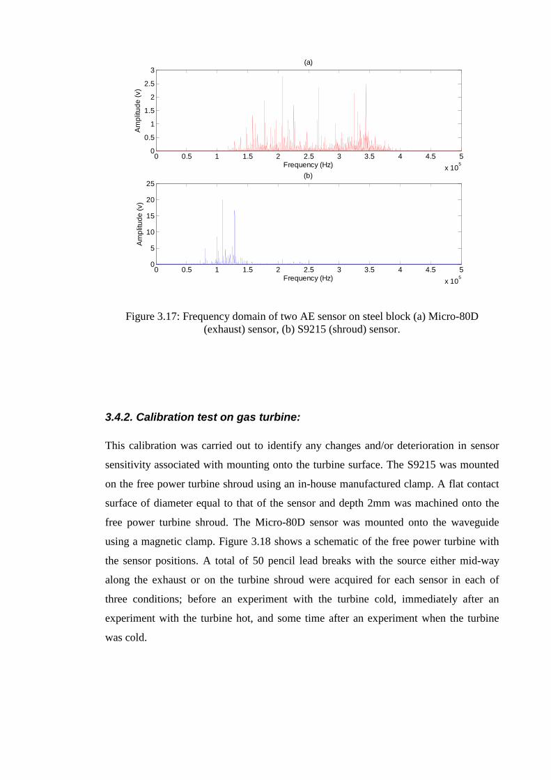
57
0 0.5 1 1.5 2 2.5 3 3.5 4 4.5 5
x 105
0
0.5
1
1.5
2
2.5
3
Frequency (Hz)
Am
plit
ud
e (
v)
(a)
0 0.5 1 1.5 2 2.5 3 3.5 4 4.5 5
x 105
0
5
10
15
20
25
Frequency (Hz)
Am
plit
ud
e (
v)
(b)
Figure 3.17: Frequency domain of two AE sensor on steel block (a) Micro-80D
(exhaust) sensor, (b) S9215 (shroud) sensor.
3.4.2. Calibration test on gas turbine: This calibration was carried out to identify any changes and/or deterioration in sensor
sensitivity associated with mounting onto the turbine surface. The S9215 was mounted
on the free power turbine shroud using an in-house manufactured clamp. A flat contact
surface of diameter equal to that of the sensor and depth 2mm was machined onto the
free power turbine shroud. The Micro-80D sensor was mounted onto the waveguide
using a magnetic clamp. Figure 3.18 shows a schematic of the free power turbine with
the sensor positions. A total of 50 pencil lead breaks with the source either mid-way
along the exhaust or on the turbine shroud were acquired for each sensor in each of
three conditions; before an experiment with the turbine cold, immediately after an
experiment with the turbine hot, and some time after an experiment when the turbine
was cold.
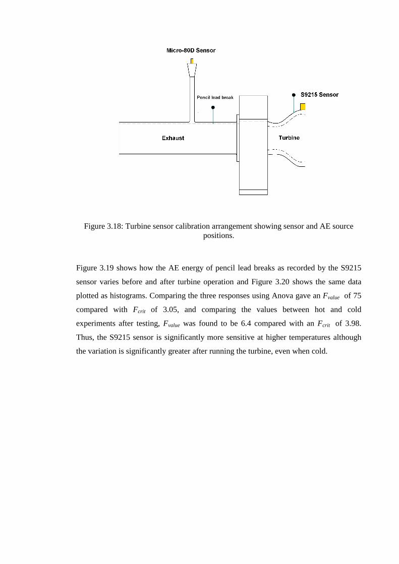
58
Figure 3.18: Turbine sensor calibration arrangement showing sensor and AE source
positions.
Figure 3.19 shows how the AE energy of pencil lead breaks as recorded by the S9215
sensor varies before and after turbine operation and Figure 3.20 shows the same data
plotted as histograms. Comparing the three responses using Anova gave an Fvalue of 75
compared with Fcrit of 3.05, and comparing the values between hot and cold
experiments after testing, Fvalue was found to be 6.4 compared with an Fcrit of 3.98.
Thus, the S9215 sensor is significantly more sensitive at higher temperatures although
the variation is significantly greater after running the turbine, even when cold.

59
1
2
3
4
5
6
7
8
9
10
11
x 10-9
E(V
2.S
)
Before turbine operationafter turbine operation(hot)After turbine operation(cold)
Figure 3.19: AE energy calibration of S9215 sensor on turbine rig.
Figure 3.20: Histogram of AE energy for S9215 sensor calibration on turbine rig, (a) before turbine operation, (b) after turbine operation (hot), (c) after turbine operation
(cold).
Figures 3.21 and 3.22 show the AE energy and histograms for the Micro-80D sensor for
the turbine calibration experiment. Carrying out Anova among the three conditions gave
a value of Fvalue of 55.3 compared with Fcrit of 3.98, and comparing the hot and cold
0 0.1 0.2 0.3 0.4 0.5 0.6 0.7 0.8 0.9
x 10
0
10
20
30(a)
E(V)
Fre
qu
en
cy
0 0.1 0.2 0.3 0.4 0.5 0.6 0.7 0.8 0.9
x 10
0
10
20
30(b)
E(V)
Fre
qu
en
cy
0 0.1 0.2 0.3 0.4 0.5 0.6 0.7 0.8 0.9
x 10
0
10
20
30(c)
E(V)
Fre
qu
en
cy

60
values before and after testing gave Fvalue of 4.58 against an Fcrit again of 3.98. Thus,
the Micro-80D sensitivity goes down when the turbine is hot, even though it should be
within its normal operating temperature range. Once the temperature returns to normal,
the response is practically the same as it was before the test.
0
0.5
1
1.5
2
2.5
3
3.5
4
4.5x 10
-7E
(V2 .S
)
Before turbine operationAfter turbine operation(hot) After turbine operation(cold)
Figure 3. 21: AE energy calibration of Micro-80D sensor on turbine rig.
0 0.5 1 1.5 2 2.5 3 3.5 4
x 10-7
0
10
20
E(V)
Fre
qu
ency
0 0.5 1 1.5 2 2.5 3 3.5 4
x 10-7
0
10
20
E(V)
Fre
qu
ency
0 0.5 1 1.5 2 2.5 3 3.5 4
x 10-7
0
10
20
E(V)
Fre
qu
ency
Figure 3. 22: Histogram of AE energy for Micro- 80D sensor calibration on turbine rig, (a) before turbine operation, (b) after turbine operation (hot), (c) after turbine operation
(cold).

61
3.4.3. AE propagation on gas turbine: These tests were carried out to investigate the attenuation and frequency distortion of
sources at various positions on the free power turbine as recorded by the two different
AE sensors at the two different positions (turbine shroud and turbine waveguide). Thus,
the effects not only of source-sensor distance, but also aspects of the geometry of the
turbine such as discontinuities, webs and non-uniform cross section could be studied for
potential sources resulting from gas flow through the turbine blades and exhaust, oil
lubrication, and bearings in addition to unwanted sources such rubbing of mountings
due to vibration. In this test three AE sensors were used, two Micro-80D sensors and
one S9215 sensor. One Micro-80D sensor was positioned on the waveguide (as used in
the experiments) and another on the turbine shroud adjacent to the S9215 sensor in
order to assess the relative effects of sensor type. The source position was moved along
the free power turbine starting at the shroud and ending at the exhaust with ten repeat
breaks being recorded for each sensor at each position. Figure 3.23 shows the sensors
and source positions.
Figure 3.23: Turbine propagation test arrangement showing sensors and AE source positions.

62
The energy, calculated as for the calibration tests, was plotted as a function of source-sensor
distances and the best-fit exponential decay curve, according to equation (2.4), used to
determine an attenuation coefficient. Figures 3.24 and 3.25 show the energy plots with the
best-fit exponential decay curves for the S9215 sensor and Micro-80D sensor, respectively,
mounted on the turbine shroud. Both figures exhibit high variability of AE energy in the
region close to the sensor position, i.e. on the turbine shroud. Such an effect has been
attributed [27, 32, 123] to the complicated near-field waves compared with reflected waves.
Both graphs also show a marked reduction in energy following major discontinuities in the
structure, illustrated as vertical dotted lines.
Figure 3.24: AE energy versus source-sensor distance with best-fit exponential decay curve for S9215 sensor mounted on turbine shroud.
-0.05 0 0.05 0.1 0.15 0.2 0.250
0.2
0.4
0.6
0.8
1
1.2
1.4
1.6
1.8
x 10-10
Source-Sensor Distance(m)
E(v
2.S
)
EnergyExponential Fit
ExhaustTurbineShroud Flange
Plot of the function E=E0.e
-kx ID: E0(v
2.s) k(m-1) R2 Table: 8.1e-11 -16.2 0.93

63
Figure 3.25: AE energy versus source-sensor distance with best-fit exponential decay curve for Micro-80D sensor mounted on turbine shroud.
Figure 3.26 shows the AE energy plot with best-fit exponential decay for the Micro-80D
sensor mounted on the waveguide, where the source-sensor distance is measured to the
bottom of the waveguide. Compared with the other two curves, the attenuation curve is
rather steeper and the scatter in the area close to the sensors is considerably greater. It is
unlikely that the reason for this scatter is associated with the near field as the sensor is
actually quite distant from the root of the waveguide, although it is quite likely that the
amount of AE being transmitted up the waveguide is sensitive to this field.
-0.05 0 0.05 0.1 0.15 0.2 0.250
0.1
0.2
0.3
0.4
0.5
0.6
0.7
0.8
0.9
1
x 10-8
Source-Sensor Distance(m)
E(v
2.S
)
Energy
Exponentianl Fit
Exhaust
TurbineShroud
FlangePlot of the function E=E0.e
-kx ID: E0(v
2.s) k(m-1) R2 Table: 8.78e-09 -20.47 0.98

64
Figure 3.26: AE energy versus source-sensor distance with best-fit exponential decay curve for Micro-80D sensor on waveguide.
To illustrate the detectability by each of the sensors of an AE source with respect to
source position in the turbine figure 3.27 shows the logarithmic attenuation using
equation (2.2) [22, 27, 29] data plotted against position on the turbine. The reference
source in this analysis was position P0 for the S9215 sensor and P7 for the Micro-80D
sensor and the average value of the maximum amplitude of ten pencil lead breaks was
used to produce each data point. As before, the vertical dotted lines represent
discontinuities in the surface. Figure 3.27 demonstrates that the S9215 sensor is clearly
sensitive to sources in the turbine and the flange, but that the Micro-80D sensor on the
waveguide also detects such sources since the attenuation decreases as the source is
moved towards the sensor although there is a distance between the sensor and the
turbine. There seems to be very little attenuation for either sensor for positions along the
exhaust. When monitoring the turbine operation it is important to note that sources in
the turbine will be weaker ranging between 30 and 15dB as seen by the Micro 80D
sensor and sources at the exhaust weaker by about 30dB as seen by the S9215 sensor.
0 0.02 0.04 0.06 0.08 0.1 0.12 0.14 0.16 0.18 0.20
1
2
3
4
5
6
7
8x 10
-8
Source-Sensor Distance(m)
E(V
2.S
)
Energy
Exponentianl Fit
TurbineShroud
Exhaust
Flange
Plot of the function E=E0.e
-kx ID: E0(v
2.s) k(m-1) R2 Table: 2.2e-8 -35.02 0.98

65
Figure 3.27: Micro-80D & S9215 sensor attenuation characteristics for sources on the turbine surface.
0 1 2 3 4 5 6 7 8 9 10 11-40
-35
-30
-25
-20
-15
-10
-5
0
Position number
Att
enu
atio
n(d
B)
S9215 attenuation on turbine shroudMicro-80D attenuation on waveguide
Flang ExhaustTurbine

66
Chapter 4 Results: normal running tests and tests without
functioning impeller
This chapter summarises the results of the tests with the turbine running normally,
either idling with the speed being controlled by fuel and air flow, or under load at fixed
fuel and air flow with the speed being controlled by the amount of load applied. The
results of the two abnormal running tests are also presented here, i.e. those in which the
impeller was either prevented from rotation or removed entirely. Together, these
experiments provide a range of conditions of gas flow through the turbine, from the
simplest cases with no impeller and with a stationary impeller, through idling and,
finally, with the impeller being used to extract power from the gas.
The analysis in this chapter is confined to simple time- and frequency-domain
processing, with higher level analysis and discussion of the results being deferred to
Chapter 5.
4.1. Turbine operation test without impeller
This configuration is the simplest of those studied for turbine operation, where the
impeller had been removed and replaced by a non-rotating disc which essentially acts as
a simple baffle in the free power turbine. As with all non-rotating tests, the principal
experimental variable is the gas generator speed.
Figures 4.1 and 4.2 show samples of normalized AE signals recorded, respectively,
from the Micro-80D sensor on the waveguide attached to the turbine exhaust and the
S9215 sensor mounted directly onto the turbine shroud. Each AE signal was normalized
as a proportion of the maximum amplitude in the AE record in order to avoid distortion
by the varying total energy. Records at nine different gas generator speeds are shown,
both in raw form and with the associated signal envelopes, obtained by taking the RMS
with an averaging time of 0.03 ms. The averaging time value has been chosen to make
balance between processing time, which would high if we use shorter averaging time,
and the expense of information loss, which would to much if use longer averaging time.
The Micro80D (exhaust) signals exhibit some higher amplitude bursts of approximate
duration 1ms, and these seem to be more prevalent as the gas generator speed increases.
These bursts appear to be aperiodic in nature and are set on an apparently continuous
background. The S9215 (turbine shroud) sensor does not show such obvious bursts and

67
the AE activity appears continuous at all gas generator speeds. Table 4.1 shows the
running speed of gas generator turbine of without impeller test.
Table 4. 1: Gas generator speed of without impeller test.
Without impeller test speed Gas generator speed (RPS) S1 500 S2 600 S3 700 S4 850 S5 900 S6 934 S7 1017 S8 1133 S9 1167
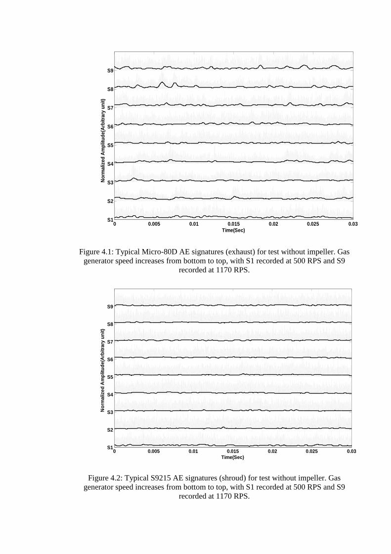
68
0 0.005 0.01 0.015 0.02 0.025 0.03S1
S2
S3
S4
S5
S6
S7
S8
S9
Time(Sec)
Nor
mal
ized
Am
plitu
de(A
rbitr
ary
unit)
Figure 4.1: Typical Micro-80D AE signatures (exhaust) for test without impeller. Gas generator speed increases from bottom to top, with S1 recorded at 500 RPS and S9
recorded at 1170 RPS.
0 0.005 0.01 0.015 0.02 0.025 0.03S1
S2
S3
S4
S5
S6
S7
S8
S9
Time(Sec)
No
rmal
ized
Am
plit
ud
e(A
rbitr
ary
un
it)
Figure 4.2: Typical S9215 AE signatures (shroud) for test without impeller. Gas generator speed increases from bottom to top, with S1 recorded at 500 RPS and S9
recorded at 1170 RPS.

69
Figures 4.3 and 4.4 show the evolution of AE energy with gas generator speed for the
exhaust and turbine shroud sensors, respectively. Each point represents the energy
content of the record using equation 2.4 and all 20 values are shown at each speed for
each of the two tests. As can be seen, the AE energy at a given speed seems consistent
between the records (each of which accounts for typically 15-33 revolutions of the
machine) but there is a marked variation in the level of energy between the two tests for
the exhaust-mounted sensor, not reflected in the record for the shroud-mounted sensor.
Given that the surface of the shroud is hot, it is possible that this variation was due to
some degradation of the coupling between the two tests. Notwithstanding this, both
sensors indicate an increase in AE energy with a speed of an increasing slope, fitted
here using an exponential growth function. It might also be noted that the energy
recorded on the shroud is a factor of 50-100 lower than that recorded at the exhaust,
which is approximately the same as the ratio of the sensitivities of the two sensors when
both are mounted on the turbine shroud (cold) and on the steel block.
Figures 4.5 (a) and (b) show typical raw AE spectra for the nine speeds for the Micro-
80D and S9215 sensors, respectively. These spectra have been normalized across the
relevant filter bandwidth so that the effect of the absolute energy does not mask the
frequency content. The effect of the different analogue filters and sensor bandwidths is
immediately apparent in the two sensor responses, with significant energy being shown
by the S2915 sensor in the 0.05 to 0.1MHz range, just below the analogue filter cut-off
for the Micro-80D sensor. Despite this, both the Micro-80D and S2915 sensors show a
very strong peak at around 7.5kHz at some speeds which must be very strong indeed to
be able to penetrate the filter. Within its bandwidth, the Micro-80D shows a general
narrowing of the frequency content of the signal toward the bottom end of the filter
band-pass, and this probably indicates a shift to frequencies below 0.1MHz. Conversely,
the S9210 sensor shows a (less marked) migration of the frequency content towards a
band between 80 and 100kHz.
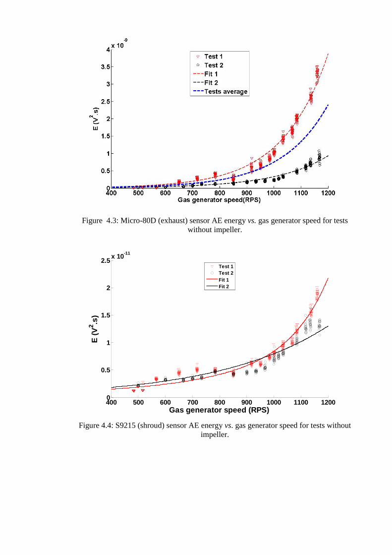
70
Figure 4.3: Micro-80D (exhaust) sensor AE energy vs. gas generator speed for tests without impeller.
400 500 600 700 800 900 1000 1100 12000
0.5
1
1.5
2
2.5x 10
-11
Gas generator speed (RPS)
E (
V2 .s
)
Test 1Test 2Fit 1Fit 2
Figure 4.4: S9215 (shroud) sensor AE energy vs. gas generator speed for tests without impeller.
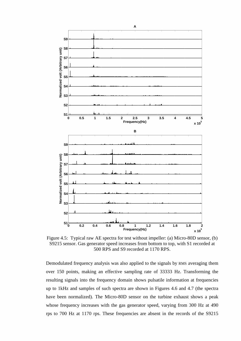
71
0 0.5 1 1.5 2 2.5 3 3.5 4 4.5 5
x 105
S1
S2
S3
S4
S5
S6
S7
S8
S9
Frequency(Hz)
No
rmal
ized
vo
lt (
Arb
itra
ry u
nit
)
A
0 0.2 0.4 0.6 0.8 1 1.2 1.4 1.6 1.8 2
x 105
S1
S2
S3
S4
S5
S6
S7
S8
S9
Frequency(Hz)
No
rmal
ized
vo
lt (
Arb
itra
ry u
nit
)
B
Figure 4.5: Typical raw AE spectra for test without impeller: (a) Micro-80D sensor, (b)
S9215 sensor. Gas generator speed increases from bottom to top, with S1 recorded at 500 RPS and S9 recorded at 1170 RPS.
Demodulated frequency analysis was also applied to the signals by RMS averaging them
over 150 points, making an effective sampling rate of 33333 Hz. Transforming the
resulting signals into the frequency domain shows pulsatile information at frequencies
up to 1kHz and samples of such spectra are shown in Figures 4.6 and 4.7 (the spectra
have been normalized). The Micro-80D sensor on the turbine exhaust shows a peak
whose frequency increases with the gas generator speed, varying from 300 Hz at 490
rps to 700 Hz at 1170 rps. These frequencies are absent in the records of the S9215

72
sensor mounted on the turbine shroud. Table 4.2 shows the running speed of gas
generator turbine of without impeller test.
Table 4. 2: Gas generator speed of without impeller test1.
Without impeller test speed Gas generator speed (RPS) S1 500 S2 600 S3 667 S4 700 S5 734 S6 784 S7 850 S8 900 S9 934 S10 967 S11 1000 S12 1017 S13 1034 S14 1083 S15 1117 S16 1133 S17 1167

73
0 100 200 300 400 500 600 700 800 900 1000S1
S2
S3
S4
S5
S6
S7
S8
S9
S10
S11
S12
S13
S14
S15
S16
S17
Frequency(Hz)
No
rma
lize
d v
olt
(Arb
itra
ry u
nit)
Figure 4.6: Typical demodulated AE spectra for test without impeller with Micro-80D sensor. Gas generator speed increases from bottom to top, with S1 recorded at 500 RPS
and S17 recorded at 1170 RPS.
0 100 200 300 400 500 600 700 800 900 1000S1
S2
S3
S4
S5
S6
S7
S8
S9
S10
S11
S12
S13
S14
S15
S16
S17
Frequency(Hz)
No
rmal
ized
vo
lt (A
rbitr
ary
un
it)
Figure 4.7: Typical demodulated AE spectra for test without impeller with S9215
sensor. Gas generator speed increases from bottom to top, with S1 recorded at 500 RPS and S17 recorded at 1170 RPS.
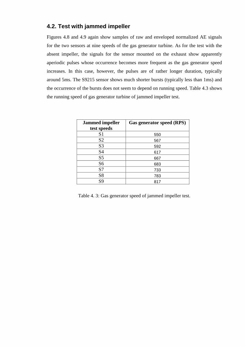
74
4.2. Test with jammed impeller
Figures 4.8 and 4.9 again show samples of raw and enveloped normalized AE signals
for the two sensors at nine speeds of the gas generator turbine. As for the test with the
absent impeller, the signals for the sensor mounted on the exhaust show apparently
aperiodic pulses whose occurrence becomes more frequent as the gas generator speed
increases. In this case, however, the pulses are of rather longer duration, typically
around 5ms. The S9215 sensor shows much shorter bursts (typically less than 1ms) and
the occurrence of the bursts does not seem to depend on running speed. Table 4.3 shows
the running speed of gas generator turbine of jammed impeller test.
Jammed impeller test speeds
Gas generator speed (RPS)
S1 550 S2 567 S3 592 S4 617 S5 667 S6 683 S7 733 S8 783 S9 817
Table 4. 3: Gas generator speed of jammed impeller test.

75
0 0.005 0.01 0.015 0.02 0.025 0.03S1
S2
S3
S4
S5
S6
S7
S8
S9
Time(Sec)
No
rmal
ized
Am
plit
ud
e(A
rbitr
ary
un
it)
Figure 4.8: Typical Micro-80D AE signatures for jammed impeller test. Gas generator speed increases from bottom to top, with S1 recorded at 500 RPS and S9 recorded at
850 RPS.
0 0.005 0.01 0.015 0.02 0.025 0.03S1
S2
S3
S4
S5
S6
S7
S8
S9
Time(Sec)
No
rmal
ized
Am
plit
ude
(Arb
itrar
y un
it)
Figure 4.9: Typical S9215 AE signatures for jammed impeller test. Gas generator speed increases from bottom to top, with S1 recorded at 500 RPS and S9 recorded at 850 RPS. Figures 4.10 and 4.11 show the evolution of AE energy with gas generator speed for the
two AE sensors. The two tests give repeatable results and, as for the test with the
impeller absent, there is a monotonic increase in energy with gas generator speed.
Unlike the test with the impeller absent, the energy recorded at the two sensors is of

76
approximately the same magnitude indicating a shift in the total energy of the source
away from the exhaust towards the shroud.
500 550 600 650 700 750 800 850 9000
1
2
3
4
5
6
7
8x 10
-9
Gas generator speed(RPS)
E(V
2 .S)
Test 1Test 2Fit 1Fit 2
Figure 4.10: Micro-80D (exhaust) sensor AE energy vs. gas generator speed for tests jammed impeller.
500 550 600 650 700 750 800 850 9000
0.2
0.4
0.6
0.8
1
1.2x 10
-8
Gas generator speed(RPS)
E(V
2 .S)
Test 1Test 2Fit 1Fit 4
.
Figure 4.11: S9215 (shroud) sensor AE energy vs. gas generator speed for tests jammed impeller.
Figure 4.12 shows samples of the normalised raw AE spectra across the relevant filter
bandwidth for nine speeds of the gas generator turbine for both sensors. Unlike the case
for the absent impeller, there is a systematic shift in AE energy towards the higher end

77
of the frequency band at around 350kHz. The energy recorded by the S9215 sensor is
focused in a narrow band around 27kHz and this does not appear to change much with
gas generator speed.
0 0.5 1 1.5 2 2.5 3 3.5 4 4.5 5
x 105
S1
S2
S3
S4
S5
S6
S7
S8
S9
Frequency(Hz)
No
rmal
ized
vo
lt (
Arb
itra
ry u
nit
)
A
0 0.2 0.4 0.6 0.8 1 1.2 1.4 1.6 1.8 2
x 105
S1
S2
S3
S4
S5
S6
S7
S8
S9
Frequency(Hz)
No
rmal
ized
vo
lt (
Arb
itra
ry u
nit
)
B
Figure 4.12: Typical raw AE spectra for test jammed impeller: (a) Micro-80D sensor, (b) S9215 sensor. Gas generator speed increases from bottom to top, with S1 recorded
at 500 RPS and S9 recorded at 850 RPS.
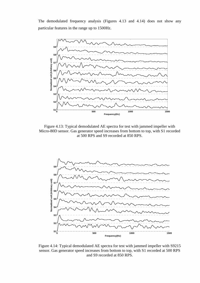
78
The demodulated frequency analysis (Figures 4.13 and 4.14) does not show any
particular features in the range up to 1500Hz.
0 500 1000 1500S1
S2
S3
S4
S5
S6
S7
S8
S9
Frequency(Hz)
No
rmal
ized
vo
lt (A
rbitr
ary
un
it)
Figure 4.13: Typical demodulated AE spectra for test with jammed impeller with Micro-80D sensor. Gas generator speed increases from bottom to top, with S1 recorded
at 500 RPS and S9 recorded at 850 RPS.
0 500 1000 1500S1
S2
S3
S4
S5
S6
S7
S8
S9
Frequency(Hz)
No
rmal
ized
vo
lt (A
rbitr
ary
un
it)
Figure 4.14: Typical demodulated AE spectra for test with jammed impeller with S9215 sensor. Gas generator speed increases from bottom to top, with S1 recorded at 500 RPS
and S9 recorded at 850 RPS.
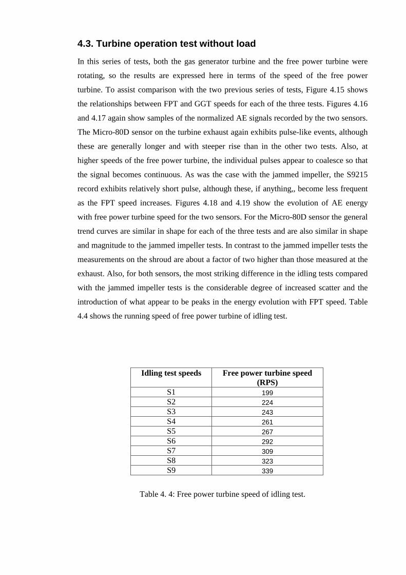
79
4.3. Turbine operation test without load
In this series of tests, both the gas generator turbine and the free power turbine were
rotating, so the results are expressed here in terms of the speed of the free power
turbine. To assist comparison with the two previous series of tests, Figure 4.15 shows
the relationships between FPT and GGT speeds for each of the three tests. Figures 4.16
and 4.17 again show samples of the normalized AE signals recorded by the two sensors.
The Micro-80D sensor on the turbine exhaust again exhibits pulse-like events, although
these are generally longer and with steeper rise than in the other two tests. Also, at
higher speeds of the free power turbine, the individual pulses appear to coalesce so that
the signal becomes continuous. As was the case with the jammed impeller, the S9215
record exhibits relatively short pulse, although these, if anything,, become less frequent
as the FPT speed increases. Figures 4.18 and 4.19 show the evolution of AE energy
with free power turbine speed for the two sensors. For the Micro-80D sensor the general
trend curves are similar in shape for each of the three tests and are also similar in shape
and magnitude to the jammed impeller tests. In contrast to the jammed impeller tests the
measurements on the shroud are about a factor of two higher than those measured at the
exhaust. Also, for both sensors, the most striking difference in the idling tests compared
with the jammed impeller tests is the considerable degree of increased scatter and the
introduction of what appear to be peaks in the energy evolution with FPT speed. Table
4.4 shows the running speed of free power turbine of idling test.
Idling test speeds Free power turbine speed (RPS)
S1 199 S2 224 S3 243 S4 261 S5 267 S6 292 S7 309 S8 323 S9 339
Table 4. 4: Free power turbine speed of idling test.

80
100 150 200 250 300 350 400200
250
300
350
400
450
500
550
600
650
700
Free power turbine speed (RPS)
Gas
gen
erat
or
spee
d (
RP
S)
Test 1Test 2Test 3Test average
Figure 4.15: Relationship between free power turbine speed and. gas generator speed for idling test.
0 0.005 0.01 0.015 0.02 0.025 0.03S1
S2
S3
S4
S5
S6
S7
S8
S9
Time(Sec)
Nor
mal
ized
Am
plitu
de(A
rbitr
ary
unit)
Figure 4.16: Typical Micro-80D AE signatures (exhaust) for test without load. Free power turbine speed increases from bottom to top, with S1 recorded at 140 RPS and S9
recorded at 345 RPS.

81
0 0.005 0.01 0.015 0.02 0.025 0.03S1
S2
S3
S4
S5
S6
S7
S8
S9
Time(Sec)
No
rmal
ized
Am
plit
ud
e(A
rbitr
ary
un
it)
Figure 4.17: Typical S9215 AE signatures (shroud) for test without load. Free power turbine speed increases from bottom to top, with S1 recorded at 140 RPS and S9
recorded at 345 RPS. .
100 150 200 250 300 3500
0.2
0.4
0.6
0.8
1
1.2
1.4
1.6
1.8x 10
-8
Free power turbine speed (RPS)
En
egry
(v2 .s
)
Test 1Test 2Test 3Fit 1Fit 2Fit 3
Figure 4.18: Micro-80D (exhaust) sensor AE energy vs. free power turbine speed for tests without load.

82
100 150 200 250 300 3500
0.5
1
1.5
2
2.5
3
3.5x 10
-8
Free power turbine speed(RPS)
En
egry
(v2 .s
)
Test 1Test 2Test 3Fit 1Fit 2Fit 3
Figure 4.19: S9215 (shroud) sensor AE energy vs. free power turbine speed for tests
without load.
Figure 4.20 shows a sample of raw AE spectra for the idling tests, with the Micro-80D
showing a gradual shift towards lower frequencies, and the S9215 sensor again showing
a narrow frequency range at around 35kHz with a slight tendency towards lower
frequencies at higher FPT speeds. Records from the turbine shroud show a similar
behavior at several points, i.e. S6, S8, and S9.
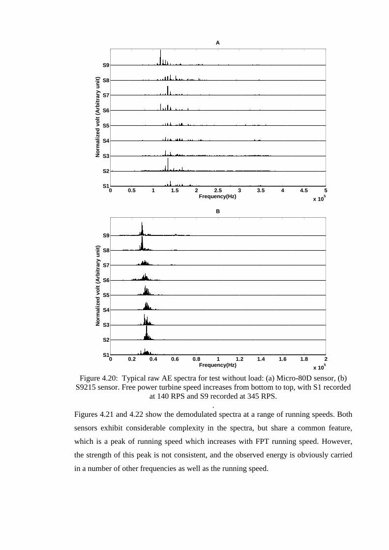
83
0 0.5 1 1.5 2 2.5 3 3.5 4 4.5 5
x 105
S1
S2
S3
S4
S5
S6
S7
S8
S9
Frequency(Hz)
No
rmal
ized
vo
lt (
Arb
itra
ry u
nit
)
A
0 0.2 0.4 0.6 0.8 1 1.2 1.4 1.6 1.8 2
x 105
S1
S2
S3
S4
S5
S6
S7
S8
S9
Frequency(Hz)
No
rmal
ized
vo
lt (
Arb
itra
ry u
nit
)
B
Figure 4.20: Typical raw AE spectra for test without load: (a) Micro-80D sensor, (b)
S9215 sensor. Free power turbine speed increases from bottom to top, with S1 recorded at 140 RPS and S9 recorded at 345 RPS.
. Figures 4.21 and 4.22 show the demodulated spectra at a range of running speeds. Both
sensors exhibit considerable complexity in the spectra, but share a common feature,
which is a peak of running speed which increases with FPT running speed. However,
the strength of this peak is not consistent, and the observed energy is obviously carried
in a number of other frequencies as well as the running speed.

84
0 200 400 600 800 1000 1200 1400 1600 1800 2000S1
S2
S3
S4
S5
S6
S7
S8
S9
Frequency(Hz)
No
rmal
ized
vo
lt (A
rbitr
ary
un
it)
Figure 4.21: Typical demodulated AE spectra for test without load with Micro-80D
sensor. Free power turbine speed increases from bottom to top, with S1 recorded at 140 RPS and S9 recorded at 345 RPS.
0 200 400 600 800 1000 1200 1400 1600 1800 2000S1
S2
S3
S4
S5
S6
S7
S8
S9
Frequency(Hz)
No
rmal
ized
vo
lt (A
rbitr
ary
un
it)
Figure 4.22: Typical demodulated AE spectra for test without load with S9215 sensor. Free power turbine speed increases from bottom to top, with S1 recorded at 140 RPS
and S9 recorded at 345 RPS.

85
4.4. Turbine operation test with load
This test involved adding a dynamic device i.e. the alternator, to the turbine rig in order
to study the changes in the AE behaviour when the FPT was subjected to an external
load, increased load being reflected in a reduced speed of the FPT. In this respect, the
signals were expected to be the most complex of the tests studied, but also those of most
relevance to real operations. A hint of this complexity is seen in Figures 4.23 and 4.24
where the examples of raw AE signals from two AE sensors show them all to contain
pulses, but with little obvious pattern in time or between running speeds. Table 4.5
shows the running speed of free power turbine of load test.
Load test speeds Free power turbine speed (RPS) S1 184 S2 206 S3 216 S4 231 S5 263 S6 275 S7 284 S8 301 S9 320
Table 4. 5: Free power turbine speed of load test.

86
0 0.005 0.01 0.015 0.02 0.025 0.03S1
S2
S3
S4
S5
S6
S7
S8
S9
Time(Sec)
Nor
mal
ized
Am
plitu
de(A
rbitr
ary
unit)
Figure 4.23: Typical Micro-80D AE signatures (exhaust) for test with load. Free power turbine speed increases from bottom to top, with S1 recorded at 150 RPS and S9
recorded at 360 RPS.
0 0.005 0.01 0.015 0.02 0.025 0.03S1
S2
S3
S4
S5
S6
S7
S8
S9
Time(Sec)
No
rmal
ized
Am
plit
ud
e(A
rbitr
ary
un
it)
Figure 4.24: Typical S9215 AE signatures (shroud) for test with load. Free power turbine speed increases from bottom to top, with S1 recorded at 150 RPS and S9
recorded at 360 RPS.

87
Figures 4.25 and 4.26 show the variation in AE energy with FPT speed for the two
sensors. The most striking features of these two curves are that they are up to two orders
of magnitude higher than the equivalent idling curves and that the curves are no longer
monotonic, with peaks in AE energy across the range of speed studied, the speeds at
which the peaks occur varying between the three individual tests. The energy levels
recorded at the shroud are generally an order of magnitude lower than those recorded at
the exhaust.
100 150 200 250 300 350 4000
0.5
1
1.5
2
2.5
3
3.5
4x 10
-6
Free power turbine speed(RPS)
En
erg
y(V
2 .S)
Test 1Test 2Test 3Fit 1Fit 2Fit 3
Figure 4.25: Micro-80D (exhaust) sensor AE energy vs. free power turbine speed for tests with load.
100 150 200 250 300 350 4000
0.5
1
1.5
2
2.5
3x 10
-7
Free power turbine speed(RPS)
En
erg
y(V
2 .S)
Test 1Test 2Test 3Fit 1Fit 2Fit 3
Figure 4.26: S9215 (shroud ) sensor AE energy vs. free power turbine speed for tests
with load.

88
Figure 4.27 shows sample raw AE spectra, those for the exhaust again showing a
tendency to drift towards the bottom of the analogue filter bandwidth as the speed
increases. The S9215 spectra show one peak at around 25kHz, which slowly moves
towards 20kHz as the speed increase with other peaks which appear and disappear with
speed.
0 0.5 1 1.5 2 2.5 3 3.5 4 4.5 5
x 105
S1
S2
S3
S4
S5
S6
S7
S8
S9
Frequency(Hz)
No
rmal
ized
vo
lt (
Arb
itra
ry u
nit
)
A
0 0.2 0.4 0.6 0.8 1 1.2 1.4 1.6 1.8 2
x 105
S1
S2
S3
S4
S5
S6
S7
S8
S9
Frequency(Hz)
No
rmal
ized
vo
lt (
Arb
itra
ry u
nit
)
B
Figure 4.27: Typical raw AE spectra for test with load: (a) Micro-80D sensor, (b) S9215 sensor. Free power turbine speed increases from bottom to top, with S1 recorded
at 150 RPS and S9 recorded at 360 RPS.

89
The demodulated frequency spectra in figures 4.28 and 4.29 both show a strong series
of peaks at the running speed frequency and its harmonics. Nevertheless, the strength of
these is again not consistent and a number of other, sometimes equally strong, peaks are
present.
0 200 400 600 800 1000 1200 1400 1600 1800 2000S1
S2
S3
S4
S5
S6
S7
S8
S9
Frequency(Hz)
No
rmal
ized
PS
D(A
rbitr
ary
un
it)
Figure 4.28: Typical demodulated AE spectra for test with load with Micro-80D sensor. Free power turbine speed increases from bottom to top, with S1 recorded at 150 RPS
and S9 recorded at 360 RPS.
0 200 400 600 800 1000 1200 1400 1600 1800 2000S1
S2
S3
S4
S5
S6
S7
S8
S9
Frequency (Hz)
No
rmal
ized
vo
lt (A
rbit
rary
un
it)
Figure 4.29: Typical demodulated AE spectra for test with load with S9215 sensor. Free power turbine speed increases from bottom to top, with S1 recorded at 150 RPS and S9
recorded at 360 RPS.

90
4.5. Summary
The initial analysis of the results in this section indicate that the complexity of the AE
signals increases with the complexity of the fluid-mechanics occurring within the free
power turbine and its exhaust, with both sensors yielding information which changes
with speed whilst each clearly is sensitive to different phenomena. The experiments
with the impeller stationary are the least complex and contain the least AE energy at a
given speed, indicating that much of the complexity and AE energy is associated with
the rotation of the FPT impeller. The fact that the signals are not wholly continuous
indicates a dynamic effect which potentially contains information over and above the
mean energy level. Table 4.6 shows AE energy average for all four tests. It is clear from
the table and the pervious energy graphs that the mean energy level is a poor indicator
of operating conditions when the turbine is under load and this is clearly associated with
the presence of pulses with frequencies in the range of a few tens to a few hundreds of
Hz. In view of the complex nature of the AE patterns, the next chapter will examine the
signals in more detail with the aid of an ANN algorithm.
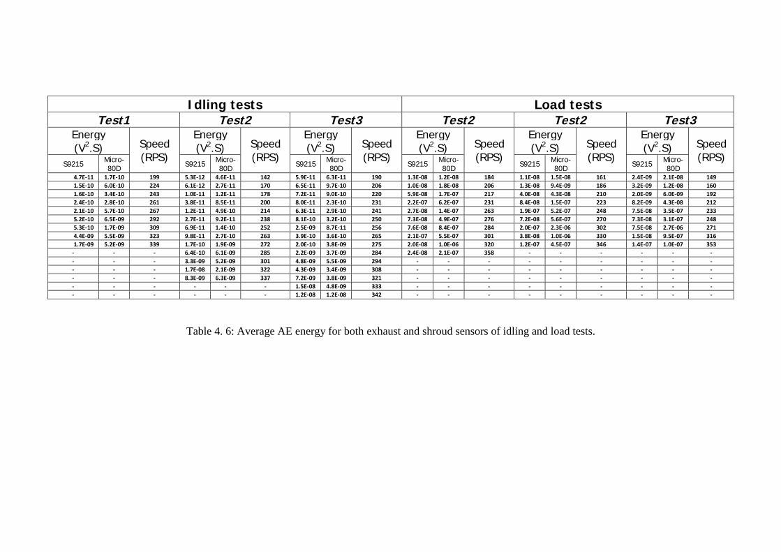
91
Table 4. 6: Average AE energy for both exhaust and shroud sensors of idling and load tests.
Idling tests Load tests Test1 Test2 Test3 Test2 Test2 Test3
Energy (V2.S) Speed
(RPS)
Energy (V2.S) Speed
(RPS)
Energy (V2.S) Speed
(RPS)
Energy (V2.S) Speed
(RPS)
Energy (V2.S) Speed
(RPS)
Energy (V2.S) Speed
(RPS) S9215 Micro-
80D S9215 Micro-80D S9215 Micro-
80D S9215 Micro-80D S9215 Micro-
80D S9215 Micro-80D
4.7E-11 1.7E-10 199 5.3E-12 4.6E-11 142 5.9E-11 6.3E-11 190 1.3E-08 1.2E-08 184 1.1E-08 1.5E-08 161 2.4E-09 2.1E-08 149 1.5E-10 6.0E-10 224 6.1E-12 2.7E-11 170 6.5E-11 9.7E-10 206 1.0E-08 1.8E-08 206 1.3E-08 9.4E-09 186 3.2E-09 1.2E-08 160 1.6E-10 3.4E-10 243 1.0E-11 1.2E-11 178 7.2E-11 9.0E-10 220 5.9E-08 1.7E-07 217 4.0E-08 4.3E-08 210 2.0E-09 6.0E-09 192 2.4E-10 2.8E-10 261 3.8E-11 8.5E-11 200 8.0E-11 2.3E-10 231 2.2E-07 6.2E-07 231 8.4E-08 1.5E-07 223 8.2E-09 4.3E-08 212 2.1E-10 5.7E-10 267 1.2E-11 4.9E-10 214 6.3E-11 2.9E-10 241 2.7E-08 1.4E-07 263 1.9E-07 5.2E-07 248 7.5E-08 3.5E-07 233 5.2E-10 6.5E-09 292 2.7E-11 9.2E-11 238 8.1E-10 3.2E-10 250 7.3E-08 4.9E-07 276 7.2E-08 5.6E-07 270 7.3E-08 3.1E-07 248 5.3E-10 1.7E-09 309 6.9E-11 1.4E-10 252 2.5E-09 8.7E-11 256 7.6E-08 8.4E-07 284 2.0E-07 2.3E-06 302 7.5E-08 2.7E-06 271 4.4E-09 5.5E-09 323 9.8E-11 2.7E-10 263 3.9E-10 3.6E-10 265 2.1E-07 5.5E-07 301 3.8E-08 1.0E-06 330 1.5E-08 9.5E-07 316 1.7E-09 5.2E-09 339 1.7E-10 1.9E-09 272 2.0E-10 3.8E-09 275 2.0E-08 1.0E-06 320 1.2E-07 4.5E-07 346 1.4E-07 1.0E-07 353
- - - 6.4E-10 6.1E-09 285 2.2E-09 3.7E-09 284 2.4E-08 2.1E-07 358 - - - - - - - - - 3.3E-09 5.2E-09 301 4.8E-09 5.5E-09 294 - - - - - - - - - - - - 1.7E-08 2.1E-09 322 4.3E-09 3.4E-09 308 - - - - - - - - - - - - 8.3E-09 6.3E-09 337 7.2E-09 3.8E-09 321 - - - - - - - - - - - - - - - 1.5E-08 4.8E-09 333 - - - - - - - - - - - - - - - 1.2E-08 1.2E-08 342 - - - - - - - - -

92
Chapter 5 Analysis and discussion of normal running tests
The foregoing chapter has shown that the evolution of AE energy with turbine running
speed is relatively simple when the gas flow is simple, but that the energy evolutions
become non-monotonic when the impeller is rotating and more so when the turbine is
under load.
This chapter focuses on a more detailed analysis of the two tests with a rotating
impeller, idling and with the FPT under load. Because the AE patterns are complex, a
pattern recognition approach has been taken based on the observations made in chapter
4. Also, because the requirement is to understand the changing characteristics of the AE
with normal running operating conditions the focus of the pattern recognition has been
the turbine running speed.
The analysis is divided into three parts, time domain processing, frequency domain
processing and, finally, an approach that combines features from both time and
frequency domains
5.1. Time domain analysis
As observed in chapter 4 the AE time series signals at various speeds both with and
without load are not obviously periodic but exhibit pulses on a background continuous
signal. Therefore a processing approach was devised, based on a categorisation of pulse
shape, and this was applied to the idling tests. Next, a more statistical approach was
taken, whereby a wide range of time-based features was extracted and these were tested
using an ANN.
5.1.1. Pulse shape categorisation Here the aim was to categorise the bursts and to describe their temporal distribution to
examine if this was characteristic of the running conditions. To this end, AE signals
were examined visually in the time domain and four distinct shapes of envelope were
identified for each of the sensors/positions, Figures 5.1 and 5.2.
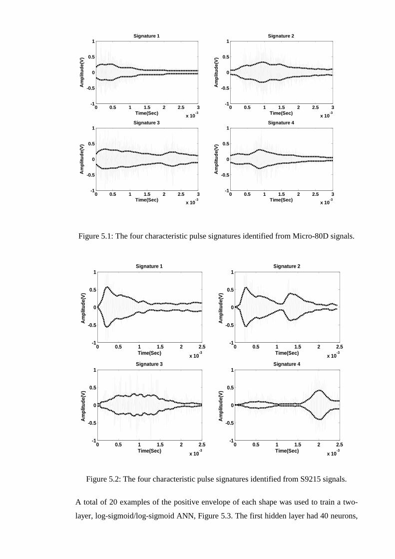
93
Figure 5.1: The four characteristic pulse signatures identified from Micro-80D signals.
Figure 5.2: The four characteristic pulse signatures identified from S9215 signals.
A total of 20 examples of the positive envelope of each shape was used to train a two-
layer, log-sigmoid/log-sigmoid ANN, Figure 5.3. The first hidden layer had 40 neurons,
0 0.5 1 1.5 2 2.5 3
x 10-3
-1
-0.5
0
0.5
1Signature 1
Time(Sec)
Am
plit
ud
e(V
)
0 0.5 1 1.5 2 2.5 3
x 10-3
-1
-0.5
0
0.5
1Signature 2
Time(Sec)
Am
plit
ud
e(V
)
0 0.5 1 1.5 2 2.5 3
x 10-3
-1
-0.5
0
0.5
1Signature 3
Time(Sec)
Am
plit
ud
e(V
)
0 0.5 1 1.5 2 2.5 3
x 10-3
-1
-0.5
0
0.5
1Signature 4
Time(Sec)
Am
plit
ud
e(V
)
0 0.5 1 1.5 2 2.5
x 10-3
-1
-0.5
0
0.5
1
Time(Sec)
Am
plit
ud
e(V
)
Signature 1
0 0.5 1 1.5 2 2.5
x 10-3
-1
-0.5
0
0.5
1
Time(Sec)
Am
plit
ud
e(V
)
Signature 2
0 0.5 1 1.5 2 2.5
x 10-3
-1
-0.5
0
0.5
1
Time(Sec)
Am
plit
ud
e(V
)
Signature 3
0 0.5 1 1.5 2 2.5
x 10-3
-1
-0.5
0
0.5
1
Time(Sec)
Am
plit
ud
e(V
)
Signature 4
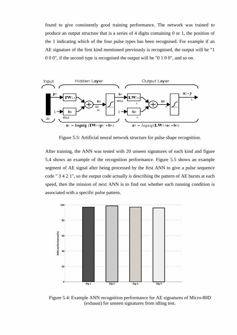
94
found to give consistently good training performance. The network was trained to
produce an output structure that is a series of 4 digits containing 0 or 1, the position of
the 1 indicating which of the four pulse types has been recognised. For example if an
AE signature of the first kind mentioned previously is recognised, the output will be "1
0 0 0", if the second type is recognised the output will be "0 1 0 0", and so on.
Figure 5.3: Artificial neural network structure for pulse shape recognition.
After training, the ANN was tested with 20 unseen signatures of each kind and figure
5.4 shows an example of the recognition performance. Figure 5.5 shows an example
segment of AE signal after being processed by the first ANN to give a pulse sequence
code " 3 4 2 1", so the output code actually is describing the pattern of AE bursts at each
speed, then the mission of next ANN is to find out whether each running condition is
associated with a specific pulse pattern.
Sig 1 Sig 2 Sig 3 Sig 40
20
40
60
80
100
AN
N p
erf
orm
ance
(%)
Figure 5.4: Example ANN recognition performance for AE signatures of Micro-80D (exhaust) for unseen signatures from idling test.

95
Figure 5.5: Sample coded signal for pulse shape recognition of Micro-80D (exhaust)
sensor for idling test. The number of pulses in each record will change depending on the turbine speed; for
instance, each record contains 5 pulses at a speed of 150 RPS and 8 pulses at a speed of
300 RPS. The longer records were truncated to the first 5 pulses to build a suitable input
to the ANN. The resulting data for both sensors for each speed of the idling test were
divided into two equal parts, one for training and one for testing, as input to a second
neural network whose output was the running speed. This was a feed-forward, back-
propagation ANN with two-layers. The hidden layer again used 40 neurons and a log-
sigmoid transfer function. The transfer function for the output layer was also a log-
sigmoid and the number of neurons in this layer was equal to the number of speeds to
which the network was to be trained. Figures 5.6 and 5.7 show the resulting
performance, as percentage speed correct classification, for each sensor, and for the
three individual tests and for the three tests collectively.

96
Test 1 Test 2 Test 3 All Tests0
20
40
60
80
100
AN
N p
erfo
rman
ce(%
)
Figure 5.6: Pulse shape recognition ANN performance for Micro-80D (exhaust) data from idling tests.
Test 1 Test 2 Test 3 All Tests0
20
40
60
80
100
AN
N p
erfo
rman
ce(%
)
Figure 5.7: Pulse shape recognition ANN performance for S9215 (shroud) data from idling tests.
As can be seen, the performance of the pulse shape network was poor, so the input was
improved by adding information about the time between pulses. The input codes were
modified to include the time differences between each pulse and the network was

97
trained and tested again with the new input data. Figures 5.8 and 5.9 show that there
was a general improvement in the performance of the updated network, but this is still
relatively poor at around 60% correct speed classification for the individual tests and
around 40% for the tests grouped together.
Test 1 Test 2 Test 3 All Tests0
20
40
60
80
100
AN
N p
erfo
rman
ce(%
)
Figure 5.8: Improved pulse shape recognition ANN performance for Micro-80D (exhaust) data from idling tests.
Test 1 Test 2 Test 3 All Tests0
20
40
60
80
100
AN
N p
erfo
rman
ce(%
)
Figure 5.9: improved pulse shape recognition ANN performance for S9215 (shroud)
data from idling tests.

98
5.1.2. Statistical time feature classification
In view of the poor performance of the pulse recognition techniques, it was decided to
extract the maximum possible amount of information from the time domain. To this end
a range of features; energy, maximum amplitude, counts, RMS, mean, standard
deviation, skew, and kurtosis, were generated from the time series in the interest of
describing the signals as fully as possible. Also, the static neural network, where the
output is calculated directly from the input through feed-forward connections, was
replaced with a dynamic network. The output of a dynamic network depends not only
on the current input but also on previous inputs, outputs, or states of the network, i.e. it
has a memory and its response at any given time depends not only on the current input
but also on the history of the input sequence. The implementation used consisted of one
log-sigmoid layer with 20 neurons with a feed-forward, back-propagation learning
algorithm again with the output consisting of the running speed, one node being
allocated to each speed used. As before, half of the data set was used to train the
network to the measured running speed. The network was then tested, delivering
weights to the output nodes from which a speed classification could be obtained (most
highly weighted output node) and an estimate of running speed (weighted mean of all
output nodes). Figure 5.10 shows the resulting ANN performance with time domain
features for each of the sensor records acquired on the running turbine with and without
load. As before, the ANN was applied to the data from the three individual tests and
again on data from the three tests mixed together. The performance figure is the
percentage of times that a test speed is correctly classified.

99
Test 1 Test 2 Test 3 All Tests0
10
30
50
70
90
a
AN
N P
erfo
rman
ce(%
)
Test 1 Test 2 Test 3 All Tests0
10
30
50
70
90
b
AN
N P
erfo
rman
ce(%
)
Test 1 Test 2 Test 3 All Tests0
10
30
50
70
90
c
AN
N P
erfo
rman
ce(%
)
Test 1 Test 2 Test 3 All Tests0
10
30
50
70
90
d
AN
N P
erfo
rman
ce(%
)
Figure 5.10: ANN classification performance using all statistical time features: (a)
S9215 sensor, idling tests, (b) Micro-80D sensor, idling tests, (c) S9215 sensor, load tests, (d) Micro-80D sensor, load tests.
Figure 5.10 shows good performance for the individual tests, but poorer performance
for the collected data. Figures 5.11 to 5.13 show the weighted output of the ANN
compared with the measured turbine speed. The weighted output provides an estimate
of the speed which takes account of the weights of each output neuron (as opposed to
the value at maximum weight, i.e. the classification). The red points on the graphs
represent the actual running speed whereas the blue points represent the estimated
running speed. Presentation of the data in this form allows a number of additional
observations, such as the generally higher level of certainty in the load tests and the
tendency to over-estimate the actual speed when all tests are grouped.

100
0 20 40 60 80 100150
200
250
300
350Test 1
Record number
Sp
eed
(RP
S)
0 50 100 150100
150
200
250
300
350Test 2
Record number
Sp
eed
(RP
S)
0 50 100 150150
200
250
300
350Test 3
Record number
Sp
eed
(RP
S)
0 100 200 300 400100
150
200
250
300
350
400All tests
Record number
Sp
eed
(RP
S)
ANN speed
Real speed
ANN speed
Real speed
ANN speed
Real speed
ANN speed
Real speed
Figure 5.11: ANN speed estimate error for S9215 sensor idling test.
0 20 40 60 80 100150
200
250
300
350
Record number
Sp
eed
(RP
S)
Test 1
0 50 100 150100
150
200
250
300
350
Record number
Sp
eed
(RP
S)
Test 2
0 50 100 150150
200
250
300
350Test 3
Record number
Sp
eed
(RP
S)
0 100 200 300 400100
150
200
250
300
350
400All tests
Record number
Sp
eed
(RP
S)
ANN speedReal speed
ANN speedReal speed
ANN speedReal speed
ANN speedReal speed
Figure 5.12: ANN speed estimate error for Micro-80D sensor on idling test.

101
0 20 40 60 80 100150
200
250
300
350
400
Record number
Sp
eed
(RP
S)
Test 1
0 20 40 60 80 100150
200
250
300
350Test 2
Record number
Sp
eed
(RP
S)
0 20 40 60 80 100100
150
200
250
300
350
400
Record number
Sp
eed(
RP
S)
Test 3
0 50 100 150 200 250 300100
150
200
250
300
350
400
Record number
Sp
eed(
RP
S)
All tests
ANN speedReal speed
ANN speedReal speed
ANN speedReal speed
ANN speedReal speed
Figure 5.13: ANN speed estimate error for S9215 sensor on load test.
0 20 40 60 80 100150
200
250
300
350
400Test 1
Record number
Sp
eed
(RP
S)
0 20 40 60 80 100150
200
250
300
350Test 2
Record number
Sp
eed
(RP
S)
0 20 40 60 80 100100
150
200
250
300
350
400Test 3
Record number
Sp
eed
(RP
S)
0 50 100 150 200 250 300100
150
200
250
300
350
400All tests
Record number
Sp
eed
(RP
S)
ANN speedReal speed
ANN speedReal speed
ANN speedReal speed
ANN speedReal speed
Figure 5.14: ANN speed estimate error for Micro-80D sensor on load test.
Although the ANN performance for individual tests with all time features was over
75%, the features driving that performance were not yet known. Accordingly, the ANN

102
was trained and tested with each individual time feature in order to identify the most
efficient time features in pattern recognition. Figures 5.15 and 5.16 show the resulting
ANN performance and show two clear groups, those with high discriminating power
(STD, RMS, Max amp, Counts, and Energy), and those with low discriminating power
group (Skew, Kurtosis and Mean).
Energy Counts Max Amp RMS Mean STD Skew Kurt0
20
40
60
80
100(a)
AN
N P
erfo
rman
ce(%
)
Energy Counts Max Amp RMS Mean STD Skew Kurt0
20
40
60
80
100(b)
AN
N P
erfo
rman
ce(%
)
Test 1Test 2Test 3All test
Test 1Test 2Test 3All test
Figure 5.15: ANN performance for individual time features derived from idling test: (a) S9215 sensor,(b) Micro-80D sensor.
Energy Counts Max Amp RMS Mean STD Skew Kurt0
20
40
60
80
100(a)
AN
N P
erf
orm
an
ce
(%)
Energy Counts Max Amp RMS Mean STD Skew Kurt0
20
40
60
80
100(b)
AN
N P
erf
orm
an
ce
(%)
Test 1Test 2Test 3All Test
Test 1Test 2Test 3All test
Figure 5.16: ANN performance for individual time features derived from without load test: (a) S9215 sensor,(b) Micro-80D sensor.
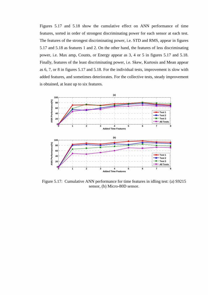
103
Figures 5.17 and 5.18 show the cumulative effect on ANN performance of time
features, sorted in order of strongest discriminating power for each sensor at each test.
The features of the strongest discriminating power, i.e. STD and RMS, appear in figures
5.17 and 5.18 as features 1 and 2. On the other hand, the features of less discriminating
power, i.e. Max amp, Counts, or Energy appear as 3, 4 or 5 in figures 5.17 and 5.18.
Finally, features of the least discriminating power, i.e. Skew, Kurtosis and Mean appear
as 6, 7, or 8 in figures 5.17 and 5.18. For the individual tests, improvement is slow with
added features, and sometimes deteriorates. For the collective tests, steady improvement
is obtained, at least up to six features.
0 1 2 3 4 5 6 7 80
20
40
60
80
100
Added Time Features
AN
N P
erfo
rman
ce(%
)
(a)
Test 1Test 2Test 3All Tests
0 1 2 3 4 5 6 7 80
20
40
60
80
100
Added Time Features
AN
N P
erfo
rman
ce(%
)
(b)
Test 1Test 2Test 3All Tests
Figure 5.17: Cumulative ANN performance for time features in idling test: (a) S9215
sensor, (b) Micro-80D sensor.
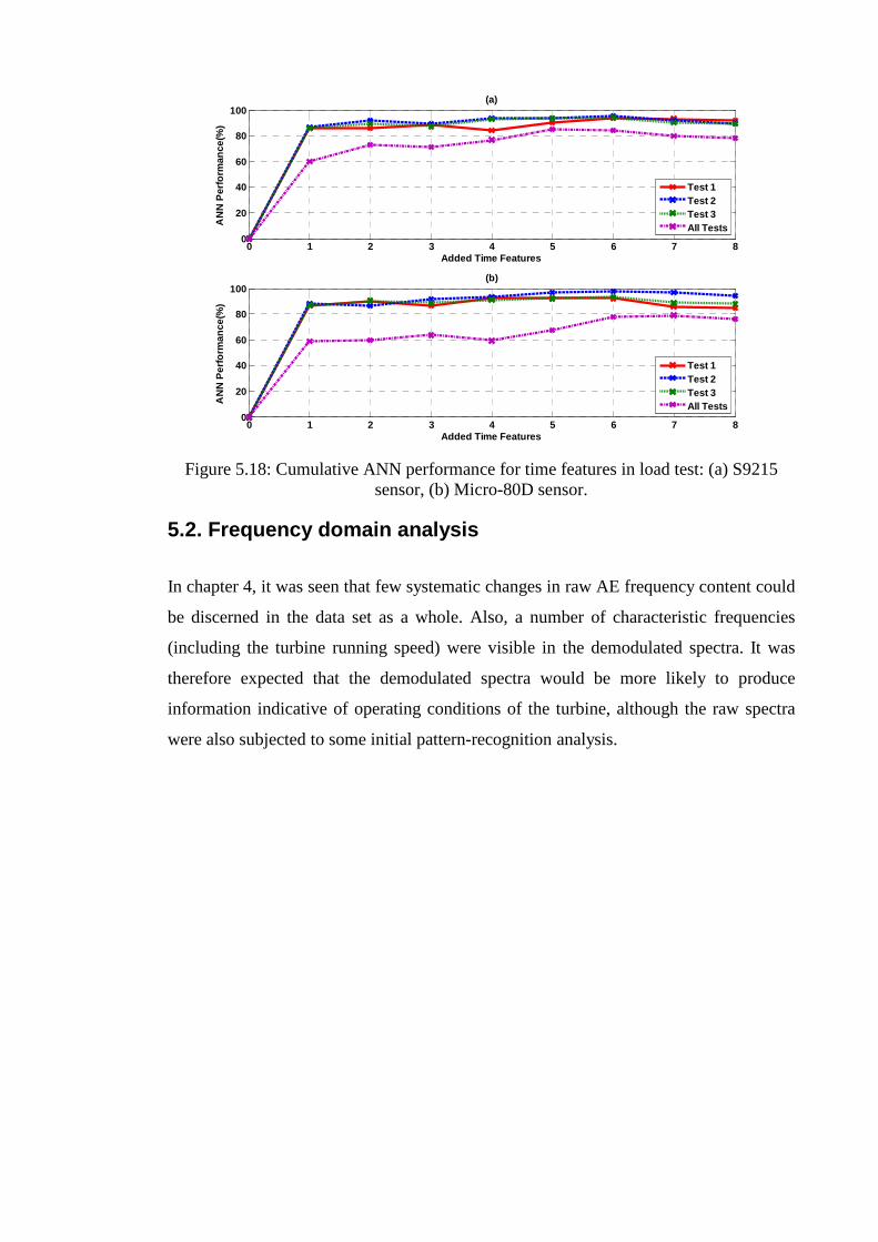
104
0 1 2 3 4 5 6 7 80
20
40
60
80
100
Added Time Features
AN
N P
erfo
rman
ce(%
)
(a)
Test 1Test 2Test 3All Tests
0 1 2 3 4 5 6 7 80
20
40
60
80
100
Added Time Features
AN
N P
erfo
rman
ce(%
)
(b)
Test 1Test 2Test 3All Tests
Figure 5.18: Cumulative ANN performance for time features in load test: (a) S9215
sensor, (b) Micro-80D sensor.
5.2. Frequency domain analysis
In chapter 4, it was seen that few systematic changes in raw AE frequency content could
be discerned in the data set as a whole. Also, a number of characteristic frequencies
(including the turbine running speed) were visible in the demodulated spectra. It was
therefore expected that the demodulated spectra would be more likely to produce
information indicative of operating conditions of the turbine, although the raw spectra
were also subjected to some initial pattern-recognition analysis.

105
5.2.1. Raw frequency classification
On the basis of an examination of figures 4.19 and 4.26, five features were extracted
from the raw frequency domain: (a) the ratio of the energies in a low frequency band
(100-200 kHz) to a high frequency band (300-450kHz), (b) the standard deviation of the
spectrum, (c) the maximum amplitude of the spectrum, (d) the frequency at maximum
amplitude, and (e) the frequency skewness. Values of these frequency features from the
idling tests were split into two equal parts, as before, and the network trained to
recognize the running speed, performance being measured by the proportion of correct
classifications in the test set. Figure 5.19 shows the classification performance for both
the Micro-80D and S9215 sensors. As expected, this shows a relatively poor
classification for both sensors.
Test 1 Test 2 Test 3 All Tests0
20
40
60
80
100
AN
N P
erfo
rman
ce(%
)
(a)
Test 1 Test 2 Test 3 All Tests0
20
40
60
80
100(b)
AN
N P
erfo
rman
ce(%
)
Figure 5.19: ANN performance for without load tests of frequency features (a) Micro-
80D sensor performance (b) S9215 sensor performance.
5.2.2. Demodulated frequency spectra
Figures 5.20 and 5.21 show all of the demodulated spectra recorded in the idling tests
for the exhaust-mounted sensor and the shroud-mounted sensor, respectively. All
spectra were normalised to the energy content to facilitate comparison and averaging
and avoid the complication of including the energy or amplitude of the signal which is
the subject of the analysis in the previous section. Each of the independent sample
spectra are shown in blue and the averaged spectra are shown as heavy red dotted lines.

106
As can be seen, many of the averaged spectra show a clear peak at the running speed
(arrowed in Figures 5.20 and 5.21), and, less often, the first harmonic of the running
speed. However, the running speed is rarely the dominant peak in the spectrum and, in
cases where its peak is weak or absent, the individual spectra which make up the
average often contain strong peaks at a very wide range of frequencies. Many of the
exhaust spectra contain a strong peak at around 110Hz, sometimes associated with
peaks either side at around 40Hz and 165Hz. The 110Hz peak tends to be more strongly
exhibited at the exhaust, whereas the running speed peaks tend to be more strongly
exhibited at the shroud.

107
0 200 400 600 800 10000
0.002
0.004
0.006
0.008
0.01
0.012
Frequency(Hz)
Am
plit
ud
e(V
)
FPT speed(199 RPS)
0 200 400 600 800 10000
0.002
0.004
0.006
0.008
0.01
Frequency(Hz)
Am
plit
ud
e(V
)
FPT speed(242 RPS)
0 200 400 600 800 10000
0.002
0.004
0.006
0.008
0.01
Frequency(Hz)
Am
plit
ud
e(V
)
FPT speed(260 RPS)
0 200 400 600 800 10000
0.005
0.01
0.015
Frequency(Hz)
Am
plit
ud
e(V
)
FPT speed(268 RPS)
Running speed
Running speed harmonic
0 200 400 600 800 10000
1
2
3
4
5
6
x 10-3
Frequency(Hz)
Am
plit
ud
e(V
)
FPT speed(308 RPS)
0 200 400 600 800 10000
2
4
6
8
x 10-3
Frequency(Hz)
Am
plit
ud
e(V
)
FPT speed(323 RPS)
0 200 400 600 800 10000
0.002
0.004
0.006
0.008
0.01
0.012
Frequency(Hz)
Am
plit
ud
e(V
)
FPT speed(340 RPS)
0 200 400 600 800 10000
0.002
0.004
0.006
0.008
0.01
0.012
Frequency(Hz)
Am
plit
ud
e(V
)
FPT speed(291 RPS)
100 Hz frequency
Figure 5.20: Demodulated spectra for idling test with Micro-80D sensor at 8 different speeds of FPT. Individual spectra shown in blue and averaged spectra shown in red.
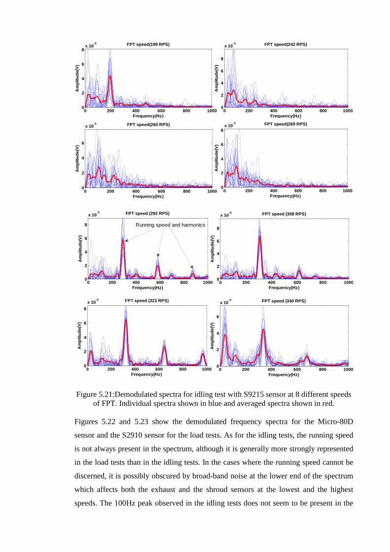
108
0 200 400 600 800 10000
2
4
6
8x 10
-3
Frequency(Hz)
Am
plit
ud
e(V
)
FPT speed(199 RPS)
0 200 400 600 800 10000
2
4
6
8
x 10-3
Frequency(Hz)
Am
plit
ud
e(V
)
FPT speed(242 RPS)
0 200 400 600 800 10000
2
4
6
x 10-3
Frequency(Hz)
Am
plit
ud
e(V
)
FPT speed(260 RPS)
0 200 400 600 800 10000
2
4
6
8x 10
-3
Frequency(Hz)
Am
plit
ud
e(V
)
FPT speed(269 RPS)
0 200 400 600 800 10000
2
4
6
8
x 10-3
Frequency(Hz)
Am
plit
ud
e(V
)FPT speed (308 RPS)
0 200 400 600 800 10000
2
4
6
8
x 10-3
Frequency(Hz)
Am
plit
ud
e(V
)
FPT speed (323 RPS)
0 200 400 600 800 10000
2
4
6
x 10-3
Frequency(Hz)
Am
plit
ud
e(V
)
FPT speed (340 RPS)
0 200 400 600 800 10000
2
4
6
8
x 10-3
Frequency(Hz)
Am
plit
ud
e(V
)
FPT speed (292 RPS)
Running speed and harmonics
Figure 5.21:Demodulated spectra for idling test with S9215 sensor at 8 different speeds of FPT. Individual spectra shown in blue and averaged spectra shown in red.
Figures 5.22 and 5.23 show the demodulated frequency spectra for the Micro-80D
sensor and the S2910 sensor for the load tests. As for the idling tests, the running speed
is not always present in the spectrum, although it is generally more strongly represented
in the load tests than in the idling tests. In the cases where the running speed cannot be
discerned, it is possibly obscured by broad-band noise at the lower end of the spectrum
which affects both the exhaust and the shroud sensors at the lowest and the highest
speeds. The 100Hz peak observed in the idling tests does not seem to be present in the
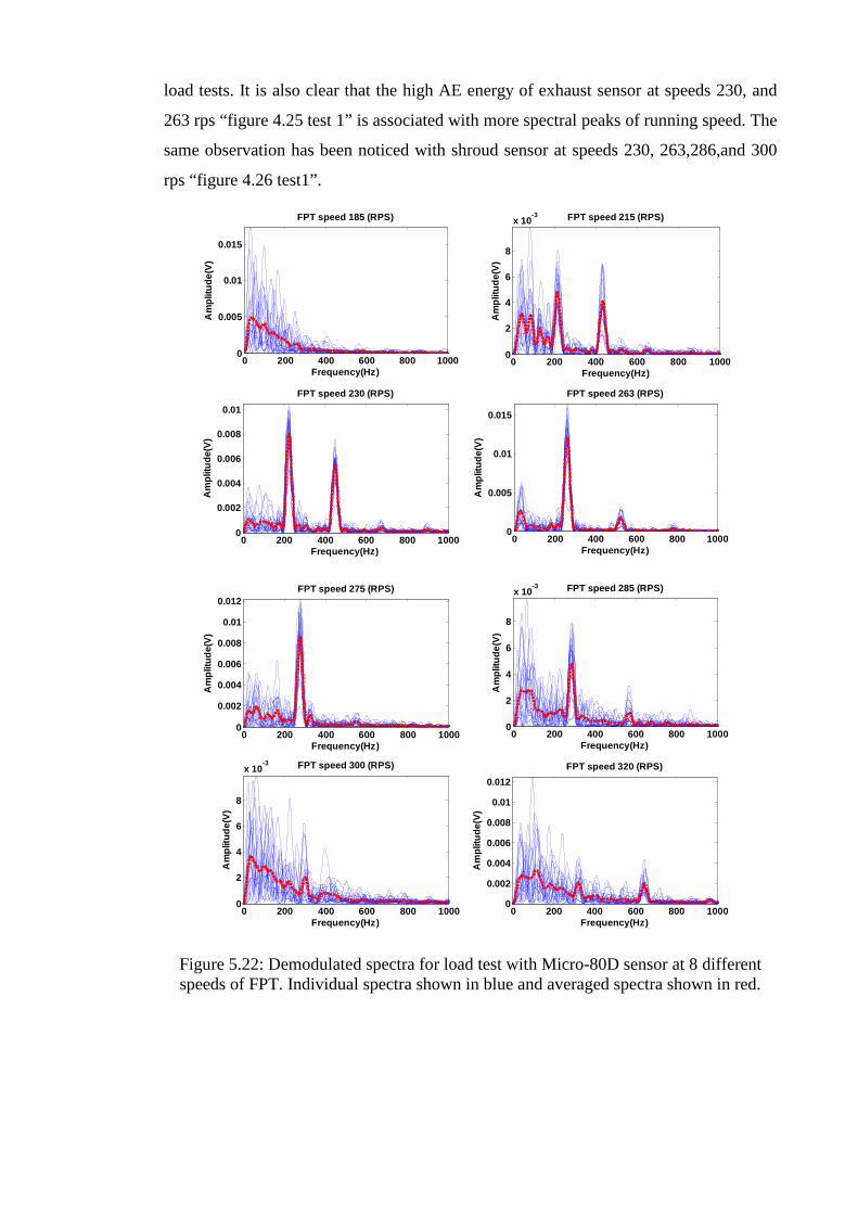
109
load tests. It is also clear that the high AE energy of exhaust sensor at speeds 230, and
263 rps “figure 4.25 test 1” is associated with more spectral peaks of running speed. The
same observation has been noticed with shroud sensor at speeds 230, 263,286,and 300
rps “figure 4.26 test1”.
0 200 400 600 800 10000
0.005
0.01
0.015
Frequency(Hz)
Am
plit
ud
e(V
)FPT speed 185 (RPS)
0 200 400 600 800 10000
2
4
6
8
x 10-3
Frequency(Hz)
Am
plit
ud
e(V
)
FPT speed 215 (RPS)
0 200 400 600 800 10000
0.002
0.004
0.006
0.008
0.01
Frequency(Hz)
Am
plit
ud
e(V
)
FPT speed 230 (RPS)
0 200 400 600 800 10000
0.005
0.01
0.015
Frequency(Hz)
Am
plit
ud
e(V
)
FPT speed 263 (RPS)
0 200 400 600 800 10000
0.002
0.004
0.006
0.008
0.01
0.012
Frequency(Hz)
Am
plit
ud
e(V
)
FPT speed 275 (RPS)
0 200 400 600 800 10000
2
4
6
8
x 10-3
Frequency(Hz)
Am
plit
ud
e(V
)
FPT speed 285 (RPS)
0 200 400 600 800 10000
2
4
6
8
x 10-3
Frequency(Hz)
Am
plit
ud
e(V
)
FPT speed 300 (RPS)
0 200 400 600 800 10000
0.002
0.004
0.006
0.008
0.01
0.012
Frequency(Hz)
Am
plit
ud
e(V
)
FPT speed 320 (RPS)
Figure 5.22: Demodulated spectra for load test with Micro-80D sensor at 8 different speeds of FPT. Individual spectra shown in blue and averaged spectra shown in red.

110
0 200 400 600 800 10000
1
2
3
4
5
x 10-3
Frequency (Hz)
Am
plit
ud
e(V
)
FPT speed 185 (RPS)
0 200 400 600 800 10000
2
4
6
8x 10
-3
Frequency (Hz)
Am
plit
ud
e(V
)
FPT speed 215 (RPS)
0 200 400 600 800 10000
0.002
0.004
0.006
0.008
0.01
0.012
Frequency (Hz)
Am
plit
ud
e(V
)
FPT speed 225 (RPS)
0 200 400 600 800 10000
0.002
0.004
0.006
0.008
0.01
Frequency (Hz)
Am
plit
ud
e(V
)
FPT speed 263 (RPS)
0 200 400 600 800 10000
0.005
0.01
0.015
Frequency (Hz)
Am
plit
ud
e(V
)
FPT speed 275 (RPS)
0 200 400 600 800 10000
0.02
0.04
0.06
0.08
0.1
Frequency (Hz)
Am
plit
ud
e(V
)FPT speed 285 (RPS)
0 200 400 600 800 10000
2
4
6
8
x 10-3
Frequency (Hz)
Am
plit
ud
e(V
)
FPT speed 300 (RPS)
0 200 400 600 800 10000
1
2
3
4
5
6
x 10-3
Frequency (Hz)
Am
plit
ud
e(V
)
FPT speed 320 (RPS)
Figure 5.23: Demodulated spectra for load test with S9215 sensor at 8 different speeds
of FPT. Individual spectra shown in blue and averaged spectra shown in red.
5.2.3. Demodulated frequency domain feature classification
To provide a complementary analysis to that presented in section 5.1.2, a set of features
were generated from the demodulated frequency analysis as input to an ANN with the
same specification as for the analysis based on time features. The features were
selected to employ as much of the information seen in Figures 5.20 to 5.23 as possible
without the computational burden of using the entire spectrum as input to the ANN.
Across the 20 records at each speed in each experiment the ten highest amplitude

111
frequencies were first identified and the energies and the frequencies of the five
commonest frequencies used as input to the ANN. As before, half of the data set was
used to train the network to the measured running speed and the network was then
tested, delivering weights to the output nodes from which a speed classification and an
estimate of running speed could be obtained. Figure 5.24 shows the ANN classification
performance to be superior to that using time-based features (Figure 5.10) with
classification being better than 90% for all individual tests and over 80% for the
grouped data. Figures 5.25 to 5.28 show the ANN speed error which, compared with the
time-based assessment, exhibits a very high level of certainty for most of the
classifications, the performance of the Micro-80D sensor being generally better than the
S2910. The relatively poor performance on the grouped data for the S92105 sensor on
the load tests can be seen to be confined to a few records where the speed estimate is
well away from the actual.
Test 1 Test 2 Test 3 All Tests0
10
30
50
70
90
(a)
AN
N P
erfo
rman
ce(%
)
Test 1 Test 2 Test 3 All Tests0
10
30
50
70
90
(b)
AN
N P
erfo
rman
ce(%
)
Test 1 Test 2 Test 3 All Tests0
10
30
50
70
90
(c)
AN
N P
erfo
rman
ce(%
)
Test 1 Test 2 Test 3 All Tests0
10
30
50
70
90
(d)
AN
N P
erfo
rman
ce(%
)
Figure 5. 24: (a) S9215 without load tests, (b) Micro-80D sensor without load tests, (c) S9215 sensor with load tests, (d) Micro-80D sensor with load tests.

112
0 20 40 60 80 100150
200
250
300
350
Record number
Sp
ee
d(R
PS
)
Test 1
0 50 100 150100
150
200
250
300
350
Record number
Sp
ee
d(R
PS
)
Test 2
0 50 100 150150
200
250
300
350
Record number
Sp
ee
d(R
PS
)
Test 3
0 100 200 300 400100
150
200
250
300
350
400
Record number
Sp
ee
d(R
PS
)
All Tests
ANN speed
Real speed
ANN speed
Real speed
ANN speed
Real speed
ANN speed
Real speed
Figure 5.25: ANN speed estimate error for S9215 sensor on idling test.
0 20 40 60 80 100150
200
250
300
350
Record number
Sp
ee
d(R
PS
)
Test 1
0 50 100 150100
150
200
250
300
350
Record number
Sp
ee
d(R
PS
)
Test 2
0 50 100 150150
200
250
300
350
400
Record number
Sp
ee
d(R
PS
)
Test 3
0 100 200 300 400100
150
200
250
300
350
400All tests
Record number
Sp
ee
d(R
PS
)
ANN speed
Real speed
ANN speed
Real speed
ANN speed
Real speed
ANN speed
Real speed
Figure 5.26: ANN speed estimate error for Micro-80D sensor on idling test.

113
0 20 40 60 80 100150
200
250
300
350
400
Record number
Sp
eed
(RP
S)
Test 1
0 20 40 60 80 100150
200
250
300
350
400
Record number
Sp
eed
(RP
S)
Test 2
0 20 40 60 80 100100
150
200
250
300
350
400
Record number
Sp
eed
(RP
S)
Test 3
0 50 100 150 200 250 300100
150
200
250
300
350
400
Record number
Sp
eed
(RP
S)
All test
ANN speedReal speed
ANN speedReal speed
ANN speed
Real speed
ANN speed
Real speed
Figure 5.27 : ANN speed estimate error for S9215 sensor on load test.
0 20 40 60 80 100150
200
250
300
350
400
Record number
Sp
eed
(RP
S)
Test 1
0 20 40 60 80 100150
200
250
300
350
400
Record number
Sp
eed
(RP
S)
Test 2
0 20 40 60 80 100100
150
200
250
300
350
400
Record number
Sp
eed
(RP
S)
Test 3
0 50 100 150 200 250 300100
150
200
250
300
350
400
Record number
Sp
eed
(RP
S)
All tests
ANN speed
Real speed
ANN speed
Real speed
ANN speed
Real speed
ANN speed
Real speed
Figure 5.28: ANN speed estimate error for Micro-80D sensor on load test.

114
5.3. Analysis combining time features and demodulated
frequency features
Because it relies on the energy of the signal, the statistical time-based analysis suffers
from two potential drawbacks. Firstly, calibration of the sensors is required on every
application as the energy will depend on many factors not related to the running
condition, not the least of them being the source-sensor distance and the quality of the
coupling. Secondly, the statistical time-based ANN is probably doing little more than a
multi-point fit to curves such as in figure 4.25, and this is why it is susceptible to
changes in the positions of peaks in the repeat tests. On the other hand, although the
frequency-based analysis can clearly identify instabilities in the same evolutions, it is
not able to detect the clear (albeit weaker) trends in stable regimes, such as that shown
in figure 4.10.
Therefore, this section seeks to combine the strengths of the time-based analysis with
the frequency-based analysis to obtain a better understanding of the sources of AE in the
tests and how these might be used to produce a model for normal running of the turbine.
5.3.1. Pulse shape recognition combined with frequency features
The pulse shape recognition network, although it shows poor performance, has the
potential advantage over the statistical one in that it is not amplitude-dependent and the
pulse-space approach also encodes some non-periodic frequency information. Figure
5.29 shows the effect of combining the pulse shape recognitions with raw AE features
and, clearly, the performance is only marginally better than the pulse shape recognition
alone, and poorer than the raw AE feature performance. The pulse-space approach
achieves its best performance when it is combined with demodulated frequency
approach to perform up to 90% for both sensors (figure 5.30).
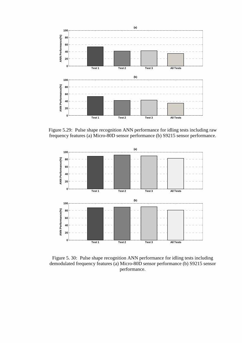
115
Test 1 Test 2 Test 3 All Tests0
20
40
60
80
100
AN
N P
erfo
rman
ce(%
)
(a)
Test 1 Test 2 Test 3 All Tests0
20
40
60
80
100
AN
N P
erfo
rman
ce(%
)
(b)
Figure 5.29: Pulse shape recognition ANN performance for idling tests including raw frequency features (a) Micro-80D sensor performance (b) S9215 sensor performance.
Test 1 Test 2 Test 3 All Tests0
20
40
60
80
100
AN
N P
erfo
rman
ce(%
)
(a)
Test 1 Test 2 Test 3 All Tests0
20
40
60
80
100(b)
AN
N P
erfo
rman
ce(%
)
Figure 5. 30: Pulse shape recognition ANN performance for idling tests including
demodulated frequency features (a) Micro-80D sensor performance (b) S9215 sensor performance.
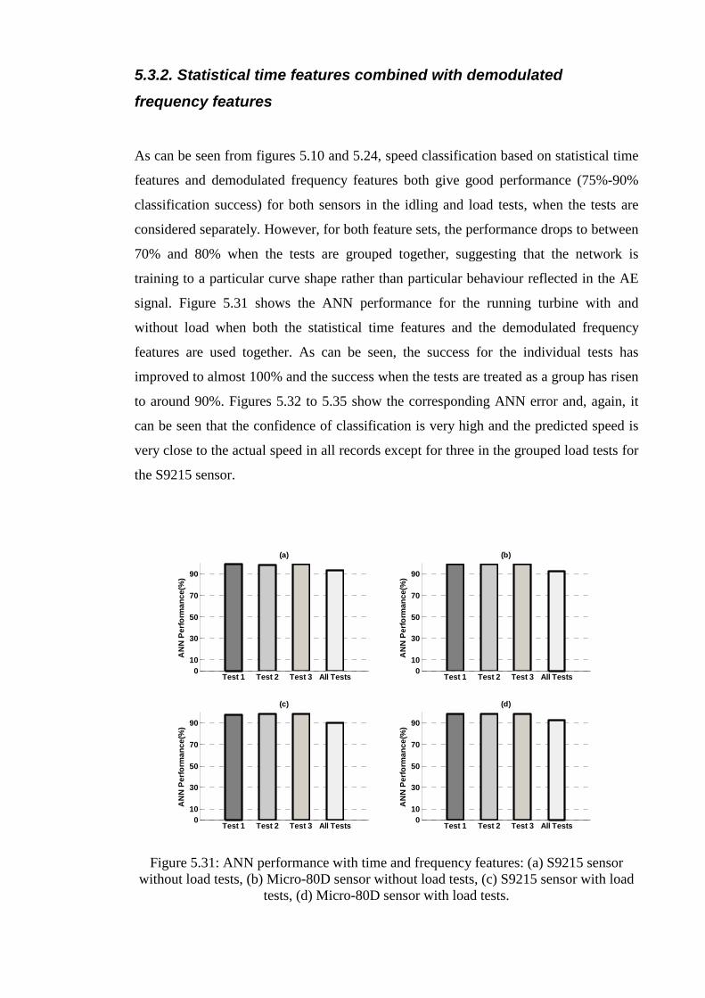
116
5.3.2. Statistical time features combined with demodulated
frequency features
As can be seen from figures 5.10 and 5.24, speed classification based on statistical time
features and demodulated frequency features both give good performance (75%-90%
classification success) for both sensors in the idling and load tests, when the tests are
considered separately. However, for both feature sets, the performance drops to between
70% and 80% when the tests are grouped together, suggesting that the network is
training to a particular curve shape rather than particular behaviour reflected in the AE
signal. Figure 5.31 shows the ANN performance for the running turbine with and
without load when both the statistical time features and the demodulated frequency
features are used together. As can be seen, the success for the individual tests has
improved to almost 100% and the success when the tests are treated as a group has risen
to around 90%. Figures 5.32 to 5.35 show the corresponding ANN error and, again, it
can be seen that the confidence of classification is very high and the predicted speed is
very close to the actual speed in all records except for three in the grouped load tests for
the S9215 sensor.
Test 1 Test 2 Test 3 All Tests0
10
30
50
70
90
(a)
AN
N P
erfo
rman
ce(%
)
Test 1 Test 2 Test 3 All Tests0
10
30
50
70
90
(b)
AN
N P
erfo
rman
ce(%
)
Test 1 Test 2 Test 3 All Tests0
10
30
50
70
90
(c)
AN
N P
erfo
rman
ce(%
)
Test 1 Test 2 Test 3 All Tests0
10
30
50
70
90
(d)
AN
N P
erfo
rman
ce(%
)
Figure 5.31: ANN performance with time and frequency features: (a) S9215 sensor
without load tests, (b) Micro-80D sensor without load tests, (c) S9215 sensor with load tests, (d) Micro-80D sensor with load tests.

117
0 20 40 60 80 100150
200
250
300
350
Record number
Sp
eed
(RP
S)
Test 1
0 50 100 150100
150
200
250
300
350
Record number
Sp
eed
(RP
S)
Test 2
0 50 100 150150
200
250
300
350Test 3
Record number
Sp
eed
(RP
S)
0 100 200 300 400100
150
200
250
300
350
Record number
Sp
eed
(RP
S)
All tests
ANN speedReal speed
ANN speedReal speed
ANN speedReal speed
ANN speedReal speed
Figure 5.32: ANN error for S9215 sensor during without load test.
0 20 40 60 80 100150
200
250
300
350Test 1
Record number
Sp
eed
(RP
S)
0 50 100 150100
150
200
250
300
350
Record number
Sp
eed
(RP
S)
Test 2
0 50 100 150150
200
250
300
350
Record number
Sp
eed
(RP
S)
Test 3
0 100 200 300 400100
150
200
250
300
350
Record number
Sp
eed
(RP
S)
All tests
ANN speed
Real speed
ANN speed
Real speed
ANN speedReal speed
ANN speedReal speed
Figure 5.33: ANN error for Micro-80D sensor during without load test.

118
0 20 40 60 80 100150
200
250
300
350
400
Record number
Sp
eed
(RP
S)
Test 1
0 20 40 60 80 100150
200
250
300
350Test 2
Record number
Sp
eed
(RP
S)
0 20 40 60 80 100100
150
200
250
300
350
400
Record number
Sp
eed
(RP
S)
Test 3
0 50 100 150 200 250 300100
150
200
250
300
350
400
Record number
Sp
eed
(RP
S)
All tests
ANN speed
Real speed
ANN speed
Real speed
ANN speed
Real speed
ANN speed
Real speed
Figure 5.34: ANN error for S9215 sensor during with load test.
0 20 40 60 80 100150
200
250
300
350
400
Record number
Spe
ed(R
PS
)
Test 1
0 20 40 60 80 100150
200
250
300
350
Record number
Spe
ed(R
PS
)Test 2
0 20 40 60 80 100100
150
200
250
300
350
400
Record number
Spe
ed(R
PS
)
Test 3
0 50 100 150 200 250 300100
150
200
250
300
350
400
Record number
Spe
ed(R
PS
)
All test
ANN speedReal speed
ANN speedReal speed
ANN speedReal speed
ANN speedReal speed
Figure 5.35: ANN error for Micro-80D sensor during with load test.

119
5.4. Discussion of AE sources in the running turbine
Chapter 4 illustrated that the AE generated in a gas turbine has two components; a
background broad band source, probably due to the turbulent gas flow through various
parts of the turbine, plus some peaks whose speed position varies a bit between tests,
and which are associated with peaks in the demodulated frequency spectrum.
The background AE energy increases smoothly with speed and, on the basis of other
work on flow in confined spaces in machinery, it would be expected that the energy of
such a source would depend on the nature of the fluid, the flow rate and the size(s) of
any orifice(s) in the flow [124, 125]. Also, it would be expected that such sources, if
localized, would be able to be traced to certain zones within the machine [17, 126].
The analysis in Chapter 5 has shown that this background energy associated with gas
flow begins to become modulated when the impeller is rotating and, at higher speeds,
there are a number of spectral peaks in the 20-1000Hz range. These spectral peaks
disrupt the smooth evolution of energy vs running speed and the peaks in the energy
curve, as well as the speed at which certain spectral peaks appear, are not precisely
reproducible in repeat tests. However, as shown by the ANN analysis, the behavior of
the turbine can be characterized by a combination of the energy within those spectral
peaks bands and the overall energy. Potential sources of the spectral peaks are; the
combustion chamber, the impeller, the exhaust, and feedback between the alternator and
the impeller under load. For the same running speed, the AE signature for the loaded
and idling conditions is different and, for the same test, the behaviour recorded at the
exhaust-mounted and shroud-mounted sensors is different. This section is devoted to
trying to understand these patterns in terms of the sources of AE within the turbine.
The first stage is to separate the two components of the signal in a systematic way. The
“spectral peaks energy” in each record, identified as the total energy in the five highest
peaks of the demodulated frequency spectrum (which typically accounts for 80% of
spectral peaks energy) was subtracted from the total energy to leave the background.
Figures 5.36 to 5.38 show the spectral peaks energy removal for each of the repeats of
each of the tests. In each figure, the black curves in the first three graphs show the best
exponential fit to the energy after removing the spectral peaks energy for each repeat
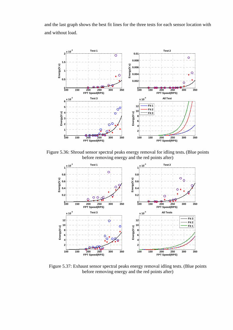
120
and the last graph shows the best fit lines for the three tests for each sensor location with
and without load.
100 150 200 250 300 3500
0.5
1
1.5
2x 10
-3
FPT Speed(RPS)
En
erg
y(V
.s)
Test 1
100 150 200 250 300 3500
0.002
0.004
0.006
0.008
0.01
FPT Speed(RPS)
En
erg
y(V
.s)
Test 2
100 150 200 250 300 3500
1
2
3
4
5
6x 10
-3
FPT Speed(RPS)
En
erg
y(V
.s)
Test 3
100 150 200 250 300 350
2
4
6
8
10
12
x 10-4
FPT Speed(RPS)
En
erg
y(V
.s)
All Test
Fit 1
Fit 2Fit 3
Figure 5.36: Shroud sensor spectral peaks energy removal for idling tests. (Blue points before removing energy and the red points after)
100 150 200 250 300 3500
0.2
0.4
0.6
0.8
1x 10
-3
FPT Speed(RPS)
En
erg
y(V
.s)
Test 1
100 150 200 250 300 3500
0.2
0.4
0.6
0.8
1x 10
-3
FPT Speed(RPS)
En
erg
y(V
.s)
Test 2
100 150 200 250 300 350
2
4
6
8
10
12
x 10-4
FPT Speed(RPS)
En
erg
y(V
.s)
Test 3
100 150 200 250 300 350
2
4
6
8
10
12
x 10-4
FPT Speed(RPS)
En
erg
y(V
.s)
All Tests
Fit 3
Fit 2Fit 1
Figure 5.37: Exhaust sensor spectral peaks energy removal idling tests. (Blue points before removing energy and the red points after)

121
100 150 200 250 300 350 4000
0.005
0.01
0.015
0.02
FPT Speed(RPS)
En
erg
y(V
.s)
Test 1
100 150 200 250 300 350 4000
0.01
0.02
0.03
0.04
0.05
FPT Speed(RPS)
En
erg
y(V
.s)
Test 2
100 150 200 250 300 350 4000
0.005
0.01
0.015
0.02
0.025
0.03
FPT Speed(RPS)
En
erg
y(V
.s)
Test 3
100 150 200 250 300 350 400
0.005
0.01
0.015
0.02
0.025
FPT Speed(RPS)
En
erg
y(V
.s)
All Tests
Fit 1
Fit 2 Fit 3
Figure 5.38: Shroud sensor spectral peaks removal load tests. (Blue points before removing energy and the red points after)
100 150 200 250 300 350 4000
0.1
0.2
0.3
0.4
0.5
0.6
FPT Speed(RPS)
En
erg
y(V
.s)
Test 1
100 150 200 250 300 350 4000
0.05
0.1
0.15
0.2
0.25
0.3
FPT Speed(RPS)
En
erg
y(V
.s)
Test 2
100 150 200 250 300 350 4000
0.005
0.01
0.015
0.02
FPT Speed(RPS)
En
erg
y(V
.s)
Test 3
100 150 200 250 300 350 400
0.005
0.01
0.015
0.02
0.025
FPT Speed(RPS)
En
erg
y(V
.s)
All Tests
Fit 1
Fit 2 Fit 3
Figure 5.39: Exhaust sensor spectral peaks removal load tests. (Blue points before removing energy and the red points after)
The background AE energy thus obtained from the idling test is compared with the
background energy for the static impeller tests (jammed impeller, without impeller) in
Figures 5.40 and 5.41, re-plotted against the combustion gas flow rate through the
turbine. It is clear that the AE energy is mainly correlated with gas flow resistance,
where it is lowest for the test without an impeller where the resistance to gas flow
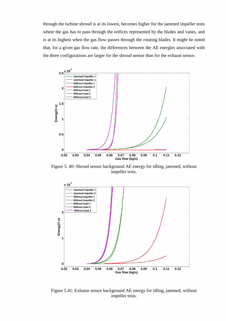
122
through the turbine shroud is at its lowest, becomes higher for the jammed impeller tests
where the gas has to pass through the orifices represented by the blades and vanes, and
is at its highest when the gas flow passes through the rotating blades. It might be noted
that, for a given gas flow rate, the differences between the AE energies associated with
the three configurations are larger for the shroud sensor than for the exhaust sensor.
0.02 0.03 0.04 0.05 0.06 0.07 0.08 0.09 0.1 0.11 0.12
0
0.5
1
1.5
2
2.5x 10
-3
Gas flow (kg/s)
En
erg
y(V
.s)
Jammed impeller 1Jammed impeller 1Without impeller 1Without impeller 2Without load 1Without load 2Without load 3
Figure 5. 40: Shroud sensor background AE energy for idling, jammed, without
impeller tests.
0.02 0.03 0.04 0.05 0.06 0.07 0.08 0.09 0.1 0.11 0.12
0
1
2
x 10-4
Gas flow (kg/s)
En
erg
y(V
.s)
Jammed impeller 1Jammed impeller 2Without impeller 1Without impeller 2Without load 1Without load 2 Without load 3
Figure 5.41: Exhaust sensor background AE energy for idling, jammed, without impeller tests.

123
The background AE energy for the idling test is compared with the background energy
for the load test in Figures 5.42 and 5.43, in this case plotted against free power turbine
speed. At a given speed, the load test contains more background AE energy only for the
exhaust sensor; for the shroud sensor the background is, if anything higher for the idling
test. At a given FPT speed, this suggests that loading results in a reduced background
flow noise associated with the blades, and an increased flow noise associated with the
exhaust.
100 200 300 400 500 600 700 800 900 10000
0.05
0.1
0.15
0.2
0.25
Free power turbine speed(RPS)
En
erg
y(V
.s)
With load 1With load 2With load 3Without load 1Without load 2Without load 3
Figure 5.42: Shroud sensor background AE energy for idling and load tests.
100 200 300 400 500 600 700 800 900 10000
0.1
0.2
0.3
0.4
0.5
0.6
0.7
0.8
0.9
1
Free power turbine speed(RPS)
En
erg
y(V
.s)
Without load 1Without load 2Without load 3With load 1With load 2With load 3
Figure 5.43: Exhaust sensor background AE energy for idling and load tests.
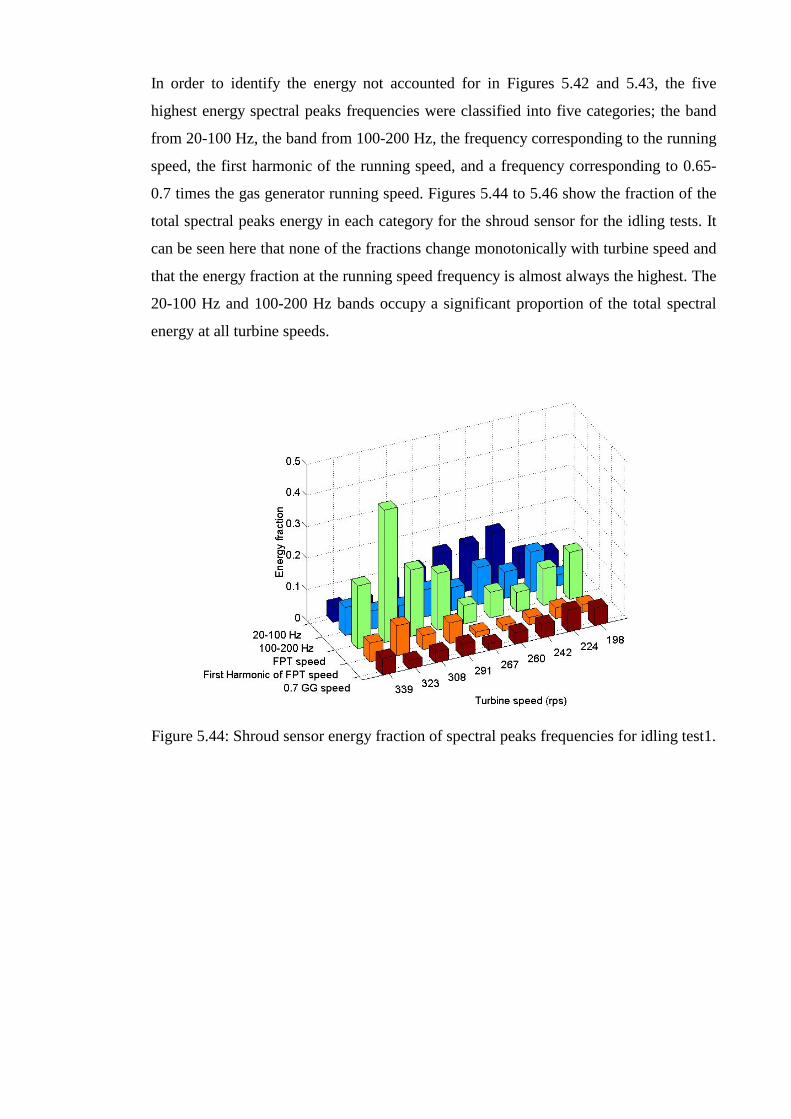
124
In order to identify the energy not accounted for in Figures 5.42 and 5.43, the five
highest energy spectral peaks frequencies were classified into five categories; the band
from 20-100 Hz, the band from 100-200 Hz, the frequency corresponding to the running
speed, the first harmonic of the running speed, and a frequency corresponding to 0.65-
0.7 times the gas generator running speed. Figures 5.44 to 5.46 show the fraction of the
total spectral peaks energy in each category for the shroud sensor for the idling tests. It
can be seen here that none of the fractions change monotonically with turbine speed and
that the energy fraction at the running speed frequency is almost always the highest. The
20-100 Hz and 100-200 Hz bands occupy a significant proportion of the total spectral
energy at all turbine speeds.
Figure 5.44: Shroud sensor energy fraction of spectral peaks frequencies for idling test1.

125
Figure 5.45: Shroud sensor energy fraction of spectral peaks frequencies of idling test2.
Figure 5.46: Shroud sensor energy fraction of spectral peaks frequencies of idling test3.

126
Figures 5.47 to 5.49 show the energy fractions for the exhaust sensor for the idling tests.
The running speed frequency still has the highest proportion of spectral energy at all
turbine speeds and the 20-100 Hz and 100-200 Hz bands seem to be higher than those
for the shroud sensor for idling tests. 0.7 GG frequency has higher proportion of energy
at lower speed of gas turbine than that of higher turbine speeds.
Figure 5.47: Exhaust sensor energy fraction of spectral peaks frequencies of idling test1.
Figure 5.48: Exhaust sensor energy fraction of spectral peaks frequencies of idling test2.

127
Figure 5.49: Exhaust sensor energy fraction of spectral peaks frequencies of idling test3.
Figure 5.50 to 5.55 show the energy fraction of spectral peaks frequencies of both
shroud and exhaust sensors for the load tests. The observations are similar to those
for the idling tests for both sensors with the running speed frequency having the
highest energy proportion and the 20 -100 Hz and 100-200 Hz bands being stronger
and higher with the exhaust sensor than the shroud sensor. In the load tests the
running speed frequency and its harmonics are generally stronger than that in the
idling tests for both sensors and the 0.7 GG frequency is absent amongst the five
highest energy bands.
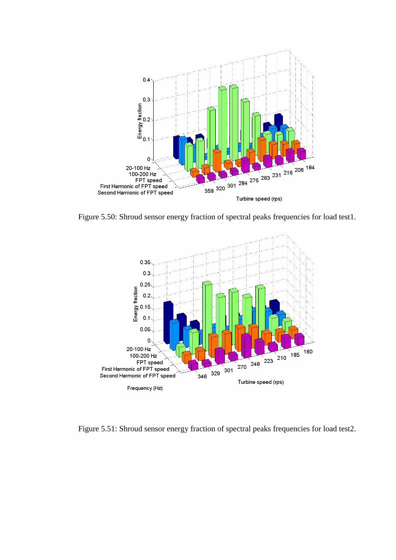
128
Figure 5.50: Shroud sensor energy fraction of spectral peaks frequencies for load test1.
Figure 5.51: Shroud sensor energy fraction of spectral peaks frequencies for load test2.
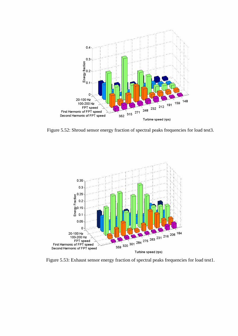
129
Figure 5.52: Shroud sensor energy fraction of spectral peaks frequencies for load test3.
Figure 5.53: Exhaust sensor energy fraction of spectral peaks frequencies for load test1.

130
Figure 5.54: Exhaust sensor energy fraction of spectral peaks frequencies for load test2.
Figure 5.55: Exhaust sensor energy fraction of spectral peaks frequencies for load test3.

131
Figure 5.56: Schematic of gas turbine exhaust system.
Figure 5.56 shows a schematic diagram of the turbine exhaust, which consists of two
pipes of 100 mm and 300 mm diameter and length1.69 m and 4.15 m, respectively. The
temperature of the exhaust gases varies between 400 and 530°C for the load and idling
tests, respectively, and the speed of sound, c (ms-1), in each tube can be calculated from:
M
RTc
g= (5.1)
where
γ is the adiabatic index of the gas
R is the molar gas constant (Jmol−1K−1).
T is the absolute temperature (K)
M is the molar mass (kgmol−1)
The reverberation frequency, f (Hz), in the tube can be estimated from:
NLc
f2
= (5.2)
where
N = 1,2,3,…..
L is the length of the tube (m)
From equation 5.2 the reverberation frequency in the smaller diameter pipe can be
estimated to be between 100 and 200 Hz, and, in the larger diameter pipe between 20

132
and 100 Hz. This suggests that the energy in the 20-100 Hz and 100-200 Hz bands are
associated with exhaust reverberations and explains why these are expressed more
strongly in the exhaust sensor than the shroud sensor for both load and idling tests.
For the idling tests, the running speed frequency and its harmonics seem to be more
strongly expressed at specific turbine speeds and examination of these speeds has
shown them to be coincident with the first harmonic of the reverberation frequency of
the small diameter exhaust pipe, suggesting that the reverberation frequency is powering
the running speed frequency in the turbine. On the other hand the higher energy
associated with the running speed frequency and its harmonics in the load tests indicates
that the spectral peaks here are dominated by feedback between the turbine impeller and
alternator. Table 5.1 and table 5.2 show running speeds, exhaust temperatures, and
reverberation frequencies of exhaust1 and exhaust 2.
Idling test Turbine speed
(RPS) Exhaust
temperature(C0) Exhaust sound speed (m/s)
Exhaust1 frequency(HZ)
Exhaust2 frequency(HZ)
190 420 521 156.0 63.5 206 430 525 157.1 64.0 220 435 526 157.6 64.2 231 440 528 158.1 64.4 241 445 530 158.6 64.6 250 450 530 158.6 64.6 256 455 531 159.1 64.8 265 460 535 160.2 65.2 275 465 535 160.2 65.2 284 470 535 160.1 65.2 294 475 537 160.7 65.4 308 480 537 160.6 65.4 321 485 538 161.2 65.6 333 495 538 161.2 65.6 342 505 541 162.1 66.0
Table 5. 1: Thermo features of idling test.

133
Load test Turbine speed
(RPS) Exhaust
temperature(C0) Exhaust sound speed (m/s)
Exhaust1 frequency(HZ)
Exhaust2 frequency(HZ)
184 520 555 164.1 66.8 206 520 555 164.1 66.8 216 520 555 164.1 66.8 231 520 555 164.1 66.8 263 520 555 164.1 66.8 275 520 555 164.1 66.8 284 520 555 164.1 66.8 301 520 555 164.1 66.8 320 520 555 164.1 66.8 359 520 555 164.1 66.8
Table 5. 2: Thermo features of load test.

134
Chapter 6: Faulty impeller condition monitoring tests This chapter describes, analyses and discusses the results of the tests carried out on the
turbine with an impeller which had been damaged by removal of the tips of some of the
vanes. The tests were carried out with the same sensor positioning as the load tests
whose results were described in chapter 4 and analysed in chapter 5. The defective
impeller tests were also carried out in the same way, i.e. the speed being varied by gas
and air flow.
The results are first described for each of the degrees of damage (two damaged blades
and four damaged blades) in comparison with the tests with undamaged blades. Finally
the results are analysed against the background of the findings of chapter 5 to assess
how impeller damage in the FPT can be detected against the already complex pattern of
AE generated in normal operation.
6.1. Results of tests with two damaged blades
Figures 6.1 to 6.9 show the results in a form that can be compared to figures 4.16-4.22.
Figures 6.1 and 6.2 show samples of scaled AE signals from the two sensors at nine
different speeds of the FPT along the corresponding signal envelopes. Compared with
the corresponding examples in figures 4.16 and 4.17 these signals show a much higher
density of sharp rise-time pulses, especially for the shroud-mounted sensor, indicating a
significant effect in the FPT. The most striking difference, however, is that the signal
recorded at the shroud becomes distinctly periodic at higher speeds.

135
0 0.005 0.01 0.015 0.02 0.025 0.03S1
S2
S3
S4
S5
S6
S7
S8
S9
Time(Sec)
No
rmal
ized
Am
plit
ud
e(A
rbitr
ary
un
it)
Figure 6.1: Typical Micro-80D AE signatures (exhaust) for test with two damaged blades. Free power turbine speed increases from bottom to top, with S1 recorded at 95
RPS and S9 recorded at 325 RPS.
0 0.005 0.01 0.015 0.02 0.025 0.03S1
S2
S3
S4
S5
S6
S7
S8
S9
Time(Sec)
No
rmal
ized
Am
plit
ud
e(A
rbitr
ary
un
it)
Figure 6.2: Typical S9215 AE signatures (shroud) for test with two damaged blades. Free power turbine speed increases from bottom to top, with S1 recorded at 95 RPS and
S9 recorded at 325 RPS.
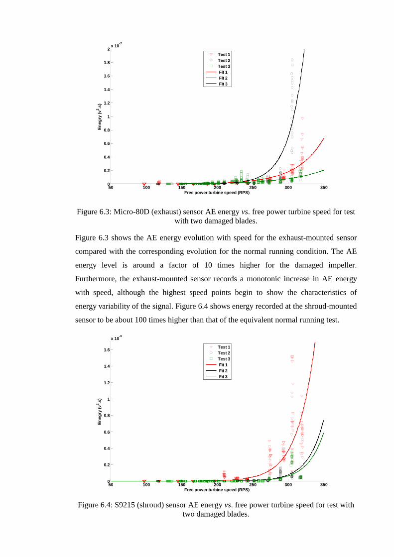
136
50 100 150 200 250 300 3500
0.2
0.4
0.6
0.8
1
1.2
1.4
1.6
1.8
2x 10
-7
Free power turbine speed (RPS)
En
egry
(v2.s
)
Test 1Test 2Test 3 Fit 1 Fit 2 Fit 3
Figure 6.3: Micro-80D (exhaust) sensor AE energy vs. free power turbine speed for test with two damaged blades.
Figure 6.3 shows the AE energy evolution with speed for the exhaust-mounted sensor
compared with the corresponding evolution for the normal running condition. The AE
energy level is around a factor of 10 times higher for the damaged impeller.
Furthermore, the exhaust-mounted sensor records a monotonic increase in AE energy
with speed, although the highest speed points begin to show the characteristics of
energy variability of the signal. Figure 6.4 shows energy recorded at the shroud-mounted
sensor to be about 100 times higher than that of the equivalent normal running test.
50 100 150 200 250 300 3500
0.2
0.4
0.6
0.8
1
1.2
1.4
1.6
x 10-6
Free power turbine speed (RPS)
En
egry
(v2.s
)
Test 1Test 2Test 3 Fit 1 Fit 2 Fit 3
Figure 6.4: S9215 (shroud) sensor AE energy vs. free power turbine speed for test with
two damaged blades.

137
Figure 6.5 shows raw AE spectra at nine different speeds for the impeller with two
damaged blades. Figure 6.5 (a) shows no change in the raw AE spectrum with running
speed for the exhaust-mounted sensor, not dissimilar to the situation for the normal
running condition. Also, there is little apparent difference between the normal condition
and condition with the defective impeller. For the shroud-mounted sensor, the main
30kHz activity reduces gradually in frequency as the speed increases, as is the case for
the undamaged impeller (Figure 4.20). There is a distinct change in the raw AE
spectrum at the two highest speeds, with some lower frequency (around 10-20kHz)
activity appearing, and some activity at around 50kHz at some intermediate speeds.
These secondary bands do not present in the normal running condition (Figure 4.20),
although in neither case is there a clear pattern associated with these frequencies. It
seems, therefore that the raw AE spectrum is not likely to be a strong indicator of
impeller damage.

138
0 0.5 1 1.5 2 2.5 3 3.5 4 4.5 5
x 105
S1
S2
S3
S4
S5
S6
S7
S8
S9
Frequency(Hz)
No
rmal
ized
vo
lt (
Arb
itra
ry u
nit
)
(a)
0 0.2 0.4 0.6 0.8 1 1.2 1.4 1.6 1.8 2
x 105
S1
S2
S3
S4
S5
S6
S7
S8
S9
Frequency(Hz)
No
rmal
ized
vo
lt (
Arb
itra
ry u
nit
)
(b)
Figure 6.5: Typical raw AE spectra for test with two damaged blades: (a) Micro-80D sensor, (b) S9215 sensor. Free power turbine speed increases from bottom to top, with
S1 recorded at 95 RPS and S9 recorded at 325 RPS. Figure 6.6 shows the demodulated frequency analysis for the exhaust-mounted sensor,
and these clearly lack the strong spectral peaks observed at low speed for the normal
running condition (Figure 5.20). At higher speeds, however, spectral peaks at multiples
of half the running speed begin to appear.

139
0 200 400 600 800 10000
0.002
0.004
0.006
0.008
0.01
0.012
Frequency(Hz)
Am
plit
ud
e(V
)
FPT speed(218 RPS)
0 200 400 600 800 10000
0.002
0.004
0.006
0.008
0.01
Frequency(Hz)
Am
plit
ud
e(V
)
FPT speed(227 RPS)
0 200 400 600 800 10000
0.002
0.004
0.006
0.008
0.01
0.012
Frequency(Hz)
Am
plit
ud
e(V
)
FPT speed(242 RPS)
0 200 400 600 800 10000
0.002
0.004
0.006
0.008
0.01
Frequency(Hz)
Am
plit
ud
e(V
)
FPT speed(267 RPS)
0 200 400 600 800 10000
0.002
0.004
0.006
0.008
0.01
0.012
Frequency(Hz)
Am
plit
ud
e(V
)
FPT speed(273 RPS)
0 200 400 600 800 10000
0.002
0.004
0.006
0.008
0.01
0.012
Frequency(Hz)
Am
plit
ud
e(V
)FPT speed(293 RPS)
0 200 400 600 800 10000
0.002
0.004
0.006
0.008
0.01
Frequency(Hz)
Am
plit
ud
e(V
)
FPT speed(305 RPS)
0 200 400 600 800 10000
0.002
0.004
0.006
0.008
0.01
Frequency(Hz)
Am
plit
ud
e(V
)
FPT speed(319 RPS)
Figure 6.6: Demodulated spectra for test with two damaged blades with Micro-80D sensor at 8 different speeds of FPT.

140
0 200 400 600 800 10000
1
2
3
4
5
6x 10
-3
Frequency(Hz)
Am
plit
ud
e(V
)
FPT speed(218 RPS)
0 200 400 600 800 10000
0.002
0.004
0.006
0.008
0.01
0.012
Frequency(Hz)
Am
plit
ud
e(V
)
FPT speed(242 RPS)
0 200 400 600 800 10000
0.002
0.004
0.006
0.008
0.01
Frequency(Hz)
Am
plit
ud
e(V
)
FPT speed(267 RPS)
0 200 400 600 800 10000
2
4
6
x 10-3
Frequency(Hz)
Am
plit
ud
e(V
)
FPT speed(227 RPS)
0 200 400 600 800 10000
2
4
6
x 10-3
Frequency(Hz)
Am
plit
ud
e(V
)
FPT speed(273 RPS)
0 200 400 600 800 10000
2
4
6
8
x 10-3
Frequency(Hz)
Am
plit
ud
e(V
)
FPT speed(293 RPS)
0 200 400 600 800 10000
2
4
6
x 10-3
Frequency(Hz)
Am
plit
ud
e(V
)
FPT speed(305 RPS)
0 200 400 600 800 10000
1
2
3
4
5x 10
-3
Frequency(Hz)
Am
plit
ud
e(V
)
FPT speed(319 RPS)
Figure 6.7 : Demodulated spectra for test with two damaged blades with S9215 sensor
at 8 different speeds of FPT. Figure 6.7 shows the demodulated frequency analysis of the shroud-mounted sensor. As
for the normal running condition (Figure 5.21), strong spectral peaks are present at the
running speed in many instances but, unlike the normal condition, very strong
harmonics of the running speed are present and, in some cases, harmonics at half the
running speeds are displayed.

141
6.2. Results of tests with four damaged blades Figures 6.8, 9, 10 and 11 to 6.13 show a summary of the energy and demodulated
frequency analyses for the test with four damaged blades and can be compared directly
with Figures 6.3, 6.4, 6.5 and 6.7.
0 0.005 0.01 0.015 0.02 0.025 0.03S1
S2
S3
S4
S5
S6
S7
S8
Time(Sec)
No
rmal
ized
Am
plit
ud
e(A
rbitr
ary
un
it)
Figure 6.8: Typical Micro-80D AE signatures (exhaust) for test with four damaged blades. Free power turbine speed increases from bottom to top, with S1 recorded at 110
RPS and S8 recorded at 385 RPS. Comparing figures 6.9 and 6.3 shows the AE energy recorded at the exhaust-mounted
sensor to be about a factor of two less than that of the test with two damaged blades.
The test with four damaged blades, however, shows variability in AE energy between
300 and 350 rps, which is absent in the test with two damaged blades. The shroud-
mounted sensor, on the other hand (Figure 6.10) records a rather similar level and
evolution of energy to the tests with two damaged blades (Figure 6.4).

142
100 150 200 250 300 350 4000
0.1
0.2
0.3
0.4
0.5
0.6
0.7
0.8
0.9
1x 10
-7
Free power turbine speed (RPS)
En
egry
(v2.s
)
Test 1Test 2Test 3 Fit 1 Fit 2 Fit 3
Figure 6.9: Micro-80D (exhaust) sensor AE energy vs. free power turbine speed for test
with four damaged blades.
100 150 200 250 300 350 4000
0.2
0.4
0.6
0.8
1
1.2
1.4
1.6
1.8
2x 10
-6
Free power turbine speed (RPS)
En
egry
(v2.s
)
Test 1Test 2Test 3 Fit 1 Fit 2 Fit 3
Figure 6.10: S9215 (shroud) sensor AE energy vs. free power turbine speed for test with four damaged blades.
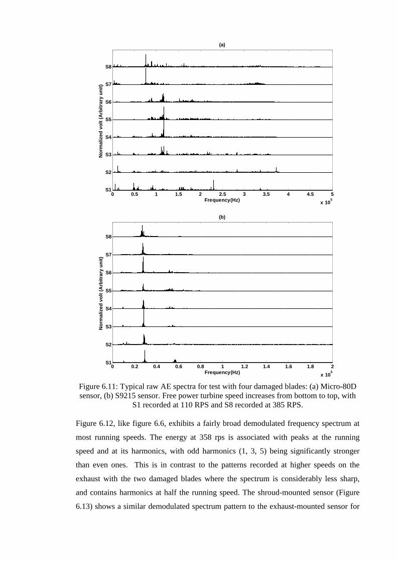
143
0 0.5 1 1.5 2 2.5 3 3.5 4 4.5 5
x 105
S1
S2
S3
S4
S5
S6
S7
S8
Frequency(Hz)
No
rmal
ized
vo
lt (
Arb
itra
ry u
nit
)
(a)
0 0.2 0.4 0.6 0.8 1 1.2 1.4 1.6 1.8 2
x 105
S1
S2
S3
S4
S5
S6
S7
S8
Frequency(Hz)
No
rmal
ized
vo
lt (
Arb
itra
ry u
nit
)
(b)
Figure 6.11: Typical raw AE spectra for test with four damaged blades: (a) Micro-80D sensor, (b) S9215 sensor. Free power turbine speed increases from bottom to top, with
S1 recorded at 110 RPS and S8 recorded at 385 RPS. Figure 6.12, like figure 6.6, exhibits a fairly broad demodulated frequency spectrum at
most running speeds. The energy at 358 rps is associated with peaks at the running
speed and at its harmonics, with odd harmonics (1, 3, 5) being significantly stronger
than even ones. This is in contrast to the patterns recorded at higher speeds on the
exhaust with the two damaged blades where the spectrum is considerably less sharp,
and contains harmonics at half the running speed. The shroud-mounted sensor (Figure
6.13) shows a similar demodulated spectrum pattern to the exhaust-mounted sensor for

144
the four damaged blades (Figure 6.12) and again contrasts with the equivalent for the
two damaged blades (Figure 6.7) in not exhibiting harmonics at half the running speed.
0 500 1000 1500 20000
0.005
0.01
Frequency(Hz)
Am
plit
ud
e(V
)
FPT speed(201 RPS)
0 500 1000 1500 20000
0.002
0.004
0.006
0.008
0.01
Frequency(Hz)
Am
plit
ud
e(V
)
FPT speed(221 RPS)
0 500 1000 1500 20000
2
4
6
8
x 10-3
Frequency(Hz)
Am
plit
ud
e(V
)
FPT speed(276 RPS)
0 500 1000 1500 20000
2
4
6
x 10-3
Frequency(Hz)
Am
plit
ud
e(V
)
FPT speed(312 RPS)
0 500 1000 1500 20000
0.002
0.004
0.006
0.008
0.01
0.012
Frequency(Hz)
Am
plit
ud
e(V
)
FPT speed(325 RPS)
0 500 1000 1500 20000
0.002
0.004
0.006
0.008
0.01
0.012
Frequency(Hz)
Am
plit
ud
e(V
)
FPT speed(335 RPS)
0 500 1000 1500 20000
2
4
6
x 10-3
Frequency(Hz)
Am
plit
ud
e(V
)
FPT speed(358 RPS)
0 500 1000 1500 20000
0.002
0.004
0.006
0.008
0.01
0.012
Frequency(Hz)
Am
plit
ud
e(V
)
FPT speed(386 RPS)
Figure 6.12: Demodulated spectra for test with four damaged blades with Micro-80D sensor at 8 different speeds of FPT.
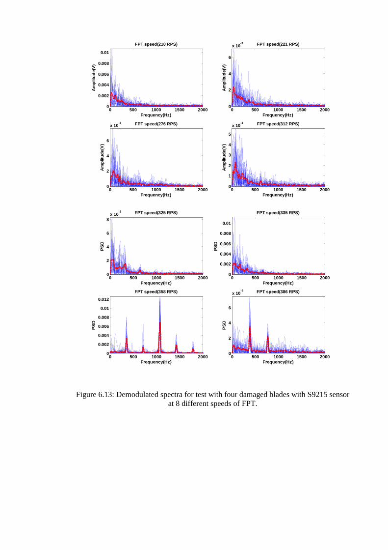
145
0 500 1000 1500 20000
0.002
0.004
0.006
0.008
0.01
Frequency(Hz)
Am
plit
ud
e(V
)
FPT speed(210 RPS)
0 500 1000 1500 20000
2
4
6
x 10-3
Frequency(Hz)
Am
plit
ud
e(V
)
FPT speed(221 RPS)
0 500 1000 1500 20000
2
4
6
x 10-3
Frequency(Hz)
Am
plit
ud
e(V
)
FPT speed(276 RPS)
0 500 1000 1500 20000
1
2
3
4
5
x 10-3
Frequency(Hz)
Am
plit
ud
e(V
)
FPT speed(312 RPS)
0 500 1000 1500 20000
2
4
6
8x 10
-3
Frequency(Hz)
PS
D
FPT speed(325 RPS)
0 500 1000 1500 20000
0.002
0.004
0.006
0.008
0.01
Frequency(Hz)
PS
DFPT speed(335 RPS)
0 500 1000 1500 20000
0.002
0.004
0.006
0.008
0.01
0.012
Frequency(Hz)
PS
D
FPT speed(358 RPS)
0 500 1000 1500 20000
2
4
6
x 10-3
Frequency(Hz)
PS
D
FPT speed(386 RPS)
Figure 6.13: Demodulated spectra for test with four damaged blades with S9215 sensor at 8 different speeds of FPT.

146
6.3. Discussion of damaged impeller tests
The previous sections confirm that damaged blades produce characteristic AE patterns
at some speeds, visible in the demodulated frequency domain. These patterns could
form the basis of a diagnostic system involving running the turbine through a range of
speeds to observe whether the pattern is excited. An example of such “tuning” can be
seen in figure 6.7, where, as the turbine speed goes towards the maximum of 320rps, the
spectral peaks pattern approaches its full expression. The corresponding effect occurs
over a narrower range of about 350rps for the impeller with four damaged blades.
Figure 6.14 shows an AE signature recorded on the shroud during the test where the
impeller has two damaged blades. The record has been chosen as one where the
characteristic spectral peaks are excited and, as well as the raw signal, the RMS
(averaging time of 0.03 ms) is shown along with the shaft encoder signal. As can be
seen, the time series exhibits a series of pulses, one per cycle, and the intensity of these
pulses alternates between cycles of the turbine. Figure 6.15 shows the corresponding
demodulated frequency analysis which exhibits two harmonic series, one at the running
speed and one at half the running speed. Such a pattern is typical of a train with two
unequally-sized, but symmetrically distributed, pulses per cycle Thakkar et al [127] and
the two-cycle repeat time of the pulse pair explains why a harmonic series at half the
running speed occurs.

147
0 0.005 0.01 0.015 0.02 0.025 0.03-2
-1.5
-1
-0.5
0
0.5
1
Time(sec)
Am
plit
de(
V)
S9215 signal at 319 RPS of FPTFPT Speed signalS9215 RMS Signal
Cycle
Figure 6. 14: AE signature recorded on shroud for test with two damaged blades.
0 500 1000 1500 2000 25000
0.5
1
1.5
2
2.5
3
3.5
4
4.5x 10
-3 FPT Speed 319 (RPS)
Frequency(Hz)
PS
D
Best fit of running speed peaksBest fit of half running speed peaksDemodulated frequency of S9215 signal
Figure 6.15: Demodulated frequency graph from shroud AE signature for test with two
damaged blades.

148
Figure 6.16 shows the AE signature of the impeller with four damaged blades, again at a
speed where the characteristic spectral peaks pattern is exhibited, but this time for the
exhaust-mounted sensor. Like the signal with two damaged blades the signal is
pulsatile, although this time there are two pulses per cycle and these are of
approximately the same height within and between cycles. Furthermore, the pulses are
unequally spaced. The pattern is also a little less clear than in figure 6.14. Figure 6.17
shows the corresponding demodulated frequency analysis with the dashed line tracing
the heights of the harmonics of the running speed, which can be seen to be roughly
sinusoidal in its shape. Again, such patterns are predictable Thakkar et al [127] and an
appropriate spectral analysis can therefore yield information on the pulse distribution.
0 0.005 0.01 0.015 0.02 0.025 0.03-0.8
-0.6
-0.4
-0.2
0
0.2
0.4
0.6
0.8
Time(sec)
Am
plit
de(
V)
Micro-80D signal at 355 RPS of FPTMicro-80D RMS SignalFPT Speed signal
cycle
Figure 6.16: AE signature recorded on exhaust for test with four damaged blades.
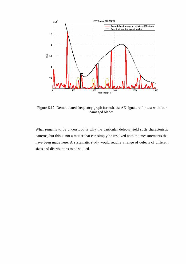
149
0 500 1000 1500 2000 2500
0.5
1
1.5
2
2.5
x 10-4
Frequency(Hz)
PS
D
FPT Speed 355 (RPS)
Demodulated frequency of Micro-80D signalBest fit of running speed peaks
Figure 6.17: Demodulated frequency graph for exhaust AE signature for test with four
damaged blades.
What remains to be understood is why the particular defects yield such characteristic
patterns, but this is not a matter that can simply be resolved with the measurements that
have been made here. A systematic study would require a range of defects of different
sizes and distributions to be studied.

150
Chapter 7 Conclusion and future work
In this work three types of experiments have been conducted, AE propagation and
calibration tests, AE monitoring of a healthy gas turbine under various operating
conditions, and AE diagnosis of a gas turbine with simulated impeller faults. The AE
propagation and calibration studies were essentially enabling tests to determine the
characteristics of AE propagation on the experimental gas turbine although they have
some generic value in assessing possible monitoring strategies for industrial scale
machines. The most significant contributions come from the understanding of how AE
is generated in gas turbines and how it might be used to monitor operating conditions
and detect blade faults. The main conclusions of the research are listed below, followed by
recommendations for future work.
7.1. Conclusions:
Sensor calibration:
1. The remounting and the repositioning of the AE sensors result in a variation in
the recorded AE energy for a pencil lead break source in a range of 10-45% and,
on a simple steel block, there is no other significant source of variation.
2. The turbine surface temperature affects the response of both AE sensors used;
the S9215 sensor on the turbine shroud is more sensitive at higher temperatures,
whereas the Micro-80D is less sensitive at higher temperatures.
3. Both of these findings have practical implications for sensor placement on
industrial turbines and, importantly, indicate that trending using amplitude-based
features will be difficult.
Propagation on gas turbine
1. In many parts of the machine, AE energy can be described as decaying
exponentially with increasing source-sensor distance.
2. Structural details and complications such as geometrical boundaries, webs, and
discontinuities have a considerable effect on the AE propagation causing a step
change in transmitted AE energy, attributed to leakage and reflection.
3. The AE energy in a field close to the source position (up to 0.04 m) has a high
variability due to the complex nature of near-field waves.

151
4. As expected, the shroud mounted sensor monitors AE emanating from the
turbine impeller better than the exhaust mounted sensor and vice versa.
Configuration tests:
1. The experiments without an impeller and with the jammed impeller
demonstrated a smooth evolution of AE energy with GGT speed. On the other
hand the experiments with a rotating impeller with and without load exhibited
complex AE energy against running speed and much higher levels of AE energy.
Thus the rotation of the turbine impeller has a significant influence on the AE
generated.
2. The general AE energy level increases with gas flow rate and with the
complexity of flow in turbine shroud, being lowest when the impeller is absent
and highest for the turbine running under load.
3. Whereas the AE energy level increases with turbine speed and can be curve-fit
reasonably reproducibly, this does not, in itself, provide an explanation for the
AE sources.
4. The AE records contain structural information such as pulses in the time series
and information in the frequency domain, but the patterns with running speed
are too complex to be elucidated by inspection.
Identification of operating condition in normal running.
1. Artificial neural networks can be used with time domain features to recognize
the complex AE pattern associated with gas turbine running speed. Using eight
time features the percentage of correct speed classification was 70-80%, and two
of the time features, the RMS and the standard deviation of the raw AE gave
performance at the 65-85% level on their own.
2. Artificial neural network performance using only demodulated frequency
features was better than that of the time features alone, but the combination of
frequency features and time features results in the best ANN recognition
performance, up to 99%.
3. Using pulse-shape recognition features in combination with demodulated
frequency features gave a performance of around 90%. Whereas this is not the

152
best performance, features of this type are not prone to shifts in calibration as
they are not amplitude-dependent.
4. On the basis of the analysis, two types of AE source were recognized in the gas
turbine. The first is a continuous background associated with gas flow through
the turbine which increased in intensity with turbine speed. The second source is
a pattern of spectral peaks emanating from different zones in the gas turbine and
identified as gas reverberation in the exhaust, and feedback between the impeller
and alternator.
Faulty impeller tests.
1. At specific ranges of running speed, the two kinds of damaged blades have
clearly different AE signatures and could be distinguished from normal running
in their general energy level and the pattern of spectral peaks in the demodulated
signal.
2. The impeller with two damaged blades produced one pulse per revolution in the
RMS record whose amplitude alternated between high and low in consecutive
cycles. The impeller with four damaged blades produced two similar pulses per
cycle.
3. Demodulated frequency analysis of the damaged impeller tests provided some
insight into how the two defects might be detected in practice. The demodulated
frequency domain of the impeller with two damaged blades contains two
harmonic series, one with FPT speed as its fundamental, the harmonics
decreasing smoothly with frequency. The other series has half of the running
speed as its fundamental frequency with the amplitude of the harmonics
decreasing sharply with frequency. The spectrum for four damaged blades
contains harmonics of the FPT speed plus some other peaks. The amplitude of
the FPT harmonics changed with frequency in a more complex (sinusoidal) way
than with two damaged blades.
4. The demodulated spectra are as would be expected for the observed pulse trains,
and so could potentially be used to identify the presence of particular pulse
patterns in a running machine. The reasons for the particular pulse patterns are
yet to be understood.

153
7.2. Future work:
Further work could usefully be done in the following directions.
1. Introducing a wider range of severity of blade damage to assess the detection
threshold.
2. Studying the AE signature of other kinds and severity of blade damage to
understand the cause of the pulses observed in the AE signal.
3. Developing zone location techniques more to identify the sources of AE and
reject noise.
4. Application to industrial-scale turbines to assess the degree to which the findings
of the work are generic.

154
References
1. Rao, B.K.N., Handbook of condition monitoring 1st ed. 1996: Elsevier Science.
2. Hunt, T.M., Evans, J. S., Oil analysis handbook 2008: Coxmoor Publishing Co.
3. Taylor, J.I., The Vibration Analysis Handbook. 2nd ed. 2003: VCI.
4. Li, Y.G., Performance-analysis-based gas turbine diagnostics: a review. Power
and Energy, IMechE, 2002. 216.
5. Hunt, T.M., Handbook of wear debris analysis and particle detection in liquids
1st ed. 1993: Springer.
6. Wowk, V., Machinery vibration: measurement and analysis. 1st ed. 1991:
McGraw-Hill Professional.
7. Goldman, S., Vibration Spectrum Analysis 2nd ed. 1999: Industrial Press, Inc.
8. Reuben, R.L., The role of acoustic emission in industrial condition monitoring.
International Journal of COMADEM, 1998. 1(4): p. 35-46.
9. Morhain. A, M.D., Bearing defect diagnosis and acoustic emission Proceedings
of IMech, Journal of Engineering Tribology, 2003. 217(4).
10. Board, D., Stress wave analysis of turbine engine faults. IEEE Aerospace
Conference Proceedings, 2000. 6: p. 79-93.
11. Sato, I., Rotating machinery diagnosis with acoustic emission techniques.
Electrical Engineering in Japan, 1990. 100(2): p. 115-127.
12. Mba, D., Hall, L. D., The transmission of acoustic emission across large scale
turbine rotors. NDT & E International, 2002. 35(8): p. 529-539.
13. Neill, G.D., Benzie, S., Gill, J. D., Sandford, P. M., Brown, E. R., Steel, J. A.,
and Reuben, R. L. "The relative merits of acoustic emission and acceleration
monitoring for the detection of bearing defects" in Proceeding of the 11th
International Conference on Condition Monitoring and Diagnostic Engineering
Management, COMADEM, . (1998. Australia.
14. Miller, R.K., and McIntire, P.,, Nondestructive testing handbook, Acoustic
emission testing. 2 ed. Vol. 5. 1987: American Society for Nondestructive
15. Miller, R.K., Pollock, A. A., Watts, D. J., Carlyle, J. M., Tafuri, A. N., and and
J.J. YezziJr, A reference standard for the development of acoustic emission
pipeline leak detection techniques. NDT & E International, 1999. 32(1): p. 1-8.
16. El-Ghamry, M.H., Reuben, R. L., and Steel, J. A., The development of
automated pattern recognition and statistical feature isolation techniques for the

155
diagnosis of reciprocating machinery faults using acoustic emission. Mechanical
Systems and Signal Processing, 2003. 17(4): p. 805-823.
17. Neill, G.D., Reuben, R. L., Sandford, P. M., Brown, E. R., and Steel, J. A.,
Detection of incipient cavitation in pumps using acoustic emission. Proceedings
of the Institution of Mechanical Engineers, Part E: Journal of Process
Mechanical Engineering, 1997. 211(4): p. 267-277.
18. Wilkinson, P., Reuben, R. L., Jones, J. D. C., Barton, J. S., Hand, D. P.,
Carolan,T. A., and Kidd, S. R., Tool wear prediction from acoustic emission and
surface characteristics via an artificial neural network. Mechanical Systems and
Signal Processing, 1999. 13(6): p. 955-966.
19. Rogers, L., Structural and engineering monitoring by acoustic emission methods
-fundamentals and applications. September 2001, Lloyd's Register Technical
Investigations Department Report.
20. Lim, T., Niverangsan, P. Corney, J. R., Steel, J. A., and Reuben, R. L.,
Predicting AE attenuation within solids by Geometric Analysis, in International
conference on shape modeling and application SMI-05. 2005: MIT, USA.
21. Gorman, M.R., Plate wave acoustic emission. Journal of the Acoustical Society
of America, 1991. 90(1): p. 358-364.
22. Pollock, A.A., Classical wave theory in practical AE testing, in Progress in
Acoustic Emission III - JAP Society of Non-Destructive Testing. 1986.
23. Scruby, C.B., An introduction to acoustic emission. Instrument science and
technology, 1987. 20: p. 946-953.
24. Vallen, D.I.H., AE Testing Fundamentals, Equipment, Applications. 2002:
Munich.
25. Matthews, J.R., Acoustic Emission. Vol. 2. 1983: Gordon and Breach, Science
Publishers,Inc.
26. Scott, I.G., Basic acoustic emission. Vol. 6. 1991, New York: Gordon and
Breach.
27. Holford, K.M., and Carter, D. C., Acoustic emission source location. Key
Engineering Materials, 1999. 167: p. 162-171.
28. Maji, K.A., Satpathi, D., and Kratochvil, T., Acoustic emission source location
using Lamb wave modes. Journal of Engineering Mechanics, 1997. 123(2): p.
154-161.

156
29. Graham, L.J., and Alers, G. A, Acoustic emission in the frequency domain.
Monitoring Integrity by Acoustic Emission, ASTM STP-571, American Society
for Testing Materials, 1975: p. 11-39.
30. Prosser, W.H., Advanced AE techniques in composite material research. Journal
of Acoustic Emission,, 1996. 14(3-4): p. 1-11.
31. Shehadeh, M., Steel., J. A., and Reuben, R., L., Acoustic emission source
location for steel pipe and pipeline applications: the role of arrival time
estimation. Proceedings of the Institute of the Mechanical Engineers. Part E:
Journal of Process and Mechanical Engineering, 2006. 220(2): p. 121-133.
32. Hsu, N.N., Simmons, J. A. and Hardy, S. C. , An approach to acoustic emission
signal analysis – theory and experiment. Materials Evaluation, 1977. 35(10): p.
100-106.
33. Brown, E.R., Reuben, R. L., Neill, G. D. and Steel, J. A, Acoustic emission
source discrimination using a piezopolymer based sensor. Materials Evaluation,
1998. 57(5): p. 515-520.
34. Vallen, H., AE testing, fundamentals, equipment, applications [online],
NDT.net. 2002, 7(9, available at: http://www.ndt.net/article/az/ae_idx.htm).
35. Hsu, N.N., and Breckenbridge, F. R, Characterisation and calibration of
acoustic emission sensors. Materials Evaluation,, 1981. 39(1): p. 60-68.
36. Esward. T. J , T.P.D., Dowson. S. P and Preston. R. C, An investigation into the
establishment and assessment of a test facility for the calibration of acoustic
emission sensors. 2002, Centre for Mechanical and Acoustical Metrology,
National Physical Laboratory.
37. Kolsky, H., Stress Wave in Solids. 1963, New York, USA: Dover.
38. Nivesrangsan, P., Steel, J. A. and Reuben, R. L, AE mapping of engines for
spatially located time series. Mechanical Systems and Signal Processing, 2005.
19(5): p. 1034-1054.
39. Nivesrangsan, P., Steel, J. A. and Reuben, R. L, Acoustic emission mapping of
diesel engines for spatially located time series – Part II: Spatial reconstitution.
Mechanical Systems and Signal Processing, 2007. 21(2): p. 084-1102.
40. Cochran, W.T., Cooley, J. W., Favin, D. L., Helms, H. D., Kaenel, R. A., Lang,
W. W., Maling, G. C., Nelson, D. E., Rader, C. M., and Welch, P. D., What is
Fast Fourier Transform. IEEE Transactions on Audio and Electroacoustics,
1967. 15(2): p. 45-55.

157
41. Welch, P.D., The use of fast fourier transform for the estimation of power
spectra: a method based on time averaging over short, modified periodograms.
IEEE Transactions Audio Electroacoustics, 1967. AU-15: p. 70-73.
42. Qian, S., Chen, D., Joint Time Frequency Analysis: Methods and Application.
1996, New Jersey, USA: Prentice-Hall.
43. Ding, Y., Reuben, R. L. and Steel, J. A, A new method for waveform analysis for
estimating AE wave arrival times using wavelet decomposition. NDT&E
International, 2004. 37(4): p. 279-290.
44. Jeong, H., and Jang, Y. S., Wavelet analysis of plate wave propagation in
composite laminates. Composite Structures, 2000. 49(4): p. 443-450.
45. Peng, Z.K., Chu, F. L., , Application of the wavelet transform in machine
condition monitoring and fault diagnostics: a review with bibliography.
Mechanical Systems and Signal Processing, 2004. 18(2): p. 199-221.
46. Rioul, O., and Vetterli, M.,, Wavelets and signal processing. IEEE Signal
Processing Magazine, 1991. 8(4): p. 14-38.
47. Mcfadden P. D, S.J.D., Vibration monitoring of rolling element bearings by the
high-frequency resonance technique. A review. Tribology international 1984.
17(1): p. 3-10.
48. Fukunaga, K., Introduction to statistical pattern recognition 2nd ed. 1990:
Academic Press.
49. Jolliffe, I.T., Principal component analysis. 2nd ed. 2002 Springer Series ln
Statistics.
50. Dunteman, G.H., Principal components analysis. 1989: Sage Publications, Inc.
51. Comon, P., Independent component analysis-a new concept? Signal Processing,
1994. 36: p. 287-314.
52. Hyvarinen. A; Karhunen. J, a.O.E., Independent Component Analysis. 2001,
New York: Wiley.
53. Tanaka, K., Niimura, T., An Introduction to fuzzy Logic for practical
applications 1st ed. 1996: Springer.
54. Ross, T.J., Fuzzy Logic with Engineering Application. 1995, USA: McGraw-
Hill, Inc.
55. Ganguli, R., Data rectification and detection of trend shifts in jet engine gas
path measurements using median filters and fuzzy logic, in ASME 2001-GT-
0014, ASME TURBO EXPO 2001. June 2001: New Orleans, Louisiana.

158
56. David, L., Doel, L.R., Diagnostic expert systems for gas turbine engines - Status
and prospects in Joint Propulsion Conference, 25th. 1989, AIAA: Monterey,
CA,.
57. Torella, G., Expert systems and neural networks for fault isolation in gas
turbines, in International Symposium on Air Breathing Engines, 13th. 1997:
Chattanooga, TN; UNITED STATES.
58. Hamilton, T.P., HELIX: A helicopter diagnostic system based on qualitative
physics. Artif. Intell. Eng, 1988. 2(2): p. 141–150.
59. Winston, H., Sirag, D., Hamilton, T., Smith, H., Simmons, D. and Ma, P,
Integrating numeric and symbolic processing for gas path maintenance. AIAA,
1991. 91-0501.
60. Doel, D.L., The role for expert systems in commercial gas turbine engine
monitoring, in The Gas Turbine and Aeroengine Congress and Exposition. June
1990, ASME Paper 90-GT-374: Brussels, Belgium.
61. Meher-Homji, C.B., Boyce,M. P., Lakshminarasimha, A.N., Whitten, J. and
Meher-Homji, F. J. , Condition monitoring and diagnostic approaches for
advanced gas turbines. ASME COGEN-TURBO, September 1993. IGTI 8: p.
347–354.
62. R. Beale, T.J., Neural Computing: An Introduction. 1st ed. 1990: CRC Press; .
63. Romessis, A., Stamatis, A. and Mathioudakis, K., A parametric investigation of
the diagnostic ability of probabilisticneural networks on turbofan engines, in
ASME 2001-GT-0011, ASME Turbo Expo 2001: New Orleans, Louisiana.
64. Eustace, R., Neural network fault diagnosis of a turbofan engine. ISABE, 1993.
XI.
65. Haykin, S., Neural Networks: A Comprehensive Foundation. 2nd ed. July 16,
1998: Prentice Hall.
66. Cichocki, A., Unbehauen, R., Neural networks for optimization and signal
processing 1st ed. 1993: Wiley.
67. Bishop, C.M., Neural networks for pattern recognition. 1st ed. 1996: Oxford
University Press, USA.
68. Hu, Y.H., Hwang, J. N. , Handbook of neural network signal processing. 1st ed.
2001: CRC Press.
69. Haykin, S., Neural networks and learning machines. 3 ed. 2008: Prentice Hall
70. BSI, "Condition monitoring and diagnostics of machines - Vocabulary", in
British Standard. 2004, BS ISO 13372:2004.

159
71. Urban, L.A., Parameters selection for multiple fault diagnostics of gas turbine
engines. AGARD-CP- 165 ASME paper 74-GT-62, 1975: p. 225-230.
72. Mathioudakis. K, K.P., Stamatis. A, Gas turbine component fault detection from
a limited number of measurements. Proceedings of the Institution of Mechanical
Engineers, Part A: Journal of Power and Energy, 2004. 218(8): p. 609-618.
73. Torella, G., Lombardo, G., Neural Networks for the diagnostics of gas turbine
engines. ASME 96-TA-39, 1996: p. 1-11.
74. Patel, V.C., Kadirkamanathan, V., Kulikov, G. G., Arkov, V. Y. and Breikin, T.
V. , Gas turbine engine condition monitoring using statistical and neural
network methods, in Colloquium-IEE. September 1996: Leicester.
75. Hamstad, M.A., O'Gallagher, A., and Gary, J.,, A wavelet transform applied to
acoustic emission signals, Part 1: Source identification. Journal of Acoustic
Emission, 2002. 20: p. 39-61.
76. Davies, A., Handbook of condition monitoring - techniques and methodology.
1st ed. 1997: Springer.
77. Choudhury. A, T.N., Application of acoustic emission technique for the
detection of defects in rolling element bearings. Tribology International, 2000.
33: p. 39-45.
78. Douglas, M., Beugné, S., Jenkins, M. D., Frances, A. K., Steel, J. A., Reuben,
R. L, and Kew, P. A. Monitoring of gas turbine operating parameters using
acoustic emission in EWGAE, DGZfP-Proceedings BB 90-CD. (2004.
79. Hall. L. D. and Mba. D, Diagnosis of continuous rotor-stator rubbing in large
scale turbine units using acoustic emissions. Ultrasonics, 2004. 41(9): p. 765-
773.
80. Zuluaga-Giraldo. C.; Mba. D.; and Smart. M, Acoustic emission during run-up
and run-down of a power generation turbine. Tribology International,, 2004.
37(5): p. 415-422.
81. Leahy, M., Mba. D., Cooper. P., Montgomery. A., and Owen. D,, Experimental
investigation into the capabilities of acoustic emission for the detection of shaft-
to-seal rubbing in large power generation turbines: a case study. IMechE,
Journal of Engineering Tribology, 2006. 220: p. 607-615.
82. Armor, A.F., Graham, L. J., and Frank, R. L. , Acoustic emission monitoring of
steam turbine, in Power generation conference 4-8 October , (1981: Missouri.

160
83. Wang. X. H; Zhu. C. M; Mao. H. L; Huang. Z. F, Wavelet packet analysis for
the propagation of acoustic emission signals across turbine runners. NDT&E
International, 2009. 42: p. 42–46.
84. Rus, T., Dular, M., Širok, B, Hocvar, M., Kern. I, An investigation of the
relationship between acoustic emission, vibration, noise, and cavitation
structures on a kaplan urbine. ASME, Journal of fluid engineering, 2007. 129:
p. 1112-1121.
85. Gill, J.D., Reuben, R. L., and Steel, J. A. A study of small HSDI diesel engine
fuel injection equipment faults using acoustic emission. in Proceedings of the
24th European Conference on Acoustic Emission Testing, EWGAE. 2000.
France, pp. 281-286.
86. Gill, J.D., Reuben, R. L., Scaife, M., Brown, E. R., and Steel, J. A. Detection of
diesel engine faults using acoustic emission. in Proceedings of the 2nd
International Conference: Planned Maintenance, Reliability & Quality. 1998.
pp. 57-61.
87. Shuster, M., Combs, D., Karrip, K., and Burke, D., Piston ring cylinder liner
scuffing phenomenon studies using acoustic emission technique. Advances in
Powertrain Tribology, SP-1548, SAE, 2000: p. 23-35.
88. Nivesrangsan, P., Steel, J. A. and Reuben, R. L. , Source location of acoustic
emission in diesel engines. Mechanical systems and signal processing, 2007.
21(2): p. 1103-1114.
89. Nivesrangsan, P., Multi-source, multi-sensor approaches to diesel engine
monitoring using acoustic emission. PhD thesis. December 2004, Heriot-Watt
University: Edinburgh, UK.
90. Douglas, M.R., Monitoring of the piston ring-pack and cylinder liner interface
in diesel engines through acoustic emission measurements, PhD. Thesis. 2007,
Heriot-Watt university: Edinburgh, UK.
91. Douglas, R.M., Hymers, D. A., Steel, J. A., and Reuben, R. L. Source
identification of piston ring and cylinder liner interaction using acoustic
emission. in Proceeding of the 17th International Conference on Condition
Monitoring and Diagnostic Engineering Management, COMADEM. Cambridge,
UK, 2004, pp. 305-314.
92. Stephen, O., Riti, S., Advanced engine diagnostics using artificial neural
networks. Applied soft computing, 2003. 2: p. 259–271.
161
93. Fast, M., Assadi, M., Deb, S., Development and multi-utility of an ANN model
for an industrial gas turbine. Applied Energy 2009. 86: p. 9–17.
94. Fast, M., Palme´ , T. , Application of artificial neural networks to the condition
monitoring and diagnosis of a combined heat and power plant. Energy, 2009: p.
1-7.
95. Mu, J., Rees, D., Liu, G.P, Advanced controller design for aircraft gas turbine
engines. Control Engineering Practice 2005 13: p. 1001–1015.
96. Kosel, T., Grabec, I., Muzic, P., Location of acoustic emission sources
generated by air flow. Ultrasonics, 2000. 38: p. 824–826.
97. Cyrus, B., Homji, M., Bromley, A. Gas turbine axial compressor fouling and
washing. in proceedings of the thirty-third turbomachinery symposium. 2004.
98. Kurz, R., Brun, K., Degradation in Gas Turbine Systems. Transaction of the
ASME, Januray 2001. 123: p. 70- 77.
99. Mann, B.S., Particle erosion- anew concept of flow visualization and boundary
layer investigation of machines at high reynolds number. wear, 1998. 223: p.
110-118.
100. Metwally, M.T., Hamed, W. A, Blade erosion in automotive gas turbine engine.
Journal of Engineering for Gas Turbine and Power,Transactions of the ASME,
1995. 117: p. 213-219.
101. Carter, T.J., Common failures in gas turbine blades. Engineerin Failure
Analysis, July 2004. 12: p. 237-247.
102. Oakley, S.Y., Nowell, D. , Prediction of the combined high- and low-cycle
fatigue performance of gas turbine blades after foreign object damage.
International journal of fatigue, 2007. 29(1): p. 69-80.
103. Bhaumik, S.K., Sujata, M., Venkataswamy, M. A., Parameswara, M.A., Failure
of a low pressure turbine rotor blade of an aeroengine. Engineerin Failure
Analysis, 2006.
104. Hou, j., Wicks, B.J., Antoniou, R.A. , An investigation of fatigue failures of
turbine blades in a gas turbine engine by mechanical analysis. Engineering
Failure Analysis, 2002. 9: p. 201-211.
105. Bhaumik, S.K., Bhaskaran, T. A., Rangaraju, R., Venkataswamy, M. A.,
Parameswara, M.A., Krishnan, R. V., Failure of Turbine rotor blisk of an
aircraft engine. Engineerin Failure Analysis, 2002. 9: p. 287-301.

162
106. Mazur, Z., Luna-amirez, A., Juarez-Islas, J. A., Campos-Amezcua, A., Failure
analysis of a gas turbine blade made of Iconel 738LC alloy. Engineerin Failure
Analysis, 2005. 12: p. 474-486.
107. Eliaz, N., Shemesh, G., Latanision, R.M., Hot corrosion in gas turbine
components. Engineering Failure Analysis, 2002. 9: p. 31-43.
108. Khajavi, M.R., Shariat, M. H., Failure of first stage gas turbine blades.
Engineerin Failure Analysis, 2004. 11: p. 589-597.
109. Bentley, D.E., Forced subratative speed dynamic action of rotating machinery.
ASME, 1974. 74.
110. YU, J.J., Goldman, P., Bentley, D. E., Muzynska, A., Rotor/Seal experimental
and analytical study on full annular rub. Transactions of the ASME, April 2002.
124.
111. Mba, D., Cooke, A., Roby, D., and Hewitt, G., Detection of shaft-seal rubbing in
large-scale power generation turbines with acoustic emission. Case study
Proceedings of the Institution of Mechanical Engineers, Part A: Journal of
Power and Energy, 2004. 218(2): p. 71-81.
112. Fa, Y.E., Gu, F., Ball, A., Condition monitoring of rolling element bearings
using advanced acoustic emission signal analysis technique. COMADEM,
2004: p. 491-498.
113. Jamaludin, N., Mba. D., Monitoring extremely slow rolling element bearings:
part I & part II. NDT&E international, 2002. 35(6): p. 349-358, 359-366.
114. Li, C.J., Li, S. Y., Acoustic emission analysis for bearing condition monitoring.
Wear, 1995. 185: p. 67-74.
115. Al-Ghamd, A.M., Mba, D, A comparative experimental study on the use of
acoustic emission and vibration analysis for bearing defect indentification and
estimation of defect. Mechanical systems and signal processing, 2006. 20(7): p.
1537-1571
116. Tandon, N., Choudhury, A., A review of vibration and acoustic measurement
method for the detection of defects in rolling element bearings. Tribology, 1999.
32: p. 469-480
117. Mubarak, M.A., Leahy, M., Mba, D, A fundamental study on the source location
capabilities of acoustic emission for shaft-seal rubbing on large power
generation turbine. COMADEM, 2004: p. 589-597.
163
118. Physical, A., Differential Acoustic Emission Sensors. 2010, MISTRAS Group,
Inc, available at:
http://www.pacndt.com/index.aspx?go=products&focus=/sensors/differential.ht
m.
119. Physical, A., High Temperature Sensors. 2010, MISTRAS Group, Inc, available
at:
http://www.pacndt.com/index.aspx?go=products&focus=/sensors/high_temp.ht
m.
120. E976-99, A., Standard guild for determining the reproducibility of acoustic
emission sensor response. annual book of ASTM standards, 1999. 3.03: p. 395-
404.
121. Higo, Y., and Inaba, H., "The general problems of AE sensors," Acoustic
Emission: Current Practice and Future Directions, ASTM STP 1077, Sachse,
W., Roget, J. and Yamaguchi, K., Eds., in American Society for Testing and
Materials Evaluation. (1991: Philadelphia, USA. p. 7-24.
122. Cussons, T.l., P9005_8 – Cussons Technology – Two Shaft Gas Turbine. (2004.
123. Dzenis, Y.A., and Qian, J., Analysis of microdamage evolution histories in
composites. International Journal of Solids and Structures, 2001. 38(10-13): p.
1831-1854.
124. Bialkowski, M.T., Pekdemir, T., Reuben, R. L., Brautsch, M., Towers, D. P. and
Elsbett, G., Preliminary approach towards a CDI system modification operating
on neat rapeseed oil, in 31st Intl. Scientific Conference on Internal Combustion
Engines, KONES, 12(1-2), 14 p, . 4-7 September (2005: Wroclaw, Poland.
125. Berjger, A. An investigation of acoustic emission in fuel injection. in Proc. of
3rd European Conference of Young Research and Science Workers in Transport
and Telecommunications, TRANSCOM, . 29-30 June (1999. Žilina, Slovakia.
126. Miettinen, J., and Siekkinen, V., Acoustic emission in monitoring sliding contact
behaviour. Wear, 1995. Vol.181-183(2): p. 897-900.
127. Thakkar, N.A., Steel, J. A.,Reuben, R. L. , Railway wheel flat diagnosis using
Acoustic Emission: A laboratory study. Submitted for publication in.
Proceedings of the Institution of Mechanical Engineers, Part F, Journal of Rail
and Rapid Transit, 2010.

164
Appendix A: AE sensors calibration certificates