http://sim.sagepub.com

SIMULATION

DOI: 10.1177/0037549702078001197 2002; 78; 5 SIMULATION

Pieter J Mosterman and Gautam Biswas A Hybrid Modeling and Simulation Methodology for Dynamic Physical Systems

http://sim.sagepub.com/cgi/content/abstract/78/1/5 The online version of this article can be found at:

Published by:

http://www.sagepublications.com

On behalf of:

Society for Modeling and Simulation International (SCS)

can be found at:SIMULATION Additional services and information for

http://sim.sagepub.com/cgi/alerts Email Alerts:

http://sim.sagepub.com/subscriptions Subscriptions:

http://www.sagepub.com/journalsReprints.navReprints:

http://www.sagepub.com/journalsPermissions.navPermissions:

© 2002 Simulation Councils Inc.. All rights reserved. Not for commercial use or unauthorized distribution. at PENNSYLVANIA STATE UNIV on April 17, 2008 http://sim.sagepub.comDownloaded from

A HYBRID MODELING AND SIMULATION METHODOLOGY FOR DYNAMIC PHYSICAL SYSTEMS

METHODOLOGY

A Hybrid Modeling and SimulationMethodology for Dynamic Physical SystemsPieter J. MostermanInstitute of Robotics and MechatronicsDLR OberpfaffenhofenD-82230 Wessling, Germany

Gautam BiswasDepartment of Electrical Engineering and Computer ScienceBox 1679, Station BVanderbilt UniversityNashville, TN 37235

This article presents the design and implementation of a robust simulation methodology for hybridmodels of physical systems that encompasses behavior patterns that undergo discrete transitionsbetween modes of continuous behavior evolution. This methodology is based on a mathematicalframework that captures time scale and parameter abstractions in modeling complex physical phe-nomena. The formal semantics for characterizing hybrid behaviors is defined in terms of three distinctmodes of system operation: (1) continuous, (2) pinnacles, and (3) mythical. A key link is establishedbetween the switching transitions and the a priori and a posteriori state vector values, which definesthe recursive mode switching functions that govern the interactions between the continuous and dis-crete components of the system models. The effectiveness of the approach is demonstrated by exam-ples of physical system models that are presented along with a simulator to handle these.

Keywords: Hybrid models, hybrid simulation, abstraction of complex physical behaviors, formal se-mantics, recursive mode switching

1. Introduction

The dynamic behavior of physical systems, governed bythe principles of continuity of power and conservation ofenergy [1], evolves in real space as a continuous functionof time. System behaviors are often complex and occur atdifferent temporal and spatial scales. At a specified level ofinterest determined by the task at hand, the system modelcan be simplified by abstraction to exhibit simplerpiecewise continuous behavior. In other situations, physicalsystems with embedded digital control are designed to op-erate in multiple configurations or modes. Within eachmode, system behavior evolves continuously, but discretemode changes can occur at points in time, resulting in dis-continuities in overall system behavior. These modechanges are governed by system variables crossing thresh-old values and by external events imposed by the supervi-sory controllers.

Previous work has focused on developing formal meth-odologies for hybrid modeling and analysis of dynamicphysical systems that conform to the physical principle ofconservation of state [2, 3, 4]. In this framework, a set ofunambiguous and consistent principles was developed thatdefine the interaction between the continuous and discretemodeling formalisms. This article uses the mathematicalmodels developed earlier [3–6] to define formal executionsemantics for hybrid simulation algorithms.

Consider the electrical circuit shown in Figure 1. Formodeling purposes, the manually operated switch Sw andthe diode D exhibit ideal behavior; that is, they switch onand off instantaneously.1 When the switch is closed (modeα10 in Fig. 2), the circuit is complete and the inductordraws a current to build up flux, p0. The diode is inactive(off ) in this mode of operation. At the timepoint when theswitch is opened, creating an open circuit, the currentdrawn by the inductor should drop to 0, causing its flux, p0,to discharge instantaneously. The constituent relation for

Submission Date: November 1998Accepted Date: August 2001

SIMULATION, Vol. 78, Issue 1, January 2002 5-17© 2002 The Society for Modeling and Simulation International

1. In reality, their time constants of operation are assumed to be muchfaster than the time constants associated with the rest of the system behavior.Therefore, the switching behavior is modeled to be instantaneous.

© 2002 Simulation Councils Inc.. All rights reserved. Not for commercial use or unauthorized distribution. at PENNSYLVANIA STATE UNIV on April 17, 2008 http://sim.sagepub.comDownloaded from

the inductor, V LLdp

dt= , implies an infinite voltage drop is

generated across the diode by the instantaneous change offlux in the inductor. Continuing this analysis, it is deducedthat the diode comes on at the instant its threshold voltage,Vdiode is exceeded. The mode where the switch was openand the diode inactive (mode α00 in Fig. 2) can never occurin real time. If it did, the energy stored as flux in the induc-tor would be released instantaneously, and the true behav-ior where the inductor discharges through the diode wouldnot be predicted by the idealized model. To derive the cor-rect behavior from the simplified, idealized model, the fluxin the inductor has to be invariant across the instantaneousswitching changes in the system.

Typically, a diode requires a current flow that exceeds athreshold value, Ith > 0 to remain on. If the inductor hasbuilt up a positive flux, the diode comes on when theswitch opens. However, if the flux in the inductor is toolow to maintain a current above the threshold value, Ith, thediode will switch off instantaneously. But the computedvoltage drop when the switch and diode are both offexceeds the threshold voltage, Vdiode, which implies thediode must come on again. This model seems to imply thatthe system goes into a loop of instantaneous changes (seedashed arrow in Fig. 2). If this were the case, systembehavior would no longer evolve in real time, which con-flicts with physical principles because behavior of anyphysical system cannot halt in time.

This simple example illustrates a number of characteris-tics specific to hybrid system modeling and analysis:

• Changes in the model configuration may cause discontinu-ities in system variable values. This complicates the computa-tion of the system state vector when mode transitions occur.In some cases, configuration changes may result in dependen-cies among state variables causing the dimensions of the statevector to change.

• In systems with multiple switching elements, a mode changemay trigger a sequence of additional instantaneous changes.This further complicates behavior generation because

— the sequence of instantaneous mode changes must termi-nate in a real mode where behavior continues to evolvecontinuously and

— the state vector in the final mode has to be computedacross the sequence of mode changes.

The rest of this article develops these notions into formalmathematical specifications from which we derive the exe-cution semantics for a hybrid simulation algorithm basedon physical system principles. Simulation of a falling rodsystem demonstrates the effectiveness of this approach. Otherapplications of this approach are discussed in [5, 7, 8].

2. Background

A generic hybrid system operates on a domain that com-bines discrete and continuous dimensions. Behavior in thisspace is specified by the state vector, xα(t), a piecewisecontinuous function defined on the α ∈ ℵ and t ∈ ℜ di-mensions. Figure 3(a) illustrates that the behavior of suchsystems may consist of intervals and points (illustrated byhollow circles) on the time line, where system behavior isnot defined. On the other hand, hybrid dynamic system be-havior [9, 10] evolves in time t with no gaps on the timeline and has an established direction of flow. This is illus-trated in Figure 3(b). Piecewise continuous behavior on in-tervals is represented by a well-behaved set of ordinarydifferential equations, f, called fields. An instance of the setof temporal behaviors associated with a field is called aflow, F. Switching from one flow to another occurs atwell-defined points in time when system variable valuesreach or exceed prespecified threshold values. This definesan interval-point paradigm where flows are piecewise con-tinuous and any discontinuous changes that occur have tobe simple; that is, limit values exist at points of discreteswitching [11].

Therefore, hybrid dynamic systems consist of three dis-tinct subdomains:

6 SIMULATION Volume 78, Number 1

P. J. Mosterman and G. Biswas

Figure 1. Physical system with discontinuities

Figure 2. A series of mode switches may occur

© 2002 Simulation Councils Inc.. All rights reserved. Not for commercial use or unauthorized distribution. at PENNSYLVANIA STATE UNIV on April 17, 2008 http://sim.sagepub.comDownloaded from

• A continuous domain, T, with time, t ∈ T, as the continuousvariable.

• A piecewise continuous domain, Vα, that specifies variableflow, xα(t), uniquely on the time line.

• A discrete domain, I, that captures the set of piecewise contin-uous domains, Vα, that define system behavior.

Notation similar to Guckenheimer and Johnson [10] isadapted and I specified to be a discrete indexing set, whereα ∈ I represents the mode of the system. Fα is a continuousC 2 flow on a possibly open subset Vα of ℜn, called a chart(Fig. 4).The subdomain of Vα where a continuous timeflow occurs is called a patch, Uα ⊆ Vα. The flows constitutethe piecewise continuous part of the hybrid system. Behav-ior of the system is specified by xα(t), a location in chart Vα

in mode α at time t. An explicitly defined isolated pointthat does not embody continuous behavior (e.g., an elasticcollision) is called a pinnacle, Pα. The discrete switchingfunction γ α

β is defined as a threshold function on Vα. When

γ αβ ≤ 0 in mode α, the system transits to mode β, defined

by the mapping gαβ : Vα → Vβ. The piecewise continuous

level curves γ αβ = 0 define patch boundaries. If a flow Fα

includes the level curve, it contains the boundary point, Bα

(see Fig. 4). A hybrid dynamic system is then defined bythe 5-tuple2

H = < I, Xα, fα, γ αβ , gα

β >, (1)

where Xα and fα are the state vector and field in mode α.The other components have been defined above.

Trajectories in the system are defined in terms of an ini-tial point xα1(t0). As long as γ α

α1

i > 0, ∀αi, behavior evolution

from xα1(t0) in α1 is specified by F1α. This continues till the

first occurrence of a time point ts, where γ αα

α2

1 10( ( ))x t =

for some α2.3 Computing x t s t ts

α α1 1( ) lim−

↑= F (t) the trans-

formation gαα

1

2 takes the trajectory from x t Vsα α1 1( )− ∈ to

x t Vsα α2 2( )− ∈ . The point x t g x ts sα α

αα2 1

2

1( ) ( ( ))− is regarded

as a new initial point in mode α2.

Volume 78, Number 1 SIMULATION 7

A HYBRID MODELING AND SIMULATION METHODOLOGY FOR DYNAMIC PHYSICAL SYSTEMS

Figure 3. A hybrid system (a) and a hybrid dynamic system (b)

Figure 4. A hybrid system

Figure 5. Multiple transitions occur at time point t because thetransported point is not in the domain of the new patch

2. Guckenheimer and Johnson [10] refer to the respective parts as < Vα,Xα, Fα, hα

β, Tαβ >.

3. It is possible that more than one αi satisfies this condition at time t. Inthis case, the system behavior is nondeterministic.

© 2002 Simulation Councils Inc.. All rights reserved. Not for commercial use or unauthorized distribution. at PENNSYLVANIA STATE UNIV on April 17, 2008 http://sim.sagepub.comDownloaded from

If there exists α3 ∈ I, such that γ αα

α2

3

20( ( ))x t s ≤ , the tra-

jectory is immediately transferred to g x t Vsαα

α α2

3

2 3( ( ))∈ . In

other words, as Figure 5 illustrates, the trajectory is redi-rected from Vα 2

to Vα 3because the transported point xα 2

was outside the new patch Uα 2. A characteristic of hybrid

systems is the possibility of a number of these immediatechanges occurring before a new patch is arrived at, whereagain a flow defined by a field governs system behavior[10, 12, 13]. In general, this situation occurs if γ α

αk

k + 1 trans-ports a trajectory to mode αk+1, and initial point, x

kα + 1(t) is

transferred by gk

k

αα + 1 to a value that results in γ α

αk

k

+

+

1

2 ≤ 0, i.e.,

g x Uk

k

k kαα

α α+

+∉1

1( ) At this point, the system instantaneously

transits to another mode αk+2. These immediate transitionswill continue until the system behavior reaches a mode αm

where the initial point is within the patch Umα . To deal

with these sequences of transitions, Alur et al. [12, 14],Guckenheimer and Johnson [10], and Deshpande andVaraiya [9] propose model semantics based on temporalsequences of abutting intervals.

x x

t t

x x

t tV

g x

x

a

0 1

0 1

1 2

1 2

0

0101

→→

→+

[ ] [ ]

( )

( )

� ��� ���

ααααγ

V

g x

x

a 1

1212

� ��� ���

�→ααααγ

( )

( )

→→−

−

++

+

g x

x

m m

m m

V

mmmm

a m

x x

t t

ααααγ

1

1

1

1

( )

( )

[ ]� ��� ���

,

(2)

where ti ≤ ti+1 ∀i. This specification includes overlappingintervals; that is, the trajectory has several values at timepoint ts. To clearly specify the sequence of transitions,these values are supplemented with an index that specifiestheir order of transition. During a series of discreteswitches, (ts,i), (ts,i+1) . . . (ts,n), the trajectory movesthrough these points in the order specified, with repeatedapplications of gα

β . A change in the ordering may result inthe derivation of different initial points of the new flow.This produces a sequence of transitions of the form

x x

x f x tx g x

x

a==

→=α

α

α

γ

1

αα

αα

1

1

2 12

12

� ( , )( )

(

� �� ��

)

( )

(

� ( , )

x x

x f x tx g x

==

→=α

α

α

γ

α αα

αα

2

2

2

2 23

23

� �� ��

x )

�

→==

− −

−=x g x

x

m mm

mm

m

m

m

x x

x f x tα α

αααγ

α

α

α

1 1

1

( )

( )

� ( , )� ��� ���

.

(3)

3. A Hybrid Model for Physical Systems

The conceptual model is extended to a model for dynamicphysical systems with hybrid behavior. For physical systemmodels, the event generation function γ is based on contin-uous signals linked to the state variables in the system. Amode change may result in a change in functional relationsbetween state variables and signals. The recomputed signalvalues can cause further mode changes.

Our work on physical system modeling extends themathematical hybrid system model in eq. (1) to an imple-mentation model defined by the 9-tuple [6, 15]

H = < I, Σ, φ, Xα, Uα, fα, gα, hα, γ αβ >. (4)

Here, Xα and Uα are the state and input vectors, and field fαrepresents the continuous model in mode α. The discretemodel is represented by I, the discrete indexing set thatcorresponds to the possible modes in the system; Σ is theset of events that cause mode transitions; and φ is the dis-crete state transition function. The earlier defined γ and g,and the signal generation function, h, represent the interac-

8 SIMULATION Volume 78, Number 1

P. J. Mosterman and G. Biswas

Figure 6. A model of hybrid dynamic systems

© 2002 Simulation Councils Inc.. All rights reserved. Not for commercial use or unauthorized distribution. at PENNSYLVANIA STATE UNIV on April 17, 2008 http://sim.sagepub.comDownloaded from

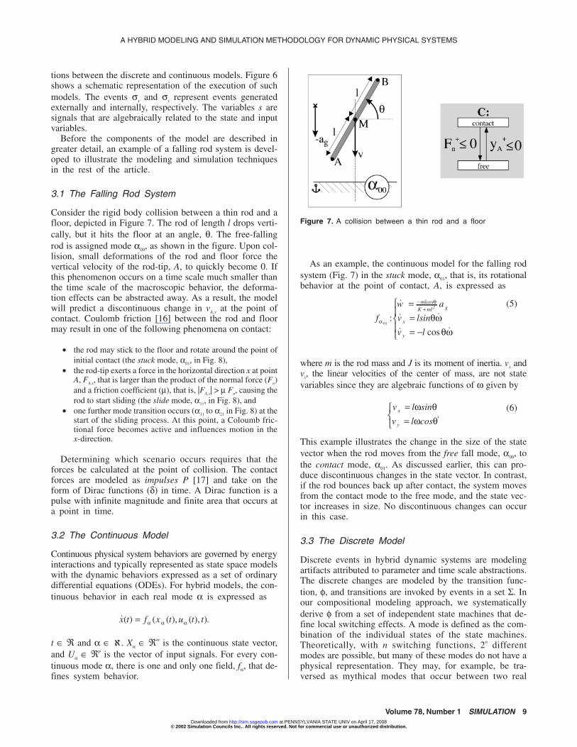
tions between the discrete and continuous models. Figure 6shows a schematic representation of the execution of suchmodels. The events σx and σs represent events generatedexternally and internally, respectively. The variables s aresignals that are algebraically related to the state and inputvariables.

Before the components of the model are described ingreater detail, an example of a falling rod system is devel-oped to illustrate the modeling and simulation techniquesin the rest of the article.

3.1 The Falling Rod System

Consider the rigid body collision between a thin rod and afloor, depicted in Figure 7. The rod of length l drops verti-cally, but it hits the floor at an angle, θ. The free-fallingrod is assigned mode α00, as shown in the figure. Upon col-lision, small deformations of the rod and floor force thevertical velocity of the rod-tip, A, to quickly become 0. Ifthis phenomenon occurs on a time scale much smaller thanthe time scale of the macroscopic behavior, the deforma-tion effects can be abstracted away. As a result, the modelwill predict a discontinuous change in vA,y at the point ofcontact. Coulomb friction [16] between the rod and floormay result in one of the following phenomena on contact:

• the rod may stick to the floor and rotate around the point ofinitial contact (the stuck mode, α01, in Fig. 8),

• the rod-tip exerts a force in the horizontal direction x at pointA, FA,x, that is larger than the product of the normal force (Fn)and a friction coefficient (µ), that is, |FA,x| > µ Fn, causing therod to start sliding (the slide mode, α11, in Fig. 8), and

• one further mode transition occurs (α11 to α21 in Fig. 8) at thestart of the sliding process. At this point, a Coloumb fric-tional force becomes active and influences motion in thex-direction.

Determining which scenario occurs requires that theforces be calculated at the point of collision. The contactforces are modeled as impulses P [17] and take on theform of Dirac functions (δ) in time. A Dirac function is apulse with infinite magnitude and finite area that occurs ata point in time.

3.2 The Continuous Model

Continuous physical system behaviors are governed by energyinteractions and typically represented as state space modelswith the dynamic behaviors expressed as a set of ordinarydifferential equations (ODEs). For hybrid models, the con-tinuous behavior in each real mode α is expressed as

�( ) ( ( ), ( ), )x t f x t u t t= α α α .

t ∈ ℜ and α ∈ ℵ. Xα ∈ ℜm is the continuous state vector,and Uα ∈ ℜp is the vector of input signals. For every con-tinuous mode α, there is one and only one field, fα, that de-fines system behavior.

As an example, the continuous model for the falling rodsystem (Fig. 7) in the stuck mode, α01, that is, its rotationalbehavior at the point of contact, A, is expressed as

f

w a

v l

v l

mlg

x

y

α

θ

θωθω

01:

�

� �

� cos �

=== −

− cos

K +ml 2

sin

(5)

where m is the rod mass and J is its moment of inertia. vx andvy, the linear velocities of the center of mass, are not statevariables since they are algebraic functions of ω given by

v l

lx ==

ω θω θ

sin

v cosy

.(6)

This example illustrates the change in the size of the statevector when the rod moves from the free fall mode, α00, tothe contact mode, α01. As discussed earlier, this can pro-duce discontinuous changes in the state vector. In contrast,if the rod bounces back up after contact, the system movesfrom the contact mode to the free mode, and the state vec-tor increases in size. No discontinuous changes can occurin this case.

3.3 The Discrete Model

Discrete events in hybrid dynamic systems are modelingartifacts attributed to parameter and time scale abstractions.The discrete changes are modeled by the transition func-tion, φ, and transitions are invoked by events in a set Σ. Inour compositional modeling approach, we systematicallyderive φ from a set of independent state machines that de-fine local switching effects. A mode is defined as the com-bination of the individual states of the state machines.Theoretically, with n switching functions, 2n differentmodes are possible, but many of these modes do not have aphysical representation. They may, for example, be tra-versed as mythical modes that occur between two real

Volume 78, Number 1 SIMULATION 9

A HYBRID MODELING AND SIMULATION METHODOLOGY FOR DYNAMIC PHYSICAL SYSTEMS

Figure 7. A collision between a thin rod and a floor

© 2002 Simulation Councils Inc.. All rights reserved. Not for commercial use or unauthorized distribution. at PENNSYLVANIA STATE UNIV on April 17, 2008 http://sim.sagepub.comDownloaded from

modes of operation. An important contribution of our workis to establish execution semantics that handle these se-quences of mode changes correctly.

The discrete model can be implemented by Petri nets orfinite state machines. It is represented as

• I = {α0, . . ., αk} is a set of states describing the modes of thesystem.

• Σ = {σ0, . . ., σl} is the set of events that can cause state transi-tions. Events are generated from signal values in the physicalprocess (Σs), or they can be external control signals (Σx),Σ=Σs

× Σx.• φ: I × Σ→ I represents a discrete state transition function that

defines the new mode after an event occurs.

3.4 Interactions

Interactions between the continuous and discrete modelsare specified by (1) events generated in the continuousmodel and (2) mode changes defined by the discretemodel. More formally they can be expressed as

• S ∈ ℜn, the signals used for event generation.• h : X ×U × I→ S, returns signals from the input and state vari-

able values in a given mode.• g : X × I→X+, computes the a posteriori state vector, X+, in the

new mode from the a priori state vector, X. There may be a dis-continuous change from X to X+.

• γ : S × S+ → Σs, generates discrete events, Σs, from the signalvalues. These signal values may be computed from the a pri-ori state vector, S, or the a posteriori state vector, S+.

The function γ generates discrete events when signals crossprespecified threshold values. The collision transition forthe falling rod is defined by the following constraints:

γσσ

: ,y v

FA A y contact

n free

+

+

≤ ∧ < ⇒≤ ⇒

0 0

0.

(7)

The output function, h, computes the values of these sig-nals from the continuous state vector. For the signals usedin the collision transition for the falling rod, this yields

h

y v dt l

v m v l

Fm v a

A y

A y y

ny g

: (

(� )

,

= −= +

=−

∫ sin

cos

θω θ

α0 00if

otherwise

.

(8)

The generated events applied to the model may indicatethat the system changes its mode of continuous operation.When mode switching occurs, the continuous state vectorof the system may change. The function g transforms thecontinuous state vector as mode changes occur. In general,these transformations may be hard to derive, but for physi-cal system models, this function has to satisfy the principleof conservation of state. When the falling rod first makescontact with the floor, conservation of state is applied toderive the state vector transformation function [5]:

10 SIMULATION Volume 78, Number 1

P. J. Mosterman and G. Biswas

Figure 8. Two possible scenarios after collision

© 2002 Simulation Councils Inc.. All rights reserved. Not for commercial use or unauthorized distribution. at PENNSYLVANIA STATE UNIV on April 17, 2008 http://sim.sagepub.comDownloaded from

g v l

v l

J ml v v

J ml

x

y

y x

α

ω θ θωω θ01

2

:

( )+ − −

++ +

+

=== −

cos sin

sin

ω θ+

cos

.

(9)

In mode α00, the rod has three degrees of freedom, and thestate mapping does not cause discontinuous changes:

g v v

v vx x

y y

α

ω ω00 :

+

+

+

===

.

(10)

4. Abstractions in Physical System Models

Previous work [2, 3] formulated a systematic approach tohybrid modeling of dynamic physical systems using a hy-brid bond graph formulation. Bond graphs are a languagefor building topological models of physical systems basedon energy exchange between components of the system[8]. System components model physical phenomena, suchas energy storage (capacitive and inertial elements), dissi-pation (resistive elements), and energy transformation be-tween domains (transformer and gyrator elements). Hybridbond graphs introduce switching mechanisms that causedynamic changes in the topological model structure duringbehavior evolution.

Schemes were developed to express switching specifica-tions between the configurations (modes) as conditionsbased on state variables. Switching conditions may beexpressed in terms of the state variables immediatelybefore switching occurred (a priori values), or in terms ofstate variables computed by solving the initial value prob-lem for the newly activated mode (a posteriori values). Thea priori and a posteriori values may differ when the dimen-sions of the state vector change from one mode to another.

4.1 Abstractions

Previous work [3, 4, 18] identified two types of abstractionphenomena that lead to discontinuities in physical systemmodels: (1) parameter abstraction and (2) time scale ab-straction. In this article, it is shown that switching condi-tions that result from parameter abstractions have to be interms of a posteriori values, and conditions due to timescale abstraction have to be in terms of a priori values.

4.1.1 Parameter Abstraction

Parameter abstractions occur when small dissipation andstorage elements are ignored to simplify the system model.This may cause discontinuous changes in system behavior.

Consider the example of the rigid body collisionbetween the rod and the floor from Figure 7. The systemneeds to be analyzed to determine the mode on contact.This requires calculation of the forces at the point of colli-sion. As discussed, the contact forces are impulses, P, thattake on the form of Dirac pulses (δ) in time. The area of

the impulse functions at the point of impact is determinedby the state vectors immediately prior to the impact, x, andimmediately after the impact, x+.

To calculate x+, the principle of conservation of state isapplied, which requires that the exchange of momentumbetween the linear and angular inertias upon impact doesnot generate or annihilate momentum [4, 5]. Upon contact,mode α01, the linear velocities of the center of mass, vx andvy, are completely determined by the angular velocity, ω:

v l

lx+ +

+

== −

ω θω θ

sin

v cosy+

.(11)

Conservation of momentum yields the new state vector [2,4]

ωω θ θ+ =

− −

+

J ml v v

J ml

y x( )cos sin2

,(12)

where J is the rod inertia, m is its mass, and l is its length.These a posteriori values may be such that the impulsescorresponding to the forces FA,x and Fn result in |PA,x| > µ Pn

and the rod starts to slide (mode α11). In this mode, the hor-izontal velocity v x

+ is not algebraically dependent on ω, but

the vertical velocity is; that is, v y+ = –lω+ cosθ holds. Thus,

the rod tip moves freely in the x-direction. Its vertical mo-mentum immediately before contact (mode α00) is distrib-uted over its a posteriori (after impact) angular velocityand a posteriori vertical momentum to ensure yA does notchange (i.e., the constraint to keep it in contact with thefloor holds). In Figure 8, the transition conditions betweenmodes α11 (slide) and α01 (stuck) are defined by automataS, where vth represents a small threshold value.

If the continuous state vector in the sliding mode, α11,was computed from the previously inferred mode, α01, thedependence of v x

+ on ω+ in that mode would result in a hor-izontal velocity associated with its center of mass, whichwould keep the rod tip from moving in the x-direction aswell. That would be physically incorrect. So the consecu-tive mode switch to α11 has to occur before the state vectoris updated to its a posteriori values, x = x+. Mathematically,this can be represented as

x g x

x x

x f x t

x x

+

+

===

→+

α

α

α

γαα

1

1

1

12( )

� ( , )

( , )

� ��� ���

x g x

x g x

x x

x

x x

+

+

+

=

→=

=+

α

α

γα

αα

2

2

23

3

( )

( )

�

( , )

� ��� ���

=

f x tα

α

3

3

( , )

,

� ��� ���

(13)

Volume 78, Number 1 SIMULATION 11

A HYBRID MODELING AND SIMULATION METHODOLOGY FOR DYNAMIC PHYSICAL SYSTEMS

© 2002 Simulation Councils Inc.. All rights reserved. Not for commercial use or unauthorized distribution. at PENNSYLVANIA STATE UNIV on April 17, 2008 http://sim.sagepub.comDownloaded from

where α2 is a so-called mythical mode [5, 13].It is clear that switching in this example has to be based

on x+ rather than x (see Figs. 7 and 8). Figure 7 shows theconstraint that achieves the contact mode of operation. Aslong as the rod exerts a downward force on the floor, itstays in contact. If the normal force, Fn, becomes negative,the rod disconnects and lifts off the floor. In the slidingmode, α11, vA,x ≠ 0; therefore, there is a Coloumb frictionforce Ff in the opposite direction. This force changes dis-continuously at vA,x = 0 and that causes another immediatemode change to α21. This is illustrated in Figure 9, whichshows the three modes of the Coulomb friction characteris-tic. In mode 1, the horizontal velocity is 0 and the force atthe contact point is free but limited by a breakaway forcethat in general is larger than the constant friction force, Ff,in one of the sliding modes. In mode 2, there is a negativehorizontal velocity and a constant friction force acting.Mode 3 is similar.

4.1.2 Time Scale Abstraction

Time scale abstractions are applied to behaviors that occuron a small time scale. The behavior is not abstracted awaybut compressed to occur at a point in time, and this mayagain cause discontinuous changes in the system behavior.

Consider the perfectly elastic collision of two bodies.Mass m1 moving with linear velocity v1 collides with massm2 moving with velocity v2 (see Fig. 10). In general, thecollision phenomenon is governed by the principle of con-servation of momentum. Using m1 = m2 yields

v 2+ + v1

+ = v2 + v1, (14)

where v1 and v2 are the velocities of the masses before col-lision, and v1

+ and v 2+ are their velocities after collision.

In detail, the collision process includes elasticity effectsthat store and return the kinetic energy of the masses overa short period of time. Because the time scale of this phe-nomenon is very small compared with the behavior of in-terest, it can be modeled as an instantaneous change at apoint in time governed by the restitution equation:

v 2+ – v1

+ = –ε (v2 – v1), (15)

where ε, the coefficient of restitution, is typically a func-tion of v1 and v2. Combining eqs. (14) and (15) results in

v v v

v v v1

12 1

12 2

21

2 11

2 2

+ −∈ + ∈

+ + ∈ −∈

= += +

.(16)

This algebraic relation only holds at a point in time. There-fore, the switching specifications have to ensure that thecollide mode is departed immediately after the state vectoris updated, x = x+. Mathematically, this is represented as

x g x

x x

x f x t

x x

+

+

===

→+

α

α

α

γαα

1

1

1

12( )

� ( , )

( , )

� ��� ���

x g x

x x

x g x

xx x

+

+

+

==

→=

=+

α

α

γα

αα

2

2

23

3

( )

( )( , )

� ��� ���

x

x f x t

+

=

� ( , )α

α

3

3

� ��� ���

,

(17)

where α2 is a pinnacle. Figure 10 illustrates that switchingspecifications have to be in terms of a priori state variablevalues. Moreover, a switching specification such as is usedfor the falling rod to make the bodies disconnect when theforce between them becomes negative, F12 < 0, cannot beapplied here because on collision F12 > 0, and the con-straint would not move the system of bodies into a freemode immediately after collision. Thus, �x = fα(x,t) wouldbe executed, but fα does not exist for the collision modewhere behavior is defined by algebraic relations, see eq.(16).

4.1.3 Summary

The two types of abstraction have a distinctly different ef-fect on how to formulate switching specifications and in-troduce the fundamentally different behavior betweenmythical modes and pinnacles. Parameter and time scaleabstractions have been applied to a number of examples.The diode inductor example presented in the Introduction,and analyzed in greater detail in other work [6], is anotherapplication of parameter abstraction. Parameter abstrac-tions have also been applied to clutch and braking systems

12 SIMULATION Volume 78, Number 1

P. J. Mosterman and G. Biswas

Figure 9. Coulomb friction causes physical events

Figure 10. A collision between two bodies

© 2002 Simulation Councils Inc.. All rights reserved. Not for commercial use or unauthorized distribution. at PENNSYLVANIA STATE UNIV on April 17, 2008 http://sim.sagepub.comDownloaded from

[7]. A realistic application of time scale abstractions hasbeen in modeling of hydraulic actuators of aircraft attitudecontrol systems [19].

Time scale abstraction collapses behavior during smallintervals into points, and the switching model uses a prioristate values. In contrast, parameter abstraction abstractsaway complex nonlinear behaviors, which are modeled byswitching conditions based on a posteriori state valuescomputed by gα

β . The mythical modes that result fromthese conditions are modeling artifacts and have no realrepresentation, and, therefore, do not affect the state vector,x. This is called the principle of invariance of state [2].

Mythical modes can be replaced by direct transitions tothe final real mode (either a pinnacle, Pα, or a continuousmode, Fα). However, finding these direct transitionsrequires considerable effort and because of its global char-acter needs to be performed whenever local changes to themodel are made. A more pragmatic approach is to incorpo-rate systematic techniques in the compositional modelingformalism to deal with these artifacts. Furthermore, trans-lating a system model into a model where only a prioristate variable values are used complicates the model verifi-cation task considerably. If a posteriori values are used,invariance of state can be conveniently applied for modelverification purposes [3].

4.2 Physical Model Semantics

A mathematical model can now be presented that embod-ies the physical abstraction semantics. It relies on a switch-ing function γ α

β that depends on values xα prior to thejump, and values xα

+ just after the jump. The semantics arespecified by the recursive relation between γ α

β and gαβ ,

which takes the form

x g x

x xk k

i

k

i

i

k k

α αα

α

αα

α αγ

+

+

=≤

+

( )

( , )1 0.

(18)

Note the αk subscript of xkα in g x

k

i

kαα

α( ). In physical sys-

tems, continuous behavior is completely specified by thestate. Therefore, the state mapping is independent of thedeparted mode, that is, gα

β is independent of α. This resultsin the general sequence

x g x

x x

x f x t

x x

+

+

===

→+

α

α

α

γαα

1

1

1

12( )

� ( , )

( , )

� ��� ���

x g x

x x

x f x t

x x

+

+

===

→+

α

α

α

γαα

2

2

2

23

( )

� ( , )

( , )

� ��� ���

�

� ���

→=

==

−+

+

+γ

α

α

α

αα

mm

m

m

m

x xx g x

x x

x f x t

1( , )

( )

� ( , )���

.

(19)

In this sequence, each mode, α, may be departed when anyof the three assignment statements is executed. The differ-

ence between eq. (3) and eq. (19) is the use of (x,x+) as ar-gument to γ α

β . A block diagram of the resultant operationof a hybrid system corresponding to the 9-tuple model dis-cussed in Section 3 is presented in Figure 11. The modelincludes the semantic specifications developed in the lastsection. In relation to the model in Figure 6, there is an ad-ditional feedback, x+, from g to γ.

Overall, three execution cases can be distinguished (Fig.12):

1. Mythical mode: This occurs when x+ = g iα (x) leadsto γ α

αi

i x x+ + ≤1 0( , ) . The immediate transition causedby x+ bypasses the integrator (∫) element and thestate vector, x, remains unchanged through the transi-tion. As shown in Figure 12(a), mythical modes canoccur in the loops(i) φ → h → γ. This corresponds to mythical modes

with no discontinuous changes in the state vector.(ii) φ → g → h → γ. This corresponds to mythical

modes with discontinuous changes in the statevector.

2. Pinnacle: This occurs when x = x+ results inγ αα

i

i x x+ + ≤1 0( , ) . Updating of x stored by the ∫ ele-

ment causes a mode transition, and, therefore, mode

Volume 78, Number 1 SIMULATION 13

A HYBRID MODELING AND SIMULATION METHODOLOGY FOR DYNAMIC PHYSICAL SYSTEMS

Figure 11. A general hybrid system

© 2002 Simulation Councils Inc.. All rights reserved. Not for commercial use or unauthorized distribution. at PENNSYLVANIA STATE UNIV on April 17, 2008 http://sim.sagepub.comDownloaded from

αi only exists at a point in time. In Figure 12(b), pin-nacles are shown to arise from the φ → g → ∫ → h→ γ loop since they require the state vector to beupdated in the ∫ element.

3. Continuous mode: This occurs when � ( , )x f x t=results in γ α

αi

i x x+ + >1 0( , ) . The system goes into aperiod of continuous evolution, until γ α

αi

i x x+

+ ≤1

0( , ) ,and the mode is departed. In Figure 12(c), continuousmodes arise from the φ → f → ∫ → h → γ loop whileg is not part of this loop because x+ = x during con-tinuous behavior.

Pinnacles and continuous modes are also referred to asreal modes because they change x stored by the ∫ element.Comparison with the general sequence in eq. (3) showsthat the gα

β operation can be associated with the transitionor the new mode. In this article, gα

β is associated withmodes for two reasons: (1) it affects the energy distributionin the system, and therefore it should correspond to a phys-ical mode of operation, and (2) for mythical mode transi-tions, the state vector x remains unchanged; therefore, itmakes it easier to implement a simulator if g is associatedwith a mode rather than a transition.

5. The Hybrid Dynamic System Simulator

The hybrid dynamic simulator implements the model ofFigure 11. The integrator is the core of the continuous sim-ulation component. To simplify the implementation, a for-ward Euler integrator that approximates derivatives by�x x x

tk k= + −1

∆ or xk+1 = f∆t + xk is used, though in principle any

solver with a root-finding mechanism can be used. Forexample, the state equations in eq. (5) would be imple-mented as

f

a t

v l

v

k J ml g k

x k k k

y

k

α

θω ωθ ω

01

21

1 1 1: ,

,

+−+

+ + +

= +=

cos

sin

∆

k k kl+ + += −

1 1 1cosθ ω

(20)

(ag represents the gravitational constant, the accelerationdue to gravity).

The h function is implemented in a similar manner

h

y y l

v v lA M k

A x x k k

:

,

, ,

++

+

++

++

= −= −

1

1 1

sin

sink +1+

k +1+

θθ ω

( )

+

+−

= +

= −++

v v l

Fm a

A y y k k k

n v v

t gy k y k

, ,

, ,

cosθ ωα0 00

1

if

oth∆ erwise

if

otherwise

=

+−+

+FmA x v v

tx k x k, , ,

0 00

1

α

∆

.

(21)

The derivative terms in Fn and FA,x may produce Diracpulses and are termed hd. The remaining terms are part ofhi. If no discontinuous changes occur (e.g., v y k, +

+1 = vy,k+1),

the forces Fn and FA,x can be estimated numerically usingthe above equation. When discontinuous changes occur(e.g., v y k, +

+1 ≠ vy,k+1), the derivative term is a Dirac pulse of

infinite magnitude that dominates all the other terms in theequation. However, the numerical approximation may com-pute a pulse magnitude that does not dominate the otherterms in the equation, and this would result in incorrectsimulation results. Therefore, discontinuous changes aretracked separately, and when they occur, their time deriva-tive terms are replaced by Dirac pulses. Algorithm 1 im-plements the derSignal function. If ∆T = 0 for a pinnacle,

14 SIMULATION Volume 78, Number 1

P. J. Mosterman and G. Biswas

Figure 12. Classes of modes of operation

© 2002 Simulation Councils Inc.. All rights reserved. Not for commercial use or unauthorized distribution. at PENNSYLVANIA STATE UNIV on April 17, 2008 http://sim.sagepub.comDownloaded from

or if hd(x+, α) ≠ hd(x, α) for a discontinuous change, the

area of the corresponding Dirac pulse is returned. Other-wise, no discontinuous changes have occurred, and the Eu-ler approximation is returned as the value of the derivative.

Algorithm 2 is the primary simulation module. Therecursive relation, eq. (18), is implemented as functionselMode (Algorithm 3), executed twice for each time step:(1) when continuous evolution terminates in a new mode,4

and (2) when pinnacles are traversed, and the ∆T argumentin Algorithm 3 is set to 0.

Algorithm 1 derSignal ( , , , , )x x x Tk k k m++

+1 1 α ∆if ∆T = 0 then

s = hi(xk+1, αm)else

s = (hd(xk+1, αm) – hd(xk, αm))/∆T + hi(xk+1, αm)end ifif ∆T h x h xd k m d k m= ∨ ≠+

++0 1 1( , ) ( , )α α then

s h x h xd k m d k m+

++

+= −( , ) ( , )1 1α αelse

s h x h x T h xd k m d k m i k m+

++

++= − +( ( , ) ( , )) / ( , )1 1α α α∆

end if

Algorithm 2 Hybrid Simulationx x x x x xk k k k k+ +

++ += = =1 1 1 10( ); ;

t t= ←0;δ Simulation time stepα αm k k kselMode x x x+ +

++=1 1 1 0 0( , , , , )

if α αm + ≠1 0 thenrepeat

x xk k+ ++=1 1

α αm m= +1

α αm k k k mselMode x x x+ ++

+=1 1 1 0( , , , , )until α αm m+ =1

end if {Initialization Completed}repeat

t t t= +δx f x t tk k+ =1 ( , )δx xk k++

+=1 1

α αm k k k mselMode x x x+ ++

+=1 1 1 0( , , , , )

if α αm + ≠1 0 thenrepeat

x xk k+ ++=1 1

α αm m= +1

α αm k k kselMode x x x+ ++

+=1 1 1 0 0( , , , , )until α αm m+ =1

end ifx xk k= +1

until simulation end

Algorithm 3 selMode x x x Tk k k m( , , , , )++

+1 1 α ∆a derSignal x x x Tm m k k k m+ +

++=1 1 1φ α α( , ( , , , , ))∆

if α αm m+ ≠1 thenx g xk k

m

++

+= +1 1

1α ( )ret val selMode x x x Tk k k m_ ( , , , , )= +

++ +1 1 1α ∆

elseret val m_ = α

end if

The simulated trajectories of the rod in phase space forthree different values of the friction coefficient (µ) areshown in Figure 13. The system is initialized with zeroangular and linear velocities (vx, vy, ω) = (0,0,0). Becauseof the orientation of the coordinate system of the rod, theposition of the rod tip, point A, is at a negative value of l.Once the rod is released, flow Fα 00

applies, and the magni-tude of its vertical velocity increases in time. When the rodtip, A, touches the floor, the rod may start to slide, gov-erned by flow Fα 21

(happens for µ = 0.26 and µ = 0.265),or it may get stuck and behavior is governed by flow Fα 01

(happens for µ = 0.27). The discontinuous jumps betweenflows are illustrated in Figure 13. Also, for simulationswith µ = 0.26 and µ = 0.265, the sliding mode, α21 is acti-vated immediately after α00 because a force balance com-putation indicates that the stuck mode α01 is departedinstantaneously; that is, it has no real existence at the pointof collision.

Volume 78, Number 1 SIMULATION 15

A HYBRID MODELING AND SIMULATION METHODOLOGY FOR DYNAMIC PHYSICAL SYSTEMS

Figure 13. A number of trajectories in phase space of the colliding rod, vth = 0.2, θ = 0.85, l = –1.0, y0 = 1.5

4. Precision is improved by varying δt and employing a bisectionalsearch.

© 2002 Simulation Councils Inc.. All rights reserved. Not for commercial use or unauthorized distribution. at PENNSYLVANIA STATE UNIV on April 17, 2008 http://sim.sagepub.comDownloaded from

16 SIMULATION Volume 78, Number 1

When sliding, the center of mass of the rod acceleratesin the horizontal direction, and the magnitude of the negativevelocity at the rod tip decreases. When it falls below athreshold value, transition conditions determine that the rodgets stuck, which implies a mode change to α01 and flowFα 01

. The transition conditions had to be properly specifiedso that the system does not go into a loop of instanta-neous mode changes (sliding and stuck), which would vio-late the physical principle that system behavior mustevolve in time [2, 3].

6. Conclusions

This article presents a formal mathematical framework foranalyzing hybrid behaviors and uses the framework to de-velop a methodology for simulating behaviors of dynamicphysical systems. This extends previous work oncompositional modeling of hybrid systems combining bondgraph models with local discrete finite state automata [3,7]. Parameter and time scale abstractions are the key to de-veloping systematic switching specifications that are gov-erned by both a priori and a posteriori state vector values.Hybrid dynamic behaviors are piecewise continuous andcombine continuous behavior over intervals of time withpinnacles that represent a real behavior at a point in time(time scale abstraction) and mythical modes that have noreal existence on the timeline (artifact of parameter ab-straction). The formal model specifications are made up ofthree components, (1) the continuous model, (2) the dis-crete model, and (3) the interaction model, and define amethodology for developing hybrid dynamic models ofphysical systems. A hybrid dynamic simulator is developedas a combination of three algorithms from the mathemati-cal execution semantics.

State vectors variable values have to satisfy the principleof invariance of state across mythical mode changes,whereas discontinuous changes in state variables that occurat pinnacles are derived using the principle of conservationof state and explicitly defined interactions with the envi-ronment (represented as Dirac pulses). When modechanges occur, global specifications are derived dynami-cally from local switching functions. The use of local spec-ifications often results in the system going through asequence of discrete changes, but the modeling task is sim-plified because compositional modeling principles can beapplied. This contrasts other approaches that have beenemployed for hybrid modeling (e.g., [12]), which requirepredefined global specifications of continuous systembehavior in terms of differential equations. Currentresearch efforts are directed toward extending this method-ology to design and analysis of embedded (computer-based) control of complex physical systems [6, 8].

The hybrid bond graph modeling and simulation algo-rithms have been integrated into a software package calledHYBRSIM [20]. This package, implemented in Java, can beaccessed on the Web from http://www.op.dlr.de/~pjm/hybrsim. HYBRSIM establishes a formal framework andserves as a precursor to an object-oriented implementationas part of the Modelica modeling language [21].

7. Acknowledgments

The authors would like to thank the two anonymous review-ers for their valuable suggestions in improving this article.

8. References

[1] Paynter, Henry M. 1961. Analysis and design of engineering systems.Cambridge, MA: MIT Press.

[2] Mosterman, Pieter J. 1997. Hybrid dynamic systems: A hybrid bondgraph modeling paradigm and its application in diagnosis. PhDdissertation, Vanderbilt University, Nashville, TN.

[3] Mosterman, Pieter J., and Gautam Biswas. 1998. A theory of disconti-nuities in dynamic physical systems. Journal of the Franklin Insti-tute 335B (3): 401-39.

[4] Mosterman, Pieter J., and Gautam Biswas. 2000. A comprehensivemethodology for building hybrid models of physical systems. Arti-ficial Intelligence 121:171-209.

[5] Mosterman, Pieter J., and Gautam Biswas. 1997. Formal specifica-tions for hybrid dynamical systems. Paper presented at IJCAI-97,pp. 568-73, August, Nagoya, Japan.

[4] Cellier, F. E., H. Elmqvist, and M. Otter. 1991. Modelling from physi-cal principles. In The control handbook, edited by W. S. Levine,pp. 99-107. Boca Raton, FL: CRC Press.

[5] de Vries, Theo J. A., Peter C. Breedveld, and Piet Meindertsma. 1993.Polymorphic modeling of engineering systems. Paper presented atProceedings of the International Conference on Bond GraphModeling, pp. 17-22, San Diego, CA.

[6] Mosterman, Pieter J., Gautam Biswas, and Janos Sztipanovits. 1998.A hybrid modeling and verification paradigm for embedded con-trol systems. Control Engineering Practice 6:511-21.

[7] Mosterman, Pieter J., Gautam Biswas, and Martin Otter. Simulation ofdiscontinuities in physical system models based on conservationprinciples. Paper presented at SCS Summer Simulation Confer-ence, July, Reno, CA.

[8] Mosterman, Pieter J., Feng Zhao, and Gautam Biswas. 1999. Slidingmode model semantics and simulation for hybrid systems. InHybrid systems V, lecture notes in computer science, edited by P.Antsalelis, W. Kohn, M. Lemmon, A. Nerode, and S. Sastry, pp.218-37. New York: Springer-Verlag.

[9] Deshpande, Akash, and Pravi Varaiya. 1995. Viable control of hybridsystems. In Hybrid systems II, edited by Panos Antsaklis, WolfKohn, Anil Nerode, and Shankar Sastry, vol. 999, pp. 128-47. Lec-ture Notes in Computer Science. New York: Springer-Verlag.

[10] Guckenheimer, John, and Stewart Johnson. 1995. Planar hybrid sys-tems. In Hybrid systems II, edited by Panos Antsaklis, Wolf Kohn,Anil Nerode, and Shankar Sastry, vol. 999, pp. 202-25. LectureNotes in Computer Science. New York: Springer-Verlag.

[11] Rudin, W. 1976. Principles of mathematical analysis. 3rd ed. NewYork: McGraw-Hill.

[12] Alur, R., C. Courcoubetis, N. Halbwachs, T. A. Henzinger, P.-H. Ho,X. Nicollin, A. Olivero, J. Sifakis, and S. Yovine. 1994. The algo-rithmic analysis of hybrid systems. In Proceedings of the 11thInternational Conference on Analysis and Optimization of Dis-crete Event Systems, edited by J. W. Bakkers, C. Huizing, W. P. deRoeres, and G. Rozenberg, pp. 331-51. Lecture Notes in Controland Information Sciences 199. New York: Springer-Verlag.

[13] Nishida, T., and S. Doshita. 1987. Reasoning about discontinuouschange. Paper presented at Proceedings AAAI-87, pp. 643-8, Seat-tle, WA.

[14] Alur, Rajeev, Costas Courcoubetis, Thomas A. Henzinger, andPei-Hsin Ho. 1993. Hybrid automata: An algorithmic approach tothe specification and verification of hybrid systems. In Lecturenotes in computer science, edited by R. L. Grossma, A. Nerode,A. P. Ravn, and H. Rischel, vol. 736, pp. 209-29. New York:Springer-Verlag.

[15] Lennartson, Bengt, Michael Tittus, Bo Egardt, and Stefan Pettersson.1996. Hybrid systems in process control. IEEE Control Systems,October, pp. 45-56.

P. J. Mosterman and G. Biswas

© 2002 Simulation Councils Inc.. All rights reserved. Not for commercial use or unauthorized distribution. at PENNSYLVANIA STATE UNIV on April 17, 2008 http://sim.sagepub.comDownloaded from

[16] Lötstedt, P. 1981. Coulomb friction in two-dimensional rigid bodysystems. Zeitschrift für angewandte Mathematik and Mechanik61:605-15.

[17] Brach, Raymond M. 1991. Mechanical impact dynamics. New York:John Wiley.

[18] Mosterman, Pieter J., and Gautam Biswas. 1997. Principles for mod-eling, verification, and simulation of hybrid dynamic systems.Paper presented at Fifth International Conference on Hybrid Sys-tems, pp. 21-27, September, Notre Dame, IN.

[19] Mosterman, Pieter J., and Gautam Biswas. 1999. Hybrid automatafor modeling discrete transitions in complex dynamic systems.Hybrid Systems: Computation and Control, Lecture Notes in Com-puter Science, vol. 1569, pp. 178-92. The Netherlands: SpringerVerlag.

[20] Mosterman, Pieter J., and Gautam Biswas. 1999. A Java implementa-tion of an environment for hybrid modeling and simulation of dynamicphysical systems physical systems. Paper presented at Proceedingsof ICBGM ’99, pp. 157-62, January, San Francisco, CA.

[21] Mosterman, Pieter J. 2001. MASIM—A Hybrid Dynamic SystemsSimulator. Technical report DLR-IB-515-01-07, Institute ofRobotics and Mechatronics, DLR Oberpfaffenhofen.

Pieter J. Mosterman recently assumed a position as senior researchscientist at The MathWorks, Inc., in Natick, MA. Before, he held a re-search position at the German Aerospace Center (DLR) inOberpfaffenhofen. He has a Ph.D. degree in electrical and computerengineering from Vanderbilt University in Nashville, TN, and aM.Sc. degree in electrical engineering from the University of Twente,Netherlands. His primary research interests are in computer-auto-mated multi-paradigm modeling with principal applications intraining systems and fault detection, isolation, and reconfiguration.For this, he designed several simulation environments, a.o., the Elec-tronics Laboratory Simulator (nominated for The ComputerworldSmithsonian Award), a first version of TRANSCEND, HyBrSim, andMASIM. Specific areas of interest are modeling of physical systems,meta-modeling, and model and formalism transformation to achievea form of higher intelligence in computer-aided control system de-sign (CACSD). An important aspect concerns the behavior genera-tion for heterogeneous models, which requires a hybrid dynamicsystems approach. Dr. Mosterman has served on the program com-mittee of several conferences and workshops and organized special

sessions at the 2001 IEEE Conference on Control Applications, the2000 IEEE International Symposium on CACSD, and Eurosim ’98.He is currently a member of the IFAC Technical Committee onCACSD, chair of the IEEE CSS Action Group on Hybrid DynamicSystems for CACSD, expert reviewer for the European Commission,editor of SIMULATION: Transactions of The Society for Modelingand Simulation International for the area of mechatronics, and asso-ciate editor of the International Journal of Applied Intelligence. Heis also guest editor of special issues of ACM TRANSACTIONS ONMODELING AND COMPUTER SIMULATION and IEEETRANSACTIONS ON CONTROL SYSTEM TECHNOLOGY onthe topic of computer automated multi-paradigm modeling.

Gautam Biswas is an associate professor of Computer Science andEngineering, and Management of Technology at Vanderbilt Univer-sity. He has a Ph.D. in computer science from Michigan State Uni-versity in East Lansing, MI. He conducts research in intelligentsystems with primary interests in hybrid modeling and analysis ofcomplex embedded systems and their applications to diagnosis andfault-adaptive control. He is also involved in developing simula-tion-based environments for learning and instruction. Other re-search areas include Hidden Markov Model techniques forclustering of temporal data sequences and decision-theoretic plan-ning and scheduling for intelligent manufacturing systems. His re-search is currently supported by funding from DARPA, NASA, NSF,and ONR. Dr. Biswas has served on the program committee of anumber of conferences. He was chair of the 1997 IJCAI Workshop onEngineering Problems for Qualitative Reasoning, co-chair of the1996 Principles of Diagnosis Workshop, the 1999 AAAI Spring Sym-posium on Hybrid Systems, and AI, the 2001 Workshop on Qualita-tive Reasoning, Senior Program Committee for AAAI-97 andAAAI-98, and Technical Committee co-chair for the 2000 IEEESMC conference. He is currently an associate editor for the IEEETransactions on Systems, Man, and Cybernetics, IEEE Transactionson Knowledge and Data Engineering, and the International Journalof Applied Intelligence. He is a senior member of the IEEE Com-puter Society, ACM, AAAI, and the Sigma Xi Research Society.

Volume 78, Number 1 SIMULATION 17

A HYBRID MODELING AND SIMULATION METHODOLOGY FOR DYNAMIC PHYSICAL SYSTEMS

© 2002 Simulation Councils Inc.. All rights reserved. Not for commercial use or unauthorized distribution. at PENNSYLVANIA STATE UNIV on April 17, 2008 http://sim.sagepub.comDownloaded from