A hybrid method based on linear programming and variable neighborhood descent for scheduling...

J Glob OptimDOI 10.1007/s10898-014-0185-z

A hybrid method based on linear programmingand variable neighborhood descent for schedulingproduction in open-pit mines

Amina Lamghari · Roussos Dimitrakopoulos ·Jacques A. Ferland

Received: 30 January 2013 / Accepted: 31 March 2014© The Author(s) 2014. This article is published with open access at Springerlink.com

Abstract Production scheduling of open-pit mines is an important problem arising in surfacemine planning as it determines the raw materials to be produced yearly over the life ofthe mine, assesses the value of the mine, and contributes to the sustainable utilization ofmineral resources. Finding the optimal schedule is a complex task, involving large datasets and multiple constraints. This paper introduces a two-phase hybrid solution method.The first phase relies on solving a series of linear programming problems to generate aninitial solution. In the second phase, a variable neighborhood descent procedure is applied toimprove the solution. Upper bounds provided by CPLEX are used to evaluate the efficiencyof the proposed method. Its performance is also assessed by comparing it to recent solutionmethods proposed in the literature and to an alternate method implemented in commercialmine planning software commonly used by professional mine planners. The results of thesecomputational experiments indicate the efficiency of the proposed method and its superiorityover the other methods. It finds excellent solutions (within less than 3.2 % of optimality onaverage) for large instances of the problem in a few seconds up to a few minutes. It alsoprovides new best-known solutions for benchmark instances from the literature, and it cansolve instances recently-published algorithms have found intractable.

Keywords Variable neighborhood descent · Hybrid methods ·Scheduling · Open-pit mine planning

A. Lamghari (B) · R. DimitrakopoulosCOSMO - Stochastic Mine Planning Laboratory, Department of Mining and Materials Engineering,McGill University, FDA Building, 3450 University Street, Montreal, Quebec H3A 2A7, Canadae-mail: [email protected]

R. Dimitrakopoulose-mail: [email protected]

J. A. FerlandDepartment of Computer Science and Operations Research, University of Montreal, C.P. 6128, SUCC.Centre-Ville, Montreal, Quebec H3C 3J7, Canadae-mail: [email protected]

123

J Glob Optim

1 Introduction

Production scheduling of open-pit mines is an important issue in surface mine planning asit determines the raw materials to be produced yearly over the life of the mine, assesses thevalue of the mine, and contributes to the sustainable utilization of mineral resources. Theproblem is complex as it involves large data sets and multiple constraints, placing a strain oncomputational resources.

The mineral deposit is represented as a three-dimensional array of blocks. Each block hasa weight and a metal content estimated using information obtained from drilling. To recoverthe metal, the block must first be extracted from the ground and then treated in a plant. Theseoperations are termed mining and processing, respectively. The set of blocks can be dividedinto two distinct subsets: the set of ore blocks sent to the plant (i.e., blocks that are processedto produce metal), and the set of waste blocks formed by the remaining blocks. Waste blocksare not processed, but the physical nature of the problem requires mining them in order tohave access to ore blocks. Blocks that should be removed to have access to a given block arecalled its predecessors. Each block also has an economic value representing the net profitassociated with it. Hence, for an ore block, this value is equal to the selling revenue less themining and the processing costs. For a waste block, it is equal to minus the cost of miningthe block.

The open-pit mine production scheduling problem (MPSP), also known as the open-pitmine block sequencing problem or the constrained pit limit problem, consists of identifyingwhich blocks should be mined during each period of the life of the mine so as to maximizethe net present value (the total discounted profit) of the mining operation. Decisions on blockscheduling are subject to various constraints, typically:

– Reserve constraints: a block can be mined at most once during the horizon.– Slope constraints: a block cannot be mined before its predecessors.– Mining constraints: the total weight of blocks (waste and ore) mined during each period

of the horizon must not exceed the available extraction equipment capacity, referred to asthe mining capacity.

– Processing constraints: the total weight of ore blocks processed during each period of thehorizon must not exceed the processing plant capacity.

The MPSP can be formulated as a combinatorial optimization problem. Because of itscomplexity and its practical interest, it has been widely studied since the 1960s [21]. For anoverview of the different formulations and solution methodologies, see [23]. As this reviewpaper shows, different solution approaches have been proposed in the literature. These includeexact methods [9,13], heuristics [10,17], and metaheuristics [14,16]. Each approach hasstrengths and weaknesses.

Exact methods solve optimally the MPSP, but their major limitation is that they can onlybe applied to instances of relatively small size. Solving instances of realistic size, where thenumber of blocks is typically in the order of tens to hundreds of thousands, requires prohibitivecomputational times. To reduce the number of binary variables and thus make larger instancescomputationally tractable by exact methods, Ramazan and Dimitrakopoulos [25] propose amixed integer programming formulation where only the variables associated with ore blocksare restricted to be binary. Another approach for handling the large number of binary variablesexploits the structure of the problem to aggregate blocks into groups, leading to a reduction inthe number of variables [5,24]. Aggregation, however, can severely compromise the validityand usefulness of the solution [3]. It causes loss of profitability and may even lead to infeasiblesolutions [5]. In order to reduce the number of binary variables, Bley et al. [4] address a

123

J Glob Optim

different approach involving cutting planes. The authors add to the integer programmingformulation inequalities derived by combining the constraints of the problem to eliminatea number of decision variables from the model prior to optimization. Their results indicatethat adding such inequalities is, in the majority of the cases tested, beneficial for reducing theCPU time required by the solver. However, their experiments were conducted on instancescontaining only hundreds of blocks and 5 or 10 periods.

Heuristics and metaheuristics can tackle large instances of the MPSP in a reasonableamount of time, but they do not guarantee optimality. Their efficiency and robustness canbe improved by combining them with other techniques. A number of such hybrid methodshave been developed over the years. Sevim and Lei [26] and Tolwinski and Underwood [27]combine heuristics with dynamic programming techniques. More recent approaches combineheuristics with exact methods. Moreno et al. [22] introduce an algorithm for solving the linearrelaxation of the MPSP and an LP-based heuristic to obtain feasible solutions. However, thealgorithm proposed by the authors to solve the linear relaxation is only applicable to the variantof the MPSP with a single resource constraint per period and for which such a constraint isan upper bound (i.e., referring to the description given in the beginning of this section, thevariant of the MPSP including either the mining or the processing constraints in addition tothe slope constraints). Bienstock and Zuckerberg [3] propose another algorithm for solvingthe linear relaxation of the MPSP that can handle any number of resource constraints.

Another hybrid approach for the MPSP is the one by Amaya et al. [1]. Starting from aninitial feasible solution generated using Gershon’s heuristic [17], the authors iteratively fixparts of the incumbent solution and re-optimize the ”unfixed” parts. This defines an integerprogramming sub-problem at each iteration that is solved exactly, using the commercialsolver CPLEX. Chicoisne et al. [11] use a similar approach. They first use the method in [22]to generate a feasible solution, followed by an improvement integer programming-basedheuristic, which is an enhanced version of that in [1]. Cullenbine et al. [12] also solve aseries of mixed-integer programs that have fixed variables. The authors consider, however,a variant of the MPSP incorporating lower bounds on mining and processing, which is, asnoted by the authors, harder to solve than the variant where the lower bounds are omitted(i.e., the variant described in the beginning of this section and considered by Chicoisne etal. [11]). The drawback of the recent hybrid algorithms [11,12] is that they rely on timeconsuming integer programming algorithms. The method in [11] can solve instances withup to five million blocks and 15 years but might require 8 h to improve the solution andcannot handle lower bound constraints. On the other hand, the method in [12] can handlelower bound constraints but has been able to tackle only instances with up to 25,000 blocksand 15 periods.

In this paper, we propose a variable neighborhood descent based method for the MPSP.Variable neighborhood descent (VND) is a variant of variable neighborhood search [18]. Thebasic idea is the same: neighborhood change to escape from local optima, but the differentneighborhoods are explored using a best improvement local descent. VND has been showneffective in solving a variety of combinatorial optimization problems (see [8] for an exam-ple). To generate the initial solution to be improved by the VND procedure, we develop adecomposition based heuristic. The basic idea is to reduce the complexity of the problemby exploiting its structure and decomposing it into easier to solve sub-problems. Each sub-problem is associated with one period, and solving it consists of solving a linear program,not an integer or a mixed-integer program. This is followed by a repair heuristic to makethe solution of the sub-problem feasible if necessary. When all sub-problems are considered,their solutions are combined to obtain a feasible solution of the original problem (the initialsolution).

123

J Glob Optim

We applied the method described above to solve two different variants of the MPSP: thevariant described in the beginning of this section, commonly studied in the literature, andthe variant incorporating lower bounds on mining and processing, considered in [12] andknown to be more difficult to solve. For both variants, the computational results indicatethat the proposed solution method is very effective and robust, providing, for all the testedinstances, near-optimal solutions in a few seconds up to a few minutes. It generally out-performs recently-proposed solution methods for the MPSP and provides new best-knownsolutions for benchmark instances from the literature.

From a broad perspective, the method proposed in this paper is a hybrid method combiningmathematical programming algorithms with heuristic search techniques, able to tackle largeinstances of the MPSP. In this sense, it is similar to recent approaches in the literature.However, it has key characteristics which differentiate it from existing methods. First, itdoesn’t resort to aggregation to tackle large instances of the problem. Second, it doesn’t relyon solving a series of integer or mixed integer sub-problems but rather exploits the problemstructure and uses variable neighborhood descent to quickly find improving solutions. Whengenerating the initial solution, it uses an exact method to solve linear programs. Because ofthat, its running time has a slower growth rate compared to recent solution methods in theliterature. Third, it is not a specialized method tailored to solve one variant of the MPSP, but itcan be easily adapted to account for additional constraints. Last but not least, it doesn’t requireany external software, such as CPLEX, in order to be implemented. Indeed, although CPLEXis used in this study to solve the linear programs when generating the initial solution, anymaximum flow algorithm, such as the pseudo-flow algorithm proposed by Hochbaum [19],can be used.

Note that this paper deals with the deterministic version of the MPSP, which assumes thatall the problem parameters are well known. There exist other versions where one or somecomponents of the problem (e.g., prices, metal content, etc.) are not known with certainty.These stochastic versions of the MPSP have received increasing attention in recent years (seefor instance, [2,6,7]).

The remainder of the paper is organized as follows: In Sect. 2 a mathematical formulationof the problem is provided. In Sect. 3 the heuristic for generating an initial solution is outlined.In Sect. 4 the components of the variable neighborhood descent heuristic used to improvethe solution are described. The results of an extensive computational study are presented inSect. 5. This is followed by conclusions in Sect. 6.

2 Mathematical formulation

As mentioned in the introduction, different mathematical formulations of the MPSP havebeen proposed in the literature. In this paper, the integer linear programming formulationproposed by Caccetta and Hill [9] is used. The following notation is used to specify themathematical model:

– T : the scheduling horizon.– t : period index, t = 1, . . . , T .– N : the number of blocks.– i : block index, i = 1, . . . , N .– Pi : the set of predecessors of block i ; i.e., blocks that have to be removed to have access

to block i .– Si : the set of successors of block i ; i.e., s ∈ Si if i ∈ Ps .

123

J Glob Optim

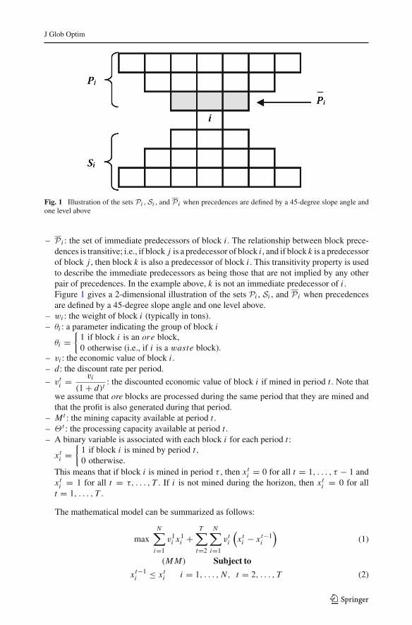
Fig. 1 Illustration of the sets Pi , Si , and P i when precedences are defined by a 45-degree slope angle andone level above

– P i : the set of immediate predecessors of block i . The relationship between block prece-dences is transitive; i.e., if block j is a predecessor of block i , and if block k is a predecessorof block j , then block k is also a predecessor of block i . This transitivity property is usedto describe the immediate predecessors as being those that are not implied by any otherpair of precedences. In the example above, k is not an immediate predecessor of i .Figure 1 gives a 2-dimensional illustration of the sets Pi , Si , and P i when precedencesare defined by a 45-degree slope angle and one level above.

– wi : the weight of block i (typically in tons).– θi : a parameter indicating the group of block i

θi ={

1 if block i is an ore block,0 otherwise (i.e., if i is a waste block).

– vi : the economic value of block i .– d: the discount rate per period.

– vti = vi

(1 + d)t: the discounted economic value of block i if mined in period t . Note that

we assume that ore blocks are processed during the same period that they are mined andthat the profit is also generated during that period.

– Mt : the mining capacity available at period t .– Θ t : the processing capacity available at period t .– A binary variable is associated with each block i for each period t :

xti =

{1 if block i is mined by period t,0 otherwise.

This means that if block i is mined in period τ , then xti = 0 for all t = 1, . . . , τ − 1 and

xti = 1 for all t = τ, . . . , T . If i is not mined during the horizon, then xt

i = 0 for allt = 1, . . . , T .

The mathematical model can be summarized as follows:

maxN∑

i=1

v1i x1

i +T∑

t=2

N∑i=1

vti

(xt

i − xt−1i

)(1)

(M M) Subject to

xt−1i ≤ xt

i i = 1, . . . , N , t = 2, . . . , T (2)

123

J Glob Optim

xti ≤ xt

p i = 1, . . . , N , p ∈ P i , t = 1, . . . , T (3)

N∑i=1

wi x1i ≤ M1 (4)

N∑i=1

wi

(xt

i − xt−1i

)≤ Mt t = 2, . . . , T (5)

N∑i=1

θiwi x1i ≤ Θ1 (6)

N∑i=1

θiwi

(xt

i − xt−1i

)≤ Θ t t = 2, . . . , T (7)

xti = 0 or 1 i = 1, . . . , N , t = 1, . . . , T . (8)

The objective function (1) to be maximized is equal to the net present value of the miningoperation. Constraints (2) guarantee that each block i is mined at most once during thehorizon (reserve constraints). The mining precedence (slope constraints) is enforced byconstraints (3). Constraints (4) and (5) impose an upper bound Mt on the amount of material(waste and ore) mined during each period t (mining constraints). Constraints (6) and (7)ensure that the amount of ore processed during each period does not exceed the processingcapacity available at that period (processing constraints).

The solution procedure, which includes two phases, is described in the next sections.

3 Phase 1 to construct an initial feasible solution (SH)

In this section, a general overview of the algorithm used to generate an initial feasible solutionis first presented. This is followed by a step-by-step description of it.

3.1 Overview of the algorithm

The sub-problems associated with the periods t (t = 1, . . . , T ) are solved sequentially (inincreasing order of t), and the solutions of the sub-problems are combined to generate theinitial solution. The procedure to deal with the sub-problem associated with each period tcan be summarized as follows: First, a set of blocks to be mined in t is identified by solvinga linear programming model. This solution satisfies the slope constraints, but it may violatethe mining constraints and/or the processing constraints. In this case, a repair heuristic isapplied to modify the solution in order to satisfy these constraints.

3.2 Step 1 solving the sub-problem for period t

We specify and solve a linear programming sub-problem to determine a set of blocks Bt tobe mined in period t .

The reserve and the slope constraints are considered to specify the constraints of thesub-problem. Let us denote by Rt the set of blocks not mined at the beginning of periodt (R1 = {1, . . . , N } and Rt = Rt−1 \ Bt−1 if t = 2, . . . , T ). In order to satisfy thereserve constraints, the blocks to be included in Bt should be selected from Rt . Consider

123

J Glob Optim

any candidate block i ∈ Rt . The slope constraints require that to include i in Bt , we mustalso include all blocks j ∈ Ni = Pi ∩ Rt (the set of blocks that are predecessors of i andnot mined yet).

To specify the objective function of the sub-problem, we consider the mining and theprocessing constraints. Indeed, i should not be included in Bt if wi + ∑

j∈Niw j > Mt or

θiwi + ∑j∈Ni

θ jw j > Θ t because this would lead to violation of the mining constraints orthe processing constraints. The economic value vi of such a block i is thus modified and set toa large negative value to penalize its extraction. Note that we extend this penalty of extractionto any block i ∈ Rt such that wi + ∑

j∈Niw j > αMt or θiwi + ∑

j∈Niθ jw j > αΘ t ,

where α is a random number in the interval [α1, α2] if t < T , and α = 1 if t = T . Moreover,α1 and α2 are parameters of the procedure in the interval ]0, 1].

For the other blocks i ∈ Rt , vi is also modified but in order to favor blocks havinghigh value per unit of weight. This can be summarized as follows (v̄i denotes the modifiedeconomic value of block i):

v̄i =⎧⎨⎩

vi

wiif wi +

∑j∈Ni

w j ≤ αMt and θiwi +∑j∈Ni

θ jw j ≤ αΘ t ,

−C otherwise.

The sub-problem associated with period t can then be summarized as follows:

max∑i∈Rt

v̄i yi (9)

(S Pt ) Subject to

yi − y j ≤ 0 i ∈ Rt , j ∈ P i ∩ Rt (10)

0 ≤ yi ≤ 1 i ∈ Rt . (11)

Consider an optimal solution y∗ for the linear programming model (S Pt ). Since theconstraints matrix of (S Pt ) is unimodular, y∗ is integer (i.e., y∗

i = 0 or 1 ∀ i ∈ Rt ). Foreach block i ∈ Rt , if y∗

i = 1, we include i in Bt (i.e., xτi := 1 ∀τ = t, . . . , T ). All the other

blocks (i.e., blocks i such that y∗i = 0) are inserted in the set Rt+1.

Note that the algorithm described above can be seen as using logical implications of theconstraints to exclude some blocks, and then, considering the remaining blocks, to find anultimate pit, but to do that, instead of considering the economic value of each block, the valueper unit of weight is considered. In our tests, we found that using the normalized value (i.e.,value per unit of weight) leads to better results compared to using the original value.

Even if the mining and processing constraints are used partly to discard some blocksfrom Bt (those whose modified economic values are set to −C),

∑i∈Bt wi (respectively,∑

i∈Bt θiwi ) may exceed the mining (respectively, the processing) capacity available at periodt . We therefore introduce a heuristic allowing us to satisfy the mining and the processingconstraints for period t (if they are violated).

3.3 Step 2 to satisfy the mining and the processing constraints

We use a sequential heuristic procedure where at each iteration a block is removed from theset Bt and added to the set Rt+1. Let us analyze a typical iteration.

Consider the set E = {i ∈ Bt : s �∈ Bt ∀s ∈ Si } of blocks i ∈ Bt having no successors inBt . Clearly, only these blocks can be removed from Bt while satisfying the slope constraints.

For each candidate block i ∈ E , let fi = vi

wi+

∑p∈Pi ∩Bt

vp

wpbe the total unit economic

123

J Glob Optim

value of i and its predecessors that belong to Bt . Select the block i∗ ∈ E minimizing thevalue of fi . Ties are broken up randomly. Remove i∗ from Bt , add it to Rt+1, and update E .Note that the rule used to select the blocks in E induces some look-ahead features to removeless valuable blocks from Bt . However, it does not guarantee that a feasible solution of goodquality will be obtained.

This process is repeated until the mining and the processing constraints are approximatelysatisfied; i.e., until ∑

i∈Bt

wi ≤ βMt (12)

∑i∈Bt

θiwi ≤ βΘ t (13)

where β is a random number in the interval [β1, β2], and β1 and β2 are parameters of theprocedure in ]0, 1].

4 Phase 2 to improve the solution (VND)

As mentioned before, the solution x = ∪Tt=1Bt generated in Phase 1 is feasible, and it is

improved by applying an adaptation of the Variable Neighborhood Descent method (VND)proposed by Hansen and Mladenovic [18]. The basic idea of VND is to combine differentdescent heuristics based on different neighborhood structures to escape from local optima.In the following, we first describe the neighborhood structures used in our adaptation of theVND method. Next, we outline the procedure used to improve the solution x .

4.1 Neighborhood structures

The following three neighborhood structures are used in our adaptation of the VND method:

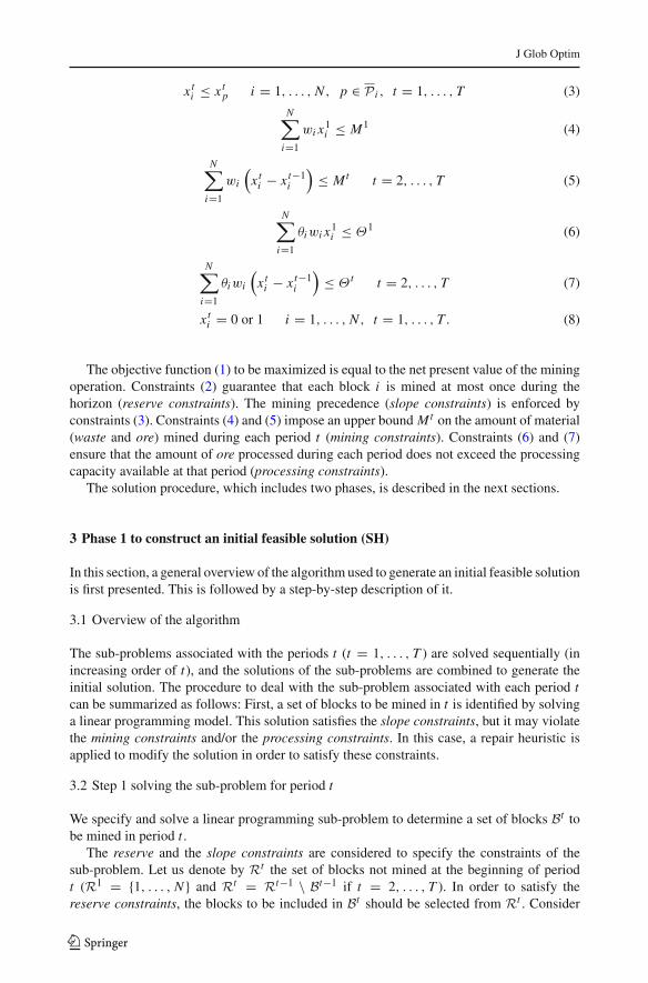
– N 1 (Exchange): Let i and j be two blocks mined in periods t and (t +1), respectively. Anexchange consists of replacing Bt and Bt+1 by (Bt − {i}) + { j} and (Bt+1 − { j}) + {i},respectively. The exchange of two blocks is feasible if the resulting solution is feasible;i.e., only if it satisfies the slope, the mining, and the processing constraints. Figure 2 givesa 2-dimensional illustration of an exchange move involving two blocks, i and j , withT = 2.

– N 2 (Shift-after): Let i be a block mined in period t , and let I = {i}∪{block s : s ∈ Si ∩Bt }denote the set including i and its successors mined in the same period. A shift-after consists

i

j

i

jjj

Current solution x robhgieN solution x obtained by the exchange move

ii

j

i

jjj

Current solution x robhgieN solution x obtained by the exchange

i

Fig. 2 Exchange move between blocks i and j with T = 2. The grey area represents the set of blocks to bemined in the first period (B1), while the white area delimited by the thick lines represents the set of blocks tobe mined in period 2 (B2)

123

J Glob Optim

Current solution x Neighbor solution x obtained by the Shift-after move

i and its succesors mined in period 1

Fig. 3 Shift-after move of block i and its successors mined in the same period. The grey area represents theset of blocks to be mined in the first period (B1), while the white area delimited by the thick lines representsthe set of blocks to be mined in period 2 (B2)

Current solution x Neighbor solution x obtained by the Shift-before move

i and its predecessors mined in period 2

Current solution x Neighbor solution x obtained by the Shift-before

i and its predecessors mined in period 2

Fig. 4 Shift-before move of block i and its predecessors mined in the same period. The grey area representsthe set of blocks to be mined in the first period (B1), while the white area delimited by the thick lines representsthe set of blocks to be mined in period 2 (B2)

of replacing Bt and Bt+1 by Bt −I and Bt+1+I, respectively. Clearly, the slope constraintsare satisfied in the resulting solution since the blocks are moved along with their successors.However, the mining and the processing constraints must be satisfied in period (t + 1) inorder to allow this shift-after. Figure 3 illustrates the Shift-after move where block i andits successors mined in period 1 are moved to period 2.

– N 3 (Shift-before): Let i be a block mined in period t , and let I = {i} ∪ {block p : p ∈Pi ∩Bt } denote the set including i and its predecessors mined in the same period. A shift-before consists of replacing Bt and Bt−1 by Bt − I and Bt−1 + I, respectively. As for theShift-after neighborhood, the slope constraints are necessarily satisfied, but the miningand the processing constraints in period (t − 1) must be satisfied in order to allow thisshift-before. Figure 4 illustrates the Shift-before move where block i and its predecessorsmined in period 2 are moved to period 1.

The strategy to explore any of the three neighborhoods is as follows: Consider the firstneighborhood N 1. Periods t = 1, . . . , (T −1) are considered sequentially in increasing order.Given a period t , all feasible exchanges involving pairs of blocks mined in t and (t + 1) aresystematically considered. The best exchange is selected. We apply the selected exchange ifit leads to a better solution or to a solution of the same value as the current solution (in order

123

J Glob Optim

to escape from the current local optimum). The process is iterated with the new solution.When no feasible exchange exists to further improve the solution or to get a solution of equalvalue, the next period (t + 1) is considered; i.e., exchanges involving pairs of blocks minedin periods (t + 1) and (t + 2) are evaluated.

The same exploration strategy is used when considering the Shift-after neighborhood N 2

except that periods t = 1, . . . , (T −1) are considered in decreasing order. For the Shift-beforeneighborhood N 3, periods t = 2, . . . , T are considered in increasing order.

4.2 Variable neighborhood descent procedure

The rules of a basic VND are applied: Start by exploring the Exchange neighborhood (N 1).When the search of N 1 is completed (i.e., for all t = 1, . . . , (T − 1), no feasible exchangebetween pairs of blocks mined in periods t and (t + 1) exists to further improve the solutionor to get a solution of equal value), restart a new search using the Shift-after neighborhood(N 2). Once the search of N 2 is completed, if the solution has been improved, return to N 1;otherwise, use the Shift-before neighborhood (N 3). This process terminates when no movein any of the three neighborhoods improves the value of the objective function.

Note that the Shift-after neighborhood (N 2) is explored before the Shift-before neighbor-hood (N 3) to create an opportunity for other blocks to be added to a given period t withoutexceeding the mining and the processing capacities available at t . Indeed, by first movingblocks from period 1 to period 2 (last shifts using N 2), more capacity becomes available inperiod 1 to include other blocks from period 2 (first shifts using N 3).

5 Numerical results

The method described in this paper is tested on instances generated from actual mineraldeposits, as well as on benchmark instances from the literature. All numerical experimentswere performed on an Intel(R) Xeon(R) CPU E7-8837 computer (2.67 GHz) with 1 TB ofRAM running under Linux. Before reporting the numerical results, we first introduce theinstances and the parameters used in the experiments.

5.1 Test instances

5.1.1 Instances generated from actual mineral deposits

Two different sets of instances, P1 and P2, are used. Instances in P1 and P2 are generated froman actual copper deposit where blocks i are of size 20×20×10 meters and weighwi = 10, 800tons each, and from an actual gold deposit where blocks i are of size 15 × 15 × 10 metersand weigh wi = 5, 625 tons each, respectively. The economic parameters used to computethe blocks’ economic values vi are also based on real-life data, and they are summarized inTable 1.

Each set (P1 and P2) includes 5 different instances characterized by a number of blocks Nand a number of periods T , specified in Table 2. The 10 instances have been constructed byvarying (perturbing) the blocks’ economic values vi . More precisely, to generate a specificinstance, the profit associated with each block i in the mineral deposit (i = 1, . . . , N ) isobtained by reducing vi by a factor D. Then, the following mathematical model is solvedto determine the pit limits; i.e., to identify the set of blocks maximizing the total profit butaccounting only for the slope constraints:

123

J Glob Optim

Table 1 Economic parameters Parameters P1 P2

Mining cost $1/t $1/t

Processing cost $9/t $15/t

Metal price $2/lb $900/oz

Selling cost $0.3/lb $7/oz

Discount rate 10 % 10 %

Table 2 Characteristics of the 10 instances generated from actual mineral deposits

Set Instance D Number ofblocks (N )

Number ofperiods (T )

P1 C1 20,000 4,273 3

Metal type: copper C2 15,000 7,141 4

Block size: 20 × 20 × 10 m C3 10,000 12,627 7

Block weight: wi = 10,800 tons C4 5,000 20,626 10

C5 0 26, 021 13

P2 G1 20,000 18,821 5

Metal type: gold G2 15,000 23,901 7

Block size: 15 × 15 × 10 m G3 10,000 30,013 8

Block weight: wi = 5,625 tons G4 5,000 34,981 9

G5 0 40,762 11

maxN∑

i=1

(vi − D)yi (14)

(P L D) Subject to

yi ≤ yp i = 1, . . . , N , p ∈ P i (15)

yi = 0 or 1 i = 1, . . . , N . (16)

Referring to an optimal solution y∗ of (P L D), N = |{block i : y∗i = 1}|. Note that N

decreases with the factor D. Each period is one year long. The number of periods is set to

T = ∑N

i=1 wi22.3M (M = million).

For each of the 10 instances, the production capacities are identical in all periodsand emulate those in real-world problems. For each period t , the mining capacity W t

is set to 1.25∑N

i=1 wiT and 1.30

∑Ni=1 wiT for instances in P1 and P2, respectively (i.e.,

total amount of rocknumber of periods plus a margin of 25 % and 30 %, respectively). The processing capacity

Θ t is set to 1.05∑N

i=1 wi θiT

(i.e, total amount of ore

number of periods plus a margin of 5 %)

.

5.1.2 First set of benchmark instances

As mentioned in the introduction, recent methods for solving the open-pit mine productionscheduling problem (MPSP) have been proposed by Amaya et al. [1], Moreno et al. [22],and Chicoisne et al. [11]. These methods have been applied to a set of four instances. In ourexperiments, we use two of these four instances; namely, AmericaMine and Marvin. Notethat Marvin is also used in the studies by Bienstock and Zuckerberg [3] and Cullenbine et

123

J Glob Optim

Table 3 Characteristics of the two instances in the first set of benchmark instances

Instance Number of blocks (N ) Number of periods (T )

AmericaMine 19,320 15

Metal type: polymetalic (not specified by the authors)

Block size: Unknown

Block weight wi : variable

Marvin 53,668 15

Metal type: copper and gold

Block size: 30 × 30 × 30 m


al. [12]. We don’t use the other two instances (AsiaMine and Andina) because they were notavailable in the public domain (due to confidentiality considerations).

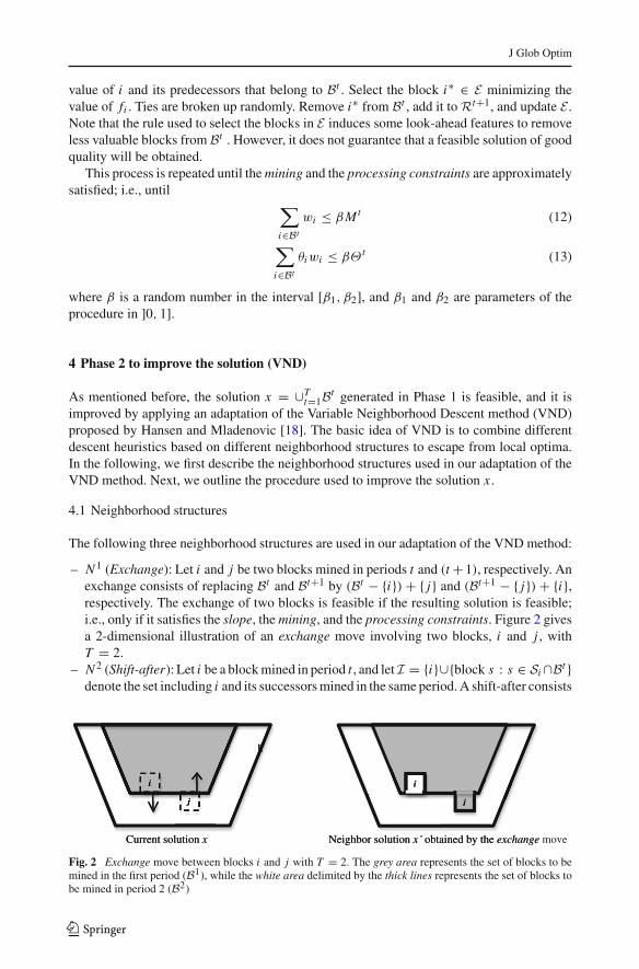
The characteristics of the two instances considered in this paper are as follows and aresummarized in Table 3: AmericaMine is a hard rock polymetalic mine containing 19,320blocks, while Marvin is a fictitious copper and gold orebody, included in Whittle [28], andhas 53,668 blocks (Whittle is a commercial mine planning software commonly used by pro-fessional mine planners). In both instances, blocks have different weights and are scheduledover 15 years. The production capacities are identical in all years. For AmericaMine, themining capacity W t is equal to 1M and the processing capacity Θ t is equal to 0.55M (M =million). For Marvin, W t = 60M and Θ t = 20M .

5.1.3 Second set of benchmark instances: MineLib test instances

The last dataset on which the method proposed in this paper is tested consists of instancesfrom MineLib, a library of publicly available test problem instances proposed by Espinoza etal. [15] for three classical types of open pit mining problems. The authors refer to the variantof the open-pit mine production scheduling problem, denoted in this paper by MPSP, as theconstrained pit limit problem, and they denote it by CPIT. They provide 11 instances wherethe number of operational resource constraints ranges from 1 to 3, and they are related tothe total amount extracted and/or the total amount processed in one or two different mills.In 3 of these 11 instances (namely, D, McLaughlin Limit, and McLaughlin) data related tothe weight of the blocks (wi ) is only available for ore blocks (i.e., data is missing for wasteblocks). Therefore, the method described in Sect. 3 cannot be applied to generate the initialsolution for these instances ( recall that this method is based on the value per unit of weight ofeach block; i.e., vi

wi). Hence, these instances are not used in our experiments, and we consider

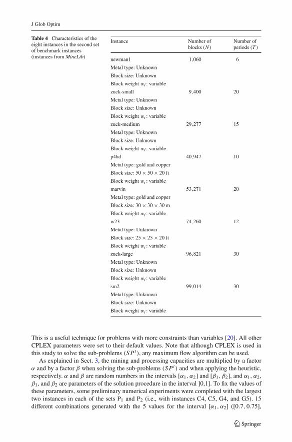
only the 8 other instances in MineLib. Table 4 reports the size of each of these 8 instances;their other characteristics can be found at http://mansci.uai.cl/minelib. Note that the instance“marvin in Table 4 is different from the instance “marvin” in Table 3 as far as the number ofblocks (N ) and the number of periods (T ) are concerned.

5.2 Parameter calibration

Version 12.5 of the commercial solver CPLEX was used to solve the sub-problems (S Pt );i.e., the mathematical model (9)–(11) introduced in Sect. 3.2. The predual parameter ofCPLEX was set to 1; that is, the dual linear programming problem is passed to the optimizer.

123

http://mansci.uai.cl/minelib

J Glob Optim

Table 4 Characteristics of theeight instances in the second setof benchmark instances(instances from MineLib)

Instance Number ofblocks (N )

Number ofperiods (T )

newman1 1,060 6

Metal type: Unknown

Block size: Unknown


zuck-small 9,400 20

Metal type: Unknown

Block size: Unknown


zuck-medium 29,277 15

Metal type: Unknown

Block size: Unknown


p4hd 40,947 10

Metal type: gold and copper

Block size: 50 × 50 × 20 ft


marvin 53,271 20

Metal type: gold and copper

Block size: 30 × 30 × 30 m


w23 74,260 12

Metal type: Unknown

Block size: 25 × 25 × 20 ft


zuck-large 96,821 30

Metal type: Unknown

Block size: Unknown


sm2 99,014 30

Metal type: Unknown

Block size: Unknown


This is a useful technique for problems with more constraints than variables [20]. All otherCPLEX parameters were set to their default values. Note that although CPLEX is used inthis study to solve the sub-problems (S Pt ), any maximum flow algorithm can be used.

As explained in Sect. 3, the mining and processing capacities are multiplied by a factorα and by a factor β when solving the sub-problems (S Pt ) and when applying the heuristic,respectively. α and β are random numbers in the intervals [α1, α2] and [β1, β2], and α1, α2,β1, and β2 are parameters of the solution procedure in the interval ]0,1]. To fix the values ofthese parameters, some preliminary numerical experiments were completed with the largesttwo instances in each of the sets P1 and P2 (i.e., with instances C4, C5, G4, and G5). 15different combinations generated with the 5 values for the interval [α1, α2] ([0.7, 0.75],

123

J Glob Optim

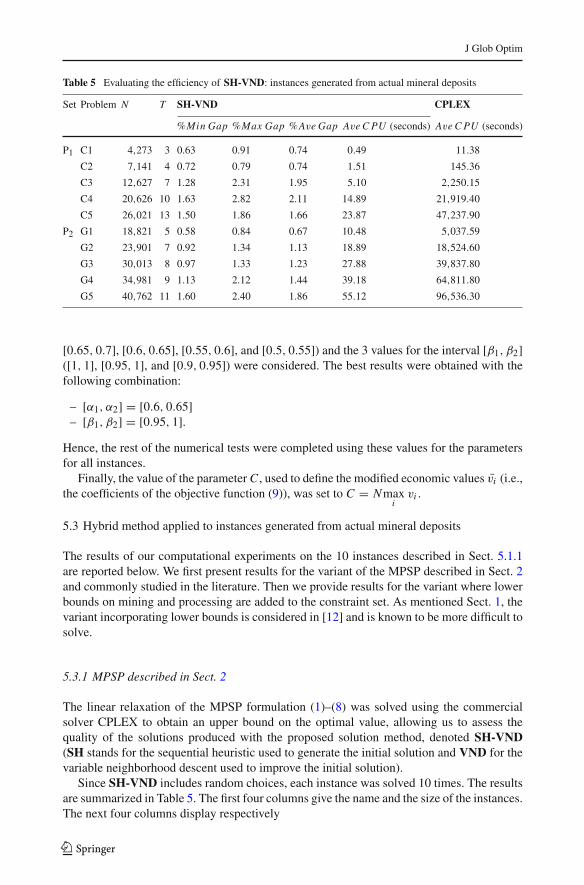
Table 5 Evaluating the efficiency of SH-VND: instances generated from actual mineral deposits

Set Problem N T SH-VND CPLEX

%Min Gap %Max Gap %Ave Gap Ave C PU (seconds) Ave C PU (seconds)

P1 C1 4,273 3 0.63 0.91 0.74 0.49 11.38

C2 7,141 4 0.72 0.79 0.74 1.51 145.36

C3 12,627 7 1.28 2.31 1.95 5.10 2,250.15

C4 20,626 10 1.63 2.82 2.11 14.89 21,919.40

C5 26,021 13 1.50 1.86 1.66 23.87 47,237.90

P2 G1 18,821 5 0.58 0.84 0.67 10.48 5,037.59

G2 23,901 7 0.92 1.34 1.13 18.89 18,524.60

G3 30,013 8 0.97 1.33 1.23 27.88 39,837.80

G4 34,981 9 1.13 2.12 1.44 39.18 64,811.80

G5 40,762 11 1.60 2.40 1.86 55.12 96,536.30

[0.65, 0.7], [0.6, 0.65], [0.55, 0.6], and [0.5, 0.55]) and the 3 values for the interval [β1, β2]([1, 1], [0.95, 1], and [0.9, 0.95]) were considered. The best results were obtained with thefollowing combination:

– [α1, α2] = [0.6, 0.65]– [β1, β2] = [0.95, 1].

Hence, the rest of the numerical tests were completed using these values for the parametersfor all instances.

Finally, the value of the parameter C , used to define the modified economic values v̄i (i.e.,the coefficients of the objective function (9)), was set to C = Nmax

ivi .

5.3 Hybrid method applied to instances generated from actual mineral deposits

The results of our computational experiments on the 10 instances described in Sect. 5.1.1are reported below. We first present results for the variant of the MPSP described in Sect. 2and commonly studied in the literature. Then we provide results for the variant where lowerbounds on mining and processing are added to the constraint set. As mentioned Sect. 1, thevariant incorporating lower bounds is considered in [12] and is known to be more difficult tosolve.

5.3.1 MPSP described in Sect. 2

The linear relaxation of the MPSP formulation (1)–(8) was solved using the commercialsolver CPLEX to obtain an upper bound on the optimal value, allowing us to assess thequality of the solutions produced with the proposed solution method, denoted SH-VND(SH stands for the sequential heuristic used to generate the initial solution and VND for thevariable neighborhood descent used to improve the initial solution).

Since SH-VND includes random choices, each instance was solved 10 times. The resultsare summarized in Table 5. The first four columns give the name and the size of the instances.The next four columns display respectively

123

J Glob Optim

– %Min Gap = ZL R−ZbestZL R

× 100: the value of the relative gap between the value Zbest ofthe best solution obtained by SH-VND over the 10 runs and the optimal value ZL R ofthe linear relaxation.

– %Max Gap = ZL R−ZworstZL R

× 100: the value of the relative gap between the value Zworst

of the worst solution obtained by SH-VND over the 10 runs and the optimal value of thelinear relaxation.

– %Ave Gap = ZL R−ZaverageZL R

× 100: the value of the relative gap between the averagevalue Zaverage of the 10 solutions generated by SH-VND and the optimal value of thelinear relaxation.

– Ave C PU : the average solution time in seconds.

The last column of Table 5 indicates the CPU time required by CPLEX to solve the linearrelaxation of the problems. Note that the length of the interval [%Min Gap, %Max Gap]indicates the robustness of the proposed method with respect to random choices. The follow-ing observations can be derived from Table 5:

– SH-VND is very efficient in the sense that for each problem the value of %Min Gapis less than 2 % away from the upper bound provided by CPLEX. This indicates that atleast one of the 10 solutions generated is of excellent quality. Even though 10 runs arerequired to achieve this %Min Gap, this is acceptable since the CPU time of a run isless than 1 min for all the tested instances.

– SH-VND is very robust in the sense that in all cases (considering the 10 instances andthe 10 runs) the gap between the solution generated and the upper bound provided byCPLEX is smaller than 3 %, and in 92 % of all cases, it is smaller than 2 % (cf. values of%Max Gap).

– The time required to find these high quality solutions is very reasonable. For the smallestproblem, C1, a near-optimal solution is found almost immediately (less than 1 s). For thelargest problem, G5, the CPU time is less than 1 min.

– As expected, the solution time increases with the number of blocks in the instance, butthe rate of increase is larger for CPLEX than for SH-VND. Indeed, CPLEX may requiremore than 1 day (almost 27 h) to solve the linear relaxation of the largest problem, G5,while a very good feasible solution for this problem is obtained in less than 1 min bySH-VND.

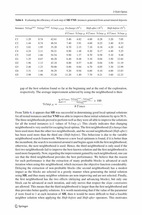
Next the performance of SH-VND is investigated in more detail. Table 6 shows theimprovement gained at each step of the algorithm. For each instance, we first give %Gapinit ,the gap of the initial solution computed as the relative difference between the value of thisinitial solution, obtained using the sequential heuristic (SH) described in Sect. 3, and theoptimal value of the linear relaxation. This is followed by %Gap f inal , the gap of the finalsolution obtained after applying the VND procedure described in Sect. 4, and %I mp.V N D =%Gapinit −%Gap f inal

%Gapinit × 100 as a measure of the improvement achieved by using VND. Note

that the three measures above (%Gapinit , %Gap f inal , and %I mp.V N D) are averaged overthe 10 runs and hence %Gap f inal corresponds to %Ave Gap in Table 5. We then report foreach of the three neighborhood structures, used in our adaptation of VND, the two followingmeasures also averaged over the 10 runs:

– # T imes: the number of times that the neighborhood has been explored– %I mp.N : the average improvement in percent gained by using the neighborhood. To

compute the value of %I mp.N , we proceed as follows: Suppose that the neighborhoodis explored for the kth time (k = 1, . . . , # T imes). Let %Gapstart

k and %Gapendk be the

123

J Glob Optim

Table 6 Evaluating the efficiency of each step of SH-VND: instances generated from actual mineral deposits

Instance %Gapinit %Gap f inal %I mp.V N D Exchange (N 1) Shift-after (N 2) Shift-before (N 3)

# T imes %I mp.N # T imes %I mp.N # T imes %I mp.N

C1 1.29 0.74 42.61 5.40 4.82 4.00 0.28 3.20 7.05

C2 1.44 0.74 48.54 7.40 3.91 4.60 0.25 3.40 8.53

C3 3.01 1.95 35.20 8.70 2.15 7.10 0.18 4.20 6.42

C4 4.24 2.11 50.21 8.90 1.48 8.20 0.17 4.40 5.25

C5 3.65 1.66 54.54 9.90 1.37 8.70 0.58 5.10 9.48

G1 1.25 0.67 46.28 6.40 0.48 5.10 0.04 3.50 12.84

G2 1.96 1.13 42.18 8.00 0.57 6.40 0.04 3.50 11.19

G3 2.46 1.23 50.08 8.80 0.84 6.70 0.05 3.30 12.99

G4 3.31 1.44 56.29 9.20 0.94 6.60 0.10 4.00 13.83

G5 3.98 1.86 53.28 11.20 1.40 7.70 0.21 3.60 12.23

gap of the best solution found so far at the beginning and at the end of the exploration,respectively. The average improvement achieved by using the neighborhood is then:

%I mp.N =∑# T imes

k=1%Gapstart

k −%Gapendk

%Gapstartk

× 100

# T imes.

From Table 6, it appears that SH was successful in determining good local optimal solutionsfor all tested instances and that VND was able to improve these initial solutions by up to 56 %.The three neighborhoods proved to perform well as they were all able to improve the solutionsfor all the tested instances (c.f. values of %I mp.N ). This clearly indicates that changingneighborhood is very useful for escaping local optima. The first neighborhood (Exchange) hasbeen used more than the other two neighborhoods, and the second neighborhood (Shift-after)has been used more than the third one (Shift-before). This behaviour is due to the variableneighborhood search framework: Whenever a new local optimum is found, if it is better thanthe incumbent, the search is recentered around it and begins again with the first neighborhood;otherwise, the next neighborhood is used. Hence, the third neighborhood is only used if thefirst two neighborhoods fail to improve the best-known solution and the first neighborhood isused more frequently. Now, regarding the improvement gained by each neighborhood, one cansee that the third neighborhood provides the best performance. We believe that the reasonfor such performance is that the extraction of many profitable blocks is advanced at eachiteration when using this neighborhood, which increases the objective function considerably.Delaying the extraction of non-profitable blocks (the second neighborhood) has a modestimpact as the blocks are selected in a greedy manner when generating the initial solutionusing SH, and thus many neighbor solutions are non-improving and are not selected. Finally,the first neighborhood has the two effects (delaying and advancing blocks), but only oneblock can be advanced at each iteration, and only moves that respect the slope constraintsare allowed. This means that the third neighborhood is larger than the first neighborhood andthus provides better quality solutions. It is worth mentioning that if the value of the parameterβ were fixed to 1 at each iteration of SH, then it would be more difficult to find a feasibleneighbor solution when applying the Shift-before and Shift-after operators. This motivates

123

J Glob Optim

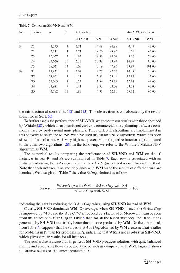
Table 7 Comparing SH-VND and WM

Set Instance N T %Ave Gap Ave C PU (seconds)

SH-VND WM %I mp. SH-VND WM

P1 C1 4,273 3 0.74 14.48 94.89 0.49 43.00

C2 7,141 4 0.74 18.26 95.95 1.51 64.00

C3 12,627 7 1.95 19.58 90.04 5.10 78.00

C4 20,626 10 2.11 20.98 89.94 14.89 85.00

C5 26,021 13 1.66 3.19 47.96 23.87 101.00

P2 G1 18,821 5 0.67 3.77 82.24 10.48 30.00

G2 23,901 7 1.13 5.51 79.49 18.89 57.00

G3 30,013 8 1.23 2.94 58.14 27.88 44.00

G4 34,981 9 1.44 2.33 38.08 39.18 63.00

G5 40,762 11 1.86 4.91 62.10 55.12 65.00

the introduction of constraints (12) and (13). This observation is corroborated by the resultspresented in Sect. 5.5.

To further assess the performance of SH-VND, we compare our results with those obtainedby Whittle [28], which is, as mentioned earlier, a commercial mine planning software com-monly used by professional mine planners. Three different algorithms are implemented inthis software to solve the MPSP. We have used the Milawa NPV algorithm, which has beenshown to find solutions with very high net present value (objective function (1)) comparedto the other two algorithms [28]. In the following, we refer to the Whittle’s Milawa NPValgorithm as WM.

The numerical results comparing the performance of SH-VND and WM on the 10instances in sets P1 and P2 are summarized in Table 7. Each row is associated with aninstance indicating the %Ave Gap and the Ave C PU (as defined above) for each method.Note that each instance is solved only once with WM since the results of different runs areidentical. We also give in Table 7 the value %I mp. defined as follows:

%I mp. = %Ave Gap with WM − %Ave Gap with SH

%Ave Gap with WM× 100

indicating the gain in reducing the %Ave Gap when using SH-VND instead of WM.Clearly, SH-VND dominates WM. On average, when SH-VND is used, the %Ave Gap

is improved by 74 %, and the Ave C PU is reduced by a factor of 3. Moreover, it can be seenfrom the values of %Max Gap in Table 5 that, for all the tested instances, the 10 solutionsgenerated by SH-VND are strictly better than the one produced by WM. On the other hand,from Table 7, it appears that the values of %Ave Gap obtained by WM are somewhat smallerfor problems in P2 than for problems in P1, indicating that WM is not as robust as SH-VND,which gives similar results for all instances.

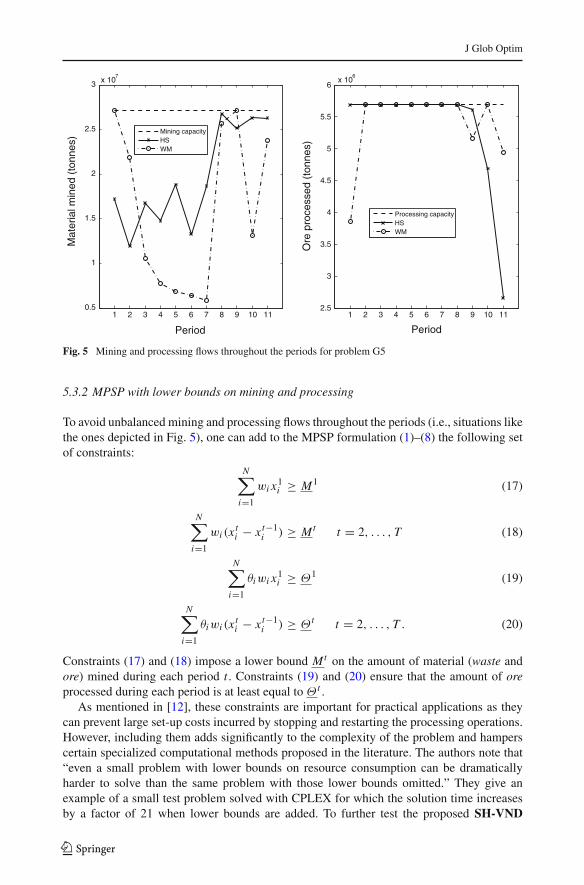
The results also indicate that, in general, SH-VND produces solutions with quite balancedmining and processing flows throughout the periods as compared with WM. Figure 5 showsillustrative results on the largest problem, G5.

123

J Glob Optim

1 2 3 4 5 6 7 8 9 10 110.5

1

1.5

2

2.5

3 x 107

Period

Mat

eria

l min

ed (

tonn

es)

1 2 3 4 5 6 7 8 9 10 112.5

3

3.5

4

4.5

5

5.5

6x 10

6

Period

Ore

pro

cess

ed (

tonn

es)

Processing capacityHSWM

Mining capacityHSWM

Fig. 5 Mining and processing flows throughout the periods for problem G5

5.3.2 MPSP with lower bounds on mining and processing

To avoid unbalanced mining and processing flows throughout the periods (i.e., situations likethe ones depicted in Fig. 5), one can add to the MPSP formulation (1)–(8) the following setof constraints:

N∑i=1

wi x1i ≥ M1 (17)

N∑i=1

wi (xti − xt−1

i ) ≥ Mt t = 2, . . . , T (18)

N∑i=1

θiwi x1i ≥ Θ1 (19)

N∑i=1

θiwi (xti − xt−1

i ) ≥ Θ t t = 2, . . . , T . (20)

Constraints (17) and (18) impose a lower bound Mt on the amount of material (waste andore) mined during each period t . Constraints (19) and (20) ensure that the amount of oreprocessed during each period is at least equal to Θ t .

As mentioned in [12], these constraints are important for practical applications as theycan prevent large set-up costs incurred by stopping and restarting the processing operations.However, including them adds significantly to the complexity of the problem and hamperscertain specialized computational methods proposed in the literature. The authors note that“even a small problem with lower bounds on resource consumption can be dramaticallyharder to solve than the same problem with those lower bounds omitted.” They give anexample of a small test problem solved with CPLEX for which the solution time increasesby a factor of 21 when lower bounds are added. To further test the proposed SH-VND

123

J Glob Optim

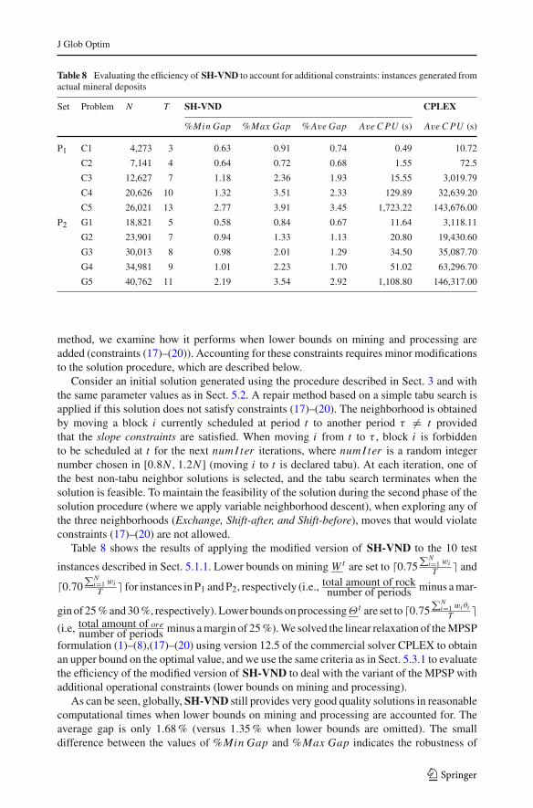
Table 8 Evaluating the efficiency of SH-VND to account for additional constraints: instances generated fromactual mineral deposits

Set Problem N T SH-VND CPLEX

%Min Gap %Max Gap %Ave Gap Ave C PU (s) Ave C PU (s)

P1 C1 4,273 3 0.63 0.91 0.74 0.49 10.72

C2 7,141 4 0.64 0.72 0.68 1.55 72.5

C3 12,627 7 1.18 2.36 1.93 15.55 3,019.79

C4 20,626 10 1.32 3.51 2.33 129.89 32,639.20

C5 26,021 13 2.77 3.91 3.45 1,723.22 143,676.00

P2 G1 18,821 5 0.58 0.84 0.67 11.64 3,118.11

G2 23,901 7 0.94 1.33 1.13 20.80 19,430.60

G3 30,013 8 0.98 2.01 1.29 34.50 35,087.70

G4 34,981 9 1.01 2.23 1.70 51.02 63,296.70

G5 40,762 11 2.19 3.54 2.92 1,108.80 146,317.00

method, we examine how it performs when lower bounds on mining and processing areadded (constraints (17)–(20)). Accounting for these constraints requires minor modificationsto the solution procedure, which are described below.

Consider an initial solution generated using the procedure described in Sect. 3 and withthe same parameter values as in Sect. 5.2. A repair method based on a simple tabu search isapplied if this solution does not satisfy constraints (17)–(20). The neighborhood is obtainedby moving a block i currently scheduled at period t to another period τ �= t providedthat the slope constraints are satisfied. When moving i from t to τ , block i is forbiddento be scheduled at t for the next num I ter iterations, where num I ter is a random integernumber chosen in [0.8N , 1.2N ] (moving i to t is declared tabu). At each iteration, one ofthe best non-tabu neighbor solutions is selected, and the tabu search terminates when thesolution is feasible. To maintain the feasibility of the solution during the second phase of thesolution procedure (where we apply variable neighborhood descent), when exploring any ofthe three neighborhoods (Exchange, Shift-after, and Shift-before), moves that would violateconstraints (17)–(20) are not allowed.

Table 8 shows the results of applying the modified version of SH-VND to the 10 test

instances described in Sect. 5.1.1. Lower bounds on mining W t are set to 0.75∑N

i=1 wiT and

0.70∑N

i=1 wiT for instances in P1 and P2, respectively (i.e., total amount of rock

number of periods minus a mar-

gin of 25 % and 30 %, respectively). Lower bounds on processingΘ t are set to 0.75∑N

i=1 wi θiT

(i.e, total amount of orenumber of periods minus a margin of 25 %). We solved the linear relaxation of the MPSP

formulation (1)–(8),(17)–(20) using version 12.5 of the commercial solver CPLEX to obtainan upper bound on the optimal value, and we use the same criteria as in Sect. 5.3.1 to evaluatethe efficiency of the modified version of SH-VND to deal with the variant of the MPSP withadditional operational constraints (lower bounds on mining and processing).

As can be seen, globally, SH-VND still provides very good quality solutions in reasonablecomputational times when lower bounds on mining and processing are accounted for. Theaverage gap is only 1.68 % (versus 1.35 % when lower bounds are omitted). The smalldifference between the values of %Min Gap and %Max Gap indicates the robustness of

123

J Glob Optim

0 1 2 3 4 5 6 7 8 9 10 110.5

1

1.5

2

2.5

3x 10

7

Period

Mat

eria

l min

ed (

tonn

es)

0 1 2 3 4 5 6 7 8 9 10 11 122.5

3

3.5

4

4.5

5

5.5

6x 10

6

Period

Ore

pro

cess

ed (

tonn

es)

Lower bound on processing

Upper bound on processing

Amount processed

Lower bound on mining

Upper bound on mining

Amount mined

Fig. 6 Mining and processing flows throughout the periods for problem G5 when lower bounds are added

SH-VND. Overall, solution times tend to remain reasonable. We observe that for instancesC1, C2, G1, and G2, adding lower bounds does not affect the solution time (CPU times arecomparable to those when lower bounds are omitted, c.f. Table 5). For these instances, theinitial solutions generated were actually in most of the runs feasible, so the repair heuristic(tabu search) was not necessary. However, for the other instances, the solutions times arelonger because it is hard to find a feasible solution. For the largest problem in the set P1, C5,the bounds are very tight, and typically about 80 % of the CPU time is spent in looking fora feasible solution. Although the solution times required by SH-VND are longer when weaccount for the lower bounds constraints than when we don’t (range between 1 s and 29 minversus 1 s and 1 min), they are still significantly smaller than those required by CPLEX tosolve the linear relaxation of the problem. For instance, for the largest instance G5, CPLEXrequires almost 2 days to solve the linear relaxation of the problem, while SH-VND canfind a near-optimal solution in only about 18 min on average. Figure 6 shows the mining andprocessing flows throughout the periods for this problem in a solution generated by SH-VND.

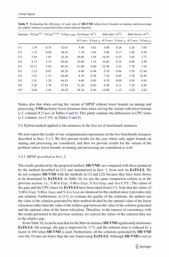
Next, Table 9 presents detailed results allowing us to analyze the efficiency of each stepof the proposed algorithm. This table has the same structure as Table 6. Similar conclusions,as in solving the variant without lower bounds on mining and processing, are obtained:

– For each instance, except C5, the initial solutions are of very good quality, within lessthan 5 % of optimality

– VND was able to improve the initial solutions by more than 50 % on average– The three neighborhoods perform well as they all improve the solutions for all the tested

instances– The Shift-before (N 2) neighborhood is again the best one; that is, the one that improves

the most the solution– The Shift-after (N 3) neighborhood is not competitive although it performs slightly better

than when solving the variant where the lower bounds are omitted, especially for thelargest problems, C5 and G5, which are much harder to solve.

123

J Glob Optim

Table 9 Evaluating the efficiency of each step of SH-VND when lower bounds on mining and processingare added: instances generated from actual mineral deposits

Instance %Gapinit %Gap f inal %I mp.VND Exchange (N 1) Shift-after (N 2) Shift-before (N 3)


C1 1.29 0.74 42.61 5.40 4.82 4.00 0.28 3.20 7.05

C2 1.32 0.68 48.42 7.70 3.69 5.00 0.17 3.40 8.59

C3 2.94 1.93 34.28 20.80 1.05 18.50 0.25 3.60 3.77

C4 4.72 2.33 50.64 14.80 1.14 16.00 0.24 4.90 2.89

C5 10.31 3.45 66.54 21.00 0.69 22.50 2.23 7.70 1.92

G1 1.25 0.67 46.28 6.40 0.48 5.10 0.04 3.50 12.84

G2 1.91 1.13 40.88 8.10 0.58 7.10 0.05 3.70 10.56

G3 2.41 1.29 46.43 9.60 0.85 9.70 0.09 4.50 8.84

G4 3.26 1.70 47.84 12.20 0.85 9.50 0.11 7.20 6.96

G5 4.60 2.92 36.59 18.30 0.46 19.90 1.15 4.20 2.02

Notice also that when solving the variant of MPSP without lower bounds on mining andprocessing, VND performs fewer iterations than when solving the variant with lower bounds(c.f. columns # T imes in Tables 6 and 9). This partly explains the differences in CPU times(c.f. columns Ave C PU in Tables 5 and 8).

5.4 Hybrid method applied to the instances in the first set of benchmark instances

We now report the results of our computational experiments on the two benchmark instancesdescribed in Sect. 5.1.2. We first present results for the case where only upper bounds onmining and processing are considered, and then we provide results for the variant of theproblem where lower bounds on mining and processing are considered as well.

5.4.1 MPSP described in Sect. 2

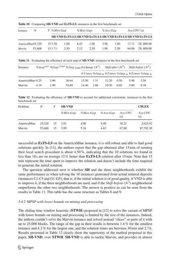
The results produced by the proposed method, SH-VND, are compared with those producedby the method described in [11] and summarized in Sect. 1, from now on ExTS-LS. Wedo not compare SH-VND with the methods in [1] and [22] because they have been shownto be dominated by ExTS-LS. In Table 10, we use the same comparison criteria as in theprevious section; i.e., %Min Gap, %Max Gap, %Ave Gap, and Ave C PU . The values ofthe gaps and the CPU times for ExTS-LS have been taken from [11]. Note that the values of%Min Gap, %Max Gap, and %Ave Gap are identical for this method since it provides onlyone solution. Furthermore, in [11], to evaluate the quality of the solutions, the authors usethe value of the solution generated by their method divided by the optimal value of the linearrelaxation rather than the value of the relative gap between the value of the solution generatedand the optimal value of the linear relaxation. Therefore, in the interest of consistency withthe results presented in the previous sections, we convert the values of the criterion they useto the relative gap.

From Table 10, it can be seen that for the Marvin instance SH-VND significantly dominatesExTS-LS. On average, the gap is improved by 17 % and the solution time is reduced by afactor of 450 when SH-VND is used. Furthermore, all the solutions generated by SH-VNDover the 10 runs are better than the one found using ExTS-LS. Although SH-VND is not as

123

J Glob Optim

Table 10 Comparing SH-VND and ExTS-LS: instances in the first benchmark set

Instance N T %Min Gap %Max Gap %Ave Gap Ave CPU (s)

SH-VND ExTS-LS SH-VND ExTS-LS SH-VND ExTS-LS SH-VND ExTS-LS

AmericaMine19,320 15 3.56 1.00 4.43 1.00 3.96 1.00 17.71 28, 800.00

Marvin 53,668 15 1.71 2.30 2.12 2.30 1.90 2.30 64.06 28, 800.00

Table 11 Evaluating the efficiency of each step of SH-VND: instances in the first benchmark set



AmericaMine 6.25 3.96 36.64 15.50 1.31 12.20 0.50 5.90 3.50

Marvin 4.19 1.90 54.69 14.40 1.66 10.50 0.02 5.00 8.38

Table 12 Evaluating the efficiency of SH-VND to account for additional constraints: instances in the firstbenchmark set

Problem N T SH-VND CPLEX

%Min Gap %Max Gap %Ave Gap Ave CPU(s)

Ave CPU(s)

AmericaMine 19,320 15 3.91 4.80 4.40 18.21 2,624.42

Marvin 53,668 15 3.99 5.34 4.63 67.00 97,702.30

successful as ExTS-LS on the AmericaMine instance, it is still robust and able to find goodsolutions quickly. In [11], the authors report that the gap obtained after 15 min of runningtheir local search procedure is about 4.50 %, indicating that the 10 solutions we found inless than 18 s are on average 12 % better than ExTS-LS solution after 15 min. Note that 15min represent the time spent to improve the solution and doesn’t include the time requiredto generate the initial solution.

The question addressed next is whether SH and the three neighborhoods exhibit thesame performance as when solving the 10 instances generated from actual mineral deposits(instances C1-C5 and G1-G5); that is, if the initial solution is of good quality, if VND is ableto improve it, if the three neighborhoods are used, and if the Shift-before (N 3) neighborhoodoutperforms the other two neighborhoods. The answer is positive as can be seen from theresults in Table 11. This table has the same structure as Tables 6 and 9.

5.4.2 MPSP with lower bounds on mining and processing

The sliding time window heuristic (STWH) proposed in [12] to solve the variant of MPSPwith lower bounds on mining and processing is limited by the size of the instances. Indeed,the authors couldn’t solve the Marvin instance and solved instead “slices” or parts of it withup to 25,000 blocks. The range of the gap in their results is between 1.4 % for the smallestinstance and 4.3 % for the largest one, and the solution times are between 30 min and 2.7 h.Results presented in Table 12 clearly show the superiority of the method proposed in thispaper, SH-VND, over STWH. SH-VND is able to tackle Marvin, and provides in almost

123

J Glob Optim

Table 13 Evaluating the efficiency of each step of SH-VND when solving the instances in the first benchmarkset with lower bounds on mining and processing



AmericaMine 6.47 4.40 32.05 14.40 1.03 13.70 0.47 5.70 2.71

Marvin 5.78 4.63 19.75 17.30 0.83 17.80 0.02 4.90 1.44

Table 14 Testing SH-VND on instances from MineLib

Instance N T %Ave Gap Best K nown Gap Ave C PU (s)SH-VND LR+Modified TopoSort SH-VND

newman1 1,060 6 1.68 4.10 0.08

zuck-small 9,400 20 1.80 7.70 7.77

zuck-medium 29,277 15 8.08 13.40 121.60

p4hd 40,947 10 6.61 0.50 78.57

marvin 53,271 20 1.87 5.00 70.74

w23 74,260 12 9.96 2.10 203.46

zuck-large 96,821 30 8.07 1.10 1,003.97

sm2 99,014 30 5.85 0.20 105.00

1 min very good solutions with an average gap of 4.63 %. Regarding the efficiency of the stepsof SH-VND, results reported in Table 13 indicate that each step of the algorithm performssimilarly as in the experiments discussed in the previous sections: good initial solutions withSH, improved significantly by VND, and the largest improvement are obtained with the thirdneighborhood, Shift-before.

5.5 Hybrid method applied to the instances in the second set of benchmark instances(instances from MineLib)

As mentioned earlier in Sect. 5.1.3, the method proposed in this paper, SH-VND, was alsocompared on instances from MineLib. The results are given in Table 14. We first recall in thefirst three columns the name of the instances and their sizes. Then, we give the %Ave Gap,as defined earlier (the value of the relative gap between the average value Zaverage of the10 solutions generated by SH-VND and the optimal value of the linear relaxation). Thistime, the optimal value of the linear relaxation has not been obtained using CPLEX, but ithas been taken from [15]. The authors mention that it has been computed using a modifiedversion of Bienstock-Zuckerberg’s algorithm [3]. The criterion %Ave Gap is followed byBest K nown Gap, the value of the gap of the current best-known integer-feasible solutioncomputed as the relative difference between the value of this feasible solution and the optimalvalue of the linear relaxation. The values of Best K nown Gap are also taken from [15]. Theauthors report that the current best-known integer-feasible solution has been obtained from theLP relaxation using a modified version of the TopoSort heuristic. The CPU time (in seconds)required by SH-VND to solve each instance is given in the last column of the table. We do notreport the CPU times of the method used to obtain the current best-known solutions becausethey are provided neither in [15] nor in http://mansci.uai.cl/minelib. Finally, when comparing

123


J Glob Optim

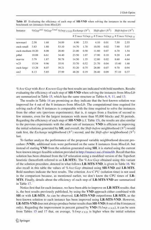
Table 15 Evaluating the efficiency of each step of SH-VND when solving the instances in the secondbenchmark set (instances from MineLib)



newman1 2.58 1.68 34.89 8.90 2.53 4.10 0.01 7.50 2.55

zuck-small 3.83 1.80 53.10 14.70 1.70 10.50 0.02 7.90 5.07

zuck-medium 10.20 8.08 20.80 21.00 0.58 11.80 0.07 6.70 1.54

p4hd 10.08 6.61 34.40 23.50 1.07 17.90 0.10 9.20 1.49

marvin 3.79 1.87 50.78 14.50 1.35 12.80 0.02 8.60 4.64

w23 15.54 9.96 35.91 33.70 0.52 21.70 0.04 15.40 1.68

zuck-large 13.28 8.07 39.21 53.20 0.75 28.00 0.07 9.70 0.94

sm2 8.13 5.85 27.99 48.20 0.19 28.40 0.09 57.10 0.37

%Ave Gap with Best K nown Gap the best results are indicated with bold numbers. Resultsevaluating the efficiency of each step of SH-VND when solving the instances from MineLibare summarized in Table 15, which has the same structure as Tables 6, 9, 11, and 13.

The results in Table 14 are promising as they indicate that the best-known solution wasimproved for 4 out of the 8 instances from MineLib. The computational time required forsolving each of the 8 instances is comparable with the time required to solve the instancesfrom the other sets (previous experiments); that is, it ranges from a fraction of second tofew minutes, even for the largest instances with more than 95,000 blocks and 30 periods.Regarding the efficiency of each step of SH-VND (c.f. Table 15), the results are also similarto the previous experiments with the other sets of instances: VND is efficient in improvingthe initial solutions generated by SH, and overall, the Shift-before neighborhood (N 3) wouldrank first, the Exchange neighborhood (N 1) second, and the Shift-after neighborhood (N 2)last.

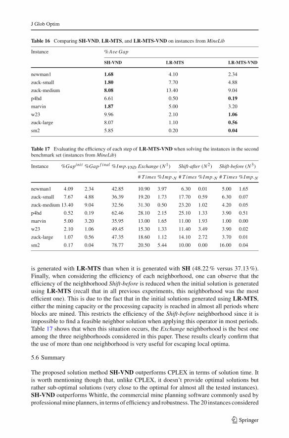
To further analyze the performance of the proposed variable neighborhood descent pro-cedure (VND), additional tests were performed on the same 8 instances from MineLib, butinstead of starting VND from the solution generated using SH, it is started using the currentbest-known integer-feasible solution provided in http://mansci.uai.cl/minelib. Recall that thissolution has been obtained from the LP relaxation using a modified version of the TopoSortheuristic (henceforth referred to as LR-MTS). The %Ave Gap obtained using this variantof the solution procedure, denoted in what follows LR-MTS-VND, is given in Table 16. Wealso recall in this table the values of %Ave Gap obtained using SH-VND and LR-MTS.Bold numbers indicate the best results. The criterion Ave C PU (solution time) is not usedin the comparison because, as mentioned earlier, we don’t know the CPU times of LR-MTS. Finally, details about the efficiency of each step of LR-MTS-VND are summarizedin Table 17.

Notice first that for each instance, we have been able to improve on LR-MTS results; thatis, the best results previously published, by using the VND approach either combined withSH or with LR-MTS. As can be observed, LR-MTS-VND outperforms LR-MTS, as thebest-known solution to each instance has been improved using LR-MTS-VND. However,LR-MTS-VND does not always produce better results than SH-VND (4 out of the 8 instancesonly). Regarding the improvement in percent gained by VND (%I mp.V N D), it can be seenfrom Tables 15 and 17 that, on average, %I mp.V N D is higher when the initial solution

123


J Glob Optim

Table 16 Comparing SH-VND, LR-MTS, and LR-MTS-VND on instances from MineLib

Instance %Ave Gap

SH-VND LR-MTS LR-MTS-VND

newman1 1.68 4.10 2.34

zuck-small 1.80 7.70 4.88

zuck-medium 8.08 13.40 9.04

p4hd 6.61 0.50 0.19

marvin 1.87 5.00 3.20

w23 9.96 2.10 1.06

zuck-large 8.07 1.10 0.56

sm2 5.85 0.20 0.04

Table 17 Evaluating the efficiency of each step of LR-MTS-VND when solving the instances in the secondbenchmark set (instances from MineLib)



newman1 4.09 2.34 42.85 10.90 3.97 6.30 0.01 5.00 1.65

zuck-small 7.67 4.88 36.39 19.20 1.73 17.70 0.59 6.30 0.07

zuck-medium 13.40 9.04 32.56 31.30 0.50 23.20 1.02 4.20 0.05

p4hd 0.52 0.19 62.46 28.10 2.15 25.10 1.33 3.90 0.51

marvin 5.00 3.20 35.95 13.00 1.65 11.00 1.93 1.00 0.00

w23 2.10 1.06 49.45 15.30 1.33 11.40 3.49 3.90 0.02

zuck-large 1.07 0.56 47.35 18.60 1.12 14.10 2.72 3.70 0.01

sm2 0.17 0.04 78.77 20.50 5.44 10.00 0.00 16.00 0.04

is generated with LR-MTS than when it is generated with SH (48.22 % versus 37.13 %).Finally, when considering the efficiency of each neighborhood, one can observe that theefficiency of the neighborhood Shift-before is reduced when the initial solution is generatedusing LR-MTS (recall that in all previous experiments, this neighborhood was the mostefficient one). This is due to the fact that in the initial solutions generated using LR-MTS,either the mining capacity or the processing capacity is reached in almost all periods whereblocks are mined. This restricts the efficiency of the Shift-before neighborhood since it isimpossible to find a feasible neighbor solution when applying this operator in most periods.Table 17 shows that when this situation occurs, the Exchange neighborhood is the best oneamong the three neighborhoods considered in this paper. These results clearly confirm thatthe use of more than one neighborhood is very useful for escaping local optima.

5.6 Summary

The proposed solution method SH-VND outperforms CPLEX in terms of solution time. Itis worth mentioning though that, unlike CPLEX, it doesn’t provide optimal solutions butrather sub-optimal solutions (very close to the optimal for almost all the tested instances).SH-VND outperforms Whittle, the commercial mine planning software commonly used byprofessional mine planners, in terms of efficiency and robustness. The 20 instances considered

123

J Glob Optim

in this paper were solved within less than 3.2 % of optimality, on average, in less than 2 min.When comparing SH-VND to recent solution methods proposed in the literature, the resultsindicate that it is better than the ExTS-LS method proposed by [11], providing an excellentcompromise between solution time and solution quality, as well as a new best-known solutionfor the instance Marvin. SH-VND and/or LR-MTS-VND also provide new best-knownsolutions for all the 8 instances from MineLib [15], indicating their superiority over the LR-MTS method. Another interesting feature of the proposed solution method is that it is not aspecialized method tailored to solve one variant of the open-pit mine production schedulingproblem, but it can be easily adapted to account for additional operational constraints. Wehave modified it to account for lower bounds on mining and processing. The results indicatethat although the average CPU time is higher than in the case when the lower bounds areomitted, the solution quality does not deteriorate when accounting for lower bounds. Onaverage, considering the 12 instances in which lower bounds on mining and processing wereadded, the gap is slightly above 2 % (2.15 %) and the solution time is only about 4 min. TheMarvin instance is intractable by the method proposed in [12], but it is successfully solvedby the method we have developed, SH-VND, indicating the superiority of SH-VND overthat method. Because SH-VND doesn’t rely on solving integer programming problems, itsrunning time has a slower growth rate compared to other solution methods in the literaturesuch as the ones in [11] and [12]. Indeed, the CPU time of SH-VND ranges between a fractionof second and 16 min for instances whose sizes vary from 1,060 blocks and 6 years to 99,014blocks and 30 periods.

6 Conclusions

Production scheduling is a challenging and critical issue for mining companies exploitingopen-pit mines. Determining the block mining sequence is a crucial step in maximizingthe net present value of the mining operation. It involves significant capital investment inthe order of hundreds of millions of dollars and is a key factor in determining investmentreturns. Decisions on block scheduling are subject to various types of constraints, typicallyslope constraints, bounds on mining, and bounds on processing. An additional characteristicof open-pit mine production scheduling, which makes the problem even more difficult, isthat the number of blocks is large, in the order of tens to hundreds of thousands, yielding alarge-scale optimization problem.

We have proposed a hybrid method (SH-VND), based on linear programming and variableneighborhood descent, able to solve large instances of this problem in a short amount oftime. Unlike recent solution methods, SH-VND does not rely on time-consuming integerprogramming algorithms, and we believe this is one reason for its success. Instead, it relieson solving a series of linear programs to generate an initial solution. A variable neighborhooddescent procedure is then applied to improve this solution.

Upper bounds provided by CPLEX were used to evaluate the efficiency of the proposedsolution method. The performance of the method was also assessed by comparing it torecent solution methods proposed in the literature and to an alternate method implementedin commercial mine planning software commonly used by professional mine planners. Theresults indicate that SH-VND is superior to existing solution approaches, allowing us to findhigh quality solutions in very short computational times. The average quality of the solutionsproduced overall is better than previously published results.

SH-VND can also easily handle more complex variants of the open-pit mine productionscheduling problem, and the computational experiments indicate that it is successful on the

123

J Glob Optim

variant incorporating lower bounds on mining and processing, able to find very good solutionsfor instances intractable with recently-published algorithms. Another important feature ofthe proposed method is that it doesn’t require any external software, such as CPLEX, in orderto be implemented. Indeed, although CPLEX is used in this study to solve the sub-problemswhen generating the initial solution, any maximum flow algorithm can be used.

Future research will be devoted to extending the method to account for uncertainty in themetal content of blocks and in metal prices.

Acknowledgments The work in this paper was funded by NSERC CRDPJ 411270-10, NSERC DiscoveryGrant 239019-06, and the industry members of the COSMO Stochastic Mine Planning Laboratory: AngloGoldAshanti, Barrick, BHP Billiton, De Beers, Newmont, and Vale. Thanks are in order to Brian Baird, Peter Stone,Darren Dyck, and Gavin Yates of BHP Billiton for their support, collaboration, and technical comments. Theauthors also thank two anonymous referees for their valuable comments and suggestions that helped improvethe paper.

Open Access This article is distributed under the terms of the Creative Commons Attribution License whichpermits any use, distribution, and reproduction in any medium, provided the original author(s) and the sourceare credited.

References

1. Amaya, J., Espinoza, D., Goycoolea, M., Moreno, E., Prevost, T., Rubio, E.: A scalable approach tooptimal block scheduling. In: Proceedings of APCOM, pp. 567–575 (2009)

2. Asad, M.W.A., Dimitrakopoulos, R.: Implementing a parametric maximum flow algorithm for optimumopen pit mine design under uncertain supply and demand. J. Oper. Res. Soc. 64, 185–197 (2013)

3. Bienstock, D., Zuckerberg, M.: Solving LP relaxations of large-scale precedence constrained problems.Lect. Notes Comput. Sci. 6080, 1–14 (2010)

4. Bley, A., Boland, N., Fricke, C., Froyland, G.: A strengthened formulation and cutting planes for the openpit mine production scheduling problem. Comput. Oper. Res. 37, 1641–1647 (2010)

5. Boland, N., Dumitrescu, I., Froyland, G., Gleixner, A.M.: LP-based disaggregation approaches to solvingthe open pit mining production scheduling problem with block processing selectivity. Comput. Oper. Res.36, 1064–1089 (2009)

6. Boland, N., Dumitrescu, I., Froyland, G.: A multistage stochastic programming approach to open pit mineproduction scheduling with uncertain geology, Optimization Online. http://www.optimization-online.org/DB_FILE/2008/10/2123.pdf. Accessed 21 Oct 2013 (2008)

7. Lamghari, A., Dimitrakopoulos, R.: A diversified tabu search approach for the open-pit mine productionscheduling problem with metal uncertainty. Eur. J. Oper. Res. 212, 642–652 (2012)

8. Brimberg, J., Hansen, P., Mladenovic, N., Taillard, E.: Improvements and comparison of heuristics forsolving the multisource Weber problem. Oper. Res. 48, 444–460 (2000)

9. Caccetta, L., Hill, S.P.: An application of branch and cut to open pit mine scheduling. J. Glob. Optim. 27,349–365 (2003)

10. Chatterjee, S., Lamghari, A., Dimitrakopoulos, R.: A two-phase heuristic method for constrained pushbackdesign. In: Castro, R., Emery, X., Kuyvenhoven, R. (eds.) Proceedings of MININ 2010, Conference onMining Innovation. Santiago, Chile, pp. 195–204 (2010)

11. Chicoisne, R., Espinoza, D., Goycoolea, M., Moreno, E., Rubio, E.: A new algorithm for the open-pitmine production scheduling problem. Oper. Res. 60, 517–528 (2012)

12. Cullenbine, C., Wood, R., Newman, A.: A sliding time window heuristic for open pit mine block sequenc-ing. Optim. Lett. 5, 365–377 (2011)

13. Dagdelen, K., Johnson, T.B.: Optimum open pit mine production scheduling by lagrangian parameteri-zation. In: Proceedings of 19th International APCOM Symposium, pp. 127–142. Littleton, CO (1986)

14. Denby, B., Schofield, D.: Open-pit design and scheduling by use of genetic algorithms. Trans. Inst. Min.Metall. 103, A21–A26 (1994)

15. Espinoza, D., Goycoolea, M., Moreno, E., Newman, A.: MineLib: a library of open pit mining problems.Ann. Oper. Res. 206, 93–114 (2013)

16. Ferland, J.A., Amaya, J., Djuimo, M.S.: Application of a particle swarm algorithm to the capacitatedopen pit mining problem. In: Mukhopadhyay, S., Sen Gupta, G. (eds.) Autonomous Robots and Agents.Springer, Berlin (2007)

123

http://www.optimization-online.org/DB_FILE/2008/10/2123.pdf

http://www.optimization-online.org/DB_FILE/2008/10/2123.pdf

J Glob Optim

17. Gershon, M.: Heuristic approaches for mine planning and production scheduling. Int. J. Min. Geol. Eng.5, 1–13 (1987)

18. Hansen, P., Mladenovic, N.: Variable neighborhood search: principles and applications. Eur. J. Oper. Res.130, 449–467 (2001)

19. Hochbaum, D.C.: The pseudoflow algorithm: a new algorithm for the maximum-flow problem. Oper.Res. 56, 992–1009 (2008)

20. IBM: IBM ILOG AMPL version 12.2 users guide: standard (command-line) version including CPLEXdirectives (2010)

21. Johnson, T.: Optimum production scheduling. In: Proceedings of the 8th international symposium oncomputers and operations research, pp. 539–562. Salt Lake City (1969)

22. Moreno, E., Espinoza, D., Goycoolea, M.: Large-scale multi-period precedence constrained knapsackproblem: a mining application. Electron. Notes Discret. Math. 36, 407–414 (2010)

23. Newman, A.M., Rubio, E., Caro, R., Weintraub, A., Eurek, K.: A review of operations research in mineplanning. Interfaces 40, 222–245 (2010)

24. Ramazan, S.: The new fundamental tree algorithm for production scheduling of open pit mines. Eur. J.Oper. Res. 177, 1153–1166 (2007)

25. Ramazan, S., Dimitrakopoulos, R.: Recent applications of operations research in open pit mining. Trans.Soc. Min. Metall. Explor. 316, 73–78 (2004)

26. Sevim, H., Lei, D.: The problem of production planning in open pit mines. INFOR 36, 1–12 (1998)27. Tolwinski, B., Underwood, R.: A scheduling algorithm for open pit mines. IMA J. Math. Appl. Bus. Ind.

7, 247–270 (1996)28. Whittle, J.: Four-X User Manual. Whittle Programming Pty Ltd., Melbourne (1998)

123

A hybrid method based on linear programming and variable neighborhood descent for scheduling...

Documents

Transcript of A hybrid method based on linear programming and variable neighborhood descent for scheduling...