
A harmonic domain model for the interaction of the HV de ...
200
A harmonic domain model for the interaction of the HVde convertor with ac and de systems Bruce C. Smith -- �- A thesis presented r the degree of Doctor of Philosophy m Electrical and Electronic Engineering at the University of Canterbury, Christchurch, New Zealand. 19 February 1996
-
Upload
khangminh22 -
Category
Documents
-
view
1 -
download
0
Transcript of A harmonic domain model for the interaction of the HV de ...

A harmonic domain model for the
interaction of the HV de convertor
with ac and de systems
Bruce C. Smith -�-
A thesis presented for the degree of
Doctor of Philosophy
m
Electrical and Electronic Engineering
at the
University of Canterbury,
Christchurch, New Zealand.
19 February 1996


ABSTRACT
This thesis describes a new steady state analysis of the HVdc convertor. Previous work
is reviewed, and problems with accurate modelling of the convertor, and poor solution
methods are discussed. A set of equations are derived that fully model the converter
in the steady state. The analysis of the convertor employs positive frequency harmonic
phaser equations, and harmonic sampling using the discrete convolution. The equations
so obtained are differentiable when decomposed to real and imaginary parts.
A fast and robust sparse Newton solution of the converter equations is developed.
Solutions are then obtained for a variety of unbalanced and resonant test systems,
which are validated against time domain simulations. Since the ac/dc system and
switching instant interactions are unified in a single unified solution, rapid convergence
is obtained in all cases. Several other implementations of the Newton solution are
investigated, and a sequence components solution is found to offei· greater sparsity.
The Jacobian matrix of the Newton solution is used to derive linearised relation
ships between convertor variables. Of particular interest is the direct calculation of the
converter impedance, at an operating point, including the effect of control, commuta
tion, and unbalance. Since the converter impedance can be phase dependent, a new
tensor representation of impedance is proposed, interpreted, and utilised in a tensor
nodal analysis.

ACKNOWLEDGEMENTS
It is hard to imagine a more friendly and supportive environment within which to work
and study for three years, and there are many people that I would like to thank for this.
Sincere thanks must go to Dr Neville Watson and Prof. Jos Arrillaga, my supervisors,
for inexhaustable and enthusiastic support, advice, and encouragement. Thank you
Neville for capturing my interest in power systems analysis in 3rd Pro, with a project
that has been the catalyst of much challenge and learning for me for four years now.
Dr Alan Wood has patiently endured countless discussions and advice giving ses
sions. Your lucid advice has rescued and inspired me on many occasions, and I am
very grateful for your time and friendship.
I would also like to thank Maria-Luiza Lisboa, Simon Todd, Dave Waterworth,
Du Zhen-Ping, Chen Shinn, Dinh Nhut-Quang, Dr. Stu Macdonald, Wade Enright,
Roger Brough, Graeme Bathurst, Suo Li, and Chen Zheng-Hong for many refreshing
discussions and distractions.
Finally, I would like to acknowledge the financial support I received through the
University of Canterbury Doctoral Scholarship, and the William and Ina Cartwright
Scholarship.

CONTENTS
ABSTRACT
ACKNOWLEDGEMENTS
GLOSSARY
CHAPTER 1 INTRODUCTION 1.1 Power Quality
1.2 Thesis Objectives
1.3 Thesis Outline
CHAPTER 2 A REVIEW OF STEADY STATE CONVERTOR MODELLING 2.1 Introduction
lll
V
xvii
1
1
1
2
5
5
2.2 Time Domain Modelling 7
2.3 Frequency Domain Modelling 8
2.4 Harmonic Domain Modelling 9
2.4.1 Predetermined Terminal Voltage and De Current
Harmonics
2.4.2 Iterative Harmonic Analysis
2.4.3 The Method of Norton Equivalents
2.4.4 ABCD Parameters Modelling
2.4.5 Newton's Method
2.5 Conclusion
9
10
11
15 15 16
CHAPTER 3 A HARMONIC DOMAIN CONVERTOR MODEL 17
3.1 Introduction
:J.1.1 Angle Reference
:Ll.2 Phasor Representation
:t2 Thyristor rnodel
3.:~ The con1mutaLion process
3.3.l Star Connection Analysis
:5.3.2 Delta Connection A,rnlysis
;3.11 The valve firing process
:L5 Direct voltage
17
18
18
18
20 20
21
2:~ 24

Vlll CONTENTS
3.5.1 Star Connection Voltage Samples 25 3.5.2 Delta Connection Voltage Samples 25 3 .. 5.3 Convolution of the Samples 27
3.6 Secondary phase currents 29 3.., ., Transformer modelling 31 3.8 Constant current control 36 3.9 Constant power control 37 3.10 Station load and filters 37 3.11 Ac and de system modelling 38
CHAPTER 4 SOLUTION OF THE CONVERTOR BY NEWTON'S METHOD 39 4.1 Introduction 39
4.1.1 Test System 40 4.2 Mismatch equations 40
4.2.1 Functional Description of the Twelve Pulse Con-
vertor 41 4.2.2 Composition of Mismatch Functions 43
4.3 Newton's method 47 4.4 Implementation 52
4.4.1 Initialisation 53 4.4.2 The Switching System .54
4.4.3 The Harmonic Solution 59 4.4.4 Convergence Tolerance 60
4.5 Validation and Performance 61 4.6 New Zealand South Island System 72 4.7 Conclusion 74
CHAPTER 5 ALTERNATIVE IMPLEMENTATIONS 77
5.1 Polar Transforms 78 5.2 Decoupled Solution 81 5.3 Sequence Components Solution 87 5.4 Conclusion 89
CHAPTER 6 TENSOR LINEARISATION USING THE JACOBIAN 93
6.1 Introduction 93 6.2 The Impedance Tensor 94 6.3 Calculation of the Convertor Impedance 99
6.3.1 Perturbation Ana.lysis 99 6.3.2 The Lattice Tensor 104 6.3.3 Derivation of the Convertor Impedance by Kron
Reduction 113 6.3.4 Sparse Implementation of the Kron Reduction 117
6.4 Variation of the Convertor Impedance 120 6.5 Conclusion 122
CONTENTS 1x
CHAPTER 7 CONCLUSIONS AND FUTURE WORK 131 7.1 Conclusions 131
7.2 Future Work 132
APPENDIX A HARMONIC PHASORS 139 A.l The Fourier series in phasor form 140 A.2 Convolution of harmonic phasors 141
APPENDIX B TEST SYSTEMS 145 B.l CIGRE Benchmark 14.5 B.2 New Zealand South Island System 146
APPENDIX C DERIVATION OF THE JACOBIAN 149 C.l Voltage mismatch partial derivatives 1.50
C.1.1 With Respect to Ac Phase Voltage Variation 1.50 C.1.2 With Respect to De Ripple Current Variation 1.53 C.1.3 With Respect to End of Commutation Variation 156 C.1.4 With Respect to Firing Angle Variation 1.57
C.2 Direct Current Partial Derivatives 1.58 C.2.1 With Respect to Ac Phase Voltage Variation 1.58 C.2.2 With Respect to Direct Current Ripple Variation 161 C.2.3 With Respect to End of Commutation Variation 162 C.2.4 With Respect to Firing angle variation 163
C.3 End of Commutation Mismatch Partial Derivatives 164 C.3.1 With Respect to Ac Phase Voltage Variation 164 C.3.2 With Respect to Direct Current Ripple Variation 16.5 C.3.3 With Respect to End of Commutation Variation 166
C.3.4 With Respect to Firing Instant Variation 166 C.4 Firing Instant Mismatch Equation Partial Derivatives 166
C.5 Average Delay Angle Partial Derivatives 167 C.5.1 With Respect to Ac Phase Voltage Variation 168 C.5.2 With Respect to de Ripple Current Variation 168 C . .5.3 With Respect to End of Commutation Variation 169
C.5.4 With Respect to Firing Angle Variation 169
APPENDIX D PHASE DEPENDENT IMPEDANCE 171
APPENDIX E PUBLISHED PAPERS 175
REFERENCES 177


LIST OF FIGURES
3.1 Equivalent thyristor circuit during double conduction
3.2 Equivalent thyristor circuit during triple conduction
3.3 Lumped model of non-ideal thyristor effects.
3.4 Circuit for star-g/star commutation analysis.
3.5 Circuit for star-g/delta commutation analysis.
3.6 Current controller
3. 7 Method of finding the firing instants. The timing instants are assumed
19
19
19
20
22
23
perfectly equidistant (!), 24
3.8 Representative linear circuit for a particular conduction period with a
delta connected source. 27
3.9 Sampling functions used for convolutions. 28
3.10 Construction of the de voltage, and validation against time domain so-
lution. 30
3.11 Construction of the phase current, and validation against time domain
solution. 32
3.12 Equivalent circuit for star-g/star transformer. 33
3.13 a) Equivalent circuit for star-g/delta transformer. b) transfer from star
to delta. c) transfer from delta to star. 34
4.1 Twelve pulse convertor model to be solved. 39
11.2 Assembly of the Jacobian matrix from partial derivatives. 11D
11.:{ N11rn<!rically calculated .Jacobian for the test system; 13 harmonics. SI
1IA Effect of variatiou in firing angle versus encl of commutation angle. 52
11.fi Sparsity structure of the Jacobian; 13 harmonics. 53
1I.G Scan structure of the sparse .I acobia.n; I :1 harmonics. 54
11.7 Difference between nunwrical and analytic .Jacobiaus; 13 harmonics. 55
11.8 Flow chart for the sparse Newton solution. 5G
4.9 Sparsity structure of the switching; Jacobian matrix (power control). .57

XU LIST OF FIGURES
4.10 Comparison of time and harmonic domain solutions for phase currents
and de voltage spectra: Base Case 63
4.11 Comparison of time and harmonic domain solutions for phase current
and de voltage waveforms: Base Case. 64
4.12 Comparison of time and harmonic domain solutions for phase current
and de voltage waveforms: Test 2. 65
4.13 Comparison of time and harmonic domain solutions for phase currents
and de voltage spectra: Test 2. 66
4.14 Comparison of time and harmonic domain solutions for phase current
and de voltage waveforms: Test 3. 67
4.15 Comparison of time and harmonic domain solutions for phase currents
and de voltage spectra: Test 3. 68
4.16 Comparison of time and harmonic domain solutions for phase current
and de voltage waveforms: Test 4. 69
4.17 Comparison of time and harmonic domain solutions for phase currents
and de voltage spectra: Test 4. 70
4.18 Convergence with the switching terms updated each iteration. 72
4.19 Convergence with the Jacobian held constant. 72
4.20 Comparison of solutions for the South Island system with full and bal-
anced ac system impedance.
5.1 Numerically calculated cross coupling partial derivatives for the CIGRE
benchmark; 13 harmonics.
5.2 Overall algorithm for the fixed point solution.
,5.3 Convergence of the decoupled method on the four test systems.
5.4 Convergence of the constant sequence components Jacobian on the four
test systems.
73
84
86
87
90
5.5 Numerically calculated sequence components Jacobian; 13 harmonics. 91
5.6 Numerically calculated sequence components Jacobian with unbalanced
star-g/delta transformer; 13 harmonics. 92
6.1 Complex impedance locus for an impedance tensor. The locus point
rotates counter clockwise twice, starting from the angle 1', as the current
injection ranges in angle from O to 2rr.
6.2 Dependence of convertor impedances on magnitude of applied voltage
perturbation.
6.3 Locus of the perturbed fifth harmonic current.
98
101
102

LIST OF FIGURES
6.4 Principle harmonic currents returned by a twelve pulse convertor in re
sponse to an applied voltage distortion. '+'- current phase related to
phase of applied voltage, 'o' - current phase related to conjugate of ap-
Xlll
plied voltage. 105
6.5 Phase components lattice tensor calculated at the solution of Testl. 107
6.6 Sequence components lattice tensor calculated at the solution of Test 1. 109
6.7 Sequence components lattice tensor calculated at the solution of Test 2. 110
6.8 Sequence components lattice tensor calculated at the solution of Test 3. 111
6.9 Lattice diagram calculated at the solution of Test 1. 112
6.10 Lattice diagram calculated at the solution of Test 2.
6.11 Lattice diagram calculated at a solution with 0.85% negative sequence
fundamental voltage distortion at the convertor terminal
6.12 Linearised connection of the convertor to an ac system.
112
113
114
6.13 Linearised connection of the convertor to an ac system at the 7th harmonic.116
6.14 Intervalidation of the analytic and perturbation methods of calculating
the convertor impedance.
6.15 Elimination of rows and columns from the sparse Jacobian associated
with de harmonic k.
6.16 Calculated de side impedances of the CIGRE rectifier using the sparse
Kron reduction technique, with and without refinement.
6.17 Comparison of harmonic and frequency domain solutions to the CIGRE
rectifier de side impedance. '+' and 'o' mark the range of the complex
locus at each harmonic.
6.18 Variation in the negative sequence impedance of the CIGRE rectifier
as the third harmonic positive sequence terminal voltage distortion is
118
119
121
121
increased from O to 0.12 p.u. 123
6.19 Variation in the positive sequence impedance of the CIGRE rectifier
as the fifth harmonic negative sequence terminal voltage distortion is
increased from Oto 0.12 p.u. 124
6.20 Variation in the positive sequence impedance of the CIGRE rectifier as
the current order is decreased from 2000A to 200A. Harmonics 2 to 6. 125
6.21 Variation in the positive sequence impedance of the CIGRE rectifier as
the current order is decreased from 2000A to 200A. Harmonic 7. 126
6.22 Variation in the positive sequence impedance of the CIGRE rectifier as
the current order is decreased from 2000A to 200A. Harmonics 8 to 12. 127
6.23 Variation in the positive sequence impedance of the CIGRE rectifier as
the current order is decreased from 2000A to 200A. Harmonic 13. 128

XlV LIST OF FIGURES
B.l Rectifier end of the CIGRE benchmark model. Components values in
D, H, and pF.
B.2 Frequency scan of the CIGRE rectifier ac system impedance.
B.3 Frequency scan of the CIGRE rectifier de system impedance.
B.4 Rectifier end of the CIGRE benchmark model attached to New Zealand
South Island system. Components values in D, H, and ,uF.
B.5 Phase 'A' of the calculated New Zealand South Island system impedance
looking from the CIGRE rectifier bus, under conditions of 100% load and
generation.
D.l Complex impedance locus for a tensor impedance. The locus point ro
tates counter clockwise twice, starting from the angle 1 , as the current
145
146
147
148
148
injection ranges in angle from O to 21r. 17 4

LIST OF TABLES
3.1 Construction of DC voltage and AC phase current samples
3.2 Limits of convertor states for use in sampling functions
4.1 Functional relationships between 12 pulse rectifier variables
4.2 Mismatches and variables for the 12 pulse rectifier.
4.3 Convergence and performance of the solution a) updating switching
terms, b) constant .Jacobian.
5.1 Convergence and performance of the convertor model, b) constant uni-
26
28
44
45
71
fied .Jacobian, c) decoupled solution. 85
5.2 Mismatches and variables for the 12 pulse rectifier with the terminal
voltage in sequence components. 88
5.3 Convergence and performance of the convertor model, b) constant uni-
fied .Jacobian, d) Constant sequence components .Jacobian. 89
B.l Parameters for the CIGRE benchmark rectifier. 147
C.l The coefficient matrix C',c,0; which specifies the dependence between com-
mutation current i, terminal voltage phase, and ac current phase. 151
C.2 Coefficient matrix E'f' defining the contribution of the commutation cur
rents to each phase current. i is the commutation number.
C.3 Assembly of de voltage partial derivatives
C.11 Limits of convcrtor states for use i 11 sam piing functions
154
160

GLOSSARY
In order to simplify notation in this thesis, subscripts and superscripts are used to
narrow the descriptive range of a symbol only were necessary. For example the range
of the terminal voltage symbol, V, is successively narrowed as follows:
• VJ} Three phase line to ground voltage harmonics across the equivalent star
g/ delta transformer primary winding.
• Vf?a Phase 'a' line to ground voltage harmonics on the primary winding of the
equivalent star-g/<lelta transformer.
• Vf?ak kth harmonic phase 'a' line to ground voltage on the primary winding of
the equivalent star-g/delta transformer.
• I{V_Pak} Imaginary part of the kth harmonic phase 'a' line to ground voltage on
the primary winding of the equivalent star-g/ delta transformer.
SUBSCRIPTS
+,-0,-,+ a,b,c
(a, b) b
e
I
k
l
m
M
0
p p
Phases connected to positive and negative de rails respectively
Three sequence labels
Three phase labels
Coordinates of centre of circular impedance locus
Phase beginning conduction
Phase ending conduction
Firing Number, ·i = 1, 2, 3, 4, 5, 6
Imaginary part of
Harmonic order
Harmonic order
Harmonic order
Magnitude
The phase not participating in a commutation
Conduction interval number, p = 1 • • • 12
Primary side

XVlll
R
s 0
Real part of
Secondary side
Argument of
GLOSSARY
SUPERSCRIPTS
D
m
s X
•
SYMBOLS
* (l
b
C
D
J(v(t)) F
Fr
Fld
Fs
Fv
Fvd
Fw
Fao
Fo
F~I>
g(v(t), t)
G
i(l)
ic (l)
I
I
Associated with star-g/delta group
Measured quantity
Associated with star-g/star group
X is a vector or a tensor
Converged value
Convolution operator
Conjugation opera.tor
Angles of conduction interval beginnings
Off nominal tap ratios
Angles of ends of conduction intervals
Total time derivative of a static nonlinearity
Commutating current initial offset
Arbitrary static function
Full mismatch vector in Newton's method
Ac side harmonic current mismatches
Direct current harmonic ripple mismatches
Rectified power mismatch
Ac terminal harmonic voltage mismatches
De side harmonic voltage mismatches
Sequence components ac side harmonic voltage mismatches
Average delay angle mismatch
Firing mismatcl1es
End of commutation mismatches
Arbitrary dynamic function
Current transducer gain
'J'ime domain current waveform
'J'inie domain comnrnta.tin current waveform
r maginary part of
Co11vertor three phas<! ac side harmonic currents
Comrnuta.ti11g current harmonics
Convertor de side harmonic currents

GLOSSARY XIX
J A .J Jacobian Matrix
L Commutating inductance
nh Highest harmonic order to be solved
R Real part of
P Current controller proportional gain
P Linear voltage sample matrix
P Real power
Pmeasured ?vieasured de side power
Porder Power order
Q Reactive power
r Radius of circular impedance locus
Rae Total commutating resistance referred to ac system
Re Transformer conduction resistance
Rt Thyristor conduction resistance
S Complex power
t Time
T Current transducer time constant
T Sequence transform matrix
Tv Current transfer matrix across star-g/delta transformer
T1 Current controller integral time constant
v(t) Time domain voltage waveform
V Convertor three phase ac side harmonic voltages
Vd Convertor de side direct voltage harmonics
Vde De system direct voltage source
ViP pth direct voltage sample harmonics
VJwd Constant forward voltage drop of thyristor stack
11th Ac system Thevenin voltage source harmonics
W Convertor ac side terminal voltage in sequence components
X Commutating reactance at fundamental frequency
X Solution vector in Newton's method
Yee Total ac side admittance
Yd DC system equivalent admittance
Yv Zero sequence shunt associated with star-g/delta transformer
Yjilter Filter admittance
Yi Equivalent harmonic admittance of a P + jQ load
Yie Ac system Thevenin series admittance
a Time domain firing order waveform
fJ Equidistant timing references
'I] Magnitude tolerance for sparse impedance calculation

xx
0
t ,,\
w
Firing instants
Orientation of circular impedance locus
Convergence factor
Average commutation duration
End of commutation instants
Fundamental angular frequency
Periodic square pulse sampling function
Harmonic components of square pulse sampling function
GLOSSARY

Chapter 1
INTRODUCTION
1.1 POWER QUALITY
The increasing use of power electronic devices in the power system requires that meth
ods are available to calculate the effect of the harmonic currents that they inject.
Harmonic currents are a type of pollution in the power system, as they propagate
throughout the power system affecting other users adversely, by degrading power qual
ity. Harmonic currents can cause telecommunications interference, overheating of filters
and machines, increased current and voltage levels, and a reduction in the lifetimes of
power system components.
The propagation of harmonic currents throughout the system due to several in
jecting sources is well modelled at present. The HVdc convertor, which is one of the
largest harmonic sources in the power system, has been modelled best in isolation from
its interaction with the ac system. Combining an accurate convertor model with a full
ac system model is quite challenging, as the combined interaction does not fit naturally
into either time or frequency domain analysis methods. This is because a time domain
simulation of the full ac system is not feasible.
1.2 THESIS OBJECTIVES
This thesis is primarily concerned with the numerical modelling of convertor plant in the
steady state. The objective is to improve on existing convertor models by developing
a method for solving the convertor steady state quickly and accurately.
Existing models either ignore some important aspects of convertor operation, suffer
convergence problems, or are slow. A robust and fast solution is developed in this
thesis by the use of Newton's method with sparsity. The issue of accuracy, as always,
requires a decision on the relative merits of speed and simplicity, against complexity
and accuracy. There are several arguments against modelling power system components
accurately; there are too many of them, the required component information is rarely

2 CHAPTER 1 INTRODUCTION
available, the system is never in the steady state, the system configuration is highly
variable.
The first two points raised above are generally dealt with by lumping many com
ponents into electrical equivalents, using an empirical rule to calculate the electrical
equivalent parameters. For example in harmonic penetration studies, load centres a.re
modelled by a shunt admittance based upon the complex power and the likely make
up of the load. The effect of such approximations can be determined by a sensitivity
analysis if necessary, which requires that several system solutions be obtained. Uncer
tainty in component parameters can also be accounted for by considering the range of
parameter values to be a type of system variability; for instance the filter capacitance
values can be considered to vary independently over a. 5% range.
Engineers typically deal with system variability by designing for the worst case.
This is a conservative approach, which leads to greater investment in plant, for example
convertor filters. The availability of fast and accurate solutions to the system steady
state would allow an extension of reliability analysis to calculate harmonic compliance
indices. Thus, by iterating over many system steady states, each accurately solved, . . probability density functions (p.cl.f.) for the harmonic voltages at a convertor bus
could be calculated. The objective of the filter design would then be to ensure that
the integral of the pelf for each harmonic over an interval on the complex plane defined
by the harmonic legislation was greater than 95%. This approach to design is merely
the logical extension of the existing use of computer models, whereby many different
system configurations and operating points are analysed.
An important objective of the research reported in this thesis was to develop a
convertor model fast and accurate enough to be integrated with a load flow and a reli
ability program. Combined with other component models, this will provide a platform
for the investigation of stochastic harmonic processes in the power system. Such pro
cesses include arc furnaces, background harmonics, and the distributed switchings that
mean the system is only in a quasi-steady state. In a stochastic harmonic program,
these processes can be represented by the convolution of the harmonic probability den
sity functions with point spread functions, or by an appropriately described random
injection at each system solution.
A secondary objective of the research was to efficiently linearise the convertor
around an operating point. This has relevance to resonance analysis, and the calcula
tion of stability factors. A linearisation can also give greater insight into interactions
between the convertor, ac, and de systems.
1.3 THESIS OUTLINE
Chapter 2 surveys existing methods for steady state analysis of the power system, with
particular regard to convertor modelling, and the solution methods used.

1.3 THESIS OUTLINE 3
Chapter 3 develops a new convertor model in the harmonic domain. The model
1s expressed in terms of equations in variables that fully describe the convertor in
the steady state, particularly the harmonic transfer between the ac and de systems.
Particular attention is paid to the modelling of unbalance in the convertor transformers,
and the commutation process.
Chapter 4 extends the convertor steady state equations to encompass a descrip
tion of the harmonic interaction with Thevenin equivalents of the ac and de systems.
A reduced set of equations and variables suitable for solution by Newton's method is
obtained. The Newton solution in terms of phase components on the ac side is imple
mented, and the Jacobian is shown to exhibit a high degree of sparsity, upon elimina
tion of small terms. The solution of a controlled twelve pulse rectifier under various
unbalanced and resonant conditions is verified against a time domain simulation.
Chapter 5 explores other possible implementations of the Newton solution. A so
lution in polar coordinates is found to be poorly conditioned and is not implemented.
A solution that decouples interactions between switching instant variation and termi
nal harmonic variation is implemented, and found to diverge if even order harmonic
sources are present in the ac system. A much higher degree of sparsity in the Jacobian
is obtained if the Newton mismatch equations and variables are written in sequence
components on the ac side.
Chapter 6 develops a tensor representation of the convertor admittance that is able
to linearise phase dependence. Properties of the tensor are explored, and related to the
complex admittance. A nodal analysis of the convertor and ac system using the tensor
admittance is proposed, and then implemented to calculate the equivalent impedance
of the convertor and ac system at the convertor bus. The impedance obtained is
verified against that obtained by a perturbation method. A sparse calculation of the
impedance tensor on the de side is also implemented, and verified against a frequency
domain model. Finally, the variation in the convertor impedance with operating point
and ac terminal distortions is investigated.
Chapter 7 summarises the research described in the thesis, and discusses the pro
posed direction of future research and development.


Chapter 2
A REVIEW OF STEADY STATE CONVERTOR MODELLING
2.1 INTRODUCTION
On the assumption of a balanced, undistorted ac terminal voltage, and infinite smooth
ing reactance, the convertor is readily analysed by Fourier methods. Closed form ex
pressions can be obtained for the firing angles, commutation duration, characteristic
phase current harmonics, and de voltage harmonics (Arrillaga 1983].
Nonideal convertor behaviour causes a divergence from these values, as well as a
multiplication in the number of unknowns. It no longer suffices to specify one delay
angle and commutation duration, as they are all different. Additional harmonics also
appear on the ac and de sides of the convertor. Early extensions to the ideal convertor
model were primarily concerned with explicating a mechanism of harmonic instabil
ity associated with the individual :firing control (Ainsworth 1967]. It was shown by
Ainsworth that terminal voltage harmonics can modulate the firing instants in such
a way as to cause the injection of harmonic currents into the ac system that rein
forces the originating terminal voltage distortion. The solution to the problem was the
equidistant firing control [Ainsworth 1968]. Several other authors also investigated the
generation of noncharacteristic harmonics due to control errors, namely Phadke and
Harlow [1968] and Reeve and Krishnayya (1968]. Since that time a number of harmonic
problems have been encountered that are due to different mechanisms, some of which
are listed below:
• The Intermountain Power Project de side resonances were found to be a function
of the ac system impedances (Bahrman et al. 1986].
• High levels of geomagnetically induced current ( GIC) excited a 5th harmonic reso
nance involving the parallel combination of ac system and convertor impedances [Dick
mander et al. 1994]. This occurred at the Radison terminal of the Quebec-New
England Phase II HVdc Transmission.

6 CHAPTER 2 A REVIEW OF STEADY STATE CONVERTOR MODELLING
• High levels of 9th harmonic in the New Zea.land HVdc link caused by imbalance at
the fundamental, and a parallel resonance in the ac system at the 9th harmonic.
• Harmonic instability of the 2nd harmonic in the Chateauguay scheme clue to con
troller, ac and de system impedances, and transformer saturation [Hammad 1992]
• Non-characteristic de side harmonics subsequent to transformer energisation or
system disturbances caused current and voltage overloading of de side filters caus
ing them to trip. This occurred at the.Nelson River Scheme de convertor at
Radison [Mathur and Sharaf 1977].
• Second harmonic instability occurred 111 the Blackwater 200MvV back to back
link [Stemmler 1987]
Harmonic problems similar to those mentioned above are bound to proliferate as
convertors and FACTs become more common, and as the power handled by them
increases as a proportion of the ac system short circuit power. A general purpose tool
for solving harmonic interactions between the convertor and the ac and de systems has
been slow to emerge, because of the large number of interrelated phenomena that must
be solved. A particular problem is the relationship between time domain switching
actions in the convertor, and the frequency dependence of the ac and de systems.
The frequency dependence of the ac system is itself variable, depending upon load
conditions, generation dispatch, and system configuration. Ideally, all of the following
should be modelled:
• Unbalance in the ac system, convertor filters, and transformers.
• Frequency dependence of the ac and de system impedances. In general the ac sys
tem impedance will be unbalanced at harmonic frequencies [Arrillaga et al. 1987].
• Injection of harmonic currents by the convertor causing harmonics in the terminal
voltage. The direct current will also contain harmonic ripple.
• Parallel resonances on the ac side, and series resonances on the de side.
• Response of the convertor controller to terminal voltage and direct current har
monics, resulting in firing angle modulation.
• The effect of de ripple and terminal voltage harmonics on the commutation pro
cess.
• Effect of harmonic modulation of the firing and end of commutation instants on
the transfer of harmonic distortions across the convertor.
• A comprehensive range of convertor controls.

2.2 Tll'vIE DOi\tIAIN MODELLING 7
• Saturation of the convertor transformer and the resulting harmonic current in
jections.
• Interaction of the convertor, ac and de systems at non-harmonic frequencies.
Convertor models developed to date can be divided into two broad categories;
time domain and frequency domain models. Time domain models of the convertor
have generally been more detailed, but can only approximately represent the frequency
dependence of the ac system, and are computationally intensive as the convertor model
must be simulated to the steady state. Frequency domain models have been much
faster, have modelled frequency dependence in the ac and de systems accurately, but
representation of the convertor switchings has been restrictive. More detailed harmonic
domain convertor models are iterative, and have suffered convergence problems. Be
cause of the ability to represent the ac system accurately, frequency domain models
have progressed further toward steady state modelling of the power system as a whole.
2.2 TIME DOMAIN MODELLING
Time domain simulation of a convertor to the steady state is the most mature method
of convertor modelling, being widely available in programs such as EMTDC [Woodford
et al. 1983] and EMTP [Dommel et al. 1980]. Both of these programs are modular
and general purpose, and employ the time domain simulation method using nodal
admittance matrices proposed by Dommel [1969]. Early transient convertor models
used a numerical integration of the state variable equations, with variable step length
interpolated to coincide with switching instants [Arrillaga 1983] [Htsui. and Shep
herd 1971], [Reeve and Subba Rao 1973], and [Kitchin 1981]. The program EMTDC
also interpolates switching instants, allowing longer time steps to be used.
Much res~arch has been directed toward reducing the number of cycles required to
be simulated before the steady state is achieved. The review paper by Skelboe [1982] is
an excellent and detailed summary of the main techniques developed for time domain
steady state simulation, which, at the time of writing, were the Newton's, optimisation,
and extrapolation methods. The Newton's method was first described by Aprille and
Trick [1972] for simple nonlinear circuits and has been recently applied to the static
convertor. The method involves calculating the state transition matrix relating the
state variables from time t to time t+T, where Tis the steady state period. Newton's
method is applied to satisfy the requirement that the state variables are periodic, with
period T. This requires the calculation of the derivative of the state transition matrix,
to be used as the Jacobian.
VVhen applied to the convertor, additional boundary conditions are applied at each
switching to link each circuit topology. Since each circuit is linear, the state transition
matrix over each conduction interval can be written in analytic form, and Newton's
8 CHAPTER 2 A REVIEW OF STEADY STATE CONVERTOR MODELLING
method is applied to solve the switching instants and the state variables. This approach
has been applied to a single phase rectifier [El-Bidweihy and Al-Badwaihy 1982], and a
Graetz bridge attached to a balanced ac system [Ooi et al. 1980]. More recently a very
fast solution of a Buck convertor has been obtained by approximating the state transi
tion matrix, an exponential, with Chebyshev polynomials [Luciano and Strollo 1990].
Clearly these methods are still in development, but may yield fast and detailed solu
tions of the convertor and other nonlinearities attached to simple RLC equivalents of
the ac and de systems.
2.3 FREQUENCY DOMAIN MODELLING
Many authors assume that since the convertor exhibits a strong coupling between
harmonics, it must be strongly nonlinear. This is not the case, as in the absence of firing
angle and commutation duration variation, the convertor is completely linear in the
frequency domain 1 . By linearising the effects and variation of switching angles due to
control and commutation, powerful linearised convertor models are possible. Although
they cannot be exact, such models are in the form of direct analytic expressions that
can model the effect of any frequency of distortion, not just harmonics. An additional
benefit of such modelling is the insight into convertor operation they can provide.
The first comprehensive linearised model, developed by Persson [1970), included
a linearisation of the effect of firing angle variation, but not commutation variation.
The analysis was by means of conversion functions, which linearised the transfer of
distortion around the convertor. The objective was to calculate the frequency response
of the current control loop on the de side, for which the effect of commutation variation
is not so important [Wood and Arrillaga 1994].
A more recent and less accurate model [Hu and Ya.ca.mini 1992] [1993] uses switch
ing functions in a similar manner, but does not represent the controller or commutation
variation. Nearly exact agreement with time domain simulation is obtained by using a
test system with no commutating reactance or control, and an infinite ac system. The
close agreement obtained effectively verifies that the convertor is linear in the absence
of the above mentioned mechanisms.
The linearised effect of commuta.tion period and firing angle variation has been
modelled recently by Wood and Arrilla.ga [1994], using modulation theory. In this
approach the conduction periods are described by switching functions, which are po
sition and duration modulated as a result of applied distortions. The importance of
rnodelling accurately the commutation shape and duration variation is clearly <kmon
strated, and close agreement with tinw domain simulation of the CTGRE benchmark
rectifier is obtained for most frequenci<!s below the 11th harmonic, despite a piecewise
1The fact that a device linear in the frequency domain c:an exhibit frequency couplinµ; and phase dependence is discussed in Chapter G

2.4 HARMONIC DOMAIN MODELLI~G g
linear approximation to the commutation current waveform. This model predicts and
explains the phase dependence of many of the distortion transfers, and prompted the
development of a tensor impedance representation described in Chapter 6.
2.4 HARMONIC DOMAIN MODELLING
A diverse range of harmonic domain convertor models are described in the literature,
developed in accordance with differing intended applications. The extent of modelling
covers a wide range, determined by the number of variables that are assumed known.
Thus, some authors have assumed that the de current and terminal voltage are known,
and that it is desired to calculate the phase currents, perhaps for filter design purposes.
Many convertor models described recently are less general than earlier ones, but employ
better numerical methods in the solution process, Lack of computing power was often
reported as a factor limiting the extent of modelling in earlier harmonic analyses of
the convertor. Harmonic domain convertor models developed to date can be classified
into two main types; those that assume predetermined terminal voltage and de current
harmonics, and those that solve the convertor interaction with the ac and de systems.
2.4.1 Predetermined Terminal Voltage and De Current Harmonics
The 'standard' convertor analysis is included in this classification under the assump
tions of ripple free de current and balanced sinusoidal terminal voltage [Arrillaga 1983],
Using Fourier analysis, Reeve and Krishnayya [1968] calculated the abnormal de side
voltage harmonics due to firing error and ac side terminal voltage unbalance, assuming
ripple free direct current. The model was later extended to calculate line current har
monics [Reeve et al. 1969], and the effect of harmonics in the terminal voltage [Reeve
and Baron 1970]. Yacamini and de Oliveira [1980] developed a very similar model
assuming ripple free direct current, and showed how to model unbalanced convertor
transformers with any desired phase shift. This generalised convertor transformer rep
resentation permits the modelling of high pulse number convertors, but is incorrect for
unbalanced star-g/ delta transformers.
The effect of direct current ripple was investigated by Cavallini et al. [1994]. They
compared the ac side characteristic harmonic currents calculated by several models
which take as input a parameterised description of the de ripple waveshape. Grotzbach
and Draxler [1993] modelled the effect of commutation on ac side currents, again util
ising a parameterised description of the de ripple waveshape. This analysis employed a
Newton method to calculate the average delay and commutation angles, with a trape
zoidal approximation to the commutation shape. Finally, Rice [1994) calculated the de
ripple given a constant delay angle, and assuming no commutating reactance or ac side
terminal voltage distortion.

10 CHAPTER 2 A REVIEW OF STEADY STATE CONVERTOR MODELLING
2.4.2 Iterative Harmonic Analysis
If the ac terminal voltage or direct current harmonics are not known an iterative solution
is necessary, and the convertor controller must be modelled. The simplest iterative
solution method is a fixed point iteration, which is known to have poor convergence.
Reeve and Baron [1971] ,vere the first to implement a fixed point iterative solution,
a method subsequently termed Iterative Harmonic Analysis (IHA), and applied to
transformer saturation analysis as well [Dommel et al. 1986]. Reeve's IHA consisted
of using a Fourier analysis to calculate the direct voltage and phase currents, given
the terminal voltage and direct current. By applying the calculated direct voltage and
phase currents to the appropriate systems, updates to the terminal voltage and direct
current were obtained. The iteration was found to diverge in some cases, and Reeve
incorrectly used the divergence to infer harmonic instability in a real system.
A more detailed IHA convertor model was developed which included control rep
re.sentation [Yaca.mini and de Oliveira 1980] [1986]. A simplifying assumption that de
ripple has no effect on the commutation and or direct voltage was made. Yaca.mini
and de Oliveira [1980] also inferred knowledge about the test system behaviour, based
upon divergence of the iterative method.
Utilising an expression derived by Yacamini and de Oliveira [1980] for the time
evolution of the commutation current, Callaghan and Arrillaga [1989] implemented an
IHA of the convertor that avoided both complicated Fourier analysis, and solution of the
switching instants. They constructed time domain waveforms for the direct voltage and
ac side phase currents by evaluating analytic expressions for those quantities on a point
by point basis. Application of the FFT then yielded the desired harmonic information.
Convergence of the fixed point iteration was then investigated, and sufficient criteria
for convergence was derived analytically [Callaghan and Arrillaga 1990].
Analysis of the convergence indicated divergence when the ac system impedance
was large, and the commutating reactance was small. Callaghan showed that divergence
could sometimes be avoided, or convergence improved, if a matched reactcmce pair was
inserted between the convertor transformer primary, and the filter bus. The matched
reactance pair consisted of a series combination of a reactance, and its negative, with
the midpoint voltage being the new voltage to be solved by the ill!\. The rea.cta.nce
value was chosen to cancel the ac system rea.cta.nce, and to increase the commutating
reacta11 c<~.
Arrillaga cl al. [1 D87] compared solutions !'or a convertor attached to an a.c sys
tem using both IHA, and a transient convertor simulation to the steady state. The
two methods showed close agreement when the ac system could be f'ully repre:,;ented in
the time dorna.in simulation. If the ac system was weak, the IllA freque1I1,ly diverged
despite the time domain simulation converging to a solution representing an accept
able operating sta.te of the convertor. This proved that divergence of the IHA is not

2.4 HARMONIC DOMAIN MODELLING 11
indicative of harmonic instability, and cannot be used to analyse the real system it
models.
Noting that a matched reactance pair cannot cancel high impedance in the ac
system due to parallel resonances, several authors have proposed the use of a ma.tchecl
impedance pair to further improve the convergence of IHA. The impedance is chosen
to mirror quite closely the frequency dependence of the ac system impedance, and
consists of a simple RLC network. This approach complicates the commutation analysis
considerably, so much so that Carbone et al. [1992] solve the convertor at each iteration
by time domain simulation to the steady state. The IHA is therefore used only to
solve the interaction of the convertor with that portion of the ac system impedance
that cannot be represented by a simple RLC network. Carpinelli et al. [1993] [1994]
have taken the alternative approach of developing a methodology for deriving analytic
expressions for the commutation current and de voltage, given a commutating RLC
network.
The main problem with the matched impedance pair method is the added com
plexity. Selection of the RLC network is by no means straightforward, and the resulting
commutation process is formidably difficult to solve. Most recent work has been di
rected toward improving the solution method itself, rather than improving the fixed
point iteration.
2.4.3 The Method of Norton Equivalents
In the iterative harmonic method, the convertor is represented in the ac system solution
at each iteration by a constant current source. Far better convergence can be expected
if the convertor is represented by a Norton equivalent, with the Norton admittance rep
resenting a linearisation, possibly approximate, of the convertor response to variation
in terminal voltage harmonics.
Such a model has been developed for the Multiphase Harmonic Load Flow program
by Xu et al. [1990] [1994]. This program iterates between a three phase load flow, and
a direct solution of the harmonic interaction between nonlinear current injections. The
harmonic interaction is solved by injecting harmonic currents, calculated by nonlinear
models, into an admittance matrix. The admittance matrix does not contain cross har
monic coupling, but does include terms which represent a linearisation of the nonlinear
devices. The convertor model in MHLF assumes a predetermined firing angle and de
current. Only the contribution of the commutation current to the phase currents is
linearised.
As discussed in Chapter 6, a full linearisation of the convertor requires either an
admittance tensor, or a complex conjugate cross harmonic admittance matrix represen
tation. Several authors have taken the latter approach in connection with the modelling
of transformer and synchronous machine nonlinearities [Semlyen et al. 1988], [Arrillaga
12 CHAPTER 2 A REVIEW OF STEADY STATE CONVERTOR i\'10DELLING
et al. 1994]. The method is called Harmonic Domain Analysis (HDA), and is a variant
of Newton's method. Clearly there are two important aspects to HDA; evaluation of
the voltage controlled current injections at each nonlinearity, and calculation of the
Norton admittances. The HDA method has been well developed in connection with
devices that can be described by a static (time invariant) voltage-current relationship,
i(t) = f(v(t)), (2.1)
in the time domain. For such devices, both the current injection and the Norton admit
tance can be calculated by an elegant procedure involving an excursion into the time
domain. At each iteration, the applied voltage harmonics are inverse Fourier trans
formed to yield the voltage waveshape. The voltage waveshape is then applied point
by point to the static voltage- current characteristic, to yield the current waveshape.
By calculating the voltage and current waveshapes at 2n equi-spaced points, a FFT
is readily applied to the current waveshape, to yield the total harmonic injection. To
calculate the Norton admittance, the waveshape of the total derivative
dI d·i ( t) dt (2.2) dV dt dv(t)'
di(t) dt (~.3)
dv(t) dt
is calculated by dividing the point by point changes in the voltage and current wave
shapes. Fourier transforming the total derivative yields columns of the Norton admit
tance, which is Toeplitz in structure. The Norton admittance calculated in this manner
is actually the Jacobian for the source. This is proven below.
Derivation of the Toeplitz Jacobian Matrix
The Jacobian elements for a VI linearisation are
where
00
'/. = L hejkwt,
k=-oo
00
V = L Vkejkwt'
k=-oo
i = f(v).
(2.4)
(2.5)
(2.6)
(2.7)
2.4 HARMONIC DOMAIN MODELLING
By the chain rule
811 dl1 av 811,z, dv 8Vi.
Differentiating equation 2.6 yields
av _ jkwt 8Vk - e ·
Substituting this into equation 2.8 yields
Thus
Differentiating equation 2.5,
811 dl1 jkwt ---e 8Vk - dv .
dlz 811 -jkwt -=--e clv 8Vk
cl-i
dv ~ dl1 jlwt Li -l-e ,
CV l=-oo
and substituting 2.11 into 2.12 yields
Considering now the mth spectral component of the total derivative Jt,
C'm = [di] _ 8h+m. dv m 8Vi
13
(2.8)
(2.9)
(2.10)
(2.11)
(2.12)
(2.13)
(2.14)
This was obtained by finding l such that / - k in the exponential is equal to m. The
subscript k is arbitrary, and setting p = k + m yields
(2.15)
for any n. This means that all the elements in any diagonal of the Jacobian are equal.
The Jacobian is thus Toeplitz in structure. This also proves that the method of taking
the FFT of the time domain total derivative, and assembling a Toeplitz matrix from
the spectral components, is correct for this type of nonlinearity.
Time Stepping for Frequency Dependent Nonlinearities
It has been claimed that the time stepping and FFT method of obtaining a Norton
equivalent is applicable to any type of nonlinearity [Semlyen et al. 1988]. This is not

14 CHAPTER 2 A REVIEW OF STEADY STATE CONVERTOR MODELLING
always the case if the voltage-current relationship depends upon the voltage rate of
change:
i(t) = g(v(t), v)
In the case of a shunt capacitor,
i(t) = Cv,
so that
h = jkw'Vi.
This relationship defines a non-Toeplitz admittance, since
f)J(k+l)
av(k+l)
k + l fJh -y;- fJ ilk .
(2.16)
(2.17)
(2.18)
(2.19)
To date this has not been a problem in the time stepping method, since RLC circuits
are linear, with a readily calculated admittance. The circuit elements have a.lways been
seperated into those which are frequency dependent, but linear, and those which are
static, but nonlinear. When the voltage current relationship is static, as in equation 2.1,
the returned current waveform shape will be independent of the fundamental frequency.
This is not the case for the convertor however, as every conduction state involves
frequency dependent elements. It is therefore not possible to seperate the convertor
current injection into the above two components for the time stepping method. This
situation corresponds to a current injection which is a nonlinear function of both v, and
v, with the Norton admittance no longer Toeplitz. In general the Norton admittance
matrix contains nh X nh unknowns, which cannot be obtained from the nh components
yielded by the FFT.
The problem with modelling the convertor and ac system by Norton equivalents
is that the convertor is really an interface between the ac and de systems, with only
the ac system represented in the overall solution process. If the convertor controller is
modelled, a separate iterative procedure is required to solve the convertor interaction
with the de system at each iteration. Such a model is described in the second paper in
Appendix E, and, if combined with the Norton admittance tensor derived in Chapter 6,
a convertor model suitable for use in the RDA could be constructed. Recently, several
authors have proposed the more efficient approach of linearising the interaction between
the ac and de systems, and solving both together using ABCD parameter matrices.

2.4 HARMONIC DOMAIN MODELLING 15
2.4.4 ABCD Parameters Modelling
The use of a.n ABCD para.meters n1a.trix to linearise the harmonic transfer across a
convertor was first proposed by Larson et al. [1989]. The matrix equation is
(2.20)
where 6/, D. Vd, t. V, t.Id a.re vectors of harmonic perturbations. The ABCD matrix
therefore links harmonics of different orders, on both sides of the convertor. To be
fully general, both positive and negative harmonics must be included, or the matrix
should be a tensor. Larson et al. [1989) used only positive order harmonics in their
formulation, but noted that the matrix has a sparse lattice like structure 2 • The ABCD
matrix was obtained by harmonic perturbations of a time domain simulation, and used
to investigate composite ac/dc resonances.
If the effects of control and commutation variations are neglected, the convertor is
linear in the harmonic domain, and the t.s in equation 2.20 can be dropped. Jalali and
Lasseter (1991) [1994) iterated between a direct solution of the ac/dc system interaction
described by an ABCD matrix, and an update to the commutation durations, without
control. The method was implemented for a. single phase rectifier, and the large ABCD
matrix was updated at every iteration by evaluating the harmonic domain convolutions
of terminal voltage and direct current spectra with switching functions. This approach
was later extended by Rajagopal and Qua.icoe [1993) to a six pulse three phase rectifier,
but only by assuming no resistive component in the ac system impedance.
The decoupled solution developed in Chapter 5 is similar to this model, iterating
between a linear solution of the ac/dc system interaction, and a Newton solution for
the switching angles. This method was found to diverge in cases where even order
harmonic sources were present in the ac system. There is thus a motivation to linearise
switching angle variation with terminal harmonic variation, and develop a full Newton
solution, dispensing with purely electrical equivalents.
2.4.5 Newton's Method
The only Newton type solution of the interaction of the converter with the ac system
is the well known Harmonic Power Flow developed by Xia and Heydt [1982). In this
model the load flow, harmonic interaction between nonlinear loads, and firing angle for
convertors are linearised together in a unified Jacobian. This single phase program was
extended to three phases by Valcarcel and Mayordomo [1993). However the solution
method described by Valcarcel and Mayordomo [1993) is a fixed point iteration of three
separate Newton procedures; one each for the load flow, ac system harmonic interaction,
2 The lattice structure and nodal tensor analysis are discussed in detail in Chapter 6

16 CHAPTER 2 A REV!EvV OF STEADY STATE CONVERTOR MODELLING
and commutation angles. The direct current is assumed ripple free, and in common
with Xia, the convertor operating point is specified in terms of real and apparent power,
rather than current order or de power.
The decoupling between load flow solution and harmonic interaction proposed by
Valcarcel and Mayorclomo [1993], precludes the linearisation of an important interac
tion between the convertor and the load flow. Unbalance in loads near the convertor
introduces a negative sequence component into the convertor terminal voltage. This
is then converted into a positive sequence third harmonic phase current, which leads
to a corresponding component in the terminal voltage. Positive sequence third har
monic terminal voltage is then converted back to negative sequence fundamental. In
addition, negative sequence fundamental in the terminal voltage modulates the encl of
commutation angles at the second harmonic. This commutation variation in turn di
rectly modulates the full de current to produce a large negative sequence fundamental
component on the ac side. A strong interaction of this sort, although involving small
distortion levels, may not be solvable by a fixed point iteration.
2.5 CONCLUSION
Although an exact classification of existing techniques for steady state analysis of the
convertor is not possible, most convertor models fall into three main categories; time
domain, frequency domain, and harmonic domain. Time domain simulation to the
steady state is the most developed, but is computationally intensive, and cannot easily
model the frequency dependent impedance of the ac system. Methods for accelerating
the convergence of time domain simulation to the steady state have been proposed,
and of these, Newtons method has been applied to fairly restrictive convertor models
with some success.
Frequency domain convertor models have been developed, which although not ex
act, are direct, can calculate the effect of any frequency of distortion, and give insight
into the transfer of distortions around the convertor.
Harmonic domain convertor models have suffered convergence problems when the
solution method is a fixed point ikration, but can model frequency dependence in
the ac system with ease. Harmonic domain models have also suffered from restrictive
modelling of the switching process in the convertor. More recently, improved solution
methods have been proposed for harmonic domain modelling, based upon electrical
equivalents that linearise the harmonic souru~s.
A full linearisation of the convertor rcquir,~s that variables other than electrical
quantities arc linearised in the same .Jacobian matrix. As discussed in Chapters 3 to 5
this implies a Newton solution in rca.l variables, and positive harmonics only.

Chapter 3
A HARMONIC DOMAIN CONVERTOR MODEL
3.1 INTRODUCTION
This chapter describes a new analysis of the controlled six pulse bridge in the steady
state, and under non ideal conditions. In order that the analysis be general, the ac
terminal voltage is considered in the phase frame of reference, and furthermore, that it
is distorted by unbalance at fundamental and harmonic frequencies. Although perfect
equidistant firing is assumed, the constant current controller is likely to be responsive
to low order harmonic currents on the de side. It is therefore necessary to model the
individual firing instants of the bridge, and since the terminal voltage is distorted, the
individual commutation processes must be modelled also. Finally, the steady state
solution must be compatible with the current or power order for the convertor.
Central to any analysis of a six pulse bridge is the commutation process. The
presence of inductance between the convertor terminal voltage and the six pulse bridge
means that the de current cannot immediately transfer from one switch to another. An
analysis of the commutation under non ideal conditions is complicated [de Jesus 1982].
In particular, the presence of resistance in the commutation circuit needlessly com
plicates the analysis if the interaction with the ac system is to be solved as well.
Consequently, section 3.3 presents a commutation analysis with reactance only in the
commutation circuit, but allowing for unbalance and harmonic distortion in the termi
nal voltage and de current. The effect of commutation resistance will be accounted for
in chapter 4 by placing it between the ac system terminal and the convertor transformer
primary windings.
The effect of de current harmonic ripple on the firing controller is analysed in
section 3.4, while sections 3.5 and 3.6, deal with the transfer of voltage and current
distortions across the bridge. Section 3. 7 provides a new transfer analysis of unbalanced
transformers, and correctly models the sequence transformation effect in an unbalanced
star-g/ delta transformer bank. The remaining sections develop equations for the con
stant current and power control loops, the presence of a load flow constraint at the
convertor bus, and the representation of the ac and de systems.

18 CHAPTER 3 A HARMONIC DOMAIN CONVERTOR MODEL
The outcome of this chapter is a set of equations that fully describe all the rela
tionships that hold between the ac and de systems, the convertor transformer, and the
convertor switches. The solution of these equations is left to Chapter 4.
3.1.1 Angle Reference
The angle reference used throughout this thesis is an arbitrary angle, possibly unrelated
to the convertor at all. For example, all angles may be referenced to the most recent
positive zero crossing of the fundamental internal emf of the slack bus generator. At
present, the first equidistant timing reference has arbitrarily been assigned an angle of
zero. All firing angles and encl of commutation angles are referenced to this angle, as
opposed to the convertor terminal voltage fundamental frequency component, as is the
usual practice.
3 .1. 2 Phasor Representation
Much of the analysis in this thesis has been expressed in terms of complex harmonic pha
sors. A harmonic phasor is a convenient and powerful representation of a sinusoidally
varying quantity. Two types of harmonic phasor representation are in common use;
positive frequency and complex conjugate. In the positive frequency representation,
the time domain quantity is equal to the real or imaginary part of an anticlockwise
(positive frequency) rotating phasor. The real part yields a cosine referenced wave
form, whereas the imaginary part yields a sine wave referenced waveform. Positive
frequency sine referenced phasors are used throughout this thesis.
In the complex conjugate phasor representation, the time domain waveform is equal
to the sum of two counter-rotating phasors with conjugate angles. This representation
has been used frequently for harmonic analysis as it is directly compatible with the
FFT, however it is not suitable for the real variable Newton solution developed in this
thesis.
General periodic functions of any wave shape can be represented by a Fourier sum
of complex harmonic phasors. A more detailed description of harmonic phasors, and
the relationship between harmonic phasor sums and the discrete Fourier series is given
in Appendix A.
3.2 THYRISTOR MODEL
The thyristor voltage-current characteristic is approximated by an open circuit in the
reverse direction, and a constant de voltage drop and conduction resistance in the
forward direction. This yields the equivalent circuits of figures 3.1 and 3.2 during two
and three valve conduction states.

3.2 THYRISTOR MODEL 19
~t l• <
fwd
~ - ~t ~ 'fwd
Figure 3,1 Equivalent thyristor circuit during double conduction
It is evident from these figures that the thyristor resistance can be lumped with
the transformer series impedance (after transforming through any off nominal tap on
the secondary), whereas the constant forward voltage drop can be represented by a
constant voltage drop on the de side.
-
Figure 3.2 Equivalent thyristor circuit during triple conduction
The resulting equivalent circuit is shown in figure 3.3. The principal effect of these
two energy loss mechanisms is to cause the convertor controller to slightly advance the
firing angle. This phase shifts the convertor phase currents by an angle proportional
to the harmonic order, which can be significant at the 50th order harmonic.
2'ftvd
Figm•e 3,3 Lumped model of non-ideal thyristor effects.

20 CHAPTER 3 A HARMONIC D01vlAIN CONVERTOR -MODEL
3.3 THE COMMUTATION PROCESS
Two separate analyses of the commutation process are given here. One for a bridge
connected to a star star transformer, and the other for a bridge connected to a star
g/ delta transformer. Previously the star-g/delta connected bridge has been represented
by phase shifting voltages and currents across the transformer by 30° and analysing as
for a star-g/star transformer [Yacamini and de Oliveira 1980]. This process is valid for
balanced transformers, since although it ignores the effect of circulating current entirely,
the convertor is not affected by balanced voltage drops due to circulating current. It
is possible to model the unbalanced effect by moving the unbalanced component of
the leakage reactance through the star-g connection into the ac system, however this
increases the ac system impedance at high order harmonics. The best method is to
model all resistance in the ac system, and to -write new equations for the six pulse
group attached to the delta connected source, with unbalanced reacta.nce.
3.3.1 Star Connection Analysis
The commutation circuit to be analysed is that of figure 3.4. Where Fa, Vi, le and Id
are sums of harmonic phasors. In this diagram phase 'a' is commutating off, whilst
phase 'b' is commutating on. The commutation ends when le = Id. Assuming the
A
Figure 3.4 Circuit for star-g/star commutation analysis.
periodic steady state, and summing voltage drops around the commutation loop at
harmonic order k:
(3.1)
3.3 THE COMMUTATION PROCESS
Solving equation 3.1 for the commutation current:
J _ jkXafdk - Vabk Ck - jk(Xa + Xb) ·
The periodic commutation current in the time domain is therefore
nh
fc(t) = D + I{L fckejkwt},
k=l
where
nh
D = -I{L Ickejk0; }.
k=l
21
(3.2)
(3.3)
(3.4)
D can be considered to be either a constant of integration, an initial condition, or
equivalently a circulating de current in the commutation loop. Assigning this value to
D ensures that at the moment of firing a valve, Bi, the current in it is zero.
The solution obtained for the commutation current is the steady state solution of
the commutation circuit. Since there is no resistance in the circuit, the steady state is
achieved instantaneously when the appropriate valve is fired. The commutation ends
when the instantaneous commutation current is equal to the instantaneous de current.
This angle, the end of commutation <Pi, cannot be solved directly, as equation 3.3
is transcendental. Instead, the end of each commutation is determined by the zero
crossing of a differentiable mismatch equation, solvable by Newtons method. The
mismatch equation is easily constructed by substituting wt= <Pi into the Fourier series
for the de and commutation currents, and taking the difference:
(3.5)
Equation 3.5 completes the commutation analysis for a bridge connected to a star
connected source via an inductance. This equation is suitable for modelling the con
nection to an unbalanced star-g/star connected transformer, if the leakage reactances
and terminal voltages are referred to the secondary side after scaling by off-nominal tap
ratios on the secondary or primary windings. This issue is addressed fully in section
3.7.
3.3.2 Delta Connection Analysis
The circuit to be analysed is that of figure 3.5, which corresponds to a particular
commutation. The objective is to solve for the commutation current le, in terms of the
sources. Proceeding directly with a phasor analysis in the steady state, a series of loop
22 CHAPTER 3 A HARJ:VIONIC DOMAIN CONVERTOR MODEL
C
B
V a
Figm•e 3,5 Circuit for star-g/delta commutation analysis.
and nodal equations can be obtained for this circuit at each harmonic k:
Idk - Ick + hk - iak 0
lck + ick - ibk 0
iak - ick - ldk 0
¼k - ihkXbk 0
lick - IickXck + lldk 0
llak - jiakXak - lldk o, (3.6)
where for an inductance Xk = kX1• This set of equations is readily solved to yield the
de voltage during the commutation, and the comtnutation current itself:
(3.7)
lck = _¼k _ lick.+ lldk JXck JXck
(3.8)
A similar analysis holds for every separate commutation, with appropriate modifica
tions to the phase subscripts, and the direction of the de current. The end of commuta
tion mismatch equation for the star-g/delta connection is obtained as for the star-g/star
connection above.

3.4 THE VALVE FIRING PROCESS 23
3.4 THE VALVE FIRING PROCESS
There are two aspects to modelling the valve firing process; the firing controller, and
the convertor controller. In modern schemes, the firing controller consists of a phase
locked oscillator (PLO) tracking the fundamental component of the terminal voltage,
and generating essentially equi-spaced timing references. A well designed phase locked
oscillator is unaffected by harmonics in the terminal voltage, since its time constant is
of the same order as the fundamental. Consequently, the PLO is not modelled, and
the timing pulses are assumed perfectly equidistant, spaced by 60°.
In general the effect of a nonideal PLO would be to introduce a coupling between
terminal voltage harmonics, and the firing mismatch equation to be derived below. A
description of how this would be implemented is given in Chapter 7. The convertor
controller described here is of a simple PI type, which is simpler than what would be
encountered in practice. The analysis of the valve firing given here requires a frequency
transfer function description of the controller, which is easily obtained for the P+I
controller, and which is readily extended to any other linear controller. A nonlinear
control characterisitic would require a linearisation around an operating point.
A valve firing occurs when the elapsed angle from a timing pulse is equal to the
instantaneous value of the alpha order. The alpha order is a command variable received
from the convertor controller. The controller modelled here is a constant current control
of the proportional integral type (figure 3.6), which will respond to harmonics in the
de current. From figure 3.6, the alpha order can be expressed as a sum of harmonic
controller current transducer
Id d ___
7 alpha
1 +jwT order
current order
Figure 3.6 Current controller
phasors:
(3.9)
24 CHAPTER 3 A HARMONIC DOMAIN CONVERTOR MODEL
where
G ( 1 ) 0:/, = . P+-.-- Id. · 1 + 1kwT 1kwT1 k
(3.10)
vVith reference to figure 3.7, it can be seen that firing occurs when the elapsed angle
from the equidistant timing reference is equal to the instantaneous value of the alpha
order ie a:= 0;-f3i- The equidistant timing references are represented by (31 = (i-l)r./3.
The firing mis-match equation is therefore:
~l
angle
Figme 3,7 Method of finding the firing instants. The timing instants are assumed perfectly equidistant ( f ).
(3.11)
This analysis of the firing process is also valid for a bridge connected via a star-g/delta
bridge to the ac system, in which case, the equidistant timing references should be
advanced by 30°.
3.5 DIRECT VOLTAGE
The six pulse bridge passes through twelve states per cycle. Six of these are com
mutation states, and six are 'direct' conduction states. During direct conduction the
positive and negative rails of the DC side are connected to the ac side via two conduct
ing thyristors. As in the case of the commutation analysis, either state can be modelled
by the immediate steady state of a simple linear circuit 1 . The circuit consists of a star
or delta connected ac voltage source with inductance, connected to a current source
1The linear circuits have no initial transient

3.5 DIRECT VOLTAGE 25
representing the de system. The particular configuration of each circuit depends upon
the conduction pattern of the valves in the bridge.
Although it is straightforward to solve the representative linear circuits, the out
come of ea.ch steady state solution is a harmonic spectrum, which when transformed
into the time domain, matches the de voltage during the appropriate conduction in
terval only. The objective is a single spectrum that is valid for one complete cycle of
de voltage, not twelve spectra each valid for only one twelfth of a. cycle. The com
plete spectrum is obtained by convolving each of the twelve 'sample' spectra with the
spectrum of a periodic square pulse that has value of one during the corresponding
conduction interval, and a value of zero everywhere else. This yields twelve de voltage
sample spectra, the sum of which is the spectrum of the de voltage across the bridge.
3.5.1 Star Connection Voltage Samples
During normal conduction the positive and negative rails of the DC side a.re directly
connected to different phases of the AC terminal via the commutating reacta.nce in
ea.ch phase. The kth harmonic component of the DC voltage is therefore:
(3.12)
During a commutation on the positive rail, analysis of figure 3.4 yields:
(3.13)
and
(3.14)
for a. commutation on the negative rail. In these equations e refers to phase ending
conduction, b to a. phase beginning conduction, and o to the other phase.
From the known conduction pattern in ea.ch of the twelve states, equations 3.12, 3.13
and 3.14 a.re used to assemble the twelve samples of the DC voltage. These samples
a.re summarised in table 3.1.
3.5.2 Delta Connection Voltage Samples
The de voltage during a particular commutation has a.lready been derived in sec
tion 3.3.2 with reference to figure 3.5. The general result is
(3.15)

26 CHAPTER 3 A HARMONIC D01vIAIN CONVERTOR MODEL
sample (p) Phase Currents DC Voltage (Vdp) A B C e b 0 + - eqn
1 Ic1 -Id Id - Ic1 A C B (3.13) 2 Id -Id 0 A B (3.12)
3 Id -Ic2 - Id Ic2 C B A (3.14) 4 Id 0 -Id A C (3.12) 5 Id - Ic3 Ic3 -Id B A C (3.13) 6 0 Id -Id B C (3.12) 7 Ic4 Id -Ic4 - Id A C B (3.14) 8 -Id Id 0 B A (3.12) 9 -Id Id - fc5 Ic5 C B A (3.13)
10 -Id 0 Id C A (3.12) 11 -Ic6 - Id Ic6 Id B A C (3.14) 12 0 -Id Id C B (3.12)
Table 3.1 Construction of DC voltage and AC phase current samples
where p = 1, 3, 5, 7, 9, 11 refers to the conduction interval number. The coefficient
matrix P is constant, and need only be calculated once. During a commutation on the
positive rail
Pepk )(co
(3.16) Xco + LY.ce
Popk -LY.ce
(3.17) Xco + Xce
Pbpk 0 (3.18)
Pdpk -jkXcoXce
(3.19) Xco + LY.ce
I
where if iE{l • • • 6} is the number of a commutation on the positive rail, p = 2i- l, then
the subscripts { e, b, o} are a permutation of { a, b, c} according to i. A similar result
holds for a commutation on the negative rail.
During a normal conduction period all three phases of the voltage source contribute
to the de voltage. Figure 3.8 shows the representative linear circuit of a particular
conduction period. This circuit is analysed by first writing nodal and loop equations
at harmonic k:
iak - ick - ldk 0
I dk - iak + hk 0
0. (3.20)
3.5 DIRECT VOLTAGE 27
A
Xe ic Xa l+ C
'1i ia Id
ib +
V Xb
a
B
Figure 3.8 Representative linear circuit for a particular conduction period with a delta connected source.
This system is readily solved for the de voltage sample at harmonic k:
(3.21)
As for the star connected source, the solution for the de voltage samples is generalised
over all twelve conduction periods into a matrix of coefficients of the de and ac sources,
ie
(3.22)
where l = 2, 4, 6, 8, 10, 12.
3.5.3 Convolution of the Samples
Having obtained twelve de voltage samples as a function of de and ac side sources, the
overall solution for the de voltage spectrum is constructed by convolving each sample
with a square pulse sampling function (figure 3.9). Calculation of harmonic transfers
across the convertor using the discrete convolution is not new, having been implemented
recently by Salmi et al. [1989], Jalali and Lasseter [1991], Rajagopal and Quaicoe [1993],
Xu et al. (1994], and Ritt~ger and Kulicke [1995]. The convolution described here is
positive frequency only, and so generates phase conjugated terms. The square pulse
is periodic at the fundamental frequency, and delimited alternately by the firing and
end of commutation angles as listed in table 3.2. The complex Euler coefficient for the

28 CHAPTER 3 A HARMONIC DOMAIN CONVERTOR MODEL
/[\ r f samp mg unction p
~
I '-/
27t
Figure 3.9 Sampling functions used for convolutions.
sampling function at harmonic k is
(3.23)
W - { jbP;1rap bp > llp
Po - j [ 1 - ap2-;bp] otherwise (3.24)
Since the end of one conduction interval is the beginning of the next, all of the trigono
metric evaluations are used in two consecutive sampling functions, thus halving the
number of calculations. The de voltage can now be written as:
sample (p) llp bp
1 01 </>1 2 </>1 02 3 02 </>2 4 </>2 03 5 03 cf>3 6 cf>3 84 7 04 <f>4 8 cf>4 85 9 05 <l>s 10 </>s 06 11 85 </>6 12 <l>s 01
Table 3.2 Limits of converter states for use in sampling functions
12 Vi= LVdp0Wp- (3.25)
p=l

3.6 SECONDARY PHASE CURRENTS
The convolution of two phasors is given by,
as described in Appendix A.
if k ~ l
otherwise (3.26)
The conjugate operator makes the convolution non-analytic, and so not differen
tiable in the complex form. It avoids the need for negative harmonics however, and it
is still possible to obtain partial derivatives by decomposing into real and imaginary
parts. Sum and difference harmonics are generated by the convolution, and since it is
required to calculate voltage harmonics up to nh, the sampling function spectra. must be
evaluated up to 2nh. Since the convolution opera.tor is linear, the twelve convolutions
in equation 3.25 can be decomposed into convolutions of the component phasors:
nh 2nh
Vdp®Wp = LLVdpk ®Wp1· k=l l=O
(3.27)
This equation generates voltage harmonic components of order above nh which a.re
discarded. By using equations 3.25, 3.26, and 3.27, the kth harmonic phasor component
of Vd is
, k > 0.
(3.28)
(3.29)
This completes the derivation of the de voltage harmonics in terms of a. de side
harmonic source, and a three phase ac side voltage source connected in star or delta,
with source inductance. The process of sampling and convolution to obtain the de
voltage is demonstrated graphically in figure 3.10. This sequence of plots was obtained
by first simulating a 6 pulse rectifier to the steady state in the time domain. The
spectra of the terminal voltage and de current were then used to calculate the de
voltage, allowing a validation against the time domain solution.
3.6 SECONDARY PHASE CURRENTS
The derivation of the DC voltage involves the convolution of twelve different DC voltage
samples, so by using the same sampling functions, 36 convolutions would be required to
obtain the three phase currents. However referring to table 3.1, and using the linearity
30
i 0 > .g
i 0 > .g
,, I '
CHAPTER 3 A HARMONIC DOMAIN CONVERTOR MODEL
\ Time domain de voltage'-... .. \ r' ~ "-• '
\ : ' • .- ', I ',
\\ :',, : ',, ; ',;',,I \. \ I \. I \... "- : \I \.I
\I \I "'-: ...._..,_I . Phasor de voltage sample-
;-- -I I
voltage sample convolved with square pulse~
complete harmonic solution for de voltage
I--.. I '
' I'\I '
-------------1 cycle-------------
Figure 3.10 Construction of the de voltage, and validation against time domain solution.

3.7 TRA~SFORMER MODELLING
of the convolution, the phase A secondary current can be written as:
Id 0 {1Ji2 + W3 + W4 + Ws - Ws - Wg - W10 - W11}
+lei 0 W1 - Ic3 ® W5 - Ic4 Q;, W7 + Ice iJ W11
31
(:3.30)
and similarly for one of the other two phases. The third phase must always be the
negative sum of the first two, since there is no path for zero sequence into a bridge.
This leads to a total of 8 convolutions to calculate the three phase currents. As evident
in equation 3.30, the periodic samples for the phase current calculation are just the de
side current, and the commutation currents derived in section 3.3. The calculation of
the phase current flowing into the transformer primary is addressed in the next section.
The derivation of a phase current is illustrated graphically in figure 3.11.
3.7 TRANSFORMER MODELLING
The convertor transformer is a critical element rn a HV de convertor, simultaneously
performing several useful tasks. Apart from altering the potential of the de link to
a level suitable for efficient transmission of energy, the convertor transformer is also
part of a control loop that minimises the reactive power consumption by mea.ns of
tap changer control of the secondary voltage. The star-g/delta connection, in phase
shifting the fundamental by 30°, also shifts the negative sequence fifth, and positive
sequence seventh by 180° with respect to a star-g/star connection. This phase shift
causes the cancellation of low order harmonics that would otherwise require filtering.
Finally, the transformer leakage reactance, via the commutation process, substantially
reduces harmonics in the phase currents.
To the extent that these functions are not performed in an ideal manner, the
injection of harmonic currents by the convertor will be larger at both characteristic
and noncharacteristic harmonics. Unbalance in the tap changer setting between the
two six pulse groups will lead to imperfect cancellation of six pulse harmonics on the
ac and de sides of the convertor. If the impedances in each phase of a three phase
bank are not all equal, the convertor will generate positive and negative sequence odd
triplen harmonics. The unbalanced star-g/delta connected transformer also acts as
a sequence transformer, causing the convertor to both respond to, and generate zero
sequence harmonics.
No attempt is made to model nonlinear transformer effects such as core saturation
or hysteresis. The transformer is to be modelled as a series connection of ideal tap
changing transformers on the primary and secondary sides, a conduction resistance, a
leakage reactance, and a star/delta connection. The resistance and reactance may be
unbalanced, but the tap settings are assumed to be the same on all phases. The tap
change controller is not modelled as it does not respond to harmonics. The magnetising
current injection is approximated by a shunt to ground at the primary terminal.

32
.... i::: il)
t:: ::, u
~ "O i::: 0 u il) Cl)
~ il) Cl)
~ ,.c: 0..
CHAPTER 3 A HARMONIC DOMAIN CONVERTOR MODEL
----\\?" phase current
~ commutation current sample
\ \ - - -- '\
' ' \ ' \
\ \ I \ I ~- - - -- - - --- - ,/
I I
I I \
I \ I \
I \ \ \ \
"' ' ' ' \
convolved de current \ \ I \ I
convolved de current+ convolved commutation currents
I I
I
I I
----------------1 cycle-------------
Figure 3.11 Construction of the phase current, and validation against time domain solution.

3.7 TRANSFORJ\IER MODELLING 33
The outcome of this analysis is a transfer model of the transformer; the primary
currents are related directly to the secondary currents, and the secondary voltage to
the primary voltage. This is easily achieved for the star-g/star connection, shown as a
single line diagram in figure 3.12. The transformer and thyristor resistances have been
referred to an equivalent ac side resistance, Rae:
(3.31)
The leakage reactance has been referred to an equivalent on the secondary side:
X
Figure 3.12 Equivalent circuit for star-g/star transformer.
Xeq = a~X. (3.32)
Since all impedance has been removed from the transformer, the secondary voltage is
now independent of the current through the transformer:
(3.33)
and similarly for the phase current:
(3.34)
These equations are repeated over all harmonics, and all three phases.
The star-g/delta connected transformer is considerably more difficult to model, and
in fact requires two separate analyses for transfers from the star to delta side and vice
versa. As shown in figure 3.13, the transfer from star to delta is primarily concerned
with setting up the delta connected source for the voltage sampling and commutation
analyses. The secondary side delta connected voltage source is scaled by:
(3.35)

34 CHAPTER 3 A HARMONIC D01vIAIN CONVERTOR MODEL
and the equivalent reactance is:
(3.36)
The /3 scaling for the delta winding does not affect the transfer of thyristor resistance
through the transformer, since it is not connected in delta. Thus, the referred ac system
resistance is the same as equation 3.31.
Calculation of the primary side phase currents in terms of the secondary currents
is complicated by the circulating current in the delta winding. If the transformer is
unbalanced, some of this appears as a positive or negative sequence current on the
primary side.
(a) star-g-delta
(b) primary to secondary
(c) secondary to primary
Figure 3.13 a) Equivalent circuit for star-g/delta transformer. b) transfer from star to delta. c)
transfer from delta to star.

3.7 TRANSFORMER MODELLING 35
The admittance matrix for an unbalanced star-g/delta transformer is readily obtained:
/pa a-2Ya 0 0 -a-f]}•~ a-/3}'~ 0 Vpa
/pb 0 a-2Yb 0 0 -a-f3Yb a-f]Yb Vpb
/pc 0 0 a·2Yc a·,BYc 0 -o:,BYc Vpc
Isa -a-/3Ya 0 . o:f3Yc /32(Ya + Ye) -/32Ya -/32Yc Vsa
lsb a-f3Ya -a-/J°Yb 0 -/32Ya /32(Ya + Yb) -/32Yb Vsb
lsc 0 af3Yb -o:/3Yc -fl2Yc -,B2Y1, /32(Yb + Ye) Vsc
(3.37)
where:
y 1 (3.38)
Rc+iX 1
(3.39) a a1
(3 1
(3.40) /3a2
Equation 3.37 is used to calculate the primary current, by assuming that Vp and
Is are known, and eliminating Vs. The admittance matrix in equation 3.37 is not
invertible, as the delta winding is floating; there are an infinite number of possible
potentials of the delta winding which are consistent with a given current injection into
the transformer. One such potential is that obtained by grounding phase 'c' on the
secondary so that Vsc = 0. This permits the removal of the last row and column from
equation 3.37:
lpa Vpa
/Pb
[ ~ ~ l VPb
lpc Vpc (3.41)
Isa Vsa.
Isb Vsb
where:
[ at 0 0 ] A= a 2Yii 0 ' (3.42)
0 a?Yc
[-af3Ya af3Ya ]
B = 0 -af3Yii ,
af3Yc 0
(3.43)

36 CHAPTER 3 A HARMONIC DOMAIN CONVERTOR MODEL
Eliminating Vs, the primary phase currents are:
Ip [A - BD- 1C]Vp + BD-1 Is, def
YDVP+TDfs,
(3.44)
(3.4,5)
(3.46)
(3.47)
YD is a shunt admittance to ground at the convert.or terminal that is added to the
filter shunt. TD is a transfer matrix across the transformer, of size 3 X 2, indicating
that there is no zero sequence current on the secondary side, and that only the phase
'a' and 'b' currents need be calculated. If the transformer is balanced, then YD is a
zero sequence shunt, and so is not invertible. This also implies that if the transformer
is nearly balanced, YD has a high condition number, and should not be inverted into
an impedance without first being combined with an admittance that offers a path to
positive and negative sequence currents.
3.8 CONSTANT CURRENT CONTROL
The constant current controller typically responds to harmonic ripple in the de current
causing a modulation of the firing angles. This effect has been modelled in section 3.4,
where the firing order was written as a Fourier series:
(3.48)
The O:k in this equation are obtained from the harmonic transfer function of the constant
current PI controller. The constant component of the alpha order, a0 , cannot be solved
for directly, as the PI control has a pole at zero frequency. However in the steady state,
the average delay angle, o:0 , takes on a value that causes the de component of the
de current to be equal to the current order. This requirement is easily expressed as
mismatch equation that has a zero crossing at the current order:
(3.49)
This equation states that the the de voltage, when applied to the de system, causes the
current order to flow in the de system. The de voltage is obtained from equation 3.29.
Note that equation 3.49 is not a function of o:o, the average delay angle does however
3.9 CONSTANT POVVER CONTROL 37
feature in the firing angle mismatch equations 3.11. vVhen the convertor is solved in
chapter 4, the average alpha order will emerge from the Newton solution.
3.9 CONSTANT POWER CONTROL
The constant pmver controller passes a current order to the current controller that
leads to the rectified power being the power order for the link. The time constant of
the power controller is assumed to be long enough that it is unresponsive to harmonics
in the instantaneous de power. The power controller is therefore easily modelled by:
Pmeasu.red - Porder = 0. (3.50)
The measured power is the constant component of the convolution of the measured
de voltage with the measured de current, where the measured quantity is a harmonic
weighting of the actual quantity due to the linear frequency response of the measure
ment transducer:
and
C1kldk,
Cvk T/dk,
(3.51)
(3.52)
(3.53)
Typically the harmonics contribute little to the real power, and the measured power
can be simplified to:
(3.54)
3.10 STATION LOAD AND FILTERS
This section describes the modelling of shunts at the convertor terminal. The shunts
can be filters, a P + jQ type load, a delta winding shunt, or a magnetising current
injection. Only the first three have been properly modelled here, as they are by far
the most significant. The filters and delta winding shunt are represented by three
phase harmonic admittances, while the load is modelled by a current injection at the
fundamental, and a shunt admittance at harmonics.
Given a per phase station load of S = P + jQ, the current injection is related to
the load by
11 = 28* /T/*. (3.55)

38 CHAPTER 3 A HARMONIC DOMAIN CONVERTOR MODEL
The harmonic impedance of loads for harmonic studies is an area that requires further
work, it is modelled here as an admittance:
,.' p .Q .i'/k = - J k. (3 . .56)
3.11 AC AND DC SYSTEM MODELLING
The interaction of the convert.or with the ac and de systems requires a transfer repre
sentation of these systems. For example, the terminal voltage of the convertor can be
calculated from the phase current injection into the ac system, and knowledge of the
ac system. Similarly, on the de side, the de current can be found by impressing the de
voltage upon a representation of the de system.
The linear part of the ac system is readily modelled using existing harmonic soft
ware. Three phase harmonic penetration programs can model with relative ease the
passive transmission system, and include approximate complex admittance models of
loads, transformers, and synchronous machines. The resulting three phase harmonic
admittance matrix of the power system can then be simplified to an equivalent admit
tance at the convertor bus by means of the Kron reduction. This step is essentially a
linearisation of the power system from the convertor bus, as a complicated network can
be converted into a Norton equivalent using the equivalent admittance. The Norton
current would then be the calculated short circuit current at the convertor bus. If the
system admittance matrix is invertible, a three phase Thevenin equivalent exists as
well.
A high condition number, or linear dependence in the system equivalent admittance
matrix will result if there is little or no path for zero, positive, or negative sequence
current into the ac system. The most likely case would be a convertor bus, connected
via a short transmission line to a delta, or ungrounded star connection. In this instance,
zero sequence is blocked, and there is no equivalent impedance matrix for the ac system
Thevenin equivalent. Generally this scenario is unlikely, shunt paths for zero sequence
are provided wherever possible to reduce transmission of interference producing zero
sequence . .In addition, the convertor filters, load, or transformer delta rna.y provide a
zero sequence path. It is therefore assumed that the ac system can be represented by
a Thevenin equivalent. If a case did arise where there was no zero sequence path, tlw
convertor model could be modified to use a diiforent type of mismatch on the ac side.
'fhis possibility is discussed in section 4.2.2.
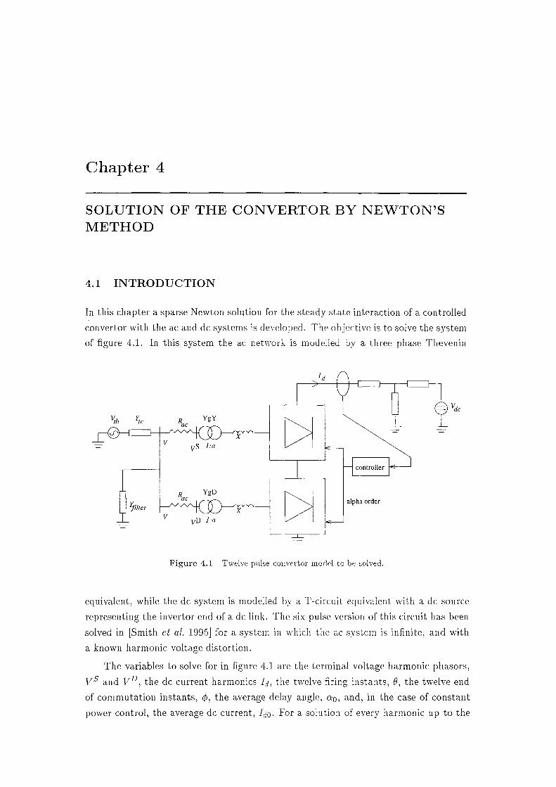
Chapter 4
SOLUTION OF THE CONVERTOR BY NEWTON'S METHOD
4.1 INTRODUCTION
In this chapter a sparse Newton solution for the steady state interaction of a controlled
convertor with the ac and de systems is developed. The objective is to solve the system
of figure 4.1. In this system the ac network is modelled by a three phase Thevenin
Vdc
v;h ~c YgY
X V vs l:a -
controller
YgD
~ 1ilter alpha order
X vD l:a
-
-
Figure 4.1 Twelve pulse convertor model to be solved.
equivalent, while t.he de s,vstcrn is modelled by a T-circuit equivalent. with a de source
representing the invert.or end of a de link. The six pulse version of this circuit has been
solved in [Smith cl al. 199:'i] for a system in which the ac system is infinite, and with
a known harmonic volt.age distortion.
'fhe variables Lo solve !'or in figure 1Ll a.re the terminal volLagE.\ harmonic phasors,
V 5 and V 1Y, the de current harmonics Id, the twelve firing instants, 0, the twelve end
of connnutation instants, ¢, the average delay angle, o:o, and, in the case of constant
power control, the average de current, Ir10. For a solution of every harmonic up to the

40 CHAPTER 4 SOLUTION OF THE CONVERTOR BY NEvVTON'S METHOD
50th, there are therefore 726 unknowns, as each harmonic requires two variables to
be specified. Being three phase and 2-port, a full specification of the terminal voltage
requires six hundred variables. If the commutating resistance, Re, is removed from
the circuit, the number of unknowns reduces to 426 since the two six pulse rectifiers
share the same ac terminal voltage. A solution for this system is developed by using
the inter-relationships of chapter 3 to write a set of simultaneous mismatch equations,
the simultaneous zero of which corresponds to the desired steady state solution. This
nonlinear problem is solved by Newton's method with sparsity, and validated against
a time domain simulation of a test system to the steady state.
4.1.1 Test System
The particular system used for the harmonic domain analysis and its time domain
validation, is the rectifier end of the model developed by the CIGRE working group 14-
02, 'Control in HVdc systems', for the purpose of comparing different controllers and
simulation techniques [Szechtman et al. 1991). The benchmark system is operationally
difficult in that it consists of a weak ac system resonant at the 2nd harmonic, coupled
via the convertor to a fundamental resonance on the de side. Although designed for
time domain and simulator studies, the benchmark is also ideal for testing the harmonic
model, as a composite ac/dc resonance at the 2nd and 1st harmonics has a larger effect
on the modulation of switching angles than other harmonics. The inverter in the
CIGRE benchmark has been removed, and modelled in the de circuit as a de voltage
source. Full parameters for the test system are given in appendix B.
4.2 MISMATCH EQUATIONS
The objective of this section is to develop mismatch equations suitable for use in New
ton's method. It is necessary first to define all the quantities that will be used by
reference to figure 4.1, to recast the relationships of chapter 3 in terms of these quan
tities, and finally to compose these relationships into a minimal set of variables and
mismatch functions. The convertor circuit of figure 4.1 will be described by the follow
ing quantities:
• V, the three phase harmonic series convertor terminal voltage.
• V}?, the voltage at the equivalent star-g/dclta tra.m,formcr prirnary, on the con
vertor side of the lumped commutation resistance. J\s shown in figure 4.1 the
transformer and thyristor conduction resistances have been lumped into an equiv
alent resistance between each bridge transformer and the ac tcrruina.l of the twelve
pulse convcrtor.
• V/i, as above f'or for the sta.r-g/star transformer.

4.2 ivIIS:MATCH EQUATIO)!S 41
• Iff, If} the phase currents flowing into the secondary windings of the star-g/star
and star-g/delta transformers, respectively.
• If,, If? the primary phase currents for the two transformers.
• Vc1k, Vc10 the de voltage harmonics and de component, respectively.
• Ic1k, Ic10 the de current harmonics and de component, respectively.
• Fao the average delay angle mismatch equation.
• Ff/, F0~, the firing angle mismatches of the thyristors in the bridges attached to
the star-g/delta and star-g/sta.r transformers, respectively.
• F£, Fi, the end of commutation mismatches in the bridges attached to the
star-g/delta and star-g/star transformers, respectively.
4.2.1 Functional Description of the Twelve Pulse Convertor
Chapter 3 developed various equations to relate quantities around the components
of a rectifier. The relationships derived are central to the convertor model, but are
quite detailed. In this chapter, those relationships are used to solve the convertor,
and it is only necessary to refer to the relationships of chapter 3 expressed in terms
of variables relevant to figure 4.1. A functional notation is therefore introduced to
describe relationships between the quantities that describe the convertor in the steady
state. The starting point will be a relationship between the convertor phase currents,
and the convertor terminal voltage.
Given the primary phase currents, the terminal voltage can be found by;
(4.1)
where the square brackets denote a three phase quantity. The AC system impedance,
[Ycc]; 1, is calculated by inverting the sum of the admittances attached to the convertor
bus. These are the filter admittance, YJilten and the Thevenin source admittance, Ytc•
This equation will be represented over all phases and harmonics by:
V = !1 (Ij,, If?) (4.2)
The convertor terminal voltage is then related to the equivalent transformer primary
voltages by the voltage drops through the equivaient commutating resistances:
[Vj]k
[vP]k
[V]k - [R3 ][IJ,]~
[V]k - [RD][If?]~.
(4.3)
( 4.4)

42 CHAPTER 4 SOLUTION OF THE CONVERTOR BY NEWTON'S METHOD
The commutating resistance matrix is assumed frequency independent and diagonal,
but possibly unba.lanced. The use of phase currents from the previous iteration in equa
tions 4.:3 and 4.4, leads to the derivation of a smaller nonlinear system in section 4.2.2.
This is denoted by the primed quantities in these equations. Using the function nota
tion again, where phase currents from the previous iteration are treated as para.meters,
not variables:
vt vf?
hW), h(V).
(4.5)
( 4.6)
Chapter :3 described how to calculate the de voltage across a six pulse bridge attached
to either a star or delta connected ac source, with inductive source impedance. Us
ing the transformer models of section :3.7, the primary voltages, Vj and VJ}, can be
transformed into equivalent star or delta connected inductive sources on the secondary
side. The de voltages across each group are then added to obtain the total de voltage,
and the constant forward voltage drop associated with each group is subtracted from
the total de side voltage direct component. The calculation of the de voltage is again
represented in functional notation:
f4(Vf, vf}, Idk, ef, ep, ¢f, <l>P),
f5(Vj, V/?, Idk, ef, ep, ¢f, ¢f).
(4.7)
(4.8)
The de voltage is functionally dependent on the switching angles since they define
the limits of the convolution analysis used to calculate the de side voltage across ea.ch
group. The de current harmonics are present in the calculation of the voltage samples
which are convolved with the sampling functions. The de voltage, when applied to the
de system, yields the de side current. For example:
summarised for any topology as:
VikYdk
(v:w - 4VJwd - Ed)Ydo•
f5(Vdk)
h(Vdo).
(4.9)
(4.10)
(4.11)
(4.12)
The de current, switching angles, and pnmary transformer voltage can be used to
calculate the transformer secondary phase currents applying the analysis of section :3.6
4.2 MISMATCH EQUATIONS
to each bridge:
43
(4.13)
(4.14)
The transformer analysis of section 3. 7 then describes how the primary currents are
obtained:
S' .f10(Js)
f11(Vj,If).
(4.15)
(4.16)
Implicit equations have been derived in chapter 3 for the convertor switching angles,
the power control, and the average delay angle. These equations, written in the form
of mismatch equations which equal zero at the solution, are summarised below and in
table 4.1.
Mj S' S' S' !12(Vp 'Idk, 0i 'c/>i) ( 4.17)
JvfD ¢, fi3(VP' Idk, 0p' ¢f) (4.18)
Mf fi4(Idk, Ida, 0f' aa) ( 4.19)
lvif fi5(Idk, Ida, 0f, aa) (4.20)
lvfs .f15(Via, Ida) (4.21)
lvfo:a fi1(Vda, Ida) (4.22)
A total of seventeen functional relationships have been described, representing 2328
equations in as many unknowns, for a solution up to the 50th harmonic. The functional
relationships are summarised in table 4.1.
4.2.2 Composition of Mismatch Functions
There is a great deal of redundancy in the system of equations summarised in table 4.1.
By a variety of substitutions of functions for variables, the number of simultaneous
equations and variables can be reduced to 426. For example, taking Ji and substituting
functions for the variables Ij, and If;:
V .fi (Ij,,I}?)
Ji (!10(Jff),f11(Vj,If))
Ji (!10(Js(Vf, Idk, Ido, Bf, ¢7)), !11 (Vf, fg(Vf, Idk, Ida, 0f, 1>f)))
!1 (!10 Us (h (V), Idk, Ido, Bf, ¢7)), !11 (h (V), fg(h (V), Idk,Ido, 0f, ¢f)))
!is (V,Idk, Ida, 0f, cpf, Bf, ¢f) ( 4.23)
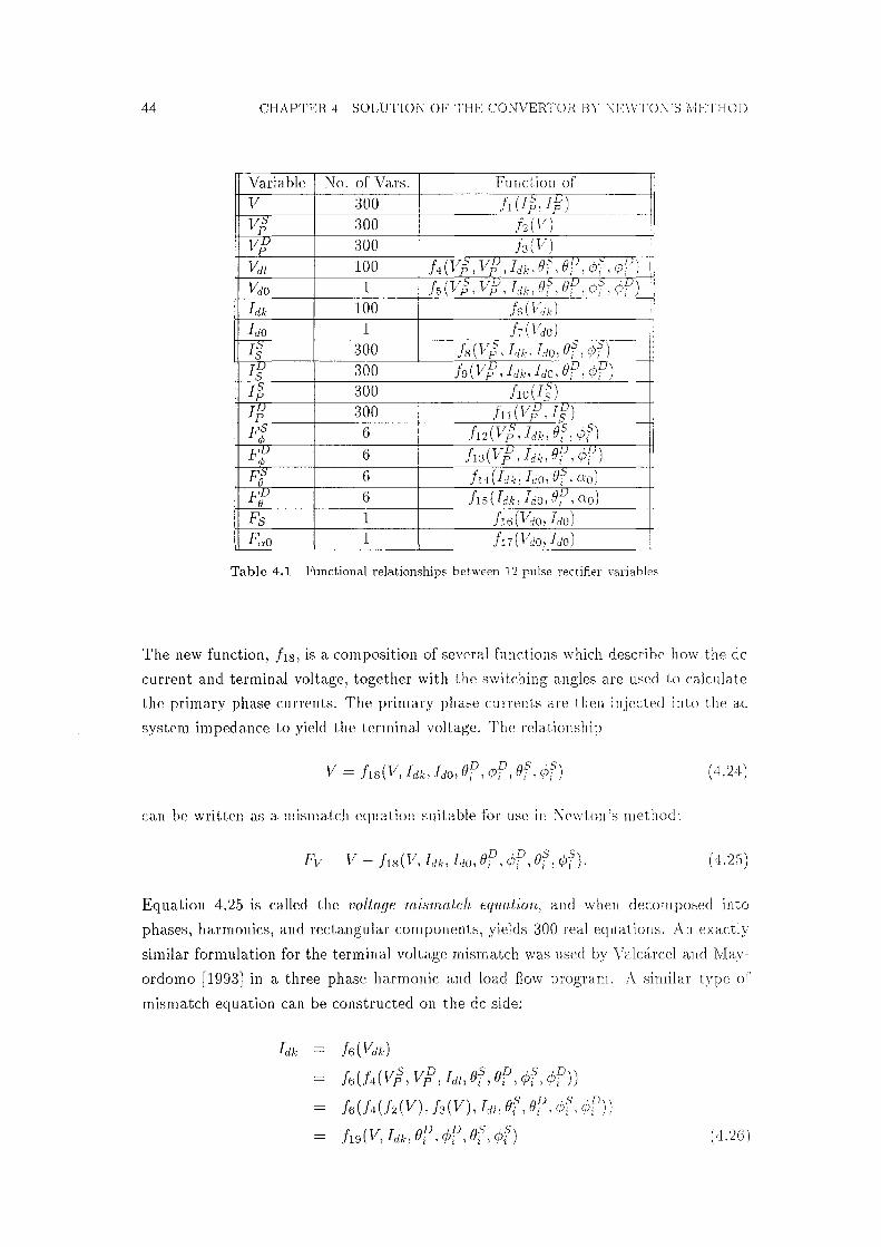
44 CHAPTER 4 SOLUTION OF THE CONVERTOR BY NEWTON'S METHOD
Variable No. of Vars. Function of V 300 Ji (I$, Ijl) V-" p 300 h(V) vlJ p 300 h(V) Vdt 100 f4(Vj; I V/J ,Idk, 0f, 01/, <P7, <j//) Vdo 1 fs(Vj;, VjJ, Idk, 0f, 01/, <Pf, <Pf) Jdk 100 /6(Vdk) ldo 1 h(Vio) J::i s 300 fs(V_ji, ldk, ldo, 0f, <Pn JlJ s 300 f9(Vf/,Jdk,ldo,0f,<Pf) p p 300 f10(Ij) JlJ p 300 fn(Vf;',If) F;t 6 f12(Vj1, ldk, 0f, ¢7)
Ff 6 f13(Vf/, ldk, 0f, <Pf) p::i
0 6 f14(Jdk, ldo, 0f, ao) Ff 6 /15 ( ldk, ldo, 0f, ao) Fs 1 fl6(Vdo, ldo) FO(o 1 f11(Vio, Ido)
Table 4.1 Functional relationships between 12 pulse rectifier variables
The new function, fi 8 , is a composition of several functions which describe how the de
current and terminal voltage, together with the switching angles are used to calculate
the primary phase currents. The primary phase currents are then injected into the ac
system impedance to yield the terminal voltage. The relationship
(4.24)
can be written as a mismatch equation suitable for use in Newton's method:
(4.25)
Equation 4.25 is called the voltage mismatch equation, and when decomposed into
phases, harmonics, and rectangular components, yields 300 real equations. An exactly
similar formulation for the terminal voltage mismatch was used by Valcarcel and May
ordomo [1993) in a three phase harmonic and load flow program. A similar type of
mismatch equation can be constructed on the de side:
ldk f6(Vik)
J6(J4(V#, vp, Id1, of, op, </Jr, </JP))
J6(f4(h(V), h(V), Id1, of, op, </Jr, </JP))
frn(V, Idk, op, </JP, of, </Jr) (4.26)

4.2 MISMATCH EQUATIONS 45
from which the following mismatch equation is constructed:
(4.27)
Equation 4.27 yields 100 equations when decomposed into harmonic real and imaginary
components, and is a composition of functions that describe the calculation of the de
voltage and its application to the de system model, to yield the de current. A further 26
mismatch equations are obtained in a similar manner, related to the convertor controller
and the switching instants:
Fj fi2(V#,ldk,0f,</>7)
fi2(h(V), Idk, of, </>7)
ho(V, Idk, of, </>7)
f13(V!J, Idk, op, <t>P)
f13(fa(V), Idk, op, <t>P)
h1 (V, Idk, op, <t>P)
Ff = fi4 (Idk, Ido, 0f, 0to)
Ff fis(Idk,Ido,0P,ao)
Fs /16(Vdo, Ida)
/16(/s(Vft, vjJ, Idk, of, op, <t>f, <t>P), Ida)
/15(/s(h(V), h(V), Idk, of, op, <t>f, <t>P), Ida)
h2(V, Idk, Ida, of, op, </>7, <t>P)
fi1(Vio, Ida)
(4.28)
( 4.29)
( 4.30)
(4.31)
(4.32)
(4.33)
(4.34)
A smaller system of 426 simultaneous mismatch equations in 426 variables has now
been developed, and is summarised in table 4.2. The reduced set of variables to be
Variable No. of Vars. Function of Fv 300 V - fis(V, Idk, Ida, 0f, </>f, 0f, </>f) Fld 100 Idk - f19(V, Idk, Ida, 0f, </>f, 0f, </>r) Fj 6 ho(V, Idk, 0f, </>?) FJ/ 6 '21 (V, Idk, 0f, </>f) p::;
0 6 /14(/dk, Ida, 0f' Oto) pu
0 6 lis(Idk, Ido, 0f, Oto) Fs 1 h2(V, Idk, Ido, 01' 0f' <l>r, <l>f) Pao 1 f23(V, Idk, Ida, 0f, 0f, </>f, </>f)
Table 4.2 Mismatches and variables for the 12 pulse rectifier.

46 CHAPTER 4 SOLUTION OF THE CONVERTOR BY NEWTON'S METHOD
solved for consists of the ac terminal voltage, the de current, the switching angles, and
the average delay angle.
It would be possible to solve for a different set of variables, however those chosen
have the advantage of being less distorted. In particular, the ac side terminal voltage
is less distorted than the phase currents, and the de side current is less distorted than
the de voltage. In fact, a fundamental frequency ac/dc load flow, will give a very
reasonable estimate of the fundamental voltage component on the ac side, and the de
current component on the de side.
The interaction of the convertor with the ac system has been specified in terms
of terminal voltage mismatch. This requires the injection of phase currents into the
ac system impedance to obtain a voltage to be compared with the estimated terminal
voltage.
The ac system interaction can also be expressed in terms of a current mismatch.
The estimated terminal voltage is applied to the ac system admittance to obtain phase
currents that are compared with phase currents calculated by the convertor model using
the estimated voltage:
Fr = [Ycc][V] - [YctHVth] - fs(h(V),Idk,Ido, ef, ¢f)
-fg(h(V),Idk,Ido,0P,¢f) (4.35)
Note that the current mismatch is still expressed in terms of the same variables as the
voltage mismatch. The current mismatch has the advantage that it doesn't require the
system admittance to be inverted, a possible difficulty if it has a high condition number.
The current mismatch is also the preferred method of modelling the interaction with a
purely inductive ac system, such as the unit connection, as the system admittance will
decrease with increasing harmonic order.
Only the voltage mismatch will be implemented here, as the ac system admittance
1s usually invertible, and the ac system impedance is typically much less than one
per unit. A hybrid mixture of voltage and current mismatches at different harmonic
orders would be the most robust and versatile approach to take; the voltage mismatch
would be used at all harmonics where the system impedance is less than one per unit,
otherwise the current mismatch would be used. In the hybrid mismatch method, the
convertor interacts with a reasonably strong ac system at all harmonic orders, and no
admittance or impedance is larger than one per unit.
The de current mismatch, Fid, defining the interaction with the de system, can
also be written as a qc voltage mismatch, Fvd, This mismatch is obtained by injecting
the estimated de current into the de system impedance and comparing the resulting

4 .. '3 NEWTON'S METHOD 47
voltage with the calculated de voltage:
(4.36)
The de voltage mismatch would be preferred in the unlikely instance of a capacitive
de system. Again, a hybrid current and voltage mismatch on the de side is the most
robust, as a series resonance can be modelled by a small impedance rather than a. large
admittance as in the de current mismatch equation. Only the current mismatch has
been implemented in this chapter, as the de side admittance to harmonics is generally
less than one per unit due to the presence of a smoothing reactor.
4.3 NEWTON'S METHOD
The mismatch equations and variables obtained in section 4.2 are a mixture of real and
complex valued. Newton's method is implemented here entirely in terms of real valued
equations and variables. All complex quantities are therefore converted into real form
by taking the real and imaginary components. A decomposition into polar components
is also possible, and this is investigated in chapter 5. A decomposition into real form is
required in any case, since the ac voltage and de current mismatch equations a.re not
differentiable in complex form. Newton's method is implemented by first assembling
the variables to be solved for into a reaJ vector X:
( 4.37)
The mismatch equations are likewise assembled into a rea.l vector:
F(X) = [R{Fv }1 .I{Fv }, R{ Fld}, I{I d}, Fe, F¢, Fao, Fidof. ( 4.38)
Given an initial estimate of the solution, .X0 , Newton's method is an iterative process
for finding the solution vector, x•, that causes the mismatch vector to be zero:
F(,r) = 0.
The iterative process is defined by;
F(XN)
_X(N+l)
pVy
XN-Y,
( 4.39)
( 4.40)
(4.41)
with convergence deemed to have occurred when some norm of the residual vector
F(XN) is less than a preset tolerance. Newton's method is not guaranteed to converge,
but convergence is likely if the starting point is close to the solution. Central to
Newton's method is a Jacobian matrix, JN, of partial derivatives. For a system of 426

48 CHAPTER 4 SOLUTION OF THE CONVERTOR BY NEWTON'S METHOD
equations, the Jacobian is 426 elements square, as it contains the partial derivative
of every mismatch function, with respect to every variable. This is illustrated for the
twelve pulse convertor functions and variables in figure 4.2, for a system with constant
current control.
There are two methods for obtaining the Jacobian elements; numerical partial
differentiation, and the evaluation of analytically derived expressions for the partial
derivatives. The numerical method is used here to validate the analytic expressions for
the Jacobian elements. Numerical calculation of the Jacobian has the advantage of ease
of coding, but is quite slow. Each column of the Jacobian requires an evaluation of all
the mismatch equations, and the resulting calculation is only an approximation to the
partial derivative. The numerical Jacobian is obtained by sequentially perturbing each
element of X, and calculating the change in all the mismatches: Jij = ;;J;; . Provided J
D..Xj is small enough, this gives a good approximation to the Jacobian.
The analytical method of calculating the Jacobian matrix requires considerable
effort to obtain all the partial derivatives in analytic form, but is exceptionally fast.
Frequently, the amount of computation required to calculate the analytic Jacobian is
of the same order as that required to calculate the complete set of mismatches just
once. For the convertor system of 426 mismatch equations, the analytic Jacobian
can be calculated in about one second, as opposed to twenty seconds for the numerical
Jacobian. The numerical Jacobian for the test system has been plotted in figure 4.3, for
a solution up to the thirteenth harmonic. This Jacobian was calculated at the solution,
and so represents a linearisation of the system of equations in table 4.2 around the
convertor operating point.
Referring to figure 4.3, the elements of the Jacobian have been ordered in blocks
corresponding to the three phases of terminal voltage, the de current, the end of commu
tation angles, the firing angles, and the average delay angle. The blocks associated with
interactions between the de current harmonics, and the ac voltage harmonics comprise
the ac/clc partition, which is 104 elements square. All other parts of the Jacobian are
called the switching terms. Within the ac/dc partition, elements have been arranged
within each block in ascending harmonic order, with the real and imaginary parts of
each harmonic a.lternati11g. Each block in the ac/dc partition is therefore 2G elements
square in figure 11.3, but 100 elements square for a solution to the fiftieth harmonic.
The .Jacobian displays several important structural features:
J\ The test system contains a parallel resonance in the ac system at the second
harmonic. This leads to rows of large terms in the Jacobian aligned with th<~
second harmonic terminal voltage mismatch (the resonance terms).
B A change in harmonic k on one side of the convertor affects harmonics k + l and
k - 1 on the other side of the convertor, causing the double diagona.l structures

"'-i'rR{ Fl a} OR{Fv:'} ar..{Fva} DR./Fva} 3R.{Fv,"} E!R.{Fv.'.'} aR { F, a\
. I· . . (- '
0 i'IR.{V~} iJI{t~;;} a~ {\/T~l} riy {l~':i} aR {1 ·,~,} c!T{Jdm} :'iD, 2 [I]
~ F1T{Fva} :3I{Fv,n} F\,a} ,"IT{F\,a} DI{F·v·n} I ;1I{F1-,a} Ft-/_' J j
k k k le ,· 0 n >rj ,:iR_{l',~':} 0_i,{t7~} aR.{l',;J i'II{V,;,} r!R {JdrrJ ;Jc,, aol 2;
Cit; :r ,- :,,-,
'"' nr..{F..1,} iJR{Fvi,} 1 :1R i·"f ('.: e-V ,,
I ,·.
"'" __ ,__l;_ .... ___ k __ 0
l'v iJR{ V,t,} f1R{V1\J ()R{ld,n) 2
• ::J if, l'\_.h} aI{Fvd fJI{Fvo} ,)I{Fv1,} ·, \ ~ r . \}J _ 8
__ __L_ __ };;_ .. - .. L. 0 E!R{V~} fJI{ Vr1~;} t~'R.{l 77~ 1 } :YR {J. 1,"
1 \ :11;_.>1 ·7 r I ,'.:;
C
aR{Fvc} Fv, I 3R.{F1,c} \ i:!R{Fv_,} ,·-rR_ { F\ ·c} I J __ },:_ k ' k ,. 0 --~ ,. :JI{-V1~} (:)y { l T7~/} ,"rR{ \ 1;;} :np·,;J r-:.)R._ { Jdm I ;~•'.,':• 1
'-< I
"' ~ J - .clT{Fvc} E!I{Fv,c} ;1I{Ft c} <1I{Fv,} ;:.,iI{Fvc} ,!T{Fvc) ;:,; __ _};;_ 0 ::; (~JR {-V7~~} cJT{t,r,~} ,"1R { \ ·,\;} ,1r{i;;U (~) rf.,1 n01 :J ~ ,...,
l!R {FJd} {'IR{F1d,} WR{F1c1,} ::rR {F1c1.} ,3R.{Flcl;.J ,3R.{ F1 d.} aR{F1c1,.} .:'IR{F1c1,} .'rR{Fu,.} 1::.1-r-;__ { F~1 ,i';_.} "' (J ::;o OR{1/7~L} aI { 1,~,:l} ah' {V,~J (jT{lr7~L} aR {1',;,} c!T {l·;,;} c!R{Tdm) DI{ f,1m} i=I!,'>, rJf1 0
s p DI{Fic1,} c!T{F1c1,.} c!T{FJdk} ,E{Frdk} c1I{F1dk} .:'II{F1c11) c!T{ Fidk} EJI{F1ai:J 1'1,,J;_-}
0 ,..., aR.{F,;;} ar {1,,~;1 } c=JR {,-,$J ,'JT{V,~l} 21}( {1"~/n} aI {11~~LT c!R {Jdm} :CJI { Ic1m) D0,
p_, (1)
i'JF,p, c_lFYi ;jp<}!I OF(:) 1 ,JF<:i1· rJF,; DI~, cJF4)1 "' ~
c!T {V~ } 0 ~
aR{iT;~} aI{l~} B'R{V,V,} (JifVrt} i'JR{v~';,) rn {jJ?{ Jdrn ) iJI { l,1m ) < (1)
?' 8F0- 8F0; 8F0- 8Fo 8Fo- 8F0; 8Fo; 8F0. 8F0; 8F0; 0 an{v~} oI{V~} 8R{VJ'i} 8I{VJ'i} 8'R{VJ,.} 8I{VJ,.} 8'R{Jdm} oI{Jdm} 80; &,:.o
81'{Fa0 } 81'{Fa0 } 8T{Fa0 } 8T{Fa0 } 8T{FO0 } 8T{Fa0 } 8T{FO0 } &I{F00 } 8I{Fc,0 } i7I{FO0 } 0 an{v~} oI{V~} o'R{VJ.} 8I{VJ,} 8R{V~} oI{Vri',} 8'R{Jdm} 8I{Jdm} 8</>; 80;
.i,.. co

,50 CHAPTER 4 SOLUTION OF THE C:ONVERTOR BY NE\:VTON'S METHOD
in the ac to de, and de to ac blocks. These are the three port terms, after [Larson
et al. 1989).
C The end of commutation mismatch is very sensitive to harmonics in the terminal
voltage and de current.
D The individual firing instants are sensitive to harmonics in the de current.
E The average delay angle mismatch, since it relates to the average de current, is
extremely sensitive to changes in the fundamental terminal voltage. There is also
some sensitivity to harmonics coupled to the fundamental; ie the 11th and 13th
harmonics on the ac side.
F As would be expected, there is strong coupling between the switching angles and
the switching mismatches.
G The Jacobian contains a strong diagonal, approximately equal to one in the ac/dc
partition. A large diagonal is often beneficial when the linear system correspond
ing to the Jacobian is solved.
There is also apparently no dependence of the terminal voltage mismatches on
the end of commutation angles, even though there is a sensitivity to the firing angles.
This seemingly anomalous result is due to the formulation of the mismatch equations.
A change in 0 moves the entire commutation current curve, whereas a change in ¢
moves only the end of commutation, consequently having a negligible effect. This
is demonstrated in figure 4.4, and it is apparent that different behaviour would be
observed with a different formulation of the mismatch equations.
The most useful feature of the Jacobian however, is the large number of small
elements. Since the Jacobian is only an estimate of the behaviour of the nonlinear
system in response to small perturbations, it is acceptable to approximate elements in
the Jacobian, without affecting the convergence of Newton's method. Small elements
may therefore be approximated by zero, making the Jacobian sparse. The sparsity
structure of the Jacobian is illustrated in figure 4.5, and again the structural elements
described above are evident. For a solution up to the fiftieth harmonic, the .Jacobian
is typically 9G% sparse. The sparsity structure of figure 1l.5 was obtained by scanning
through the Jacobian, analytically calculating selected elements, and retaining those
elements in the ac/dc partition larger than 0.05, and switching elements larger than
0.02.
In scanning the .Jacobian, it. is not necessary to calculate all elements. On the ac
or de side of the convcrtor, an odd harmonic never couples to an even harmonic, while
for transfers across the convert.or, an odd harmonic only couples to a.n even harmonic.
The total time to scan the ac/dc part.it.ion can therefore be halved by scanning with
the checkerboard pattern of figure 4.6. For a case with 50 harmonics, the bulk of

4.3 NEWTON'S METHOD
i:::: . cs:!·
:.0
... . ···P4·~·~.· . ' . . . . . . . . ' ' .. . . . . . . .. . ' ........ ~ .. . . . . . . .
. . . . . . . . . . . . . . . . . . . . . . . . . . ...... , ..... ·• ...... .
0 ..... (.) . cs:! ....... ,
0 a) C\J
. . .
CD 7 C\J O 00 CD 7 C\J
::ipi11 !uii'nvf ::n n I osqy
51
ij
I a> :S~ 0 0 "O ,-----(--
gJ u
~>
. . · ... 1~> .
1 0
Figure 4.3 Numerically calculated Jacobian for the test system: 1:1 harmonics.
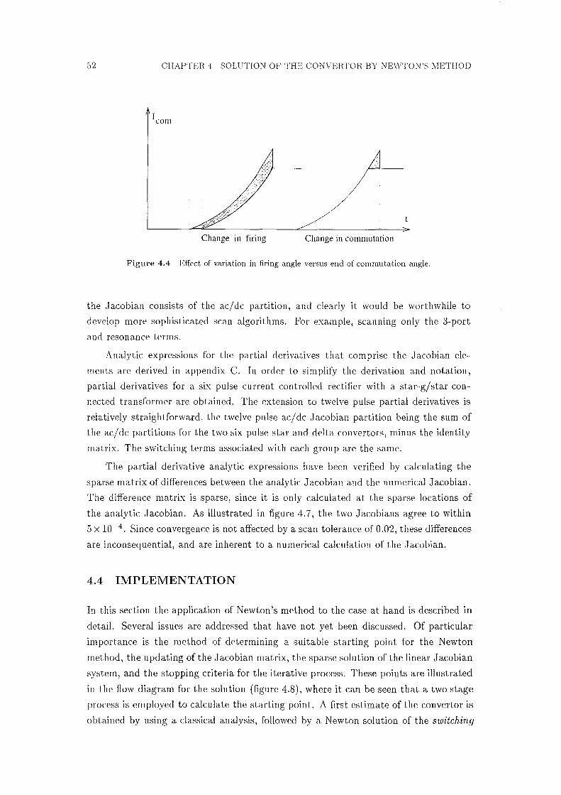
52 CHAPTER 4 SOLUTION OF THE CONVERTOR BY NEWTON'S METHOD
Change in firing Change in commutation
Figure 4.4 Effect of variation in firing angle versus end of commutation angle.
the Jacobian consists of the ac/dc partition, and clearly it would be worthwhile to
develop more sophisticated scan algorithms. For example, scanning only the 3-port
and resonance terms.
Analytic expressions for the partial derivatives that comprise the Jacobian ele
ments are derived in appendix C. In order to simplify the derivation and notation,
partial derivatives for a six pulse current controlled rectifier with a star-g/star con
nected transformer are obtained. The extension to twelve pulse partial derivatives is
relatively straightforward, the twelve pulse ac/dc Jacobian partition being the sum of
the ac/dc partitions for the two six pulse star and delta convertors, minus the identity
matrix. The switching terms associated with each group are the same.
The partial derivative analytic expressions have been verified by calculating the
sparse matrix of differences between the analytic Jacobian and the numerical Jacobian.
The difference matrix is sparse, since it is only calculated at the sparse locations of
the analytic Jacobian. As illustrated in figure 4.7, the two Jacobians agree to within
5 X 10⁻⁴ • Since convergence is not affected by a scan tolerance of 0.02, these differences
are inconsequential, and are inherent to a numerical calculation of the Jacobian.
4.4 IMPLEMENTATION
In this section the application of Newton's method to the case at hand is described in
detail. Several issues are addressed that have not yet been discussed. Of particular
importance is the method of determining a suitable starting point for the Newton
method, the updating of the Jacobian matrix, the sparse solution of the linear Jacobian
system, and the stopping criteria for the iterative process. These points are illustrated
in the flow diagram for the solution (figure 4.8), where it can be seen that a two stage
process is employed to calculate the starting point. A first estimate of the convertor is
obtained by using a classical analysis, followed by a Newton solution of the switching
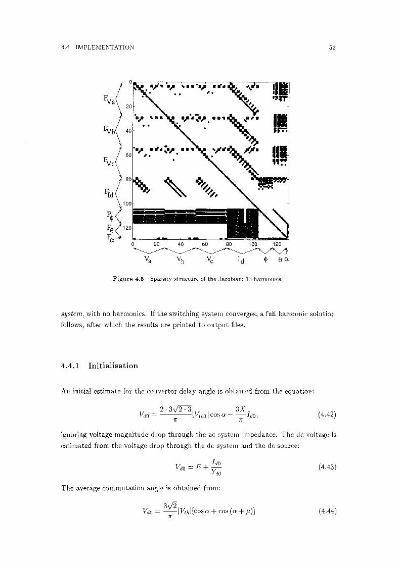
4.4 IMPLEMENTATIO~
20
40
60
FVc
80
Fld 100
Fq>
Fe 120
Fa
·.,. ..
.,. ...... ,. • rf• ,.
II H'':':
II "':!
0 20 40 60 80 100 120 ~~,,,-~
Va Vb Ve Id <j> 0 a
Figure 4.5 Sparsity structure of the Jacobian; U harmonics.
53
system, with no harmonics. If the switching system converges, a full harmonic solution
follows, after which the results are printed to output files.
4.4.1 Initialisation
An initial estimate for the convertor delay angle is obtained from the equation:
2-3~ 3X Vdo = ----IVih1I cos a - -Ido,
7r 7r ( 4.42)
ignoring voltage magnitude drop through the ac system impedance. The de voltage is
estimated from the voltage drop through the de system and the de source:
The average commutation angle is obtained from:
3J2 Vdo = -IVihl[cos a+ cos (a+ p))
7r
( 4.43)
( 4.44)

54 CHAPTER 4 SOLUTION OF THE CONVERTOR BY NEWTON'S METHOD
FVc
80
Fld 100
F<p
Fe 120
Fa 0 20 40 60 80 100 120
Va Vb Ye la <p ea
Figure 4.6 Scan structure of the sparse Jacobian; 13 harmonics.
These angles are then used to assemble the individual firing and end of commutation
angles:
/Ji+ a:
ei+µ
(4.45)
( 4.46)
These calculations yield a very rough estimate of the convertor switching angles, which
is subsequently improved substantially by a Newton solution of the switching system.
4.4.2 The Switching System
The purpose of' the switching system is to solve the relationships between the funda
mental terrnina.l voltage, the DC current, and the switching a.ngles for both bridges.
The switching syskrn is thus a complete model of the twelve pulse convertor in the
presence of' constant terminal voltage and DC current harmonics, since the harmonic
quantities appear as constant parameters. The mismatch equations and partial deriva
tives for the twelve pulse switching system ha.ve a.II been derived previously. The set of
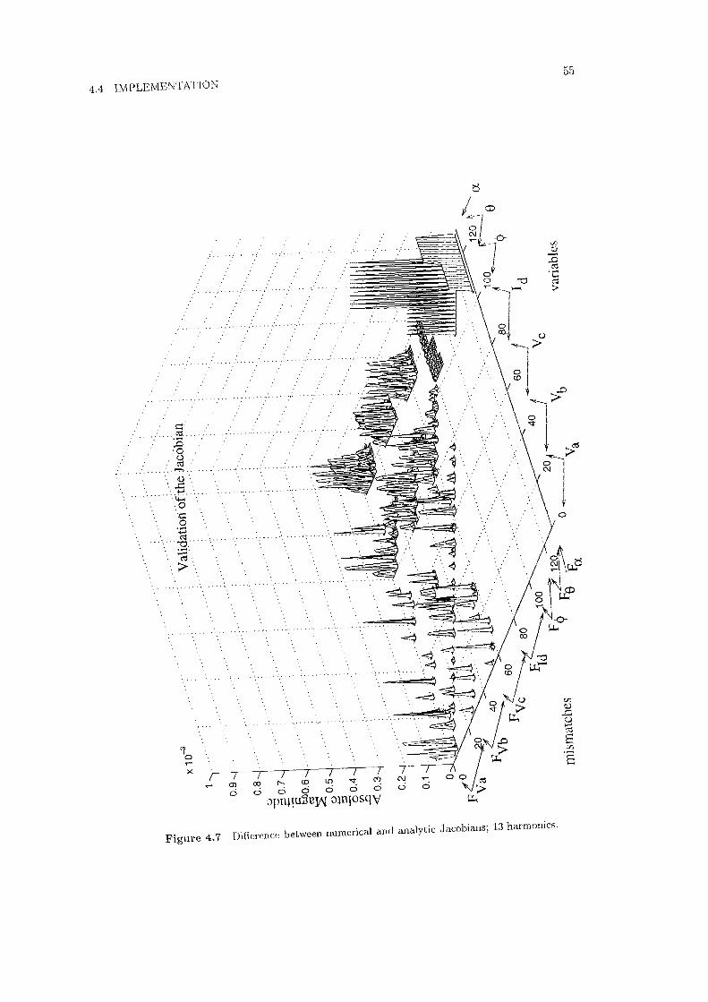
4.4 IMPLEMENTATION
. i=: .. : .. , .. c;l .... :z
0 u .:<:J
1-).
V ,s '4-,,
·o ·i= 0 .....
·. ~ ····'-.'··:st·· . -· . c-:j .
. >··.
X
.,.. ··········
···•·····--·· ...... .
'··················
······· ·-·········
.... ~. . . . . .. . . . ....
1-------r- I ..-mrot---<0~"<1:<"?
ciocidooo Jprq~u~~w gw1osqy
Figure 4.7 Difference between numerical and analytic Jacobians; 13 harmonics.
55
0
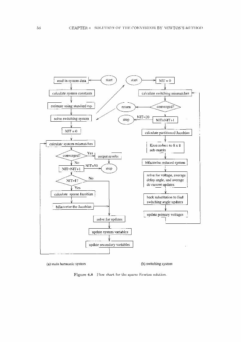
56 CHAPTER 4 SOLUTION OF THE CONVERTOR BY NEWTON'S METHOD
read in system data
calculate system constants
estimate using standard eqs
calculate system mismatches
calculate sparse Jacobian
bifactorise the Jacobian 1------;;,-i
solve for updates
update system variables
update secondary variables
NIT=O
calculate switching mismatches
NIT=20
calculate partitioned Jacobian
Kron reduce to 8 x 8 sub-matrix
bifactorise reduced system
solve for voltage, average delay angle, and average de current updates
back substitution to find switching angle updates
update primary voltages
(a) main harmonic system (b) switching system
Figure 4.8 Flow chart for the sparse Newton solution.

4.4 IMPLEMENTATION 57
equations to be solved in the switching system (for constant current control) are:
s s s . Frt,;(<Pi, oi, l1 ,Id) 0
F£ (<t>P, op, v, Id) 0
Ff (Of, lf,Id) 0
Ff (Of, Id, o:o) 0
Fv1 ( <t>f, of, V,Id) 0
Fa0 ( <l>f, Of, V, Id) 0. (4.47)
A flow diagram for the switching system is shown in figure 4.8, part (b), while
the structure of the switching Jacobian can be seen in figure 4.9. Those elements
corresponding to the partial derivatives of voltage mismatch with respect to end of
commutation angle have been set equal to zero, since they are always insignificant.
9 8
0 . • • • . . . .
5 • • . • • •
• . . 10 •
• A
• •
• • .
• •
25 • • • . . . . • . • • . . . • • C ' • • • • . •
' • • • • • • • • • • • • • • 30 . • • • • • . .
• • • • • • • • • • • • • • • • • • • • • • • • • • • • • • • • • • • • • • • •
0 5 10 15 20 Variable number
• • • • • . • • • . • • • • . .
• . . • • •
• • • • • .
• •
• •
• • • • . . • • . • • • • • • • • . • . • • • • • • • • • • • • • • • • • • • • • • • • • • • •
25
• • • • • • • . • . • . • • . . • • • • • • • • • . • • . • • • . . • • • • • • • . . . B~
• • • • . . . • D . .
• • • • . . • • • • • • • • • •
30
• . • • • • • • • . • •
• • • • • • • • • • . •
• • • • • . • •
8
"'o I dO
Figure 4.9 Sparsity structure of the switching Jacobian matrix (power control).
This Jacobian is quite sparse, and always has the same sparsity structure, however
it is of an intermediate size, being too small for a general purpose sparse solution, and
yet large enough to be significant. In the case of an inter harmonic model, the switching
Jacobian would be of size 24n+8, where n is the number of cycles over which the steady
state is defined. It is therefore worthwhile to develop an 'ad hoc' sparse solution of the

58 CHAPTER 4 SOLUTION OF THE CONVERTOR BY NEWTON'S METHOD
switching Jacobian, and the best way to do this is to employ a partitioning method.
With reference to figure 4.9, the partitioning method exploits the fact that the
top left hand part of the switching Jacobian, A, is almost diagonal, and can easily be
reduced to the identity matrix. It is then straightforward to create a reduced system
of size 8 x 8 by multiplying the rectangular cross coupling partitions, C and B, to
give D - CB. In this case the cross coupling matrix multiplication is very fast, since
the variables have been ordered so that most of the nonzero elements of each of the
cross coupling partitions correspond to the zeros of the other. Using this method,
the linear system can be solved in approximately 1000 flops, instead of some 10 000.
Indexing overheads have been virtually eliminated by storing partial derivatives directly
into specific vectors, and then using 'ad hoc' code for the partitioning method. The
reduced 8 X 8 system is solved by LU decomposition for the terminal voltage, average
delay angle, and de current order updates. These are then backsubstituted to find the
switching angle updates.
The switching Jacobian is updated every iteration of the Newton method, and
convergence has been found to be rapid and robust. The convergence criteria for the
switching system is:
IFVil < 0.001 IVil IFr1I < 0.001 IIil
IFaol < 0.001 !Idol
IFidol < 0.001 IPI !Feil < 5 X 10⁻⁸
IF¢; I < 5x10⁻⁸ . ( 4.48)
Convergence typically occurs in 4 to 10 iterations, for starting terminal voltages ranging
from 0.3 to 7 p.u. A case with a system impedance of 1.3 p.u. at the fundamental has
been solved (which required 11 iterations). A failure to converge in 20 iterations has
so far always implied that the system has no solution. An invalid solution (eq negative
firing angle) has never occurred, nor have multiple valid solutions been observed. If the
de voltage source is negative, the system will solve as for a current controlled inverter.
The solution obtained with the switching system is an excellent starting point for
the full harmonic solution, as the switching angles are largely determined by interactions
at the fundamental frequency. Since the switching system is three phase, it includes
the effect of any unbalance. The switching system is utilised in chapter 5 as part of a
fast decoupled convertor solution, and has also been interfaced to a three phase load
flow.
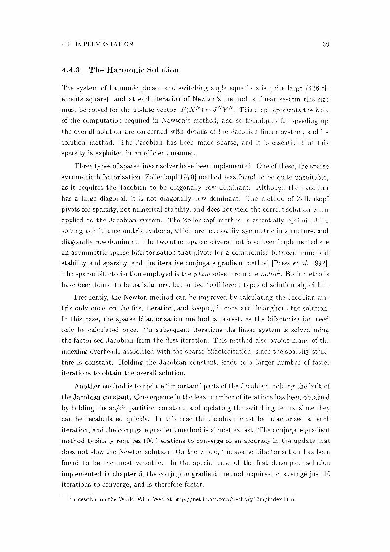
4.4 IMPLEMENTATION 59
4.4.3 The Harmonic Solution
The system of harmonic phasor and switching angle equations is quite large ( 426 el
ements square), and at each iteration of Newton's method, a linear system this size
must be solved for the update vector: F(XN) = pVyN_ This step represents the bulk
of the computation required in Newton's method, and so techniques for speeding up
the overall solution are concerned with details of the Jacobian linear system, and its
solution method. The .Jacobian has been made sparse, and it is essential that this
sparsity is exploited in an efficient manner.
Three types of sparse linear solver have been implemented. One of these, the sparse
symmetric bifactorisation [Zollenkopf 1970] method was found to be quite unsuitable,
as it requires the .Jacobian to be diagonally row dominant. Although the Jacobian
has a large diagonal, it is not diagonally row dominant. The method of Zollenkopf
pivots for sparsity, not numerical stability, and does not yield the correct solution when
applied to the Jacobian system. The Zollenkopf method is essentially optimised for
solving admittance matrix systems, which are necessarily symmetric in structure, and
diagonally row dominant. The two other sparse solvers that have been implemented are
an asymmetric sparse bifactorisation that pivots for a compromise between numerical
stability and sparsity, and the iterative conjugate gradient method [Press et al. 1992].
The sparse bifactorisation employed is the y12m solver from the netlib1• Both methods
have been found to be satisfactory, but suited to different types of solution algorithm.
Frequently, the Newton method can be improved by calculating the Jacobian ma
trix only once, on the first iteration, and keeping it constant throughout the solution.
In this case, the sparse bifactorisation method is fastest, as the bifactorisation need
only be calculated once. On subsequent iterations the linear system is solved using
the factorised Jacobian from the first iteration. This method also avoids many of the
indexing overheads associated with the sparse bifactorisation, since the sparsity struc
ture is constant. Holding the Jacobian constant, leads to a larger number of faster
iterations to obtain the overall solution.
Another method is to update 'important' parts of the Jacobian, holding the bulk of
the Jacobian constant. Convergence in the least number of iterations has been obtained
by holding the ac/dc partition constant, and updating the switching terms, since they
can be recalculated quickly. In this case the Jacobian must be refactorised at each
iteration, and the conjugate gradient method is almost as fast. The conjugate gradient
method typically requires 100 iterations to converge to an accuracy in the update that
does not slow the Newton solution. On the whole, the sparse bifactorisation has been
found to be the most versatile. In the special case of the fast decoupled solution
implemented in chapter 5, the conjugate gradient method requires on average just 10
iterations to converge, and is therefore faster.
1 accessible on the World Wide Web at http://netlib.att.com/netlib/y12m/index.html

60 CHAPTER 4 SOLUTION OF THE CONVERTOR BY NEWTON'S METHOD
There are better iterative methods than the conjugate gradient, such as the precon
ditioned biconjugate gradient, that have not been implemented. The preconditioned
biconjugate gradient method can be used efficiently if a sparse approximation to the
inverse of the Jacobian can be created. This is very likely, as the inverse of the Jacobian
contains many small elements. A final advantage of the conjugate gradient methods is
that they can be easily implemented on a parallel processor, as the algorithm is based
on successive sparse multiplications of the .Jacobian by a vector.
4.4.4 Convergence Tolerance
The basic requirement of convergence is that all of the mismatches F(X)i are small
enough. The mismatches however, are of several types, entailing a different convergence
requirement for each type of mismatch. The convergence tolerances are listed below:
IFVkl < 0.001
!Vkl IFnl
< 0.001 lhl !Fldl < 0.001 II di
IFaol < 0.001 !Idol
IFidol < 0.001
!Pl IF0;I < ,5 X 10-8
IF¢;! < 5 X 10⁻⁸ . (4.49)
Note that convergence tolerance for the complex mismatches, Fv, Fr, Fld is expressed
in terms of the magnitude of the mismatch. This means that the error in an estimated
value for a variable , for example Vii, is smaller than 0.1% of its own length. The
advantage of a relative mismatch of this type, is that it treats all harmonics equally.
However to prevent an attempt to converge to an absolute error of zero for harmonics
that arc not present (eg even harmonics in some cases), this convergence test is only
applied to harmonics that have a size larger than rn- 5 per unit. These convergence
tolerances can be made tighter to obtain more accurate solutions if necessary. A relative
convergence tolerance of 2 x 10⁻⁶ has been used in the impedance calculations of
chapter G.
The tolerance set for the switching mismatches of 5 x l o-8 corresponds to 1 .t1 x 1 o-,t degrees at the 50th harmonic, or 0.1 nsec. This high tolerance has been used in the
calculation of' the convertor impedance, and docs not require any extra iterations.
Another type of co11vcrgc11ce tolerance that can be used, is to calculate a norm of the

4.5 VALIDATION AND PERFORMANCE 61
real mismatch vector; for example, the 1-norm:
n
IXl1 = I:!Xd (4.50) i=l
A tolerance of IXl 1 < 10-5 is suitable for general purpose use. This type of convergence
test is fast and easy to apply, but does not imply that all harmonics have converged to
a satisfactory accuracy.
4.5 VALIDATION AND PERFORMANCE
The model was verified against time domain simulation of the test system described
in appendix B, using the program PSCAD/EMTDC. The steady state solution was
obtained by simulating for one second, with a time step of 20µs, and then obtaining
waveforms over one cycle for subsequent comparison with the harmonic domain solu
tion. The results of four tests are given here, comparing the de voltage and ac phase
current waveforms and spectra, since these quantities are the most distorted. The tests
are designed to highlight any modelling, and convergence deficiencies. The tests carried
out were:
Test 1: A base case solution with no harmonic sources in the ac system.
Test 2: The Thevenin voltage source in the ac system was distorted by 5% positive se
quence second harmonic. This excites the composite ac/dc system resonance,
leading to noncharacteristic harmonics, and a high degree of interaction between
convertor switching angles and the ac/dc harmonics.
Test 3: The leakage reactance of the phase 'b' star-g/delta transformer was increased from
0.18 to 0.3 per unit. This imbalance causes the generation of odd harmonics, and
a relatively large coupling to the zero sequence, which is illustrated in figure 4.14.
Test 4: A 0.1 per unit resistance was placed in series with the star-g/delta transformer,
and the secondary tap changer of that transformer was set to 1.1 p.u. Convergence
with such a large series resistance indicates that the effect on convergence of not
representing commutation resistance in the Jacobian is acceptable. Setting the
tap changer on one transformer but not the other introduces six pulse unbalance.
It was necessary to increase the ac system fundamental source from 1.10976 to
1.20976 p.u. to enable the current order to be satisfied.
The results of test one, the base case, are shown in figures 4.10 and 4.11. It can
be seen from the spectra that only the characteristic harmonics are present, and that
there is a close match between the time and harmonic domain solutions. The time
domain solution yielded small residual non-characteristic harmonics in the spectra,

62 CHAPTER 4 SOLUTION OF THE CONVERTOR BY NEWTON'S METHOD
which were suppressed in the phase graphs. The de voltage waveform was generated
from the harmonic domain solution by plotting the Fourier series for each de voltage
sample during the appropriate interval, rather than inverse transforming the de voltage
spectra. This eliminates Gibbs phenomena associated with the step changes in voltage,
but gives overly sharp voltage spikes. These are not present in the time domain solution
clue to modelling of the snubber circuits, which limit the dd~. The time domain derived
de voltage waveform is therefore more rounded. Clearly, if an accurate time domain
waveform was required from the harmonic domain solution, it would be necessary
to post process the waveshape using knowledge of the snubber circuit time domain
response. The comparison of the waveshapes indicates that all the switching angles are
correct.
i,iVhen a second order harmonic voltage source was placed in the ac system, the
composite resonance was excited, resulting in non-characteristic harmonics. Referring
to figures 4.12 and 4.13, odd harmonics are present on the de side, and even harmonics
on the ac side. In particular, the fundamental resonance on the de side is excited, and
there is a large fundamental component in the de voltage.
Unbalancing the star-g/delta transformer leakage reactance (figures 4.14 and 4.15),
caused the generation of many harmonics, and a large zero sequence on the ac primary
side. This is clue to sequence transformation by the transformer, irrespective of its
connection to a. convertor. The zero sequence has been plotted in figure 4.14, and the
close agreement with the time domain solution is evident. The final set of results,
figures 4.16 and 4.17, shows the expected generation of six pulse harmonics due to
imbalance between the two six pulse groups.

4.5 VALIDATION AND PERFORMANCE
DC voltage, Test One 0.5.---mrr----.-------.------,---------,,-------,----,-------.------,-,
Q) en
0.4
0.3 ...
0.2
0.1'"
100
~ -100
0...
0.14 ,-.._
d 0.12
r:i. "-' 0.1
~ 0.08
--~ 0.06
@) 0.04 ro 8 0.02
EMTDC Harmonic Domain ~~
harmonic order
DC voltage, Test One
harmonic order
Phase A current, Test One
EMTDC Harmonic Domain
~~
-
-
-
o~~--~--~-~~--~-~~-~~--------~-~~ 40
,-.._ v:, Q) Q) 100 I-< bi} Q)
0 5 10 15 20 25 30 35
harmonic order
Phase A current, Test One
"d 0._...."--m-------~~~-------,.._~-------,.._~--"-'
Q) v:,
~ -100
0...
0 5 10 15 20 25 30 35 40
63
Figure 4.10 Comparison of time and harmonic domain solutions for phase currents and de voltage spectra: Base Case
64 CHAPTER 4 SOLUTION OF THE CONVERTOR BY NEWTON'S lVIETHOD
Phase currents, Test One
2
-2
-3'-----''---------'--~---'-------'---__,_---'------'----'-----~
0
,--,, 550 ~ '-'
<1) 01)
~500 0 >
450
0.002 0.004 0.006 0.008 0.01 0.012 0.014 0.016 0.018 0.02
time (sec)
DC voltage, Test One
400'-------'-----'------.l..-------'-----'----'-----'-------'----'-----' 0 0.002 0.004 0.006 0.008 0.01 0.012 0.014 0.016 0.018 0.02
time (sec)
Figure 4.11 Comparison of time and harmonic domain solutions for phase current and de voltage waveforms: Base Case.

4.5 VALIDATION AND PERFORMANCE
Phase cunents, Test Two
2
-2
_3L-----"'----------'------'-----'----'-------'------'-------'----'----~
0
,......,550
~ '-"' <I) bJ)
.§ 500 0 >
450
0.002 0.004 0.006 0.008 0.01 0.012 0.014 0.016 0.018 0.02
time (sec)
DC voltage, Test Two
400~-~-~--~-~-~--~-~-~--~-~ 0 0.002 0.004 0.006 0.008 0.01 0.012 0.014 0.016 0.018 0.02
time (sec)
65
Figure 4.12 Comparison of time and harmonic domain solutions for phase current and de voltage waveforms: Test 2.

66 CHAPTER 4 SOLUTION OF THE CONVERTOR BY NEWTON'S METHOD
DC voltage, Test Two ,,-__ 0.5 ,.....,.-,,--------,-------.-----,-----,,-----,------.-----.------.--,
::i 0.. 0.4 '-" Q)
'"C) 0.3
.a ...... i::: 0.2 bl) (rj
S 0.1
Q) Cl)
100
~ -100
0..
0.14 ,,___ ::i 0.12
0.. '-" 0.1
~ 0.08
. .§ 0.06
5h 0.04
S 0.02
0
0 0
,,___ Cl) Q) Q) 100 I-< bl) Q)
EMTDC Harmonic Domain
5
~ ~
10 15 20 25
harmonic order
DC voltage, Test Two
harmonic order
Phase A current, Test Two
EMTDC Harmonic Domain
~~
5 10 15 20 25
harmonic order
Phase A current, Test Two
30 35 40
30 35 40
~ o,_,_.-'-.-,,-~-----~~~~~---~ ....... ..-.~~~----~~---
Q) Cl)
crj -100 ..c1 0..
0 5 10 15 20 25 30 35 40
Figure 4.13 Comparison of time and harmonic domain solutions for phase currents and de voltage spectra: Test 2.

4.5 VALIDATION AND PERFORMANCE 67
,.-._
~ '--' ..... c:: ~ ::l u
,.-._
~ '--'
Q.)
~ ..... 0 >
,.-._
~ '--' .....
c:: Q.)
t:: ::l u
3
2
1
0
-1
-2
-3 0
550
500
450
Phase currents, Test Three
0.002 0,004 0.006 0.008 0.01 0.012 0.014 0.016 0.018 0,02 time (sec)
DC voltage, Test Three
400'--~--~--~--~--~--'--~-----~-~ 0 0.002 0.004 0.006 0.008 0.01 0.012 0.014 0.016 0.018 0.02
time (sec)
Zero sequence ac current, Test Three
0.1
0
-0.1
-o.2~-~-----~--~--~-~--~--~-----0 0.002 0.004 0.006 0.008 0.01 0.012 0.014 0.016 0.018 0.02
time (sec)
Figure 4.14 Comparison of time and harmonic domain solutions for phase current and de voltage waveforms: Test 3.

68 CHAPTER 4 SOLUTION OF THE CONVERTOR BY NEWTON'S :METHOD
DC voltage, Test Three ,,.--__ 0.5 ~~--~---~---~---~------.---~---~-----.---,
~ 0.. 0.4
'--' (l)
"O 0.3
3 ..... i:;::: 0.2 on crj
8 0.1
(l) Cll
100
~ -100
0..
0.14 ,,.....__
d 0.12
0.. '--' 0.1
~ 0.08
.-s o.oa ~ 0.04 crj
8 0.02
0
EMTDC Harmonic Domain
5
~~
10 15 20 25
harmonic order
DC voltage, Test Three
harmonic order
Phase A current, Test Three
EMTDC Harmonic Domain
~~
30 35 40
0 L--1.-11.JL--"-'--_..JW'--LLL.---'-Ll-'-"-'---11.J'--"'-'--11.J'--....... --'-'"'--'-'-'-----'W'--'-'-'---LIJL-L-'-'-'----""'--....__u_.___=-..,.__,
40
(l) Cll
100
~ -100
0..
0
0
5 10
5 10
15 20 25 30 35
harmonic order
Phase A current, Test Three
15 20 25 30 35 40
Figure 4.15 Comparison of time and harmonic domain solutions for phase currents and de voltage spectra: Test 3.

4.5 VALIDATION AND PERFORMAKCE
2
~ 0 ;:; (.)
-1
-2
Phase currents, Test Four
_3L...----'---'----'----'----'-----'-------'-----'----'----~ 0
~550 > ~ '_,/
(1.) bi)
.§ 500 0 >
450
0.002 0.004 0.006 0.008 0.01 0.012 0.014 0.016 0.018 0.02
time (sec)
DC voltage, Test Four
400~-~-~--~-~-~--~-~-~--~-~ 0 0.002 0.004 0.006 0.008 0.01 0.012 0.014 0.016 0.018 0.02
time (sec)
69
Figure 4.16 Comparison of time and harmonic domain solutions for phase current and de voltage waveforms: Test 4.

70 CHAPTER 4 SOLUTION OF THE CONVERTOR BY NEWTON'S METHOD
DC voltage, Test Four ,,-.__ 0.5 ~~--~---~---~--~~--~---~---~---~
.:! 0.. 0.4 .___, Q)
"Cl 0.3
.a ..... f::: 0.2 bl} C'd S 0.1
Q) ell
100
.a -100
0..
0.14 ---::i 0.12
0.. .___, 0.1
~ 0.08
. .§! 0.06
Sn 0.04 C'd S 0.02
Q) ell
0 0
100
.a -100
0..
EMTDC Harmonic Domain ~~
EMTDC
~
5 10
harmonic order
DC voltage, Test Four
harmonic order
Phase A current, Test Four
Harmonic Domain
15 20 25
harmonic order
Phase A current, Test Four
30 35 40
Figure 4.17 Comparison of time and harmonic domain solutions for phase currents and de voltage
spectra: Test 4.

4.5 VALIDATION AND PERFORMANCE 71
Convergence of the sparse Newton solution is fast and robust, even if the Jacobian
matrix is held constant. A convenient measure of the convergence is the 1-norm, the
sum of the magnitudes of all the mismatches. At each iteration the 1-norm is reduced
by an approximately constant convergence factor, >., depending upon the difficulty
of the system, and whether the switching terms are updated. The constant conver
gence factor is evident in figures 4.18 and 4.19, which show the decreasing 1-norm as
a function of iteration number for all five test cases. Note that the final 1-norm at
convergence varies according to the test, as the required convergence of a particular
small noncharacteristic harmonic may require more iterations. An additional test has
also been plotted, test five, where a 20% second order harmonic source was placed
in the ac system. As indicated in table 4.3, a smaller convergence factor ( and hence
fewer iterations to convergence) is obtained if the switching terms are updated (rows
with subscript 'a'). However the constant Jacobian method is always faster as each
iteration takes approximately 0.6 seconds as opposed to 2.3 seconds. The constant
Jacobian method is only slower if it requires more than four times as many iterations
to converge. The only situation in which this has been observed is when the composite
resonance is excited by a very large (0.3 p.u.) second harmonic source. The constant
Jacobian method is therefore likely to be faster in any realistic case.
Test No. CPU time Switch Main >. (seconds) Iterations Iterations
la 15.5 6 4 0.1314 lb 11.1 6 6 0.1712 2a 24.9 6 8 0.1440 2b 14.8 6 11 0.2562 3a 17.7 6 5 0.1069 3b 12.3 6 7 0.1130 4a 22.7 9 7 0.2498 4b 14.1 9 9 0.3129 5a 31.5 6 11 0.3068 5b 20.8 6 21 0.5382
Table 4.3 Convergence and performance of the solution a) updating switching terms, b) constant Jacobian.
It is evident from table 4.3 that convergence is slowed by the low ·harmonic order
composite resonance, and by the presence of a large commutating resistance. The
second order harmonic composite resonant is particularly difficult for the constant
Jacobian method, as there is a higher coupling between low order harmonics and the
switching angles. This is evident in the convergence of Test 5, which required 21
iterations. For more realistic systems, convergence in eight iterations using a constant
Jacobian might be expected. The execution times listed in table 4.3 are for a Sun
Sparcstation IPX.

72 CHAPTER 4 SOLUTION OF THE CONVERTOR BY NEWTON'S 1\iIETHOD
Convergence with updated Switching Terms 10' ,---,-------,----.----.--.----,------r---.-----r-------.
10-•,_____,_ _ _._ _ _,___--'----'-----'----'-~-'----'-----' 1 2 3 5 6 7
lterallon number 8 9 10 11
Figure 4.18 Convergence with the switching terms updated each iteration.
Convergence with constant Jacobian 10• ~-------,---.------.---~--~
5 10 15 20 25 llerallon number
Figure 4.19 Convergence with the Jacobian held constant.
4.6 NEW ZEALAND SOUTH ISLAND SYSTEM
The results of the previous section show that the harmonic convertor model yields
essentially the same solution as an EMTP based simulation to the steady state. One of
the main advantages of harmonic domain analysis is that the frequency dependence of
the ac system impedance can be calculated with relative ease. It is therefore possible
to use the harmonic convertor model to calculate the interaction with any ac system
for which a harmonic penetration is available. For this next study, the ac system of
the CIGRE benchmark was replaced by the three phase harmonic impedance of the

4.6 NEW ZEALAND SOUTH ISLAND SYSTE:rvl 73
New Zealand South Island system, looking from the Benmore 220kV bus (since there
is a HVdc link convertor station there). The use of per unit quantities in the convertor
model allows a direct connection, despite the difference in voltage levels. The hybrid
CIGRE/NZ test system is described in appendix B
Since the New Zealand South Island system is stronger than the CIGRE system,
and lacks difficult composite resonances, solution of the unified method was rapid,
converging in 7 iterations to a 1-norm residual of 6 X 10⁻⁶p.u. The system impedance
used at each harmonic was a full 3 X 3 matrix, and so the effect of intersequence
coupling and impedance unbalance was modelled in this solution. To determine the
nature of this effect, the off diagonal impedance matrix terms were set to zero to remove
intersequence coupling, and the remaining diagonal terms were made equal (balanced).
The solution obtained with a balanced impedance is representative of what may be
expected from a single phase harmonic model. The terminal voltage and phase current
harmonics are compared in figure 4.20.
phase A current (magnitude) 0.08 ~-.--------,-----,----,-------,-----.-----.---------,-----,
-s-0.06 -9: -C: ~ 0.04 ... ::, (.)
(.)
ro 0.02
Left - three phase
Right - balanced
0L.......Ll-'---Ll....----'------L'-'-....,_____....'--=------'-----C.----'-'-'--........ -.<1.-_ _.___ __ ___.._.___~~,_,
0 5 1 0 15 20 25 30 35 40 Harmonic
phase A voltage (magnitude)
Left - three phase
Right - balanced
0'-'-'-'-----'-'-----'-----'-'-'-....,__~-~----'-~~~~-~-~-~~~~-~
0 5 10 15 20 25 30 35 40 Harmonic
Figure 4.20 Comparison of solutions for the South Island system with full and balanced ac system impedance.
The effect of unbalance m the ac system impedance 1s to promote the injection of
74 CHAPTER 4 SOLUTION OF THE CONVERTOR BY NEWTON'S METHOD
triplen harmonics by the convertor. The triplens are primarily positive and negative
sequence, and of a substantial magnitude.
4.7 CONCLUSION
L' sing the interelationshi ps of chapter 3 a functional description, of the twelve pulse con
trolled rectifier, with ac and de system representation, has been made. This functional
description has been used to assemble a reduced set of mismatch equations suitable for
use in Newton's method. The Newton's method solution was then described, and the
Jacobian matrix of partial derivatives used in this method analysed. The Jacobian ma
trix displays several structural features, such as resonance terms and three port terms
that are related to the interaction of the convertor with the ac and de systems. The
Jacobian matrix can be made sparse by setting small elements to zero.
The implementation of Newton's method for the case at hand has been described,
with particular attention given to the starting point for the Newton procedure, and the
convergence criteria. A Newton solution at the fundamental frequency, has been shown
to provide a good estimate of the switching angles even with an unbalanced and weak
ac system. Two methods of solving the sparse Jacobian system were described, with
a direct sparse bifactorisation method preferred at present, given that the Jacobian is
held constant.
The convertor model was verified against time domain solutions using the program
PSCAD/EMTDC, for the rectifier end of the CIGRE benchmark model. Excellent
agreement was obtained between the two solutions even in the presence of unbalance
in the convertor transformer, and excitation of a composite ac/dc system resonance.
Convergence was· rapid, although slowed slightly by a large commutating resistance.
Despite requiring more iterations, fastest convergence was obtained when the Jacobian
was held constant.
Interaction of the CIGRE benchmark rectifier with the New Zealand South Is
land system was solved by using a suite of harmonic penetration software to calculate
the South Island system equivalent impedance at the BENMORE-220 bus. The so
lution was obtained rapidly, and predicted the generation of noncharacteristic triplen
harmonics by the rectifier due to unbalance in the ac system impedance.
Neither invalid, nor multiple solutions have been observed with the convertor model
to date. However in general, multiple solutions must exist, and an example of an
unstable periodic solution for a nonlinear system is given by Aprille and Trick [1972].
There is therefore some incentive to develop a postprocessing stage to check the validity
of the solution. To date, the model has simply diverged if no solution is possible (for
example the current order is too large for the strength of the ac system).
The model described here can be made more robust with respect to commutating

4.7 CONCLUSIO;,' 75
resistance by using 726 mismatch equations instead of 426, as this allows a full repre
sentation of the commutating resistance in the Jacobian. In this case both ac system
terminals would be represented, and the solution would be for VD and V 5 . This ap
proach would allow the modelling of skin effect in the transformers, and its effect on
the convertor impedance for example, although would be slightly slower for systems
with little commutating resistance. It is suggested that a hybrid voltage and current
mismatch implementation would also better handle large impedances in the ac system.
The description of the system in terms of functions affords a modular implemen
tation of the model. For example, the functions that describe transfer through the
convertor transformer could readily be extended to cover other transformer connec
tions. The Jacobian matrix itself retains the same structure, even in multicon vertor
systems or when interfaced to a load flow. In either case, the Jacobian matrix described
here would be a block in a block diagonal system Jacobian with linear coupling terms
to other nonlinearities.
Other methods of improving the convertor model are possible, such as a polar coor
dinates•implementation, a fast decoupled solution, or a sequence components solution.
These possibilities are investigated in the next chapter, where only the latter is found
to be worthwhile.

Chapter 5
ALTERNATIVE IMPLEMENTATIONS
In this chapter three alternative implementations of the convertor model are investi
gated, with a view to obtaining faster, or more robust solutions. Existing practice with
the load flow problem suggests two possible modifications to the convertor model; a
polar components specification of the mismatch equations and variables, and a fast de
coupled solution method. With the polar components method it is hoped to find little
coupling between mismatch angles and variable magnitudes and vice versa. This would
enable the implementation of a decoupled solution, where two decoupled Jacobians are
used to update magnitudes and phase angles separately. Even without the polar com
ponents representation of ac/dc harmonics, a decoupled solution is still possible, and is
implemented below by decoupling the convertor switch system variables and the ac/dc
side harmonics.
Any alternative to a rectangular phase components model is achieved by an appro
priate transformation of the existing variables and mismatch equations. This means
that the analyses of chapters 3 and 4, and the derivation of the Jacobian in appendix C
are all still useful. An example is the sequence components transformed model, derived
in section 5.3, where the Newton solution algorithm can be written in terms of the ex
isting phase components solution using a matrix, T, based on the sequence transform
matrix:
UN TXN
VN T F(XN)
VN T Jr- 1 zN
u(N+i) uN-zN
x(N+l) r-1u(N+1) (5.1)
The quantity T JT- 1 is the transformed Jacobian, obtained in this case by means of
linear transformation. The transformation to polar coordinates is not linear, however
a very similar approach, using the chain rule, is described below.
78 CHAPTER 5 ALTERNATIVE IMPLEMENTATIONS
5.1 POLAR TRANSFORMS
The motivation for developing a polar transformed solution is the expectation that a
change in the magnitude of a harmonic will affect mainly the magnitude of harmonics
coupled to it, and similarly for the phase. It is thus hoped to make the ac/dc partition
more sparse by eliminating coupling between phase angles and magnitudes. A polar
transform has the additional advantage of being simple to implement and calculate.
In order to simplify the notation, the polar method is described with reference to a
'generic' non-analytic complex function G, which is a function of the complex variable
x. The following notation is also useful in referring to their rectangular or polar parts:
GR real part of G
Gr imaginary part of G
Gu magnitude of G
Ge angle of G
XR real part of x
Xr imaginary part of x
X1vf magnitude of x
Xg angle of x
The quantities GR, Gr, XR, xr are assumed known, as are the partial derivatives ~~~, oGa oGr d oGr G d G d"l d ,· d· ox
1 , oxR, an ox
1. 1w an 0 are rea 1 y enve .
and
G Gr
0 = arctan GR
(5.2)
(5.3)
GR and Gr can be considered to be functions of the real and imaginary parts of x,
which in turn are functions of the polar parts of x:
GR(xR(x1w, xe), xr(xu, xe))
Gr(xR(xM, xe), xr(xiw, xe))
The rectangular and polar parts of x are related by:
Xr
X1vr COS Xg
XM sin Xg
(5.4)
(5 .. 5)
(.5.6)
(5.7)

5.1 POLAR TRANSFORMS 79
The following partial derivatives are also required:
{),,;R
fJ:cM {);i:R
8x0 OX[
OXM 8:i:r 8x0
cos :c0
-xr
sin ,1:0
XR
(.S.8)
(.S.9)
(.S.10)
(.S.11)
(.S.12)
Differentiating equation ,5.2 partially with respect to x 1w:
{)GM
8x1w 1 [G (f)GR OX[ f)GR OXR) G (8Gr OXJ DGr OXR )]
- R ----+---- + I ---+--.-GM OXJ OXM OXR OXM OXJ OXM OXR OXM
1 [ , ( . 8G R 8G R) , ( . {JG I f)G I) ] -G GR smx0-0 , +cosx0-0 , +G1 smx0-{). +cosx0-0
. J\1 XJ XR XJ XR
(.S.13)
The other partial derivatives are obtained in a similar manner to yield:
{)GM
8x0
8G0 OXM
8G0 Dxa
_1_ [GR (xR {)GR - XJ [)GR)+ G1 (xR 8G1 - X[ 8Gr)] GM OXJ OXR OX[ OXR
1 1 [ . BG I f)G 1 G 1 ( . 8G R 8G R)] G G' sm ,,; a~ + cos xa-{) - G sm x a -!Cl- + cos x0 -
0-
l + (v-;) 2 R UXJ XR R uXJ XR
1 1 [ 8G1 8G1 G1 ( {)GR [)GR)] ------ XR-- - XJ-- - - XR-- - XJ-- (.5.14) 1 + (th)2 GR 8x1 · 8xR GR · 8x1 · 8xR
Both the voltage and current mismatches are expressed as the difference between
an estimate of a harmonic phasor, and a calculation of that phasor using the estimate.
For example the voltage mismatch is:
Fv V - fis(V,Jdk,Jdo, 0f, ¢f, 0f, ¢f)
V - V'(X),
which is readily transformed to a pair of real polar mismatches:
Va - vt,
(.S.1.5)
(.S.16)
For polar Jacobian elements off the diagonal, it is necessary to differentiate f 18 , for

80
example:
CHAPTER 5 ALTERNATIVE IMPLEMENTATIONS
EJFvu.,
a11iw1
(5.17)
Retaining the notation V' = f 18 , the polar partial derivatives can be expressed in terms
of the rectangular components partial derivatives by substituting G f---- V' and x f---- V
in equation 5.13, and equations 5.14:
8½{1k 8VM1
8½{1k 8V01 8V0k
8Vrvn
, ) (. 8Vk1c 8V/21c) cos (V0k sm V01 -8- + cos Vez a11 + Vn 1Rz
. ( , ) ( . avfi.. avfk) sm V0k sm Ve, avn + cos V01 oVRl
(T/i ) (T/ avk_k T/ avk_k) . (Tfl ) (T/ avjk V avjk) cos I ek I R1-- - 1 n-- + sm I ek I Rz-- - n--avn 8VRl aVn aVRt
1 1 [ . TT avJk TT av;k , -- Slll 1101-- + COS v01---l + tan (V0k) 2 Vk_k aVn aVR1
( av' av' )]
tan (V0k) sin Ve1 [)1~~ + cos V01 a,~;
1 1 [ 1 av;k v av;k ------- \Ri-- - 11---1 + tan (Ve'k) 2 Vk,k 8Vn avRl
( , ) ( avk_k 8Vkk)] tan V0k VRz-- - Vn--avn avRI
(5.18)
The polar derivatives suffer from scaling problems not observed in the polar co
ordinates load flow, where the voltage magnitudes are typically close to one per unit.
The problem here is that the harmonic voltage or current magnitudes are likely to be
in the range 10-s to 10-2 , and that some of the polar derivatives are scaled either by
the harmonic magnitude, or the inverse of the magnitude. The rectangular coordinates
partial derivatives lie in the range 0.1 to 10; using a value of one, approximating the
sine or cosine of any angle to one, and making IV£1 ~!½I~ 10-4 in the above equations
yields the following estimate for the size of the polar derivatives:
EJ1~{11,, ~ 1
a11iw1 av' 1'1/,, ~ 10-4 a11e1 ~
av0k ~ 104 EJ17iv11 ~ av' _§__k ~ 1. (5.19) a11e, ~

5.2 DECOUPLED SOLUTION 81
Equations 5.19 are a fairly conservative estimate of the deficiencies of the polar Jaco
bian. The partial derivatives are evidently extremely sensitive to the magnitude and
phase angles of the harmonic phasors on both sides of the convertor. Truncating the
.Jacobian at 0.05, will still lead to more than five orders of magnitude variation in the
size of the remaining elements, which will be numerous. One way around the scaling
problem is to use radius, GM, and arc length, G1wG0 coordinates instead of polar co
ordinates. This preserves any decoupling of magnitude and phase angles (even under a
rotation of the coordinate system). Application of the chain rule yields the arc length
partial derivatives in terms of the polar partial derivatives:
81~{11,, ~ 8VM1
fJi~(Jk
a(V./VnV01)
a(1~{1k Vik) 8VM1
a(1~{1k Vik) 8(V1vnVe1)
1 as before
(5.20)
all of which are well scaled. Unfortunately however, decoupling is not evident when the
arc length Jacobian is calculated. There is therefore no justification for developing a
Newton solutibn for the convertor in this coordinate system, given the extra processing
overheads associated with the coordinate transform.
5.2 DECOUPLED SOLUTION
A decoupled solution for the convertor is developed by first noting that the operating
point of the convertor is essentially fixed by interactions between the switching angles,
the fundamental frequency on the ac side, and the average de current on the de side.
It is likely therefore, that a solution can be obtained -by iterating between a solution
of the switching system as described in subsection 4.4.2, and a Newton solution of
harmonic interactions between the ac and de systems (with the convertor switching
instants held constant). Such a solution is a type of fixed point iteration, for which
there is a theoretical analysis of the convergence criteria.
The fixed point iteration can also be called a decoupled solution, since all those
switching terms in the Jacobian which represent the effect of harmonics on switching
angles, or vice versa, have been set equal to zero. This is analogous to the decoupled
load flow, where terms relating magnitudes and phase angles are eliminated. Removing
the cross coupling terms from the Jacobian matrix effectively partitions the mismatch
82 CHAPTER .s ALTERNATIVE IMPLE?vIENTATIONS
and variable vectors into the switch system,
_Yswitch
Fswitch
and the ac/dc harmonic system,
XACDC'
FAC'DC
[Vi, Ida,¢, 0, aof [Fv1, F1do, Fq;, Fe, FaoY,
[V1,;,ld1Y, k > l,l > 0
[Fv1,-, Ffd1Y, k > 1, l > 0.
(.5.21)
(.5.22)
(5.23)
(5.24)
The mismatch equations associated with the variables in each vector contain the vari
ables of the other vector as constant parameters. Each vector of equations can be
solved by Newtons method:
(N+l) XACDC'
(N+l) _Xswitch
vN (JN)-l pN AACDC - ACDC ACDC
yN (JN)-l pN -" Switch - Switch Switch
(5.25)
(5.26)
Restricting the domain of the variables in each vector to the region of convergence of
Newtons method to the correct solution, the Newton solution provides a one to one
mapping from an initial estimate, to the actual root. The position of the root however is
perturbed slightly by the parameter set corresponding to the other vector of variables.
Since the Newton solution defines a one to one mapping, it can be represented by a
function:
GACDC
Gswitch
def
def
XACDC (5.27)
(5.28)
where x• is the converged Newton solution for the root. These last equations can be
used to define a fixed point iterative solution for the complete set of variables:
x~~.t~. X(N+l) -' Switch
G ACDC (X.;{cDC, Xfwitch)
G Switch ( X .;{CDC, X fwit.ch)
(5.29)
(5.30)
This fixed point iteration will converge provided the partial derivatives of G are suffi
ciently small. For the self terms
8GAC'DC;
axACDC J
8Gswit.ch;
8Xswit.ch]
0, (5.31)
o, (5.32)
since the Newton procedure that defines G must, by assumption, converge to the same

5.2 DECOUPLED SOLUTION 83
root, x•, if the parameter vector is held constant. The size of the cross coupling partial
d . . EJGACDC· I 8Gswitch· d d 1 d f j' b J envat1ves EJX. . ' anc EJX. , ,', epen s upon t 1e egree o coup mg etween t 1e 0 Sw,tch1 , ACDC1
two partitions of the overall solution. The largest such coupling exists between de
current harmonics and the switching angles.
The cross coupling partial derivatives mentioned above can be evaluated numer
ically by sequentially perturbing each of the elements of one of the variable vectors,
converging the other Newton system with the perturbed parameter set, and calculating
the change in the solution vector, ie:
1. Perturb ,,y~witchj = Xswitch; + l::,.Xswitch;'
2. Converge the Newton system FAcvdXAcvc) = GAcDC, in which X.~witch is a
parameter.
3. A column of cross coupling partial derivatives is thereby defined by
fJG ACDC; FACDC - FACDC
fJ.Xswitch; ~ l::,.XswitchJ
Cross coupling partial derivatives obtained by this method have been plotted for
the CIGRE benchmark rectifier in figure 5.1. A greater degree of coupling between
the fixed point functions and the convertor variables is evident in this plot than in the
Jacobian matrix. Convergence criteria for the fixed point iteration method is stated
in (Burden et al. 1981), and is clearly not met for this system. The convergence criteria
for a solution initiated in the neighbourhood of the solution is that
-- <-I f)Gi I I( f)Xj - nu
(5.33)
for some K < 1. For a system of 129 equations (corresponding to 13 harmonics), each
partial derivative must therefore have a magnitude less than 0.00775. Although the
decoupled solution is not guaranteed to converge in this case, it may still converge
in practice. This is a much worse situation than the pure Newton method which is
guaranteed to converge quadratically from a good starting point.
Even more so than the Jacobian matrix, the cross coupling matrix reveals the rela
tive magnitude of inter-relationships between some of the convertor variables. Referring
to features labelled on figure 5.1;
A The ac and de side harmonics are affected to a similar degree by changes m
individual firing instants, or end of commutation instants.
B De side current harmonics have a larger effect on switching and commutation
angles, than do ac side voltage harmonics. This is because the switching angles

84 CHAPTER 5 ALTERNATIVE IMPLEMENTATIONS
~ : ... · ~-·
.... ·/ .. '·"ia:'. :>
_: -~ _: ·. o·· .
. b!) .. , .. \§ ·O.. g u . ,.
;······.····~-.' · .. e··. ·.u··.
,-
"O -,-
>u
1···••1••····:····· ... ·
~ .... i:: . . . ................. . . . ·s i::
p.. 0 ·-"O .... Q) u )< i::
u:: ;:I IL4
(\J co -st C\J ro co 0
,..: gpfil!uffi?w gln18sq\f
Figure 5.1 Numerically calculated cross coupling partial derivatives for the CIGRE benchmark; 13 harmonics.
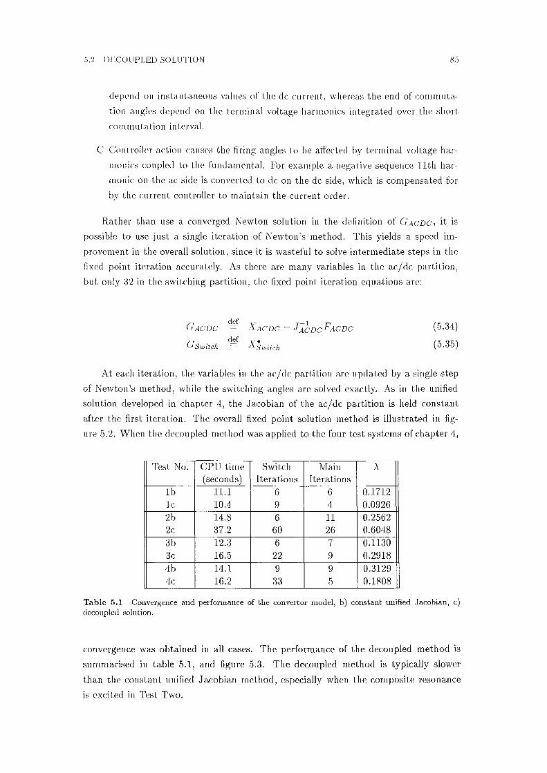
5.2 DECOUPLED SOLUTION 85
depend on instantaneous values of the de current, whereas the end of commuta
tion angles depend on the terminal volta.ge ha.rmonics integrated over the short
commutation interval.
C Controller action causes the firing angles to be affected by terminal voltage har
monics coupled to the fundamental. For example a negative sequence 11th har
monic on the ac side is converted to de on the de side, which is compensated for
by the current controller to maintain the current order.
Rather than use a converged Newton solution in the definition of GAcDC, it is
possible to use just a single iteration of Newton's method. This yields a speed im
provement in the overall solution, since it is wasteful to solve intermediate steps in the
fixed point iteration accurately. As there are many variables in the ac/dc partition,
but only 32 in the switching partition, the fixed point iteration equations a.re:
Gswitch def
Xswitch
(5.34)
(5.35)
At each iteration, the variables in the ac/dc partition are updated by a single step
of Newton's method, while the switching angles are solved exactly. As in the unified
solution developed in chapter 4, the Jacobian of the ac/dc partition is held constant
after the first iteration. The overall fixed point solution method is illustrated in fig
ure 5.2. When the decoupled method was applied to the four test systems of chapter 4,
Test No. CPU time Switch Main >. (seconds) Iterations Iterations
lb 11.1 6 6 0.1712 le 10.4 9 4 0.0926 2b 14.8 6 11 0.2562 2c 37.2 60 26 0.6048 3b 12.3 6 7 0.1130 3c 16.5 22 9 0.2918 4b 14.1 9 9 0.3129 4c 16.2 33 5 0.1808
Table 5.1 Convergence and perlormance of the convertor model, b) constant unified Jacobian, c) decoupled solution.
convergence was obtained in all cases. The performance of the decoupled method is
summarised in table 5.1, and figure 5.3. The decoupled method is typically slower
than the constant unified Jacobian method, especially when the composite resonance
is excited in Test Two.

86 CHAPTER 5 ALTERNATIVE I:MPLE:MENTATIONS
read in system data
calculate system constants
1/ solve switching system
calculate sparse J ACDC
bifactorise J ACDC
'----..i solve J ACDC Y=l},,_cDC
update variables with Y
(a) main harmonic system
NIT=O
calculate switching mismatches
calculate partitioned Jacobian
Kron reduce to 8 x 8 sub-matrix
bifactorise reduced system
solve for voltage, average delay angle, and average de current updates
back substitution to find switching angle updates
update primary voltages
(b) switching system
Figure 5.2 Overall algorithm for the fixed point solution.
One reason for the longer execution time of the decoupled method is the large
number of iterations of the switching system, as it is converged at every iteration of the
overall method. An improvement in execution time a.nd convergence, could possibly be
obtained by performing only one iteration of the switch system instead of converging it.
This approach has not been pursued because of the poor performance of the decoupled
method when applied to the NZ South Island system equivalent impedance.
When applied to the NZ South Island test system, the decoupled method diverges
if there is an even order harmonic voltage source in the ac system, converging only for
odd order harmonic sources. This divergence is related to the phase angle of the ac
system impedance, as a capacitive impedance leads to slower divergence, or even slow
convergence at the fourth harmonic. Making the ac system impedance balanced and
without interphase coupling does not affect the divergence of the decoupled method.
The decoupled method, to the extent that it has been developed here, is not robust
enough for general purpose use, as even order harmonic sources do occur in the ac
system.
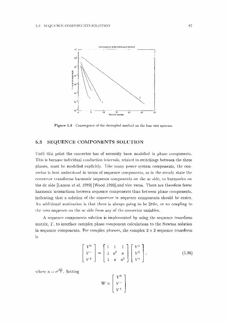
5.3 SEQUENCE COMPONENTS SOLUTION 87
Convergence of the Decoupled Method 10' ~-~--~--~--~--~--~
10--~-~--~--~--~--~-~ 0 5 10 15 20 25 30
Iteration number
Figure 5.3 Convergence of the decoupled method on the four test systems.
5.3 SEQUENCE COMPONENTS SOLUTION
Until this point the convertor has of necessity been modelled in phase components.
This is because individual conduction intervals, related to switchings between the three
phases, must be modelled explicitly. Like many power system components, the con
vertor is best understood in terms of sequence components, as in the steady state the
convertor transforms harmonic sequence components on the ac side, to harmonics on
the de side [Larson et al. 1989] [Wood 1993],and vice versa. There are therefore fewer
harmonic interactions between sequence components than between phase components,
indicating that a solution of the convertor in sequence components should be easier.
An additional motivation is that there is always going to be little, or no coupling to
the zero sequence on the ac side from any of the convertor variables.
A sequence components solution is implemented by using the sequence transform
matrix, T, to interface complex phase component calculations to the Newton solution
in sequence components. For complex phasors, the complex 3 X 3 sequence transform
is
[ ~] [ 1 1 1
][~:], 1 a2 a (5.36)
1 a a2
. 2,r where a= e3T. Setting
W= [ ~:]

88 CHAPTER 5 ALTERNATIVE IMPLEMENTATIONS
as the sequence components voltage yields T1V = TV, and -v = T- 1T1V. If a three phase
quantity has been decomposed in rea.l rectangular components, as in the .Jacobian
matrix, a real components sequence transform matrix, f, can be constructed:
1 ·o IR 1 0 1 0 1 0 va R
vo I 0 1 0 1 0 1 V_l
Vi 1 0 Ra2 -Ia2 Ra -Ia Vb TV= R =V v- 0 1 Ia2 Ra2 Ia Ra Vb
I I (5.37) v+ 1 0 Ra -Ia Ra2 -Ia2 VR R
v+ I 0 1 Ia Ra Ia2 Ra2 Vf
The existing phase components mismatch equations summarised in table 4.2 can
now be written as sequence component mismatches, in terms of the sequence com
ponents terminal voltage, using the sequence transform matrix. Sequence component
mismatches for the twelve pulse controlled rectifier are listed in table 5.2 below. The
equation No. of Eqns. functional notation Fw 300 W - T fis(T-1 W, ldk, Ido, Bf, ¢f, Bf,¢?) Fld 100 Idk - f19(T-l W, Jdk,ldo, Bf, cpf, Bf,¢?) Fj 6 ho(T-1 W, Idk, Bf, ¢r) Fj/ 6 h1 (T-l w, Jdk, Bf, cpf) Ff 6 fi4(Idk, Ida, Bf, ao) p-U
0 6 fi5(Idk, Ido, Bf, ao) Fs 1 h2 (T-1 W, Idk, Ido, Bf, Bf, ff, ¢f) Fao 1 h3(T_1-w, Idk, Ido, Bf, Bf, cpf, ¢f)
Table 5.2 Mismatches and variables for the 12 pulse rectifier with the terminal voltage in sequence components.
chain rule readily yields the modifications that must be made to the phase components
partial derivatives, to yield the sequence components partial derivatives:
[~;;] [DFw]
l):,;
[!:;] (5.38)
The resulting .Ja.cobia.11 matrix, calculated using the numerical perturbation rnethod,
is plotted in figure 5.5, a.nd shows a greater degree of sparsity. This is primarily due
to the a.bscrnce of any coupling betwe<)ll the 1/-ero sequence ac volta1;e hannonics and
any of the other convertor variables. In rnany cases, it would be possible to decouple
1/-ern sequence f'rorn the convertor rnodd completely, and solve the 1/-ero sequence termi-

5.4 CONCLUSION 89
na.l voltage directly after the convertor model had converged. This is because there is
usually no nonlinearity due to the convertor in the zero sequence.
Unbalance in the star-g/delta transformer however causes cross sequence coupling
m that transformer, with the result that a full three sequence solution is required.
This is illustrated in figure 5.6 of the Jacobian matrix, where the leakage reactance in
phase 'b' of the star-g/delta transformer has been increased from 0.18 to 0.30 per unit.
Coupling between zero sequence and all the other convertor variables is evident in this
case.
The overall sequence components solution algorithm is the same as that of fig
ure 4.8, with the switching system solved in phase components, and the harmonic
system solved in sequence components. Inspection of table 5.3 shows that convergence
of the sequence components method is usually slightly better than the phase compo
nents solution. Convergence on a step by step basis for the four test cases is plotted in
figure 5.4.
Test No. CPU time Switch Main >. (seconds) Iterations Iterations
lb 11.1 6 6 0.1712 ld 10.9 6 5 0.0851 26 14.8 6 11 0.2562 2d 15.0 6 12 0.2973 36 12.3 6 7 0.1130 3d 11.5 6 6 0.1056 46 14.1 9 9 0.3129 4d 13.4 9 8 0.2834
Table 5.3 Convergence and performance of the convertor model, b) constant unified Jacobian, d) Constant sequence components Jacobian.
Although the performance of the sequence components method is slightly better
than that of the phase components solution, it is not remarkably so. However the
storage requirements for the Jacobian elements are reduced by approximately 500 -
1000 elements for a solution up to the 50th harmonic. Sequence components modelling
may also have additional advantages when combined with synchronous machine models,
or a three sequence load flow.
5.4 CONCLUSION
Three alternative implementations of the convertor model have been investigated. One
of these, the polar coordinates implementation, was found to be unsuitable because
of poor conditioning of the Jacobian matrix, due to the large range of harmonic mag-

90 CHAPTER 5 ALTERNATIVE IMPLEMENTATIONS
101 Convergence ol the Sequence Components Method
10•
.c 10-'
~ E
! 10-• 0
e 0 C: I ~ 10-'
10 .... 4
10-• 0 2 4 6 8 10 12
Iteration number
Figm•e 5.4 Convergence of the constant sequence components Jacobian on the four test systems.
nitudes that are of interest. This conclusion was arrived at by forming analytical
expressions for the polar partial derivatives.
A decoupled method was implemented by partitioning each of the vectors of vari
ables and mismatch functions, into two sub-vectors associated with the switching sys
tem, and the harmonic interactions between the ac and de sides of the convertor. Such
a decoupling can be viewed as a fixed point iteration, for which there is a simple test on
convergence based upon the magnitudes of the partial derivatives of the iterating func
tions. These partial derivatives were calculated numerically for the CIGRE rectifier,
and found to contravene the convergence criteria. The decoupled method nevertheless
converges quite well for this system, except when the composite resonance is excited.
When applied to the hybrid CIGRE/NZ test system, the decoupled method was found
to diverge if even order harmonic sources were present in the ac system. The method
is therefore not robust enough for general purpose use.
The sequence components method was implemented by placing sequence/phase
transforms at selected stages of the phase components solution. This yielded a Jacobian
matrix with little or no coupling to the zero sequence, and therefore fewer terms in
the Jacobian. The sequence components method was found to yield slightly better
convergence than a solution in phase components. In the long term, the choice between
phase or sequence components modelling depends upon whichever is more efficient for
the modelling of the power system as a whole.

5.4 CONCLUSION
i::::: --~ :E 0
--~ ...., "@ u .,..., ....
. Q).
s ;::l z
LO ,-
Figure 5.5
91
O LO
gptn!UZlBW g~n1osqv
Numerically calculated sequence components .Jacobiall; 1:3 harmonics.

92
Ji .0 0
.. ~ >-,
crj u . ·c:
.......... <1.l.
s z
CHAPTER 5 ALTERNATIVE IMPLEMENTATIONS
I.!) 0 I.!) ..... gptll!Ullt?W ~1n1osqv
Figure 5,6 Numerically calculated sequence components Jacobian with unbalanced star-g/delta transformer; 13 harmonics.

Chapter 6
TENSOR LINEARISATION USING THE JACOBIAN
6.1 INTRODUCTION
A widely used and powerful technique for analysing nonlinear devices is to linearise
around an operating point. If the nonlinearity is a voltage-current relationship, the
linearisation yields an admittance. This type of linearisation is particularly relevant to
the convertor, as the convertor admittance can be combined with the ac and de system
admittances to analyse resonances, harmonic transfers, and harmonic magnification
factors. For example, [Bahrman et al. 1986) calculated the de side impedance of a
convertor, including the effect of ac side impedance at coupled harmonics. Dickmander
et al. [1994] analysed a GIC induced 5th harmonic resonance, and showed that the
resonance could only be explained by combining the impedance of the convertor at
the 5th harmonic with that of the ac system. The convertor impedance was in turn a
function of the de system impedance.
The linearisation of the convertor to a frequency dependent impedance is a simple,
yet powerful tool for solving ac/dc system interactions, that offers greater insight than
repeated numerical solutions of the interaction. The linearisation can be extended to
include coupling between harmonics on the ac and de sides of the convertor. This
was first proposed by Larson et al. (1989], with the linearisation calculated by many
small harmonic perturbations of a time domain simulation. More recently Wood and
Arrillaga [1995b] developed a frequency domain method for calculating the convertor
impedance directly.
The interactions between several nonlinearities can also be linearised, as in the anal
ysis of convertor transformer core saturation [Hammad 1992], [Chen et al. 1996). Rela
tionships other than between voltage and current have been linearised. Persson [1970],
Ferreira et al. [1987], and Wood and Arrillaga [1995a) have calculated relationships
between firing angle modulation and de current ripple, for modelling of the control
loop. Elimination of noncharacteristic harmonics by directly modulating the firing an
gle, has also required the linearisation of relationships between firing angle modulation
harmonics, and phase current harmonics [Farret and Freris 1990], [Hammad 1992).

94 CHAPTER 6 TENSOR LINEARISATION USING THE JACOBIAN
vVhen linearising general nonlinear devices to an equivalent impedance, representa
tion by a single complex number is not possible. This was noted by Semlyen et al. [1988],
who proposed the use of either complex or real valued matrices. The fact that the com
plex value of an impedance can depend upon the phase angle of the current flowing
through it, and still be linear, is not widely appreciated. Persson [1970] noted that
the linear transfer from firing angle modulation to direct current at the 6th harmonic
was phase dependent, and described a circle in the complex plane. The fact that this
applied to the convertor linearised impedance was noted by vVood 1 , and prompted an
investigation of the effect using three different convertor models [Wood et al. 1995].
Central to Newton's method for solving nonlinear systems is the Jacobian matrix,
which represents a linearisation of the system of equations at every iteration. Although
the Jacobian is typically held constant during the solution, it can be re-calculated at
convergence. In the context of the convertor model, it should therefore be possible
to use the Jacobian matrix to calculate equivalent impedances for the convertor, or
indeed any other linearised relationship. The advantage of calculating impedances in
this way is that the effect of control, switching instant variation, unbalance, and system
impedances are automatically taken into account.
Clearly the utility of this method increases as the generality of the Newton solution
is expanded. For example, a unified Newton solution of several ac systems connected
by de links, with load flow and transformer saturation represented, would enable the
direct calculation of any desired linear relationship from the Jacobian. In the remainder
of this chapter, methods for extracting impedances from the Jacobian matrix, and for
performing nodal analysis using phase dependent admittances are developed.
6.2 THE IMPEDANCE TENSOR
In this section a framework for linearising the convertor is established that is able to
account for the phase dependent nature of the convertor at some harmonics. This will
allow a linearised impedance representation of the convertor suitable for use in a real
components nodal analysis, or a complex conjugate type nodal analysis of the convertor
interaction with ac and de system linearisations.
Any power system component can be represented by a voltage controlled current
source: I= F(V), where I and V are vectors of harmonic phasors. The function F,
is a complex vector function, and may be non-linear, and non-analytic. If F is linear,
it may include linear cross-coupling between harmonics, and may be non-analytic,
ie harmonic cross coupling and phase dependence do not imply non-linearity in the
harmonic domain. It will be shown in section 6.3 that for harmonic perturbations less
than 0.2 p.u., the CIGRE current controlled rectifier is a good approximation to such
a device.
1 pers com, 1994

6.2 THE IMPEDANCE TENSOR 95
The linearised response of F to a single applied harmonic may be calculated by
taking the first partial derivatives in rectangular coordinates:
[ 21. I l [' f}_f'__a R _. /WR
- . EJF D..h ~
where F has been expanded into its component parts:
If the Cauchy-Rieman conditions
hold, then the matrix of partial derivatives is of the form
[ a -b ] , b a
(6.1)
(6.2)
(6.3)
(6.4)
which is a type of matrix isomorphic with the complex number field. The linearisation
then becomes
(6.5)
The complex admittance representation of a linearisation can therefore only be applied
to analytic current injections. Non-analytic injections are quite common, for example
in the load flow, I= S* /V"- for a P + jQ bus, which is also nonlinear. An example of
a linear, but nonanalytic injection would be:
This is linear, since if
Y1V1 + Y2Vt
Yi Vi+ Y2\/2*
aV1 + bVi
(6.6)
(G.7) (G.8)
(6.9)

96 CHAPTER 6 TENSOR LINEARISATION USING THE JACOBIAN
then
Y1 Vii+ Y2 V3*
Yi(aVi_ + bVi) + Y2(aV1 + bV2)*
aY1 V1 + bYi Vi+ aY2 Vt+ bY2 Vz'" afi + blz.
For such a source, the complex admittance is;
y I
V Y1V + Y2V*
V Y1 + IY2IL'.'. (L'.'.Y2 - 2L'.'.V)
(6.10)
(6.11)
(6.12)
(6.13)
(6.14)
(6.15)
(6.16)
The complex admittance twice traces a circular locus centered at Y1 in the clockwise
direction, as the angle of the applied voltage is varied through 21r. By the inverse
mapping, Z = f?"; also traces a circular locus, but in the anti-clockwise direction. Next,
it will be shown that any current injection, when linearised, can be written in the form
(6.17)
Expanding equation 6.17 into components,
(6.18)
Equating the matrices on the right hand sides of equations 6.18 and 6.1, the real and
imaginary parts of Y1 and Y2 are readily expressed in terms of the partial derivatives:
Yrn ! (aFR aF1) 2 av + av R I
Y11 1 ( aFr aFR) - -----2 avR a11r
Y2R 1 (aFR aF1) 2 avR a11r
Y21 = l(aFR aFr) 2 aVr + &VR (6.19)
For nodal analysis, the conjugate opera.tor is eliminated by treating conjugated volt
ages and currents as additional variables. The conjugation operator then introduces
a harmonic cross coupling term between the conjugated variables, and the linearised

6.2 THE IMPEDANCE TENSOR 97
admittance of any source can be written:
(6.20)
This is the nodal ana.lysis proposed by Semlyen et al. [1988], and used in the HDA
program. It has also been used to form ABCD parameter matrices relating harmonics
on the ac and de sides of the convertor [J alali and Lasseter 1991]. If F is non-analytic,
Y2 =/::. 0, and the complex admittance will be a circular locus. For positive frequency
nodal analysis, the real matrix of partial derivatives is retained, and is henceforth called
the admittance or impedance tensor:
y = [ Yn Y21
Y12
Y22 (6.21)
The nodal analysis is then performed in real components using a Cartesian vector repre
sentation of voltage and current phasors on the Argand plane, and a second rank tensor
representation of admittances and impedances. Tensors are widely used in physics to
represent a relationship between vectors that is invariant under rotation of the coordi
nate axes [Arfkin 1985]. In this case, the coordinate axes are the real and imaginary
components of the complex voltage phasor, which rotate under a shift in phase refer
ence. The components of the voltage therefore transform like the elements of a vector
under this rotation. Since the current is a vector function of the voltage, the matrix of
partial derivatives can be written as the direct product of the gradient operator with
the current vector, yielding a second rank tensor
- "T Y=VI, (6.22)
Although the elements of the tensor admittance are modified by a change in phase
reference, they transform in such a way that the relationship described by the tensor,
dependence of current on voltage, is invariant. When the tensor admittance is extended
to three phases and multiple harmonics, the dimension will be 6nh, but the rank of the
tensor will still be two.
Given an admittance tensor Y, the impedance tensor is
z = y-i = [ z11 z12 l Z21 Z22
(6.23)
The impedance tensor corresponds to a circular impedance locus on the complex plane,
of radius r, x-position a, y-position b, and rotation ~(. The rotation of the impedance
locus is defined to be the angular position on the circular locus corresponding to an
applied current of phase 0. These quantities are illustrated in figure 6.1. In Appendix D,

98 CHAPTER 6 TENSOR LINEARISATION USING THE JACOBIAN
b
I I I I '
:,'-Y -------_J' -_,_ -- --
)). a Real
Figure 6,1 Complex impedance locus for an impedance tensor. The locus point rotates counter clockwise twice, starting from the angle "'(, as the current injection ranges in angle from O to 2rr.
the parameters of the impedance circle are derived entirely in terms of the tensor
components, and are listed below.
1 (6.24) a 2(zu + z22)
b 1 2(-z12 + Z21) (6.25)
1 1' 2✓(zu - z22)2 + (z12 + z21)2 (6.26)
' t -1 Z12 + Z21 (6.27) an
Z22 - zu
Since the impedance tensor is a matrix, it may not be invertible, in which case the
determinant is zero. However
a2 + b2 - r2 1 [(zu + z22) 2 + (-z12 + z2i)2 - (zu - z22) 2 - (z12 + z21) 2]
Zn Z22 - Z12z21
det(Z), (6.28)
and the tensor is invertible if and only if the complex circular locus does not intersect the
origin. The x-axis intercepts of the circular locus correspond to a resistive impedance,
so that
Zl= RI. (6.29)
The eigenvalues of Z are therefore the values of resistance where the locus intersects

6.3 CALCULATION OF THE CONVERTOR IMPEDANCE
the x-axis. The characteristic equation is
(z11 - R) z12
z21 (z22 - R)
0,
gg
(6.:30)
(6.:31)
which is a quadratic in R, and it is easy to show that a real solution for R is only
possible if r 2 > b2 , ie the circular locus is close enough to the x-axis. If the x-axis
intercepts are considered as being a type of resonance, then the eigenvectors of Z are
those currents that have the correct angle to excite the resonance.
6.3 CALCULATION OF THE CONVERTOR IMPEDANCE
In general the convertor impedance for small distortions will be phase dependent, and
therefore best represented by a tensor. The impedance tensor can be directly calcu
lated from the convertor Jacobian, since the Jacobian is a linearisation of the convertor
around an operating point. Firstly however, the phase and magnitude dependence of
the convertor complex impedance to an applied harmonic voltage distortion is investi
gated by applying a variety of small harmonic distortions to the convertor terminal.
6.3.l Perturbation Analysis
An approximation to the convertor impedance to small harmonic distortions applied
to the ac terminal can be determined by solving the convertor model for perturbations
around an initial solution. For example, to solve the 7th harmonic positive sequence
impedance, the convertor base case is first solved (Test One in Chapter 4). A sequence
transform is then applied to the 7th harmonic voltage and phase current at the ac
terminal to yield base values:
(6.32)
(6.33)
Next, a small positive sequence 7th harmonic voltage source is added to the ac system
Thevenin voltage source, and the convertor model is rc)-converged. The perturbed
positive sequence 7th harmonic ac terminal quantities are then calculated, as above:
v+ 7p
r:J; [TVir]+
[Thp]+
((U4)
(6.:35)
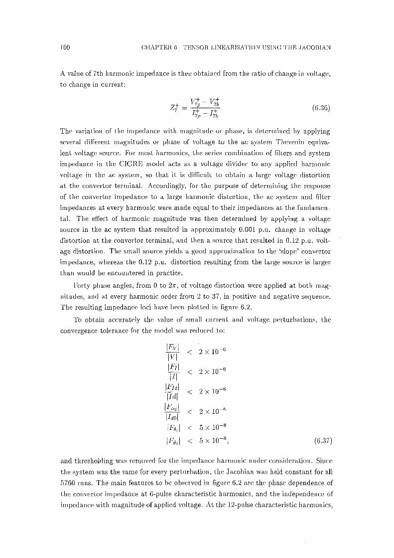
100 CHAPTER 6 TENSOR LINEARISATION USING THE JACOBIAN
A value of 7th harmonic impedance is then obtained from the ratio of change in voltage,
to change in current:
(6.:36)
The variation of the impedance with magnitude or phase, is determined by applying
several different magnitudes or phase of voltage to the ac system Thevenin equiva
lent voltage source. For most harmonics, the series combination of filters and system
impedance in the CIGRE model acts as a voltage divider to any applied harmonic
voltage in the ac system, so that it is difficult to obtain a large voltage distortion
at the convertor terminal. Accordingly, for the purpose of determining the response
of the convertor impedance to a large harmonic distortion, the ac system and filter
impedances a.t every harmonic were made equal to their impedances at the fundamen
tal. The effect of harmonic magnitude was then determined by applying a voltage
source in the ac system that resulted in approximately 0.001 p.u. change in voltage
distortion at the convertor terminal, and then a source that resulted in 0.12 p.u. volt
age distortion. The small source yields a good approximation to the 'slope' convertor
impedance, whereas the 0.12 p.u. distortion resulting from the large source is larger
than would be encountered in practice.
Forty phase angles, from 0 to 21r, of voltage distortion were applied at both mag
nitudes, and at every harmonic order from 2 to :37, in positive and negative sequence.
The resulting impedance loci have been plotted in figure 6.2.
To obtain accurately the value of small current and voltage perturbations, the
convergence tolerance for the model was reduced to:
IFvl < 2 X 10⁻⁶
WI IF1I < 2 X 10⁻⁶
III IF/di < 2 X 10⁻⁶
IId/ !Fool < 2 X 10⁻⁶
II do/ /Fe;/ < 5 X 10-S
/F¢,;I < 5 X 10⁻⁸ , ( 6.:37)
and thresholding was removed for the impedance harmonic under consideration. Since
the system was the same for every perturbation, the Jacobian was held constant for all
5760 runs. The main features to be observed in figure 6.2 are the phase dependence of
the convertor impedance at 6-pulse characteristic harmonics, and the independence of
impedance with magnitude of applied voltage. At the 12-pulse characteristic harmonics,

6.3 CALCULATION OF THE CONVERTOR Ii\!IPEDANCE
Convertor impedance
~r:;~tive sequence negaative sequenc:37
. EB34
~ • ®33 o - 12 % perturbation
en E ..c 0 I = t::
co 0.
i::' co C
2000
1500
., 1000
EB32 + - 0.1 % perturbation
es1 EB30
7
0 200 400 600 0 Real part (ohms)
• EB32
EB31
EB30
EB29
EB28
• EB27
• EB26
5
~~6~1 .9 0. 18
17
EB
EB15
200
101
5
400
Figure 6.2 Dependence of convertor impedances on magnitude of applied voltage perturbation.

102 CHAPTER 6 TENSOR LINEARISATION USING THE JACOBIAN
a large value of distortion leads to an epicyclic phase dependent locus, due to the
coupling of these harmonics to the average de current, and hence control action. At
all other harmonics and sequences, the convertor impedance is essentially completely
linear over the ra.nge of magnitudes likely to be encountered. In practice, there will
also be filters at the characteristic and high order harmonics, and high levels of voltage
distortion will not be encountered.
Despite a uniform progression of voltage phase angles applied to the 5th and 7th
harmonics, the associated circular loci display a clustering of impedance points near
the origin. This is a consequence of the perturbation method used, rather than the
impedance itself, and is best explained by considering the locus of the returned current
perturbations, as plotted in figure 6.3 for the positive sequence 7th harmonic.
Locus of Positive Sequence 7th Harmonic Current . . . . . . . ' . . . . . . . . . . . . . . . . .
-800 -600 -400 -200 0 200 400 600 800 Real Part (mA)
Figme 6.3 ....,\\
Locus of the perturbed •fifth harmonic current.
As the applied voltage phase progresses uniformly through 271', the returned cur
rent is determined by a uniform double rotation around the admittance locus. The
admittance locus is not concentric with the origin, and so the returned current is small
only for those few points on the admittance locus close to the origin. This results in
the clustering of points on the extrema of the elliptical current locus. When points
on the impedance locus are calculated, this clustering effect is compounded by the
radial distance from the origin on the impedance plane, since the current locus is clus
tered at large values of current, which correspond to small impedances. If the voltage
perturbation method is used to calculate the admittance locus instead, the points are
equi-spaced. If the impedance locus is centered a long way from the origin, relative to
the radius of the locus, the clustering is insignificant.
In relation to the earlier discussion on phase dependence, it is evident that the
convertor impedance can be described by complex numbers at all harmonics, apart
from h = 6n ± l. At these harmonics the impedance should be a tensor representation,
or a coupling to the conjugate of the applied voltage. The generation of harmonic
6.3 CALCULATION OF THE CONVERTOR IMPEDANCE 103
currents by the convertor related to the conjugate of an applied voltage distortion
is predicted by the modulation theory ana.lysis of Wood and Arrillaga [199.5b]. The
impedance of the convertor ls calculated in this model by superimposing the effect of
several small amplitude waveform distortion transfers, each calculated by modulation
theory. Although this model predicts many relationships involving multiples of the
modulation frequency, these higher order terms are very small, and it suffices for a
qualitative understanding of the convertor impedance to consider only the relationships
described below.
Modulation Theory of the Impedance The application of either a positive se
quence harmonic voltage of order (k + 1) angle f>, or a negative sequence harmonic
(k - l)Lf> on the ac side of the convertor is directly transferred to a de side voltage
kL(a1 + f>) and a small (12 - k)L(a2 - f>), where Cl£ is a constant angle. If k = 6 then
the first reflected term, (12 - k), is at the same harmonic, but phase conjugated. This
mechanism of phase conjugation occurs quite generally for all the distortion transfers
through the convertor. The de ripple at harmonic k, resulting from the voltage ripple,
will be transferred to the a.c side currents (k + l)L(a3 + f>) in positive sequence, and
(k-l)L(a4+f>) in negative sequence. There will also be ac side currents (ll-k)L(a5-J)
in positive sequence, and (13 - k)L(a6 - f>) in negative sequence. The reflected terms,
(11 - k) and (13 - k), are very small, but demonstrate one mechanism whereby there
is a phase conjugation of applied voltage to returned current on the ac side.
Commutation Period Modulation The application of harmonic voltage orders of
either ( k+ 1) Lf> in positive sequence, or ( k-1) Lf> in negative sequence on the ac side will
directly modulate the end of commutation angles at harmonic kL( a7 + f>). This has a
very significant effect on ac side impedances, since the full de current will be modulated.
The encl of commutation modulation leads to a range of modulation products on the ac
side, including the harmonic orders (k+l)L(a8 +f>) in positive sequence, (k-l)L(a9 +f>)
in negative sequence, (11 - k)L(a10 - f>) in negative sequence, and (13 - k)L(au - f>)
in positive sequence. The reflected terms in this case are significant, and are scaled
by the product of two sine functions: sinc(k/t/2)sinc(m/t/4), where m = 1, 11, 13, 23 ...
Setting k = G, indicates tha.t the 5th negative, and 7th positive sequence impedances
of the convertor arc substantially phase dependent. If a 6th positive sequence voltage
is applied to the convertor there will be a negative sequence current returned, and vice
versa.. A similar analysis holds for a.II G-pulse order harmonics, reflecting as appropriate
from higher order multiples ol' the modulating frequency.
Having established that the convertor impedance is magnitude independent, and
best represented by a tensor at particular harmonics, it is not necessary to calculate
the complex impeda.nce for a full 2,r of applied voltage distortions. In !'a.ct, just two
perturbations yield four equations in the four unknown tensor elements. However the

104 CHAPTER 6 TENSOR LINEARISATION USING THE JACOBIAN
perturbation method is essentially a numerical partial differentiation, rife with poten
tial problems. For example, it is difficult to know if the perturbation is definitely small
enough, and whether the convergence tolerance specified has yielded suitably accurate
data points. In the next section, the Jacobian matrix is modified to yield directly any
desired tensor relationship. Anticipating this result, figure 6.14 is a comparison of the
CIGRE rectifier impedance loci calculated analyticaUy from the Jacobian (continuous
circles), and by perturbation (data points on circles), for every harmonic order from
2 to 37 in positive and negative sequence. The perturbation calculation of the con
vertor impedance has been further intervalidated against perturbation of an EMTDC
model, and a direct 6-port analytic calculation using the above described analytic model
in (Wood et al. 1995).
6.3.2 The Lattice Tensor
Several authors, most notably [Larson et al. 1989), have noted that from the point of
view of the ac system, the convertor presents a stable and quite linear set of interrela
tionships between harmonics and sequences. For example, the application of a positive
sequence voltage distortion at harmonic order k + 1, leads to the injection of harmonic
currents (11 ± k), (23 ± k), etc in negative sequence, and (1 ± k), (13 ± k), (25 ± k)
etc in positive sequence. The difference terms a.re always phase conjugated, unless the
harmonic would be negative, in which case the sequence is reversed. In fact the analysis
of (Wood and Arrillaga 1995a) predicts many other multiple reflections that usually,
but not always, decay with order (for example 12rn ± nk ± 1). This 'numerology of the
convertor' is succinctly summarised by a lattice-like diagram of connections between
harmonics and sequences, as shown in figure 6.4, for n = l. Points on figure 6.4 marked with a'+', can be represented by a complex admittance.
Points marked by a 'o' represent couplings between positive and negative harmonics,
and can be represented either by a circular admittance locus centered on the origin in
the complex admittance plane, or by a tensor. Points with both markers, at lattice
vertices, indicate that the total current returned consists of two components, related
to the voltage applied, and its conjugate. Such points correspond to a circular locus
in the complex plane shifted away from the origin. Figure 6.14 is a plot of impedances
along the diagonal of figure 6.4, with circular loci occurring at the 6-pulse characteristic
harmonics. Also marked on figure 6.4 is the special case of a sixth harmonic positive
sequence distortion. A current is returned at the same harmonic in both positive and
negative sequence, and it can be seen that the convertor transforms between positive
and negative sequence for aU harmonics k = 6n.
If the convertor is unbalanced, or there are large harmonic distortions, the cross
coupling lattice will fill in to some extent, especially at low order harmonics. There
will also be current injections related to the conjugate of applied harmonic voltages at

6.3 CALCULATION OF THE CONVERTOR IMPEDANCE
+ve Seq.
0 6 10 20 0 10 Applied Voltage Distortion
20 30
Q)
'i
er Q)
Cf)
Q)
'j:
105
Figure 6.4 Principle harmonic currents returned by a twelve pulse convertor in response to an applied voltage distortion. '+'- current phase related to phase of applied voltage, 'o' - current phase related to conjugate of applied voltage.
most harmonics. In general then, the lattice is most accurately represented by a large
lattice tensor, of second rank, but of size 4nh X 4nh (unless there is coupling to the
zero sequence). The lattice tensor can be calculated from the Jacobian matrix by first
noting that partial derivatives of the voltage mismatch are of the form:
aFv ax
av ax
aJ18 ax (6.38)
where !18 is the calculated terminal voltage, obtained by injecting the phase currents
into the ac system impedance:
consequently
aJ18 ax [y ]_1 a[Ij + I#]
cc k ax
(6.39)
(6.40)
Those rows of the Jacobian that contain partial derivatives of the voltage mismatch
are therefore easily modified to contain partial derivatives of the phase currents with
respect to the system variables ( terminal voltage, de current, switching angles). The

106 CHAPTER 6 TENSOR LINEARISATION USIKG THE JACOBIA='J
matrix equation defined by the new matrix, .P, is now:
61 E!I 8I E!I E!I ..ill_ eiV av 8Jd 8¢ 80 8ao
6Fu DF1d DFJd DF1d EIFJd DF1c1
61 d av Dk t;Jq, Ei0 Bao DF1, /j DF1 DF1, (6.41) 6Fo
¢ 6¢ av E!Jd 75¢ 80 Dao
6F0 DFe E!Fe E!Fe E!Fe DFe 60 av 8Jd 8¢ 80 Doo
6Fao DF9 o DFao DFao DFao E!Fao 6ao av E!Jd El¢, E/0 Elao
At the convertor solution, all the mismatches are equal to zero. vVhen a harmonic
voltage perturbation is applied, it is required that all the mismatches in equation 6.41
remain zero, ie 6F = 0. Partitioning .J' around l, and V, equation 6.41 ca.n be written:
[ 61 l [ A B l [ 6 V l 0 C D 6X'
(6.42)
Eliminating 6X':
(6.43)
The large matrix D is not actually inverted, instead columns, Yi of n- 1c are
obtained from solutions to the linear system
(6.44)
where Ci are columns of C. This procedure is much faster as it avoids the matrix
multiplication a.nd storage of n-1 , and the LU decomposition of D is only calculated
once.
Since l and V have been decomposed into real valued components, the matrix
Yep = A - BD- 1C is a second rank tensor, It is actually a phase components version
of the lattice network, connecting harmonics and phases, rather than harmonics and
sequences. The phase components cross coupling tensor has been plotted in figure 6.5,
for harmonic interactions up to the 21st harmonic. Only admittances larger than 0.005
p.u. have been retained, and only magnitudes have been plotted. The tensor is 126
elements square (2 x 3 X 21).
Application of the sequence components transform yields the same tensor in se
quence components, plotted in figure 6.6. In sequence components the lattice tensor
clearly contains far fewer terms, and the zero sequence part has been diagonalized by
the transform. The lattice tensor has also been calculated around the operating points
of Test 2 in figure 6.7, and Test 3 in figure 6.8. The presence of 2nd harmonic terminal
voltage distortion in figure 6.7 has increased the number of significant cross harmonic
couplings. As expected, unbalance of the star-g/delta transformer in figure 6.8 has re-

6.3 CALCULATION OF THE CONVERTOR IMPEDANCE
,:... ·O
'·········.-'C/)·· ·C
(I)
1-(1) u .. E' <1l
...J ............. 2.1.
C (I) C 0 Q.
E ..... ·.·8
·. (I) . CJ) ·.!1l aC a..
l{) 'Sf' Cf) N
('n ·d) epnJ!UBBV'J e1n1osqv 0 ,...
Figure 6.5 Phase components lattice tensor calculated at the solution of Test 1.
107
0 c3 (I)
> (I) 0) <1l ~ 0 > "O -~ 0. Q. <(
0
0
,_
~ (I)
> -C
~ ::J ()
"O (I) C ,_ ::J
m a:
108 CHAPTER 6 TENSOR LINEARISATION USING THE JACOBIAN
sulted in substantial coupling to the zero sequence, due to sequence transformation by
that transformer. As in Test 2, the unequal commutation periods and voltage samples
lead to many more significant admittance terms.
Ignoring now the zero sequence, since there is usually little or no coupling to it
in the convertor, the lattice diagram of figure. 6.4 is verified against the lattice tensor
calculated above. Each'+' or 'o' in figure 6.4 represents four real elements in the lattice
tensor, corresponding to variations in the real and imaginary parts of the returned
current distortion in response to variations in the real and imaginary parts of the
applied voltage distortion ( which may be at a different harmonic and sequence). These
four elements constitute a tensor cross coupling term that can be represented by a
circular locus in the complex admittance plane. By considering sequentially every such
cross coupling tensor, figure 6.9 is the result of applying the following plotting rules to
the lattice tensor calculated at the solution of Test 1:
1. If the center of the locus is farther than 0.005 p.u. from the origin, plot a'+'.
2. If the radius of the circular locus is greater than 0.005, plot a 'o'.
3. If a'+' has been plotted, and the radius is greater than 1 % of the distance of the
center of the locus from the origin, plot a 'o' as well.
4. If an 'o' has been plotted, and the distance of the center of the locus from the
origin is greater than 1% of the radius of the locus, plot a'+' as well.
The purpose of the plotting rules is to sift out very small admittances, but to still
show the nature of admittances that have been retained. The result is a classification
of the crosscoupling tensors into direct '+', and phase conjugating 'o' admittances,
that essentially recreates the lattice diagram of figure 6.4 in figure 6.9. However, if the
same process is applied to the lattice tensor calculated at the solution of Test 2, the
result is a lattice diagram, figure 6.10, with a considerable amount of fill-in. A more
realistic case is plotted in figure 6.11, where the ac system source was distorted by 1%
negative sequence fundamental, resulting in 0.8% negative sequence fundamental at
the convertor ac terminal. The conclusion to be drawn is that the lattice diagram is
only valid in balanced, undistorted conditions.
The lattice tensor can be used to form a Norton equivalent for the convertor.
However given that the convertor model developed in Chapters 3 to 5 converges rapidly,
it is not necessary to approximate the convertor by a linearised equivalent in order to
solve ac system interactions.
Several authors have proposed the use of ABCD parameter matrices to characterise
the harmonic interaction of the ac and de systems, ie
(6.45)
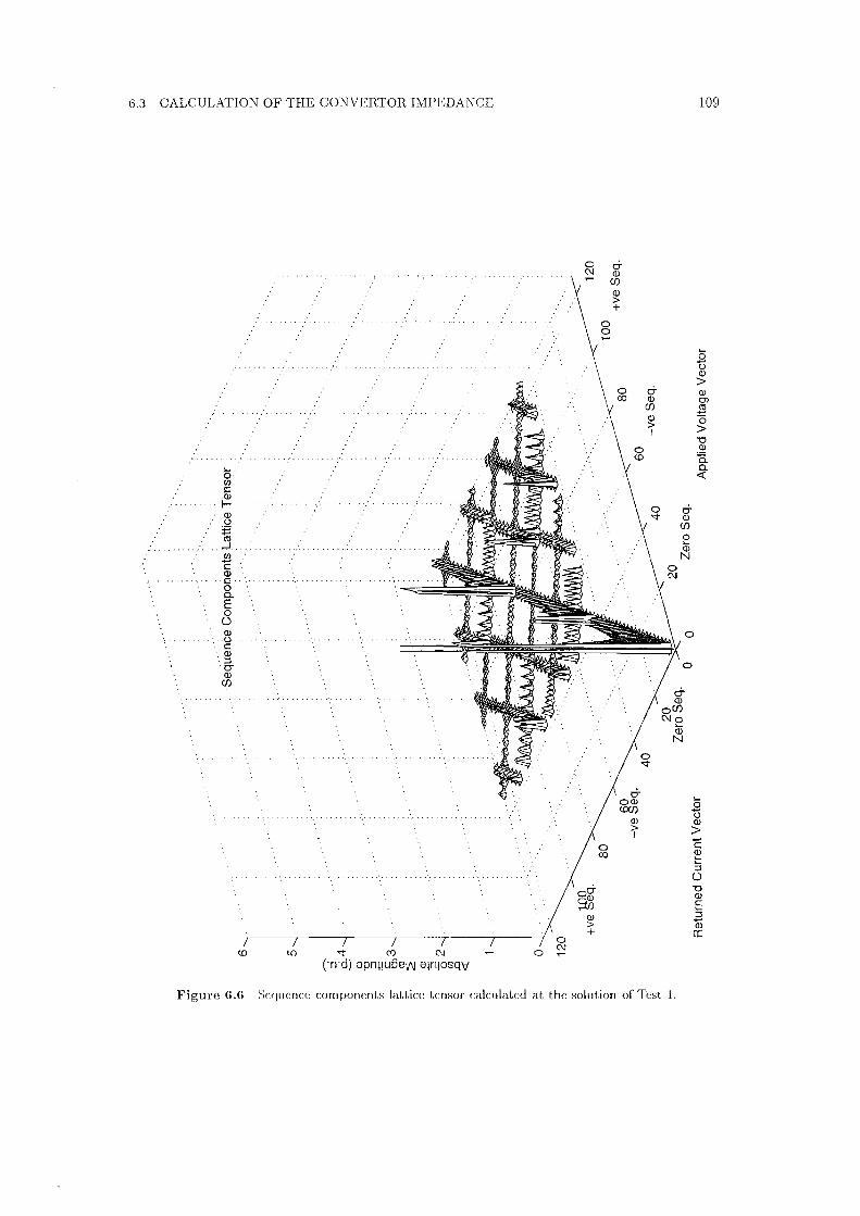
6.3 CALCULATION OF THE CONVERTOR IMPEDANCE
Q ... en C
.<I) .. ·.I
Q) u
~ . ,..,.I.
en c Q) .
··C·· 0 0. E 0 0 Q)
···U· C
. Q) . ::i ·.rr
Q) (f')
I.[) 'SI" C') N ,-
('n·d) apnJ!U5Blf'J a1n1osqv
0
0 N ,-
0 c:i-N Ql
0 co
ad-~
Q)
> +
(f') Q)
> +
d-OQl (£(/)
Q)
> I
109
... .8 u Q)
> c:i- Q) Q) 0)
(f') .s Q) 0 t >
"O .~ C. 0. <(
0
0
d-Q)
OU) No ,._
Q)
N
0 t5 Q)
> -C Q) ... ... ::i 0 "O Q) C :i -Q)
r.r:
Figure 6.6 Sequence components lattice tensor calculated at the solution of Test 1.

llO CHAPTER 6 TENSOR LINEARISATION USING THE JACOBIAN
(\J
.U). Q)
f-
c5 (/) C
···········'.·~·•·
·.~ ·::a .:5
co I!) '<I" CV) (\J ,- 0 ('n·d) epn11u6eV1J e1n1osqv
Figure 6. 7 Sequence components lattice tensor calculated at the solution of Test 2.
,._ .8 u Q)
> Q) 0)
~ 0 > "O -~ 0. Cl. <(
.... ~ Q)
> -C ~ :5 0 "O Q) C .... ::i 1i5 a:

6.3 CALCULATION OF THE COXVERTOR J"MPEDANCE
(I)
t5 Q)
f-..: 0 (f) C Q)
'·.•f-. Q) u
·:P ·1a .:..J
<:t' C') N ,-
('n·d) apni1ufle1111 ain1osqv 0
0 N
Figu1·e 6.8 Sequence cornponcntH lattice tensor calculated at the solution of Tesl :.!.
0 Qi N
111
.... .8 u Q)
> Q) 0)
.8 0 > "O .~ 0.. 0.. <(
0
0
.... 0 t5 Q)
> c ~ :::l ()
"O (1) C .... ::J Ql a:
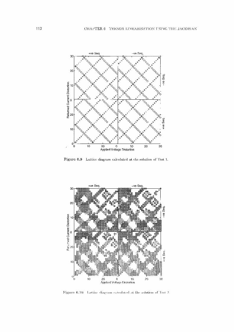
112
C: ~o ::, 0 'O (1)
E ::, a, 20 a:
CHAPTER 6 TENSOR LINEARISATION USING THE JACOBIAN
+ve Seq. -ve Seq.
(1)
t
'.!; +
20 30
Figure 6.9 Lattice diagram calculated at the solution of Test 1.
C:
-.@ 10
tl i5 C: ~o ::, 0 'O (1)
E ::, a, 20 a:
+ve Seq.
10
-ve Seq.
20 0 10 Applied Voltage Distortion
& (1)
(/)
(1) > I
& (1)
(/)
(1)
> +
20 30
Figure G.10 LaUic:e diagram c:alc:11!ated at the solution of Test 2.

6.3 CALCULATION OF THE CO:-TVERTOR IJ\1I PEDA:NCE
+ve Seq. -ve Seq.
30
& (!)
(J)
~ I
& (!)
(J)
113
Figure 6.11 Lattice diagram calculated at a solution with 0.85% negative sequence fundamental voltage distortion at the convertor terminal
with the ABDC parameters calculated by means of the perturbation of time domain
simulations, or perturbation of a switching function approach. The ABCD matrix
( or tensor in positive frequency analysis), can be calculated directly from the Jacobian
matrix by modifying the de mismatch derivatives to be derivatives of the de voltage, and
then performing a Kron reduction to eliminate the switching angle perturbations, as
for the lattice tensor above. Once again however, this is of limited use in ac/dc system
harmonic analysis, since the full interaction can be solved quickly by the convertor
model.
In the next section, the lattice tensor is combined with the ac system tensor admit
tance, and then used to calculate the impedance of the convertor at selected harmonics
and sequences.
6.3.3 Derivation of the Convertor Impedance by Kron Reduction
Calculation of equivalent, or driving point impedances is widely used in system analysis
to derive Norton or Thevenin equivalents. For example, the nodal analysis method is
used in harmonic penetration and load flow programs, with each node corresponding
to a physical node in phase components. When a Kron reduction is applied to a
complex admittance matrix, the result is a matrix of reduced size, fully representing
the interaction between sources connected to the remaining nodes,
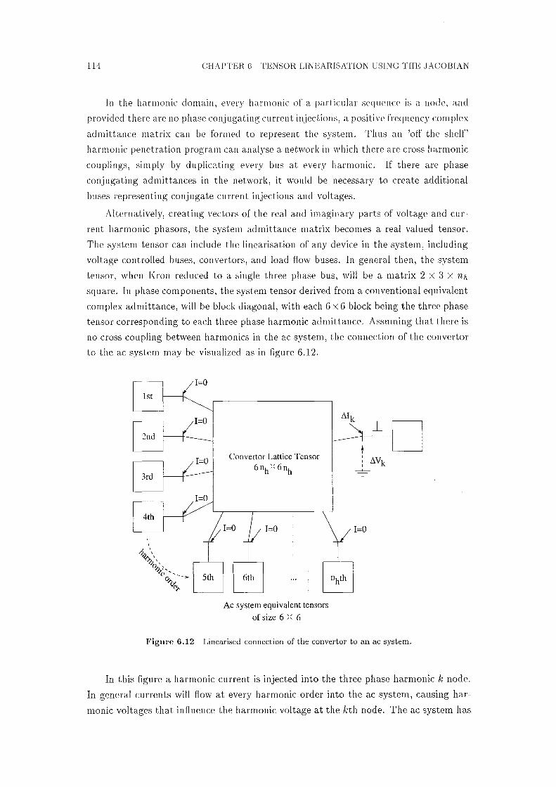
114 CHAPTER 6 TENSOR LINEARISATION USING THE JACOBIAN
In the harmonic domain, every harmonic of a particular sequence is a node, and
provided there are no phase conjugating current injections, a positive frequency complex
admittance matrix can be formed to represent the system. Thus an 'off the shelf'
harmonic penetration program can analyse a network in which there are cross harmonic
couplings, simply by duplicating every bus a.t every harmonic. If there are phase
conjugating admittances in the network, it would be necessary to create additional
buses representing conjugate current injections and voltages.
Alternatively, creating vectors of the real and imaginary parts of voltage and cur
rent harmonic phasors, the system admittance matrix becomes a real valued tensor.
The system tensor can include the linearisation of any device in the system, including
voltage controlled buses, convertors, and load flow buses. In general then, the system
tensor, when Kron reduced to a single three phase bus, will be a matrix 2 X 3 X nh
square. In phase components, the system tensor derived from a conventional equivalent
complex admittance, will be block diagonal, with each 6 x 6 block being the three phase
tensor corresponding to each three phase harmonic admittance. Assuming that there is
no cross coupling between harmonics in the ac system, the connection of the convertor
to the ac system may be visualized as in figure 6.12.
1st
2nd
3rd
4th
5th
Convertor Lattice Tensor 6nh)( 6nh
1=0 1=0
6th
Ac system equivalent tensors
of size 6 )( 6
1=0
Figure 6.12 Linearised connection of the convertor to an ac system.
In this figure a harmonic current is injected into the three phase harmonic k node.
In genera.I currents will flow at every harmonic order into the ac system, causing har
monic voltages that influence the harmonic voltage at the kth node. The ac system has

6.3 CALGCLATIO:\f OF THE CONVERTOR IMPEDANCE 11.S
been disconnected from the convertor at the kth harmonic, since we 'Want to calculate
the convertor impedance only. The nodal equation corresponding to this scenario is:
[ li, l [ A+ diag(}7sys)
C (6.46)
The matrices A, B, C, and D are obtained by moving the six rows and columns
of the lattice tensor associated with harmonic order k, to the end of the tensor, and
then partitioning off these last six rows and columns. The matrix A is therefore of size
6(nh - 1) x 6(nh - 1). A current injected at any of the three phase harmonic nodes
marked in figure 6.12 will see the system and convertor tensor admittances in parallel,
consequently the system 6 X 6 equivalent admittance tensors are added as a block
diagonal matrix to partition A of the convertor lattice tensor. The system admittance
at the kth harmonic has been disconnected frorn the convertor, and so is not added to
the D partition.
Applying the Kron reduction to equation 6.46, yields the equivalent 6 x 6, kth
harmonic three phase tensor admittance at the convertor ac terminal:
(D - C(A + diag(Ysys))- 1 B)fl Vi (6.47)
( 6.48)
This tensor admittance is a linearisation of the convertor response to applied kth har
monic three phase voltage perturbations, and includes the effect of control, switching
angle variation, and coupling to the ac and de systems at other harmonics. Once again,
the large matrix A+ diag(Ysys) is not actually inverted, but rather bifactorised to LU
form, and then columns of (A+ diag(Ysys))- 1 B are obtained by solving the linear
system
(A+ diag(Ysys))Yi = B(:, i), (6.49)
where the Yi are the columns of (A+ diag(Ysys))- 1 B. Sequence transforming Yr:k, it
is possible to apply another Kron reduction to obtain a single sequence equivalent.
The situation here is more complicated than in figure 6.12, as in general the ac system
admittance at a particular harmonic will contain intersequence coupling. The situation
is illustrated in figure 6. 1:3, where we wish to find the equivalent positive sequence 7th
harmonic admittance of the convertor, under the assumption that both the convertor
and ac system convertor transform between sequences at this harmonic. The following
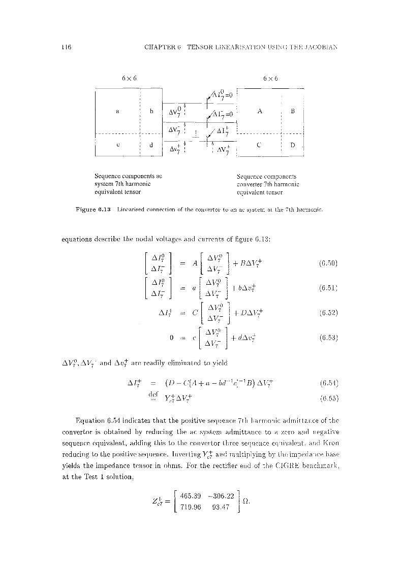
116 CHAPTER 6 TENSOR LINEARISATION USING THE JACOBIAN
6x6 6x6
a b
I
------------~------'
C d
Sequence components ac system 7th hatmonic equivalent tensor
!J.V~:
tJ.v:, J_
Ii+ I V7 I
0 L1I 7 =0
foC7=0
/ !J.I;
!J.V+ 7
A
I
I
B
____________ J _____ _
I I
C I D
Sequence components converter 7th harmonic equivalent tensor
Figure 6,13 Linearised connection of the convertor to an ac system at the 7th harmonic.
equations describe the nodal voltages and currents of figure 6.13:
- [ fll~ l fll7
0
fl Vl, fl v7- and fl vf are readily eliminated to yield
(6.50)
(6.51)
(6.52)
(6.53)
(6.54)
(6.55)
Equation 6.54 indicates that the positive sequence 7th harmonic admittance of the
convertor is obtained by reducing the ac system admittance to a zero and negative
sequence equivalent, adding this to the convertor three sequence equivalent, and Kron
reducing to the positive sequence. Inverting YJ and multiplying by the impedance base
yields the impedance tensor in ohms. For the rectifier end of the CIGRE benchmark,
at the Test 1 solution,
z+ = [ 465.39 -306.22 ] n. c7 719.96 93.47

6.3 CALCULATION OF THE CONVERTOR IMPEDANCE 117
Repeating these calculations for every harmonic from 2 to 37, in positive and negative
sequence, the resulting circular impedance loci have been plotted in figure 6.14. Data.
points obtained by the perturbation method have also been plotted on this diagram.
The method developed here for calculating the convertor impedance is somewhat
circuitous, as it is not necessary to first calculate the lattice tensor, and then reduce
to a single harmonic equivalent. For example to calculate the 7th harmonic impedance
from the .J a.cobia.11, it would be possible to retain voltage mismatches for every harmonic
except the 7th, and then Kron reduce the .Jacobian to the 7th harmonic partition.
This method would be faster for calculating a. single harmonic impedance, but slower
for calculating many. Another method would be to repeatedly Kron reduce to small
lattice tensors covering a limited range of frequencies. Typically we a.re interested
in harmonics below the 11th, and could therefore retain voltage mismatches in the
.Jacobian above the 10th harmonic, reduce to a. ten harmonic lattice tensor, and then
sequentially reduce this tensor to harmonic equivalents. This method would offer a.
(49/9) 3 = 161-fold improvement in speed for the calculation of ea.ch harmonic, after the
initial calculation of the lattice tensor, but would give the same results. Nevertheless,
by obtaining exact agreement with the perturbation method, the lattice tensor itself,
and the nodal analysis utilizing that tensor, have been validated.
In Chapter 7 the possibility of extending the convertor model to integrate several
a.c systems, loadflows, and de links etc, is discussed. The solution method would be
by means of a. single sparse, but unified .J a.cobia.n. At the solution, it would be useful
to calculate the full .J a.cobia.n matrix, and use it to calculate im peda.nces, transfer
coefficients, stability factors etc. Since the system .J a.cobia.n is likely to be extremely
large, the possibility of utilizing sparse methods for calculating linearised relationships
is explored next.
6.3.4 Sparse Implementation of the Kron Reduction
The motivation for developing a. sparse Kron reduction, is the assumption that small
elements in the .J a.cobia.n will have little, or no effect on the calculated admittance.
Having calculated the full .Jacobian matrix at the convertor solution, elements larger
than a. preset tolerance a.re copied into sparse storage arrays. The Kron reduction
to a single harmonic can then be performed using the same sparse routines as were
employed in the Newton solution. Since this is a feasibility study only, the method will
be implemented for the de side impedance, as it is single phase.
The starting point is to calculate the full and unmodified .Jacobian matrix at the
convertor solution. Next, elements larger in absolute si½e than T/, are retained and
copied into sparse storage. The full .Jacobian is stored in a two dimensional array,
and 17 = 0.001 initially. The sparse .Jacobian is represented by a list of elements, row
indices, and column indices. In order to perform a Kron reduction, rows and columns

120 CHAPTER 6 TENSOR LINEARISATION USING THE JACOBIAN
where the de side admittance, Ydk, has been written as a tensor. The multiplication by
Yd1;1, and subtraction of I, reverse the .Jacobian calculations whereby the de mismatch
partial derivatives are written in terms of the calculated de voltage partial derivatives.
The de side impedance calculated by the sparse method may contain errors due to
the large number of small Jacobian elements that are neglected. The effect of the small
terms on the impedance can be determined, without sacrificing sparsity, by means of
the iterative refinement method. vVhen the linear system described by equation 6.56
is solved, the error due to the .Jacobian terms less than 77 is determined by 111 ultiplying
the solution xi by the full matrix J A:
(6.58)
where 7' is the residual, and J A is the full partition of J corresponding to A. Since A
has already been bifactorised, it is easy to calculate a correction vector, ~Xi, by solving
a sparse linear system with the residual on the RHS:
A~Xi = r', (6.59)
so that xi = Xi - ~Xi will be a much better approximation to the solution of J A Xi= bi,
This process could, if desired, be repeated for several iterations, however a single iter
ation of the refinement method is more than adequate. The main overhead associated
with the refinement is the matrix multiplication of a vector, JAXi, which requires n2
flops. The solution of the linear system is less than n2, since A has already been
reduced.
The calculated de side impedances for the CIGRE rectifier are plotted as loci in
figure 6.16 for harmonics 1 to 12. Figure 6.16 indicates that in this case the neglected
.Jacobian terms have had virtually no effect on the de side impedance, as the loci
have been plotted twice, first with no refinement, and then with one iteration of the
refinement method.
The sparse calculation of the de side impedance is validated against a direct fre
quency domain calculation in figure 6.17 for harmonics up to the 10th. The frequency
domain calculation of convertor impedances is described in detail in [Wood 1993], and
was there validated against time domain calculations of the convertor de side impedance
using the perturbation method.
6.4 VARIATION OF THE CONVERTOR IMPEDANCE
As indicated by figures 6.6 to 6.8, the convertor lattice tensor is affected by ac terminal
distortions, consequently the equivalent impedance of the convertor at a particular
harmonic and sequence is likely to vary also. This effect is evident in figure 6.18, where

6.4 VARIATION OF THE CONVERTOR IMPEDANCE 121
DC Side Impedance
G 12
500 . +H
+10
400 +9
-;;; 300 .. +.8 E .c 0 07 I = 200 t::
06 Cl) a.. c +2 .~.5 .. Cl) 100 C ·rn Cl)
+3 .§ 0 ·•A·
-100
-200
200 400 600 Real Part (Ohms)
Figure 6.16 Calculated de side impedances of the CIGRE rectifier using the sparse Kron reduction technique, with and without refinement.
1500 Ql cl 2 ·~1000
~
fl C
"' 500 al 0. .s
Q) (/)
C1l -'= Cl. Q)
2
g 0 C1l cl Q)
i-1
De Side Impedance
2 3 4 5 6 7 8 9 10 Harmonic Order
···1····t·····\···· \··•·····•····
+
-2'-----'--~--~--~--~--~--~--'-----'--~ 0 2 3 4 5 6 7 8 9 10
Harmonic Order
Figure 6.17 Comparison of harmonic and frequency domain solutions to the CICHE rectifier de side impedance. '+' and 'o' mark the range of the com plc,x locus at each harmonic.
l22 CHAl'TEH 6 TENSOH LINEAl11SATION USING THE .JACOBIAN
thP negative sequence impedances at low order harmonics have been plotted in the
pn~scnce of third harmonic positive sequence terminal voltagP distort.ion. The terminal
voltage distortion was obtained by adding a third harmonic voltage comp01wnt to t!te
ac system Thevenin equiva.lent, a.nd varying the magnitude from 0 to 0.2 p.u., which
resulted in a maximum of 0.12 p.11. distortion at the convertor terminal. Figure 6.19
is a similar plot of the positive sequence imped,mces, with a negativP seque!lce fifth
harmonic terminal voltage distortion of up to 0.1 p.u. Clearly, the main dfoct of
an existing distortion is to introduce phase dependence into most of the convertor
impedances. If the effect uf harmonic distortion at the convertor terrninal is ignored,
the calculated impedance at other harmonics will be incorrect, but not greatly so.
The convertor impedance is affected to a much larger extent by the operating point
of the convertor. In a real de link, as the current order is r<~duced, the firing o~·der is
held approximately constant by tap change control, and reactive power compensation
banks are Rwitchecl out. Both of these activities will alter the ac side impedance of
the convertor, however since the test Rystem docs not contain tap change control, or
reactive compensation s\vitching, these effects were not investigated.
At lower de current orders, the commutation periods will be shorter, and an applied
voltage distortion will affect the commutation less. It can therefore be expected that
the convertor impedance will increase as the current order is reduced. [n fact, the
analysis of [vVood 199:~] predicts a sine function envelope for the convertor impedance
magnitude as a function of commutation angle. Figures 6.20 to G.23 plot the variation in
the convertor positive sequence impedance loci as a function of the current order. The
current order was reduced in one hundred steps from 2000A to 200A, which resulted
in a variation of firing angle from 14° to .50°, and commutation duration from 23° to
0.7°. The large variation in firing angle was due to a combination of factors; there was
no tap change control, the inverter was represented by a const,wt de voltage source,
and since there was no reduction in reactive power compensation, the fundamental
component of the terminal voltage increased. Clearly, a comprehensive study of the
convertor im peda,nce variation would require additional steady state control equations
to be integrated with the Jacobian matrix. Nevertheless, the procedure for calculating
the convertor impedance would remain the same, and the results obta.iued demonstrate
the convertor impedance is a strong function of the operating state.
6.5 CONCLUSION
The representation of' phase dependent admittances by second rank tensors has been
proposed, a.nd interpreted geonwtrically as a circular admittance locus on the com
plex plane. The .Jacobian of the convertor model has been used to directly calculate
tensor admittances for the convertor on the ac side. A noda.l analysis of the cross
cou piing convertor lattice tensor attached to a.n ac system was applied to obtain equiv-

6.5 CONCLUSION
800
700
600
Ul ~ 500 0
I 0
t:: Cl! a.
~ 400 C ·g, E
300
200
100
11
o~---~-----~----~----~----~----~-----100 0 100 200 300 400
Real part (Ohms)
123
Figure 6.18 Variation in the negative sequence impedance of the CIGRE rectifier as the third harmonic positive sequence terminal voltage distortion is increased from O to 0.12 p.u.
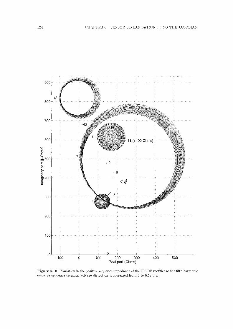
124 CHAPTER 6 TENSOR LINEARISATION USING THE JACOBIAN
900 ....
800
700
600
w .c: 0 d,500 t:: ell C.
c!' ell C: '6>400 ell E
300
200
100
13
· 1"1 ·(+)00-0htils} ·:- · · · · ·
/ 9
- 8 ························· . . . . . . . . . . . . . . . . . . . . . . . .
·<············••:••········
. . . . ·····-····························•.············••1•·············-·········· . . . . . . . . . . . . .
. . ···································•···················· ........................... .
0'------'~----'-------'-------'--'----'-------'----~---_,__ ___ _ -100 0 100 200 300 400 500
Real part (Ohms)
Figure 6.19 Variation in the positive sequence impedance of the CIGRE rectifier as the fifth harmonic negative sequence terminal voltage distortion is increased from Oto 0.12 p.u.

6.5 CONCLUSION
U) E .c 0
I =
800
600
~ 400 Cl.
2:(U C
-~ E
200
0
200A
• 2000A
3
:4
2000A
•. 2.
200A
200A
-200~~-----'-----'-------'---....L._--'--------'-----'------"'----100 0 100 200 300 400 500 600
Real part (Ohms)
125
Figure 6.20 Variation in the positive sequence impedance of the CIGRE rectifier as the current order is decreased from 2000A to 200A. Harmonics 2 to 6.

126
1600
1400
1200
E 1000 .c 0
I = t:'. ('O C.
~ 800 ('O C '0> ('O
E
600
400
200
0
CHAPTER 6 TENSOR LINEARISATION USING THE JACOBIAN
200 400 600 Real part (Ohms)
800 1000
Figure 6.21 Variation in the positive sequence impedance of the CIGRE rectifier as the current order is decreased from 2000A to 200A. Harmonic 7.

6.5 CONCLUSION
w E ..c
1800
1600
1400
0 ::!:,1200 t::: Cll 0.
C' Cll C ·a, Cll E - 1000
800
200A
200A:
.. 200A ..
1 2000A:
600
100 200
2000A
300 400 500 Real part (Ohms)
600
127
700 800
Figure 6.22 Variation in the positive sequence impedance of the CIGRE rectifier as the current. order is decreased from 2000A to 200A. Harmonics 8 to 12.

128
en E , .c 0
I = t
2000
1800
1600
cu 0..1400 ~ cu C ·oi cu E
CHAPTER 6 TENSOR LINEARISATION USING THE JACOBIAN
-200 -1 00 0 100 200 Real part (Ohms)
Figure 6.23 Variation in the positive sequence impedance of the CIGRE rectifier as the current order is decreased from 2000A to 200A. Harmonic 13.

6.5 CONCLUSION 129
alent impedances at the convertor bus. The impedances thus obtained were verified
against impedances calculated by a perturbation study at the convertor bus. A sparse
calculation of convertor impedances on the de side was implemented, and employed
the iterative refinement method. The de side impedances were verified against those
obtained from a frequency domain convertor model.
The convertor impedances were found to be affected by terminal voltage distor
tion. Characteristic harmonic impedances were found to be the most strongly phase
dependent, as predicted by a frequency domain convertor model. None of the convertor
impedances were magnitude dependent, indicating that the convertor is quite linear in
the harmonic domain. The convertor impedance was found to be a strong function of
the convertor operating point. A detailed study of this dependence would require more
genera.I modelling of a full de link.


Chapter 7
CONCLUSIONS AND FUTURE WORK
7.1 CONCLUSIONS
The proliferation of power electronic devices throughout the power system brings with
it a requirement for the modelling of these devices in the steady state, and the pro
pagation of the harmonic currents which they inject. Such an analysis is difficult, since
it involves both time and frequency dependent factors. Time domain analysis methods
have m'odelled the convertor well, but the ac system poorly. The reverse is true of
harmonic domain analysis methods. The primary objective of the research described
in this thesis was to develop a convertor model in the harmonic domain as accurate as
the time domain convertor model.
The first step in the development was to derive a new set of equations that fully
describe a twelve pulse controlled rectifier in the steady state. The equations developed
in Chapter 3 describe harmonic transfer through the 6-pulse bridge, and star-g/star or
star-g/delta connected transformers. The commutation process, and unbalance in the
convertor transformers have also been fully modelled. Interaction of the convertor with
circulating current in an unbalanced delta connection has been analysed for the first
time.
To solve the equations that describe the convertor, a set of mismatch equations
were constructed, suitable for solution by Newton's method. By utilising positive fre
quency harmonic phasors in the harmonic model, a decomposition to real components
in Chapter 4 permitted a fully unified solution of the harmonic interaction between the
ac and de systems, and the convertor switching instants. This is the first such unified
solution to be developed, and by introducing sparsity into the system Jacobian matrix,
the system of convertor equations was solved quickly.
The solution obtained was verified against time domain simulations of the rectifier
end of the CIGRE benchmark system. Rapid convergence was obtained even if a
composite ac/dc resonance was excited. Excellent correlation was obtained with time
domain simulations under a variety of severe unbalances. The model was also interfaced
to a three phase frequency dependent Thevenin equivalent of the New Zealand South
132 CHAPTER 7 CONCLUSIONS AND FUTURE WORK
Island system.
Alternative implementations of the convertor model in phase and sequence compo
nents were reported in Chapter 5. A polar components solution is impractica.! because
of poor conditioning, however a sequence components solution displays a much higher
degree of sparsity in the .Jacobian matrix. A decoupled solution, iterating between so
lutions of the ac/dc system harmonic interaction, and updates to the switching angles
was implemented. This method was found to diverge if even order harmonic sources
were present in the ac system.
The .Jacobian matrix employed in the Newton solution represents a linearisation of
all the equations that describe the convertor controller, harmonic interaction between
the ac and de systems, and the commutation process. A powerful and useful method
of extracting linearised relationships from the .Jacobian matrix was developed, and de
scribed in Chapter 6, with reference to the convertor harmonic impedance. Since the
convertor impedance is phase dependent, a more general representation of impedance,
the second rank tensor, was developed. Properties of the tensor, and a geometric inter
pretation of the tensor in the complex impedance plane was described. A nodal analysis
using a tensor admittance representation was then applied to the convertor, to derive
the convertor impedance at a particular harmonic and sequence. The impedance tensor
so obtained was verified against calculations of the convertor impedance obtained from
small harmonic perturbations. A sparse method for deriving linearised relationships
from large .Jacobians was also described, and then applied to the convertor model to
calculate the convertor de side impedance. The de side impedance was verified against
a frequency domain calculation of the impedance.
Finally, the effect of operating point and terminal voltage distortion on the con
vertor impedance was investigated. As expected, the convertor impedance was highly
dependent on operating conditions, however the tensor calculation of the impedance
developed in Chapter 6 provides a valuable tool for rapidly calculating the impedance
range.
7.2 FUTURE WORK
The research dPscribed in this thesis opens up many opportunities for future research
and development. LookiHg; first to the convertor model itself, improvements can be
made to both the degree, and extent of modelling. (:rea.ter gains however, would be
obtained from improving the extent of modelling as follows;
1. Transformer Connections The analysis of the convertor transformer should be
readily extendable to other transformer types, for example star/delta, star/star,
delta/star, and delta/delt,L Of a.II the transformer types, the star-g/dclta. is the

7.2 FUTURE WORK 133
only connection that converts some of the convertor positive and zero sequence
currents to zero sequence if the transformer is unbalanced,
2. Transformer Saturation Assuming that each convertor transformer consists
of three single phase units, accurate modelling of transformer core saturation re
quires just three additional variables in the Newton solution. These variables are
the direct currents shunted in the transformer secondaries. Three equations that
describe the de bias on the saturation curve would also be required. Harmonic
domain transformer models are well developed, and could be readily interfaced
to the convertor model. The magnetising currents in each phase, and their termi
nal voltage partial derivatives, would be calculated at each iteration by the time
stepping and FFT method.
3. Current Controller Any linear current controller could be modelled, since all
that is required is the appropriate transfer function from de ripple to alpha order
ripple. An arc-cos lineariser can be accurately modelled by linearising around the
average a.lpha order, on the assumption of a small alpha order ripple.
4. Inverter Control If the de source in the existing model is made negative, the so
lution obtained corresponds to a current controlled inverter. A minimum gamma
controller would require twelve additional equations, very similar to the end of
commutation mismatch equations, with roots at the negative going commutating
voltage zero crossings. From the twelve measured gamma, the minimum would
be selected at every iteration to be the control variable for the minimum gamma
mismatch equation: "fmin - "/order = 0.
5. Commutating Capacitance Extension of the commutation and de voltage sam
ple analyses to include series and shunt capacitance on the convertor transformer
secondary side, would be a valuable improvement to the model. This would allow
the modelling of series compensated convertor schemes, and the effects of stray
capacitance on de side harmonics as described by Shore et al. [1989]. It would
no longer be possible to refer thyristor resistance to the ac system, however the
average effect of thyristor resistance could be included as a constant voltage drop
on the de side.
6. Firing Error Firing errors can be specified in the model by adding a perturbation
to the equidistant timing references, for example setting f31 = 7r /6 + 6.01 would
introduce an error 6.01 to the first firing. Thus the maximum expected firing
error should be supplied to the model as well.
7. PLO The effect of terminal voltage harmonics on the phase locked oscillator, is
to introduce sampled error in the equidistant timing references. Frequently this
is the result of a process very similar to that of the firing pulse generator, but

134 CHAPTER 7 CONCLUSIONS AND FUTURE 'NORK
with a multiple cycle PI time constant. It should be possible therefore to combine
the two processes into one, by retaining perfect equidistant firing, but providing a
transfer function from sequence components terminal voltage harmonics, to firing
order ripple.
8. Link Control In the context of a unified harmonic domain model of a bipolar
link, several other controls must be modelled. These controls would each con
tribute one additional equation and unknown to the Newton solution, since tap
change control, reactive power compensation control, power control etc do not
respond to harmonics. Link controls have already been modelled in existing ac/dc
load flow programs.
9. Discontinuous Current If the de current is not continuous, additional equa
tions, similar to the end of commutation mismatches, are required. For each of
the twelve current pulses, an equation could readily be constructed that has a
zero at the end of the pulse. Applying the de voltage to the de system admit
tance, the resulting continuous current would be convolved with a 12 square pulse
sampling function to yield the discontinuous de current spectra.
The above points describe improvements that can be made to the extent of mod
elling of a single 12-pulse convertor. The methods employed to solve a single convertor
in this thesis, can clearly be used to model more of the power system as a whole. A
first step in this direction would be to augment the Jacobian matrix for the convertor
with the Jacobian matrix for a unified three phase load flow in rectangular coordinates.
A preliminary decoupled ac/dc load flow and harmonic convertor solution diverged
due to interaction between unbalance in the ac system, and triplen harmonic injection
from the convertor. A unified solution is therefore recommended, both to improve
convergence, and to match the convergence rate between the load flow and convertor
model. Although the fast decoupled ac/dc load flow has been found to be very efficient,
the large number of iterations required to converge should be avoided if the harmonic
model of the convertor is included. This is because the convertor model is more difficult
than the load flow, and typically converges in only seven iterations.
The following implementation of a unified load flow and harmonic convertor model
is suggested:
• Perform an initial ac/ de load flow, with no harmonics, and utilising the switching
system convertor model.
• Calculate a unified load flow and harmonic convertor model Jacobian matrix.
• Solve the load flow and convertor model with constant, but sparse Jacobian.

7.2 FUTURE WORI< 135
• Recalculate the full Jacobian at the solution, and calculate any linearised rela
tionships required.
The Jacobian for the unified solution consists of the Jacobians for the load flow
and convertor arrayed on the main diagonal, and twelve cross coupling terms for each
ac system bus to which the convertor is directly attached.
At some point it will be necessary to extend the convertor model to encompass
a full bipolar de link. In general, the de current in the two poles will be different,
implying 800 harmonic unknowns, 96 switching instants, and several control variables.
The structure of the Jacobian however, would be very similar to that developed for the
single twelve pulse convertor, and the solution time will scale linearly with the size of the
problem. In order to increase availability, de links have many operating configurations
corresponding to different combinations of six pulse groups being blocked. It would
therefore be desirable to develop a de link model that mirrored a similar modular
structure so that it could solve each of these configurations.
If the de link is between two separate ac systems, solutions can be obtained for a
variety of phase angles by adding an offset to the angle of the internal emf of the slack
bus generator in one of the ac systems. This approach is based on the assumption
that the two ac systems are bound to be of very similar frequency, perhaps differing by
0.lHz. A de link between systems at 50Hz and 60Hz would require that the fundamental
frequency of the model be set to lOHz, with the primary excitation in the two systems
being at the 5th and 6th harmonics respectively. This requires that 5.5 times as many
switching angles be solved as well, however once again, the structure of the Jacobian
is quite similar to that developed in this thesis.
Eventually it would be desirable to develop a general purpose model with facility
for several ac systems, de systems, and possibly with multiple terminals in each system.
This is essentially a software engineering task, as each half pole contributes a block to
the main diagonal of the system Jacobian matrix, with diagonal matrices coupling to
other harmonic sources in the same system. The main task is to code the program so
as to be versatile, easy to use, and modular.
Continuing with this theme, the methods of analysis employed in this thesis to anal
yse the convertor, are also applicable to FACT devices. It particular, the TCR should
be the next device to be modelled in the harmonic domain, since it has similarities with
the commutation analysis for the convertor.
The convertor model is at a stage where it could be integrated with the existing
Harmonic Domain Analysis (HDA) program by modifying the phase components lattice
tensor to a complex conjugate harmonic admittance matrix. By solving the interaction
with the de system at each iteration, the convertor model could be used to construct
a Norton equivalent for the convertor. However this is less efficient than a full Newton
solution.

136 CHAPTER 7 CONCLUSIONS AND FUTURE WORK
Although the range of devices that can be modelled in the harmonic domain has
been extended in this thesis, there is no reason to believe that every device that we may
wish to model will fall neatly into a set of harmonic domain equations. An example
is transformer saturation, for which the time stepping and FFT method is both fast
and simple. In proposing a structure for the general modelling of the ac system in
the steady state, it is therefore necessary to be as general as possible, and to place no
constraints on future models.
As discussed in Chapter 2, there has been an over emphasis on the use of elec
trical equivalents in the complex conjugate space. This restricts the solution method
employed, since it is not possible to include real valued, non-electrical quantities in
the solution. Some authors have therefore iterated between an electrical equivalent of
the system, and separate procedures, possibly Newton, to solve for the other variables.
This type of iteration is inefficient, and displays poor convergence. The overall ap
proach of a Newton solution in real variables, is quite general. As discussed above, the
load flow is readily integrated with equations for switching instants, control variables,
and harmonic interactions.
The Newton solution method in real variables, is also compatible with any type
of device model. For example, a time stepping model of the convertor, with specified
terminal voltage, de current harmonics, and switching angles, could be used to calculate
all of the convertor mismatches instead of the harmonic phasor equations used here.
Although the Jacobian matrix would be kept the same, the time stepping model could
include snubbers, and the conduction characteristic of the thyristors. Although it is
not suggested that such a model be developed, it is clearly possible to interface FAST
solutions of difficult nonlinearities via a voltage or current mismatch to the overall
Newton solution. The required partial derivatives could be obtained from a less general
harmonic domain model, or a perturbation method.
A unified load flow and harmonic domain convertor model could therefore provide
the core for a general purpose power system steady state solution. Nonlinear device
models would be developed separately with a Thevenin equivalent of the ac system, and
then interfaced to the system model as a block diagonal in the system Jacobian. The
nonlinear device models could be achieved by means of harmonic domain equations,
modulation theory analysis, or time domain simulation.
By careful attention to sparsity and efficiency, a general power system steady state
solution would be fast, and would scale linearly. Rapid steady state solutions to the
power system would provide a basis for stochastic harmonic modelling, previously too
difficult. The reliability analysis of' the power system at fundamental frequency is now
well established, and employs a load flow as the system solution. Reliability analysis
has also been applied to the IIVdc link, and an interesting possibility for future research
would be to integra.te a reliability analysis of the power system with a. three phase loa.d

7.2 FUTURE WORI< 137
flow and harmonic solution of the power system. The present convertor model converges
in approximately three seconds for multiple solutions on a Sun Sparcstation V. It would
therefore be possible to enumerate a de link model, with load flow, over several thousand
operating conditions and contingencies. The outcome of the enumerated solution would
be a probability density function for every harmonic and sequence, at every bus in the
power system.
Such a stochastic harmonic system model is the proper framework within which
to account for variabilty in the system impedance, random firing errors, background
harmonic sources, and highly variable harmonic injections such as the arc furnace. It
would therefore provide a valuable tool for assessing the overall harmonic performance
of a power system.
Having converged to the system solution, the sparse calculation of impedances from
the system Jacobian developed in Chapter 6 becomes a very powerful tool. Any linear
relationship between system variables can be extracted from the Jacobian. Examples
are harmonic transfers through a back to back de link, harmonic influence factors, har
monic currents shunted in a filter bank due to another electrically close injection source,
voltage stability factors, firing angle modulation transfers etc. Harmonic impedance
calculations at nonharmonic frequencies could be obtained by calculating a larger in
terharmonic Jacobian, for a system with a l0Hz fundamental for example. However a
more promising approach is to apply a modulation analysis to the sampling functions
calculated at the system harmonic solution.
Of great interest would be the investigation of a phase dependent resonance or
harmonic magnification factor, at either the 5th or 7th harmonic, for a twelve pulse
convertor.
Apart from research and development directed at enhancing the extent of har
monic modelling, several improvements to the numerical solution of the convertor model
should make it considerably faster:
• The initial calculation of the sparse Jacobian is quite slow. Approximately 40%
of the total solution time is spent calculating and scanning the full Jacobian in
a checkerboard pattern to locate significant elements. This process could almost
be eliminated by scanning only the three port terms, and rows associated with a
resonance in the ac or de systems.
• A hybrid use of voltage or current mismatches, depending upon the ac or de sys
tem impedances, should lead to a more robust solution. In this method, a voltage
mismatch would be used if the system impedance was less than 1 p. u., otherwise a
current mismatch would be used. This ensures that the system impedance or ad
mittance is never greater than 1 p.u., a definite possibility if the group connection
is to be modelled, or if there are no filters.

138 CHAPTER 7 CONCLUSIONS AND FUTURE WORE
• The decoupled method was found to diverge if even order harmonic sources are
present in the ac system. A Kron reduction of the full Jacobian to the ac/dc and
switching system Jacobians, should improve the convergence of the decoupled
method. Use of the Kron reduction in this manner means that a linearised rep
resentation of the ac/dc harmonic interaction is present in the switching system,
and vice versa.
• A possibility for future research is to decouple the harmonic analysis of the power
system into a set of three harmonic interactions; harmonics k + 1 and k - 1, in
positive and negative sequence respectively, in the ac system, and harmonic k
in the de system or machine rotors. This decoupling could form the basis of a
parallel system solution.

Appendix A
HARMONIC PHASORS
This appendix provides basic background theory on Fourier analysis, harmonic phasors,
and discrete convolutions. The phasor representation of a sinusoidally varying quantity
is widely used in power systems analysis for undistorted waveforms. Representation of
the phasor has been by means of polar co-ordinates ( as in the decoupled load flow), or
complex rectangular co-ordinates. The complex rectangular representation allows easy
addition and multiplication of phasors, and reactive components are easily modelled
by an imaginary impedance.
The representation of non-sinusoidal periodic waveforms has commonly used the
complex Fourier expansion. The terms in this expansion however, are not complex
harmonic phasors. They are complex conjugate pairs associated with the positive and
negative harmonic components of the expansion. The complex Fourier series has been
used because of its compatibility with the Fast Fourier Transform, a central component
of the hybrid time stepping and harmonic injection method of analysis. A useful feature
of the complex conjugate representation is that it allows the modelling of the phase
reversal of some devices by inclusion of a coupling admittance between the positive and
negative frequencies.
If frequent transforms into the time domain are not required, a harmonic phasor
Fourier expansion offers several advantages; the redundancy of storing and processing
complex conjugate pairs is avoided, the harmonic phasor is compatible with existing
analysis methods ( such as the load flow), and it is easy to decompose the phasor
into real components affording compatibility with the large body of numerical solution
packages available on the Internet. Finally, the decomposition into real cornpo11c11t.s
is necessary in this thesis in order to develop a unified solution of harmonic phasors,
which are complex, and switching angleci, which are real.

140 APPENDIX A HARMONIC PHASORS
A.1 THE FOURIER SERIES IN PHASOR FORM
Fourier Theory states that a periodic and integrable function can be represented by an
infinite series of trigonometric functions:
co Clo ~ J (t) = 2 + D [ak cos kwt + bk sin kwt],
k=l
(A.l)
where
1 !Jr Clk ; -1r J(wt)cos(kwt)d(wt)
1 !Jr bk = ; -1r J(wt)sin(kwt)cl(wt). (A.2)
This theory forms the basis of harmonic domain analysis. The fundamental frequency,
w, is chosen to correspond to the duration of one cycle of the periodic steady state,
usually 50 or 60 Hz. In the case of a back to back link connecting 50/60 Hz systems, a
frequency of 10 Hz would be appropriate in order to resolve all the relevant frequencies.
A frequency of 1 Hz could be used to analyse subsynchronous and interharmonic phe
nomena, while 0.1 Hz resolution could be suitable for analysing transient phenomena.
The trigonometric Fourier expansion A.l can be converted into a complex expo
nential Fourier expansion by substituting the following identities for the trigonometric
terms:
sin (kwt) 2j
cos (kwt) ejkwt + e-jkwt
2 (A.3)
This results in:
co
f (t) = L Ckejkwt, (A.4) -co
where
(A.5)
The complex Fourier series expansion is compatible with the Fast Fourier Trans
form, the method of choice for converting; time domain da.ta samples into a. Nyquist rate
limited frequency spectrum. The trigonometric Fourier expansion can also be written
A.2 CONVOLUTION OF HARMONIC PHASORS
as a series of phase shifted sine terms by substituting
ak cos kwt + bk sin kwt = rlic sin (kwt + 7/Jk)
into equation A.l, where
-1 Clk tan -b .
k
141
(A.6)
(A.7)
Finally, the phase shifted sine terms can be represented as peak value phasors by setting
(A.8)
so that
ch sin (kwt + 1Pk) I{Wkejkwt}
l'11kl sin (kwt + L'.'.\llk), (A.9)
The harmonic phasor Fourier series is therefore:
00
f(t) = LI{Wkejkwt}, (A.10) k=O
which does not contain negative frequency components. Note that the de term becomes
Clo . rr -elz 2 .(lo J-
2 (A.11)
In practice, the upper limit of the summation is set to nh, the highest harmonic order
of interest. The use of peak value phasors means that the complex power is given by;
P+jQ=lvr, (A.12)
where V and I are peak values at the fundamental.
A.2 CONVOLUTION OF HARMONIC PHASORS
The point by point multiplication of two time domain waveforms is expressed in the
harmonic domain by a discrete convolution of their Fourier series. When two harmonic
phasors of different frequencies are convolved the result are harmonic phasors at sum
and difference harmonics. This is best explained by multiplying the corresponding
sinusoids using the trigonometric identity for the product of sine waves, and then

142 APPENDIX A HARi'vIONIC PHASORS
converting back to phasor form. Given two phasors, Ak and Bm, of harmonic orders k
and m, the trigonometric identity for their time domain multiplication is:
I Aki sin (kwt + L'.'.Ai,,) IBm I sin (mwt + LBm) =
}IAkllBml [sin ( (k - ni)wt + LAk - LBm + i) - sin ((k + m)wt + L'.'.Ak + LBm + %) ] .
Converting to phasor form:
!IAkllBml [ej(LAk-LBm+})I - ej(LAdLBm+})I ] 2 (k-m) (k+m)
(A.13)
} [(IAklejLAklBmle-jLBmeJf)k_m - (IAklejLAklBmlejLBmeJf)k+m]
}j [(AkB::ih-m - (AkBmh+m] (A.14)
If k is less than m, a negative harmonic can be avoided by conjugating the difference
term. This leads to the overall equation:
(A.15)
The multiplication of two nonsinusoiclal periodic waveforms leads to a discrete convo
lution of their harmonic phasor Fourier series:
nh nh
fa(t)fb(t) = L !Aki sin (kwt + LAk) L IBkl sin (mwt + L'.'.Bm) k=O m=O nh nh
LL IAkl sin (kwt + LAk)IBkl sin (mwt + L'.'.Bm), (A.16) k=O m=O
Rewriting this in terms of phasors yields
nh nh
FA 0 FB =LL Ak @Bm, (A.17) k=Om=O
Equation A.17 generates harmonic phasors of order up to 2nh, clue to the sum terms.
Substituting the equation for the convolution of two phasors, equation A.15, into A.17,
and solving for the Ith order component yields:
(A.18)
A.2 CONVOLUTIO:\' OF HARMO>iIC PHASORS 143
(A.19)
The convolution equations a.re non-analytic in the complex plane, but are differentiable
by decomposing into two real valued components (typically polar or rectangular).


Appendix B
TEST SYSTEMS
B.1 CIGRE BENCHMARK
The test systems used in this thesis are based on the rectifier end of the CIGRE
benchmark model [Szechtman et al. 1991]. The inverter side has been replaced by
a constant de voltage source, E, as illustrated in figure B.1. The benchmark model
0.5968 2.5 2.5 0.5968
Tss
t + 26.0
E
t •1~685
83.32
Figure B.1 Rectifier end of the CIGRE benchmark model. Components values in n, H, and µF.
consists of a weak ac system, parallel resonant at the second harmonic, coupled via the
rectifier to a de system that is series resonant at the fundamental frequency. These
features are shown in the impedance plots of figures B.2 and B.3. The system therefore
displays a composite resonance between the ac and de systems. The ac system is
balanced, and is connected in grounded star, as are both converter transformers on the
ac side. Additional parameters for the system are listed in table B. l.
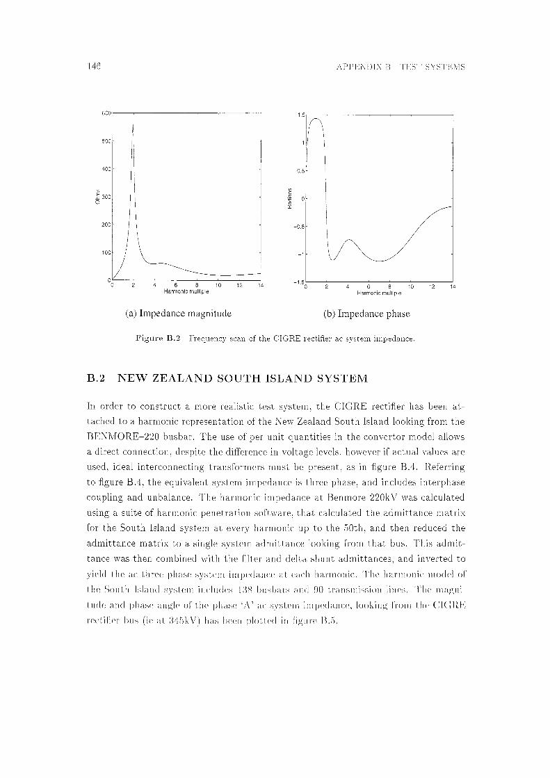
146
600,---,-----,------------,
500 '-
400
~ 300 0
200
100
o~-~-~-~~-~-~-~
0 2 4 6 8 10 12 14 Harmonic multiple
(a) Impedance magnitude
APPEKDIX B TEST SYSTEMS
1.5-------------~
{\ I
0.5
-0.5
-1
-1.s~~-~-~-~-~-~-~ 0 2 4 6 8 10 12 14
Harmonic multiple
(b) Impedance phase
Figure B.2 Frequency scan of the CIGRE rectifier ac system impedance,
B.2 NEW ZEALAND SOUTH ISLAND SYSTEM
In order to construct a more realistic test system, the CIGRE rectifier has been at
tached to a harmonic representation of the :\ ew Zealand South Island looking from the
BE>lrvIORE-220 busbar. The use of per unit quantities in the convertor model allows
a direct connection, despite the difference in voltage levels. however if actua.l va.lues are
used, ideal interconnecting transformers must be present, as in figure B.4. Referring
to figure BA the equivalent system impedance is three phase, and includes interphase
coupling and unbalance. The harmonic impedance at Benmore 220kV was calculated
using a suite of harmonic penetration software, that calculated the admittance matrix
for the South Island system at every harmonic up to the 50th, and then reduced the
admittance matrix to a single system admittance looking from that bus. This admit
tance was then combined with the filter and delta shunt admittances, and inverted to
yield the ac three phase system impedance at each harmonic. The harmonic model of
the South Island system includes 1:rn busbars and 90 transmission lines. The magni
tude and phase angle of the pha.se 'A' ac systern impedance, looking from the CIGRE
rectifier bus (ie at 345kV) has been plotted in figure B.5.

B.2 NEW ZEALAND SOUTH ISLAND SYSTE?vI 147
6000--~-~----~---~
5000
4000
(/)
_g 3000 0
2000
1000
0.5
(/)
-~ 0
£ -0.5
-1
-1.5
2 4 6 8 Harmonic mulllple
10 12 -2'---~-~-~--~-~-~
0 2 4 6 8 10 12 Harmonic multiple
,(a) Impedance magnitude (b) Impedance phase
Figure B.3 Frequency scan of the CIGRE rectifier de system impedance.
power base 603.73 MVA primary voltage base 345 kV secondary voltage base 213.4557 kV nominal de current 2000 A nominal firing angle 15° de voltage source 4.179 p.u. transformer leakage reactance 0.18 p.u. transformer series resistance 0.01 p.u. thyristor forward voltage drop 8.llE-6 p.u. thyristor on resistance 0.001325 p.u. de current transducer time constant 0.001 s/rad PI controller proportional gain 1.0989 rad/ A(p.u.) PI controller time constant 0.0091 s/rad
Table B.1 Parameters for the CIGRE benchmark rectifier.

148
exact equivalent harmonic 3 phase impedance i ~ •/~ Yth
------------
BENMORE--220
/ 220:345, ideal
•1~29.76 0.1364 6-685
74.28 261.87
-,~"' 83.32
APPENDIX B TEST SYSTEMS
, , , , , ' ' CIGRE rectifier
0.5968 2.5 2.5
26.0
0.5968
+
E
Figm•e B.4 Rectifier end of the CIGRE benchmark model attached to New Zealand South Island system. Components values in 0, H, and µF.
New Zealand SI system impedance at BENMORE--220 80 I I I I ' I I I I
...
~
~ - -- - -
0 ~~1 UIIII 5 10 15 20 25 30 35 40 45 50
Harmonic Order
,5 10 15 20 25 30 35 40 45 50 Harmonic Order
Figure B.5 Phase 'A' of the calculated New Zealand South Island system impedance looking from the CIGRE rectifier bus, under conditions of 100% load and generation.
Appendix C
DERIVATION OF THE JACOBIAN
In this appendix, the full Jacobian matrix is derived for a six pulse rectifier attached to
the ac system via a star-g/star transformer. The elements of the Jacobian are the partial
derivatives of the mismatch functions with respect to the variables that are being solved
for by Newton's method. An important distinction is made in Newtons method between
functions and variables. A variable is never a function of something else. A function is
only a function of the variables being solved for, and never another mismatch function.
The variables that are being solved for are defined to be Vt, Vf, Vk, Idk, </>i, 0i, o:0 . Thus
Idk, the de current harmonics, are defined not to be a function of Vk, the terminal
voltage harmonics. In the analysis to follow, any other quantity is either a function of
these variables or a constant.
In finding the partial derivative of a mismatch function with respect to one of these
variables, all other variables are held constant. Thus the chain rule is never applied
to give a derivative of one variable with respect to another. For example, in the de
current mismatch equations, the partial derivative with respect to the average delay
angle is always zero. Intuitively this is ·incorrect, as we expect a change in delay angle to
change all the de harmonics. However, in terms of the convertor mismatch equations,
this requires several applications of the chain rule to quantities that have been defined
as variables, not functions. The overall network of interdependency between all the
convertor quantities is only fully represented in the inversion of the Jacobian matrix,
and in the definition of the mismatch functions.
All of the partial derivatives obtained below have been confirmed by comparison
with the numerical partial derivative obtained from the corresponding mismatch equa
tion. That is;
{)F F(x + 6.x) - F(x) -~--------{)x 6.x
(C.l)

150 APPENDIX C DERIVATION OF THE JACOBIAN
C.1 VOLTAGE MISMATCH PARTIAL DERIVATIVES
The voltage mismatch partial derivatives are obtained by first deriving the phase cur
rent partia.l derivatives, and then applying the differential current to the three phase
system impedance. The phase current partial derivatives are derived in turn by con
sidering the partial derivatives of the sampled commutation and de currents of which
they are composed.
C.1.1 With Respect to Ac Phase Voltage Variation
First, the partial derivative of the terminal voltage mismatch ,vith respect to terminal
voltage variation is obtained. In this analysis all other variables are held constant.
The commutation current, sampled de current, and phase currents are all functions,
and require an application of the chain rule. The phase voltage mismatch equation,
which represents the interaction of the calculated phase currents with the ac system
impedance is
Fvt = Vt - [ z,ra ( If + [½ci1th]n + z;!3 (If + [Ytc vth]f) + z;, (Il + [Ytc vth]k}] (C.2)
In order to generalise over all phases, [n (3 1] is a permutation of [a b c]. Z = Yc;:- 1 is the ac system impedance, and Ia etc are the phase currents. Note that
I (Vt, Vf, V{, Idk, <Pi, 0i) is a function of the convertor variables. Since the terminal
voltages are represented as complex phasors, it is necessary to differentiate with re
spect to the real and imaginary parts separately. Differentiating equation C.2 partially
with respect to a variation in one of the phase voltages:
EJR{Fvt} _ { EJR{VJi} - R
n /. 8 or k-/- m
' n = 8 and k = {t.3)
(C.4)
n /. 8 or k f:. ,n )
n = 8 and k = n(C.5)

C.l VOLTAGE MISMATCH PARTIAL DERIVATIVES 151
8I{Fvt} { zcw &If o:/3 8If o:-r 8IJ } 8R{V~} = I - k 8R{V~} - z,., 8R{VJi} - z,., 8R{VJi} '
(C.6)
Since the ac phase currents are calculated by sampling the de and commutation
currents, the effect of phase voltage variation on phase current is determined from the
effect of phase voltage variation on the sampled commutation currents alone. This is
because the de current and switching angles are variables which are held constant, while
the commutation currents are functions of the terminal voltage. Four commutations
contribute to one cycle of ac current, consequently
8/k ~ 8fci 8R{V0 } = ~ Co:o; 8R{V0}'
m i=l m
(C.7)
and
8/0: 6 8/8, k """c c,k
-8I-{V.~0-} = ~ o:c5; 8I{V.0 } ' m i=l m
(C.8)
where 1:i is the ith commutation current, lei, sampled over the commutation period.
Co:o; €. [-1, 0, 1] is a coefficient matrix that defines whether for the ith commutation the
phase a current is a function of the phase (3 terminal voltage, and if so, in which sense.
C is defined in the following table where i indexes each set of data: The commutation
8 a b C
a {-1, o, -1, -1, o, -1} {0,0,1,0,0,l} {1,0,0,1,0,0} a b {o,o,1,0,o,1} {O, -1, -1, O, -1, -1} {0,1,0,0,1,0}
C {1,0,0,1,0,0} {0,1,0,0,1,0} {-1, -1, O, -1, -1, O}
Table C.1 The coefficient matrix Oa6; which specifies the dependence between commutation current i, terminal voltage phase, and ac current phase.
current is given by
where
nh
lci(t) = D + L fcikejkwt, k=l
nh
D = -I{LlcikejkO;},
k=l
(C.9)
(C.10)

152 APPENDIX C DERIVATION OF THE JACOBIAN
I . - jkwLJdk - \lebk c,k - jkwLeb (C.11)
In equation C.11, e and b a.re subscript functions of i, and refer to the phases ending
and beginning conduction respectively. Sampling the commutation current requires a.
convolution with the relevant sampling function:
(C.12)
Setting Icio = D, expanding the convolution, and ta.king the kth component yields
Since the commutation circuit is linear,
8Ici1 BR{VJJ = 0 \;/ l, m such that l i= m and l > 0.
This allows the following partial derivative to be written:
+{ EJici W - EJR{V".!,} (2i-l)k_m'
EJicim '1J* EJR{Vi,} (2i-l)m-k'
Similarly,
EJicim W - EJT{Vi,} (2i-l)k_m'
EJ lei W* EJT{vl} (2i-l)m-k'
m>k
m~kl· m?. k
(C.14)
(C.15)
The calculations required to evaluate equations C.14 and C.15 can be approxi
mately halved by using the Cauchy Reimann equations for the partial derivatives of
complex functions. For an analytic function
8F(z) . 8F(z) 8I{z} = J 8R{z}'
(C.16)

C.l VOLTAGE MISMATCH PARTIAL DERIVATIVES 1.53
For the complex conjugate of an analytic function
8F(zf . fJF(z)" oI { z} = - 1 an { z} · (C.17)
Thus, as each term of equation C.14 is evaluated, the corresponding term in equa
tion C.15 is obtained from a simple rearrangement of the real and imaginary parts. The · ' t' 1 d ' t' Bicio d Bicim bt · d f · C 10 remamrng par 1a enva 1ves, EJR{VJi} an EJR{Vi,}, are o a.me rom equat10ns .
and C.11;
(C.18)
Olcio ·n { ejke; } -8I_{_V_~_} = -J jkwLeb ' (C.19)
Ofcim l fJR{V~} - jkwLeb.
(C.20)
It is assumed here that phase 8 is beginning conduction; phase 8 ending conduction
is accounted for in the C matrix. This completes the derivation of the partial derivative
of terminal voltage mismatch with respect to terminal voltage.
C.1.2 With Respect to De Ripple Current Variation
A variation in the de ripple at a particular harmonic is sampled by the compound de
current sampling function, and so affects all phase current harmonics. In addition, the
commutation currents are functions of the de ripple, and so the resulting variation in
commutation currents are sampled on the ac side by the commutation interval sampling
functions. These two effects, when added together, are sufficient to give the variation
in phase currents, and by injecting the phase current variation into the ac system, the
required mismatch partial derivative for the Jacobian matrix is obtained. The voltage
mismatch partial derivatives are therefore
(C.21)
(C.22)

154 APPENDIX C DERIVATION OF THE JACOBIAN
(C.23)
(C.24)
The phase currents are composed of commutation currents and the de current sampled
on the ac side:
6
l 0 = L [E.; lei® W2i-1] +Id® Wa. i=l
(C.25)
Here E'f is a coefficient matrix that specifies how the commutation currents contribute
to each of the phase currents, and '1! 0 is the phase a de current compound sampling
function. E is listed in table C.2 Differentiating the kth component of equation C.25
a a b C
1 1 0 -1 2 0 -1 1
i 3 -1 1 0 4 1 0 -1 5 0 -1 1 6 -1 1 0
Table C.2 Coefficient matrix Er defining the contribution of the commutation currents to each phase current. i is the commutation number.
with respect to 1l{Idm} yields
(C.26)
The first term is similar to the differential with respect to voltage already derived
above, as a variation in Idm affects only Icim and Icio. Expanding the convolution in
the first term, selecting the kth component, and differentiating yields
m~kl m '?:. k
. (C.27)

C.l VOLTAGE MISMATCH PARTIAL DERIVATIVES 155
Expanding the convolution in the second term of equation C.26 gives the kth component
of the sampled de current:
where IJ; is the phase O' sample of the de current. This equation can be differentiated
to yield:
(C.29)
Applying the above analysis for variations in the imaginary part of Idm gives
(C.30)
and
(C.31)
These equations are then substituted into an equation analogous to equation C.26 and Eilcio d hence into equations C.22 and C.24. The remaining partial derivatives, DR{Idm} an
a~h;,:,}, are obtained from equations C.10 and C.11:
(C.32)
(C.33)
{)fcim Le 8R{Idm} Leb
(C.34)
156 APPENDIX C DERIVATION OF THE JACOBIAN
C.1.3 With Respect to End of Commutation Variation
A variation in the end of commutation angle, rl>h, affects the (2h - l)th and 2hth
sampling functions. This affects all harmonics of the ac side sampled commutation
currents, and de current. Combining these two effects into the phase current variation,
and injecting into the ac system yields the variation in the terminal voltage mismatch;
(C.3.5)
(C.36)
Differentiating the kth component of equation C.2.5 with respect to <Ph,
(C.37)
A variation in ¢h affects only the sampling of the hth commutation current in the first
term of equation C.37. Expanding only this convolution from the summation yields
Differentiating this gives
(C.39)
where
(C.40)
The compound sampling function in the second term of equation C.37 is affected
by variation in four of the six end of commutation angles. This is because the transfer
of de current to the ac side is defined by two conduction periods per cycle; the be
ginning and end of each conduction period corresponding to an end of commutation
angle. The effect of a variation in <Ph therefore depends upon whether it corresponds

C.l VOLTAGE MISMATCH PARTIAL DERIVATIVES 157
to the beginning or end of a positive or negative conduction period for phase a. This
information is already collated as the coefficient matrix -E0 ,.
A similar analysis to the above for the second term of equation C.37 results in
(C.41)
Since the compound sampling function is a sum of constituent sampling functions, it
has been replaced in the partial derivative by the only term which is a function of </>h. This is then substituted back into equation C.37 to give the required partial derivative.
C.1.4 With Respect to Firing Angle Variation
The transfer of de current to the ac side of the convertor is defined entirely with
reference to the end of commutation angles. The effect of a variation in the firing
instants on the phase currents can therefore be obtained by analysing just the sampling
of the commutation currents. The partial derivative of the ac voltage mismatch with
respect to a firing angle variation is
8R{ Fv;:} = R {-zoo 8If _ zo:.G 8If _ zo:"f 8IJ} ,:i0 k ,:i0 k ,:i0 k ,:i0 , uh uh uh uh
(C.42)
Since the ac side sampled de current is not a function of 01i
a { Lf=1 Ef 1:i t {) { Lf=l Ef lei Q9 W (2i-1)} k
80h
8 {E'f:lch ® W(2h-1)}k
80h 801i (C.43)

158 APPENDIX C DERIVATION OF THE JACOBIAN
Noting that a change in 0h affects Icho and \JJ( 2h-l), applying the product rule to the
expansion of the convolution leads to
(C.44)
This completes the analysis of the terminal voltage mismatch equation partial deriva
tives, as there is no dependence upon Go, the only remaining variable.
C.2 DIRECT CURRENT PARTIAL DERIVATIVES
The direct current partial derivatives are obtained by a process analogous to that used
in obtaining the terminal voltage partial derivatives. The de voltage partial derivatives
are obtained and then applied to the de system admittance to calculate the direct
current differential. The direct current mismatch equation is:
(C.45)
Finding the partial derivatives of this equation is therefore mainly concerned with Vdk,
which is a function of all the convertor variables except 0'0 •
C.2.1 With Respect to Ac Phase Voltage Variation
Differentiating equation C.45 with respect to terminal voltage yields
(C.46)
(C.47)
(C.48)
(C.49)

C.2 DIRECT CURRENT PARTIAL DERIVATIVES 159
Vak is given by:
The only terms in this equation which are a function of V~ are the twelve pre-convolved
de voltage phasors Vai1• There are three equations which define the twelve pre-convolved
de voltage phasors;
(C.51)
for a 'normal' conduction interval,
(C.52)
for a commutation on the positive de rail, and
(C.53)
for a commutation on the negative rail. Differentiating these three equations with
respect to V~ gives 36 possible values for ~~~1 according to the sample number -i, m
and the phase of fJ, The required partial derivatives are summarised in table C.3 by
reference to the partial derivatives of equations C.51, C.52, and C.53 listed below:
8Vai1 an{v/} = 1
avai, = _1 an{l't-}
for a 'normal' conduction interval,
8Vai1 Lb o'R{l'te} Lb+ Le
avai1 Le an{vl} Lb +Le
avai1 -1 8'R{'\1io}
(C.54)
(C.55)

160 APPENDIX C DERIVATION OF THE JACOBIAN
for a commutation on the positive de rail, and
avdii Lb 8R{l1ie} Lb+ Le
avdii Le 8R{l7ib} Lb+Le
avdi, 1
8R{l1i0 }
(C.56)
for a commutation on the negative rail. The Cauchy Reimann equations can be used to
give the partial derivative with respect to the imaginary part of the voltage variation
as j times that listed above.
sample (i) De Voltage derivative e b 0 + - eqn
1 A C B (C.55) 2 A B (C.54) 3 C B A (C.56) 4 A C (C.54) 5 B A C (C.55) 6 B C (C.54) 7 A C B (C.56) 8 B A (C.54) 9 C B A (C.55) 10 C A (C.54) 11 B A C (C.56) 12 C B (C.54)
Table C.3 Assembly of de voltage partial derivatives
The partial derivatives in equations C.54, C.55, and C.56 are then substituted into
the partial derivatives of equation C.50 which are given below:
(C.57)

C.2 DIRECT CURRENT PARTIAL DERIVATIVES 161
(C.58)
This completes the derivation of the partial derivative of de current mismatch equation
with respect to terminal voltage.
C.2.2 With Respect to Direct Current Ripple Variation
Apart from being the most significant term in the de current mismatch equation, the
de ripple affects the commutation currents, and also causes a voltage drop through the
commutating reactance. These last two effects mean that the de voltage is a function
of the de current ripple. It is therefore necessary to obtain partial derivatives of the
de voltage harmonics in a similar manner to that undertaken already for the derivative
with respect to terminal voltage. Differentiating the de current mismatch equation;
k =/:- rn k = rn
Differentiating equation C.50 with respect to R.{ Idm} yields
rn~kl rn ?:. k
, lexk > 0.
(C.59)
(C.60)
(C.61)
(C.62)
(C.63)
162 APPENDIX C DERIVATION OF THE JACOBIAN
Similarly,
- , lexk > 0. m <kl m?:. k
(C.64)
Tl t . 1 d · · avdim bt · d f t' C 51 C 52 d C' -3 1e par ia envat1ves BI{Idm} are o arne ram equa ions . , . , an ,.b :
(C.65)
during normal conduction, and
oVdim _ 'k [L LeLb ] oR{I } - J w O + L + L dm e b
(C.66)
during any commutation. Again, the imaginary partial derivatives are obtained by
the Cauchy Reimann equations. The correct phase subscripts can be obtained from
table C.3. This completes the linearised dependence of the de mismatch upon de ripple
variation.
C.2.3 With Respect to End of Commutation Variation
The effect of variation in the end of commutation angle cf>h is limited solely to the
sampling of relevant de voltage sections. This is best explained with reference to the
following equation for the de voltage:
1 12
Vi= 2J L Vii® wi. i=l
(C.67)
In this equation, only two of the twelve Wi are functions of o/h· Table C.4 shows that
W2h and W2h-1 are functions of (Ph. Equation C.50 can therefore be differentiated to
yield:
(C.68)

C.2 DIRECT CURRE:\"T PARTIAL DERIVATIVES 163
sample (i) Cli bi 1 01 ¢1 2 ¢1 02 3 02 ¢2 4 ¢2 83 5 03 ¢3 6 ¢3 04 7 04 ¢4 8 ¢4 05 9 05 ¢5 10 ¢5 06
11 ()6 <P6 12 <P6 01
Table C.4 Limits of convertor states for use in sarnpli?-g functions
Differentiating the de ripple mismatch equation C.45 yields:
(C.69)
and
(C.70)
Substituting equation C.68 into C.69 and C.70 gives the required partial derivative of
de ripple mismatch with respect to end of commutation.
C.2.4 With Respect to Firing angle variation
The partial derivatives of de ripple mismatch with respect to firing angle are obtained
in an exactly similar manner. The result is:
(C.71)
and
(C.72)

164 APPENDIX C DERIVATION OF THE JACOBIAN
where
fJVik a01i
1 . / a\J!21ik-l I a\J!2h1-k * (
k nh
2J ~ 1 d(2h-2)1 aeh - ~ 1 d(2h-2)1 ( fJ01i )
nh [ 0ffr ] * k {)ff• I U'i'2h-11-k * I 'i'2h-lk-l - L 1 d(2h-2)1 ( {)0 ) ) - L 1 d(2h-1)1 80 l=O h l=O h
C.3 END OF COMMUTATION MISMATCH PARTIAL DERIVATIVES
(C.73)
The end of commutation mismatch is the current in the phase that is commutating off,
at the end of the commutation. This current should be zero, and is given by
nh
F,j,; = I{j(-D + Id0 ) + L F,j,;k ejk,f,;} = 0 k=l
for a commutation on the positive rail, where
D
p,,, 'f/lk
k=l
Jdk - Icik
jkwLeidk - V{b
jkwLeb
(C.74)
(C.75)
(C.76)
(C.77)
The end of commutation mismatch equation is therefore a function of all the variables
except the average delay angle a 0 . A commutation on the negative rail is accounted
for by substituting -Idm in the above equations for Idm.
C.3.1 With Respect to Ac Phase Voltage Variation
Differentiating equation C.74 with respect to an arbitrary voltage phase and harmonic
yields:
and
8F¢; _ I _ {)D {V~} - { oR{VjJ (C.78)
(C.79)

C.3 END OF COMMUTATION MISMATCH PARTIAL DERIVATIVES 165
The partial derivatives in these equations are obtained from equations C.7.5 to C. 77 as
EJD l jk0;
8R{V!} - jrnw(Le + Lb) e ' (C.80)
f)Jcim -1 8R{V!} - jrnw(Le +Lb)'
(C.81)
8D J jk0;
8I{Vifi} - jmw(Le + Lb) e ' (C.82)
Ofcim -j 8I{Vifi} - jrnw(Le +Lb).
(C.83)
It is assumed in the above analysis that V~ corresponds to a phase ending conduction.
Multiplying by -1 gives the required partial derivative for the case that V~ corresponds
to a phase beginning conduction.
C.3.2 With Respect to Direct Current Ripple Variation
The analysis is similar to that for ac phase voltage variation. Differentiating equa
tion C. 7 4 with respect to de ripple yields
8F¢; = I{- 8D a'R,{~m} a'R,{~m}
8 Icim ejmif,;}
8R{Idm} ' (C.84)
and
EJFrp; EJD {)Icim ejmif,;} (C.85) EJI{Idm} = R{- {)I{Idm} 8I{Jdm} .
The partial derivatives in these equations are obtained from equations C.7.5 to C.77 as
{JD
DR{Id,,,}
al· Clm
{)T)
DI{Id,,,}
-!," Le+ f1b'
j T1c ejk0;
Le + l1b , '
(C.86)
(C.87)
(C.88)
166 APPENDIX C DERIVATION OF THE JACOBIAN
Ofcim -}Le
8I{ IdnJ Le + Lb (C.89)
This analysis assumes that the commutation is on the positive rail. A similar anal
ysis holds for a commutation on the negative rail, but with -Idm substituted into
equation C.74.
C.3.3 With Respect to End of Commutation Variation
This partia.l derivative gives the effect on the 'residual' commutating-off current at the
end of the commutation, if the end of commutation is moved. It is obtained simply by
differentiating equation C.74 with respect to ¢i to yield
(C.90)
C.3.4 With Respect to Firing Instant Variation
The de offset to the commutation, D, is a function of the firing instant, and so the only
effect of 0i on Fq,; is through D. Differentiating the expression for D, equation C.75,
gives the required partial derivative.
C.4 FIRING INSTANT MISMATCH EQUATION PARTIAL DERIVATIVES
(C.91)
For the implemented constant current controller, the firing instant mismatch is not a
function of the ac terminal voltage. This is because the firing order is obtained solely
from monitoring the de current. This also means that the firing mismatch is not a
function of the end of commutation instants. The firing instant mismatch is a function
only of the de ripple, the firing angle, and the average firing order. The firing mismatch
equation is
nh
Fe; = I{j(f3i + 0:0 - 0i) + L O:ikejkB;} = 0, (C.92) k=l
where
(C.93)

C.5 AVERAGE DELAY ANGLE PARTIAL DERIVATIVES 167
The partia.! derivatives are easily obtained as;
8Fe; = l 80:0 '
(C.94)
8Fe; I{ . Lnh 'k0 J'k0 } -- = -J + J, •o:• e I 00i i lk ' l.:=1
(C.9.5)
(C.96)
(C.97)
where
(C.98)
C.5 AVERAGE DELAY ANGLE PARTIAL DERIVATIVES
The average delay angle, a 0 , is obtained by requiring that the average de voltage,
when applied to the de system, should result in the current order. Thus a 0 is a control
variable, required for the case of constant current control. The mismatch equation is
(C.99)
where Vdc represents a de voltage source, and
(C.100)
Thus Fo. 0 is a function of all the convertor variables, with the exception of ao itself.
Analysis of the partial derivatives of equation C.99 is similar to that for the partial
derivatives of the de ripple mismatch.

168 APPENDIX C DERIVATION OF THE JACOBIAN
C.5.1 With Respect to Ac Phase Voltage Variation
Differentiating the mismatch equation C.99 with respect to an arbitrary phase and
harmonic of ac voltage yields
(C.101)
and
(C.102)
Differentiating equation C.100 yields
(C.103)
and
(C.104)
which when substituted back into equations C.101 and C.102 give the required partial
derivatives. The remaining partial derivatives, 8~~!} etc, have already been obtained
in equations C.51, C.52, and C.53, and by reference to table C.3.
C.5.2 With Respect to de Ripple Current Variation
Variation in the de ripple affects the de voltage samples in a similar manner to that of
a variation in the terminal voltage above. Differentiating the mismatch equation C.99
with respect to an arbitrary phase and harmonic of de current ripple yields
(C.105)
and
(C.106)
Differentiating equation C.100 yields
(C.107)

C.5 AVERAGE DELAY ANGLE PARTIAL DERIVATIVES 169
and
8V 1 12
8V · do • ~( dim qi* ) -f)I-{1-} = 2J 6 DI{! } im '
dm i=l dm
(C.108)
which when substituted back into equations C.10,5 and C.106 give the required partial
derivatives. The remaining partial derivatives, 0~~t':} etc, have already been obtained
in equations C.65, and C.66.
C.5.3 With Respect to End of Commutation Variation
The effect of a variation in the end of commutation is to modify the sampling of the
de voltage sections in equation C.100. Differentiating equation C.99 with respect to ¢h
yields
(C.109)
This requires the partial derivative ~::0 • Differentiating equation C.100 yields
f)
{
nh f)ffr* nh f)ff•* } Vi0 _ ! . "-' (2h-1)1 I ~ a"' - 21 I)vd(2h-1), 81 ) + L(1 d(2hJ1 a"' ) , 'f'h i=l h l=l 'f'h (C.110)
where use has been made of table C.4 to determine the only two sampling functions
that are affected by <Ph•
C.5.4 With Respect to Firing Angle Variation
The effect of a change in the firing angle on the average delay angle mismatch eq nation
is similar to that for a change in the end of commutation angle. The sampling of the
de voltage sections is· modified, and this changes the average de voltage. The analysis
carried out above for the end of commutation variation is also valid in this case, with
only the two affected sampling functions, as determined from table C.4 being different.
The result is that
(C.111)
where

170 APPENDIX C DERIVATION OF THE JACOBIAN
This completes the derivation of the partial derivatives required for the Jacobian matrix,
as the average delay angle mismatch equation is not a function of the average delay
angle.
Appendix D
PHASE DEPENDENT IMPEDANCE
The circular complex locus of an impedance tensor is obtained in this appendix by
injecting a 21r phase range of currents into the impedance tensor, calculating the re
sulting voltage, and then showing that the complex impedance defined by the ratio
of the voltage to the current, corresponds to a circle in the complex plane. Given a
current injected into an impedance tensor, the voltage developed is
which can be written in complex form:
Dividing now to obtain the complex impedance:
z [(znIR + Z12Ir) + j(z21IR + z22Ir)] !2_~"1-IR + F{R/1
[(z11IR + z12Ir) + j(z21IR + z22Ir)] (IR:--: :jJr) 1112 V
Separating out the real and imaginary parts of the complex impedance:
z11Ii?, + z12IrIR + z21IRir + z22IJ
111 2
2 · . 2 z21fu + z22l1Iu - zuluh - z12I1 1112
(D.l)
(D.2)
(D.3)
(D.4)
(D.5)
(D.6)
Since the objective is to obtain a phase dependent locus, the polar transformation,
I Tl cos0
I II sin 0
(D.7)
(D.8)
172 APPENDIX D PHASE DEPENDENT IMPEDANCE
is applied, to yield:
zulll2 cos2 0 + (z12 + z21) 1112 sin 0 cos 0 + zdll 2 sin2 0 1112
(D.9)
The square magnitude of the current evidently cancels from equations D.9, resulting
in a phase dependent impedance:
where for the sake of brevity, the following notation has been defined:
def • O S = Sln
def O C = COS
The following identities are therefore valid:
.92 1- c2
s4 1- 2c2 + c4
s3c sc- sc3
s2c2 c2 - c4
(D.10)
(D.11)
(D.12)
(D.13)
(D.14)
(D.15)
(D.16)
(D.17)
To show that the phase dependent impedance corresponds to a circular locus, it is
necessary only to show that the real and imaginary parts of the complex impedance
satisfy the quadratic form for a circle in the plane:
(ZR - a) 2 + (Zr - b) 2 = r 2 , (D.18)
where a and b, are the coordinates of the circle center, and r is the radius. The
problem is to determine the values of a, band r, since ZR and Zr have been defined
parametrically in terms of 0, the angle of the current injection. A lucky guess gave:
1 (D.19) (l 2(zu + z22)
b 1 2(-z12 + z21) (D.20)
1 1· 2J(zu - z22)2 + (z12 + z2i) 2 (D.21)

173
which is now verified by substitution into equation D.18:
(ZR - a)2 + (Zr - b) 2 =
(D.22)
expanding the RHS of equation D.22:
RHS=
zf 1 c4 + 2z11 (z12 + z21)sc3 + 2z11z22s2 c2 + 2z22 (z12 + z21)cs3
( )2 2 2 2 4 1 ( )2 ( ) 2 + Z12 + Z21 8 C + Z228 + 4 ZU + Z22 - Z11 Zll + Z22 C
- (z11 + z22)(z12 + z21)sc- Z22(z11 + z22)s2 + z?1c4
+ 2z21(z22 - zu)sc3 - 2z21z12s2c2 + (z22 - z11 )2.s2c2
- 2z12(z22 - zu)cs3 + zf2s4 + l(-z12 + z21) 2 - z21 (-z12 + z21)c2
- (z22 - z11)(-z12 + z21)sc + z12(-z12 + z21)s2
(D.23)
Equation D.23 is a trigonometric polynomial in powers of s and c. In order to simplify
it, the identities of equations D.14 to D.17 are substituted, and the coefficients of c2 ,
sc, sc3 , c4 and the constant component are collected:
RHS=
[zf1 - 2z11z22 - (z12 + z21) 2 + Zi2 + Zi1 + 2z21Z12 - (z22 - zu) 2 + zf2]c4
+ (2z11(z12 + z21) - 2z22(z12 + z21) + 2z21(z22 - zu) + 2z12(z22 - zu)]sc3
+ [2z11z22 + (z12 + z21) 2 - 2z?2 + (z22 - zu) (zu + z22) - 2z21z12
+ (z22 - z11) 2 - 2zf2 - (z12 + z21)(-z12 + z21)]c2 + [2z22(z12 + z21)
- (z11 + z22) (z12 + z21) - 2z12(z22 - zu) - (z22 - zu) (-z12 + z21)]sc
+ [z?2 + }(z11 + z22)2 - Z22(z11 + z22)
2 1 2 ( ] + Z12 + 4(-z12 + Z21) + Z12 -Z12 + Z21)
1 [ 2 2] 4 (z11 - z22) + (z12 + z21)
r2 (D.24)
The trigonometric terms all cancel, leaving only a constant term, which shows that
all points on the locus are the same distance, r, from the point (a+ jb). It remains

174 APPENDIX D PHASE DEPENDENT IMPEDANCE
only to show that for a full 21r range of applied current angles, all points on the circular
locus are visited by the impedance. This is done by subtracting the locus position,
(a+ jb), from the complex impedance locus. Considering first the real part:
2 1( )' ·20 1( Zn cos 0 + 2 Z12 + z21 Slll 20 + Z22 Slll - 2 Z11 + Z22)
2 1( ) . 2 1 Zn cos 0 + 2 Z12 + z21 Slll 20 + Z22 - Z22 cos 0 - 2(z11 + z22)
(z11 - z22) cos2 0 + t(z12 + z21) sin 20 - ½(z11 - z22)
1 1 1 . 1 2(z11 - z22) + 2(z11 - z22) cos20 + 2(z12 + z21) sm20- 2 (z11 - z22)
1. /~-------[ (z11 - Z22) -y (zu - z22)2 + (z12 + z21)2 --;:.==============cos20 2 J(zu - z22)2 + (z12 + z21)2
+ (z12 + z21) sin 20] J(zu - z22) 2 + (z12 + z21) 2
1 2J(zu - z22) 2 + (z12 + z2i)2 cos(20 + 1 ) (D.25)
where 1 = - tan-1 ~- The analysis for the imaginary part is similar, yielding: z11-z22
(D.26)
Equations D.25 and D.26 indicate that as the angle of the applied current is increased
from zero to 21r radians, the circular impedance locus is traversed twice in a counter
clockwise direction, starting from a point on the locus that makes an angle I radians
to the real axis. This is illustrated in figure D.1 below.
b
' ' I I '
________ l-:\t ___ _ !).
Real
Figure D.1 Complex impedance locus for a tensor impedance. The locus point rotates counter clockwise twice, starting from the angle 'Y, as the cWTent injection ranges in angle from O to 21r.

Appendix E
PUBLISHED PAPERS
The following papers have either been published, or accepted for publication in con
nection with the research described in this thesis:
1. Smith, B.C., Watson, N.R., Wood, A.R., and Arrillaga, J.(1995), 'Steady state
model of the AC/DC convertor in the harmonic domain', IEE Proc.-Gener.
Transm. Distrib., Vol 142, No. 2, March 1995, p. 109 - 118
2. Smith, B.C., Watson, N.R., Wood, A.R., and Arrillaga, J.(1995), 'A newton
solution for the harmonic phasor analysis of ac/dc converters', IEEE PES Summer
Meeting, 95 SM 379-8 PWRD
3. Smith, B.C., Watson, N.R., Wood, A.R., and Arrillaga, J., 'A Newton solution
for the steady state interaction of ac/dc systems', accepted for publication with
IEE Proc.-Gener. Transm. Distrib.
4. Wood, A.R., Smith, B.C., and Arrillaga, J. (1995) 'The harmonic impedance of an
hvdc converter', 6th European Conference on Power Electronics and Applications
(EPE 95), Seville, Sept 18-21, p. 1039 - 44
The first paper describes the harmonic domain model of a six pulse convertor, with a
hybrid Newton-Raphson, and fixed point iteration solution for the interaction with the
de system. The second paper describes a full Newton solution for the interaction of a
six pulse convertor with the de system, while the third paper extends the solution to
include interaction with the ac system. The solution method developed in the third
paper employs decoupling between the ac/dc system interactions and the converter
switching angles.
The contribution to the fourth paper was to utilise the converter model to calculate
convertor impedances by the perturbation method. This enabled an intervalidation of
convertor impedance calculations obtained by three different methods.


REFERENCES
AINSWORTH, J. D. ( 1967), 'Harmonic instability between controlled static convertors
and ac networks', IEE Proceedings, Vol.114, No. 7, July, p. 949 to 957.
AINSWORTH, J.D. (1968), 'The phase locked oscillator - a new control system for con
trolled static convertors. ', IEEE transactions on Power Apparatus and Systems,
Vol. 87, No. 3 1 May, p. 859 to 865.
APRILLE, T. J. AND TRICK, T. N. (1972), 'Steady state analysis of nonlinear circuits
with periodic inputs', Proceedings of the IEEE, Vol. 60, No, 1, January, pp.108-
114.
ARFKIN, G. (1985), Mathematical Methods for Physicists, Academic Press, Inc., 3rd
ed.
ARRILLAGA, J. (1983), High Voltage Direct Current Transmission, Vol. 6, Peter Pere
grinus Ltd., London, UK.
ARRILLAGA, J., WATSON, N.R., EGGLESTON, J.F. AND CALLAGHAN, C.D. (1987),
'Comparison of steady state and dynamic models for the calculation of ac/dc
system harmonics', IEE Proceedings Pt. C, Vol. 134, No, 1, January, p. 31 to 37.
ARRILLAGA, J., MEDINA, A., CAVIA, M.L.M. AND SANCHEZ, P. (1994), 'The har
monic domain. a frame of reference for power system harmonic analysis', IEEE
Transactions on Power Apparatus and Systems, Vol. 94 SM 604-9 PWRS.
✓ BAHRMAN, M.P., BROWNELL, G.C., ADIELSON, T., PETERSON, K.J., SHOCKLEY,
P. AND LASSETER, R.H. (1986), 'De system resonance analysis', IEEE Transac
t-ions on Power Delivery, Vol. PWRD-2, No. l, January, p.156 to 164.
BURDEN, R., FAIRES, J. AND REYNOLDS, A. (1981), Numerical Analysis, PWS Pub
lishers, 2 ed.
CALLAGHAN, C. AND ARRILLAGA, J. (1989), 'A double iterative algorthm for the
analysis of power and harmonic flows at a.c. - d.c. terminals', Proc. IEE, Vol. 136,
No. 6, November, pp. 319 - 24.

178 REFERENCES
CALLAGHAN, C. AND ARRILLAGA, .J. (1990), 'Convergence criteria for iterative har
monic analysis and its application to static convertors', ICHPS IV, Budapest,
October, pp. 38 - 43.
CARBONE, R., FANTAUZZI, M., GAGLIARDI, F. AND TESTA, A. (1992), 'Some con
siderations on the iterative harmonic analysis convergence', ICHPS V.
CARPINELLI, G., GAGLIARDI, F., Russo, M. AND STURCHIO, A. (1993), 'Steady
state mathematical models of battery storage plants with line-commutated con
verters', IEEE Transaction on Power Delivery, Vol. 8, No. 2, April, p. 494 to 503.
CARPINELLI, G., GAGLIARDI, F., Russo, M. AND VILLACCI, D. (1994), 'Generalised
converter models for iterative harmonic analysis in power systems', Proceedings
of the IEE Gener. Transrn. Distrib., Vol.141, No. 5, September.
CAVALLINI, A., LOGGINI, M. AND MONTANARI, G. (1994), 'Comparison of approxi
mate methods for estimate harmonic currents injected by ac/dc converters', IEEE
Transactions on Industrial Electronics, Vol. 41, No. 2, April, p. 256 to 262.
CHEN, S., WooD, A. AND ARRILLAGA, .J. (1996), 'Hvdc convertor transformer core
saturation instability - a frequency domain analysis', Accepted for IEE Pt. C.
Generation Transmission and Distribution.
DE .JESUS, J.F. (1982), D.C. Transmission System Harmonic Analysis and Stability
using Describing Functions, PhD thesis, University of London.
DICKMANDER, D., LEE, S., DESILETS, G. AND GRANGER, M. (1994), 'Ac/de har
monic interactions in the presence of gic for the quebec-new england phase ii hvdc
transmission', IEEE Transactions on Power Delivery, Vol. 9, No.1, January, p. 68
to 78.
DOMMEL, H.W. (1969), 'Digital computer simulation of electromagnetic transients in
single and multiphase networks', IEEE Transactions on Power Apparatus and
Systems, Vol. PAS-88, No. 4, April, p. 388 to 399.
DOMMEL, H., CHIU, B. AND MEYER, vV. (1980), 'Analysing transients in a.c./d.c.
systems with the bpa electromagnetic transients program', IEEE Conference Pub
lication 205, on Thyristor and Variable Static Equipment for a.c. and d.c. Trans
mission, pp. 109 - 113.
DOMMEL, H., YAN, A. AND SHI, vV. (1986), 'Harmonics from transformer saturation',
IEEE Transactions on Power Delivery, Vol.1, No. 2.
EL-BIDWEIHY, E.A. AND AL-BADWAIHY, K. (1982), 'Steady State Analysis of Static
Power Convertors', IEEE Trans on Industry Applications, Vol. 18, No. 4, July,
pp. 405-410.

REFERENCES 179
FARRET, F.A. AND FRERIS, L.L. (1990), 'Minimisation of uncharacteristic harmon
ics in hvdc convertors through firing angle modulation', IEE Proceedings Pt. C,
Vol.137, No. l, January, p. 45 to 52.
FERREIRA, J.M., FRERIS, L.L. AND PAIVA, J.P.S. (1987), 'Describing function ap
plied to hvdc systems harmonic instability', IEE Proceedings Pt. C, Vol.134,
No. 2, March, p.131 to 137.
GROTZBACH, M. AND DRAXLER, B. (1993), 'Effect of de ripple and commutation on
the line harmonics of current-controlled ac/dc converters', IEEE Transactions on
Industry Applications, Vol. 29, No. 5, September, p. 997 to 1005.
HAMMAD, A. (1992), 'Analysis of second harmonic instability for the chateauguay
hvdc/svc scheme', IEEE Transactions on Power Delivery, Vol. 7, No. l, January,
p. 410 to 415.
HTSUI., J.S.C. AND SHEPHERD, W. (1971), 'Method of digital computation of thyris
tor switching circuits', IEE Proceedings, Vol.118, No. 8, August, p. 993 to 998.
Hu, L. AND YACAMINI, R. (1992), 'Harmonic transfer through convertors and hvdc
links', IEEE Transactions on Power Electronics, Vol. 7, No. 3, July, p. 514 to 525.
Hu, L. AND YACAMINI, R. (1993), 'Calculation of harmonics and interharmonics in
hvdc schemes with low de side impedance', IEEE Proceedings-C, Vol. 140, No. 6,
November, p. 469 to 476.
JALALI, S. AND LASSETER, R. (1991), 'Harmonic interaction of power systems with
static switching circuits', 22nd Annual IEEE Power Electronics Specialists Con
ference, Cambridge, klA, USA, June, p. 330 to 337.
JALALI, S. AND LASSETER, R. (1994), 'A study of nonlinear harmonic interaction
between a single phase line-commutated converter and a power system', IEEE
Transactions on Power Delivery, Vol. 9, No. 3, July, p.1616 to 1624.
KITCHIN, R.H. (1981), 'New method for digital computer evaluation of convertor har
monics in power systems using state variable analysis.', l l~'E Proceedings Pl. C,
Vol. 128, No.tl, .July, p.196 to 207.
✓ LARSON, E.V., BAKER, D.H. AND Mclv1m, J.C. (1989), 'Low order harmonic inter
action on ac/dc systems', TEER 'fransaclions on Power Delivery, Vol. 4, No. l,
.January, p.493 to 501.
LUCIANO, A.M. AND STROLLO, A.G.M. (1990), 'A fast tirnc·<lomain algorithm for
the simulation of switching power converters', [ERE Transactions on Power Elec
tronics, Vol. 5, No.~{, .July, pp. 363-370.

180 REFERENCES
MATHUR, R.M. AND SHARAF, A.M. (1977), 'Harmonics on the de side in hvdc conver
sion', IEEE Transactions on Power Apparatus and Systems, Vol. PAS-96, No. 5,
October, p. 1631 to 1638.
Oor, B.T., MENEMENLIS, N. AND NAKRA, H.L. (1980), 'Fast steady state solution
for hvdc analysis', IEEE Transactions on Power Apparatus and Systems, Vol. 99,
No. 6, November, pp. 2453-2459.
PERSSON, E.V. (1970), 'Calculation of transfer functions in grid controlled convertor
systems', IEE Proceedings, Vol. 117, No. 5, May, p. 989 to 997.
PHADKE, A.G. AND HARLOW, J.H. (1968), 'Generation of abnormal harmonics in
high voltage ac/dc power systems', IEEE Transactions on Power Apparatus and
Systems, Vol. PAS-87, No. 3, March, p. 873 to 883.
PRESS, W., TEUKOLSY, S., VETTERLING, vV. AND FLANNERY, B. (1992), Numeri
cal Recipes in Fortran, The Art Of Scientific Computing, Cambridge University
Press, 2 ed.
RAJAGOPAL, N. AND QUAICOE, J. (1993), 'Harmonic analysis of three-phase ac/dc
converters using the harmonic admittance method', 1993 Canadian Confer
ence on Electrical and Computer Engineering, Vancouver, BC, Canada, Vol. 1,
September, pp. 313 - 16.
REEVE, J. AND BARON, J .A. (1970), 'Harmonic de line voltages arising from
hvdc power conversion', IEEE Transactions on Power Apparatus and Systems,
Vol. PAS-89, No. 7, October, p. 1619 to 1624.
REEVE, J. AND BARON, J.A. (1971), 'Harmonic interaction between hvdc convertors
and ac power systems', IEEE Transactions on Power Apparatus and Systems,
Vol. 90, No. 6, p. 2785 to 2793.
REEVE, J. AND KRISHNAYYA, P.C.S. (1968), 'Unusual current harmonics arising from
high voltage de transmission', IEEE Transactions on Power Apparatus and Sys
tems, Vol. PAS-87, No. 3, March, p. 883 to 893.
REEVE, J. AND SUBBA-RAo, T. (1973), 'Dynamic analysis of harmonic interaction
between ac and de power systems', IEEE Transactions, p. 640 to 646.
REEVE, J., BARON, J.A. AND KRISHNAYYA, P.C.S. (1969), 'A general approach to
harmonic current generation by hvdc convertors', IEEE Transactions on Power
Apparatus and Systems, Vol. PAS-88, No. 7, July, p. 989 to 995.
RICE, D. (1994), 'A detailed analysis of six-pulse converter harmonic currents', IEEE
Transactions on Industry Applications, Vol. 30, No. 2, March, p. 294 to 304.

REFERENCES 181
RITTEGER, J. AND KULICKE, B. (1995), 'Calculation of hvdc-converter harmonics in
frequency domain with regard to asymmetries and comparison with time domain
simulations', IEEE winter meeting 95 Wkl 243-6 YWRD.
SAKUI, M., FUJITA, H. AND SHIOYA, M. (1989), 'A method for calculating harmonic
currents of a three phase bridge uncontrolled rectifier with de filter', IEEE Trans
actions on Industrial Electronics, Vol. 36, No. 3, August, p. 434 to 440.
✓SEMLYEN, A., AcHA, E. AND ARRILLAGA, J. (1988), 'Newton-type algorithms for the
harmonic phasor analysis of non-linear power circuits in periodical steady state
with special reference to magnetic non~linearities', IEEE Transactions on Power
Delivery, Vol. 3, No. 3, July, p.1090 to 1097.
SHORE, N.L., ANDERSSON, G., CANELHAS, A. AND ASPLUND, G. (1989), 'A three
pulse model of de side harmonic flow in hvdc systems', IEEE Transactions on
Power Delivery, Vol. 4, No. 3, July, p. 1945 to 1954.
SKELBOE, S. (1982), 'Time-Domain Steady-State Analysis of Nonlinear Electrical
Systems', Proceedings of the IEEE, Vol. 70, No.10, October, pp.1210-1227.
SMITH, B., ·WATSON, N ., WooD, A. AND ARRILLAGA, J. (1995), 'A newton solution
for the harmonic phasor analysis of ac/dc converters', IEEE PES summer meeting
95 SM 379-8 YWRD.
STEMMLER, H. (1987), 'Hvdc back to back interties on weak ac systems, second har
monic problems, analyses and solutions', CIGRE Symposium, Vol. 09-87, No. 300-
08, p. 1 to 5.
SZECHTMAN, M., WEISS, T. AND Tmo, C.V. (1991), 'First benchmark model for
hvdc control studies.', Electra, No.135, April, p. 55 to 75.
VALCARCEL, M. AND MAYORDOMO, J. (1993), 'Harmonic power flow for unbalanced
systems', IEEE PES winter meeting 93 WM 061-2 PWRD.
WooD, A.R. (1993), An analysis of non-ideal HVdc convertor behaviour in the fre
quency domain, and a new control proposal, PhD thesis, University of Canterbury,
NZ.
WooD, A.R. AND ARRILLAGA, J. (1994), 'The frequency dependent impedance of an
hvdc converter', ICHPs Conference, 21-24 sept. 1994, Bologna, Italy., September.
·wooD, A.R. AND ARRILLAGA, J. (1995a), 'Composite resonance; a circuit approach
to the waveform distortion dynamics of an hvdc converter.', IEEE Transactions
on Power Delivery.
182 REFERENCES
vVooD, A.R. AND ARRILLAGA, .J. (199.5b), 'Hvdc convertor 1.vaveform distortion - a
frequency domain analysis.', IEE proceedings Pt C, Vol. 142, No, 1, .January, p. 88
to 96.
WooD, A., SMITH, B. AND ARRILLAGA, .J. (1995), 'The harmonic impedance of an
hvdc converter', 6th European Conference on Power Electronics and Applications
(EPE 95), Seville, September, pp.1039 - 44.
WOODFORD, D., GoLE, A. AND MENZIES, R. (1983), 'Digital simulation of de
links and ac machines', IEEE Transactions on Power Apparatus and Systems,
Vol. PAS-102, No. 6, .June, p.1616 to 1623.
XIA, D. AND HEYDT, G. (1982), 'Harmonic power flow studies. part i and ii', IEEE
Transactions on Power Apparatus and Systems, Vol. PAS 101, No. 6, pp. 1257-70.
Xu, W., MARTI, .J. AND DmvIMEL, H. (1990), 'A multiphase harmonic load flow
solution technique', IEEE PES winter meeting 90 WM 098-4 PWRS.
Xu, W., DRAKOS, .J., MANSOUR, Y. AND CHANG, A. (1994), 'A three phase con
verter model for harmonic analysis of hvdc systems', IEEE Transactions on Power
Delivery, Vol.9, No.3, .July, p.1724 to 1731.
YACAMINI, R. AND DE OLIVEIRA, .J.C. (1980), 'Harmonics in multiple convertor sys
tems: a generalised approach.', IEE Proceedings Pt.B, Vol. 127, No. 2, March,
p. 96 to 106.
YACAMINI, R. AND DE OLIVEIRA, .J.C. (1986), 'Comprehensive calculation of conver
tor harmonics with system impedances and control representation', IEE Proceed
ings Pt. B, Vol. 133, No. 2, March, p. 95 to 102.
ZoLLENKOPF, K. (1970), 'Bi-factorisation-basic computational algorithm and pro
gramming techniques\ In Conference on Large Sets of Sparse Linear Eq·uations,
Oxford.