A Global Inventory of Burned Areas at 1 Km Resolution for the Year 2000 Derived from Spot Vegetation...
33
A GLOBAL INVENTORY OF BURNED AREAS AT 1 KM RESOLUTION FOR THE YEAR 2000 DERIVED FROM SPOT VEGETATION DATA KEVIN TANSEY 1,∗ , JEAN-MARIE GR ´ EGOIRE 2 , ELISABETTA BINAGHI 3 , LUIGI BOSCHETTI 2 , PIETRO ALESSANDRO BRIVIO 4 , DMITRY ERSHOV 5 , ST ´ EPHANE FLASSE 6 , ROBERT FRASER 7 , DEAN GRAETZ 8 , MARTA MAGGI 2 , PASCAL PEDUZZI 9 , JOS ´ E PEREIRA 10,11 , JO ˜ AO SILVA 11 , AD ´ ELIA SOUSA 12 and DANIELA STROPPIANA 4 1 Department of Geography, University of Leicester, University Road, Leicester, LE1 7RH, U.K. E-mail: [email protected] 2 European Commission Joint Research Centre (JRC), Ispra (VA), I-21020, Italy 3 Universit` a dell’Insubria, Via Ravasi 2, I-21100, Varese, Italy 4 Institute for Electromagnetic Sensing of the Environment (CNR-IREA), Via Bassini 15, I-20133, Milan, Italy 5 International Forest Institute (IFI), Novocheriomushkinskaya str. 69a, Moscow, 117418, Russia 6 Flasse Consulting, 3 Sycamore Crescent, Maidstone, ME16 0AG, U.K. 7 Natural Resources Canada, Canada Centre for Remote Sensing (CCRS), 588 Booth St., Ottawa, ON, K1A 0Y7, Canada 8 CSIRO Earth Observation Centre GPO 3023, Canberra, ACT, 2601, Australia 9 United Nations Environment Programme – Early Warning Unit (UNEP/DEWA/GRID-Geneva), International Environment House, 1219 Geneva, Switzerland 10 Tropical Research Institute, Travessa Conde da Ribeira 9, 1300-142 Lisbon, Portugal 11 Department of Forestry, Technical University of Lisbon, Tapada da Ajuda, 1349-017 Lisbon, Portugal 12 Department of Rural Engineering, University of ´ Evora, Apartado 94, 7002-554 ´ Evora, Portugal Abstract. Biomass burning constitutes a major contribution to global emissions of carbon dioxide, carbon monoxide, methane, greenhouse gases and aerosols. Furthermore, biomass burning has an impact on health, transport, the environment and land use. Vegetation fires are certainly not recent phenomena and the impacts are not always negative. However, evidence suggests that fires are be- coming more frequent and there is a large increase in the number of fires being set by humans for a variety of reasons. Knowledge of the interactions and feedbacks between biomass burning, cli- mate and carbon cycling is needed to help the prediction of climate change scenarios. To obtain this knowledge, the scientific community requires, in the first instance, information on the spatial and temporal distribution of biomass burning at the global scale. This paper presents an inventory of burned areas at monthly time periods for the year 2000 at a resolution of 1 kilometer (km) and is available to the scientific community at no cost. The burned area products have been derived from a single source of satellite-derived images, the SPOT VEGETATION S1 1 km product, using algo- rithms developed and calibrated at regional scales by a network of partners. In this paper, estimates of burned area, number of burn scars and average size of the burn scar are described for each month of the year 2000. The information is reported at the country level. This paper makes a significant contribution to understanding the effect of biomass burning on atmospheric chemistry and the storage and cycling of carbon by constraining one of the main parameters used in the calculation of gas emissions. Climatic Change 67: 345–377, 2004. C 2004 Kluwer Academic Publishers. Printed in the Netherlands.
-
Upload
independent -
Category
Documents
-
view
0 -
download
0
Transcript of A Global Inventory of Burned Areas at 1 Km Resolution for the Year 2000 Derived from Spot Vegetation...

A GLOBAL INVENTORY OF BURNED AREAS AT 1 KM RESOLUTIONFOR THE YEAR 2000 DERIVED FROM SPOT VEGETATION DATA
KEVIN TANSEY1,∗, JEAN-MARIE GREGOIRE2, ELISABETTA BINAGHI3,LUIGI BOSCHETTI2, PIETRO ALESSANDRO BRIVIO4, DMITRY ERSHOV5,
STEPHANE FLASSE6, ROBERT FRASER7, DEAN GRAETZ8, MARTA MAGGI2,PASCAL PEDUZZI9, JOSE PEREIRA10,11, JOAO SILVA11, ADELIA SOUSA12
and DANIELA STROPPIANA4
1Department of Geography, University of Leicester, University Road, Leicester, LE1 7RH, U.K.E-mail: [email protected]
2European Commission Joint Research Centre (JRC), Ispra (VA), I-21020, Italy3Universita dell’Insubria, Via Ravasi 2, I-21100, Varese, Italy
4Institute for Electromagnetic Sensing of the Environment (CNR-IREA), Via Bassini 15, I-20133,Milan, Italy
5International Forest Institute (IFI), Novocheriomushkinskaya str. 69a, Moscow, 117418, Russia6Flasse Consulting, 3 Sycamore Crescent, Maidstone, ME16 0AG, U.K.
7Natural Resources Canada, Canada Centre for Remote Sensing (CCRS), 588 Booth St., Ottawa,ON, K1A 0Y7, Canada
8CSIRO Earth Observation Centre GPO 3023, Canberra, ACT, 2601, Australia9United Nations Environment Programme – Early Warning Unit (UNEP/DEWA/GRID-Geneva),
International Environment House, 1219 Geneva, Switzerland10Tropical Research Institute, Travessa Conde da Ribeira 9, 1300-142 Lisbon, Portugal
11Department of Forestry, Technical University of Lisbon, Tapada da Ajuda, 1349-017 Lisbon,Portugal
12Department of Rural Engineering, University of Evora, Apartado 94, 7002-554 Evora, Portugal
Abstract. Biomass burning constitutes a major contribution to global emissions of carbon dioxide,carbon monoxide, methane, greenhouse gases and aerosols. Furthermore, biomass burning has animpact on health, transport, the environment and land use. Vegetation fires are certainly not recentphenomena and the impacts are not always negative. However, evidence suggests that fires are be-coming more frequent and there is a large increase in the number of fires being set by humans fora variety of reasons. Knowledge of the interactions and feedbacks between biomass burning, cli-mate and carbon cycling is needed to help the prediction of climate change scenarios. To obtain thisknowledge, the scientific community requires, in the first instance, information on the spatial andtemporal distribution of biomass burning at the global scale. This paper presents an inventory ofburned areas at monthly time periods for the year 2000 at a resolution of 1 kilometer (km) and isavailable to the scientific community at no cost. The burned area products have been derived froma single source of satellite-derived images, the SPOT VEGETATION S1 1 km product, using algo-rithms developed and calibrated at regional scales by a network of partners. In this paper, estimatesof burned area, number of burn scars and average size of the burn scar are described for each monthof the year 2000. The information is reported at the country level. This paper makes a significantcontribution to understanding the effect of biomass burning on atmospheric chemistry and the storageand cycling of carbon by constraining one of the main parameters used in the calculation of gasemissions.
Climatic Change 67: 345–377, 2004.C© 2004 Kluwer Academic Publishers. Printed in the Netherlands.

346 KEVIN TANSEY ET AL.
1. Introduction
Biomass burning is an important driver for global change due to its effect on atmo-spheric composition and chemistry, climate, biogeochemical cycling of nitrogenand carbon, the hydrological cycle, reflectivity and emissivity of land, and stabilityof ecosystems (Levine, 1996). Biomass burning is an annual phenomenon affectingalmost every vegetated ecosystem on the Earth. In a warming climate, any changesin fire severity or in fire return interval can have major impacts on carbon sequestra-tion and forest health and sustainability (Kasischke et al., 1995). To fully understandthe impact of vegetation fires on carbon storage and release, ecosystem functioningand cycling and land management information, the timing and spatial distributionof burning activity is required at the global scale (Malingreau and Gregoire, 1996;Dwyer et al., 1999; Van Aardenne et al., 2001; Andreae and Merlet, 2001). In fact,the area consumed by fire at regional or global scales is one of the parameters thatprovides the greatest uncertainty in calculating the amount of consumed biomassand emitted gases at this scale (Levine, 1996; Scholes et al., 1996; Barbosa et al.,1999b; Andreae and Merlet, 2001; Isaev et al., 2002), and often burned areas areestimated from ancillary information, indirect methods (i.e. from active fires or gasconcentrations) or extrapolated (Pereira et al., 1999; Wotawa et al., 2001; Conardet al., 2002; Schultz, 2002). This paper describes a global inventory of burned areasat a resolution of 1 kilometer (km). The inventory, available in monthly time peri-ods, was derived from satellite data acquired on a daily basis during the year 2000and processed using fully documented procedures under the Global Burnt Area,2000 (GBA, 2000) initiative (Tansey, 2002). The impact of burning activity on theglobal carbon cycle and the interchange of carbon in various forms is complex.Houghton (1991) outlines the role of biomass burning from the perspective of theglobal carbon cycle. The net contribution of biomass burning to atmospheric CO2,calculated over the (biologically sensible) annual cycle, is determined by the natureof the fuel (vegetation) consumed. For stand-replacing forest fires where the burnedbiomass may take decades to centuries to re-grow, or where fire is used to convertland cover types, such as forest to cropland, such that the pre-fire carbon pool ofthe forest becomes permanently transferred to the atmosphere.
This paper describes an inventory that makes a large leap forward in establishingthe timing and location of burning activity at the global scale. The estimates ofburned areas in this paper have the distinct advantage in that they are produced froma single source of information, namely satellite data from the VEGETATION (VGT)sensor aboard the European SPOT-4 satellite, and have been derived using commonprocessing routines and algorithms that are well documented. Furthermore, we havea complete global coverage of the land surface on a daily basis from a single imagesource. This scenario is different to the approach taken by Van der Werf et al.(2004) who used multiple satellite data sources to derive burnt areas at continentalscales to determine emissions. Previous estimates of burned areas at the globalscale have been derived from compilations of regional scale studies and a best

A GLOBAL INVENTORY OF BURNED AREAS 347
guess made of remote regions or those not specified in the literature. In addition,estimates often come from many different sources, use complicated methods orare badly documented. Barbosa et al. (1999b) performed an eight-year analysis ofburned areas, burned biomass and atmospheric emissions in sub-Saharan Africa,using satellite imagery. They estimated a mean annual burned area between 3.5and 6.3 million km2, during the period 1985–1991. These figures reveal not onlythe enormous extent of the area affected by fire in Africa but also the wide marginof uncertainty in the estimates. Large variations in published values make the usercommunities reluctant to utilise the data available to them. This paper reportsburnt area estimates that are produced using fully documented algorithms (Tansey,2002) and while no direct comparisons are made with other estimates, the paper isnonetheless timely and worthwhile. A detailed comparison of burnt area estimates(comparing national statistics, other satellite data products and GBA, 2000) in majorvegetation types is given in Tansey et al. (2004).
This paper first describes the satellite data (Section 2) and the methodology(Section 3) used to extract the burned area information. Section 4 provides a detaileddocumentation and discussion of the burned area distribution (in space and time)in each region of the globe and concludes with validation and accuracy issues.
2. The Satellite-Derived Dataset
Burned area mapping at a regional scale has been performed using the MODISsatellite in southern Africa (Roy et al., 2002) and the Advanced Very High Res-olution Radiometer (AVHRR) imagery in tropical savanna (Scholes et al., 1996),boreal forest (Cahoon et al., 1994; Fraser et al., 2000) and Mediterranean forestecosystems (Fernandez et al., 1997; Pereira, 1999). At a continental scale, Barbosaet al. (1999a) developed an algorithm for AVHRR Global Area Coverage (GAC)images over Africa at a resolution of 5 km on a weekly basis. A similar dataset is pro-vided by the ERS Along-Track Scanning Radiometer (ATSR and ATSR-2) systems.These data were used by Eva et al. (1998) to map burnt areas in tropical woodlandsavanna in Central Africa with some success. In a similar initiative to GBA, 2000,ATSR-2 has been used with some success to map burned areas at the global scalefor the year 2000 (Kempeneers et al., 2002). The project, entitled GLOBSCARand initiated by the European Space Agency (ESA), used the results of two algo-rithms both applied globally to derive the burned area products. The GLOBSCARproducts, available at the same resolution as the GBA, 2000 products, is a valuabledataset for comparison studies (http://www.geosuccess.net). Comparisons betweenGLOBSCAR and GBA, 2000 results are given in Tansey et al. (2004).
The VGT sensor was launched on board the European SPOT 4 platform in March1998 (http://www.spot-vegetation.com). Compared to other instruments offering 1km products that have been used for burnt area mapping, such as AVHRR and ATSR,the VGT system offers certain advantages. The geometry ensures a high accuracy in

348 KEVIN TANSEY ET AL.
multi-spectral registration (better than 0.2 km), multi-temporal registration (betterthan 0.5 km) and absolute geolocation (better than 0.8 km). The sensor acquires datain four spectral bands covering the visible (0.43–0.47 µm corresponding to bluewavelengths; 0.61–0.68 µm corresponding to red wavelengths) and near infrareddomains (0.78–0.89 µm corresponding to near infrared wavelengths; 1.58–1.75 µmcorresponding to short-wave infrared wavelengths). The 2200 km swath widthallows imaging over large areas providing daily coverage apart from within thetropics in which 90% of the area is imaged each day and the gap acquired thefollowing day. The acquisition time is 10.30 AM local solar time (descendingnode). The short-wave infrared band centered at 1.65 µm was shown by Eastwoodet al. (1998) to be useful for burnt area mapping. Trigg and Flasse (2000) showed,using in situ measurements, the relevance of VGT spectral bands to detect burnedareas. The VGT time series used in this work was the daily surface reflectance (S1product) starting from the December 1, 1999 to December 31, 2000. Global VGTdata have been acquired from 1999 and it is the intention of the European SpaceAgency to process this data and provide multi-annual burnt area data (through theGlobCarbon project).
3. Implementation Strategy of the Burned Area Algorithms
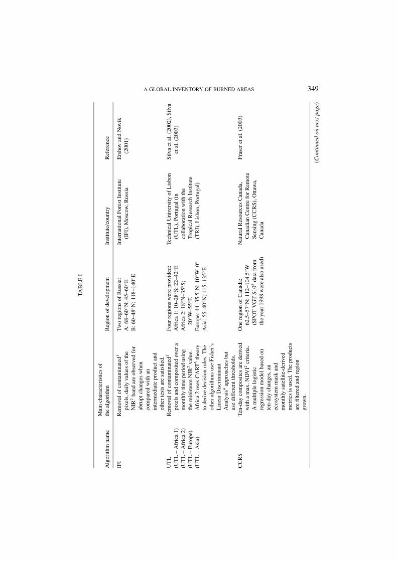
The methods required to detect a burnt area differs from one ecosystem or climaticzone to another (e.g. boreal forest, tropical forest, grasslands). Because of this,the approach taken was to develop regional algorithms, using temporal and spatialsubsets of VGT data that corresponded to each project partner’s specific region ofinterest and expertise. The main specifications of these algorithms are described inTable I. Seven algorithms were selected for processing the entire year 2000 datasetand integrated into a global processing chain (Tansey, 2002). The global dataset wasdistributed into sections depending on large-scale vegetation features or seasonalburning activity. The selection of a suitable algorithm for operational implementa-tion outside regions of algorithm calibration described in Table I was made afterlooking at different criteria. The first criterion was to look at the main types, distri-bution and patterns of vegetation in the region (needleleaf forest, broadleaf forest,grasslands etc.) using a global land cover map and select an algorithm that has beendeveloped and successfully applied over a region with similar characteristics. Asecond criterion was to apply two or three different algorithms to the same area,see how they compared between themselves and also compared to other sources ofburned area or active fire information. A third criteria depended on certain char-acteristics of the region of interest such as topography, presence of agriculturalareas, areas tending to flood and urban areas that can all have an influence on thealgorithm’s results. In a number of regions, it was necessary to use two algorithmsto fully capture all of the burning activity. This necessity was driven by evidence ofburning activity in daily images (smoke or active fires observed) or through using
A GLOBAL INVENTORY OF BURNED AREAS 349TA
BL
EI
Mai
nch
arac
teri
stic
sof
Alg
orith
mna
me
the
algo
rith
mR
egio
nof
deve
lopm
ent
Inst
itute
/cou
ntry
Ref
eren
ce
IFI
Rem
oval
ofco
ntam
inat
ed1
pixe
ls,d
aily
valu
esof
the
NIR
2ba
ndar
eob
serv
edfo
rab
rupt
chan
ges
whe
nco
mpa
red
with
anin
term
edia
tepr
oduc
tand
othe
rte
sts
are
satis
fied.
Two
regi
ons
ofR
ussi
a:A
:68–
60◦ N
;45–
60◦ E
B:6
0–48
◦ N;1
18–1
40◦ E
Inte
rnat
iona
lFor
estI
nstit
ute
(IFI
),M
osco
w,R
ussi
aE
rsho
van
dN
ovik
(200
1)
UT
L(U
TL
–A
fric
a1)
(UT
L–
Afr
ica
2)(U
TL
–E
urop
e)(U
TL
–A
sia)
Rem
oval
ofco
ntam
inat
ed1
pixe
lsan
dco
mpo
site
dov
era
mon
thly
time
peri
odus
ing
the
min
imum
NIR
2va
lue.
Afr
ica
2us
esC
AR
T3
theo
ryto
deri
vede
cisi
onru
les.
The
othe
ral
gori
thm
sus
eFi
sher
’sL
inea
rD
iscr
imin
ant
Ana
lysi
s4ap
proa
ches
but
use
diff
eren
tthr
esho
lds.
Four
regi
ons
wer
epr
ovid
ed:
Afr
ica
1:10
–28◦ S
;22–
42◦ E
Afr
ica
2:18
◦ N–3
5◦ S;
20◦ W
–55◦ E
Eur
ope:
44–3
5.5◦ N
;10◦ W
–0◦
Asi
a:55
–40◦ N
;115
–135
◦ E
Tech
nica
lUni
vers
ityof
Lis
bon
(UT
L),
Port
ugal
(in
colla
bora
tion
with
the
Tro
pica
lRes
earc
hIn
stitu
te(T
RI)
,Lis
bon,
Port
ugal
)
Silv
aet
al.(
2002
),Si
lva
etal
.(20
03)
CC
RS
Ten-
day
com
posi
tes
are
deri
ved
with
am
ax.N
DV
I2cr
iteri
a.A
mul
tiple
logi
stic
regr
essi
onm
odel
base
don
ten-
day
chan
ges,
anec
osys
tem
mas
kan
dm
onth
lysa
telli
te-d
eriv
edm
etri
csis
used
.The
prod
ucts
are
filte
red
and
regi
ongr
own.
One
regi
onof
Can
ada:
62.5
–57◦ N
;112
–104
.5◦ W
(SPO
TV
GT
S105
data
from
the
year
1998
wer
eal
sous
ed)
Nat
ural
Res
ourc
esC
anad
a,C
anad
ian
Cen
tre
for
Rem
ote
Sens
ing
(CC
RS)
,Otta
wa,
Can
ada
Fras
eret
al.(
2003
)
(Con
tinu
edon
next
page
)

350 KEVIN TANSEY ET AL.TA
BL
EI
(Con
tinu
ed)
Mai
nch
arac
teri
stic
sof
Alg
orith
mna
me
the
algo
rith
mR
egio
nof
deve
lopm
ent
Inst
itute
/cou
ntry
Ref
eren
ce
UO
E/U
TL
Rem
oval
ofco
ntam
inat
ed1
pixe
lsan
dco
mpo
site
dov
era
mon
thus
ing
the
3rd
min
.N
IR2
valu
e.T
heal
gori
thm
uses
CA
RT
3th
eory
tode
rive
deci
sion
rule
sfr
omtr
aini
ngse
ts.
One
regi
onof
Bra
zil:
5◦ N–2
0◦ S;7
5–45
◦ WU
nive
rsity
ofE
vora
,Por
tuga
l;U
TL
,Por
tuga
l;T
RI,
Port
ugal
Silv
aet
al.(
2002
)
GV
M(d
evel
oped
bySt
ropp
iana
)R
emov
alof
cont
amin
ated
1
pixe
lsan
dco
mpo
site
dov
era
ten-
day
time
peri
odus
ing
the
min
imum
NIR
2va
lue.
The
algo
rith
mus
esC
AR
T3
theo
ryto
deri
vede
cisi
onru
les
from
trai
ning
sets
.The
resu
lting
prod
ucts
are
filte
red
and
sum
med
tocr
eate
mon
thly
prod
ucts
.
One
regi
onof
Aus
tral
ia:
11–2
1◦ S;1
25–1
35◦ E
EC
Join
tRes
earc
hC
entr
e(J
RC
),Is
pra
(VA
),It
aly
Stro
ppia
naet
al.(
2002
)St
ropp
iana
etal
.(20
03)
NR
IA
chan
gede
tect
ion
algo
rith
mus
ing
pre-
and
post
-bur
nda
tain
the
NIR
2an
dSW
IR2
band
s.T
hepr
e-bu
rnim
age
isup
date
dda
ilyw
ithno
n-co
ntam
inat
edpi
xels
.To
redu
ceth
eva
riat
ion
ofth
esp
ectr
alsi
gnal
caus
edby
view
ing
geom
etry
the
algo
rith
mut
ilise
sda
ilyda
tain
five-
day
cycl
es.
One
regi
onof
sout
heas
tAfr
ica:
17–2
9◦ S;1
1–30
◦ EN
atur
alR
esou
rces
Inst
itute
(NR
I),U
nive
rsity
ofG
reen
wic
h,U
K
Bos
chet
tiet
al.(
2002
)
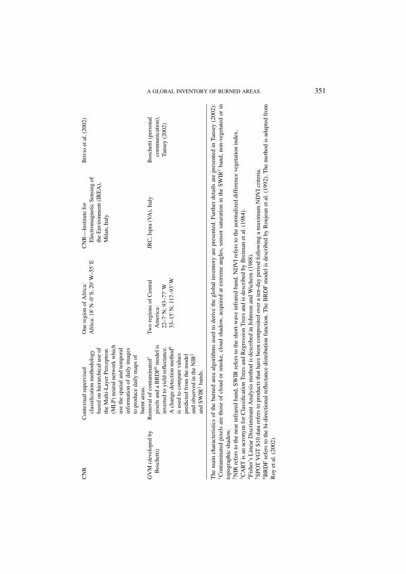
A GLOBAL INVENTORY OF BURNED AREAS 351C
NR
Con
text
uals
uper
vise
dcl
assi
ficat
ion
met
hodo
logy
base
don
hier
arch
ical
use
ofth
eM
ulti-
Lay
erPe
rcep
tron
(ML
P)ne
ural
netw
ork
whi
chus
eth
esp
atia
land
tem
pora
lin
form
atio
nof
daily
imag
esto
prod
uce
daily
map
sof
burn
tare
as.
One
regi
onof
Afr
ica:
Afr
ica:
18◦ N
–0◦ S
;20◦ W
–55◦ E
CN
R—
Inst
itute
for
Ele
ctro
mag
netic
Sens
ing
ofth
eE
nvir
onm
ent(
IRE
A),
Mila
n,It
aly
Bri
vio
etal
.(20
02)
GV
M(d
evel
oped
byB
osch
etti)
Rem
oval
ofco
ntam
inat
ed1
pixe
lsan
da
BR
DF6
mod
elis
inve
rted
toyi
eld
refle
ctan
ce.
Ach
ange
dete
ctio
nm
etho
d6
isus
edto
com
pare
valu
espr
edic
ted
from
the
mod
elan
dob
serv
edin
the
NIR
2
and
SWIR
2ba
nds.
Two
regi
ons
ofC
entr
alA
mer
ica:
22–7
◦ N;9
3–77
◦ W33
–15◦ N
;117
–93◦ W
JRC
,Isp
ra(V
A),
Ital
yB
osch
etti
(per
sona
lco
mm
unic
atio
n),
Tans
ey(2
002)
The
mai
nch
arac
teri
stic
sof
the
burn
edar
eaal
gori
thm
sus
edto
deri
veth
egl
obal
inve
ntor
yar
epr
esen
ted.
Furt
her
deta
ilsar
epr
esen
ted
inTa
nsey
(200
2):
1C
onta
min
ated
pixe
lsar
eth
ose
ofcl
oud
orsm
oke,
clou
dsh
adow
,acq
uire
dat
extr
eme
angl
es,s
enso
rsa
tura
tion
inth
eSW
IR2
band
,non
-veg
etat
edor
into
pogr
aphi
csh
adow
.2N
IRre
fers
toth
ene
arin
frar
edba
nd,S
WIR
refe
rsto
the
shor
t-w
ave
infr
ared
band
.ND
VI
refe
rsto
the
norm
aliz
eddi
ffer
ence
vege
tatio
nin
dex.
3C
AR
Tis
anac
rony
mfo
rC
lass
ifica
tion
Tre
esan
dR
egre
ssio
nT
rees
and
isde
scri
bed
byB
reim
anet
al.(
1984
).4Fi
sher
’sL
inea
rD
iscr
imin
antA
naly
sis
met
hod
isde
scri
bed
inJo
hnso
nan
dW
iche
rn(1
988)
.5SP
OT
VG
TS1
0da
tare
fers
topr
oduc
tsth
atha
vebe
enco
mpo
site
dov
era
ten-
day
peri
odfo
llow
ing
am
axim
umN
DV
Icr
iteri
a.6B
RD
Fre
fers
toth
ebi
-dir
ectio
nalr
eflec
tanc
edi
stri
butio
nfu
nctio
n.T
heB
RD
Fm
odel
isde
scri
bed
byR
ouje
anet
al.(
1992
).T
hem
etho
dis
adap
ted
from
Roy
etal
.(20
02).
352 KEVIN TANSEY ET AL.
higher resolution images such as from Landsat TM quick-looks available freelythrough the Internet (http://Glovis.usgs.gov/BrowseBrowser.shtml). Tansey (2002)provides a complete overview of the spatial and temporal application of the GBAalgorithms that is summarized in the next three paragraphs.
The CCRS algorithm was used to derive burned area products for forested re-gions of Canada and the United States (US) (according to a forest cover mapprovided by CCRS). The non-forested regions of the US were processed using thefirst algorithm developed by the UTL group (UTL Africa 1). Southern regions ofthe US and Central America are processed with the IFI and GVM (developed byBoschetti) algorithms. A window covering the northern half of the South Americancontinent (including the Amazon Forest) was processed with a dedicated algorithmdeveloped by UOE/UTL. The southern half of South America (including Argentinaand Chile) was processed solely using the IFI algorithm. After a long period of test-ing with several algorithms, a single algorithm (UTL Africa 2) was used to derivethe burned area products for sub-Saharan Africa. In northern Europe and Asia (in-cluding the majority of Russia), the IFI algorithm was solely used. However, furthersouth down to 30◦N, the IFI algorithm was used in unison with other algorithms,namely the UTL Europe algorithm for southern Europe and northern Africa, UTLAfrica 2 in Turkey, Iraq and regions surrounding the Black and Caspian Seas andthe UTL Asia (a derivative of UTL Africa 1) for a large region stretching betweenthe Tibetan Plateau in the west through Mongolia and China to Japan in the east.The Indian sub-continent, southern China, continental and insular Southeast Asiawere processed solely with the IFI algorithm. Australia was processed with an al-gorithm developed by GVM (developed by Stroppiana). Certain regions were notconsidered at all in the GBA, 2000 project because of their isolated location ortheir insignificant contribution to global burning activity. These regions includeNew Zealand and many small Pacific Islands, northern England, Scotland, Eire,Northern Ireland, Hawaii, Iceland and Greenland. The merits and performance ofeach of these algorithms is presented in Tansey (2002).
In certain regions, the algorithms were not applied to the VGT dataset for thewhole of the year 2000. These regions were characterized by distinct fire seasonscaused mainly by climatic variations (snow cover, heavy rainfall etc.). In more thanone case, when the algorithms were applied to the VGT data outside the main periodsof fire activity then false detections were observed, most commonly due to flooding.Information was used from published literature and other sources, for examplethe World Fire Web (Dwyer et al., 1999) to define the main periods of burningactivity. To summarize, the main period of burning activity regions lying north of30◦N correspond to the Northern Hemisphere summer period, therefore data wereprocessed between April and October 2000. South of this region and approximatelybetween 30◦N and 8◦N in Central America, 30◦N and 10◦N in Africa and 30◦N and6◦N in India and Southeast Asia the main period of burning activity is associatedwith the Northern Hemisphere dry season (winter), therefore data were processedbetween January and May 2000 and again from September to December 2000. In

A GLOBAL INVENTORY OF BURNED AREAS 353
the equatorial region and Southern Hemisphere the burning season is less distinct,apart from in Africa. In southern Africa, between approximately 10◦S and the Capeof Good Hope in South Africa, the main period of burning is associated with theSouthern Hemisphere dry season (winter), therefore data were processed betweenApril and December 2000. The annual dataset was processed for all other regionsincluding South America south of 10◦N, equatorial Africa between 10◦N and 10◦Sand insular Southeast Asia and Australia south of 6◦N. In these regions there ispotential for significant burning activity at any time of the year. The inventorydescribed in the paper contains monthly burned area products and a synthesis ofthe total annual burned area for the year 2000 (the latter indicating those pixelsdetected as burned one or more times during the year 2000). During the processingof the data the monthly products were made non-accumulative. The assumptionthat, a vegetated surface burns only once during the year, is made in most regions.However, this is not always true, for example in Africa, in countries such as Chad,Sudan and Ethiopia, it may be that a vegetated area is burned towards the end ofthe 1999–2000 dry season so is detected in January 2000 and after the wet seasonand vigorous vegetation growth during this time, the vegetation is again burnedearlier in the 2000–2001 dry season and is detected in December 2000. Therefore,a caution is given to the user when using the year 2000 synthesis product. Thisproduct may yield the total area burned during the year 2000, but if the user isusing the product to infer burned biomass or emissions then errors are potentiallyintroduced through an underestimation. The phenomenon of two detections duringthe year 2000 only affects those regions between 0 and 30◦N. The ability to detectburnt areas that occur beneath a vegetated canopy that has not been burnt needsto be mentioned. It is believed that these burn scars are not detected by the VGTsensor because the main component of the radiant signal is coming from the partof the vegetation canopy that has not burnt. The chance of detecting the burn scarincreases significantly as the density of the canopy decreases. Pereira et al. (inpress) presents a discussion of this topic.
The masking of contaminated pixels before applying the algorithms was a nec-essary step for several of the algorithms. Contaminated pixels having values charac-teristic of clouds, cloud shadow (that have similar spectral characteristics to burnedareas) and fire smoke are removed. In addition, those pixels located at the very edgeof the image swath are removed because often they have erroneous values causedby the resampling method and also those that appear to be saturated (or have veryhigh values of reflectance) in the short-wave infrared band caused by problems withthe sensor. It was discovered that in regions of pronounced topographical variation,such as the Himalayas and the Andes, pixels were falsely being detected as beingburnt in areas of terrain shadow. To solve this problem, a digital elevation model (aDEM from the Global Land One-km Base Elevation (GLOBE) product (Hastingsand Dunbar, 1998) from http://www.ndgc.noaa.gov/seg/topo/globe.shtml), regis-tered to the VGT S1 dataset was used. The method used to determine those pixelscontaminated by terrain shadow is given by Colby (1991) and uses sun zenith and
354 KEVIN TANSEY ET AL.
azimuth information on a pixel basis provided in the VGT S1 product as well as slopeand aspect information from the DEM. After determining the contaminated pixels,they were dilated by one-pixel in all directions to ensure that all shadow-affectedpixels were removed. The terrain shadow masks were produced on a daily basis.Information on land cover at a global scale was used in this study for a number of rea-sons. A land cover product provides a mask to remove non-vegetated surfaces suchas water, urban areas, deserts (including the Sahara, Kalahari, Arabian Peninsula,Tibetan Plateau and Atacama deserts) and ice masses that can otherwise cause prob-lems and uncertainties in the performance of the algorithms. A land cover productprovides guidance in the selection of an algorithm that is to be applied to a region ofinterest outside the region in which the algorithm was developed and calibrated. Theglobal land cover product selected for this study was the University of Maryland(UMD) global land cover product (Hansen et al., 2000). The UMD product wasselected because during the time that this study was undertaken it was considered tobe the most current product that was freely available to the users (http://glcf.umiacs.umd.edu/data.html) and actively being used by many different research groups.
4. Analysis and Discussion of the GBA, 2000 Inventory
The inventory described in this paper consists of one annual and twelve monthlyproducts of burned areas at a resolution of 1 km. A detailed description is given of thespatial and temporal distribution of burned areas in the year 2000 overlapped withpolitical boundaries. This method of reporting may primarily appeal to the policydecision-making community, but we believe that reporting the statistics in this waywill best demonstrate the value of the GBA, 2000 dataset and encourage other usersto use this data, particularly climate change and ecosystem modellers, for their ownaims and objectives. Those interested in burnt area estimates for broad vegetationcover types (forest, grasslands and croplands, savannas and woodlands) shouldrefer to Tansey et al. (2004). Following this description, discussion is presentedon placing the year 2000 into context when considering burning activity in otheryears. The final sub-section describes some of the observed errors in the GBA, 2000products and outlines validation exercises. All estimates of burned area are givenin square kilometers (km2).
4.1. SPATIAL AND TEMPORAL DISTRIBUTION OF BURNED AREAS
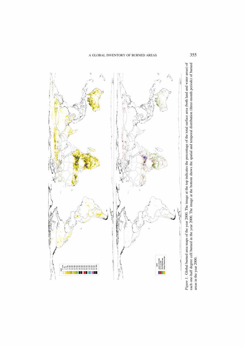
The story of biomass burning in the year 2000 is shown in Figure 1. Figure 1 (top)shows the percentage of the total surface area (land and water) of each one-halfdegree (1/2◦) cell burned in the year 2000. This parameter provides an indicationof the magnitude (or inferred intensity) of biomass burning processes in each gridcell. The values range from one percent of the surface area to one hundred percent(at 1 km resolution) burning, the latter estimate occurring in several grid cells in
A GLOBAL INVENTORY OF BURNED AREAS 355
Fig
ure
1.G
loba
lbur
ned
area
map
sof
the
year
2000
.The
imag
eat
the
top
indi
cate
sth
epe
rcen
tage
ofth
eto
tals
urfa
cear
ea(b
oth
land
and
wat
erar
eas)
ofea
chon
e-ha
lfde
gree
cell
burn
edin
the
year
2000
.The
imag
eat
the
botto
msh
ows
the
spat
ial
and
tem
pora
ldi
stri
butio
n(t
hree
-mon
thpe
riod
s)of
burn
edar
eas
inth
eye
ar20
00.
356 KEVIN TANSEY ET AL.
southern Sudan and the Central African Republic. As previously mentioned, theregion with the greatest burning activity per surface area is the Northern Hemispheresub-tropical shrubland and wooded grassland belt in Africa. With the exception ofSomalia and Nigeria (for reasons that may be worthy of further investigation)biomass burning is widespread in this region. High intensities of burning activity isobserved in the Southern Hemisphere of Africa, with peaks to be found in northernAngola and southern DR Congo (80% of the grid cell). Similar intensities can befound in northern Australia in the tropical grassland and interior regions. Moderateintensities of burning (30–60%) are observed in a number of places, including thetemperate grasslands of eastern Mongolia and northern China and in southern China,Burma and isolated regions of India. The major grassland regions of South America(the Llanos of the Orinoco in Venezuela and Colombia, the Mato Grosso in Brazil,the Llanos of Mojos in Bolivia and the Pampas in Argentina) are all observed tohave moderate intensities of burning activity. Burning activity in southwest Russia,the Ukraine and northern Kazakhstan also occurs in moderate intensities. Thisburning has been associated with agricultural practices. Other isolated hotspots aredetected across the globe. Two regions highlighted are the large forest fires detectedin Montana and Idaho States of the US in the year 2000 and the large forest fires inCanada that are large enough to represent a significant proportion of the one-halfdegree cell.
Figure 1 (bottom) shows the temporal distribution (in three month periods) of theburning activity in the year 2000 at global scale. Unlike the figure shown above it,Figure 1 (bottom) shows the actual pixels (resampled for display purposes) that weredetected as being burned. Monthly maps of burned areas can be viewed throughthe Internet, hosted by the United Nation Environment Programme (UNEP) athttp://www.grid.unep.ch/activities/earlywarning/preview/ims/gba/. In the follow-ing paragraphs, the use of the phrase ‘burning activity’ refers to the detection ofburn scars and not the detection of active fires or fire activity.
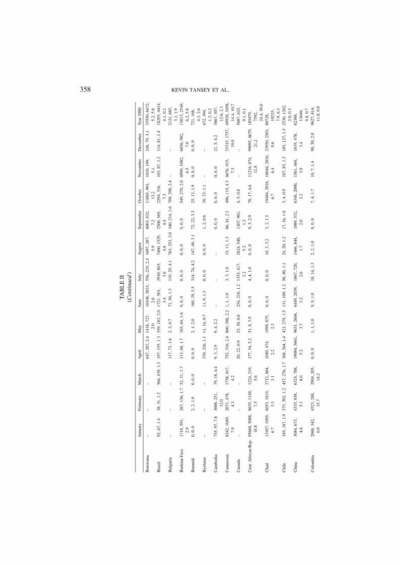
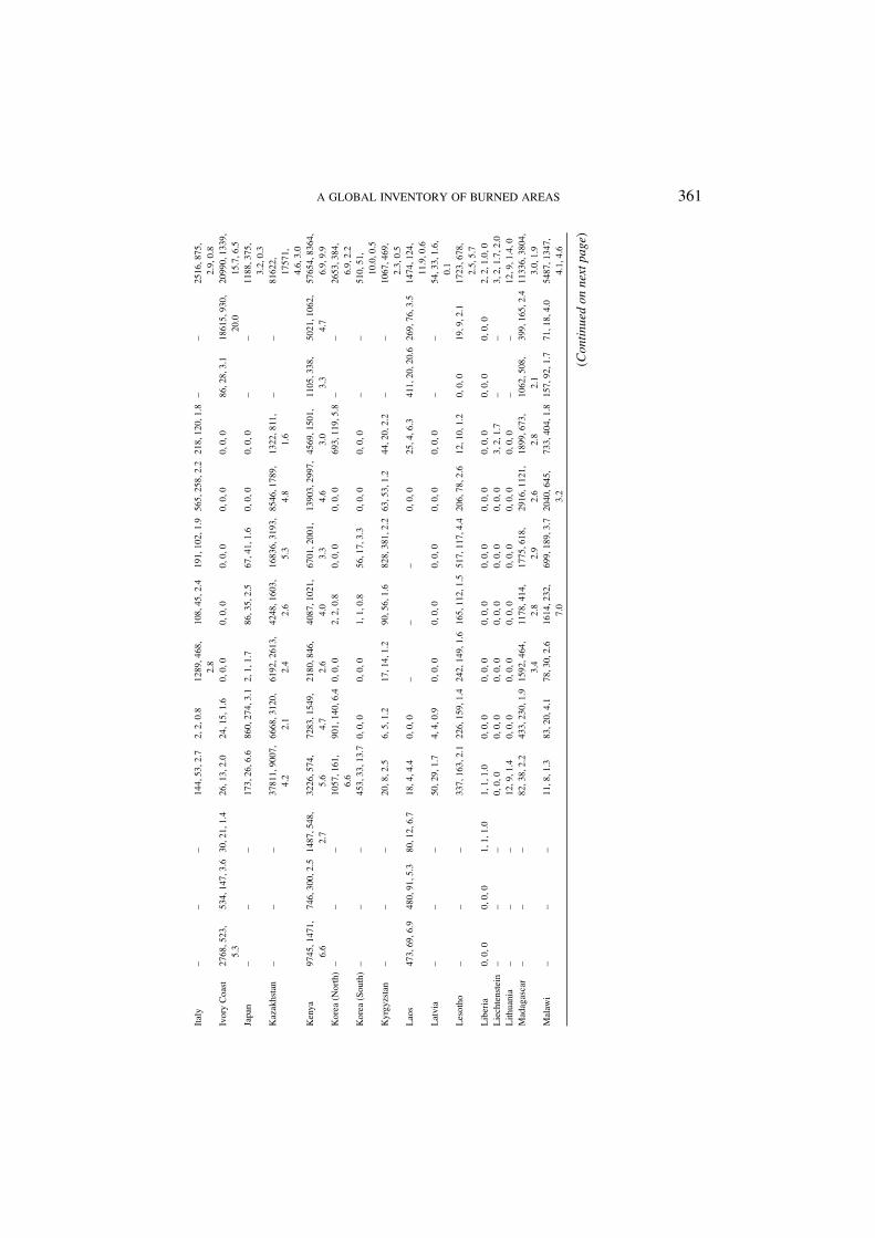
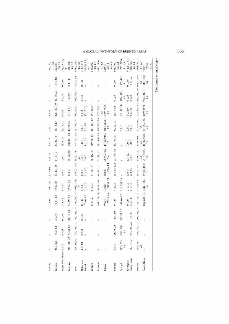
Estimates of burned area (in square kilometers) are given in Table II by politicalboundary to support the statements that are made in the text. In addition to theburned area values, figures are presented on the number of burned scars (eithersingle pixel or cluster of pixels) and the average size of a burned area (in squarekilometers) and, for the year 2000, the percentage of the total area of the country(including land and water areas). The values given in Table II are comma delimitedand are presented for each month of the year 2000 and for the year 2000 annualsynthesis. A dash (-) indicates that no burned area product was derived for thatparticular month and country. Note that only those countries with burned scarsdetected in the year 2000 are presented in Table II. Countries that are absent fromthe table either have no burned areas detected within their political boundary orwere not included when the algorithms were applied. Before an interpretation ofthe monthly distribution of burned areas is given it is worth extracting the mainthemes that are observed in the annual synthesis of the GBA, 2000 product. To helpus to extract the main themes the GBA, 2000 products are cross-referenced with a

A GLOBAL INVENTORY OF BURNED AREAS 357TA
BL
EII
Key
(com
ma
delim
ited)
:Bur
ned
area
(km
2),
num
ber
ofsc
ars,
aver
age
size
ofth
esc
ar(k
m2),
%of
tota
lare
aof
coun
try
burn
ed(s
how
nfo
rth
eye
ar20
00on
ly),
ada
sh(–
)in
dica
tes
noda
taw
ere
acqu
ired
Janu
ary
Febr
uary
Mar
chA
pril
May
June
July
Aug
ust
Sept
embe
rO
ctob
erN
ovem
ber
Dec
embe
rY
ear
2000
Afg
hani
stan
––
–19
,15,
1.2
17,1
9,0.
912
4,56
,2.2
184,
93,2
.028
1,18
9,1.
55,
2,2.
456
,53,
1.1
––
686,
320,
2.1,
0.1
Alb
ania
––
–8,
6,1.
30,
0,0
0,0,
015
,5,3
.114
,6,2
.31,
2,0.
784
,50,
1.7
––
122,
67,1
.8,
0.4
Alg
eria
––
–2,
1,1.
635
,15,
2.3
15,1
5,1.
021
,17,
1.2
377,
80,4
.788
3,17
4,5.
117
1,92
,1.9
––
1503
,251
,6.
0,0.
1A
ngol
a14
,1,1
3.6
5,3,
1.6
7,3,
2.3
2670
,432
,6.
249
94,8
87,
5.6
7034
1,43
99,1
6.0
1124
82,
8415
,13.
466
005,
7950
,8.3
3315
8,61
94,5
.451
65,1
380,
3.7
1212
,406
,3.
051
1,17
3,3.
029
6545
,20
286,
14.6
,23.
7A
rgen
tina
3168
,119
5,2.
730
49,1
558,
2.0
2468
,103
2,2.
439
72,1
921,
2.1
8807
,356
5,2.
541
57,2
140,
1.9
7653
,338
2,2.
351
73,2
905,
1.8
5559
,237
2,2.
315
74,6
88,
2.3
3194
,112
0,2.
966
96,8
86,
7.6
5546
8,16
717,
3.3,
2.0
Arm
enia
––
–61
,28,
2.2
0,0,
02,
1,2.
36,
5,1.
29,
6,1.
50,
0,0
0,0,
0–
–79
,38,
2.1,
0.3
Aus
tral
ia45
263,
2777
,16.
327
515,
2086
,13.
216
924,
1672
,10.
110
740,
1207
,8.9
1399
5,11
69,1
2.0
2258
1,15
69,1
4.4
2816
7,14
80,1
9.0
6961
6,16
66,4
1.8
1403
93,
2314
,60.
784
243,
2601
,32.
485
698,
3984
,21.
513
732,
957,
14.3
5588
67,
1969
3,28
.4,7
.3A
ustr
ia–
––
4,1,
4.0
0,0,
00,
0,0
5,4,
1.2
1,1,
0.7
34,3
7,0.
953
,26,
2.0
––
96,6
8,1.
4,0.
1A
zerb
aija
n–
––
189,
63,3
.018
,14,
1.3
31,1
4,2.
214
3,51
,2.8
146,
49,3
.00,
0,0
4,3,
1.3
––
531,
174,
3.1,
0.6
Bah
amas
0,0,
00,
0,0
0,0,
07,
2,3.
51,
1,0.
9–
––
0,0,
00,
0,0
1,1,
0.9
0,0,
09,
4,2.
2,0.
1B
angl
ades
h66
,12,
5.5
17,1
3,1.
324
,5,4
.743
,5,8
.711
,2,5
.4–
––
0,0,
03,
2,1.
359
,7,8
.554
,9,6
.027
7,49
,5.7
,0.
2B
elgi
um–
––
10,1
,9.6
0,0,
00,
0,0
0,0,
00,
0,0
0,0,
00,
0,0
––
10,1
,9.6
,0B
eliz
e0,
0,0
0,0,
00,
0,0
0,0,
00,
0,0
––
–0,
0,0
0,0,
00,
0,0
1,1,
0.9
1,1,
0.9,
0B
enin
1581
,347
,4.
628
2,11
3,2.
54,
3,1.
354
,32,
1.7
15,7
,2.1
1,1,
1.0
0,0,
00,
0,0
3,3,
1.0
0,0,
017
69,1
89,
9.4
9943
,805
,12
.413
003,
1194
,10
.9,1
1.2
Bhu
tan
3,3,
1.2
3,2,
1.7
15,4
,3.7
52,8
,6.4
0,0,
0–
––
0,0,
026
,7,3
.724
,10,
2.4
33,1
4,2.
415
6,46
,3.4
,0.
4B
oliv
ia36
,23,
1.6
49,3
5,1.
422
,22,
1.0
186,
146,
1.3
786,
447,
1.8
360,
248,
1.5
2196
,608
,3.
616
51,5
14,
3.2
3516
,477
,7.
468
5,14
9,4.
638
3,19
5,2.
031
5,17
7,1.
810
185,
2539
,4.0
,0.
9
(Con
tinu
edon
next
page
)
358 KEVIN TANSEY ET AL.
TAB
LE
II(C
onti
nued
)
Janu
ary
Febr
uary
Mar
chA
pril
May
June
July
Aug
ust
Sept
embe
rO
ctob
erN
ovem
ber
Dec
embe
rY
ear
2000
Bot
swan
a–
––
647,
267,
2.4
1418
,727
,2.
010
106,
3833
,2.
655
6,23
5,2.
416
97,2
87,
5.9
6003
,832
,7.
211
865,
901,
13.2
1010
,199
,5.
124
8,79
,3.1
3355
0,64
72,
5.2,
5.8
Bra
zil
92,6
7,1.
438
,31,
1.2
566,
439,
1.3
197,
155,
1.3
359,
183,
2.0
1721
,501
,3.
429
10,8
03,
3.6
7400
,152
9,4.
825
00,5
65,
4.4
2294
,316
,7.
310
3,87
,1.2
114,
81,1
.418
293,
4414
,4.
1,0.
2B
ulga
ria
––
–11
7,73
,1.6
2,3,
0.7
71,5
6,1.
311
9,29
,4.1
763,
253,
3.0
340,
214,
1.6
709,
290,
2.4
––
2121
,685
,3.
1,1.
9B
urki
naFa
so17
18,5
91,
2.9
267,
156,
1.7
52,3
1,1.
711
3,68
,1.7
103,
64,1
.60,
0,0
0,0,
00,
0,0
0,0,
054
9,27
0,2.
069
99,1
082,
6.5
6856
,982
,7.
015
813,
2549
,6.
2,5.
8B
urun
di0,
0,0
2,2,
1.0
0,0,
00,
0,0
2,1,
2.0
160,
29,5
.531
4,74
,4.2
147,
48,3
.172
,22,
3.3
25,1
3,1.
90,
0,0
0,0,
072
1,16
8,4.
3,2.
6B
yela
rus
––
–37
0,32
6,1.
111
,16,
0.7
11,9
,1.3
0,0,
00,
0,0
1,2,
0.6
78,7
3,1.
1–
–47
2,39
4,1.
2,0.
2C
ambo
dia
755,
97,7
.830
06,2
51,
12.0
79,1
8,4.
49,
3,2.
99,
4,2.
2–
––
0,0,
00,
0,0
0,0,
021
,5,4
.238
67,3
07,
12.6
,2.1
Cam
eroo
n82
42,1
049,
7.9
2071
,478
,4.
317
56,4
17,
4.2
752,
316,
2.4
860,
386,
2.2
1,1,
1.0
3,3,
1.0
15,1
1,1.
386
,41,
2.1
496,
115,
4.3
6676
,915
,7.
333
315,
1757
,19
.049
928,
3458
,14
.4,1
0.7
Can
ada
––
–20
,22,
0.9
23,3
0,0.
825
4,21
0,1.
213
55,4
17,
3.2
2824
,548
,5.
212
07,9
01,
1.3
4,5,
0.8
––
5687
,625
,9.
1,0.
1C
ent.
Afr
ican
Rep
.95
668,
5088
,18
.886
35,1
149,
7.5
1224
,219
,5.
617
7,34
,5.2
31,8
,3.9
0,0,
04,
4,1.
00,
0,0
9,3,
2.9
78,1
7,4.
611
216,
874,
12.8
9909
5,46
79,
21.2
1854
79,
7592
,24
.4,3
0.0
Cha
d13
457,
1995
,6.
760
53,1
819,
3.3
2712
,884
,3.
110
49,4
74,
2.2
1999
,875
,2.
30,
0,0
0,0,
010
,3,3
.23,
2,1.
519
484,
2916
,6.
718
046,
2816
,6.
423
950,
2503
,9.
680
728,
1023
5,7.
9,6.
3C
hile
349,
187,
1.9
375,
302,
1.2
457,
276,
1.7
368,
264,
1.4
421,
279,
1.5
131,
109,
1.2
98,9
0,1.
124
,20,
1.2
17,1
6,1.
03,
4,0.
910
7,83
,1.3
185,
127,
1.5
2536
,128
2,2.
0,0.
3C
hina
3084
,673
,4.
643
35,8
58,
5.1
6324
,788
,8.
019
084,
3661
,5.
296
31,2
606,
3.7
6449
,203
9,3.
218
67,7
20,
2.6
1466
,844
,1.
710
89,5
32,
2.0
6348
,200
0,3.
215
61,4
04,
3.9
1619
,478
,3.
462
388,
1304
9,4.
8,0.
7C
olom
bia
2068
,342
,6.
045
23,2
88,
15.7
2904
,205
,14
.20,
0,0
1,1,
1.0
9,9,
1.0
18,1
4,1.
32,
2,1.
00,
0,0
7,4,
1.7
10,7
,1.4
98,5
0,2.
096
27,8
14,
11.8
,0.8

A GLOBAL INVENTORY OF BURNED AREAS 359C
omor
os–
––
11,6
,1.8
10,5
,1.9
2,2,
1.0
1,1,
1.0
11,4
,2.6
1,1,
1.0
1,1,
1.0
––
36,1
3,2.
7,2.
2C
ongo
28,1
5,1.
929
,18,
1.6
79,4
0,2.
089
,29,
3.1
40,1
3,3.
126
6,40
,6.6
1221
,245
,5.
012
11,2
96,
4.1
1492
,195
,7.
710
21,6
6,15
.538
1,85
,4.5
5,5,
1.0
5810
,797
,7.
3,1.
7C
osta
Ric
a0,
0,0
3,2,
1.4
0,0,
044
,13,
3.4
0,0,
0–
––
0,0,
00,
0,0
4,3,
1.3
0,0,
051
,18,
2.8,
0.1
Cub
a50
,18,
2.8
130,
47,2
.882
,26,
3.1
190,
65,2
.955
,17,
3.3
––
–0,
0,0
0,0,
07,
3,2.
43,
3,0.
951
3,14
4,3.
6,0.
5C
ypru
s–
––
0,0,
04,
3,1.
320
,5,4
.00,
0,0
2,2,
0.8
0,0,
00,
0,0
––
26,1
0,2.
6,0.
3C
zech
Rep
–Slo
vak.
––
–34
,14,
2.5
0,0,
01,
2,0.
70,
0,0
0,0,
020
,15,
1.3
143,
51,2
.8–
–19
9,78
,2.6
,0.
2D
em.R
ep.C
ongo
1528
8,14
04,
10.9
6763
,109
4,6.
218
66,3
60,
5.2
295,
145,
2.0
2622
5,29
80,
8.8
9047
8,69
52,
13.0
8773
9,71
78,
12.2
2426
5,25
90,
9.4
3653
,796
,4.
647
6,17
6,2.
749
0,17
9,2.
745
88,4
69,
9.8
2600
32,
1561
4,16
.7,1
1.2
Djib
outi
7,6,
1.1
94,2
0,4.
70,
0,0
6,4,
1.4
5,2,
2.4
––
–0,
0,0
317,
37,8
.627
,13,
2.1
0,0,
042
1,45
,9.4
,2.
0D
omin
ican
Rep
.1,
1,0.
94,
3,1.
27,
5,1.
30,
0,0
0,0,
0–
––
0,0,
00,
0,0
3,2,
1.4
2,2,
0.9
16,1
2,1.
3,0
Ecu
ador
6,6,
1.0
25,2
0,1.
213
,13,
1.0
3,2,
1.5
4,4,
1.0
28,2
5,1.
142
,29,
1.5
30,2
2,1.
413
,9,1
.411
,5,2
.27,
7,1.
016
,11,
1.4
197,
138,
1.4,
0.1
Egy
pt–
––
18,7
,2.5
812,
83,9
.878
,45,
1.7
4,4,
1.1
0,0,
00,
0,0
0,0,
0–
–91
2,12
5,7.
3,0.
1E
lSal
vado
r9,
5,1.
75,
4,1.
20,
0,0
0,0,
00,
0,0
––
–0,
0,0
0,0,
03,
1,2.
93,
3,1.
016
,6,2
.7,
0.1
Equ
ator
ialG
uine
a11
,2,5
.40,
0,0
0,0,
07,
5,1.
40,
0,0
0,0,
00,
0,0
0,0,
00,
0,0
2,1,
2.0
0,0,
00,
0,0
19,6
,3.1
,0.
1E
ston
ia–
––
7,11
,0.7
17,1
4,1.
21,
1,0.
50,
0,0
0,0,
01,
1,0.
50,
0,0
––
25,2
6,1.
0,0.
1E
thio
pia
2934
4,24
82,
11.8
1990
6,24
19,
8.2
2216
0,25
40,
8.7
1147
0,26
21,
4.4
6288
,156
5,4.
026
84,7
48,
3.6
3234
,124
6,2.
610
504,
2412
,4.
443
74,1
588,
2.8
4124
,124
4,3.
387
64,1
428,
6.1
2934
1,44
29,
6.6
1409
19,
1566
0,9.
0,11
.3Fi
nlan
d–
––
7,11
,0.7
78,1
24,0
.610
,17,
0.6
4,6,
0.7
0,1,
0.3
0,0,
00,
0,0
––
99,1
58,0
.6,
0Fr
ance
––
–80
,35,
2.3
1,1,
0.7
13,1
4,0.
959
,45,
1.3
48,3
5,1.
423
8,11
5,2.
111
7,84
,1.4
––
555,
282,
2.0,
0.1
Fren
chG
uian
a0,
0,0
0,0,
00,
0,0
0,0,
00,
0,0
1,1,
1.0
0,0,
00,
0,0
0,0,
00,
0,0
0,0,
00,
0,0
1,1,
1.0,
0G
abon
22,1
2,1.
821
,6,3
.412
,8,1
.547
,14,
3.4
58,1
0,5.
84,
2,2.
010
5,32
,3.3
534,
136,
3.9
4,1,
3.9
0,0,
00,
0,0
0,0,
080
5,19
9,4.
0,0.
3
(Con
tinu
edon
next
page
)

360 KEVIN TANSEY ET AL.
TAB
LE
II(C
onti
nued
)
Janu
ary
Febr
uary
Mar
chA
pril
May
June
July
Aug
ust
Sept
embe
rO
ctob
erN
ovem
ber
Dec
embe
rY
ear
2000
Gam
bia
79,1
8,4.
447
7,40
,11.
963
,17,
3.7
24,1
4,1.
711
4,63
,1.8
––
–0,
0,0
4,3,
1.3
72,2
1,3.
421
,12,
1.7
814,
148,
5.5,
7.6
Geo
rgia
––
–59
,17,
3.4
12,7
,1.8
15,8
,1.9
28,1
2,2.
361
,45,
1.4
0,0,
05,
3,1.
7–
–18
1,85
,2.1
,0.
3G
erm
any
––
–25
,16,
1.6
3,3,
1.0
0,0,
00,
0,0
7,2,
3.4
22,1
0,2.
213
,12,
1.1
––
70,3
9,1.
8,0
Gha
na97
75,1
933,
5.1
1024
,369
,2.
816
7,87
,1.9
23,1
7,1.
443
,23,
1.9
0,0,
03,
2,1.
50,
0,0
0,0,
012
,11,
1.1
4398
,531
,8.
342
073,
1372
,30
.753
747,
2374
,22
.6,2
2.5
Gre
ece
––
–12
,5,2
.42,
2,1.
229
,29,
1.0
469,
46,1
0.2
186,
31,6
.071
,37,
1.9
396,
118,
3.4
––
1165
,231
,5.
0,0.
9G
uate
mal
a36
,28,
1.3
54,3
9,1.
45,
3,1.
645
,12,
3.8
0,0,
0–
––
0,0,
00,
0,0
0,0,
013
,7,1
.915
2,82
,1.9
,0.
1G
uine
a21
74,6
13,
3.5
1532
,452
,3.
414
6,64
,2.3
53,2
3,2.
39,
7,1.
20,
0,0
0,0,
00,
0,0
0,0,
046
,14,
3.3
287,
91,3
.239
23,7
57,
5.2
7999
,180
7,4.
4,3.
3G
uine
a–B
issa
u10
0,33
,3.0
197,
66,3
.04,
3,1.
314
,6,2
.439
,23,
1.7
––
–0,
0,0
0,0,
037
,22,
1.7
13,9
,1.5
393,
145,
2.7,
1.2
Guy
ana
0,0,
01,
1,1.
00,
0,0
0,0,
00,
0,0
1,1,
1.0
1,1,
1.0
0,0,
00,
0,0
0,0,
00,
0,0
0,0,
03,
3,1.
0,0
Hai
ti7,
3,2.
514
,5,2
.81,
1,0.
90,
0,0
0,0,
0–
––
0,0,
00,
0,0
0,0,
02,
1,1.
922
,8,2
.8,
0.1
Hon
dura
s2,
2,1.
013
,2,6
.70,
0,0
2,2,
1.0
0,0,
0–
––
0,0,
00,
0,0
0,0,
01,
1,1.
018
,7,2
.6,0
Hun
gary
––
–52
,50,
1.0
16,1
5,1.
114
,18,
0.8
4,4,
1.0
99,5
5,1.
864
0,31
0,2.
155
4,27
1,2.
0–
–13
78,5
50,
2.5,
1.5
Indi
a39
17,4
55,
8.6
3066
,496
,6.
212
937,
1075
,12
.095
49,1
011,
9.4
8917
,878
,10
.20,
0,0
0,0,
037
,6,6
.155
5,75
,7.4
3179
,606
,5.
229
22,3
56,
8.2
5399
,670
,8.
147
134,
3268
,14
.4,1
.5In
done
sia
12,2
,5.9
10,2
,4.9
6,3,
2.0
57,3
,18.
915
,2,7
.366
,6,1
1.1
77,1
6,4.
851
3,75
,6.8
916,
107,
8.6
204,
23,8
.916
,3,5
.211
,3,3
.619
02,1
88,
10.1
,0.1
Iran
––
–62
0,23
5,2.
630
,21,
1.5
99,6
0,1.
610
0,57
,1.7
185,
103,
1.8
0,0,
08,
2,3.
9–
–10
42,4
18,
2.5,
0.1
Iraq
––
–17
,11,
1.5
6,6,
0.9
0,0,
00,
0,0
22,1
1,2.
00,
0,0
0,0,
0–
–44
,28,
1.6,
0
A GLOBAL INVENTORY OF BURNED AREAS 361It
aly
––
–14
4,53
,2.7
2,2,
0.8
1289
,468
,2.
810
8,45
,2.4
191,
102,
1.9
565,
258,
2.2
218,
120,
1.8
––
2516
,875
,2.
9,0.
8Iv
ory
Coa
st27
68,5
23,
5.3
534,
147,
3.6
30,2
1,1.
426
,13,
2.0
24,1
5,1.
60,
0,0
0,0,
00,
0,0
0,0,
00,
0,0
86,2
8,3.
118
615,
930,
20.0
2099
0,13
39,
15.7
,6.5
Japa
n–
––
173,
26,6
.686
0,27
4,3.
12,
1,1.
786
,35,
2.5
67,4
1,1.
60,
0,0
0,0,
0–
–11
88,3
75,
3.2,
0.3
Kaz
akhs
tan
––
–37
811,
9007
,4.
266
68,3
120,
2.1
6192
,261
3,2.
442
48,1
603,
2.6
1683
6,31
93,
5.3
8546
,178
9,4.
813
22,8
11,
1.6
––
8162
2,17
571,
4.6,
3.0
Ken
ya97
45,1
471,
6.6
746,
300,
2.5
1487
,548
,2.
732
26,5
74,
5.6
7283
,154
9,4.
721
80,8
46,
2.6
4087
,102
1,4.
067
01,2
001,
3.3
1390
3,29
97,
4.6
4569
,150
1,3.
011
05,3
38,
3.3
5021
,106
2,4.
757
654,
8364
,6.
9,9.
9K
orea
(Nor
th)
––
–10
57,1
61,
6.6
901,
140,
6.4
0,0,
02,
2,0.
80,
0,0
0,0,
069
3,11
9,5.
8–
–26
53,3
84,
6.9,
2.2
Kor
ea(S
outh
)–
––
453,
33,1
3.7
0,0,
00,
0,0
1,1,
0.8
56,1
7,3.
30,
0,0
0,0,
0–
–51
0,51
,10
.0,0
.5K
yrgy
zsta
n–
––
20,8
,2.5
6,5,
1.2
17,1
4,1.
290
,56,
1.6
828,
381,
2.2
63,5
3,1.
244
,20,
2.2
––
1067
,469
,2.
3,0.
5L
aos
473,
69,6
.948
0,91
,5.3
80,1
2,6.
718
,4,4
.40,
0,0
––
–0,
0,0
25,4
,6.3
411,
20,2
0.6
269,
76,3
.514
74,1
24,
11.9
,0.6
Lat
via
––
–50
,29,
1.7
4,4,
0.9
0,0,
00,
0,0
0,0,
00,
0,0
0,0,
0–
–54
,33,
1.6,
0.1
Les
otho
––
–33
7,16
3,2.
122
6,15
9,1.
424
2,14
9,1.
616
5,11
2,1.
551
7,11
7,4.
420
6,78
,2.6
12,1
0,1.
20,
0,0
19,9
,2.1
1723
,678
,2.
5,5.
7L
iber
ia0,
0,0
0,0,
01,
1,1.
01,
1,1.
00,
0,0
0,0,
00,
0,0
0,0,
00,
0,0
0,0,
00,
0,0
0,0,
02,
2,1.
0,0
Lie
chte
nste
in–
––
0,0,
00,
0,0
0,0,
00,
0,0
0,0,
00,
0,0
3,2,
1.7
––
3,2,
1.7,
2.0
Lith
uani
a–
––
12,9
,1.4
0,0,
00,
0,0
0,0,
00,
0,0
0,0,
00,
0,0
––
12,9
,1.4
,0M
adag
asca
r–
––
82,3
8,2.
243
3,23
0,1.
915
92,4
64,
3.4
1178
,414
,2.
817
75,6
18,
2.9
2916
,112
1,2.
618
99,6
73,
2.8
1062
,508
,2.
139
9,16
5,2.
411
336,
3804
,3.
0,1.
9M
alaw
i–
––
11,8
,1.3
83,2
0,4.
178
,30,
2.6
1614
,232
,7.
069
9,18
9,3.
720
40,6
45,
3.2
733,
404,
1.8
157,
92,1
.771
,18,
4.0
5487
,134
7,4.
1,4.
6
(Con
tinu
edon
next
page
)

362 KEVIN TANSEY ET AL.
TAB
LE
II(C
onti
nued
)
Janu
ary
Febr
uary
Mar
chA
pril
May
June
July
Aug
ust
Sept
embe
rO
ctob
erN
ovem
ber
Dec
embe
rY
ear
2000
Mal
aysi
a0,
0,0
0,0,
06,
1,5.
90,
0,0
0,0,
00,
0,0
25,2
,12.
70,
0,0
0,0,
00,
0,0
0,0,
00,
0,0
31,3
,10.
4,0
Mal
i40
34,1
832,
2.2
1064
,623
,1.
788
2,37
2,2.
447
1,21
0,2.
258
6,30
7,1.
9–
––
0,0,
037
47,8
12,
4.6
8608
,230
5,3.
731
34,8
79,
3.6
2180
9,56
69,
3.8,
1.7
Mau
rita
nia
367,
252,
1.5
21,1
5,1.
424
9,27
,9.2
372,
12,3
1.0
24,1
4,1.
7–
––
0,0,
085
15,9
12,
9.3
6800
,137
2,5.
090
1,19
9,4.
516
811,
1720
,9.
8,1.
6M
exic
o29
67,1
649,
1.8
3193
,159
5,2.
018
64,6
91,
2.7
1861
,408
,4.
623
77,5
48,
4.3
2,2,
0.8
15,7
,2.2
7,6,
1.1
9,6,
1.5
1876
,748
,2.
540
82,1
715,
2.4
3964
,196
9,2.
021
226,
6765
,3.
1,1.
1M
oldo
va–
––
206,
162,
1.3
23,2
2,1.
12,
3,0.
75,
7,0.
713
4,83
,1.6
200,
120,
1.7
506,
305,
1.7
––
1076
,534
,2.
0,3.
2M
ongo
lia–
––
7597
,674
,11
.313
688,
1121
,12
.228
44,8
05,
3.5
1039
,591
,1.
811
86,7
06,
1.7
86,7
9,1.
111
7,76
,1.5
––
2655
6,29
33,
9.1,
1.7
Mor
occo
––
–28
7,12
2,2.
337
2,12
3,3.
010
7,48
,2.2
375,
129,
2.9
39,2
9,1.
434
1,20
9,1.
672
7,34
3,2.
1–
–22
47,5
00,
4.5,
0.6
Moz
ambi
que
––
–77
2,17
9,4.
319
0,87
,2.2
655,
196,
3.3
1581
8,16
75,
9.4
3281
2,34
57,
9.5
3207
4,50
34,
6.4
1976
5,31
97,
6.2
464,
162,
2.9
69,3
8,1.
810
2618
,10
971,
9.4,
13.1
Mya
nmar
2191
,154
,14
.287
7,14
5,6.
036
08,2
90,
12.4
4241
,421
,10
.143
,8,5
.4–
––
0,0,
05,
1,5.
468
,10,
6.8
88,2
6,3.
411
086,
764,
14.5
,1.7
Nam
ibia
––
–24
08,3
77,
6.4
4771
,267
6,1.
817
88,1
206,
1.5
1928
,101
7,1.
939
97,8
67,
4.6
1274
5,26
04,
4.9
3627
,904
,4.
020
82,3
18,
6.5
1750
,869
,2.
035
097,
9338
,3.
8,4.
3N
epal
66,3
1,2.
185
,50,
1.7
858,
241,
3.6
718,
118,
6.1
58,1
7,3.
40,
0,0
0,0,
00,
0,0
14,4
,3.4
957,
157,
6.1
152,
66,2
.315
5,56
,2.8
2987
,569
,5.
3,2.
0N
icar
agua
32,1
8,1.
816
,12,
1.4
0,0,
010
,3,3
.20,
0,0
––
–0,
0,0
0,0,
01,
1,1.
05,
5,1.
062
,32,
1.9,
0N
iger
114,
54,2
.156
,16,
3.5
18,2
,9.0
13,1
0,1.
312
,4,3
.1–
––
0,0,
011
50,3
32,
3.5
1898
,698
,2.
718
4,10
6,1.
734
09,9
47,
3.6,
0.3
Nig
eria
7499
,258
1,2.
951
44,1
745,
2.9
567,
248,
2.3
867,
449,
1.9
1413
,593
,2.
49,
6,1.
511
,6,1
.88,
5,1.
63,
3,1.
032
35,5
54,
5.8
3027
,976
,3.
111
399,
2012
,5.
731
968,
7529
,4.
2,3.
5
A GLOBAL INVENTORY OF BURNED AREAS 363N
orw
ay–
––
2,3,
0.5
145,
123,
1.2
9,15
,0.6
3,6,
0.5
3,4,
0.7
0,0,
00,
0,0
––
161,
150,
1.1,
0.1
Paki
stan
24,5
,4.9
13,3
,4.4
4,2,
2.1
12,1
1,1.
112
,4,3
.013
,13,
1.0
11,8
,1.4
43,2
9,1.
511
,13,
0.9
276,
144,
1.9
29,1
0,2.
911
,3,3
.844
9,22
8,2.
0,0.
1Pa
pua
New
Gui
nea
0,0,
00,
0,0
0,0,
05,
1,4.
90,
0,0
0,0,
00,
0,0
26,9
,2.9
96,1
7,5.
70,
0,0
5,2,
2.4
0,0,
013
2,29
,4.6
,0
Para
guay
718,
116,
6.2
75,4
8,1.
680
,33,
2.4
55,1
9,2.
932
,22,
1.5
0,0,
028
,14,
2.0
270,
111,
2.4
49,2
3,2.
118
,14,
1.3
1,1,
0.9
2,1,
1.8
1326
,351
,3.
8,0.
3Pe
ru27
6,61
,4.5
200,
161,
1.2
189,
141,
1.3
388,
254,
1.5
1944
,100
6,1.
935
9,23
1,1.
619
81,7
33,
2.7
474,
217,
2.2
117,
84,1
.438
,32,
1.2
533,
306,
1.7
48,3
2,1.
565
47,2
934,
2.2,
0.5
Phili
ppin
es4,
1,3.
80,
0,0
0,0,
00,
0,0
0,0,
00,
0,0
0,0,
00,
0,0
0,0,
00,
0,0
0,0,
00,
0,0
4,1,
3.8,
0Po
land
––
–77
,66,
1.2
2,1,
2.5
1,1,
1.3
0,0,
01,
1,0.
62,
2,1.
082
,27,
3.0
––
165,
98,1
.7,
0.1
Port
ugal
––
–6,
5,1.
28,
6,1.
491
,61,
1.5
46,2
5,1.
836
9,86
,4.3
211,
111,
1.9
154,
65,2
.4–
–88
5,29
2,3.
0,1.
0R
oman
ia–
––
441,
224,
2.0
20,1
9,1.
084
,76,
1.1
71,5
7,1.
220
2,12
6,1.
677
0,26
7,2.
920
27,5
24,
3.9
––
3615
,110
6,3.
3,1.
5R
ussi
a–
––
9992
7,22
720,
4.4
7582
0,24
714,
3.1
1600
5,11
396,
1.4
7897
,335
9,2.
414
432,
9289
,1.
631
86,2
561,
1.2
6309
,353
8,1.
8–
–22
3575
,66
213,
3.4,
1.3
Rw
anda
0,0,
025
,10,
2.5
12,4
,2.9
0,0,
04,
2,2.
015
4,12
,12.
823
8,34
,7.0
113,
34,3
.337
,20,
1.9
26,1
8,1.
50,
0,0
0,0,
060
3,10
7,5.
6,2.
4Se
nega
l24
55,3
75,
6.5
2882
,580
,5.
036
5,98
,3.7
149,
66,2
.351
6,26
7,1.
9–
––
0,0,
010
9,55
,2.0
3324
,715
,4.
619
57,4
83,
4.1
1137
7,22
26,
5.1,
5.8
Seyc
helle
s–
––
0,0,
02,
1,1.
90,
0,0
1,1,
1.0
0,0,
00,
0,0
6,2,
2.9
0,0,
00,
0,0
9,1,
8.7,
3.4
Sier
raL
eone
14,1
1,1.
298
3,14
8,6.
611
,5,2
.12,
2,1.
02,
1,1.
92,
2,1.
00,
0,0
0,0,
00,
0,0
2,2,
1.0
0,0,
013
,8,1
.610
26,1
77,
5.8,
1.4
Som
alia
2614
,997
,2.
622
9,17
0,1.
323
8,17
1,1.
418
4,12
4,1.
538
,30,
1.3
95,4
2,2.
315
44,5
12,
3.0
1236
,605
,2.
060
24,1
262,
4.8
703,
320,
2.2
463,
181,
2.6
6753
,124
9,5.
418
319,
4211
,4.
4,2.
9So
uth
Afr
ica
––
–88
7,63
5,1.
425
42,1
844,
1.4
1712
0,82
38,
2.1
9516
,320
5,3.
010
109,
2570
,3.
919
752,
4134
,4.
844
59,1
578,
2.8
7824
,414
1,1.
915
17,1
080,
1.4
7372
7,22
780,
3.2,
6.0
(Con
tinu
edon
next
page
)
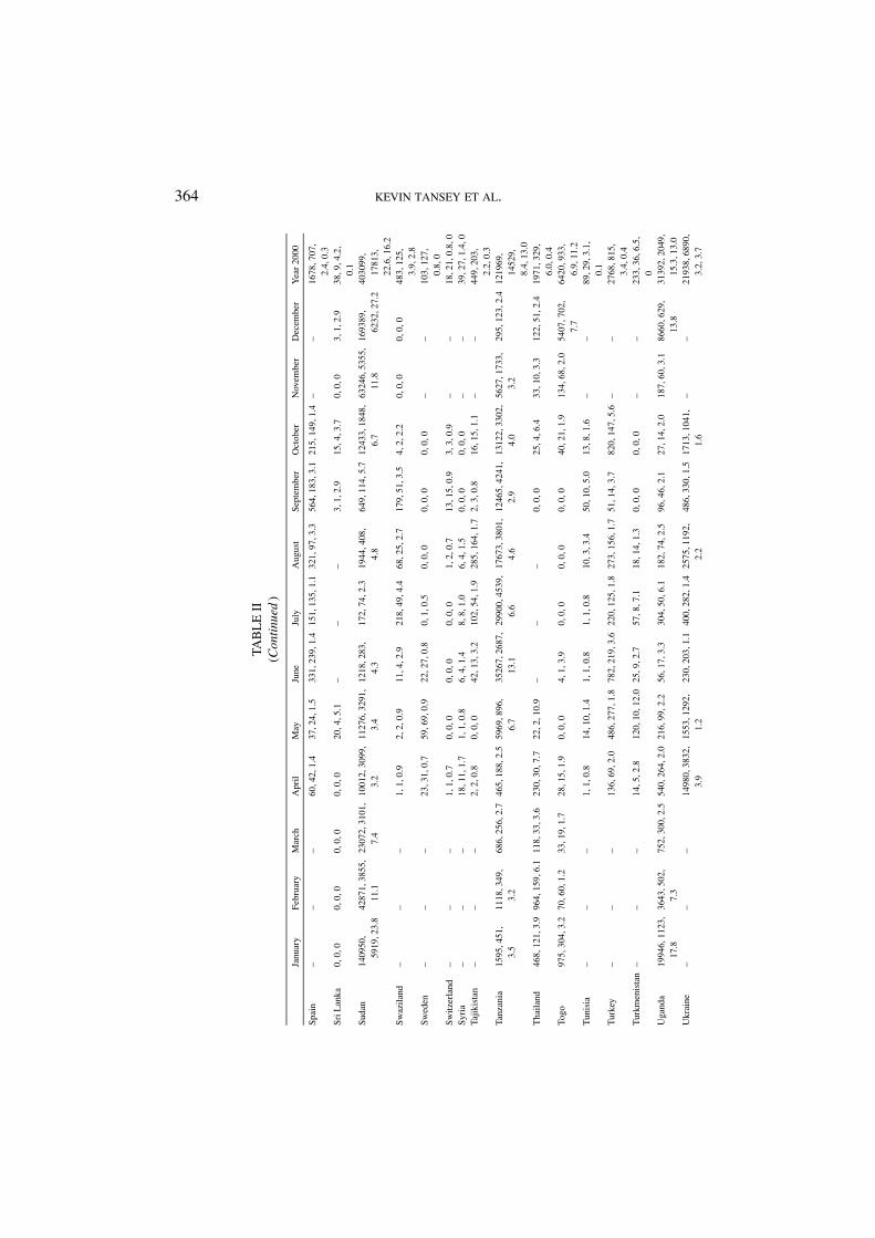
364 KEVIN TANSEY ET AL.
TAB
LE
II(C
onti
nued
)
Janu
ary
Febr
uary
Mar
chA
pril
May
June
July
Aug
ust
Sept
embe
rO
ctob
erN
ovem
ber
Dec
embe
rY
ear
2000
Spai
n–
––
60,4
2,1.
437
,24,
1.5
331,
239,
1.4
151,
135,
1.1
321,
97,3
.356
4,18
3,3.
121
5,14
9,1.
4–
–16
78,7
07,
2.4,
0.3
SriL
anka
0,0,
00,
0,0
0,0,
00,
0,0
20,4
,5.1
––
–3,
1,2.
915
,4,3
.70,
0,0
3,1,
2.9
38,9
,4.2
,0.
1Su
dan
1409
50,
5919
,23.
842
871,
3855
,11
.123
072,
3101
,7.
410
012,
3099
,3.
211
276,
3291
,3.
412
18,2
83,
4.3
172,
74,2
.319
44,4
08,
4.8
649,
114,
5.7
1243
3,18
48,
6.7
6324
6,53
55,
11.8
1693
89,
6232
,27.
240
3099
,17
813,
22.6
,16.
2Sw
azila
nd–
––
1,1,
0.9
2,2,
0.9
11,4
,2.9
218,
49,4
.468
,25,
2.7
179,
51,3
.54,
2,2.
20,
0,0
0,0,
048
3,12
5,3.
9,2.
8Sw
eden
––
–23
,31,
0.7
59,6
9,0.
922
,27,
0.8
0,1,
0.5
0,0,
00,
0,0
0,0,
0–
–10
3,12
7,0.
8,0
Switz
erla
nd–
––
1,1,
0.7
0,0,
00,
0,0
0,0,
01,
2,0.
713
,15,
0.9
3,3,
0.9
––
18,2
1,0.
8,0
Syri
a–
––
18,1
1,1.
71,
1,0.
86,
4,1.
48,
8,1.
06,
4,1.
50,
0,0
0,0,
0–
–39
,27,
1.4,
0Ta
jikis
tan
––
–2,
2,0.
80,
0,0
42,1
3,3.
210
2,54
,1.9
285,
164,
1.7
2,3,
0.8
16,1
5,1.
1–
–44
9,20
3,2.
2,0.
3Ta
nzan
ia15
95,4
51,
3.5
1118
,349
,3.
268
6,25
6,2.
746
5,18
8,2.
559
69,8
96,
6.7
3526
7,26
87,
13.1
2990
0,45
39,
6.6
1767
3,38
01,
4.6
1246
5,42
41,
2.9
1312
2,33
02,
4.0
5627
,173
3,3.
229
5,12
3,2.
412
1969
,14
529,
8.4,
13.0
Tha
iland
468,
121,
3.9
964,
159,
6.1
118,
33,3
.623
0,30
,7.7
22,2
,10.
9–
––
0,0,
025
,4,6
.433
,10,
3.3
122,
51,2
.419
71,3
29,
6.0,
0.4
Togo
975,
304,
3.2
70,6
0,1.
233
,19,
1.7
28,1
5,1.
90,
0,0
4,1,
3.9
0,0,
00,
0,0
0,0,
040
,21,
1.9
134,
68,2
.054
07,7
02,
7.7
6420
,933
,6.
9,11
.2T
unis
ia–
––
1,1,
0.8
14,1
0,1.
41,
1,0.
81,
1,0.
810
,3,3
.450
,10,
5.0
13,8
,1.6
––
89,2
9,3.
1,0.
1T
urke
y–
––
136,
69,2
.048
6,27
7,1.
878
2,21
9,3.
622
0,12
5,1.
827
3,15
6,1.
751
,14,
3.7
820,
147,
5.6
––
2768
,815
,3.
4,0.
4T
urkm
enis
tan
––
–14
,5,2
.812
0,10
,12.
025
,9,2
.757
,8,7
.118
,14,
1.3
0,0,
00,
0,0
––
233,
36,6
.5,
0U
gand
a19
946,
1123
,17
.836
43,5
02,
7.3
752,
300,
2.5
540,
264,
2.0
216,
99,2
.256
,17,
3.3
304,
50,6
.118
2,74
,2.5
96,4
6,2.
127
,14,
2.0
187,
60,3
.186
60,6
29,
13.8
3139
2,20
49,
15.3
,13.
0U
krai
ne–
––
1498
0,38
32,
3.9
1553
,129
2,1.
223
0,20
3,1.
140
0,28
2,1.
425
75,1
192,
2.2
486,
330,
1.5
1713
,104
1,1.
6–
–21
938,
6890
,3.
2,3.
7
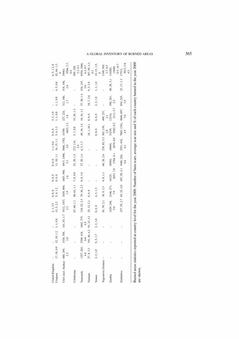
A GLOBAL INVENTORY OF BURNED AREAS 365U
nite
dK
ingd
om–
––
2,1,
2.5
0,0,
00,
0,0
0,0,
01,
1,0.
60,
0,0
3,3,
1.0
––
6,5,
1.2,
0U
rugu
ay17
,18,
0.9
12,1
0,1.
21,
1,0.
811
,5,2
.25,
4,1.
20,
0,0
11,1
0,1.
116
,15,
1.1
5,4,
1.3
1,1,
0.8
1,1,
0.8
4,5,
0.8
83,6
4,1.
3,0
USA
(inc
l.A
lask
a)68
8,29
5,2.
315
38,5
58,
2.8
141,
83,1
.735
12,1
553,
2.3
1839
,969
,1.
916
07,9
90,
1.6
4917
,149
6,3.
350
66,1
702,
3.0
1478
9,44
53,3
.322
7,22
4,1.
031
2,18
0,1.
751
8,19
6,2.
634
963,
9566
,3.7
,0.
4U
zbek
ista
n–
––
67,6
0,1.
168
,63,
1.1
7,8,
0.9
53,3
6,1.
527
2,11
4,2.
45,
7,0.
833
,26,
1.3
––
505,
238,
2.1,
0.1
Ven
ezue
la12
57,2
63,
4.8
2769
,418
,6.
618
42,3
75,
4.9
118,
52,2
.379
,36,
2.2
8,8,
1.0
27,2
0,1.
44,
3,1.
349
,34,
1.4
18,1
6,1.
127
,20,
1.4
434,
147,
3.0
6554
,106
6,6.
1,0.
7V
ietn
am27
,8,3
.319
1,46
,4.2
93,2
3,4.
125
,12,
2.1
0,0,
0–
––
10,1
,10.
10,
0,0
18,7
,2.6
9,3,
2.9
367,
85,4
.3,
0.1
Yem
en2,
2,1.
09,
5,1.
72,
2,1.
00,
0,0
4,3,
1.3
––
–0,
0,0
0,0,
02,
2,1.
01,
1,1.
019
,13,
1.5,
0Y
ugos
lavi
a(f
orm
er)
––
–81
,39,
2.1
30,9
,3.3
9,8,
1.1
68,2
6,2.
627
8,85
,3.3
383,
139,
2.8
499,
237,
2.1
––
1348
,505
,2.
7,0.
5Z
ambi
a–
––
1429
,248
,5.
821
46,2
71,
7.9
1412
5,20
31,7
.030
584,
3784
,8.1
1604
0,26
79,6
.033
239,
5382
,6.2
1211
4,21
11,5
.759
6,26
1,2.
388
,28,
3.1
1102
85,
1304
9,8.
5,14
.7Z
imba
bwe
––
–15
7,59
,2.7
65,3
2,2.
010
7,50
,2.1
1046
,226
,4.
625
51,4
18,
6.1
7865
,176
1,4.
548
46,6
97,
7.0
854,
245,
3.5
23,1
7,1.
317
513,
3013
,5.8
,4.
5
Bur
ned
area
sst
atis
tics
repo
rted
atco
untr
yle
velf
orth
eye
ar20
00.N
umbe
rof
burn
scar
s,av
erag
esc
arsi
zean
d%
ofea
chco
untr
ybu
rned
inth
eye
ar20
00ar
esh
own.
366 KEVIN TANSEY ET AL.
political boundary map as given in Table II. The column on the far right in Table IIdescribes the results of the annual synthesis. Topping the table of total burned areaper country in the year 2000 is Australia with 558,867 km2 that accounts for 7.3%of the total surface area of Australia with an average burned scar size of 28.4 km2.Three African countries, Sudan (403,099 km2), Angola (296,545 km2) and DRCongo (260,032 km2) follow Australia. Average scar size in these countries rangebetween 14.6 km2 and 22.6 km2. The total burned area in Russia was estimatedat 223,575 km2. However, what is interesting about the results for Russia (andalso for Kazakhstan) is that the average scar size, estimated at 3.4 km2 and 4.6 km2
respectively, is much smaller than is the case for many African nations and Australia.Also the total number of burn scars in Russia was very high with over 66,000individual scars being detected compared to between 7,500 and 23,000 for theother countries in the top 15 list. In the Central African Republic the number ofindividual burn scars detected is low compared to surrounding countries (7,592scars). However, the average size of a burn scar is second only to Australia at24.4 km2 resulting in a total burned area of 185,479 km2. After Russia, the nextfive countries with burned areas sorted into descending order are African nations(Central African Republic, Ethiopia, Tanzania, Zambia and Mozambique). For thewestern hemisphere countries, Argentina recorded the highest total burned areawith an average scar size of 3.3 km2 and quite a large number of individual scarsdetected (16,717 scars). The United States followed with an estimated 34,963 km2 ofburned areas, affecting approximately 0.4% of the total surface area of the country.Of particular interest is that the estimated burned area for Brazil (18,293 km2) in theyear 2000, came after the two countries named above and also Mexico (21,226 km2).In addition, the annual estimate for Canada is 5,687 km2 that is much lower thanthe 1989–1998 ten-year average of 33,580 km2 (Fraser et al., 2003). A discussionof the validity and relevance of these estimates and reasons for their derivation ispresented later in this paper. The countries in which vegetation burning has thegreatest influence on the land cover and has the largest impact on the people wholive there can be estimated by looking at the percentage of the total surface areaof the country that has been burned. Here we see that the table is dominated bythe African nations, occupying the top 15 places. At the top is the Central AfricanRepublic where 30% of the land surface is affected by burning, in position 15 isThe Gambia where 7.6% of the surface is burned.
The estimated global burned area for the year 2000 is just over 3.5 million km2.Because of different burning seasons the actual amount of biomass consumed byfire is higher than is reflected in the annual burned area total, because some regions(those located in the tropical Northern Hemisphere) were burned twice in the year2000. On a monthly basis, it was during the month of December 2000 that the great-est burned areas were detected comprising 523,496 km2 or 14.9% of the total an-nual burned area. Combined with the area estimated in January 2000, 438,715 km2
over 25% of the total annual burned area occurs during these two months. Thispeak in burning activity is associated with burning in the Northern Hemisphere

A GLOBAL INVENTORY OF BURNED AREAS 367
sub-tropical belt as well as in temperate regions of the Southern Hemisphere. An-other peak in activity, together accounting for 40% of global burned areas, occurs inthe months of June (9% of the global burned area), July (10.6%), August (9.6%) andSeptember (10.9%) that corresponds to burning activity in the temperate and borealzones in the Northern Hemisphere and also burning in the Southern Hemispheresub-tropical belt and in Australia.
4.2. A MONTH BY MONTH DESCRIPTION OF BURNING ACTIVITY IN THE YEAR 2000
In this section, all reported estimates of burnt areas (normally shown in brackets) arein square kilometers (km2). In January 2000, significant burning activity is detectedin the sub-Saharan region of Africa, concentrated in southern Sudan (140,950), Cen-tral African Republic (95,668), Ghana (9,776), Chad (13,457), Ethiopia (29,344),Kenya (9,745), northern Democratic Republic of the (DR) Congo (15,288), Nigeria(7,499) and northern Uganda (19,946). Burning activity is detected in the grass-land area of the Llanos of the Orinoco in Venezuela (1,257) and Colombia (2,068),the Pampas of central and southern Argentina (3,168) and, to a lesser extent inChile (348). Activity is also detected in Mexico (2,967) and southern states of theUS (688), the southern Indian peninsula (3,917), southern China located north ofVietnam (3,084), Burma (2191) and in Cambodia (755). Burning is widespread inAustralia (except for the tropical regions in the north) mainly down the east andwestern flanks (45,263).
February 2000 sees a reduction in burning activity in the sub-Saharan Africaregion. The activity has shifted southwards slightly but there are large regionsof burning activity remaining along the Sudan (42,871) and Ethiopian (19,906)border. Burning activity is still on-going in the grassland regions of Venezuela(2,769), Colombia (4,524), northern Brazil (566) and increasing in Mexico (3,193).Activity is increasing in Cambodia (3,006) and southern China (4,335). Activity inAustralia remains high with concentrations of activity detected in the non-tropicalnorthwest and west (27,515).
March 2000 sees, once again, a large number of burned scar detections inAustralia (16,924). The activity in India (12,937) peaks in March of the year 2000,whereas the activity has almost ceased in Thailand (118), Vietnam (93) and Laos(80). Activity in southern China (6,324) is increasing in area and becoming morewidespread. In sub-Saharan Africa activity is beginning to cease, with the onset ofthe wet season in May. However, some late season burning is still occurring, namelyin the southern Sudan (23,072) and Ethiopia (22,160). In Central America, burningis still detected in Mexico (1,864) however, now the burned scars are slightly largerand less numerous. Burning is on-going in the Llanos of the Orinoco covering bothVenezuela (1,842) Colombia (2,905), and also in central Argentina (2,468). Theburned areas detected during the months of January through to March 2000 areshown in blue in Figure 1 (bottom).

368 KEVIN TANSEY ET AL.
April is associated with the end of the Northern Hemisphere winter and the onsetof the Southern Hemisphere winter and consequent dry season. Burning activitythat can be described as being both widespread and intense is observed in the regionof southwest Russia (the total for Russia is 99,927), eastern Ukraine (14,980) andnorthern Kazakhstan (37,811) associated with agricultural land use in the region. Itis thought to be due to early season agricultural waste burning and further evidenceis seen on quick-look Landsat TM scenes. Burn scars are, in fact, detected all alongthis belt of steppe grassland and agriculture at around 50◦N (apart from desertand mountain areas) to eastern Mongolia (7,597), southern Russia, North Korea(1,057) and northern China (total for China is 19,084). Late season burning isstill occurring in India (9,549) and peaks in Burma (4,241) although the monsoonperiod is now only a few months away. April is the month of least burning activityin Australia (10,740). Burning activity is now diminishing rapidly in sub-SaharanAfrica during April. Fires occurring at these times, mainly in Ethiopia (11,470) andSudan (10,012), are really at the end of the dry season. The zone of fire activity hasnow shifted to the south with activity starting to pick up in Kenya (3,226). The leastamount of activity in the year 2000 is detected in the DR Congo during April (295).The beginnings of the Southern Hemisphere fire season seen in northern Angola(2,670), northern Zambia (1,429) and in the borderlands of Lesotho (337). In SouthAmerica, burning activity has all but ceased. Very few burn scars are being detectedin the Llanos of the Orinoco, and progressing further north, detections are nowrestricted to the south of Mexico (1,861) and also in Cuba (190). In North America(north of 30◦N), April is the onset of summer, the main season of burning activity.However, detections made during April (3,512 for the US and 20 for Canada) arerestricted to mainly agricultural regions, the main one being located in the Statesof Kansas and Oklahoma.
During May 2000, no significant detections are made in Canada (24). In theUS (1,840) activity is located mainly in northern California. Burning in Mexico(2,378) continues even into May indicating that the rains have not yet commenced.Burning activity is now detected in the coastal regions of Peru (1,944) and also inBolivia (787), now that the Southern Hemisphere dry season has started. Activityis now quite widespread and intense throughout Argentina (8,807) and Chile (421)between 28 and 38◦S. Burning activity is extremely intense in southern DR Congo(26,225), northern Angola (4,994), Kenya (7,283) and western Tanzania (5,969).Activity is still detected in southern Sudan (11,276) and Ethiopia (6,288). Furthersouth, burn scar detections are observed in Namibia (4,771), South Africa (2,542)and first observations are seen in southwest Madagascar (433). North of the Sahara,activity is detected at the delta of the Nile in Egypt (812). In May 2000, activityin western Europe was almost non-existent. Further east, activity is detected ineastern Ukraine (1,554), parts of Turkey (486), southern Russia (especially in thedelta region of the Volga River), and again at the border between Russia (total forRussia is 75,820) and Kazakhstan (6,668) but with less extent than in April. Isolatedscars are detected now further north in Russia. Burning activity in the region of
A GLOBAL INVENTORY OF BURNED AREAS 369
eastern Mongolia (13,688), southeastern Russia (as reported above) and northernChina (9,632) is now extremely intense. Extremely large and continuous burn scarsare observed in these areas. Burning activity has ceased in continental, southeastAsia but continues in India (8,917) just before the monsoon starts. In Australia(13,995), May is the beginning of the dry season in the north of the country andalready large burn scars are being detected in this region and also in the east of thecountry.
In June 2000, detection of activity in Australia is increasing (22,582) in the statesof the Northern Territory and northern Western Australia. Activity has ceased inIndia and southern China and has diminished and become isolated in northernChina (total for China is 6,449), Mongolia (2,845) and the Steppe regions of south-ern Russia. Activity in Russia (total for Russia is 16,005) is observed now in forestedareas with the onset of hot, dry and stable weather. Activity at the border betweenRussia and Kazakhstan (6,192) has reduced by a considerable amount. A consid-erable amount of activity is detected in central and southern Italy, Sicily, Sardinia(total for Italy is 1,289), Spain (331) and Portugal (91). The situation in Africa isthat burning has but almost ceased north of the equator and has become incrediblyintense and widespread throughout northern Angola (70,341), southern DR Congo(90,478), western Tanzania (35,267) and Zambia (14,125). Burn scars are also de-tected in the southwest corner of Botswana (10,106) and in South Africa (17,120).In Madagascar, burning activity is restricted to the dryer western half of the island(1,592). To the west across the Atlantic, burning activity is still continuing in cen-tral parts of northern Argentina (4,157) and is beginning in southern and easternregions of Brazil (1,721), specifically in the Mato Grosso and Goias districts, aswell as in parts of Bolivia (360). Burn scars are detected in the western states of theUS (1,607) in June 2000, but not on a large scale. The first detections are observedin Canada (254) and Alaska (included in the figure given above for the US). InFigure 1 (bottom), burned area detections made between April and June 2000 areshown in red.
In July 2000, burning activity in the forests of Canada (1,355) and Alaska(included in the figure for the US given below) and in the western states of the US(total for the US including Alaska is 4,917) are detected. In central and southernBrazil (2,910), Bolivia (2,196) and northern Argentina (7,653) burning activity isincreasing, but not at the scale seen in southern Africa. In Angola (112,482), almostall of the country is being affected by burning activity. The intensity of activity is alsobeing maintained in southern DR Congo (87,739), Zambia (30,584) and eastern andsouthern Tanzania (29,900). As well as moving south, the burning activity is alsoslowly progressing east. Large burn scars are now being detected in Mozambique(15,818) and eastern South Africa (9,516). In Zimbabwe there appears to be verylittle burning activity detected during the Southern Hemisphere dry season. Thepeak month of activity is detected in September (7,865) but compared with countriessurrounding Zimbabwe, the area burned is much smaller. In Madagascar (1,178)the burning activity is progressing further east. Burn scars are detected in Morocco
370 KEVIN TANSEY ET AL.
(375), Portugal (46), Spain (151) and southern Italy (108). Activity is detectedin southern Russia (the total for Russia is 7,897), near the border with Georgiaand in central Kazakhstan (4,248), northwest China (1,867) and southeast Russia(included in the total given above). Burn scars detected in Siberian forests arequite large and isolated. Isolated, small burn scars are detected on several islandsin Indonesia (77) and Malaysia (26). Activity in Australia (28,167) is detected inCape York, Northern Territory and northern and central parts of Western Australia.
August 2000 sees an increase in burning activity in Australia (69,616), especiallyin the north, but also in the southwest of the country. Detections are made in theIndonesian islands (513). In eastern Siberia (the total for Russia is 14,432), burningactivity is restricted to mainly forest fires that are quite large in size, but isolated.Large burn scars are observed in central Kazakhstan (16,836) and also further southin Kyrgyzstan (828) and Tajikistan (285) and in countries surrounding the Black Seaincluding Russia, Ukraine (2,575) and Bulgaria (763). Burning activity in westernEurope peaks in Portugal (369) and remains high in Spain (321) during August2000 and is observed in northern Algeria (377), southern Italy (191) and Greece(186). In southern Africa, the main region of burning activity is moving south andeast, but still remains intense throughout Angola (66,005), Zambia (16,040), Kenya(6,701), Tanzania (17,673), South Africa (10,109), Namibia (3,997) and Malawi(699). In Mozambique (32,812), burning activity is very intense and activity isstill increasing in Madagascar (1,775). Across the Atlantic, activity is increasingin central and southern Brazil (7,400) and in Paraguay (270). In North America,burn scars are continuing to be detected in western US including Alaska (5,066)and Canada (2,824).
In September 2000, the peak of the burning activity in North America is ob-served. Extensive burned areas are detected in the forest and woodland regions ofMontana, Idaho, Wyoming, Colorado, North Dakota and Minnesota (total for theUS including Alaska is 14,790). The peak month of burning activity in Canadaoccurred in August, with September’s value being much lower (1,207). September2000 also saw a diminishing of the burning activity in central and southern Brazil(2,500) and an increase of activity detected in northern Bolivia (3,516) and northernArgentina (5,559). The dry season in southern Africa is still very much in placeand the main region of burning activity still pushes further south and east. Activityin the west of southern Africa is located in the coastal regions of Angola (33,158)and further south in Botswana (6,003) and Namibia (12,745). Activity is detectedall along the eastern edge of southern Africa, from South Africa (19,752), throughMozambique (32,074), Zambia (33,239) and Tanzania (12,466) to Kenya (13,903)and Somalia (6,024). Activity peaks in Algeria (883) and Spain (564) and contin-ues in Italy (565), Greece (71) and Portugal (211) throughout September. Someburn scars are detected in eastern European countries such as Hungary (640) andRomania (770), southern Russia (the total for Russia is 3,186) and Kazakhstan(8,546) that could be due to the burning of agricultural land. In September 2000,the peak in burning activity is detected in the Indonesian islands (the total for all
A GLOBAL INVENTORY OF BURNED AREAS 371
islands is 916), the same being true for Papua New Guinea (96). The peak of burningactivity in Australia is observed in September 2000 (140,393). In Figure 1 (bottom),burn scars detected between July and September are shown in green.
The month of October 2000 is normally characterized by the onset of the dryseason (winter period) in the Northern Hemisphere tropical belt, associated withthe commencement of burning activities in the northern tropics and diminishingof activities in the southern tropics. In Australia, we are seeing more activity inthe center and south of the country (84,243). Detections are made in India (3,179),Nepal (957) and on the Tibetan Plateau in China (the total for China is 6,348). In thenortheast of China, activity has again increased possibly due to agricultural wasteburning or land clearance. Activity is detected in Russia (6,309), concentrated inthe border region with Kazakhstan (1,321) and also in North Korea (693). In sub-Saharan Africa, burning activity starts during October 2000 in southern Mauritania(8,515), Mali (3,747), northeast Nigeria (3,235), central Chad (19,484) and in re-gions of Sudan (12,433) and Ethiopia (4,124) in a line running at approximately15◦N of the equator. In southern Africa, the burning activity is generally dimin-ishing. However, regions of intense burning activity are still observed in centralBotswana (11,865), Zambia (12,114) and northern Mozambique (19,765). Activityin Madagascar (1,899) is now situated in towards the eastern side of the island. Areduction in burning activity is seen in northern Argentina (1,574), southern Brazil(2,294) and Bolivia (685). No activity is detected in October in the Llanos of theOrinoco. Burning activity has commenced in Mexico (1,876) and has practicallyceased in North America.
In November 2000, burn scars are detected in Mexico (4,082) as the early dry sea-son progresses. In southern Argentina, at the beginning of the Southern Hemispheresummer, activity is being detected. In southern Africa the fire season is ending fastwith the onset of the wet season, a concentration of burning activity is still ob-served in the southwest corner of South Africa (7,824) and northern Madagascar(1,062). Burning activity north of the equator in Africa is really starting to domi-nate the landscape with detections made in Senegal (3,324), Mali (8,608), Ghana(4,398), Benin (1,769), northern Cameroon (6,676), southern Chad (18,046), north-ern Central African Republic (11,216), Ethiopia (8,765) and all across southernSudan (63,246). Further east, burning activity is detected in isolated regions acrosscentral India (2,922) and in southern China (1,561) and Laos (411). Burning isstill occurring at a very large scale in Australia (85,698), dominant in the State ofQueensland.
In December 2000, burning activity in Australia (13,732) diminishes as rainscome to the north of the country but still occurring on a smaller scale in the Stateof Western Australia. In Africa, north of the equator, burning activity is increasingrapidly, slowly pushing further south and now dominant in a belt between 5 and14◦N (with the exception of Sierra Leone, Liberia and parts of Somalia) and in-cluding Sudan (169,385), Ghana (42,073), Benin (9,943), Chad (23,950), Cameroon(33,316), the Central African Republic (99,095), Somalia (6,753), Togo (5,407),
372 KEVIN TANSEY ET AL.
Nigeria (11,399) and the Ivory Coast (18,615) that peak in December, Senegal(1,957), Mali (3,134), Ethiopia (29,341). In South America, burning activity is de-tected in Argentina (6,696) at approximately 36◦S and we observe the beginningsof burning activity in the Llanos of the Orinoco in Venezuela (434) and Colombia(98). In Mexico (3,964), burning activity is observed with a large number of burnscars detected that are relatively small in area. Some burning is also detected in theState of Florida in the US (518). In Figure 1 (bottom), burn scars detected betweenOctober and December are shown in yellow-orange.
4.3. THE YEAR 2000 INVENTORY AS A REFERENCE DATASET
It has been shown in the literature that there is significant multi-annual variation inthe spatial distribution and also in the timing of vegetation fires. The causes of thesefluctuations are mainly driven by climatic factors such as temperature, precipitationand humidity. They may also be caused by changes in the management or use of theland. In the boreal regions, the inter-annual variation in burned area can be very largeindeed. It was well documented in the world’s media that in the summer of 1998,huge regions of forests were lost in Russia and Canada. In the literature, devastatingfires in Siberia, Mongolia and northern China during 1987 (Cahoon et al., 1994)have been described. Large scale climatic phenomena, such as El Nino and La Ninathat are disruptions of the ocean–atmosphere system in the tropical Pacific Ocean,can have a large impact on the severity and distribution of vegetation burning at aglobal scale. The 1997 El Nino year, characterised by a long dry season and elevatedtemperatures in the west Pacific resulted in devastating fires in Indonesia (Siegartet al., 2001) resulting in a huge release of carbon (0.81–2.57 gigatonnes) to theatmosphere (Page et al., 2002). The year 2000 was a La Nina year characterisedby unusually cool temperatures in the equatorial Pacific Ocean. This may be thereason why we observe a mild fire season in Brazil and Indonesia and a severe fireseason in the United States. The large inter-annual variability of carbon emissionscaused by biomass burning between 1997 and 2001 has also been demonstratedby Van der Werf et al. (2004), who revealed that negative global carbon monoxideanomalies occurred in the year 2000. To further highlight the potential annualvariability in burning activity, the frequency of active fires detected by the ATSR-2satellite acquired at night-time for the period 1997 to 2000 have been calculated. Thenumbers of fires detected were 133,970 (1997), 178,547 (1998), 120,650 (1999)and 116,478 (2000). These data show that in the year 2000, the least number of fireswere detected. It could therefore be assumed that the results presented in this paperreflect a lower than average estimate of burnt areas. The authors state that the burnedarea estimates should be used with caution if the user intends to describe generalconditions or make extrapolations for other years. Multi-annual estimates using thesame techniques are required for several years including years experiencing severalEl Nino and La Nina events.
A GLOBAL INVENTORY OF BURNED AREAS 373
4.4. VALIDATION ISSUES AND ERRORS IN THE GBA, 2000 INVENTORY
A global validation of the GBA, 2000 product is not available at this time. Neither isa figure for the overall accuracy of the burned area map at the global scale. Work iscurrently being undertaken to derive a benchmark dataset for the validation of globalscale thematic maps of biomass burning. The work is foreseen to be completed by theend of 2004 and will be published in refereed journals. Preliminary results have beenpresented at the recent CEOS Calibration/Validation Landcover Products Workshopin Boston and further work will be made presented at the 20th International Societyfor Photogrammetry and Remote Sensing Conference in Turkey in July 2004. Foreach of the regional algorithms a performance indicator is available, derived usingselected Landsat TM scenes over the corresponding region of interest. An outlineof the performance of the algorithms is given in Gregoire et al. (2003).
It is useful to indicate to the reader, regions where the authors believe there maybe some errors in the GBA, 2000 product, through either false detection’s or burnedareas that are not detected. Throughout the implementation of the regional burnedarea algorithms, care was taken to ensure that no large errors of commission or omis-sion were made. These checks were made using quick-look Landsat TM imageryavailable freely over the Internet, evidence of burning activity in the VGT productssuch as smoke and fire fronts, and evidence of burning activity documented in themedia. It is important to note that when the regional products were joined together,no major artifacts were observed at the join between regions. Artificial edge effects,however, are observed in central, southern Russia near to the Kazakhstan border.The artifacts are caused by the inherent properties of the IFI algorithm that calcu-lates the burned areas over a 200 km by 200 km window. An in-depth investigationwas made to understand the occurrence of these artifacts and they are believed to becaused by contamination of the image data (e.g. fire smoke, raw data processing)that is not masked out during the various data cleaning processes applied to thedata. These artifacts are only observed in the region of southern Russia and, giventhat the IFI algorithm is used extensively elsewhere with no further occurrencesreported, it was decided to accept these artifacts in the final product.
It is understood that there is a small underestimation of burned areas in Canadianforests and a commission error from falsely mapped fires of approximately 20%(Fraser et al., 2003). In the US, there may be some false detections in the semi-aridregions but this has not been confirmed. In parts of Mexico, due to complex landsurface properties, cloud cover and small burned areas, it is difficult to evaluatethe algorithms performance. For the whole of Central America, due to the samefactors mentioned above, the true burned area has probably been underestimated. InBrazil, we understand that we are not detecting smaller burned areas and burningbeneath the forest canopy. In addition, due to strong phenological influences inthe east of Brazil, we believe that an underestimation of the true burned area ismade. Significant areas of shadow caused by topography from the Andes mountainrange may yield some false detections. Estimation of the true burned area in Europe
374 KEVIN TANSEY ET AL.
and northern Africa provides difficulties because of the often-small size of the fireevents and burn scar. It is believed, though it has not been proven, that over halfof the land area in a pixel needs to burn before being detected by the algorithms,although this may depend on the algorithm being used. In the sub-Sahara regionof Africa, small errors are present in the burned area products, these are mainlycaused by flooding of non-permanent water features and dark rocks in the east ofAfrica. Compared with the magnitude of burning in Africa, these false detectionsare insignificant. In southern Africa, fire occurrence at the start of the rainy seasonmay have been missed due to cloud cover. In central and eastern Russia and northernAsia, it is understood that there are small areas of falsely detected burn scars inforested ecosystems and a small amount of omitted pixels in grassland ecosystems.A number of burned areas in insular southeast Asia are not detected, caused mainlyby excessive cloud coverage, a limited number of good observations of the groundsurface and, in common with the Amazon, many of burned areas being too smallto detect. In Australia, it is understood that the GBA, 2000 product underestimatesthe true burnt area. However, certain types of burning activity in Australia, forexample occurring in sparse, hummock Spinifex grasslands growing in bright, redsand soils (Graetz, personal communication, 2002) cause the surface to increase inreflectance. The GBA, 2000 algorithms mainly look for a drop in reflectance.
5. Conclusions
An inventory of the extent of burned vegetation for the year 2000 is described in thispaper, with reference to the seasonality and timing of burning activity on a monthlybasis and tabulated estimates of burned areas per country at global extent. The globalburned area products are available to the user community, free of charge through theInternet at the following website (http://www.gvm.jrc.it/fire/gba2000/index.htm).An accuracy assessment of the GBA, 2000 product is currently underway. Themethodology developed by the GBA, 2000 initiative will be used in the implemen-tation of the GlobCarbon project of the European Space Agency, providing global,monthly, burned area products over 5 years (1999–2003) from SPOT VGT data.
References
Andreae, M. O. and Merlet, P.: 2001, ‘Emission of trace gases and aerosols from biomass burning’,Global Biogeochem. Cycles 15, 955–966.
Barbosa, P. M., Gregoire, J.-M., and Pereira, J. M. C.: 1999a, ‘An algorithm for extracting burned areasfrom time series of AVHRR GAC data applied at a continental scale’, Remote Sensing Environ.69, 253–263.
Barbosa, P. M., Stroppiana, D., Gregoire, J.-M., and Pereira, J. M. C.: 1999b, ‘An assessment ofvegetation fire in Africa (1981–1991): Burned areas, burned biomass, and atmospheric emissions’,Global Biogeochem. Cycles 13, 933–950.
Boschetti, L., Flasse, S., Trigg, S., and de Dixmude, A. J.: 2002, ‘A multitemporal change detectionalgorithm for the monitoring of burnt areas with spot vegetation data’, in Bruzzone, L. and Smits,
A GLOBAL INVENTORY OF BURNED AREAS 375
P. (eds.), Analysis of MultiTemporal Remote Sensing Images, World Scientific, Singapore, pp.75–82.
Breiman, L., Friedman, J. H., Olshen, R. A., and Stone, C. J.: 1984, Classification and RegressionTrees, Wadsworth & Brooks, California.
Brivio, P. A., Maggi, M., Binaghi, E., Gallo, I., and Gregoire, J.-M.: 2002, ‘Exploiting spatial and tem-poral information for extracting burned areas from time series of SPOT-VGT data’, in Bruzzone,L. and Smits, P. (eds.), Analysis of MultiTemporal Remote Sensing Images, World Scientific,Singapore, pp. 132–139.
Cahoon Jr., D. R., Stocks, B. J., Levine, J. S., Cofer III, W. R., and Pierson, J. M.: 1994, ‘Satelliteanalysis of the severe 1987 forest fires in northern China and southeastern Siberia’, J. Geophys.Res. 99, 627–638.
Colby, J. D.: 1991, ‘Topographic normalization in rugged terrain’, Photogramm. Eng. Remote Sensing57, 531–537.
Conard, S. G., Sukhinin, A. I., Stocks, B. J., Cahoon, D. R., Davidenko, E. P., and Ivanova, G. A.:2002, ‘Determining effects of area burned and fire severity on carbon cycling and emissions inSiberia’, Climate Change 55, 197–211.
Dwyer, E., Pereira, J. M. C., Gregoire, J.-M., and DaCamara, C. C.: 1999, ‘Characterization of thespatio-temporal patterns of global fire activity using satellite imagery for the period April 1992to March 1993’, J. Biogeogr. 27, 57–69.
Eastwood, J. A., Plummer, S. E., Wyatt, B. K., and Stocks, B. J.: 1998, ‘The potential of SPOT-vegetation data for fire scar detection in boreal forests’, Int. J. Remote Sensing 19, 3,681–3,687.
Ershov, D. V. and Novik, V. P.: 2001, ‘Mapping burned areas in Russia with SPOT4 VEGETATION(S1 Product) imagery’, Final Report for the Joint Research Centre of the European Commission,contract number: 18176-2001-07-F1EI ISP RU.
Eva, H. D., Malingreau, J. P., Gregoire, J.-M., Belward, A. S., and Mutlow, C. T.: 1998, ‘The advanceof burnt areas in Central Africa as detected by ERS-1 ATSR-1’, Int. J. Remote Sensing 19, 1,635–1,637.
Fernandez, A., Illera, P., and Casanova, J. L.: 1997, ‘Automatic mapping of surfaces affected by forestfires in Spain using AVHRR NDVI composite data’, Remote Sensing Environ. 60, 153–162.
Fraser, R. H., Fernandes, R., and Latifovic, R.: 2003, ‘Multi-temporal mapping of burned forest overCanada using satellite-based change metrics’, Geocarto Int. 18, 37–48.
Fraser, R. H., Li, Z., and Cihlar, J.: 2000, ‘Hotspot and NDVI differencing synergy (HANDS): A newtechnique for burned area mapping over boreal forest’, Remote Sensing Environ. 74, 362–376.
Gregoire, J.-M., Tansey, K., and Silva, J. M. N.: 2003, ‘The GBA, 2000 initiative: Developing aglobal burned area database from SPOT-VEGETATION imagery’, Int. J. Remote Sensing 24,1,369–1,376.
Hansen, M. C., Defries, R. S., Townshend, J. R. G., and Sohlberg, R.: 2000, ‘Global land coverclassification at 1 km spatial resolution using a classification tree approach’, Int. J. Remote Sensing21, 1,331–1,364.
Hastings, D. A. and Dunbar, P. K.: 1998, ‘Development and assessment of the global land one-kmbase elevation digital elevation model (GLOBE)’, Int. Soc. Photogramm. Remote Sensing Arch.32, 218–221.
Houghton, R. A.: 1991, ‘Biomass burning from the perspective of the global carbon cycle’, in Levine,J. S. (ed.), Global Biomass Burning: Atmospheric, Climatic, and Biospheric Implications, MITPress, Cambridge, MA, pp. 321–325.
Isaev, A. S., Korovin, G. N., Bartalev, S. A., Ershov, D. V., Janetos, A., Kasischke, E. S., Shugart,H. H., French, N. H. F., Orlick, B. E., and Murphy, T. L.: 2002, ‘Using remote sensing to assessRussian forest fire carbon emissions’, Climate Change 55, 235–249.
Johnson, R. A. and Wichern, D. W.: 1988, Applied Multivariate Statistical Analysis (Second Edition),Prentice Hall, New Jersey.

376 KEVIN TANSEY ET AL.
Kasischke, E. S., Christensen, N. L., and Stock, B. J.: 1995, ‘Fire, global warming, and the carbonbalance of boreal forests’, Ecol. Appl. 5, 437–451.
Kempeneers, P., Swinnen, E., and Fierens, F.: 2002, GLOBSCAR Final Report, TAP/N7904/FF/FR-001 Version 1.2, VITO, Belgium.
Levine, J. S.: 1996, ‘FireSat and the global monitoring of biomass burning’, in Levine, J. S. (ed.),Biomass Burning and Global Change, The MIT Press, Cambridge, MA, pp. 107–132.
Malingreau, J. P. and Gregoire, J.-M.: 1996, ‘Developing a global vegetation fire monitoring systemfor global change studies: A framework’, in Levine, J. S. (ed.), Biomass Burning and GlobalChange, The MIT Press, Cambridge, MA, pp. 14–24.
Page, S. E., Siegart, F., Rieley, J. O., Boehm, H.-D. V., Jaya, A., and Limin, S.: 2002, ‘Theamount of carbon released from peat and forest fires in Indonesia during 1997’, Nature 420, 61–65.
Pereira, J. M. C.: 1999, ‘A comparative evaluation of NOAA/AVHRR vegetation indices for burnedsurface detection and mapping’, IEEE Trans. Geosci. Remote Sensing 37, 217–226.
Pereira, J. M. C., Mota, B. W., Privette, J. L., Caylor, K. K., Silva, J. M. N., Sa, A. C. L., and Ni-Meister,W.: in press, ‘A simulation analysis of the detectability of understory burns in Miombo Woodland’,Remote Sensing Environ.
Pereira, J. M. C., Pereira, B. S., Barbosa, P. M., Stroppiana, D., Vasconcelos, M. J. P., and Gregoire,J.-M.: 1999, ‘Satellite monitoring of fire in the EXPRESSO study area during the 1996 dryseason experiment: Active fires, burnt area and atmospheric emissions’, J. Geophys. Res. 104,30,701–30,712.
Roujean, J. L., Leroy, M., and Deschamps, P. Y.: 1992, ‘A bi-directional reflectance model of theearth’s surface for the correction of remotely sensed data’, J. Geophys. Res. 97, 20,455–20,468.
Roy, D., Lewis, P. E., and Justice, C. O.: 2002, ‘Burned area mapping using multi-temporal moderatespatial resolution data—A bi-directional reflectance model-based expectation approach’, RemoteSensing Environ. 83, 263–286.
Scholes, R. J., Kendall, J., and Justice, C. O.: 1996, ‘The quantity of biomass burned in SouthernAfrica’, J. Geophys. Res. 101, 23,667–23,676.
Schultz, M. G.: 2002, ‘On the use of ATSR fire count data to estimate the seasonal and interannualvariability of fire emissions’, Atmos. Chem. Phys. Discuss. 2, 1,159–1,179.
Siegart, F., Ruecker, G., Hinrichs, A., and Hoffmann, A. A.: 2001, ‘Increased damage from fires inlogged forests during droughts caused by El Nino’, Nature 414, 437–440.
Silva, J. M. N., Pereira, J. M. C., Cabral, A. I., Sa, A. C. L., Vasconcelos, M. J. P., Mota, B., andGregoire, J.-M.: 2003, ‘The area burned in Southern Africa during the 2000 dry season’, J.Geophys. Res. 108, D13, 8498, doi: 10.1029/2002JD002320.
Silva, J. M. N., Sousa, A. M. O., Pereira, J. M. C., Tansey, K., and Gregoire, J.-M.: 2002, ‘A Contri-bution for a Global Burned Area Map’, in Viegas, D. X. (ed.), Forest Fire Research & WildlandFire Safety, Millpress, Rotterdam.
Stroppiana, D., Pinnock, S., Pereira, J. M. C., and Gregoire, J. M.: 2002, ‘Radiometric analysis ofspot vegetation images for burnt area detection in Northern Australia’, Remote Sensing Environ.82, 21–37.
Stroppiana, D., Tansey, K., Gregoire, J.-M., and Pereira, J. M. C.: 2003, ‘An algorithm for mappingburnt areas in Australia using SPOT-VEGETATION data’, IEEE Trans. Geosci. Remote Sensing41, 907–909, doi: 10.1109/TGRS.2003.808898.
Tansey, K.: 2002, Implementation of the Regional Burnt Area Algorithms for the GBA, 2000 Initiative,Publication of the European Communities, EUR 20532 EN.
Tansey, K., Gregoire, J. M., Stroppiana, S., Sousa, A., Silva, J. M. N., Pereira, J. M. C., Boschetti,L., Maggi, M., Brivio, P. A., Fraser, R., Flasse, S., Ershov, D., Binaghi, E., Graetz, D., andPeduzzi, P.: 2004, ‘Vegetation burning in the year 2000: Global burned area estimates from SPOTVEGETATION data’, J. Geophys. Res. 109, D14503 doi: 10.1029/2003JD003598.
A GLOBAL INVENTORY OF BURNED AREAS 377
Trigg, S. and Flasse, S.: 2000, ‘Characterizing the spectral-temporal response of burned savannahusing in situ spectroradiometry and infrared thermometry’, Int. J. Remote Sensing 21, 3,161–3,168.
Van Aardenne, J. A., Dentener, F. J., Olivier, J. G. J., Klein Goldewijk, C. G. M., and Lelieveld, J.:2001, ‘A 1◦ × 1◦ resolution data set of historical anthropogenic trace gas emissions for the period1890–1990’, Global Biogeochem. Cycles 15, 909–928.
Van der Werf, G. R., Randerson, J. T., Collatz, G. J., Giglio, L., Kasibhatla, P. S., Avelino, A., Olsen,S. C., and Kasischke, E. S.: 2004, ‘Continental-scale partitioning of fire emissions during the1997–2001 El Nino/La Nina period’, Science 303, 73–76.
Wotawa, G., Novelli, P. C., Trainer, M., and Granier, C.: 2001, ‘Inter-annual variability of summertimeCO concentrations in the Northern Hemisphere explained by boreal forest fires in North Americaand Russia’, Geophys. Res. Lett. 28, 4,575–4,578.
(Received 13 May 2003; in revised form 14 June 2004)