（1）

A Gentle Introduction to Isogeometric AnalysisPart 2: NURBS Curve & Surface *

Keiji YANASE **

In a previous study, we studied some features of the B-spline basis function. One of the applications of basis function is the representation of geometrical shape. In the present paper, based on the B-spline basis function, NURBS basis function for curve and surface is introduced. Then, the description of geometry using NURBS is discussed through several examples. Further, by taking advantage of MATLAB software, the data structure for geometrical representation is also studied. It is demonstrated that, by taking advantage of NURBS, an efficient and accurate geometry description can be achieved with a small number of parameters.

Key Words : NURBS, Curve, Surface, NURBS toolbox, MATLAB

1. NURBS Basis Functions　B-splines are highly advantageous, as they can be applied to control the continuity and span of a function. However, further improvements are still possible. In fact, the shape of curve can be further controlled by using the weight.　Based on the B-spline basis function, , NURBS basis function, , is rendered as [1][2]:

　　　　　　　 (1)

To retain the partition of unity condition, a division of the sum of the B-splines multiplied by the weights is required. Thus,

(2)

Further, is no longer a polynomial, but a rational function (i.e., both the numerator and the denominator are polynomials). Therefore, the function presented in Eq. (2) is called non-uniform rational B-splines or NURBS.　Use of Eq. (2) in conjunction with the control point coordinates, Pi, leads to an equation for a NURBS curve:

　　　　　　　　　 (3)

In Eq. (3), the control points can be chosen independently from their associated weights. It is also noteworthy that, if all weights are equal, it follows that and the

*Manuscript received: April 24, 2017 **Department of Mechanical Engineering

curve is again a polynomial. Thus, B-spline is a special case of NURBS.　Here, let us consider the following knot vector for quadratic B-spline function (i.e., p = 2):

(4)

In Eq. (4), the maximum knot index is 7 and with . Accordingly, the number of basis functions, n, is 4. The

B-spline basis functions are thus rendered as [3]:

　　 (5)

　　 (6)

　　 (7)

　　 (8)

Consequently, based on Eq. (1), NURBS basis functions are obtained as:

　　　 (9)

　　　 (10)

　　　 (11)

　　　 (12)

− 1−

（2）

福岡大学工学集報　第99号（平成29年9月）

　In order to demonstrate the effect of the weights, the basis functions and the corresponding curves are shown in Figs. 1 and 2, respectively. It can be seen that a higher order value of weight (w3 = 2) shifts the curve toward the 3rd control point. This additional flexibility makes the NURBS so attractive for describing geometry.　MATLAB [4] is a higher-level programming language that is suitable for quick implementation of concepts and generation of graphical output. In this work, we also make use of the NURBS toolbox available in MATLAB. Though familiarity with the toolbox is required to ensure correct input, it is efficiently programmed and bug free [1]. A detailed MATLAB code for generating graphs shown in Fig. 2 is provided below. This program can be executed with MATLAB 2016b.__________________________________________________

− 2−

（3）

A Gentle Introduction to Isogeometric Analysis Part 2: NURBS Curve & Surface（YANASE）

__________________________________________________

　An alternative code that utilizes the NURBS toolbox is shown below. Obviously, an efficient calculation can be performed with a few lines of code. The NURBS toolbox is provided as one of MATLAB add-ons and it can be easily installed by clicking an icon in the menu.

__________________________________________________

__________________________________________________

It should be noted that the functions take homogeneous coordinates/parameters at the control points as input. As a result, they have to be multiplied by the coresponding weights before being supplied to the function. Namely, we need to set the coordinates of control points as follows:

(13)

2. Representing Curves with NURBS2.1. Circular Arc　For a better understanding of the concepts discussed thus far, let us examine an algorithm for plotting the circular arc [1]. NURBS basis functions of order p = 2 can exactly represent a circular arc. Let us compute the control point coordinates and weights for a circular arc of radius r, start angle and end angle .

If the sustained angle is smaller than we can substitute and defi ne three control points, as shown in Fig. 3. Then, the knot vector is given as:

　　　　　　　　 (14)

It is noted that Eq. (14) is open knot vector with p+1 (= 3) multiplicity. The coordinates and weights of the control points are computed as follows:

(1) If the sustained angle is greater than we set and compute three control points by using

・・・・

・・・・

− 3−

（4）

福岡大学工学集報　第99号（平成29年9月）

Eqs. (15) − (17).(2) Then, we set & and compute two additional control points by using Eqs. (15) − (17). (3) Correspondingly, the knot vector is given as:

　　　　　　 (18)

(1) If the sustained angle exceeds but is smaller than we set and compute three control points

by using Eqs. (15) − (17). (2) In the next step, we set and compute two additional control points by using Eqs. (15) − (17). (3) Finally, we set and compute two additional control points by using Eqs. (15) − (17).(4) Correspondingly, the knot vector is given as:

　　　　 (19)

(1) If the sustained angle is greater than we set and compute three control points by using

Eqs. (15) − (17). (2) Then, we set and compute two additional control points by using Eqs. (15) − (17). (3) Further, we set and compute two additional control points by using Eqs. (15) − (17).(4) Finally, we set and compute two additional control points by using Eqs. (15) − (17).(5) Correspondingly, the knot vector is given as:

　　 (20)

To plot a circular arc, the following MATLAB code (subroutines) can be used. The function “Arcseg” [1] is executed to determine the three control point coordinates and weights based on Eqs. (15) − (17).

The function “Arc” [1] is executed in order to compute

the coordinates and weights by considering the sustained

angle (αe−αs ).

− 4−

（5）

A Gentle Introduction to Isogeometric Analysis Part 2: NURBS Curve & Surface（YANASE） − 5−

（6）

福岡大学工学集報　第99号（平成29年9月）

__________________________________________________

2.2. Plate with a Hole　This example demonstrates the ease with which continuity can be controlled with NURBS. A quarter of a plate with a circular arc is represented with NURBS, while the order of basis function, p, is set to 2 [1]. For this case, double entries in the knot vector at each corner node are required to ensure C0-continuity. The quarter plate with a hole, as shown in Fig. 5, is exactly represented through NURBS. The corresponding MATLAB code and the graphical representation of the results are provided below and in Fig. 5, respectively.__________________________________________________

3. Surfaces with NURBS　To represent the surfaces, two coordinates in the parameter space are utilized. This allows the NURBS basis functions to be computed using the following tensor product:

　　　　　　 (21)

Then, NURBS surface is rendered by the following equation:

　　　　　　　 (22)

Based on these function files, a circular arc can be drawn

using the following MATLAB code (r = 1, αs = 0, αe = 3π/4).

Some examples are shown in Fig. 4.

− 6−

（7）

A Gentle Introduction to Isogeometric Analysis Part 2: NURBS Curve & Surface（YANASE）

　The process of surface creat ion with NURBS is demonstrated using an example depicted in Fig. 6, which can be created without using NURBS toolbox. Although this program is rather crude, it helps in elucidating the essence of Eq.(22).

− 7−

（8）

福岡大学工学集報　第99号（平成29年9月）

　On the other hand, by using the NURBS toolbox, the surface can be created much more efficiently. However, proficiency in the use of structures and inputs for NURBS toolbox is required.

　In some cases, surfaces are created by revolving a curve (generatrix) around a rotational axis, as shown in Fig. 7. The following function file, “Surfrev” [1] can be used to create a surface based on revolution.

− 8−

（9）

A Gentle Introduction to Isogeometric Analysis Part 2: NURBS Curve & Surface（YANASE）

__________________________________________________

3.1. Cylindrical Surface

　A cylindrical surface [1], as shown in Fig. 8, is created by executing the following MATLAB code:

− 9−

（10）

福岡大学工学集報　第99号（平成29年9月）

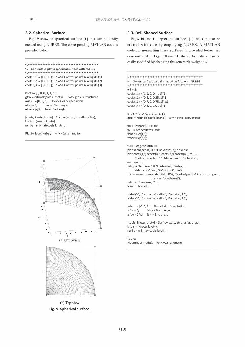
3.2. Spherical Surface　Fig. 9 shows a spherical surface [1] that can be easily created using NURBS. The corresponding MATLAB code is provided below:

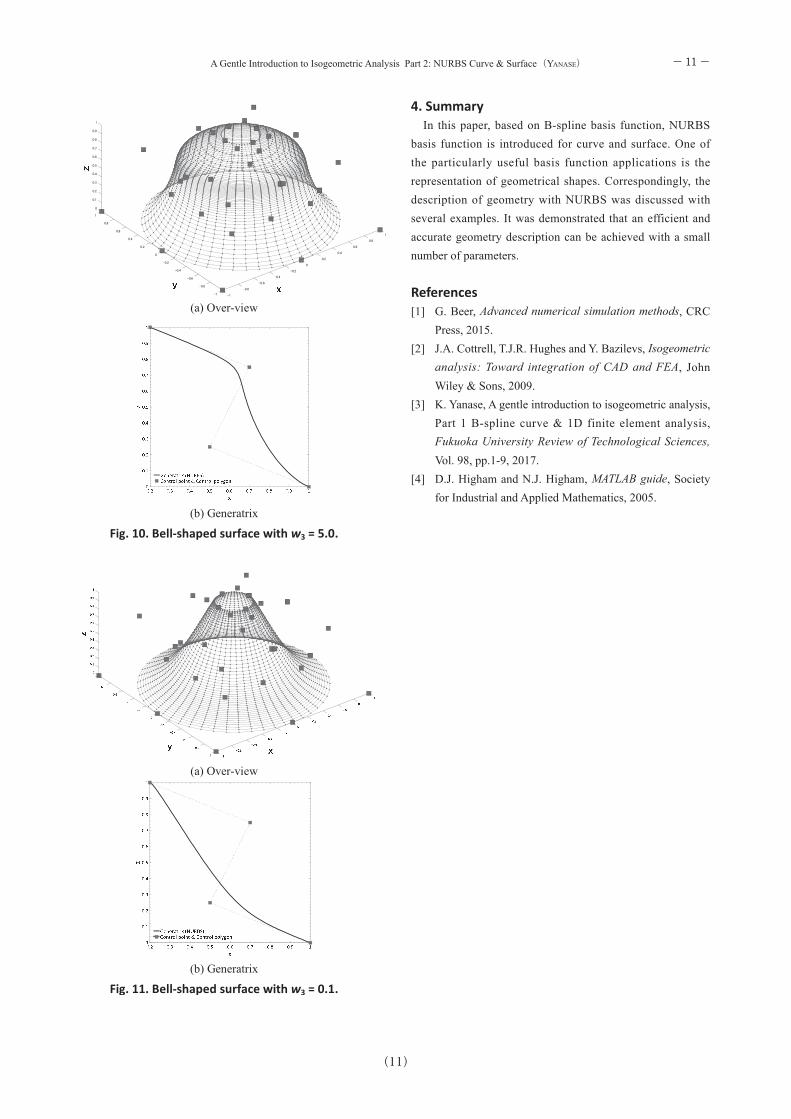
3.3. Bell-Shaped Surface　Figs. 10 and 11 depict the surfaces [1] that can also be created with ease by employing NURBS. A MATLAB code for generating these surfaces is provided below. As demonstrated in Figs. 10 and 11, the surface shape can be easily modified by changing the generatrix weight, w3.

− 10 −

（11）

A Gentle Introduction to Isogeometric Analysis Part 2: NURBS Curve & Surface（YANASE）

4. Summary　In this paper, based on B-spline basis function, NURBS basis function is introduced for curve and surface. One of the particularly useful basis function applications is the representation of geometrical shapes. Correspondingly, the description of geometry with NURBS was discussed with several examples. It was demonstrated that an efficient and accurate geometry description can be achieved with a small number of parameters.

References[1] G. Beer, Advanced numerical simulation methods, CRC

Press, 2015.[2] J.A. Cottrell, T.J.R. Hughes and Y. Bazilevs, Isogeometric

analysis: Toward integration of CAD and FEA, John Wiley & Sons, 2009.

[3] K. Yanase, A gentle introduction to isogeometric analysis, Part 1 B-spline curve & 1D finite element analysis, Fukuoka University Review of Technological Sciences, Vol. 98, pp.1-9, 2017.

[4] D.J. Higham and N.J. Higham, MATLAB guide, Society for Industrial and Applied Mathematics, 2005.

− 11 −