A generalized, bioclimatic index to predict foliar phenology in response to climate

A generalized, bioclimatic index to predict foliarphenology in response to climate

W I L L I AM M . J O L LY *, R AMAKR I SHNA NEMAN I w and S T E V EN W. RUNN ING *

*NTSG, College of Forestry and Conservation, SC428, University of Montana, Missoula, MT 59812, USA,

wNASA AMES Research Center, Moffett Field, CA 94035, USA

Abstract

The phenological state of vegetation significantly affects exchanges of heat, mass, and

momentum between the Earth’s surface and the atmosphere. Although current patterns

can be estimated from satellites, we lack the ability to predict future trends in response

to climate change. We searched the literature for a common set of variables that might be

combined into an index to quantify the greenness of vegetation throughout the year. We

selected as variables: daylength (photoperiod), evaporative demand (vapor pressure

deficit), and suboptimal (minimum) temperatures. For each variable we set threshold

limits, within which the relative phenological performance of the vegetation was

assumed to vary from inactive (0) to unconstrained (1). A combined Growing Season

Index (GSI) was derived as the product of the three indices. Ten-day mean GSI values for

nine widely dispersed ecosystems showed good agreement (r40.8) with the satellite-

derived Normalized Difference Vegetation Index (NDVI). We also tested the model at a

temperate deciduous forest by comparing model estimates with average field observa-

tions of leaf flush and leaf coloration. The mean absolute error of predictions at this site

was 3 days for average leaf flush dates and 2 days for leaf coloration dates. Finally, we

used this model to produce a global map that distinguishes major differences in regional

phenological controls. The model appears sufficiently robust to reconstruct historical

variation as well as to forecast future phenological responses to changing climatic

conditions.

Keywords: climate change, global, minimum temperature, model, phenology, photoperiod, vapor

pressure deficit

Received 23 June 2004 and accepted 4 November 2004

Introduction

For centuries, people have observed annual variation in

the dates at which buds break and flowers bloom

(Sparks & Carey, 1995). The science of plant phenology

is concerned with understanding the variability of these

reproductive and vegetative cycles, particularly in

relation to their biotic and abiotic forcings (Lieth,

1974). Plant vegetative cycles, such as the timing and

duration of foliage, determine exchange periods of

carbon dioxide and water between the Earth’s surface

and the atmosphere. Recent decades have seen changes

in the timing and duration of plant greenness across

much of the globe (Myneni et al., 1997; Menzel &

Fabian, 1999; Schwartz & Reiter, 2000; Matsumoto et al.,

2003) and these changes could have a large impact on

the global carbon cycle (Keeling et al., 1996).

Satellite observations, ground observations, and

mathematical models are all key components that aid

in the study of large-scale phenological patterns

(Schwartz, 1999). Researchers have used satellite data

to adequately map the waxing and waning of vegeta-

tion greenness across the Earth’s surface (Justice et al.,

1985). These phenological estimates have improved

regional and interannual predictions from general

circulation models (Chase et al., 1996), but such coupled

land–atmosphere models often use fixed vegetation

phenology parameters (Sellers et al., 1996). This neglects

the dynamic characteristics of surface vegetation.

Ground observations aid in developing a more

dynamic link between driving variables, such as

climate, and phenophase transitions, but these observa-

tions are generally not well distributed globally and the

quality of such data is dependent on the skills of the

observer (Menzel, 2002). Mathematical models bridgeCorrespondence: William M. Jolly, tel. 1 1 (406) 243 6230,

fax 1 1 (406) 243 4510, e-mail: [email protected]

Global Change Biology (2005) 11, 619–632, doi: 10.1111/j.1365-2486.2005.00930.x

r 2005 Blackwell Publishing Ltd 619

the gap between the extensive spatial scales available

from satellite-derived observations and the linkage to

driving variables that can potentially be derived from

ground observations. Work has been carried out to

combine such phenology models as part of land-surface

models that are then coupled with global climate

models to provide dynamic, large-scale predictions of

interactions between vegetation and climate, but this

work would benefit from a more generalized and

complete description of vegetation phenology (Foley

et al., 1998).

Phenology models predict canopy greenness from

climate data because climate is the primary driver at

large scales (Botta et al., 2000). In the mid- and high

latitudes, phenology is controlled by temperature and

photoperiod (Myneni et al., 1997; White et al., 1997;

Chuine & Cour, 1999; Jarvis & Linder, 2000; Schwartz

& Reiter, 2000), but regionally, water limitations may

also be important (Penuelas et al., 2004). In the tropics,

phenology is controlled either by seasonal rainfall

(Childes, 1989; de Bie et al., 1998; Bach, 2002) or

photoperiod (Njoku, 1958; Borchert & Rivera, 2001).

However, single climatic factors do not always limit

phenology at a given location; sometimes multiple

factors control phenology concurrently or at different

times of the year (Nilsen & Muller, 1981; White et al.,

1997; Jame et al., 1998).

Foliar phenology models have been developed to

predict dates of leaf flushing and leaf senescence from

available climate data (Kramer, 1994; White, 1997 #19;

Botta et al., 2000; Kang et al., 2003; Jolly & Running,

2004), but many of these models were developed for

temperate ecosystems where phenophase transitions

are easily defined. In the tropics, seasonal water

availability promotes rapid leaf flushing while leaf

senescence may occur gradually over as much as 6

months (Childes, 1989); any choice of a single-leaf

senescence date would be arbitrary at best.

Attempts to model phenology globally have been

constrained to the prediction of the start of leaf

flushing, or onset, and have neglected the dynamics

of leaf fall at the end of the growing season (Botta et al.,

2000). In addition, continental or larger scale phenol-

ogy models require a priori knowledge of the climate

or vegetation in order to discretely switch among

biome-specific models (White et al., 1997; Botta et al.,

2000). This limits their utility for forecasting the

impacts of climate change on vegetation because the

limiting factor at a given location may change. An

alternative to traditional phenology models might be

to continuously characterize within-year variation in

canopy leaf area, rather than finite phenophase

transitions, by combining the limitations and interac-

tions of all key climate variables into a single index of

foliar phenology. This is possible if we assume that

there are a minimum set of requirements that must be

met for a plant to either initiate or maintain a certain

phenological state.

In this paper, we seek to develop a simple, general-

ized phenology model to test the hypothesis that there

is such a set of common climatic conditions that

interact to limit foliar phenology globally. We are

interested in predicting not only the beginning and

end of the growing season but also the status of the

canopy throughout the year without a priori knowl-

edge of the vegetation or climate. We show that the

model can also predict phenophase transition dates

like traditional foliar phenology models. We seek to

drive the model with readily available climatic data,

and to provide an integrative index that combines the

weighed effects of daylength (photoperiod), evapora-

tive demand (vapor pressure deficit (VPD)), and

suboptimal (minimum) temperature. We test the

generality of the model at widely diverse locations

and judge its performance against satellite-derived

estimates of the Normalized Difference Vegetation

Index (NDVI). We also test the model at a temperate

deciduous forest site to assess its ability to predict

interannual differences in leaf flush and leaf senes-

cence dates.

Methods

Model development

We searched for a common set of meteorological

variables that together might account for much of the

variation observed in the seasonal phenology recorded

across the Earth. We chose three that are readily

available and good surrogates for the underlying

mechanisms: low temperatures, evaporative demand,

and photoperiod. From the literature, we extracted

threshold limits for each variable, between assuming

that phenological activity varied linearly from inactive

(0) to unconstrained (1). These functions and their

derivations are described in detail below. The product

of the three indices forms a combined model that is

calculated daily and integrated as a 21-day running

average to avoid reaction to short-term changes in

environmental conditions (Lieberman, 1982; Lecho-

wicz, 2001).

Minimum temperature. Many of the biochemical

processes of plants are sensitive to low temperatures

(Levitt, 1980). Although ambient air temperatures

certainly influence growth, constraints on phenology

appear to be more closely related to restrictions on

water uptake by roots when soil temperatures are

620 W. M . J O L LY et al.

r 2005 Blackwell Publishing Ltd, Global Change Biology, 11, 619–632

suboptimal (Waring, 1969). Many field studies show

variable ecosystem responses over a range of minimum

temperatures. Jarvis & Linder (2000) demonstrated that

northern spruces and pines increase their photo-

synthesis rapidly once temperatures exceed �1 1C.

Temperatures below freezing are lethal, however, for

tropical trees (Larcher, 1995). Temperatures below

�2 1C can freeze water in the xylem of some trees

(Zimmerman, 1964). Minimum temperature is also a

stronger indicator of climate change than either average

or maximum temperature (IPCC, 2001). To incorporate

a range of species, we chose a range encompassed by a

lower minimum temperature threshold of �2 1C

(TMMin) and an upper threshold of 5 1C (TMMax). A

similar range of low-temperature sensitivities has been

reported elsewhere (Larcher & Bauer, 1981).

A minimum temperature index (iTMin), presented

graphically in Fig. 1a, was created as follows:

iTMin ¼0; ifTMin � TMMin;TMin � TMMin

TMMax � TMMin; ifTMMax > TMin > TMMin;

1; ifTMin � TMMax;

8><>:

ð1Þ

where iTMin is the daily indicator for minimum

temperature and is bounded between 0 and 1 and

TMin is the observed daily minimum temperature in

degrees Celsius. For all tests, TMMin5�2 1C and

TMMax5 5 1C.

VPD. Water stress causes partial to complete stomatal

closure (Mott & Parkhurst, 1991), reduces leaf

development rate (Salah & Tardieu, 1996), induces the

shedding of leaves (Childes, 1989), and slows or halts

cell division (Granier & Tardieu, 1999). Although

models are available to calculate a soil water balance,

they require knowledge of rooting depth, soil texture,

latent heat losses, and precipitation. As a surrogate, we

selected an index of the evaporative demand, the VPD

of the atmosphere. At low values, latent heat losses are

unlikely to exceed available water, whereas at high

values, particularly if sustained, photosynthesis and

growth are likely to be significantly limited. The

distribution of vegetation with different phenological

patterns is thus, very sensitive to seasonal changes in

VPD (Huffaker, 1942).

From the literature, we find evidence that VPD less

than 900 Pa should exert little effect on stomata whereas

values greater than 4100Pa generally are sufficient to

force complete stomatal closure, even when the soils are

moist (Osonubi & Davies, 1980; Tenhunen et al., 1982).

Although these limits vary by locations and species

(White et al., 2000), we chose a common set of para-

meters for all sites. The VPD index (iVPD), shown

graphically in Fig. 1b, was, therefore, derived as

follows:

iVPD ¼0; ifVPD � VPDMax;

1� VPD� VPDMin

VPDMax � VPDMin; ifVPDMax > VPD > VPDMin;

1; ifVPD � VPDMin;

8><>:

ð2Þ

(a)

Tmin (°C)−4 −2 0 2 4 6

iTm

in

0.0

0.2

0.4

0.6

0.8

1.0

(b)

Vapor pressure deficit (Pa)0 1000 2000 3000 4000

i VP

D

0.0

0.2

0.4

0.6

0.8

1.0

(c)

Photoperiod (h)10.0 10.5 11.0 11.5

i Pho

to

0.0

0.2

0.4

0.6

0.8

1.0

Fig. 1 Graphic representation of minimum temperature, vapor

pressure deficit, and photoperiod indicator functions used to

predict foliar phenology. For each variable, threshold limits are

defined, between which the relative constraint on phenology is

assumed to vary linearly from inactive (0) to unconstrained (1).

P R ED I C T I NG FO L I A R PHENOLOGY IN R E S PON S E TO CL IMAT E 621


where iVPD is the daily indicator for VPD and is

bounded between 0 and 1 and VPD is the observed

daily VPD in Pascals. For all tests, VPDMin5 900 Pa and

VPDMax5 4100Pa.

Photoperiod. Photoperiod provides a plant with a

reliable annual climatic cue because it does not vary

from year to year at a given location. We assume that

photoperiod provides the outer envelope within which

other climatic controls may dictate foliar development.

Studies have shown that photoperiod is important to

both leaf flush and leaf senescence throughout the

world (Njoku, 1958; Rosenthal & Camm, 1997; White

et al., 1997; Hakkinen et al., 1998; Partanen et al., 1998;

Borchert & Rivera, 2001). Photoperiod also interacts

with temperature to limit foliar phenology, rendering

temperature changes ineffective without corresponding

photoperiod changes (Partanen et al., 1998). We

assumed photoperiods of 10 h or less completely

limited canopy development and 11 h or more

allowed canopies to develop unconstrained. The

photoperiod index (iPhoto), shown graphically in Fig.

1c, was, therefore, derived as follows:

iPhoto ¼0; ifPhoto � PhotoMin;Photo� PhotoMin

PhotoMax � PhotoMin; ifPhotoMax > Photo > PhotoMin;

1; ifPhoto � PhotoMax;

8><>:

ð3Þ

where iPhoto is the daily photoperiod indicator and

Photo is the daily photoperiod in seconds. For all tests,

PhotoMin5 36 000 s (10 h) and PhotoMax5 39 600 s (11 h).

The Growing Season Index (GSI)

The product of the individual daily indicators for

minimum temperature, VPD, and photoperiod forms a

single metric which can be monitored for canopy

greenness, hereafter referred to as the GSI. The GSI is

a daily indicator of the relative constraints to foliar

canopy development or maintenance due to climatic

limits. It is continuous but bounded between 0

(inactive) and 1 (unconstrained). The daily metric (iGSI)

is calculated as follows:

iGSI ¼ iTmin � iVPD� iPhoto; ð4Þ

where iGSI is the daily GSI, iTmin is the minimum

temperature indicator, iVPD is the VPD indicator, and

iPhoto is the photoperiod indicator. The daily GSI is

then calculated as the 21-day moving average of daily

indicator, iGSI, for all sites. The moving average serves

to buffer single extreme events from prematurely

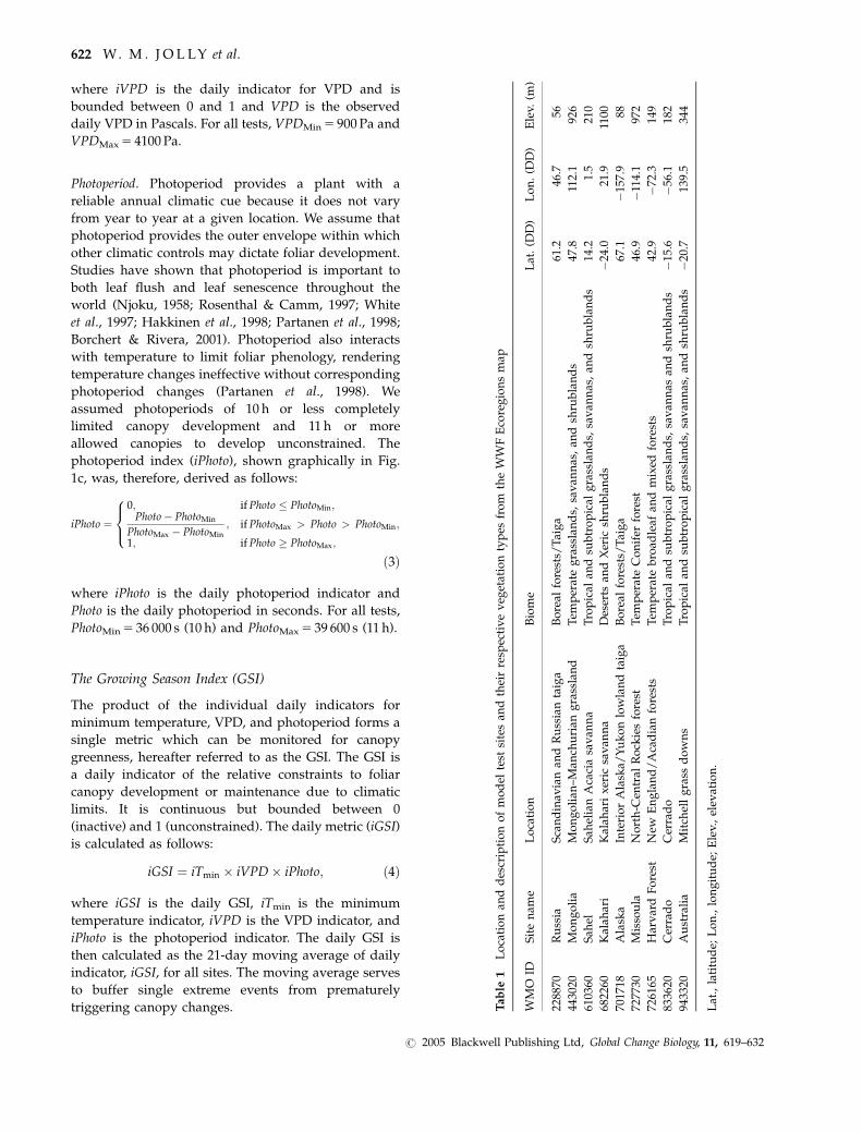
triggering canopy changes. Table

1Locationan

ddescriptionofmodel

test

sitesan

dtheirresp

ectiveveg

etationtypes

from

theW

WFEcoregionsmap

WMO

IDSitenam

eLocation

Biome

Lat.(D

D)

Lon.(D

D)

Elev.

(m)

228870

Russia

Scandinav

ianan

dRussiantaiga

Boreal

forests/

Taiga

61.2

46.7

56

4430

20Mongolia

Mongolian

–Man

churian

grassland

Tem

perategrasslands,

savan

nas,an

dsh

rublands

47.8

112.1

926

6103

60Sah

elSah

elianAcaciasavan

na

Tropical

andsu

btropical

grasslands,

savan

nas,an

dsh

rublands

14.2

1.5

210

6822

60Kalah

ari

Kalah

arixeric

savan

na

Deserts

andXeric

shrublands

�24

.021

.91100

701718

Alaska

InteriorAlaska/

Yukonlowlandtaiga

Boreal

forests/

Taiga

67.1

�15

7.9

88

7277

30Missoula

North-C

entral

Rockiesforest

Tem

perateConifer

forest

46.9

�114.1

972

7261

65HarvardForest

New

England/Acadianforests

Tem

peratebroad

leaf

andmixed

forests

42.9

�72

.314

9

8336

20Cerrado

Cerrado

Tropical

andsu

btropical

grasslands,

savan

nas

andsh

rublands

�15

.6�56

.118

2

9433

20Australia

Mitch

ellgrass

downs

Tropical

andsu

btropical

grasslands,

savan

nas,an

dsh

rublands

�20

.713

9.5

344

Lat.,latitude;

Lon.,longitude;

Elev.,elev

ation.



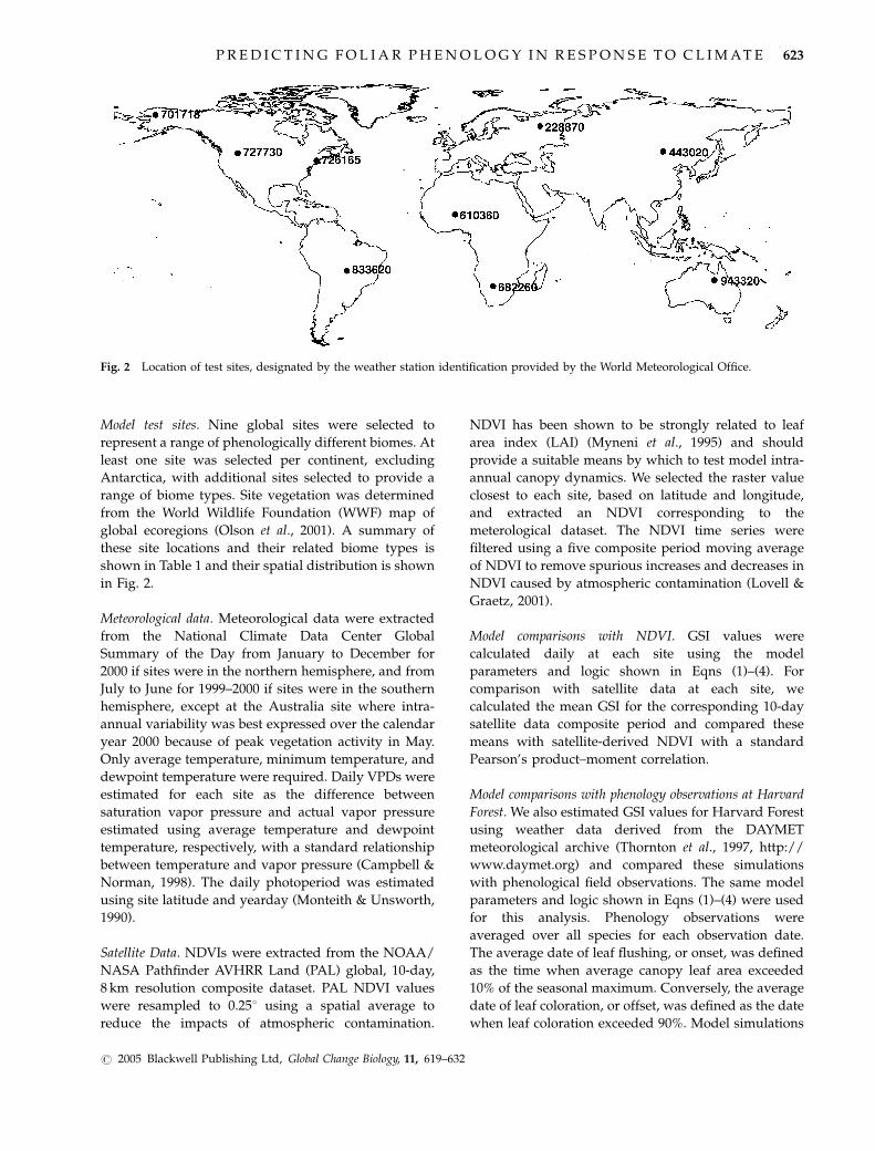
Model test sites. Nine global sites were selected to

represent a range of phenologically different biomes. At

least one site was selected per continent, excluding

Antarctica, with additional sites selected to provide a

range of biome types. Site vegetation was determined

from the World Wildlife Foundation (WWF) map of

global ecoregions (Olson et al., 2001). A summary of

these site locations and their related biome types is

shown in Table 1 and their spatial distribution is shown

in Fig. 2.

Meteorological data. Meteorological data were extracted

from the National Climate Data Center Global

Summary of the Day from January to December for

2000 if sites were in the northern hemisphere, and from

July to June for 1999–2000 if sites were in the southern

hemisphere, except at the Australia site where intra-

annual variability was best expressed over the calendar

year 2000 because of peak vegetation activity in May.

Only average temperature, minimum temperature, and

dewpoint temperature were required. Daily VPDs were

estimated for each site as the difference between

saturation vapor pressure and actual vapor pressure

estimated using average temperature and dewpoint

temperature, respectively, with a standard relationship

between temperature and vapor pressure (Campbell &

Norman, 1998). The daily photoperiod was estimated

using site latitude and yearday (Monteith & Unsworth,

1990).

Satellite Data. NDVIs were extracted from the NOAA/

NASA Pathfinder AVHRR Land (PAL) global, 10-day,

8 km resolution composite dataset. PAL NDVI values

were resampled to 0.251 using a spatial average to

reduce the impacts of atmospheric contamination.

NDVI has been shown to be strongly related to leaf

area index (LAI) (Myneni et al., 1995) and should

provide a suitable means by which to test model intra-

annual canopy dynamics. We selected the raster value

closest to each site, based on latitude and longitude,

and extracted an NDVI corresponding to the

meterological dataset. The NDVI time series were

filtered using a five composite period moving average

of NDVI to remove spurious increases and decreases in

NDVI caused by atmospheric contamination (Lovell &

Graetz, 2001).

Model comparisons with NDVI. GSI values were

calculated daily at each site using the model

parameters and logic shown in Eqns (1)–(4). For

comparison with satellite data at each site, we

calculated the mean GSI for the corresponding 10-day

satellite data composite period and compared these

means with satellite-derived NDVI with a standard

Pearson’s product–moment correlation.

Model comparisons with phenology observations at Harvard

Forest. We also estimated GSI values for Harvard Forest

using weather data derived from the DAYMET

meteorological archive (Thornton et al., 1997, http://

www.daymet.org) and compared these simulations

with phenological field observations. The same model

parameters and logic shown in Eqns (1)–(4) were used

for this analysis. Phenology observations were

averaged over all species for each observation date.

The average date of leaf flushing, or onset, was defined

as the time when average canopy leaf area exceeded

10% of the seasonal maximum. Conversely, the average

date of leaf coloration, or offset, was defined as the date

when leaf coloration exceeded 90%. Model simulations

Fig. 2 Location of test sites, designated by the weather station identification provided by the World Meteorological Office.



were performed daily from 1990 to 1997. Modeled leaf

onset was defined as the time when GSI exceeded 0.5 in

the spring and leaf offset was defined as the time when

GSI dropped below 0.5 in the fall. We computed the

mean absolute error (MAE) as the difference between

the predicted and observed yeardays of leaf onset and

leaf offset. Model predicted leaf onset dates were

compared with average observed leaf onset dates for

1990–1997. Model-predicted leaf offset dates were

compared with average observed leaf offset dates for

1991–1997. Our analysis was limited to this range of

dates because of differences in data availability for both

DAYMET and phenology observations.

Mapping global controls on vegetation foliar phenology

We used our generalized phenology model to calculate

the relative annual controls of VPD, minimum tem-

perature, and photoperiod spatially over the entire

globe. We utilized daily gridded climate data from the

National Center for Environment Prediction (NCEP)/

National Center for Atmospheric Research (NCAR)

Reanalysis (Kistler et al., 2001) for the year 2000 to

construct a global map of the factors that limit foliar

phenology. We calculated the point-wise daily indica-

tors for minimum temperature, VPD, and photoperiod

(Eqns (1)–(3), respectively) and summed each indicator

over the year. These indicators tell us the number of

days of the year that each variable was not limiting at a

given location. We then subtracted the annual point-

wise indicator sums from 365 to express each value in

terms of the number of days that it limits phenology in

a year. We calculated the actual vapor pressure from

surface air pressure and specific humidity and satura-

tion vapor pressure from average surface temperature.

VPD was calculated as the difference between satura-

tion and actual vapor pressures. Photoperiod was

estimated as a function of latitude and yearday

(Monteith & Unsworth, 1990). The temperature, VPD,

and photoperiod limits were then displayed as an Red/

Green/Blue (RGB) composite with each color repre-

senting a variable. VPD limits are displayed in red,

photoperiod limits are displayed in green and mini-

mum temperature limits are displayed in blue.

Results

The correlations between model-predicted GSI values

and satellite-derived NDVI values are shown in Table 2.

Using the same model and the same parameters we

were able to adequately predict the intra-annual

dynamics of the vegetation canopy at all sites regard-

less of the dominant or co-dominant climatic controls at

that site. There was a slight, but not marked, bias

towards better predictions at temperate sites. The

highest correlations were found in the high-latitude

forests, presumably because they are more purely

temperature limited than other sites. However, correla-

tions at the hydroperiodic sites were still very high,

suggesting that the VPD control adequately depicts the

intra-annual canopy dynamics in these regions.

Individual daily index values for minimum tempera-

ture, VPD, and daylength at each site are shown in Fig.

3. These figures clearly show the relative influence of

water, light, and temperature limitations at each site. In

only two cases does a single variable limit foliar

phenology (Fig. 3c, h). More often, there is a mix of

environmental limits both temporally, as shown when

observed over time at a given site, and spatially, as

shown when comparing sites.

Time-series plots of model-predicted foliar phenol-

ogy and NDVI values for each site are shown in Fig. 4.

In all cases, regardless of the previously reported

correlations, the GSI-predicted canopy dynamics ap-

pear to correspond well with observed canopy changes.

In some cases, the model predicted a drop in canopy

greenness after the initial start-of-season increase. For

example, at the Mongolia site, the start-of-season is

determined from temperature limits but the growing

season has high VPD. This is shown clearly in Fig. 3b

where the large red areas in midsummer indicate water

stress. During the period of the predicted canopy

activity drop, the rate of increase of NDVI is less than

the early season, suggesting that this VPD control may

be important in determining the rate of canopy

increase. In the Kalahari, early season conditions that

were not limiting were not met with concurrent

increases in canopy greenness. However, small con-

comitant increases and decreases between NDVI and

Table 2 Correlations between composite period NDVI va-

lues and modeled GSI values averaged over the composite

period for each of the nine test sites

WMO ID Location

Correlation between GSI

and NDVI

228870 Russia 0.939

443020 Mongolia 0.903

610360 Sahel 0.896

682260 Kalahari 0.742

701718 Alaska 0.986

726165 Harvard Forest 0.870

727730 Missoula 0.839

833620 Cerrado 0.868

943320 Australia 0.571

All correlations were significant (Po0.001).

NDVI, Normalized Difference Vegetation Index; GSI, Growing

Season Index; WMO, World Meteorological Office.



Fig. 3 The seasonal index values for minimum temperature, vapor pressure deficit, and daylength for each site showing the seasonal

limits of each variable. Indices are presented as a 21-day running average to better depict seasonal trends.



Russia

DateJan-00 May-00 Sep-00 Jan-01

GS

I

0.0

0.2

0.4

0.6

0.8

1.0

ND

VI

0.30

0.40

0.50

0.60

0.70Mongolia


GS

I

0.0

0.1

0.2

0.3

0.4

0.5

0.6

0.7

0.8

ND

VI

0.10

0.15

0.20

0.25

0.30

0.35

0.40

0.45

Sahel


GS

I

0.0

0.2

0.4

0.6

0.8

ND

VI

0.10

0.15

0.20

0.25

0.30Kalahari

DateJun-99 Oct-99 Feb-00 Jun-00

GS

I

0.0

0.2

0.4

0.6

0.8

1.0

ND

VI

0.10

0.15

0.20

0.25

0.30

0.35

0.40

0.45

Alaska


GS

I

0.0

0.2

0.4

0.6

0.8

1.0

ND

VI

0.10

0.20

0.30

0.40

0.50

0.60

0.70Harvard Forest


GS

I

0.0

0.2

0.4

0.6

0.8

1.0

ND

VI

0.50

0.55

0.60

0.65

0.70

0.75

Missoula


GS

I

0.0

0.2

0.4

0.6

0.8

1.0

ND

VI

0.30

0.40

0.50

0.60

0.70Cerrado

DateJun-99 Oct-99 Feb-00 Jun-00

GS

I

0.4

0.6

0.8

1.0

ND

VI

0.20

0.30

0.40

0.50

0.60

Australia


GS

I

0.2

0.4

0.6

0.8

1.0

ND

VI

0.220.240.260.280.300.320.340.360.380.400.42

Growing Season Index (GSI)NDVI

(i)

(g) (h)

(e) (f)

(c) (d)

(a) (b)

Fig. 4 A comparison of seasonal variation in the modeled Growing Season Index (GSI) with the Normalized Difference Vegetation

Index (NDVI) obtained from satellite coverage at 10-day intervals (see correlation coefficients in Table 2).



GSI values are observed during that period and the

model predicts a clear leaf flush as conditions become

more favorable. At Harvard Forest, the model over-

predicts increases in timing of observed increases in

canopy leaf area. However, modeled changes in canopy

greenness generally track well with observed changes

in canopy leaf area at all sites.

The results of model estimates of leaf onset compared

with observations is shown in Table 3 and leaf offset

comparisons are shown in Table 4. There was good

agreement between the modeled leaf onset and offset

dates and observations at Harvard Forest. The MAE of

predicted onset date compared with observed mean

onset date over 8 years was 3.38 days and the MAE of

predicted offset date over 7 years was 2.29 days. These

accuracies should not be overstated because a simple

mean yields an MAE of 4.25 and 2.14 days for onset and

offset, respectively. However, observed onset dates

were twice as variable as observed offset dates

(standard deviation of 6 days for onset compared with

3 days for offset), while prediction errors only differed

by about 1 day, suggesting that the model is robust to

interannual variability. This suggests that even though

the model predicts continuous changes in canopy

activity, it still serves well as a model to predict the

start and end dates of the foliage period.

The map of global climatic constraints to foliar

phenology is shown in Fig. 5. This map resolves major

global patterns of phenology while also revealing some

interesting patterns of interactive effects. Black areas in

the tropics show regions where climate is essentially

aseasonal; red areas show where water limits dominate

foliar phenology; blue shows where minimum tem-

peratures most limit phenology. Blue-green and green-

blue areas have co-limitations of photoperiod and

temperatures. The patterns depicted are consistent with

the global distribution of biomes that exhibit vastly

different leaf phenological strategies.

Discussion

In this paper, we have presented a new way of

assessing canopy foliar dynamics by combining

simple environmental limitations into an index that

quantifies changes in those limitations within the

year. We have succeeded in reproducing the intra-

annual canopy dynamics seen from satellite-derived

vegetation indices in various regions throughout the

world, independent of vegetation type, while using

the same type of input data, the same model and the

same model parameters. The model performs well in

multiple locations because it does not impose a priori

knowledge of vegetation or climate to switch dis-

cretely between models or model parameters; it

simply allows controlling climatic factors to shift or

co-limit both temporally and spatially.

A key component to this model, which promotes its

application to climate change scenarios, is this ability to

transition from one limiting factor to another without

the need for a discrete model change. As mentioned

earlier, previous attempts to model vegetation phenol-

ogy globally have required the discrete switching from

one model to another (Botta et al., 2000). Even in regions

that are small compared with the entire globe, different

factors limit foliar phenology spatially (Penuelas et al.,

2004). Therefore, a generalized phenology model must

provide sufficient flexibility to transition from one

limiting factor to another in both space and time.

In some cases, the model seemed to predict suitable

conditions when no observed changes in canopy were

evident. In the Kalahari, early season VPDs were low

and photoperiods were long, but no canopy changes

Table 3 Differences between model predicted and field

observed average leaf onset dates for Harvard Forests from

1990 to 1997

Observed average

onset date

Predicted

onset date

Absolute

difference

4/28/1990 5/1/1990 3

4/16/1991 4/24/1991 8

5/1/1992 5/6/1992 5

4/24/1993 4/25/1993 1

4/28/1994 4/30/1994 2

5/3/1995 5/3/1995 0

4/25/1996 5/2/1996 7

5/5/1997 5/6/1997 1

MAE (days) 3.38

The mean absolute error (MAE) of the model predictions was

3.38 days.

Table 4 Differences between model predicted and field

observed average leaf offset dates for Harvard Forests from

1991 to 1997

Observed average

offset date

Predicted

offset date

Absolute

difference

10/23/1991 10/25/1991 2

10/23/1992 10/20/1992 3

10/18/1993 10/19/1993 1

10/21/1994 10/20/1994 1

10/24/1995 10/28/1995 4

10/21/1996 10/22/1996 1

10/28/1997 10/24/1997 4

MAE (days) 2.29

The mean absolute error (MAE) of the model predictions was

2.29 days.



were observed. This may indicate inadequate model

variables or parameters in these locations, but it could

also suggest a difference in response time between

locations. Shallow-rooted plants may respond more

rapidly to environmental stimuli than deep-rooted

plants. In this case, model predictions of earlier canopy

initiation may not necessarily be wrong because we are

comparing the results with radiometrically averaged

NDVI values. If grasses account for only a small part of

the signal, they may be hidden in the overall time

series. We see a similar pattern at the Harvard Forest

site where model predictions increase earlier than

observed increases in NDVI. In similar locations,

understory plants flush leaves up to 2 weeks earlier

than overstory plants (Gill et al., 1998; Augspurger &

Bartlett, 2003), but the understory may contribute less

than 20% to the total LAI (Rhoads et al., 2002),

suggesting that the NDVI response may be more

dominated by larger vegetation.

Using VPD as a surrogate for precipitation has both

advantages and disadvantages. The main advantage is

that VPD is both continuous and easily calculated.

Global phenology studies have cited the low reliability

of precipitation and soil water potential data in the

tropics as the reason for poor predictions of foliar

phenology (Botta et al., 2000), due in part to the discrete

nature of precipitation. Precipitation, and its influence

on soil water storage, is a major driver of tropical

phenology. In many cases, leaf flush may be caused by a

single precipitation event (Childes, 1989). If the data for

that precipitation event were missing, this may intro-

duce a serious bias into a model. VPD is a continuous

variable and therefore would be less sensitive to a

single missing value.

The primary disadvantage of using VPD as a

surrogate for precipitation is that our model works on

the assumption that changes in VPD are a direct result

of seasonal precipitation changes. However, phenology

itself may influence VPD through transpiration. There-

fore, the main problem with using VPD in a prognostic

phenology model is whether or not changes in VPD are

a cause or effect: does VPD influence phenology or does

phenology influence VPD? We know that there is a

relationship between atmospheric water vapor pressure

and the date of leaf emergence at landscape scales

(Schwartz & Karl, 1990; Hayden, 1998) but the cause

and effect of this relationship is not clear. If either

advected moisture or precipitation raise vapor pres-

sures independent of vegetation feedbacks, then

changes in VPD could signal the onset of the rainy

season. However, if VPD decreases are primarily a

result of transpiration of newly flushed leaves, then this

method would not work as a prognostic model. It

would still work well as a monitoring model if using

observations rather than predicted VPDs. If integrated

into an ecosystem process model or a land-surface

model, soil water potential could be substituted for the

VPD control, using the same model framework. A

similar method has been shown to adequately predict

leaf area dynamics in some semiarid tropical regions

(Jolly & Running, 2004) and should correct any model

limitations caused by vegetation feedbacks.

Our model is independent of any particular applica-

tion and therefore could be incorporated into larger

modeling applications in a variety of ways. Although it

goes against our argument of creating a continuous

phenology model, we have shown that the model can

still be used as a discrete trigger telling other simulation

Fig. 5 Modeled regional constraints on phenology created from NCEP/NCAR weather data for the year 2000. In most regions, more

than one variable limits phenology. The black area in the tropics indicates no seasonal constraints.



models when to start growing leaves. Our model test at

Harvard Forest showed good agreement between

predicted and observed phenophase transition dates

even when using the same parameters and logic used

for all other sites. For this simple test, we defined a

threshold GSI value above which we assumed that

there is a plant canopy and below which you assume

there is no plant canopy. Our choice of 0.5 appears to be

a suitable threshold value. This cutoff value represents

the proportion of days in the smoothing window (21

days in this case) in which conditions were suitable for

a plant canopy. A value of 0.5 or greater simply means

that at least half of the days in the smoothing window

were sufficient to maintain a vegetative canopy.

Predicted leaf onset dates at Harvard Forest were

always greater than observations when we used 0.5 as

the GSI cutoff. This bias might suggest that this simple

cutoff may be too conservative. We encourage further

exploration of this cutoff value, and we also suggest

that this value may vary by species or biome. In theory,

this threshold could also be used with monthly

averages instead of daily running average values,

allowing it to be incorporated into ecosystem process

models that operate on monthly data such as the 3PG

model (Landsberg & Waring, 1997).

This model could also be used to generate dynamic

estimates of LAI by scaling the potential LAI for a site.

The model by definition is bounded between 0 and 1,

where 0 indicates times with a very low probability of a

plant canopy and 1 indicates a very high probability of

a canopy. Methods exist and have been tested in a

variety of regions for determining the optimal LAI for a

given site (Woodward, 1987; Nemani & Running, 1989).

Our simple phenology model could be used to scale

potential maximum LAI values for a site creating daily

estimates of LAI throughout the growing season.

The model parameters used in this analysis are

sufficient to reproduce large-scale differences in phenol-

ogy throughout the world but we do not contend that

these parameters are exactly the same everywhere. We

understand that different species and biomes are sensitive

to environmental conditions over different ranges of

values (Larcher, 1995). Rather, we have attempted to

provide a modeling framework and a simple set of

parameters that sufficiently resolve the heterogeneity of

phenology as observed from satellite data. Our efforts

were geared towards creating a generalized phenology

model, which is why we chose to develop a common set

of parameters and not vary them by site. However, one

should be able to tune the model to reproduce observed

variation in phenology at local scales.

In addition to the fixed environmental parameters,

we also chose a 21-day moving average because it

produced the most general results. By averaging over

21 days, model results are less erratic. We tested a

number of intervals from 7 to 21 days and found no

appreciable difference among the smoothing intervals

other than the desired effect of reducing erratic pulses

of model predictions from extreme climatic events that

were not indicative of average climatic conditions. It is

plausible that different life forms respond differentially

to changing environmental stimuli and that this

parameter may be biome-specific, but the model seems

to perform well for all biome types, suggesting our

choice of a 21-day averaging window is sufficient in

most locations. In fact, we improved correlations

between GSI model predictions and NDVI at the two

sites where the relationships were poorest were

improved if we increased the moving window from 3

to 6 weeks. Correlations between GSI and NDVI at the

Australia site improved from 0.57 to 0.75 and correla-

tions at the Kalahari improved slightly from 0.74 to 0.8.

These improvements were made without changing the

parameters of the individual index calculations. In-

creasing the moving window length likely represents

the longer term changes in soil water storage. The

model assumes that changes in soil water availability

are reflected as short-term changes in VPD; this moving

window size may ensure that this assumption is met.

However, throughout our discussion, we have empha-

sized the need for model generalization and that is why

we chose present model simulations at each site using a

21-day moving window. Furthermore, the choice of

smoothing window width also determines how fast the

model transitions from one phenological condition to

another, such as no leaves (0) to full canopies (1).

Similar values have been reported in other studies that

range from 21 to 31 days (Cleary & Waring, 1967; Van

Wijk et al., 2003).

Daily GSI values of one indicate that conditions were

optimal for plant growth during that day. It is

important to note that a GSI of one does not necessarily

correspond to an NDVI value of one because GSI is

independent of the vegetation cover and subsequent

correlations between absolute GSI and NDVI values

would be poor. However, if we sum daily GSI values

over a calendar year, we can obtain a more mechanistic

definition of growing season length and preliminary

comparisons between these annual GSI sums and

maximum annual NDVI indicate that they are strongly

related. Therefore, it may be possible to scale daily GSI

values to NDVI based on those annual totals.

Our map of phenological limiting factors is unique

because it displays regions where limiting factors are

either controlled by a single variable or an interaction of

variables. Phenology is co-limited by multiple factors in

many locations but these co-limitations have never

been expressed spatially for the globe. This map is



consistent with other studies that suggests co-limits in a

number of regions (Nilsen & Muller, 1981; White et al.,

1997; Jame et al., 1998; Nemani et al., 2003). The black

areas in the tropics define aseasonal climatic regions. In

these areas, photoperiod is the only likely abiotic cue

regulating canopy phenology. Indeed, in these areas,

vegetation responds to photoperiod changes of as little

as 15–30min (Njoku, 1958; Borchert & Rivera, 2001).

Pure temperature limits are rare and generally only

seen in alpine regions such as the Andes of South

America, the Rocky Mountains of North America, and

the Tibetan plateau of central Asia. Pure water-limited

phenology was more apparent over much of the globe.

The high latitudes, where solar radiation and tempera-

ture are highly seasonal, show a mix of photoperiod

and temperature limits which is consistent with

previous research (Partanen et al., 1998). Midlatitude,

temperate regions show more of a balance between

photoperiod controls and low temperature limits. We

hope that this map will better help researchers under-

stand the limits to global phenological patterns.

We have presented a simple, meteorological data-

based phenology model that can adequately predict the

intra-annual dynamics of plant canopies at sites through-

out the world using the samemodel logic and parameters

with no a priori knowledge of the local vegetation or

climate. We have demonstrated that this model is flexible

enough to predict phenology regardless of the factors

that control phenology regionally. We have used this

model to generate a global map of climate limits to foliar

phenology and we have found that it resolves spatial

patterns of areas with vastly different phenological

strategies. The model presented is simple and indepen-

dent of any particular modeling framework and thus

should be suitable for many global change applications.

Acknowledgements

We would like to thank Richard H. Waring, the editor and twoanonymous reviewers for constructive comments on earlierversions of this manuscript. This research was supported in partby funds provided by the Joint Fire Science Program and theRocky Mountain Research Station, Forest Service, US Depart-ment of Agriculture. We would like to thank John O’Keefe andthe Harvard Forest for diligently maintaining the scientificquality phenology dataset used in this study. We also wish tothank the Distributed Active Archive Center (Code 902.2) at theGoddard Space Flight Center, Greenbelt, MD, 20771, forproducing the data in their present form and distributing them.The original data products were produced under the NOAA/NASA Pathfinder program, by a processing team headed by Ms.Mary James of the Goddard Global Change Data Center; and thescience algorithms were established by the AVHRR Land ScienceWorking Group, chaired by Dr John Townshend of theUniversity of Maryland. Goddard’s contributions to theseactivities were sponsored by NASA’s Mission to Planet Earthprogram.

References

Augspurger CK, Bartlett EA (2003) Differences in leaf phenology

between juvenile and adult trees in a temperate deciduous

forest. Tree Physiology, 23, 517–525.

Bach CS (2002) Phenological patterns in monsoon rainforests in

the Northern Territory, Australia. Australian Journal of Ecology,

27, 477–489.

Borchert R, Rivera G (2001) Photoperiodic control of seasonal

development and dormancy in tropical stem–succulent trees.

Tree Physiology, 21, 213–221.

Botta A, Viovy N, Ciais P et al. (2000) A global prognostic scheme

of leaf onset using satellite data. Global Change Biology, 6, 709–

725.

Campbell GS, Norman JM (1998) Environmental Biophysics.

Springer-Verlag, New York, NY.

Chase TN, Pielke RA, Kittel T et al. (1996) Sensitivity of a general

circulation model to global changes in leaf area index. Journal

of Geophysical Research, 101, 7393–7408.

Childes SL (1989) Phenology of nine common woody species in

semi-arid, deciduous Kalahari Sand vegetation. Vegetatio, 79,

151–163.

Chuine I, Cour P (1999) Climatic determinants of budburst

seasonality in four temperate-zone tree species. New Phytol-

ogist, 143, 339–349.

Cleary BD, Waring RH (1967) Temperature: collection of data

and its analysis for the interpretation of plant growth and

distribution. Canadian Journal of Botany, 47, 167–173.

de Bie S, Ketner P, Paasse M et al. (1998) Woody plant phenology

in the West Africa savanna. Journal of Biogeography, 25, 883–900.

Foley JA, Levis S, Prentice IC et al. (1998) Coupling dynamic

models of climate and vegetation. Global Change Biology, 4,

561–579.

Gill DS, Amthor JS, Bormann FH (1998) Leaf phenology,

photosynthesis, and the persistence of saplings and shrubs

in a mature northern hardwood forest. Tree Physiology, 18, 281–

289.

Granier C, Tardieu F (1999) Water deficit and spatial pattern of

leaf development. Variability in responses can be simulated

using a simple model of leaf development. Plant Physiology,

119, 609–620.

Hakkinen R, Linkosalo T, Hari P (1998) Effects of dormancy and

environmental factors on bud burst in Betula pendula. Tree

Physiology, 18, 707–712.

Hayden BP (1998) Ecosystem feedbacks on climate at the

landscape scale. Philosophical Transactions of the Royal Society

of London, 353, 5–18.

Huffaker CB (1942) Vegetational correlations with vapor

pressure deficit and relative humidity. American Midland

Naturalist, 28, 486–500.

IPCC (2001) Climate Change 2001: The Scientific Basis. Contribution

of the Working Group 1 to the Third Assessment Report of the IPCC.

Cambridge University Press, Cambridge.

Jame YW, Cutforth HW, Ritchie JT (1998) Interaction of

temperature and daylength on leaf appearance rate in wheat

and barley. Agricultural and Forest Meteorology, 92,

241–249.

Jarvis P, Linder S (2000) Constraints to growth of boreal forests.

Nature, 405, 904–905.



Jolly WM, Running SW (2004) Effects of precipitation and soil

water potential on drought deciduous phenology in the

Kalahari. Global Change Biology, 10, 303–308.

Justice CO, Townsend JRG, Holben BN et al. (1985) Analysis

of the phenology of global vegetation using meteoro-

logical satellite data. International Journal of Remote Sensing, 4,

369–385.

Kang S, Running SW, Lim J-H et al. (2003) A regional phenology

model for detecting onset of greenness in temperate mixed

forests, Korea: an application of MODIS leaf area index.

Remote Sensing of Environment, 86, 232–242.

Keeling CD, Chin JFS, Whorf TP (1996) Increased activity of

northern vegetation inferred from atmospheric CO2 measure-

ments. Nature, 382, 146–149.

Kistler R, Kalnay E, Collins W et al. (2001) The NCEP–NCAR 50-

Year reanalysis: monthly means CD-ROM and documentation.

Bulletin of the American Meteorological Society, 82, 247–267.

Kramer K (1994) Selecting a model to predict the onset of growth

of Fagus sylvatica. Journal of Applied Ecology, 31, 172–181.

Landsberg JJ, Waring RH (1997) A generalized model of forest

productivity using simplified concepts of radiation-use

efficiency, carbon balance and partitioning. Forest Ecology and

Management, 95, 209–228.

Larcher W (1995) Physiological Plant Ecology. Springer-Verlag,

Heidelberg.

Larcher W, Bauer H (1981) Ecological significance of resistance

to low temperature. In: Encyclopedia of Plant Physiology, Vol.

12A (eds Lange OL, Nobel PS, Osmond CB, Ziegler H), pp.

403–437. Springer-Verlag, Berlin.

Lechowicz MJ (2001) Phenology. In: Encyclopedia of Global

Environmental Change (ed. Canadell J, Mooney HA), Vol. 2.

Wiley, London.

Levitt J (1980) Responses of Plants to Environmental Stresses.

Academic Press, New York.

Lieberman D (1982) Seasonality and phenology in a dry tropical

forest in Ghana. Journal of Ecology, 70, 791–806.

Lieth H (1974) Phenology and Seasonality Modeling. Springer,

Berlin, Germany.

Lovell JL, Graetz RD (2001) Filtering Pathfinder AVHRR Land

NDVI data for Australia. International Journal of Remote

Sensing, 22, 2649–2654.

Matsumoto K, Ohta T, Irasawa M et al. (2003) Climate change

and extension of the Ginkgo biloba L. growing season in Japan.

Global Change Biology, 9, 1634–1642.

Menzel A (2002) Phenology: its importance to the global change

community. Climatic Change, 54, 379–385.

Menzel A, Fabian P (1999) Growing season extended in Europe.

Nature, 397, 659.

Monteith JL, Unsworth MH (1990) Principles of Environmental

Physics. Edward Arnold, New York, NY.

Mott KA, Parkhurst DF (1991) Stomatal responses to humidity in

air and helox. Plant Cell and Environment, 14, 509–515.

Myneni RB, Keeling CD, Tucker CJ et al. (1997) Increased plant

growth in the northern latitudes from 1981 to 1991. Nature,

386, 698–702.

Myneni RB, Maggion S, Iaquinta J et al. (1995) Optical remote

sensing of vegetation: modelling, caveats and algorithms.

Remote Sensing of Environment, 51, 169–188.

Nemani RR, Keeling CD, Hashimoto H et al. (2003) Climate-

driven increases in global terrestrial net primary production

from 1982 to 1999. Science, 300, 1560–1563.

Nemani RR, Running SR (1989) Testing a theoretical climate–

soil–leaf area hydrologic equilibrium of forests using satellite

data and ecosystem simulation. Agricultural and Forest

Meteorology, 44, 245–260.

Nilsen ET, Muller WH (1981) Phenology of the drought–

deciduous shrub Lotus scoparius: climatic controls and adap-

tive significance. Ecological Monographs, 51, 323–341.

Njoku E (1958) The photoperiodic response of some Nigerian

plants. Journal of the West African Science Association, 4, 99–111.

Olson DM, Dinerstein E, Wikramanayake ED et al. (2001)

Terrestrial ecoregions of the World: a new map of life on

Earth. BioScience, 51, 933–938.

Osonubi O, Davies WJ (1980) The influence of plant water stress

on stomatal control of gas exchange at different levels of

atmospheric humidity. Oecologia, 46, 1–6.

Partanen J, Koski V, Hanninen H (1998) Effects of photoperiod

and temperature on the timing of bud burst in Norway spruce

(Picea abies). Tree Physiology, 18, 811–816.

Penuelas J, Filella I, Zhang X et al. (2004) Complex spatiotem-

poral phenological shifts as a response to rainfall changes.

New Phytologist, 161, 837–846.

Rhoads AG, Hamburg SP, Fahey TJ et al. (2002) Effects of an

intense ice storm on the structure of a northern hardwood

forest. Canadian Journal of Forest Research, 32, 1763–1775.

Rosenthal SI, Camm EL (1997) Photosynthetic decline and

pigment loss during autumn foliar senescence in western

larch (Larix occidentalis). Tree Physiology, 17, 767–775.

Salah H, Tardieu F (1996) Quantitative analysis of the combined

effects of temperature, evaporative demand and light on leaf

elongation rate in well-watered field and laboratory-grown

maize plants. Journal of Experimental Botany, 47, 1689–1698.

Schwartz MD (1999) Advancing to full bloom: planning

phenological research for the 21st century. International Journal

of Biometeorology, 42, 113–118.

Schwartz MD, Karl TR (1990) Spring phenology: nature’s experi-

ment to detect the effect of ‘green-up’ on surface maximum

temperatures. Monthly Weather Review, 118, 883–890.

Schwartz MD, Reiter BE (2000) Changes in North American

spring. International Journal of Climatology, 20, 929–932.

Sellers P, Los SO, Tucker CJ et al. (1996) A revised land surface

parameterization (SiB2) for atmospheric GCMs, II, The

generation of global fields of terrestrial biophysical para-

meters from satellite data. Journal of Climate, 9, 706–737.

Sparks TH, Carey PD (1995) The responses of species to climate

over two centuries, 1736–1947: an analysis of the Marsham

phenological record. Journal of Ecology, 83, 321–329.

Tenhunen JD, Hanano R, Abril M et al. (1982) The control by

atmospheric factors and water stress of midday stomatal

closure in Arbutus unedo growing in a natural macchia.

Oecologia, 55, 165–169.

Thornton PE, Running SW, White MA (1997) Generating

surfaces of daily meteorological variables over large regions

of complex terrain. Journal of Hydrology, 190, 241–251.

Van Wijk MT, Williams M, JA, GR (2003) Interannual

variability of plant phenology in tussock tundra: modelling



interactions of plant productivity, plant phenology, snowmelt

and soil thaw. Global Change Biology, 9, ;743–758.

Waring RH (1969) Forest plants of the eastern Siskiyous: their

environmental and vegetational distribution. Northwest

Science, 43, 1–17.

White MA, Thornton PE, Running SW (1997) A continental

phenology model for monitoring vegetation response to

interannual climatic variability. Global Biogeochemical Cycles,

11, 217–234.

White MA, Thornton PE, Running SW et al. (2000) Parameter-

ization and sensitivity analysis of the BIOME–BGC terrestrial

ecosystem model: net primary production controls. Earth

Interactions, 4, 1–85.

Woodward FI (1987) Climate and Plant Distribution. Cambridge

University Press, Cambridge.

Zimmerman MH (1964) Effect of low temperature on ascent of

sap in trees. Plant Physiology, 39, 568–572.



A generalized, bioclimatic index to predict foliar phenology in response to climate

Documents

Transcript of A generalized, bioclimatic index to predict foliar phenology in response to climate