UNF Digital Commons

UNF Graduate Theses and Dissertations Student Scholarship

1995

A General Theory of Geodesics with Applicationsto Hyperbolic GeometryDeborah F. LoganUniversity of North Florida

This Master's Thesis is brought to you for free and open access by theStudent Scholarship at UNF Digital Commons. It has been accepted forinclusion in UNF Graduate Theses and Dissertations by an authorizedadministrator of UNF Digital Commons. For more information, pleasecontact Digital Projects.© 1995 All Rights Reserved

Suggested CitationLogan, Deborah F., "A General Theory of Geodesics with Applications to Hyperbolic Geometry" (1995). UNF Graduate Theses andDissertations. 101.https://digitalcommons.unf.edu/etd/101

A GENERAL THEORY OF GEODESICS WITH APPLICATIONS TO HYPERBOLIC GEOMETRY

by

Deborah F. Logan

A thesis submitted to the Department of Mathematics and statistics

in partial fulfillment of the requirements for the degree of

Master of Science in Mathematical Sciences

UNIVERSITY OF NORTH FLORIDA

COLLEGE OF ARTS AND SCIENCES

July, 1995

The thesis of Deborah F. Logan is approved:

Chairperson

Accepted for the College of Arts and sciences:

Accepted for the University:

Dean of Graduate Studies

(Date)

~)q5 7/2()/C;.s-lL2AJi'Ji

j- 3/- '1..5 -

Signature Deleted

Signature Deleted

Signature Deleted

Signature Deleted

Signature Deleted

Signature Deleted

ACKNOWLEDGEMENTS

I wish to thank Dr. Leonard Lipkin for his guidance,

encouragement, and his thorough analysis of the contents of

this paper. This study of Differential Geometry has helped

me see the study of advanced mathematics as one big picture

rather than disconnected entities.

I appreciate the time and effort that Dr. Jingcheng

Tong and Dr. Faiz Al-Rubaee put into reading my thesis.

I wish to thank Dr. Champak Panchal and Dr. Donna Mohr

for their planning of my graduate program and their

guidance throughout.

Last, but not least, I want to extend my gratitude

and love to my husband, Charlie, and my three children,

Jonathan, April, and Philip. They have supported and

encouraged me dur~ng my graduate studies.

iii

TABLE OF CONTENTS

Page

ABSTRACT ... v

INTRODUCTION • . 1

Chapter I. MANIFOLDS AND GEODESIC THEORY

1. Manifolds . . . . . . . 3

2. Riemannian Manifolds. . 15

3. Geodesics . . 24

4. Curvature .. 37

5. Cut Locus . 45

6. Geodesic Circles, Normal Neighborhoods, and Conjugate Points. . .. 49

7. Gauss-Bonnet Theorem. . 61

Chapter II. NON-EUCLIDEAN GEOMETRY

1. Beltrami Disk . 64

2. Poincare Disk 71

3. Poincare Half-Plane

A. Geodesics and Curvature 81

B. Relationship Between Euclidean Circles and Hyperbolic Circles. 88

C. Rigid Motions . . . . . . . .. 89

D. Geodesic Triangles 99

BIBLIOGRAPHY . . . 108

VITA . • • • . • 110

iv

ABSTRACT

A General Theory of Geodesics

With Applications to Hyperbolic Geometry

In this thesis, the geometry of curved surfaces is

studied using the methods of differential geometry. The

introduction of manifolds assists in the study of classical

two-dimensional surfaces. To study the geometry of a

surface a metric, or way to measure, is needed. By

changing the metric on a surface, a new geometric surface

can be obtained. On any surface, curves called geodesics

play the role of "straight lines" in Euclidean space. These

curves minimize distance locally but not necessarily

globally. The curvature of a surface at each point p

affects the behavior of geodesics and the construction of

geometric objects such as circles and triangles. These

fundamental ideas of manifolds, geodesics, and curvature

are developed and applied to classical surfaces in

Euclidean space as well as models of non-Euclidean

geometry, specifically, two-dimensional hyperbolic space.

v

INTRODUCTION

The geometry of curved surfaces has been studied

throughout the history of mathematics. The development

of the calculus enabled the theory of curves to flourish.

It enabled a deeper study of curved surfaces that led to a

better understanding and generalization of the whole

subject. It was discovered that some properties of curved

surfaces are intrinsic properties, that is, they are

geometric properties that belong to the surface itself and

not the surrounding space.

To study the geometry of a surface, we need a metric,

or a way to measure. Any property of a surface or formula

that can be deduced from the metric alone is intrinsic. By

changing the metric on a surface, we will obtain a new

geometric surface. The two-dimensional plane with the

Euclidean metric gives rise to the Euclidean plane. The

two-dimensional.plane with the Poincare metric gives rise

to a model of non-Euclidean geometry called the Poincare

half-plane. This geometric surface will be studied in

section three of chapter two.

The methods of differential geometry are used to study

the geometry of curved surfaces. Differential geometry

deals with objects such as tangent vectors, tangent fields,

tangent spaces, differentiable functions on surfaces, and

curves. The introduction of manifolds (a generalization of

surfaces) will assist in the study of classical two-

dimensional surfaces.

On any manifold, there are special curves called

geodesics. These are curves that play the role of

"straight lines" in Euclidean space. These curves minimize

distance locally but do not necessarily minimize distance

globally. From this fact comes the concept of convex

neighborhoods, that is, neighborhoods in which pairs of

points can be joined to each other by a unique minimizing

geodesic.

An important property of a manifold is how the manifold

is curving at each point P. Curvature affects the behavior

of geodesics, the measure of angles, as well as the sum of

the interior angles of geodesic triangles constructed on

the manifold.

In chapter one, the fundamental ideas of manifolds,

geodesics, and curvature are developed. In this chapter,

these fundamental- ideas are applied to classical surfaces

in Euclidean space. In chapter two, a thorough study is

done of models of non-Euclidean geometry, specifically,

two-dimensional hyperbolic space. This study includes

geodesics and curvature as well as geodesic triangles,

hyperbolic circles, congruences, and similarities.

2

1. Manifolds

CHAPTER 1

MANIFOLDS AND GEODESIC THEORY

1.] Definjtion. A geometric surface is an abstract surface

M furnished with an inner product,· on each of its

tangent planes. This inner product is required to be

differentiable in the sense that if V and Ware

differentiable vector fields on M, then V ·w is a

differentiable real-valued function on M.

Each tangent plane of M at the point P has its own inner

product. This inner product is a function which is

bilinear, symmetric, and positive definite. An assign-

ment of inner products to tangent planes is called a

geometric structure or metric tensor on M. Therefore,

the same surface -furnished with two different geometric

structures gives rise to two different geometric surfaces.

The two-dimensional plane, with the usual dot product

on tangent vectors <v,w>= V1Wl + V 2W2 ' is the best-known

geometric surface. Its geometry is two-dimensional

Euclidean geometry. A simple way to get new geometric

structures is to distort old ones. Let g > 0 be any

differentiable function on the plane.

3

Define

v ·W =

for tangent vectors v and w to the two-dimensional plane

at P. This is a new geometric structure on the plane. As

long as g2(p) + 1, then the resulting geometric surface has

properties quite different from the Euclidean plane.

In studying the geometry of a surface, some of the most

important geometric properties belong to the surface itself

and not the surrounding space. These are called intrinsic

properties. In the nineteenth century, Riemann concluded

the following: There must exist a geometrical theory of

surfaces completely independent of R3. The properties of a

surface M could be discovered by the inhabitants of M

unaware of the space outside their surface.

At first, Riemannian geometry was a development of the

differential geometry of two-dimensional surfaces in R3.

From this perspec"tive, given a surface S c R3, the inner

product <v,w> of two vectors tangent to S at a point P of

S is the inner product of these vectors in R3. This yields

the measure of the lengths of vectors tangent to S. To

compute the length of a curve, integrate the length of its

velocity vector.

~ Defjoitloo. A regular curve in RJ is a function

a: (a,b)-RJ which is of class Ck for some k~l and for

4

which da/dt+ 0 for all t E (a,b). A regular curve

segment is a function a:[a,b]-R3 together with an

open interval (c,d), with c<a<b<d, and a regular curve

y:(c,d)-R3 such that a(t)=y(t) for all tE [a,b].

~ Definition. The length of a regular curve segment

a: [a,b]--+R 3 is Jab Ida/dtl dt.

The definition of inner product allows us to measure

area of domains in S, the angle between two curves, and all

other "metric" ideas in geometry. certain special curves on

S, called geodesics, will be a major focus in this thesis.

These curves play the role of straight lines in Euclidean

geometry.

The definition of the inner product at each point PES

yields a quadratic form I p, called the first fundamental

~ of S at P, defined in the tangent plane TpS by

Ip(v) = <v,v>, V E TpS. In 1827, Gauss defined a notion of

curvature for surfaces. Curvature measures the amount that

S deviates, at a point PES, from its tangent plane at P.

Curvature, as Gauss defined it, depended only on the manner

of measuring in.S, which was the first fundamental form of

S at P. Curvature will be discussed in section four of this

chapter.

During Gauss' time, work was done to show that the

fifth postulate of Euclid was independent of the other

postulates of geometry. Euclid's fifth (parallel postulate)

says [13]: "Given a straight line and a point not on the

5

line then there is a straight line through the point which

does not meet the given line." It was also earlier shown

that this postulate is equivalent to the fact that the sum

of the interior angles of a triangle equals 180°. This led

to a new geometry that depended on a fundamental quadratic

form that was independent of the surrounding space. In this

geometry, straight lines are defined as geodesics and the

sum of the interior angles of a triangle depends on the

curvature.

In 1854, Riemann continued working on Gauss' ideas

and introduced what we call today a differentiable manifold

of arbitrary dimension n. Riemann associated to each point

of the manifold a fundamental quadratic form and generalized

the idea of curvature. Riemann was interested in the

relationship between physics and geometry. This

relationship motivated the development of non-Euclidean

geometries.

~ Defjnjtjon. f:R~R is of class ~k if all derivatives

up through order k exist and are continuous. f:RA~R

is of class ~k if all its (mixed) partial derivatives

of order k and less exist and are continuous. A

function f:RA~RP is of class ~k if all its components

with respect to a given basis are of class ek•

The concept of a differentiable manifold is necessary for

extending the methods of differential calculus to spaces

6

more general than Rn. An example of a manifold is a

regular surface in R3.

~ pefjnition. A Ck coordinate patch (regular surface) is

a one-to-one Ck function x:U-R 3 for some k ~ 1, where

U is an open subset of R2 with coordinates u l and u2 and

(ax/au 1) X (ax/au2

) + (5 on U.

The mapping x is called a parametrization of S at p.

A regular surface is intuitively a union of open sets of

R2, organized in such a way that when two such open sets

overlap, the change from one to the other can be made in

a differentiable manner. The problem with this definition

is its dependence on R3. The definition of a

differentiable manifold will be given for an arbitrary

dimension n. Differentiable will always mean a class of C·.

~ pefinition. A differentiable manifold Q! dimension n

is a set M and a family of one-to-one mappings

x..:Ua c Rn - M of open sets Ua of Rn into M such that:

(1) U a xa (Ua) = M.

(2) for any. pair ex,B with Xa(Ua ) n XB(UB) = W + 0, the

sets XB -1 (W) and Xa -1 (W) are open sets in Rn and the

mappings XB -1 0 Xa are differentiable.

(3) The family {(Ua,Xa)} is maximal relative to the

conditions (1) and (2), i.e., the family {(Ua,Xa)}

contains all possible mappings with these

properties.

The pair (Ua , Xa) with P E Xa (Ua ) is called a parame-

7

trization or system of coordinates of M at P. Xa(Ua) is

then called a coordinate neighborhood at P. A family

{(Ua,Xa)} satisfying (1) and (2) is called a differentiable

structure on M.

FIGURE ~

A differentiable structure on a set M induces a natural

topology on M. Define A c M to be an open set in

M if and only if Xa-1 (A n Xa (Ua» is an open set in

Rn for all a. The topology is defined such that

the sets Xa(Ua) are open and that the mappings Xa are

continuous. The Euclidean space Rn is an n-manifold with

the family of mappings generated by (R n, identity).

Similarly, any open set in Rn is an n-manifold.

~ Example. Let G=GL(n,R) be the group of all non-

singular nxn matrices. We show that G is an n 2-dimensional

manifold. G is a metric space with distance function

d(A,B)=.jt(ajj -bjj )2 where A=(aij) and B=(bij ). If A=(aij)EG,

let

8

Define a function V': RA2~R by

V' (xu, .•• , xnn ) =Lo£sn (-1) ° XI,o(l) X2,o(2) ... xn,o(n) ,

where Sn is the group of permutations on n letters.

It can be shown that V' is continuous and V'o~(A)=detA.

Therefore ~(G)= VI(R-{O}) is open. Let M(n) be the set of

all nxn matrices. We have identified M(n) and RA2 by the

mapping ~.

For surfaces in R3, a tangent vector at a point P of

the surface is defined as the "velocity" in R3 of a curve

in the surface passing through P. For differentiable

manifolds, we do not have the support of the surrounding

space. In elementary calculus, a vector v at a point

P E Rn may be viewed as a directional derivative. If

v = (a1 ,a2 , ••• ,an) and f:R n -R is differentiable, then the

non-normalized directional derivative of f at P in the

direction v is

v (f) = ~ a i (afjaui) (P) .

This concept will be used to define a tangent vector as a

real-valued operator on the set of differentiable

functions on M which obeys the properties of a derivative.

Let D(M) "denote the set of all local smooth (C·)

functions at the point x in the smooth (C-) manifold M. By

a local smooth function at the point x of M, we mean a

smooth (C-) function f:U-R defined on an open neighborhood

U of x in M. In the set D(M) define scalar multiplication,

addition, and multiplication as follows.

9

For arbitrary a,b E R and any two local smooth

functions f:U-R, g:V-R in O(M) , we have the local

smooth functions

defined by

af + bg: U n V -R

fg: U n V -R

( a f + bg) (w) = a [ f (w)] + b [ 9 (w) ] ,

(fg) (w) = f (w) 9 (w)

for every w E U n V. These operations fail to make O(M)

an algebra over R. O(M) is not a linear space over R

because f + (-f) + 9 + (-g) unless U = V. To correct

this problem, define a relation - in the set O(M) as

follows. For any two local smooth functions f:U-R

and g:V-R in O(M), f - 9 if and only if there exists

an open neighborhood W c U n V of x in M such that

f(w) = g(w) holds for every point w in w. since this

relation in O(M) is reflexive, symmetric, and transitive,

it is an equivalence relation. Therefore - divides the

members of O(M) into disjoint equivalence classes called

the germs of local smooth functions at the point x of M.

Let G(M)=O(M)j- denote the set of all smooth germs

at the point x of M and let p:O(M) - G(M) denote the

natural projection of the set O(M) onto its quotient set

G(M). Oefine scalar multiplication, addition, and

multiplication in G(M) for arbitrary smooth germs w,8 E

G(M), a,b E R, fEW, and gEe as follows:

10

aw + be = p(af + bg)

we = p(fg)

These operations make G(M) the algebra of smooth germs

at the point x in M of C· functions.

~ pefinition. A tangent vector to M at P is a function

Xp:D(M)-R whose value at f is denoted by Xp (f), such

that for all f,g E D(M) and r E R,

(a) Xp(f + g) = Xp(f) + Xp(g);

(b) Xp(rf) rXp(f); and

(c) Xp(fg) = f(P)Xp(g) + g(P)Xp(f),

where fg is the ordinary product of functions f and g

and f(P)Xp(g) is the product of real numbers f(P) and

Xp(g). Xp(f) may be read as the non-normalized

directional derivative of f in the direction Xp at P.

Let a:(-e,e)-M be a differentiable curve in M with

a(O) = P. Let X: be defined by X:(f) = (d(foa)jdt) (0) .

Let D be the set of functions on M that are differentiable

at P. The tangent vector to the curve a at t=o is a

function Xpa :D-R .given by

Xpa(f) = d(foa)jdtlt~O' fED.

The tangent vector at P is the tangent vector at t=o to

the curve a:(-e,e)-M with a(O) = P. The set of all

tangent vectors to M at P will be indicated by TpM.

Let x:U-Mn at P=x(O) be a parametrization where

n indicates the dimension of M. Express the function

f:Mn-R and the curve a in this parametrization by

11

fox(q)=f(xl ..... xn)' q= (Xl, ••• ,Xn) E U,

and x-loa (t) = (Xl (t) , .•• , Xn (t) ) .

Restricting f to a we obtain

Xpo (f) = (d/dt) (foa) I teO = (d/dt) f (xdt) , .•• , Xn (t) ) I teO

= ~ (dxddt) I t=O (Bf/Bxd = p: Xi' (0) (B/Bxd 0) f.

FIGURE 2.

Therefore, the vector Xpo can be expressed in the parame-

trization x by

Xpo = ~ Xi' (0) (B/Bxdo.

(B/Bxd 0 is the tangent vector at P of the "coordinate

curve": Xi-X(O'.~ .. 'O'Xi'O' .•. ,O). Therefore the tangent

vector to the curve a at P depends only on the derivative

of a in a coordinate system.

~ Defjnition. The tangent space ~ M ~ £, TpM, is the

set of all tangent vectors to M at P. The set

TpM, with the usual operations of functions,

forms a vector space of dimension n.

The choice of a parametrization x:U-M determines an

12

associated basis {(ajaX1)O, ••• , (ajaxn)o} in TpM. The linear

structure in Tpm defined above does not depend on the

parametrization x.

~ Defjnition. Let M and N be differentiable manifolds.

If ~:M-N is differentiable, the differential of ~ at

P is the function

(~ .. )p:TpM - Tcp(p)N

defined by

(~ .. )p(Xp) (f)

where Xp E TpM, fED (N) .

~ proposition. Let~: M - Nand P E M. Then

(~ .. ) p: TpM - T~(p)N is a linear transformation.

Proof: Let r E R, Xp, Yp E TpM. We need to show that

(~ .. )p(rxp + Yp) = r(~ .. )pXp + (~")pYp. For any f E D(N):

«~ .. ) p(rXp + Yp» (f) = (rXp + Yp) (fo~)

= rXp(fo~) + Yp(fo~) = r(~")p(Xp)f + (~")p(Yp)f

= (r(~ .. )pXp + (~")pYp) (f) QED

~ Defjnition. Let Mn and Nffi be differentiable manifolds

of dimension~ nand m, respectively. M is an

embedded sllbmapjfold of N is there is a differenti-

able function ~:M - N such that ~ is one-to-one and

(~.)p is one-to-one for each P E M.

If M is a submanifold of N, then dim M ~ dim N. The

tangent space to M can be viewed as a subspace of the

tangent space to N.

1.13. Defjpjtiop. A vector field X on a differentiable

13

manifold M is a correspondence that associates to each

point P E M a vector Xp E TpM.

~ Definitjon. A vector field X on a differentiable

manifold M is differentjabJe in the following sense:

if f is a differentiable function on M, then the

mapping P-Xpf is differentiable.

Let X(M) represent the set of all vector fields on M. If

X,Y E X(M), r E R, and f E D(M), then:

(X + Yh = Xp + Yp , (rX)p = r"Xp, and

( fX h = f (P) Xp •

~ pefjnition. If X, Y E X(M), then the Lie Bracket of

X and Y, [X,Y], is the vector field defined by

[X,Y]pf = Xp(Yf) - Yp(Xf) for f E D(M) and P E M.

~ Lemma. [X,Y] is vector field on M.

(See Millman and Parker,[9])

~ Propositjon. If X,Y,Z E X(M) and r E R, then

(a) [X,Y] = -[Y,X] and [rX,Y] = r[X,Y]

(anticommutativity)

[X,Y] = XY -. YX = -[YX - XY] = -[Y,X]

[rX,Y] = rXY - YrX = r[XY-YX] = r[X,Y].

(b) [X + Y,Z]' ~ [X,Z] + [Y,Z] and [Z,X + Y]

[Z,X] + [Z,Y] (linearity).

(c) [[X,Y],Z] + [[Y,Z],X] + [[Z,X],Y] = 0

(Jacobi's Identity)

14

2. Riemannian Manifolds

Riemannian geometry is a generalization of metric

differential geometry of surfaces. Instead of surfaces, one

considers n-dimensional Riemannian manifolds. These are

obtained from differentiable manifolds by introducing a

Riemannian metric. The corresponding geometry is called

Riemannian geometry. Surfaces are two-dimensional

Riemannian manifolds. These concepts will be discussed in

this section.

2.1 Defjnjtjon. A Riemannjan metric (or Riemannian

structure) on a differentiable manifold M is a

correspondence which associates to each point P of M

an inner product <,>p (that is, a symmetric, bilinear,

positive definite function) on the tangent space TpM

which varies differentiably in the following sense.

If x:UcR n - M is a system of coordinates around

P, with X(X1 ,X2 , ••• xll)= q E X(U), then

a a <-,-> = gij(X1,···,x) ax.1 aX:J q 11

is a differentiable function on U.

This definition does not depend on the choice of coordinate

system. The function gij(Xl, ... ,Xn ) is called the local

representation of the Riemannian metric in the coordinate

system x:UcRn - M. A differentiable manifold with a given

Riemannian metric is called a Riemannian manifold.

When are two Riemannian manifolds M and N the same?

2.2 Definitjon. Let M and N be Riemannian manifolds.

15

A diffeomorphism f:M - N (that is, f is a

differentiable bijection with a differentiable inverse)

is called an isometry if:

(*) <il,V>p=«f.)p(il) , (f.)p(v»r{p) '

for all P E M, il,v E TpM.

2.3 Defjnition. Let M and N be Riemannian manifolds. A

differentiable mapping f:M - N is a local isometry at

P E M if there is a neighborhood U c M of P such that

f:U - f(U) is a diffeomorphism satisfying (*).

Commonly, it is said that a Riemannian manifold M is

locally isometric to a Riemannian manifold N if for

every P in M there exists a neighborhood U of P in M

and a local isometry f:U - f(U) c N.

Some examples of the notion of Riemannian manifold are

as follows.

2.4 Example. Let M = an with a/axi identified with

ei=(O, ••• ,1, ... ,0). The metric is given by <eil ej> = Oij.

an is called Euclidean space of dimension n and the

Riemannian geometry of this space is metric Euclidean

geometry.

2.5 Example. "The product metric. Let Ml and Mz be

Riemannian manifolds and consider the cartesian product

Ml X Mz with the product structure.

Let ~:~~ .. ~ and ~:~~ .. ~ be the natural

projections. (See Do Carmo, [3]) Introduce on Ml X Mz a

Riemannian metric as follows:

16

<il, V> (pq) =< (~) ;il, (~) ;V>p + < (~) ;il, (~) ;V> q ,

for all (p, q) E Ml X M2, il, vET (pq) (Ml X Mz) •

The torus S1X ••• XS1 = Tn has a Riemannian structure obtained

by choosing the induced Riemannian metric from R2 on the

circle S1 c R2 and then taking the product metric. The

torus Tn with this metric is called the flat torus.

A differentiable mapping a:I-M of an open interval

I c R into a differentiable manifold M is called a

(parametrized) curve. A parametrized curve can self-

intersect as well as have "corners".

I

FIGURE 3

2.6 Definitj on. 'A vector field V along a curve a: I-M is

a differentiable mapping that associates to every t E I

a tangent vector vet) E Ta(t)M. The vector field

a+(d/dt), denoted by da/dt, is called the velocity

field (or tangent vector field) of a.

I is a one-dimensional manifold with tangent vector d/dt

as a basis. The restriction of a curve a to a closed

interval [a,b] c I is called a segment. If M is a

17

Riemannian manifold, the length of a segment is defined

by

1 b = Ib < da, da >112 dt. • • dt dt

Let X(M) be the set of all vector fields of class c· on M and let G(M) be the algebra of germs of C· (smooth)

functions. In order to study the change in a vector field

with respect to a direction, we introduce the notion of

differentiation of vector fields.

2.7 Definjtion. A linear connection ~ on a differentiable

manifold M is a mapping ~: X(M) X X(M) - X(M) which

is denoted by <X, Y> 'V_ ~xY and which satisfies the

following properties:

3) ~xfY = (Xf)Y + f~xY; X,Y,Z E X(M) and f,g E O(M).

~xY should be read as the covariant derivative of Y in the

direction of X.

Since many developments in the geometry of manifolds

are local, we specify a connection by its local coordinates

as follows.

2.8 pefinitjon.· Let ~ be a connection on M and let

X:OCRA~M be a system of coordinates about P. The

Chrjstoffel symbols of ~ with respect to the system of

coordinates are the functions r i / E O(x(U» defined by

VZI

Xj = Va/&x1

(O/OXj ) = Lk r i / (a/axk) = Lk r i / Xk •

This shows that there are infinitely many connections on

18

a manifold which can be obtained by prescribing the

Christoffel symbols (subject to symmetry conditions).

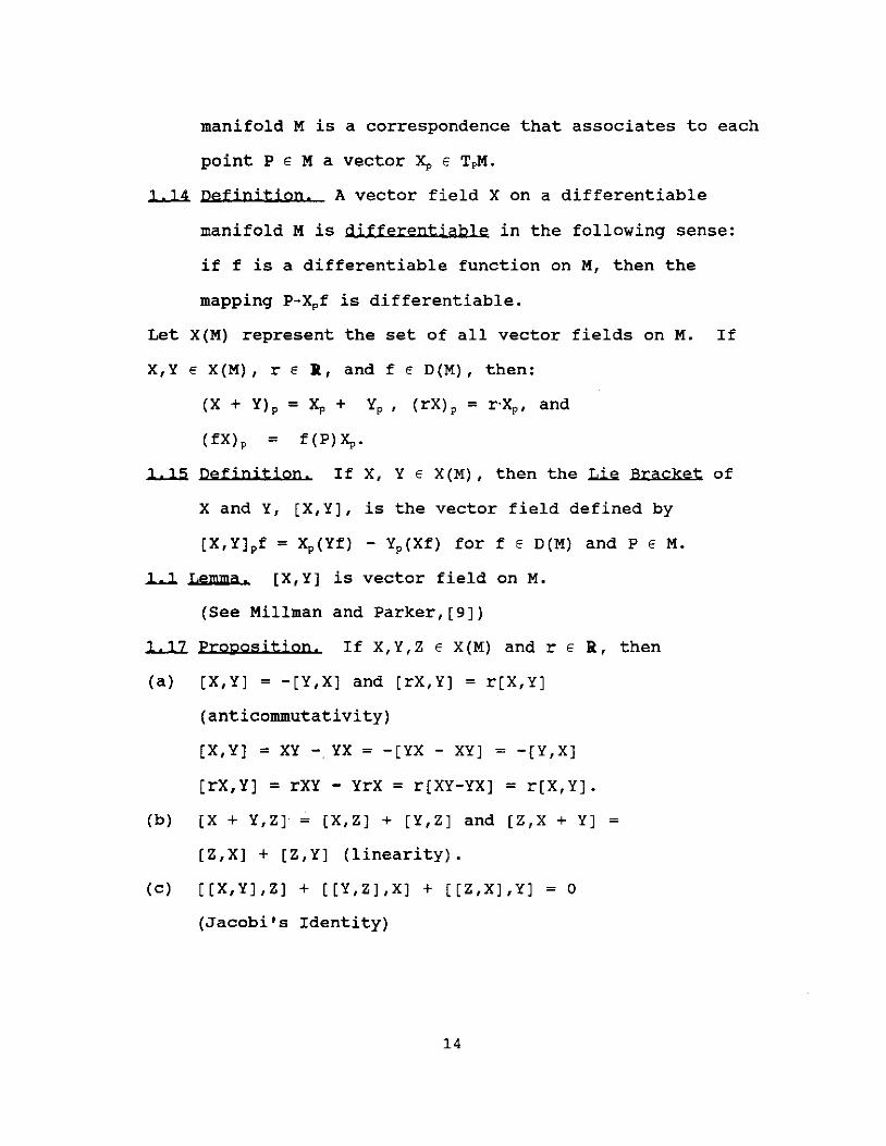
2.9 Example. (Flat Euclidean space).

Let M=Rn. If Y E X(lln) , then Y = Lfiei for some fi E D(Rn).

Define the flat conncection on Rn by VxY = LdXfi) ei.

By definition, this defines a linear connection on the

manifold :an.

VX1Xj= a for all i and j so that r i/ = a for all i,j,k.

VxY is the usual directional derivative of a vector-valued

function.

2.10 Example. Let M be flat Euclidean 2-space,

ex(t) = (cos t, sin t) for a < t < 2n and Y = yel - xe2.

Since T = -sintel + coste2, let X = -yel + xe2 so that

Xa(t) = Ta(t). If follows that 'ilTY = 'ilxY = Xyel - Xxe2

= xel + ye2 and 'ilTY = costel + sinte2.

Other connections will be discussed in section three of

this chapter.

In the Euclidean plane, two lines are parallel if

they have the same slope. Two curves ex,B:I-R 3 are parallel

if their tangent vectors exl(s) and BI(S) are parallel for

each s in I, which implies that their tangent vectors have

the same slope for each s in I.

2.11 Definition. Let M be a differentiable manifold with

a linear connection 'il. Let ex:I-M be a differentiable

curve in M. A vector field V along a curve ex:I-M is

called paraJJel when 'ilTV = DV/dt = 0, for all t E I.

19

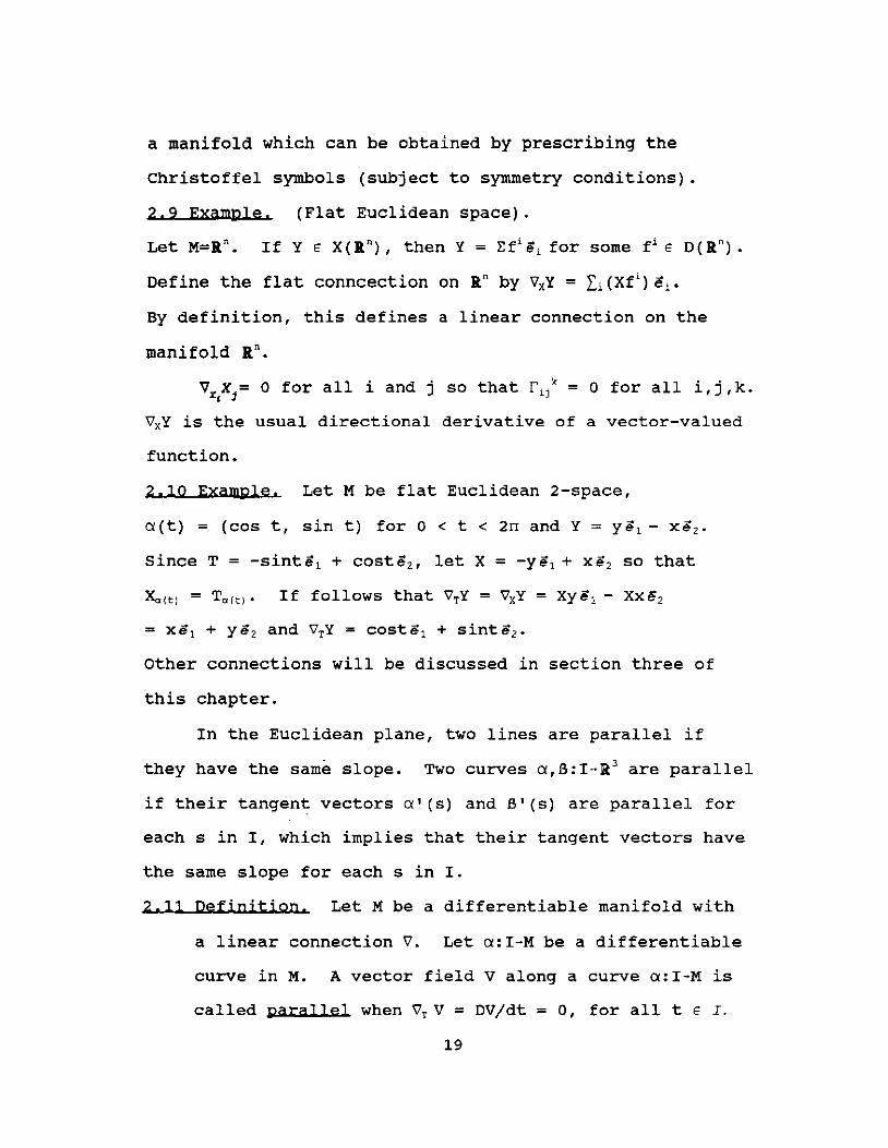
2.12 Proposition. Let M be a differentiable manifold

with a linear connection V. Let a:I-M be a differentiable

curve in M and let Vo be a vector tangent to M at aCto),

to E I. Then there exists a unique parallel vector

field vet) along a, such that Veto) = vo' vet) is called

the parallel transport of veto) along a.

(See Do Carmo, [3])

As a consequence of this proposition, if there exists a

vector field V in X(U) which is parallel along a with

veto) = Vo, then

o = ~~ = Lj (dvjjdt)Xj + L,j(dxjdt)vj VX1

Xj

where V = Lj v j Xj and Vo = Lj voj Xj . setting 'VX1

X j =Lk fi/ Xk

and replacing j with k in the first sum, we obtain DV dt

k . k = Lk {(dv jdt) + Lij v J (dxjdt) r ij }Xk = o. The system of n differential equations in Vk(t) ,

k k . o = dv jdt + L,j r ij v J (dxjdt), k=l, ... ,n,

possesses a unique solution satisfying the initial

2.13 Definition. A linear connection V on a smooth

manifold Mis said to be symmetric when

[X,Y] for all X,Y E X(M).

Local Riemannian geometry is concerned only with the

differential geometric properties of a part of a

differentiable manifold which can be covered by one

system of coordinates. The fundamental theorem of local

20

Riemannian geometry states that with a given Riemannian

metric there is uniquely associated a symmetric linear

connection with the property that parallel transport

preserves inner products. This unique linear connection

is called the Riemannian connection of the Riemannian

manifold.

2.14 Definition. Let V be a vector field along a curve a,

and let T be its tangent vector. V is parallel along a

if V'T V = DV / dt = o.

2.15 Definition. Let M be a differentiable manifold with a

linear connection V' and a Riemannian metric <,>. A

connection is said to be cornpatjble with the metric

<,>, when for any smooth curve a and any pair of

parallel vector fields V and V' along a, then <V, V'> =

constant.

2.16 proposjtion. Let M be a Riemannian manifold. A

connection V' on M is compatible with a metric <,> if and

only if for any vector fields V and W along the differenti-

able curve a:I-M we have d -<V,w> = dt

<V'TV, W> + <V'V'TW> = < DV W> + <V DW> , tEl. dt ' , dt

This implies that if V' is compatible with a Riemannian

metric <,>, then we are able to differentiate the inner

product using the "product rule". (See Do Carmo,[3])

2.17 Corollary. A connection V' on a Riemannian manifold

M is compatible with the metric if and only if

X<Y,Z> = <V'xY,Z> + <Y,V'xZ>, for all X,Y,Z E X(M).

21

Proof. If X<Y,Z> = <V'xY,Z> + <Y,V'xZ> for X,Y,Z E X(M),

then V' is compatible with the metric by Proposition

2.16. Suppose that V' is compatible with the metric.

Let P E M and let a:I-M be a differentiable curve with

acto) = P, to E I. Let dCi It t: = X(P). Then dt - ..

X(P)<Y,Z> = ~<y,z>1 = <V'X(P)Y,Z>p + <Y,V'X(P)Z>p. dt t-t: ..

P is arbitrary. Therefore,

X<Y,Z> = <V'xY,Z> + <Y,V'xZ>, X,Y,Z E X(M). QED

2.18 Theorem. (The Fundamental Theorem of Local

Riemannian geometry.) Given a Riemannian manifold M, there

exists a unique linear connection V' on M satisfying the

conditions:

a) V' is symmetric.

b) V' is compatible with the Riemannian metric.

This connection is called the Riemannian connection on M.

(See Do Carmo[3])

Let x: U c an - M be a system of coordinates and let

VX1Xj=E,kri/ Xk where r i / are called the coefficients of the

unique linear con~ection on U or the Christoffel symbols of

the connection. As a consequence of Theorem 2.18, it

follows that

Ll r i / glk = 1/2{ (a/axdgik + (a/aXj)gki - (a/aXk)gij}

where gij = <Xu Xj>. Since the gij are the coefficients of

a positive definite quadratic form, the matrix (g~) has an

inverse (g~).

Therefore,

22

rit = 1/2 Lk {(a/axdgjk + (a/aXj)gki - (a/aXk)gij}glan

yields the Christoffel symbols of the unique linear

connection. This equation is a classical expression for

the Christoffel symbols of the Riemannian connection in

terms of the gij given by the metric. In terms of the

Christoffel symbols, ~TV = DV has the classical dt

expression DV k k . dt = Lk {(dv /dt) + Li,j r ij v J (dxjdt)} Xk·

23

3. Geodesics

"straight line" and "point" are two of the undefined

terms in plane geometry upon which the axioms of plane

geometry are built. Straight lines play an important role

in the construction and formation of many figures that are

studied. What types of curves play the role of "lines" on a

Riemannian manifold. These "lines" should be curves whose

tangent vectors are all parallel. These "lines" should also

be curves of shortest length joining two points on a

Riemannian manifold. A geometric surface is considered to

be a two-dimensional Riemannian manifold. These "lines" on

a surface are referred to as geodesics.

3.1 Defjnitjon. A parametrized curve a:I - M is a geodesjc

at to E I if Vr, T =...E... ( cia) =0 at the point to; if a is a .. a dt dt

geodesic for all t E I, we say that a is a geodesic.

If [a,b] c I and a:I - M is a geodesic, the restriction

of a to [a,b] is called a geodesic segment joining a to

a(a) to a(b) .

If a: I - M is a g.eodesic, then d dCi. dCi. D dCi. dCi. -<-, ->=2<--, ->=0 .. dt dt dt dt dt dt

This implies that the length of the tangent vector

constant and the tangent vectors are all parallel.

dCi is dt

Let x:U c an - M be a system of coordinates about

a(to)' We need to determine the local equations satisfied

by a geodesic a. By proposition 2.12, in U a curve

aCt) = (x1(t), ••• ,xa(t» will be a geodesic if and only if

24

D dCX ° = -(-) dt dt

Therefore,

a DX

k'

dX1 dX j • = 0, k=l, ••. ,n (Equat1on 3A)

dt dt

and this second order system yields the local equations

satisfied by a geodesic a. By the usual existence and

uniqueness theorem for ordinary Differential Equations, we

see that for every point P and every tangent vector Vo at

P there exists (locally) a unique geodesic through P with

tangent vector VOl

3,2 Example Let x:U c R2 - R3 and let x(r,s) = (r,s,O)

represent the two-dimensional plane in R3. This system

of coordinates represents a two-dimensional manifold in

a3 known as a simple surface. The standard classical

notation for a Riemannian metric is given by

ds2 = Edx{+2Fdxl dX2 +Gdx; where

E = gIl =<Xl,Xl> , F = gl2 =<Xl ,X2>, D and G = g22 =<X2, X2>' where Xi = -.

(3x1 For the two-dimensional plane, Xl =(1,0,0) and

X2 = (0,1,0) with E=l, F=O, and G=l. Therefore,

the Riemannian metric of the two-dimensional plane

will be the Euclidean metric given by

ds2 = dX/ + dX/.

1 0 .. 1 0 with (gij) = (0 1) and (g~J) = (0 1) , the Riemannian

connection is r ij k = ° for all i, j , k. The differential

25

d 2x equations (Equation 3A) reduce to -_k=0,.t=1,2. It

dt 2

follows that d 2r dt 2

= 0, dr ds = 0, with -=il, -=il. dt 1 dt 2

Therefore, r = il1 t+U2 and s u3 t+U, and the geodesics

of the Euclidean plane are straight lines.

3,3 Example,

x(u,v)=(cosu COSy, cosu sinv, sinu) ,

(u,v) E -0 0 (-,-) X R. 2 2

The image of x is the unit sphere S2 minus the north pole

and south pole: S2 - {0,0,±1}.

Xl = (-sinu COSY, -sinu sinv, casu)

X2 = (-cosu sinv, cosu COSY, 0)

with the usual Euclidean metric,

and

The unique Riemannian connection is f122 = f212 = -sinu cosu

f2/ = casu sinu, all other fi/ = O. The differential

equations (Equation 3A) reduce to

(1) d 2 u dv dv --+cosusinu- -=0 dt 2 dt dt

(2) d 2v sinu du dv - 2 ------ =0

dt 2 cosu dt dt

A meridian of the sphere is given by vet) = constant. dv d 2v It follows that -=0 and --=0 and equation (2) is dt dt 2

satisfied. Along a meridian u(t) = t so that dU=l and dt

Therefore equation (1) is satisfied. It

26

follows that every meridian of the sphere is a

geodesic. The meridian of a sphere is a great circle.

The sphere is symmetrical and there is nothing

geometrically special about this great circle. There-

fore every great circle of the Riemannian manifold

52 is a geodesic.

3.4 Example. Consider a curve in the (r,z) plane given by

r=r(t) > 0, z=z(t). If this curve is rotated about the

z-axis, we obtain a surface of revolution. Let M be

a surface of revolution generated by the unit speed

curve (r(t),z(t». M may be parametrized by

x(t,6) = (r(t)cos6, r(t)sin6, z(t».

t measures position on the curve and 6 measures how far the

curve has been rotated. The t-curves are called meridians

and the 6-curves are called circles of latitude. The

z-axis is called the axis of revolution.

FIGURE 4

with the usual Euclidean metric,

27

o 1

---:--X 2 (t)

) . The Riemannian connection is r 1/ = rz/ = ,r'(t)

,r (t)

r 2/ = -ret) r' (t), and all other r i / = o. The

differential equations (Equation 3A) reduce to

(1) d2t_,r{t),r'{t) d6 d6=O

ds 2 ds ds

(2) d 2e + 2 ( x' (t) dt d6 = 0 ds 2 r(t) ds ds

(Note: Comparison of this example with that of the

unit sphere S2 shows clearly that the sphere is a

surface of revolution.) A meridian is given by 8(s) = de d 2e constant. Then - and -- are zero and equation (2) ds ds 2

is satisfied. d 2 t

dt Along a meridian t(s) = s, so that -=1 ds

and --=0 and ds 2

equation (1) is satisfied. Therefore

every meridian of the surface of revolution is a

geodesic.

A circle of latitude is given by t(s) constant.

Then dt d d 2 t - an -- are both zero. ds ds 2

since ?(s)=x(t(s),e(s))has unit speed,

l=I?'(s) 12=1 ax dt+ax de 12=g (de)2. at ds ae ds 22 ds

This implies that 1 = x 2 ( de) 2 and 0 + d6 =±.!. It ds ds r

d 2e follows that r is constant if t is. Therefore --=0 ds 2

and a circle of latitude satisfies equation (2). Since

de+o and r>O, a circle of latitude satisfies equation ds

(1) if and only if r'(t)=O. This happens if and only

if

28

ax = (r' (t) cose, r' (t) sine, z' (t) ) at is parallel to the axis of rotation (0,0,1). This

implies that a circle of latitude is a geodesic if and

only if the tangent ax to the meridians is parallel to at the axis of revolution at all points on the circle of

latitude.

In a later chapter we will study examples in which the

metric is not induced by the Euclidean metric.

3.5 Definition. The curvature of a unit speed curve a(s)

is given by K(s) = IT' (s) I = la"(s) I.

3.6 Definition. The prjncipal normal vector field of a(s) .. . - cit (s ) . 11 th 1S a un1t vector-f1eld N(s)- Wh1Ch te s e

K(s)

direction in which a(s) is turning at each point.

3.7 Defjnjtion. The unjt normal to the surface at a point X1XX2 8

P=x(u,v) =a(s) is n- withX =- . I XtXX21 1 8x1 If x:DCR2~R3 is a two-dimensional manifold (called a

simple surface) and ~(s) is a unit speed curve in the image

of X, then §=nxT=~ is called the intrinsic normal of ~

§ is well defined on a surface M up to

sign.

If P EM,' iet NpM ={rii IrE R}. NpM is the set of all

vectors perpendicular to M at P and is called the normal

space of M at P. The tangent space of a surface M at P

E M is the set TpM of all vectors tangent to M at P.

R3=T MeN M and any vector in R3 can be decomposed uniquely p p

as a sum of a vector tangent to M at P and a vector normal

29

to M at P. If this is done for V"(s) , then V"(s) =X(s) +V(s)

where Xes) is tangent to M and V(s) is normal to M.

Since T{S) =V' (s) is tangent to M, <v, T>=O • <V", T>=O

and therefore <X{s),T>=O. But <X{s),fi>=O and therefore

Xes) is perpendicular to both nand T and is thus a

multiple of S=fiXT. Define two functions kn(s) and kg(s)

by

k 11 (s) =<V" ( s) , it (yl (s) ,y2 (s) ) > and

kg(s)=<V"(s),S(s».

Therefore,

K (s) iJ (s) = T' (s) =V" (s) =k 11 (s) it (s) +kg (s) S (s) •

kn(s) is the normal curvature of a unit speed curve? and

measures how the surface M is curving in R3. kg(s) is the

geodesic curvature of a unit speed curve ? and measures how

? is curving in M.

3.8 Proposition. (Gauss's formulas) Let X:~R3 be a

simple surface. Then for any unit speed curve,

k S=~ g ~k

(See Millman and Parker, [9])

3.9 Definition. A curve a on a manifold M is a geodesic

(wi th respect to V') if V'T Ta = o. For a geodesic a,

30

Therefore if a is a geodesic then kgS = 0 and kg = o. This implies that a geodesic a on M has geodesic

curvature equal to 0 everywhere. Since geodesic

curvature measures how a is curving in a surface M, kg = 0

everywhere means that a is not turning, i.e., is the

"straight line" of the surface.

3.10 Proposition. A unit speed curve ~(s) on a two-

dimensional manifold M is a geodesic of M if and only if

~"(s) is everywhere normal to the surface (i.e. is a

multiple of the normal to M) .

Proof: !!i'=KN=kgS+knti. If kg=O, then !!i' (8) =KN=k/f

and !!i' is everywhere normal to the surface. If!!i'

is everywhere normal to the surface, then

!!i'=KN=k n=O +k ti and k = O. QED n n 9

This proposition implies that along all curved geodesics,

the principal normal to the curve coincides with the surface

normal. Since!!i' is normal to the surface, the inhabitants

of M perceive rto acceleration at all. For them the geodesic

is a "straight line".

3.11 Example. Let x: UcR2 ... R3 and

x(t,v)= (r cost, r sint,v).

The image of x is a surface of revolution known as a

cylinder of revolution or right circular cylinder whose

31

radius is r and whose axis of revolution is the z-axis.

Let ~:R~R3 be given by ~(t)=(r cost, r sint, bt),

r,b constants + 0. This is called the right helix on

the cylinder of radius r of pitch 2nb.

The principal normal to the curve is

N ... ( t) (!j' (t) (-xcost, -xsint, 0) (- t - itO) - - - cos, s n, • K( t) x

A normal to the surface is xt xx2 (xv'cost, xv'sint, 0) n- - (cost,sint,O) I X1XX2 I xv'

where X1=(-rsint,rcost,O) and X2=(O,O,v').

Therefore, n=±N and circular helices on the cylinder

are geodesics of the circular cylinder. Since the

cylinder is a surface of revolution, other geodesics of

the cylinder would be the generators of the cylinder

(meridians) and the circles of latitude for which the

vector tangent to the meridians is parallel to the

axis of revolution at all points on the circle of

latitude.

FIGURE 5

32

3.12 Example. Let x: UcR2 ... R3 be given by

x(u,v)=«a+bcosu)cosv, (a+bcosu)sinv, bsinu)

O<b<a, (u,v) E R X R.

The image of x is a surface of revolution known as

a torus. (a+bcosu) represents the distance from the

z-axis. (bsinu) represents the distance along the

z-axis. Since the torus is a surface of revolution,

the geodesics of the torus include the meridians

and the circles of latitude where the tangents to

the meridians are parallel to the axis of revolution

at all points on the circles of latitude. These

circles of latitude would be the outer equator and

the inner equator of the torus.

3.13 Definition. A geodesic segment ~ from P to Q

locally minimjzes arc length from P to Q provided

there exists an e>O such that for any ~ which is

sufficiently close (e-close) to ~ then the length

of ~ is greater than or equal to the length of

Y': L (~) ~L (~) •.

3.14 Theorem. Let ~ be a unit speed curve in a surface M

between points P=~(a) and Q = ~(b). If ~ is the shortest

curve between P and Q, then Y' is a geodesic.

The proof will proceed along the following lines.

Start with a length minimizing curve ~ and assume that the

geodesic curvature is not zero. Then "wiggle" the curve

to form a family of curves with the same endpoints as ~

33

with ~Q=~. Let L(t) be the function that gives the length

of ~t and it must have a minimum at t=o (~Q=~). Therefore

L'(O)=O. Using this fact and integrating by parts leads

to a contradiction.

Proof: Let a<xo<b and let kg be the geodesic

curvature of~. To prove that ~ is a geodesic, show

that kg (so)=O.

Suppose that kg(so) + o. There exist numbers c and d

with a<c<so<d<b, kg + 0 on [c,d]. The image of [c,d]

under ~ is contained in a coordinate patch x. The

segment of ~ from ?(e) to ~(d) must be the shortest

curve joining ~(e) to~(d) or there must be a piece-

wise regular curve from ?(a) to Vee) to ~(d) to ~(b)

that is shorter than ~.

But ~ is the shortest curve from ~(a) to ?(b) •

Let ~(s) be a C2 function defined for c~s~d such that

~(c)=~(d)=O, ~(so)+O, and ~(s)kg(s)~O for c~s~d.

S=nxT=~ and in the coordinate patch x we have

~(s) s=r.Vi(S)X1 for some Vi: [c,d]-R. ~(s) moves in and

out with endpoints fixed.

Let ~(s) . be given by ~(s) =x (r (s) , ~ (s) ) •

Define a family of curves by

~t(s)=x(r(s)+tvl(S),~(S)+tv2(S))

with It I small enough (e-close). at is a curve from

~(e) to ~(d) for each choice of t with ~ =~ or Q

~t(s)=~(s;t). The length of ~(s;t) is

34

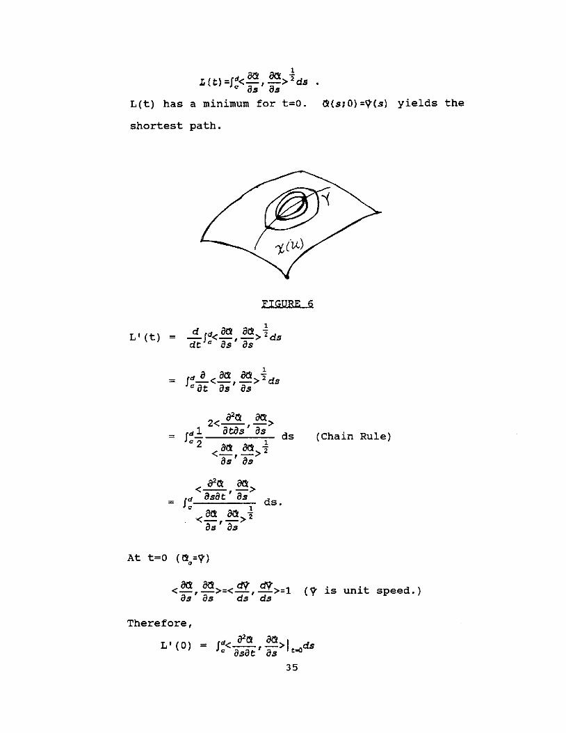
1

L(t)=fd<~, ~>2dS • c as as

L(t) has a minimum for t=o. ~(s;O)=?(s) yields the

shortest path.

FIGURE 6

L' (t)

2< (j2~ I act> fd.,!. atas as ds

c 2 1 <act, act>2

as as

(Chain Rule)

< O{t, ~>=< d?, d? >=1 (? is unit speed.) as as ds ds

Therefore,

L ' (0) = fd< cJ2~ ~>I d c osot I as t-o S

35

= Id[ d < act act> I _< act ~ct>1 ] ds c ds at' as t-O at' as 2 t-o

act I t-o=Ev j (s) Xj=A(S) S. "- was constructed so that at "-(c) = "-(d) = o. Therefore,

= - J""(s) kg(s) ds<O. (?"=k S+k if ) g II

This contradiction implies that the geodesic curvature

is everywhere 0 and ? is a geodesic. QED

The converse of the previous theorem is false:

If ~ is a geodesic, then ? is the shortest curve

between P and Q. A geodesic need not minimize distance.

Let P and Q be two points on the unit sphere S2 with

P + ±Q. There are two geodesics of different lengths

joining P to Q. They correspond to the two arcs of the

great circle through P and Q. The longer geodesic does

not minimize distance. However, geodesics locally

minimize length ..

36

4. Curvature.

An (n - 1) submanifold of an n-manifold is called a

hypersurface. Let M be a hypersurface of Rn, and let V be

the natural connection on Rn, and assume N is a unit normal

vector field that is C· on M. Thus <NpM,NpM> = 1 and

<NpM,X> = 0 for all P in M and X in TpM. Such an N always

exists locally.

For any P in M and any vector X in TpM, define the

linear map L: TpM - TpM by L(X) = VxN. The vector L(X) lies

in TpM. L is called the Weingarten map and in the case of

Rn, it has the geometric interpretation of the Jacobian of

the sphere map (Gauss map).

Let N=(al' ••• '~)' so the a i are real-valued C· functions

on M and L(ad 2 = 1. Then the mapping of g:M - Sn-1 in Rn is

a C- map of M into the unit (n-l) -sphere Sn-1. g is called

the sphere map (or Gauss map). If X is in TpM and act) is a

curve fitting X with a(O)=P and To(O)=X, then

g-(X) Tgoa(O) (xal , ••• ,xall

) VII L (X) •

FIGURE 7

37

The map L is c· on M in the sense that if X is c· on the

subset A of M, then L(X) (Xa l , ••• ,Xan ) is also C- on A

since each ai is C-on M. The Weingarten Map is the

derivative of the normal and therefore gives the change in

the normal.

In order to study how a two-dimensional manifold M

(simple surface) is curving at a point P, without reference

to a direction, find the eigenvalues of the matrix

(Lkl) = L (the Weingarten map). These eigenvalues at a

point P will tell us how M curves at that point.

4.1 Defjnjtjon. Let n be a unit normal vector on U.

The coeffjcjents of the second fundamental form of

a simple surface x :UcR2_R3 are the functions Lij

defined on U by Lij = <Xij ' n>.

Since Xij = Xjif then Lij = Lji . The Lij are called the

coefficients of the second fundamental form because the

assignment II (X, Y) = Li,j Lij xiyj is a symmetric bilinear

form on T~, as is the first fundamental form I(X,Y) =

<X, Y> = L xiyj <Xii Xj> = L xiyj gij.

4.2 Theorem. Let M be a surface. Then L is a linear

transformation from TpM to T~.

(See Millman and Parker, [9])

~ Theorem. Let M be a surface. If L(Xk) = L L/X1i

L/ = 1: Lik gil where (L/) is the matrix representing L with

respect to the basis {Xl 'X2 }.

Proof: Since Xi is tangent to M, <n,Xi> = o. This

38

implies that

o = < an X> <niX, .. > ::I ' 1 ..LA IIXJc

= -<L(Xk) ,Xi> + Lik = Lik - <L Lkj Xj,Xi>

= Lik - L Lkj <Xj,Xi> = Lik - L Lkj gji·

Therefore Lik = L Lkj gji and

L Lik gil = L Lkj gji gil = L Lkj 0/ = L/. QED

The normal curvature kn of a at P depends only on the

unit tangent of a at P. If we know all the possible values

that kn takes on at P, we would know how M curves at that

point. One way to find this information would be to find

the maximum and minimum values that kn obtains called

kl and k2' respectively. The following results are from

elementary linear algebra. (See ortega,[ll]) To find

these values, we determine the maximum and minimum of

II(X,X) as X runs over all unit vectors in TpM. This means

we are maximizing and minimizing II(X,X) subject to the

constraints <X,X> = 1.

Find the cri.tical values of

f(X,A) = II(X,X) - A«X,X> - 1)

= <L(X) ,X>' - A<X,X> + A = <L(X)-AX,X> + A at P.

The problem has a solution since II(X,X) does have a maximum

and minimum: the set of unit vectors in TpM is closed and

bounded, i.e., compact. The eigenvalues are the roots of

o = det(L - AI) = A2 - (trace L)A + det L.

Denotes these roots by kl and k2' with kl ~ k2•

39

4.4 Proposition. At each point of a surface M there

are two orthogonal directions such that the normal curvature

takes its maximum value in one direction and its minimum

value along the other. (See Ortega, [11])

4.5 Definition. The principal curvatures of a surface M

at a point P are the eigenvalues of L (k1 and k2) at

the point P. Corresponding unit eigenvectors are

called principal directions at P.

4.6 Definition. The Gaussian curvature of M at P is

K klk2 = det L. The mean curvature of M at P is

H = 1/2 (k1 + k 2 ) = 1/2 trace (L) .

In the previous examples of two-dimensional manifolds,

the geodesics of these surfaces were discussed. In each

case, the Weingarten map L and the curvature of these

surfaces can be computed.

4.7 Example. For the Euclidean plane x(r,s) = (r,s,O),

the metric coefficients were found to be

Therefore Lij = <Xij , Ii> = < (5, Ii> 0 for all i and j and

L =

The det L = ° and 1/2 trace(L) = 0. This implies that the

Gaussian and mean curvatures of the Euclidean plane at any

point P is 0.

4.8 Example. The unit sphere S2 - {0,0,±1} was given by

x(u,v) = (casu cosv,cosu sinv, sinu) , (u,v) E

40

The metric coefficients were given by

1 0 1 0 (gij) = ) with inverse (gij) = (0 1 (0 cos2u

cos2u

if = -(cosu cosv, cosu sinv, sinu} ,

Lll = 1, Ll2 = ~l = 0, and ~2 = cos2 u.

Therefore

1 0 L = (0 1) with det L = 1 and 1/2 trace(L) = 1.

The Gaussian and mean curvatures af the unit sphere 52 at

any point P is 1.

4.9 Example.

Let x(u,v) = (r casv casu, r casv sinu, rsinv) be

the sphere af radius r.

Xl = (-r casv sinu, r casv casu, 0)

X2 = (-r sinv casu, -r sinv sinu, r casv)

1

o

XII (-r cosv cosu, -r casv sinu, 0)

Xl2 = (r sinv sinu, -r sinv casu, 0)

X22 = (-r casv cosu, -r cosv sinu, -r sinv) X1xX2 if = (cosv cosu, cosv sinu, sinv)

IX1XX21

Lll = -r(cos2v), L12 = ~l = 0 , ~2 = -r

41

1

L = (L/) = L Likgil and L = r

o r

Therefore, det L = 1 and 1/2 trace (L) = -.! which yield r2 r the Gaussian and mean curvatures, respectively, of the

sphere at a given point p.

4.10 Example. For the circular cylinder

x(t,v) = (r cost, r sint, v) the metric coefficients are

1/r2 0 ) with inverse (gij ) = (

o o v' 2 o

) . 1/v'2

Let Ii = (cos t, sin t,O) with Lll -r, L12 = L2I =0, and

L22 = O. Therefore,

L = 1/r 0 1 o 0) with det L = 0 and 1/2 trace (L) = 2r'

It follows that the Gaussian curvature of the cylinder is

0, while the mean curvature is -.! . 2r

The above examples all had constant curvature ~ O.

Now we turn to an example with variable curvature:

positive, negati~e, and O.

4.11 Example. In studying the torus, we find that the

Gaussian curvature of a point P depends upon the point's

position on the surface. Let

x(u,v) =«a + b cosu)cosv,(a + b cosu)sinv, bsinu)

O<b<a, (u,v) E R X R. The metric coefficients are

o (a bcosu) 2

)

42

with inverse 1 0

(gij) b 2

1 ) .

0 (a bcosu) 2

n = -(cosu cosv, cosu sinv, sinu) and

Lll = b, L12 = L21 = 0, L22 = (a + bcosu) cosu.

Therefore 1 0 b

L = ) with 0 cosu

(a bcosu)

Det L = cosu which is b (a bcosu)

a) > 0 for ~<u< n 2 2

b) = o for u = ± n 2

n 3n c) < 0 for -<u<- . 2 2

These three cases represent the outside, the top and

bottom circle, and the inside respectively.

One of Gauss's deepest and most surprising observa-

tions in his investigation of curved surfaces is that the

curvature of a surface can be expressed in terms of its

metric and the derivatives of its component functions.

This metric is expressed in the form

Edx2 + 2 Fdxdy + Gdy2 where

E = <a/ax, a/ax>, F = <a/ax,a/ay>, G = <a/aY,a/ay>.

Gauss called this theorem "egregium" because it is so

remarkable. K is defined very extrinsically, in terms of

43

n or L, none of which are intrinsic. Yet K is intrinsic.

4.12 Theorem. Gauss's Theorema Egregium

The Gaussian curvature K of a surface is intrinsic.

(See McCleary, [8])

Stahl,[13], gives a version of the formula for finding

K as follows, where E.! = aE/ax, E2 = aE/ay, Ell = a2E/ax2,

etc.

4 (EG - F2) 2 K

= E[E2G2 2F1G2 (G1) 2] + F[E1G2 E2G1 2E2F2 4F1F2 2F1G1]

+ G [E1G1 2E1F2 (E2) 2] 2 (EG F2) [E22 2F 12' Gll].

This formula will be used to compute the Gaussian

curvature for some of the models of non-Euclidean

geometry discussed in chapter two.

44

5. cut Locus

Take two points P and Q of a connected Riemannian

manifold M and join them by a continuous piecewise

differentiable curve. We can measure the arc length of

this curve using the Riemannian metric. All possible

piecewise differentiable curves joining P and Q will be

considered. Define the distance d(P,Q) between P and Q

as the infimum of their arc lengths. The distance function

d satisfies the usual three axioms of a metric space:

(1) d(P,Q) = d(Q,P).

(2) For all points P and Q in S, d(P,Q) ~ 0

and d(P,Q) = 0 if and only if P = Q.

(3) (The triangle inequality). For all P, Q, and

R in the metric space d(P,Q) + d(Q,R) ~ d(P,R).

This allows us to talk about cauchy sequences of points of

M and also the completeness of M. A metric space is

complete if every Cauchy sequence of points in the space

converges to a point in the space.

Assume that M is a complete Riemannian manifold.

Since a compact. metric space is complete, a compact

Riemannian manifold is always complete. A geodesic get)

can be parametrized by arclength. A geodesic

get) defined on the interval astsb, is said to be

infinitely extendable if it can be extended to a

geodesic get) defined for th~ whole interval, -~<t<~.

5,1 Definition. A surface S is said to be geodesjcaJJy

45

complete if every geodesic g:[a,b]-S can be extended

to a geodesic g:R-S.

Take the Euclidean plane and delete the origin. This

yields an incomplete Riemannian manifold because the

positive x-axis is not infinitely extendable. The

following important theorem relates metric complete-

ness and geodesic completeness.

5.2 Theorem. (Hopf-Rinow) On a complete Riemannian

manifold, every geodesic is infinitely extendable and any

two points can be joined by a minimizing geodesic.

(see Mccleary, [8])

At each point P of a complete Riemannian manifold M,

define a mapping of the tangent space T~ at Ponto M as

follows. If X is a tangent vector at P, draw a geodesic

g(t) starting at P in the direction of X parametrized by

arclength. Parametrize the geodesic in such a way that

g(O)=P. If X has length a, then we map X onto the point

g(a) of the geodesic. Denote this mapping by expp:TpM-M. p

FIGURE 8

This mapping is called the exponentjal map at P. Expp maps

a line in the tangent space TpM through its origin onto the

46

geodesic of M through P in the direction of the line. Since

every point Q of M can be joined by a geodesic to P, expp

maps TpM onto M.

5.3 Definitjon. Fix a point P of a complete Riemannian

manifold M and a geodesic get) starting at P.

A cut point of P along get) is the first point Q

on get) such that, for any point R on get) beyond Q,

there is a geodesic from P to R shorter than g(t).

This implies that Q is the first point where get)

ceases to minimize distance (or arclength) .

Let A be the set of positive real numbers s such that

the geodesic g(t), o~t~s, is minimizing where s=d(P,g(s».

Either A=(O,oo) or A=(O,r) where r is some positive number.

If A=(O,r), then g(r) is the cut point of P along the

geodesic get). If A=(O,oo), then we say that P has no cut

point along the geodesic get). Therefore, if Q is a point

on get) which comes after the cut point pl=g(r), such that

Q=g(s) with s>r, then we can find a geodesic from P to Q

which is shorter .than get). If Q is a point which comes

before the cut point pi, then we cannot find a shorter

geodesic from"P"to Q and there is not another geodesic from

P to Q of the same length.

5.4 Theorem. If Q comes before pi, then get) is the

unique minimizing geodesic joining P and Q.

Proof: Let h(t) be another minimizing geodesic from

p to Q. By moving from P to Q along h(t) and

47

continuing from Q to pI along get), we obtain a

nongeodesic curve a from P to pI with an arclength

equal to the distance d(P,P').

Choose a point M on h(t) before Q and also a point

W on get) after Q. Taking M and W sufficiently close

to Q, replace the portion of a from M to W by the

minimizing geodesic from M to W. We obtain a curve

from P to pI with an arclength less than the distance

d(P,PI) which is impossible. QED

FIGURE 9

5.5 pefinition. The set of cut points of P is called the

cut locus of P and is denoted by C(P).

If M is a compact Riemannian manifold, then on each

geodesic starting from a point P, there is a cut point of P.

Let M be an n-dimensional unit sphere. As in the unit

sphere S2, the geodesics are the great circles. If P is the

north pole, then the cut locus C(P) reduces to the south

pole. The cut locus of a point P of a cylinder in R3 is

the opposite generator to that which passes through P.

However, there is a geodesic, namely, the generator through

P, that extends infinitely far.

48

6. Geodesic Circles, Normal Neighborhoods, and Conjugate Points

6.1 Pefinition. A region D is convex if any two points of

it can be joined by a geodesic arc lying wholly in D.

A convex region is called simple if there is not more

than one such geodesic arc. In the Euclidean plane,

every convex region is simple, but this is not so for

a surface in general. The surface of a sphere is

convex but not simple.

6,2 Theorem. (J.H.C. Whitehead (1932»

Every point P of a surface has a neighborhood which is

convex and simple and every point can be joined uniquely to

every other point.

A particular form of Whitehead's theorem is concerned

with a geodesic circle of given center P and radius r. This

geodesic circle (or geodesic disk) is defined as the set of

points Q such that there is a geodesic arc PQ of length not

greater than r. This geodesic circle and normal

neighborhood will be discussed in this section.

In this section, it will be shown that short enough

geodesic segments behave as well in an arbitrary geometric

surface as they do in R3. In the Euclidean plane, if we

are interested in the distance to the origin, we use polar

coordinates as a convenience. The distance from the origin

to the point l(u,v) = (u cosv, u sinv) is simply u. In R2,

the u-parameter curves are geodesics radiating out from some

49

fixed point P of M.

Such geodesics may be described as follows: If W is a

unit tangent vector at P, let Q'w be the unique geodesic

which starts at P with initial velocity W. Assembling all

these geodesics into a single mapping yields the following.

6.3 Definition. Let l,k be orthogonal unit vectors tangent

to M at P. Then x(u,v) = Q'cosvi + sinvk (u) is the geodesic

polar mapping of M with pole P.

The domain of x is the largest region of R2 on which

the formula makes sense. A choice of v fixes a unit tangent

vector W = cosvl + sinvk at P. Then the u-parameter curve

u-x(u,v) = Q'w(u) is the radial geodesic with initial

velocity W. Since Ilwl! = 1, this geodesic has unit speed, so

that the length of Q'w from P=Q'w(O) to Q'w(u) is just u. At

the origin of R2, the geodesic polar mapping becomes

x (u, v) = Q'cosvi + sinvk (u) = (5 + u (cosv 1 + sinv k)

= (u cosv,u sinv).

Therefore x is a generalization of polar coordinates in the

plane.

The pole P is a trouble spot for a geodesic polar

mapping. To clarify the situation near P, define a new

mapping

y(u,v) = Q'ui + vk (1).

Y is differentiable and regular at the origin. By the

inverse function theorem, y is a diffeomorphism of some

disc De: u2 + v2 < e:2 onto a neighborhood Ne of P. Ne is

50

called a normal neighborhood of P. In the special case M =

R2, Y is just the identity map y(u,v) = (u,v). Therefore

for arbitrary M, y is a generalization of the rectangular

coordinates of R2.

6.4 Lemma. For a sufficiently small number e: > 0, let

Ss be the strip O<u<e: in R2. Then a geodesic polar mapping

x:Ss - M with pole P parametrizes a normal neighborhood Ns

of P - omitting P itself.

:2.

1R

FIGURE 10

Proof: Note that x bears to y the usual relationship

of polar coordinates to rectangular coordinates. This

implies that

x (u,v) = CXcosvi + sinvk (u) = cxucosvi + usinvk(l)

= y(u cosv,u sinv).

This formula expresses x as the composition of two

regular mappings:

(1) The Euclidean polar mapping

(u,v) - (u cosv,u sinv)

which wraps the strip Sa around the disc Os, and

51

(2) The one-to-one mapping y of Os onto Ns •

Therefore x is regular and carries 5s in usual polar-

coordinate fashion onto the neighborhood Ns - omitting

only the pole. QED

A fundamental consequence of the previous lemma is that

if Q = x(uo,vo) is any point in a normal neighborhood Ns of

P, then there is only one unit speed geodesic from P to Q

which lies entirely in N, namely, the radial geodesic

cx(u) = x(u,vo), O~u~uo.

6,5 Example, Given the unit sphere 52, let P be the

north pole (0,0,1), The geographical parametrization

x(u,v) = (sinu cosv, sinu sinv, cos u)

yields the geodesics radiating out from P.

Each u-parameter curve is a unit-speed parametrization

of a great circle and is therefore a geodesic.

Xl = (cosu cosv, casu sinv,-sinu) and for u = 0,

Xl (O,v) = (cosv, sinv, 0) = cosvi + sinvk

with i=(l,O,O)P and k=(O,l,O)P.

By the uniqueness of geodesics,

x (u, v) = cxcosvi + sinvk (u) which shows that x as defined

above is the geodesic polar mapping of 52 with pole P.

Therefore the largest possible normal neighborhood Ns of P

occurs when e = IT, for on the strip 5n , X is a polar

parametrization of all the sphere except the north and south

poles.

6,6 Theorem, For each point Q in a normal neighborhood

52

Ng of P the radial geodesic segment in Ng from P to Q

uniquely minimizes arclength. (See O'Neill,[lO])

FIGURE 11

As a result of this theorem, if points P and Q are

close enough together, then as in Euclidean space, there is

a unique geodesic segment from P to Q which is shorter than

any other curve from P to Q. Unlike the Euclidean case,

there may be many other nonshortest geodesics from P to Q.

If x is a geodesic polar parametrization at P, we shall

call the v-parameter curve u=e, the geodesic circle of

radius e whose center is P. Cg consists of all points at a

distance e from P.

6.7 Example. ·On a sphere of radius r the geographical

parametrization would be

x(u,v) = (rsinu cosv, rsinu sinv, rcosu) with

P=(O,O,I) •

Xl = (rcosu cosv, rcosu sinv, -rsinu) and

XI(O,V) = (rcosv, rsin v, 0) = cosrvI + sinrvk.

53

Therefore it (u, v) =Q'cosrvi + sinrvk (u) and each point P of the

sphere of radius r has a normal neighborhood Ns when

e = rrr. This is all of the sphere except the point, -P,

antipodal to the pole P. Therefore, if two points P and

Q are not antipodal (Q + -P) then there is a unique shortest

curve a from P to Q. Intrinsic distance on the sphere is

given by the formula d(P,Q) = r8 where 8 (os8sn) is the

angle from P to Q in R3. If P and Q are not antipodal,

then d(P,Q) = L(a) = reo As Q moves toward the antipodal

point -P of P, by continuity d(P,-P) = rrr. Therefore no

geodesic segment a of length L(a) > rn can minimize arc

length between its endpoints.

The Gaussian curvature K=(det L) of a geometric

surface M affects the geodesics of the surface.

(See section four for Gaussian curvature.)

6.8 Definition. A geodesic segment a from P to Q locally

minimizes arclength from P to Q provided that for any

curve segment B from P to Q which is sufficiently near

(e-close) to a, then L(B) ~ L(a) where L(B) = d(P,Q) •

This local minimization is strict (or unique) provided

we get strictly inequality L(B) > L(a) unless B is a

reparametrization of a.

Think of Q' as an elastic string or rubber band which

is constrained to lie in M, is under tension, and has its

endpoints pinned down at P and Q. Because a is a geodesic,

it is in equilibrium. If it were not a geodesic, its

54

tension would pull it into a new shorter position. If

Q is pulled aside slightly to a new curve B and released,

will it return to its original position Q? If B is longer

than Q, then its tension will pull it back to Q.

The study of local minimization on two-dimensional

manifolds depends on the notion of conjugate points. If

Q is a unit-speed geodesic starting at P, then Q is a u-

parameter curve, v=vo' of a geodesic polar mapping x with

pole P.

x (u, v) = Qcosvi + sinvk (u) = (u cosv, u sinv).

G=<X2, X2>=U2 where X2 = (-u sinv, u COSY)

Therefore at u=O, G is zero but is nonzero immediately

thereafter.

6.9 Definition. A point Q(s) =x(s,vo)=(s cosvo's sinvo)

with s > 0 is a conjugate point of Q(O) = P on Q

prov ided G (s , v 0) = 0 where G=<X2, X2>=S2 .

mayor may not exist.)

(Such points

The geometric meaning of conjugacy rests on the

interpretion of iG = II x211 as the rate at which the radial

geodesic u-parameter curves are spreading apart. For fixed

e > 0, if JG is large, then the distance from x(u,v) to

x(u,v+e) is large. This means that the radial geodesics

are spreading rapidly. When JG is small, then the distance

from x(u,v) to x(u,v+e) is small. Therefore the radial

geodesics are pulling back together again. It follows that

when G vanishes at a conjugate point Q(Sl) = X(Sl,Vo), for

55

v near Yo, the u-parameter curves have all reached this same

point after traveling at unit speed the same distance Sl.

However, this meeting may not occur.

6.10 Example. The Euclidean plane gives the standard

rate at which radial geodesics spread apart. For

x(u,v) = (u COSy, u sinv) with X2=(-U sinv, u cosv) ,

then G=<X2, X2>= u2 and ,fG = u. Therefore G does not vanish

and there are no conjugate points in the Euclidean plane.

6.11 Example. The unit sphere S2 with P=(O,O,l), the

north pole, has parametrization

x(u,v) = (sinu COSY, sinu sinv, cos u).

Therefore, X2 = (-sinu sinv, sinu COSY, 0) and ,fG = sinu.

Since sinu < u for u > 0, the radial geodesics starting at

the north pole P of S2 spread less rapidly than in R2.

Since vG(n,r)=sinn=O, the radial geodesics all have their

first conjugate point after traveling a distance of n.

6.12 Example. Let x be a geodesic polar mapping defined

on a region where G > 0. Then y'G;;:;lIx2 11 satisfies the Jacobi

differential equation

(,fG)11 + K ,fG = 0 subject to the initial conditions

,fG(O,v) = 0, (y'G)tCo,v) = 1 for all v, where

(,fG) 1 = (ajG/au) and (,fG ) 11 = ca2,fG/au2) and

K = Gaussian curvature. The restriction G > ° is

needed to ensure that ,fG is differentiable. y'GCu,v) is

well-defined for u=o since .jGco,v) = IIX2(O,v) II = 0.

jG need not be differentiable at u = 0, so interpret

56

({Gh (O,v) and ({G )l1(O,V) as limits such as

({G ) 1 ( ° , v) = lim u-o (fG ) d u , v) .

For the Euclidean plane fG = u, {G(O,v) = ° and

({G)l(O,V) = 1 for all v. Therefore the initial conditions

show that as the radial geodesics leave the pole P in any

geometric surface, they are spreading at the same rate as

in the Euclidean plane. But the Jacobi equation shows that

immediately thereafter the rate of spreading depends on the

Gaussian curvature of the surface. For K < 0, radial

geodesics spread apart faster than in R2. For K > 0, the

rate of spreading is less than in R2.

In the Euclidean plane, we found the Gaussian curvature

to be zero. By measuring a short distance e in all

directions from P, we obtain the polar geodesic circle Cg

of radius e. The circumference of Cs is L(Cs ) = 2rre. For

K > 0, the radial geodesics from P are not spreading as

rapidly as in the Euclidean plane, so Cs will be shorter

than 2rre. This implies that geodesic circles on a surface

of positive curvature are always "too small". For K < ° the radial geodesics from P are spreading more rapidly than

in the Euclidean plane, and Cs will be longer than 2rre.

Therefore geodesic circles on a surface of negative

curvature are always "too large".

As a consequence of the theorem, we can find {G on a

geodesic a by solving the Jacobi equation on a, subject

to the given initial conditions. Let a be a unit-speed

57

geodesic starting at the point P in M. Let g(u) = (G(u,Vo )

be the unique solution of the Jacobi equation on a,

gil + K(a)g = 0 such that g(O) = 0, gl(O) = 1. Then the

first conjugate point of a(O) = P on a (if it exists) is

a(sl)' where Sl is the smallest positive number such that

6.13. Example. Let a be a unit speed geodesic starting

at any point P of the sphere of radius r. The Gaussian

curvature along this geodesic (great circle) is 1/r2. The

Jacobi equation for a is given

gl I + g/r2 = 0 which has the general solution

g(s) = A sin (sir) + B cos (sir).

The initial conditions g(O) = 0, gl(O) = 1, yield the

equation g(s) = r sin (sir). The first zero of this

function with Sl > 0 occurs at Sl = rrr. Therefore the

first conjugate point of a(O) =P on a is at the antipodal

point of P.

6.14 Example. Let a be a unit-speed parametrization

of the outer equa~or of a torus of revolution T. On a

the Gaussian curvature is

cos u with u = o. b(a+bcosu)

It follows that a has constant positive Gaussian curvature

1 The Jacobi equation for a is b(a+b)

gil + g o which has the general solution b(a+b)

58

g(s) = A sin s + B cos s ./b(a+b) /b (a+b)

Therefore the first conjugate point a(s1) of a(O) = P on

a will occur at exactly the same distance S1 along a as if

a were on a sphere with this curvature. The initial

conditions g(O)=O, gl(O)=l, yield the equation

g(s) = v'b(a+b)sin( s ). v'b (a+b)

The first zero of this function with S1 > 0 occurs at

S1 = IT Vb (a+b) •

6.]5 Corollary. There are no conjugate points on any

geodesic in a surface with curvature K s O. Hence every

geodesic segment on such a surface is locally minimizing.

Proof: Let a be a geodesic in M. since g(O)=O

and gl(O)=l, we have g(s) ~ 0 for s ~ 0 at least up to

the first conjugate point (if it exists). But KsO

implies that gl I = -Kg ~ 0, so gl is an increasing

function with gl~l. Therefore g(s) ~ s up to the first

conjugate point which can never occur. QED

FIGURE ]2

If a is a geodesic segment from P to Q such that there

59

are no conjugate points of P = aCe) on a, then a locally

minimizes arc length from P to Q. On the circular cylinder

with K=O, the helical geodesic a from P to Q, with Q

directly above P, is locally minimizing, but it is certainly

not minimizing. The straight line segment cr provides a much

shorter way to get from P to Q.

In Ordinary Differential Equations, we say that y(x)

oscjllates on the interval [c,~) if y is nonconstant and

has infinitely many zeros on [c,~). Equations of the

form y" + p(x)y = 0 are oscillatory. The Jacobi equation

is of this form. Therefore all solutions of the Jacobi

equation are oscillatory. (See Derrick and GrosSman,[2])

This implies that if K~e>o, i.e., if K is positive and

bounded away from 0, then there must be conjugate points.

60

7. Gauss-Bonnet Theorem.

A triangle in the plane is determined by three line

segments and the region they enclose. A triangle on a

surface is determined by three geodesic segments that

enclose a region and is called a geodesic triangle. Gauss

deduced some of the basic properties of geodesic triangles

including a general relation between area and angle sum.

If a region D is simply connected in a surface S, then

any closed curve in D can be contracted to a point without

leaving the region. From H. Hopf we know that the tangent

along a closed piecewise differentiable curve enclosing a

simply connected region turns through 2rr. L f ajkg(s)ds

represents the total geodesic curvature along a, the

boundary of the region D. fJD K dA represents the total

Gaussian curvature of D with dA the element of area of D.

7.1 Theorem. (Gauss-Bonnet) If D is a simply connected

region in a regular surface S bounded by a piecewise

differentiable c~rve a making exterior angles el, ... ,en at

the vertices of a, then

L Jaj kg(s)ds + ffD K dA = 2rr - L ejo

(See McCleary, [8]) This formula contains geodesic

curvature, Gaussian curvature, and exterior angles, mixing

up curves, angles, and areas into a remarkable relation.

Gauss's version of the Gauss-Bonnet theorem is

concerned with geodesic triangles. Let R = ~Bc be such a

61

triangle with sides given by geodesic segments. The

interior angles are given by L-A=n - eA, LB = n - ee, and

LC = n - ee' Therefore 2n - eA - ee - ee

= 2n + LA - n + LB - n + LC - n = LA + LB + LC - n.

Since geodesic curvature vanishes on geodesics, then:

7.2 CoroJJary. (Gauss) For a geodesic triangle ~BC

on a surface, ff~ K dA = <A + <B + <C - n.

(See McCleary, [8])

In the Euclidean plane, the Gaussian curvature (K) is

zero. Therefore <A + <B + <C = n, and the interior angle

sum of a triangle in the Euclidean plane is n.

On a surface of constant positive curvature, such as

the sphere, let C = JfAABC K dA = K -area (~BC) > o.

Therefore c = <A + <B + <C - n, and <A + <B + <C = n + c

with c > 0, and the interior angle sum of a triangle on a

surface of constant positive curvature is greater than n.

On a surface of constant negative curvature, let

d = J fAABC K dA = K -area (t.ABC) < O. Then d = <A + <B +<C

- n, <A + <B + <C = n + d with d < 0, and the interior angle

sum of a triangle on a surface of constant negative

curvature is less than n.

There are many generalizations of the Gauss-Bonnet

Theorem. In its simplest form it states that positive

curvature everywhere implies positive Euler characteristic.

The Euler characteristic of a surface M is the integer

X = F - E + V. Let M be a compact surface in R3. Suppose

62

M can be broken into regions bounded by polygons, each

region contained in a simply connected geodesic coordinate

patch, with the segments of the polygon being geodesics. V

equals the number of vertices, E the number of edges, and F

the number of faces or number of polygonally bounded

regions. This version of the Gauss-Bonnet Theorem relates

two seemingly unrelated quantities, curvature (a

differential geometric quantity) with the Euler

characteristic X (a topological or combinatorial quantity).

7.3 Theorem. (Gauss-Bonnet) If M is compact then

JJM K dA = 2rrx. (See Millman and Parker, [9])

63

1. BELTRAMI DI5K

CHAPTER 2

NON-EUCLIDEAN PLANE

The notion of an abstract surface frees us to seek

models of non-Euclidean geometry without the restriction of

finding a subset of a Euclidean space. A set with a system

of coordinates and a Riemannian metric determines a

geometric surface. The models of non-Euclidean geometry in

this chapter are due to E. Beltrami (1835-1906) and

J. Henri Poincare (1854-1912).

1.1 Definjtjon A function f:51-52 between surfaces 51 and

52 is a diffeomorphism if it is differentiable, one-to-

one, and onto, and has a differentiable inverse

function. Two surfaces 51 and 52 are said to be

diffeomorph~c if there is a diffeomorphism f:51-52.

1.2a Defjnjtion. An isometry f:M-N of surfaces is a

diffeomorphism such that

<v,w> = <f.(v),f.(ii) >

for any pair of tangent vectors v,ii to M.

l,2h Defjnjtjon, A mapping of surfaces f:M-N is conformal

provided there exists a real-valued function g>O

on M such that

64

<iI,v> = g(P)<I.(il),f.(v) >

for all tangent vectors il,v to M. The function g is

called the scale factor of f.

If f is a conformal mapping for which g has constant value

1, then f is a local isometry. A local isometry preserves

lengths of tangent vectors. Therefore distances and angles

are preserved. Otherwise a conformal mapping is a

generalized isometry in which angles are preserved but

in which lengths of tangent vectors need not be preserved.

At each point P of M the tangent vectors at P all have their

lengths stretched by the same factor.

Beltrami studied and sought local conditions on a pair

of surfaces, Sl and S2' that guarantee that there is a local

diffeomorphism of Sl-S2 such that geodesics on 8 1 are taken

to geodesics on S20 Beltrami solved the problem when one of

the surfaces is the Euclidean plane. He found conditions

for the existence of a mapping taking geodesics on a surface

S to straight lines in the plane. Such a mapping is called

a geodesic mappi~g.

~ Theorem (Beltrami 1865). If there is a geodesic mapping

from a surface S to the Euclidean plane, then the Gaussian

curvature of the surface S is constant. (See McCleary,[8])

In the case of the sphere, central projection takes

great circles to straight lines. To construct the

projection, fix the tangent plane at a point R on the sphere

and join a point P in the adjacent hemisphere to the center

65

of the sphere. Extend this segment to the tangent plane and

this is the image of the point P. Central projection is

defined on the open hemisphere with R as the center.

If R is taken to be the south pole, then

i(A,~) = (-COSA cot~, -sinA cot~, -1).

FIGURE 13

A great circle is determined by the intersection of the

sphere and a plane through the center of the sphere. The

image of the great circle under central projection is the

intersection of this plane with the tangent plane, and

therefore determines a line. This projection will be

important for models of non-Euclidean geometry, so consider

the inverse of central projection.

1.4 Proposjtj6n The inverse of central projection of the

lower hemisphere of a sphere of radius R centered at the

origin to the plane tangent to the south pole (O,O,-R) has

the form

66

FIGURE 14

Proof: Let Q=(u,v,-R) denote a point in the plane

tangent to the south pole and consider the line segment

in ]i3 joining Q to the origin. This line segment

passes through a point P on the sphere. write the

coordinates of the point x(u,v) = P = (r,s,t). The

linear dependence of OP and OQ implies that

(0,0,0) = OP X OQ = (-Rs-tv, Rr+tu, rv-su).

It follows that r tu tv =-ands=-. -R -R

R It follows that x(u,v)=(r,s,t) (U,V,-R). QED VR2+U 2+V 2

From the inyerse of the central projection we can endow

the plane with the geometry of the sphere by inducing a

Riemannian metric on ]i2 via the mapping X:R2~S2. since

the sphere is a surface in ]i3, compute directly X1=XQ

and

X =X • 2 v

XI---------R-------3 (R 2 +V 2 ,-Uv,Ru) and (R2+u2+v2) "2

As in Example 3.2 of Chapter 1, the standard classical

notation for the Riemannian metric of a Riemannian manifold

is given by:

ds2 = Edu2 + 2Fdudv + Gdv2

the element of arc length or the line element on S. The

coordinate vectors Xl' X2 determine the following line

element on the sphere and thus on the plane in the induced

metric: ds2 R2 (R2+V2)du 2-2uvdudv+(R2+u 2)dv2

(R2+U2+V2) 2

computing the curvature associated with the metric induced

by the central projection yields K(P) = for all P. This

was computed by using Gauss's Theorema Egregium, stahl's

formula for curvature, and many tedious calculations.

Beltrami observed that the above calculation depends

on R2 and not on R. He therefore replaced R with J=IR to

develop a model of non-Euclidean geometry. The

abstract surface is the interior of the disk of

radius R in R2 centered at (0,0) and given by

D={ (u, v) ER21 U2+v2<R2}.

The ljne element, or element of arc length, becomes

ds2 = _R2 (v 2-R2) du 2-2uvdudv+ (u 2-R2) dv2

(_R2+U2+v2) 2

68

(R2_V2)du2+2uvdudv+(R2_U2)dv2 (R2-U2-V2) 2

(Formula 1)

This formula determines a Riemannian metric on the given

abstract surface. Since R=J=iR, the curvature is -1 constant and equal to --. The local differential equations R2

satisfied by the geodesic mapping in Theorem 1.1 will

continue to hold since we have only changed the constant

R2. It follows that the geodesics on this abstract surface

are Euclidean line segments.

Now fix the value of R as 1. Our abstract surface is

the interior of the unit disk, denoted by

DB = {(u, v) E R21 u 2+v2<1 } .

This disk is called the Beltrami disk. Let R = 1 in

Formula 1. The metric for the Beltrami disk is then given by

dSB2 = (1-v 2 ) du 2 +2uvdudv+(1-u 2 ) dv 2

(1-u 2-v 2 }2

where B represents Beltrami. The curvature which is

constant becomes 2;:;2;:;-l. R2 1

Choose a convenient point in the Beltrami disk. When

u=O or v=o the middle term of dSB2 vanishes and so the

geodesics u-(u,vo) and v-(uo,v) are perpendicular to the

v-axis or u-axis, respectively. At the center of the disk

the axes themselves are perpendicular geodesics. Our

convenient point is the origin (0,0). To discuss distance

from (0,0) and Euclidean circles centered at (0,0) polar

coordinates on the Beltrami disk are convenient. Let

u=rcos8, v=rsin8, du=cos8dr-rsin8d8, dv=sin8dr+rcos8d8.

69

Rewriting dsB2 as

dsB2 = (1-u 2 -v 2 ) (du 2+dv2) + (udu+vdv) 2

(1-u 2-v 2 )2

and substituting yields

= (1-x 2 ) (dX2+X2d~)+X2dx2 =

(1-x2) 2

A Euclidean line segment through the origin in the Beltrami

model, which is a geodesic, has polar equation 6=60, a

constant. If 0=(0,0) and P=(rcos60,rsin60), then

d:r 2 dsa

2 = (1-x2) 2

and the distance in the Beltrami model, denoted by dB(O,P),

is given by

As r approaches 1 the distance goes to infinity. Therefore

Euclidean lines through the origin have infinite length.

70

2. Poincare Disk

One problem with the Beltrami disk is the

representation of angles - the rays may be Euclidean line

segments, but the angles can be far from their Euclidean

appearance in measure. Fix a Euclidean angle, say n 2

between two line segments and place this Euclidean figure at

different points in the Beltrami disk. The angle measure

depends on the position of the vertex. For example, away

from the u- and v-axes, the line segments u~(u,vo) and

v-(uo,v) cross at (uo,vo) in an angle determined by the <XI ,X2>

(1-u2-v2) 2

This next model of non-Euclidean geometry again has the

interior of a Euclidean disk as the underlying abstract

surface. In this model, angle measurement agrees with its

Euclidean measure. An orthographic projection is a mapping

for which all lines of projection are orthogonal to the

plane of projection.

2.1 Proposition .. Orthographic projection of the Beltrami

model to the lower hemisphere of the sphere of radius one

centered at (0', d, 1) is a conformal mapping.

Proof: Orthographic projection is given by mapping

the Beltrami disk into s2+(0,0,1),

(u,v) ~(U,V,1-Jl-u2-v2). - u - V Xl = (1, 0, ) and X2 = (O , 1, )

J1-U 2_V 2 ~1-u2-v2

ds2 = Edu2 + 2Fdudv + Gdv2

71

= (1-v 2 ) du 2 +2uvdudv+(1-u 2 ) dv 2

l-u 2-v2

Comparing this equation with the line element on the

Beltrami disk yields ds2 = (1-u 2-v 2 )ds; and the mapping

is conformal. QED

Orthographic projection takes the geodesics in the Beltrami

disk, Euclidean line segments, to semicircles on the sphere

that meet the equator at right angles.

Follow this mapping by stereographic projection from

the north pole to the plane that is tangent to the south

pole, which is a conformal mapping of a sphere. The image

point p* of a point P on the sphere is the point of

intersection of the straight line through the north pole and

P and the tangent plane at the south pole. In this way, the

whole sphere, except the north pole, is mapped onto the open

plane in a one-to-one fashion. The images of the circles

parallel to the equator are concentric circles with their

common center at the south pole. The images of the

meridians are straight lines through the south pole. The

projection of the north pole is the point at infinity.

The mapping is represented by

p* where

rand R are the distances from P and P*, respectively, to

the z-axis. By using the similar triangles in Figure 15,

R 2

r and R 2r

72

p* FIGURE 15

As a result of the two mappings, the lower hemisphere

of the unit sphere maps to the disk of radius 2, centered

at the origin,

O2 = {( x , y) I X2 + y2 < 4}.

A Riemannian metric is induced on this disk O2 , called the

Poincare disk, by transfering the Beltrami

metric from the Beltrami disk via the diffeo-

morphism given by. the composite of orthographic and

stereographic projection:

(u, v) ~ (u, v, l-Jl-u 2-v2 ) ~ (x, y, 0)

2u 2v where x- and y = 1+Jl-u 2-v2 1+Jl-u 2-v2

Let w = -Jl-u 2-v2 , then

(udu+vdv) 2

(1-u 2-v 2 )2

73

, x= 2u --, l-w

y = 2v 1-w

, dx = 2 (1-w)du+2udw I dy =

(1-w) 2

This allows us to write

ds 2 _ (1-u 2-v 2 ) (du 2+dv2 ) + (udu+vdv) 2 = B (1-u 2-v 2 ) 2

and -wdw=udu+vdv, we obtain

2 (1-w)dv+2vdw (1-W)2

since X2+y2_1 __ U2 +V 2 -1-- 2w(1-w) _ 2w th t' . d d , e me rlC ln uce

4 (1-w)2 (1-w)2 1-w

by the mapping on D2 takes the form dx 2+dy2 ds 2= __ ---:---::;.-:--_

R 2 2 (1- x +y ) 2

4 It can be shown that the Poincare disk has constant

Gaussian curvature K=-l as does the Beltrami disk.

(See McCleary, [8])

As a point (u,v) approaches the rim of the Poincare . X 2+y2

disk, that is, the circle u2 + v2 = 4, then (1 - 4)

approaches zero. Therefore rulers must shrink as they

approach the rim, so that the disk is bigger than

our Euclidean intuition may suggest. Let 0 be a

constant polar angle and compute the arc-length function

set) of the Euclidean line segment aCt) = (t coso,t sino),

o~t<2, which runs from the origin almost to the rim.

a'(t)=(coso,sino) and with the given Riemannian metric,

74

<al{t),al{t»~ = 1 Therefore, aCt) has hyperbolic

speed

J<cI ( t) ,cI ( t) > ~ = Iia I (t) II = 1

It follows that

s (t) = It dt =2tanh-1.!=log 2+t • o t 2 2 2-t 1--

4

As t approaches 2, arclength set) from the origin a(o) to

aCt) approaches infinity. This "short" segment ex actually

has infinite hyperbolic length.

When working in the Poincare disk, polar coordinates

are a natural choice. This allows the metric to depend only

on the distance to the origin. Let

x(u,v)=(u COSY, usinv), 0<u<2, with du 2+dv 2

2

X1=(cosv,sinv) and x2 =(-u sinv, u

It follows that

E = 1 2

F = 0, G = 2

(1-~)2 4

(1-~)2 4

COSY) •

(1-~)2 4

2.2 Definition. A Clairaut parametrizatjon x:UcR2-M

is a parametrization in which F=<Xl ,X2>=0 and

E=<Xl' Xl> and G=<X2' X2> depend only on Xl (the u-

parameter curves).

2.3 Lemma. If x is a Clairaut parametrization, then all

the xl=u-parameter curves of x are geodesics.

Proof: A regular curve ex in M is a geodesic if and

only if ex has constant speed and geodesic curvature

75

~=O. a has geodesic curvature 0 if and only if a'

and a" are always collinear. For a Clairaut .. -+ cPx parametrization we need to show that Xl and Xll=--ou 2

are collinear. Since Xl and X2 are orthogonal, this

is equivalent to ~"Xll=O.

0=g2= (Xl"Xl ) =2Xl'X12 and O=Fl = (Xl "X2 ) l=Xll"X2+Xl"X2l •

Therefore, X2"Xll=O and all the u-parameter curves of

X are geodesics. QED

The polar coordinate parametrization of the Poincare

disk, x(u,v)=(u COSY, u sinv), O<u<2, is a Clairaut

parametrization, by Definition 2.2. Therefore the

u-parameter curves, Euclidean lines through the origin,

are geodesics of the disk.

2.4 Theorem. A curve B(u)=x(u,v(u)), where x is a

Clairaut parametrization, is a geodesic if and only if dv tolE du [G./G-C2

The constant c is then the slant of B, i.e., in

combination with G it determines the angle L

at which the geodesic B is cutting across the

u-parameter streamlines of x. (See O'Neill,[lO])

pi

FIGURE 16

76

since x is a Clairaut parametrization, E and G depend only

on u. Therefore the formula for dv depends only on u. du

By the fundamental theorem of calculus, it can be written

in integral form as

Therefore, in our given parametrization of the Poincare

disk, S(u) = x(u, v(u» is a geodesic provided

dv du

= ta{i fG./G-C 2

= ±

To carry out the required the integration, set a u 2 a w = - (1 + -), where a = u 4 ~

It follows that dv = ± dw/du du ~1-,,2

Therefore v-vo=±cos-1 w, or

a u 2 = w = - (1+-).

u 4 Also

(*) 4u cos (v-vo) = o. a

FIGURE 17

using the law of cosines in the diagram yields the polar

equation of a circle of radius r, centered at x (u , v ) : Q Q

77

comparing this equation with (*) above shows that B is a

Euclidean circle with u;-r 2=4. since Uo > 2, the center

of the circle lies outside the Poincare disk: X2+y2<4.

Orthographic projection is a conformal mapping that takes

the geodesics in the Beltrami disk, Euclidean line segments,

to semicircles on the sphere that meet the equator at right

angles. Then stereographic projection, which is a conformal

mapping, takes the equator to the rim of the Poincare disk.

It follows that the semicircles on the sphere that meet the

equator at right angles are taken to arcs on the disk that

are orthogonal to the rim of the Poincare disk. Therefore

the Euclidean circle C is orthogonal to the rim of the

disk.

If follows that the geodesics of the Poincare disk

x2 + y2 < 4 are all Euclidean lines through the

origin, and all Euclidean circles orthogonal to the rim

of the disk.

The geodesic~ of the Poincare disk should be

compared to those of the Euclidean plane. Around 300 B.C.

Euclid established a set of axioms for the straight lines

of his plane. The goal was to derive its geometry from

axioms so reasonable as to be "self-evident". The most

famous of these is equivalent to the parallel postUlate:

If P is a point not on a line a, then there is a unique

line B through P which does not meet a.

78

Over time, this postulate began to seem less self-evident

than the others. The axiom that two points determine a

unique straight line can be checked by laying down a long

but finite straight edge touching both points. But to

check the parallel postulate, also called Euclid's V, one

would have to travel the whole infinite length of B to be

sure it never touches a.

Much effort was given to trying to deduce the parallel

postulate from the other axioms. The Poincare disk

offers convincing proof that this cannot be done.

If we replace "line" by "route of geodesic", then every

Euclidean axiom holds in the Poincare disk except the

parallel postulate.

FIGURE 18

Given two points one and only one geodesic route runs

through them. But, as Figure 18 shows, in the

Poincare disk there are always an infinite number of

geodesic routes through P that do not meet a. When the

implications of this discovery were worked out, the hope

of deducing the parallel postulate was destroyed. The

whole idea that R2 is, in some sense, an Absolute whose

79

properties are "self-evident" was also destroyed. ]l2

became but one geometric surface among infinitely many

others discovered by Riemann.

80

3. Poincare Half-Plane

A. Geodesics and Curvature

In 1882, Poincare used the methods of stereographic

and orthographic projection to provide another conformal

model of the non-Euclidean plane, the Poincare half-plane.

The Poincare half-plane can be constructed by projecting the

Beltrami disk orthographically to the lower hemisphere of

the sphere of radius one centered at (0,0,1). This

orthographic projection is a mapping DcR2 to the lower

hemisphere of S2 for which all lines of projection are

perpendicular to the plane containing DB (Beltrami disk).

This is accomplished by the mapping

(u,v) ~- (u,v,1-V1-u2-v2).

The sphere is then rotated around the axis through the

center parallel to the x-axis through a right angle to

move the lower hemisphere to the half-space y>o. The

lower hemisphere is now the "right hemisphere." This is

represented by the mapping

(u,v,1-Vl-u 2-v2) ~- (u,Jl-u 2-v 2 ,V+1).

Now stereographically project from the north pole. This

takes the new "right hemisphere" of the sphere to the

upper half-plane in a2 given by H ={(u,v) Iv>o}. This

stereographic projection is represented by the mapping 2u 2Jl-u 2 -v2

(u,y'1-u 2-v2,v+l) ~- ( , ) 2- {v+l) 2- (v+l)

81

The composite mapping of the Beltrami disk into the Poincare

half-plane is 1_ 2u 2.Jl-u 2-v 2

(u,v) r (--, ). l-v l-v

NP

FIGURE 19

To find the metric on the half-plane induced by this mapping

let 1 -2udu-2vdv 2 w -wdw=udu+vdv,

x =

dy =

2u --, l-v y = 2w --, l-v

2 (l-v) dw+2wdv (l-v) 2

dx = 2 (1-v)du+2udv and (l-v) 2

The Beltrami metr-ic can again be expressed as

dSs2 = J:... (du 2 +dv 2 +dw 2 ) and

w2 -- 4 dx2 + dy2 = (du 2 +dv 2 +dw 2 ) =

(l-v) 2

This equation yields the induced metric (called the Poincare

metric)

ds 2 = P

The Poincare half-plane represents the abstract surface with

82

the given induced Riemannian metric.

3.1 Proposition Let h be a Euclidean circle with center

C(c,O) and radius r. If P and Q are points of h such that

the radii CP and CQ make angles Q and B (Q<B), respectively,

with the positive x-axis, then the hyperbolic length of

arc PQ = In csc~-cot13

cscct-cotct Proof: Let t be the angle from the positive x-axis to

the radius through an arbitrary point (x,y) on h, then

x=c+rcost, y=rsint, dx=-rsintdt, and dy=rcostdt.

'I

(c.) 0)

FIGURE 20

Hyperbolic length of arc PQ =

Jdx 2 +dy 2 = I i (-rsintdt) 2+ (rcostdt) 2

I y. rsint

= I rdt ~sint

I · tdt-l cse~-eot13 = Mese - n • a cscct-cotct

QED

3.2 proposition. The hyperbolic length of the Euclidean

line segment joining the points P(a,Yl) and Q(a,Y2),

Proof: x=a constant and dx=O. The hyperbolic length

83

of PQ =

A geodesic segment in the Poincare half-plane is a

curve whose hyperbolic length is the shortest among all the

curves that join a given pair of points in the hyperbolic

plane.

3.3 Theorem The geodesic segments of the Poincare half-

plane are either

a) segments of Euclidean straight lines that are

perpendicular to the x-axis or

b) arcs of Euclidean semicircles that are centered on

the x-axis.

Proof: Let P(Xl,Yl) and Q(X2,Y2) be any two points of

the Poincare half-plane, and let h be a curve joining

them.

a) Case I: Xl = X2

In this case, the Euclidean line segment PQ is

perpendicular to the x-axis. Let the geodesic segment

h have equation x=f(y) and dxjdy is given by f' so

that dx=f'dy. The hyperbolic length of h is

I ..; (£/) 2dy 2Tdy2 Y

Y2 In Proposition 3.2, In -- was shown to be the Yl

hyperbolic length of the Euclidean line segment PQ

84

joining points P(a'Yl) and Q(a'Y2). This implies that

segments of Euclidean straight lines perpendicular to

the x-axis are geodesics of the Poincare half-plane.

b) Case II: x1 + x2

't

----->----~----S....-~----x C FIGURE 21

In this case, the Euclidean line segment PQ is not

perpendicular to the x-axis. Let C(c,O) be the x-

intercept of the perpendicular bisector to PQ. Place

a polar coordinate system so that its origin coincides

with C and its initial ray points in the same direction

as the positive x-axis. Let the geodesic segment h be

a part of the curve whose equation is r=f(e). Let

the coordinates of P and Q be (rp,a) and (rQ,B),

respectively. The hyperbolic length of h is

Relate these polar coordinates to the defining

Cartesian coordinates by the equations:

x = c + rcose, y = rsine.

It follows that

85

dx= dx cos6+r dcose -x'cos6-rsln6 and de de de

dy dx . 6 dslne ,. 6 6 -=-Sl.n +r -x Sl.n +rcos • de de de

dx2 + dy2 =

(r' cose - rsine) 2 de2 + (r' sine + rcose) 2 de2

= (r,2 + r2) de2•

It follows that

h idx2 +d y2 fh I (Xl) 2+X2 de

y rsln9

h R de f! csce de = In csci3-coti3 <:

xsin9 cscct-cotct

In Proposition 3.1 this expression was shown to be

the hyperbolic length of the arc of the Euclidean

circle with center C(c,O) and radii CP=CQ. It follows

that this arc is the geodesic segment joining P and Q

and that arcs of Euclidean semicircles with centers on

the x-axis are geodesic segments of the Poincare half-

plane. QED

3.4 Example Find the hyperbolic length of the geodesic

segment joining the points A(S,4) and B(O,S).

x S6

Find the intersection of the perpendicular bisector to

the Euclidean line segment AB with the x-axis. This gives

point C which is the center of the geodesic joining A and

B. The Euclidean straight line joining A and B has slope

4-8_~ and the midpoint M of the Euclidean line segment AB 8-0 2

has coordinates (0+8, 8+4)=(4,6). Therefore the 2 2

perpendicular bisector has equation y-6=2(x-4) and the

x-intercept is (1,0). CA=CB=J(8-1)2+(4-0)2=yb5. It follows

that the hyperbolic length of the geodesic segment from A

to B is

In csci3-coti3 = In csca-cota

Consider the

E-2 4 4

Poincare metric

:::; 1. 45.

dx 2+dy2 y2

Using stahl's

formula for Gaussian curvature yields the following: 1 E=-

2 ' Y

-2 F2=0, G2= -3 '

Y

4 (~-O) 2K = y4

1 4 1 4 1 6 - (-) +- (-) -2 (-) (-» ; y2 y6 y2 y6 y4 y4

4K -4 4K=-4 i and K=-1.

Therefore the Poincare half-plane with the given Poincare

metric has constant curvature K=-l. By Corollary 6.15,

there are no conjugate points an any geodesic in a surface

with Gaussian curvature K~O. Hence every geodesic segment

on such a surface is locally minimizing and the circum-

ference of the polar geodesic circle will be longer than

2rre for a given e>O, e small.

87

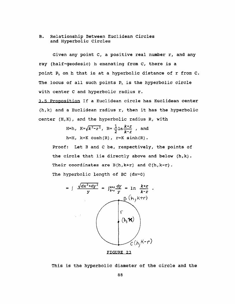
B. Relationship Between Euclidean Circles and Hyperbolic Circles

Given any point C, a positive real number r, and any

ray (half-geodesic) h emanating from C, there is a

point Ph on h that is at a hyperbolic distance of r from C.

The locus of all such points Ph is the hyperbolic circle

with center C and hyperbolic radius r.

3,5 Proposition If a Euclidean circle has Euclidean center

(h,k) and a Euclidean radius r, then it has the hyperbolic

center (H,K), and the hyperbolic radius R, with

H=h, K=·lk 2-r 2 R= lIn k+r and Y , 2 k-r'

h=H, k=K cosh(R), r=K sinh(R).

Proof: Let Band C be, respectively, the points of

the circle that lie directly above and below (h,k).

Their coordinates are B(h,k+r) and C(h,k-r).

The hyperbolic length of BC (dx=O)

= f JX+X dy = In k+r x-x y k-r

~-..::::e> Ch) k+r)

FIGURE 23

This is the hyperbolic diameter of the circle and the

88

h b 1 · d' 11 k+r h' h th yper 0 1C ra 1US R = - n---. H= S1nce x= on e 2 k-r Euclidean line segment perpendicular to the x-axis at

h. (H,K) should be the hyperbolic midpoint of segment

BC. By Proposition 3.2 of chapter 2, the hyperbolic

length of the Euclidean line segment joining points

(h,k+r) and (h,K)=(H,K) is In k+r and the hyperbolic K

length of the Euclidean line segment joining the points K (h,K)=(H,K) and (h,k-r) is In---. For (H,K)=(h,K) to k-r

be the hyperbolic midpoint of segment BC, then

k+r K ,....--;::--,.. In ---=In--- and K2;k2-r2,K;';k2-r2 • K k-r

When R= .!In k+r is inverted it yields 2 k-r

equations simultaneously, then K2

r2_ _K2sinh2 (R) and r;Ksinb (R) • coth2 (R) -1

and k=Kcosh(R). QED

3,6 coroJJary .Every Euclidean circle in the upper half-

plane is a hyperbolic circle. Every hyperbolic circle is

also a Euclidean circle.

C. Rigid Motions

3,7 Definition A mapping f:R4~R4 is an isometry if, for

89

The notion of isometry makes precise the ideas of

rigid motions and congruence. We define a congruence to

be a self-isometry of a surface, ~:S-S. Two figures, that

is subsets of S, are congruent if there is an isometry with

~(figurel) = figure2 • A figure made up of segments of

curves on a surface may be thought of as rods in a

configuration and the term rigid motion is synonymous with

congruence. Therefore, a rigid motion is considered to be

a transformation of a surface that does not distort its

configurations.

In Euclidean plane geometry, two triangles are

congruent if there is a rigid motion of the plane which

carries one triangle exactly onto the other. For these

congruent triangles, corresponding angles and corresponding

sides are congruent and the areas enclosed are equal. Any

geometric property of a given triangle is shared by every

congruent triangle.

3,8 Example A translation of R3 is an isometry. Fix a

point A in R3 and let T be the mapping that adds A to every

point of R3. Therefore, T(P)=P+A for all points P. T is

called transla.tion by A. T is an isometry since

~T(P)-T(Q)~=~(P+A)-(Q+A)~=~P-Q~.

3.9 Example In R2 the rotations given by

cose -sine La (v) = (sine cose)

in the standard basis are isometries.

90

II Lav11 2 =11 (COsev1-sinev2 , sinev1 +COSeV2 ) 112

= cos2 ev;-2 cos6sin6v 1 V2 +sin26v;+sin26v; +2 cosesinev 1 V2 +COS2eV22

= v;+v;=11 VIj2 • 3.10 Thegrem If F and G are isometries of RA , then the

composite mapping GF is also an isometry of RA.

Proof: Since G is an isometry, IIG(F(P) )-G(F(Q» II = II F (P) -F (Q) II. Since F is an isometry II F (P) -F (Q) II = II P-Q II • Therefore GF is also an isometry. QED

The rigid motions (isometries) of Euclidean and

hyperbolic space have formulations in terms of complex

numbers. The Poincare metric brought to light the role

played by complex numbers in this and other geometries.

Many mathematicians have come to think of the points of

the Poincare half-plane as complex numbers z=x+yi with a

positive imaginary part.

If c is any fixed complex number, then the function

f(z)=z+c is a translation of the Euclidean plane and every

translation of the plane is expressible in this manner.

For any angle Q and any complex number c, the function

f(z)=eiCl(z-c)+c = eiClz + (l-eiCl )c

is the rotation· about c, Rc,Cl where e iCl = COSQ +isinQ.

The 90° counterclockwise rotation of the plane about the

point (0,1) has the expression

Ri ,nl2 = e i (nIZ) (z-i) +i = i (z-i) +i = iz+1+i

in terms of complex numbers. If m is any line with

inclination Q to the positive x-axis, and c is a point on

91

m, then the function f(z)=e2ia z-c + c is the reflection

in the line m where z=x-yi is the conjugate of z=x+yi.

3,11 Theorem The rigid motions of the Euclidean plane

all have the form

f (z) =eiaz+c or f (z) =eia z+c

where a is an arbitrary real number and c is an arbitrary

complex number. Conversely, every function of either of

these forms is a rigid motion of the Euclidean plane.

(See Stahl, [13])

This leads us to the complex description of the rigid

motions of the hyperbolic half-plane. Horizontal transla-

tions and reflections in vertical lines, which are

geodesics, are also Euclidean rigid motions. They can be

expressed as f(z)=z+r or f(z)=-z + r, respectively, where

r is an arbitrary real number. A hyperbolic reflection is

either a Euclidean reflection in vertical lines, which are

geodesics, or an inversion centered at some point on the

x-axis.

3,12 Theorem The following transformations of the

hyperbolic plane preserve both hyperbolic lengths and

measures of angles:

a) inversions Ic,k where C is the center of a circle

on the x-axis and k is the radius;

b) reflections am where m is perpendicular to the

x-axis;

c) translations LM where AB is a Euclidean segment

92

parallel to the x-axis.

Proof: Inversions of the form Ie, k are conformal

transformations of the plane. Therefore Euclidean

measures of angles are preserved. The hyperbolic

measure of an angle coincides with its Euclidean

measure, and inversions of the form Ic,k preserve

hyperbolic measures of angles. Place a

polar coordinate system with its origin at C and

its initial ray along the positive x-axis. Let

h denote the curve r=f(e), C(~e~B. The inversion Ic,k k 2

maps h to h I given by r=F (e) = --, C(~e~B. fee) As in the proof of Theorem 3.3, the hyperbolic length

of hi is i (Xl) 2+X2 h. - de = xsine

"(x!) 2+X2 de = xsine

de

hyperbolic length of h.

It follows "that the given inversion does preserve

hyperbolic lengths and hyperbolic measures of angles.

For the proofs of parts b & c, see stahl, [13]. QED

I C • k represents an inversion whose fixed points are

exactly those that makeup the circle centered at C with

radius k. Euclidean reflections are defined so that their

93

axes are perpendicular bisectors of the line segment joining

any point to its image.

M FIGURE 24

Consider the reflection om whose axis is the vertical

line m, a geodesic, which is above the point M on the x-

axis. If P is any point of the upper half-plane, let h be

the geodesic through P that is an arc of a semicircle

centered at M. Since hand m are orthogonal at their

intersection A, it follows that om(h)=h and so P'=om(P) is

also on h. am is a hyperbolic rigid motion (as well as a

Euclidean rigid motion), and so the geodesic segments PA and

PiA have equal hyperbolic lengths. Therefore, m is the

hyperbolic perpendicular bisector of the geodesic segment h

joining P to its image P'=om(P).

Next look at the hyperbolic reflection that consists

of the inversion Ic,k where C is some point on the x-axis.

This inversion fixes every point on the geodesic n through

B which is an arc of a semicircle centered at C with radius

k. Therefore think of the geodesic n as the axis of Ic,k.

94

For any point Q between the x-axis and the geodesic n, let

Q' =Ic,k (Q) and let w be the geodesic that contains Q and is

orthogonal to n at their intersection B.

( FIGlffiE 25

It follows that Ie, k (w) =W and so Q' too is on w. Ie, k is a

hyperbolic rigid motion and so the geodesic segments QB and

Q'B have equal hyperbolic lengths. Thus n is the hyperbolic

perpendicular bisector of the geodesic segment joining Q to

its image Q'=Ie,dQ). Therefore hyperbolic reflections

satisfy the definition of reflections for Euclidean motions.

3,13 Proposition

FIGURE 26

Let m and n be two Euclidean lines

95

(geodesics) that intersect at a point A, and let a be the

counterclockwise angle from m to n at A. Then (In°(Jm = RA,2a'

(See Stahl, [13], and Figure 26)

Since hyperbolic reflections satisfy the definition

of reflections for Euclidean motions, this proposition

implies that the composition of two hyperbolic reflections

with intersecting axes is a hyperbolic rotation. The center

of this rotation is the intersection of the axes and the

angle of the rotation is twice the angle between the axes.

3.14 Theorem Every Euclidean rigid motion is the

composition of at most three reflections. (See Stahl, [13])

Since hyperbolic reflections satisfy the definition of

reflections for Euclidean motions, the following theorem

is implied.

3.15 Theorem Every hyperbolic rigid motion is the

composition of at most three hyperbolic reflections.

3.16 Example In the geodesic which is the arc of a

semicircle with center A=(a,O) on the x-axis and radius k,

the inversion IA,k(z) is given by . k 2

lA, k (z) = -=-- +a • z-a

k 2 If A=(O, 0), then Io,k(z)= -=-. The inversion Io,2 has the

z expression ~ and so it maps the point l+i to the point

2 z 2 4 . ( . ) ~:---= 2+21. See F1gure 27

l+i 1-i

42 3z+7 If A={3, 0), then I A,4 has the expression --+3 = %"-3 %"-3

-17+16i and so it maps l+i to the point (See Figure 5

96

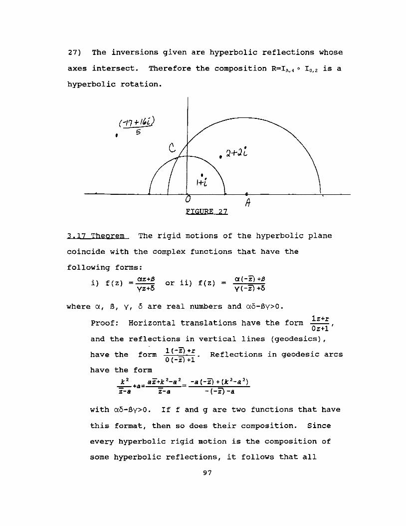
27) The inversions given are hyperbolic reflections whose

axes intersect. Therefore the composition R=IA,4 0 IO,2 is a

hyperbolic rotation •

•

• I+i o FIGURE 27

3.17 Theorem The rigid motions of the hyperbolic plane

coincide with the complex functions that have the

following forms:

i) f ( ) - ctz+13 z - yz+<S

or ii) f(z) = ct(-Z) +13 y( -Z) +<5

where a, B, V, 0 are real numbers and ao-Bv>O.

Proof: Horizontal translations have the form lz+,r --, Oz+l

and the reflections in vertical lines (geodesics),

have the form

have the form

1(-Z)+,r O(-Z)+l'

Reflections in geodesic arcs

k 2 aZ+k2-a 2 -=-+a---=,.----a (-Z) + (k 2 -a 2)

z-a z-a - (-Z)-a

with ao-Bv>O. If f and g are two functions that have

this format, then so does their composition. since

every hyperbolic rigid motion is the composition of

some hyperbolic reflections, it follows that all

97

hyperbolic rigid motions have either form i) or

form ii). QED az+b Transformations of the type f(z)=---- where a,b,c,d cz+d

are allowed to be any complex numbers as long as ad-bc+O,

are called Moebius transformations. If zo=a+bi is any

point of the half-plane, then the Moebius transformation z-a . f (z) = --- ~s a hyperbolic translation that carries Zo to b

i, and its inverse f-1(z)=bz+a carries i to zoo Therefore,

given any other point zl=c+di of the half-plane, the

composition z-a dz+(bc-ad) d( -- )+c = b Oz+b

is a hyperbolic rigid motion that carries Zo onto Zl. If

b=d, then this is a horizontal Euclidean translation. If

Zo=2-3i and zl=3+4i, then 4z+ (-3-3-2'4) _ 4z+17 is a --~--~3~--- -3

hyperbolic rigid motion that carries Zo onto Zl. Hyperbolic

rotations are characterized by a single fixed point in the

half-plane. To find the rotation, find the center and

locate the image of one other point .

3.18 Example

. l..

~/~

o FIGURE 28

Let f(Z)=2=Oz-1. z 1z+0

and this rotation is pivoted at i.

98

. f') -1 . Let Z=L (~=-=~ 1

. -1 1 f (2~) = -=- and it 2i 2

follows that the angle of rotation is 180°. Therefore

fez) is a Moebius transformation that is the hyperbolic

rotation by 180° about the point i. (See Figure 28)

D. Geodesic Triangles

3.]9 Definition A hyperboljc triangle ABC consists of

three points A,B,C (vertices) that do not lie on a

single geodesic and the three geodesic segments (sides)

that join each pair of vertices. A hyperbolic triangle

is said to be in standard position if the vertices

A,B,C have coordinates (O,k), (s,t), (0,1),

respectively, where k>l and s>O.

3.20 Proposjtjon Every hyperbolic triangle can be

brought into standard position by a hyperbolic rigid

motion.

Proof: Let the hyperbolic triangle ABC have its

vertices C at (0,1) and B at (s,t) with s>O, but

A is at (O,k) with k<l. Let z=ci with c<l. The

reflection I a,l= k~ = 1_=_1_=..!>1 will transform Z ci -ci c

triangle ABC into triangle A'B'C' that is in

standard position. (See Figure 29)

If the hyperbolic triangle ABC has both of its

vertices A(O,a) and C(O,c) on the y-axis, then by

reflecting this triangle in the y-axis, if necessary,

then B (s, t) has s>o. The reflection Io,.;c transforms

triangle ABC into a triangle in standard position

99

where

E FIGURE 29

If the hyperbolic triangle ABC is in an arbitrary

position, assume that its side AC is a segment of

a geodesic arc g that joins two points D and E on the

x-axis. Horizontal translations are hyperbolic rigid

motions. This allows us to assume that E is at the

origin. If D=(d,O) then the inversion ID,d transforms

g onto the y-axis where

k 2 ID,d = -=--+D =

z-D d 2

-=--+D z-D

The given triangle is transformed into triangle A'B'C'

which has one of its sides on the y-axis. By the

previous steps in this proof, triangle A'B'C' can be

brought into standard position. (See Figure 29) QED

3,21 Proposition At any given point P, let g be a

vertical geodesic ray and let gl' g2' g3 be geodesic arcs

centered at el , e2 , e3 respectively. Then

L (g, gl) ;LDC1P, L (gl' g2) =LC1PC2 , and L (g3' gl) =n-cl Pc3 •

100

D

" D FIGURE 30

I

x

Proof: Let 0' be a point of g such that P is between

o and 0'. Let PT1 and PT2 be the Euclidean tangent

lines to gl and g2, respectively, at P. since the

tangent to a circle is perpendicular to the radius at

the point of contact, then

B = L (gl,g2) = LT1PT2 = LT1PC1-LT2PC1

II = 2'-Li'2PCl = LT2PC2 -LT2PC1 = LC1PC2;

ex = L(g,gIl = LO'PT1 = II - LT1PC1 - LC1PO II = --LC PD = LDC1P; 2 1

Y = L (g3,gd = L (g),g) + L (g,gl)

The Poincare half-plane has constant curvature

K=-1. By the Gauss-Bonnet Theorem and its corollaries,

the interior angle sum of a triangle in the Poincare half-

plane is less than II. This is the only constraint on the

angles of the hyperbolic triangle. The next theorem's proof

contains a blueprint for the construction of hyperbolic

triangles with specified angles such that ex+B+Y<II.

101

3.22 Theorem Given any three angles whose sum is less

than rr, they are indeed the angles of some hyperbolic

triangle.

Proof: Let a, B, y be three arbitrary positive angles

such that a+B+y<rr. Let triangle ABC be a hyperbolic

triangle in standard position such that LCAB=a,

LABC=B, and LBCA=y.

o FIGURE 31

o.(u,o) x

Let G(u,O) and H(-v,O) be the Euclidean centers of

the geodesic arcs BC and AB, respectively. Let r

and s be their respective Euclidean radii. LCGO=y,

LOHA=a, LHBG~B by proposition 3.21. The trigonometry

of the Euclidean triangles GCO, AHO, and BGH yields

the constraints:

(1) u rcosy

(2) v = scosa

(3) (U+V)2 = r2 + S2 - 2rscosB.

By the Pythagorean Theorem r 2=u2+1. Along with (1)

102

it follows that

r = cscy and u = coty.

Substitute u, r, and v in (3) to get

(cotY+SCOS~)2 = csc2y + S2 - 2scosBcscy

which simplifies to the quadratic equation

(4) s2sin2~ - 2s(cos~coty + cosBcscy) + 1 = o. It follows that if triangle ABC is a hyperbolic

triangle in standard position that satisfies these

constraints, then its angles are indeed ~,B,y. The

quadratic equation (4) has discriminant

4(cos~coty + cosBcscy)2 - 4sin2~.

If this discriminant is necessarily positive, this

guarantees that the quadratic equation (4) does have

solution in s. Since ~+B+y<rr, then ~+y<rr-B. The

cosine function is monotone decreasing in the first

two quadrants. Therefore we have the following

sequence of equivalent statements:

cos(~+y) > cos (rr-B) = -cosB,

cos~cosy - sin~siny > -cosS,

cos~cosy + cosB > sin~siny > 0,

cos~coty + cosBcscy > sin~ > 0,

(cos~coty + cosBcscy)2 > sin2~.

The last inequality establishes the positivity of

the discriminant of (4). It follows that this

quadratic has two real solutions for any given

positive angles ~,S,y such that ~+B+y<rr. If

103

v=scosa, then s, v, u=coty, and r=cscy satisfy

equations (1), (2), and (3) and so the given

hyperbolic triangle does exist. QED

3,23 Example

1) Construct a hyperbolic triangle in standard position

with given angles: a=30°, B=50°, y=60°.

r=cscy=1.1547, u=rcosy=0.57735;

s2sin2a-2s(cosacoty+cosBcscy)+1=0 yields

s2(.25)-2s(1.2422)+1=0 and s= 2.4844±t5.1702. 0.5

sz9.52 or szO.421. Let sz9.52, then

v=scosa=8.244 and k=ssina=4.76.

FIGURE 32

2) Construct a hyperbolic triangle in standard position

with the given angles: a=60°, B=50°, y=30°,

u=rcosy=1.73 , r=cscy=2, s2(.75)-2s(2.152)+1=0,

and S = 4.304±t15.52 . 1.5

sz5.5 or szO.24.

Let sz5.5, then v=scosa=2.75 and k=ssina=4.76.

104

FIGURE 33

3) Construct a hyperbolic triangle in standard position

with the given angles: a=B=y=SO°.

r=cscy=1.30S, u=rcosy=0.839, s2(0.S87)-2S(1.378)+1=0,

and S= 2.756±~ • ----- s~4.3 or s~0.396. 1.174

Let s~4.3, then v=scosa=2.76 and k=ssina=3.29

FIGURE 34

In each of the three constructions, the hyperbolic

lengths of the sides of the triangles were found using

Propositon 3.1, Proposition 3.2, and Example 3.4 of this

chapter as well as the hyperbolic trigonometric formula~

105

sincx _ sin.B = siny sinha sinhb sinha

Let triangle ABC be any hyperbolic triangle with angles

a, S, and y with LCAB=a, LABC=S, and LBCA=y. Place this

triangle in standard positon, and let rand s be as in the

previous constructions. C and A have coordinates (0,1) and

(O,s sinal respectively. By Proposition 3.2 of this

chapter, the hyperbolic length of the side AC is

Iln(s sinal I. s was found by solving the quadratic

equation as in the previous constructions. It would seem

possible that there would be two triangles in standard

position determined by these angles. But there is only

one. Let Sl and S2 denote the two possible values of s.

since these are the roots of the quadratic equation (4)

in Theorem 3.22, it follows that

s s - 1 and therefore s2sinct= ~ . 1 2 sin2ct sl s~net

However, Iln~1 = lIn xl and so the length of side AC as X

given by lIn (s sina) I is completely determined by the

angles a, S, and y. This argument could have been applied

to any side of the hyperbolic triangle ABC. It follows

that every hyperbolic triangle is completely determined

by its angles.

3.24. Theorem. If two hyperbolic triangles have their

respective angles equal, then they are hyperbolically

congruent.

Generally speaking, a Euclidean triangle is completely

106

determined by any of its three sides and three angles. An

exception to this rule is the fact that a Euclidean triangle

is determined only up to similarity when only its three

angles are given. In the hyperbolic plane, this exception

does not occur and a triangle is completely determined

by its angles. In construction (3), a=B=y=50°. The

hyperbolic length of each side of the hyperbolic triangle

was found to be approximately 1.19. This will be true for

every hyperbolic triangle with a=B=y=50°. Therefore, in

the hyperbolic plane, similar triangles are congruent!

So if you lived in a 30°-30°-30° triangular house in

hyperbolic space, you could buy carpet and furniture

custom made to fit.

107

BIBLIOGRAPHY

[1] Chern, 5.5., MAA studies in Mathematics- studjes in Global Geometry and Analysis, New Jersey: Prentice-Hall, 1967.

[2] Derrick, William R. and Grossman, Stanley I., Introductjon to Differential Egyatjons with Boundary value Problems, st. Paul, Minnesota: West Publishing Company, 1987.

[3] Do Carmo, Manfredo Perdigao, Riemannian Geometry, Boston, Massachusetts: Birkhauser, 1992.

[4] Hicks, Noel J., Notes on Differential Geometry, New Jersey: D. Van Nostrand Co., Inc., 1965.

[5] Hsiung, Chuan-Chih, A First Course jn Differential Geometry, New York: John Wiley & Sons, 1981.

[6] Klingenberg, Wilhelm, A Course jn Differential Geometry, New York: Springer-Verlag, 1978.

[7] Kreyszig, Erwin, Introduction to Differentjal Geometry and Riemannian Geometry, Great Britain: University of Toronto Press, 1968.

[8] McCleary, John, Geometry From a Differentiable Viewpoint, New York: cambridge University Press, 1994.

[9] Millman, Richard S. and Parker, George D., Elements of Differential Geometry, New Jersey: Prentice-Hall, 1977.

[10] O'Neill, Barrett, Elementary Differentjal Geometry, New York: Academic Press, 1966.

[11] Ortega, James M., Matrix Theory, New York: Plenum Press, 1987.

[12] Spivak, Michael, A Comprehensive Introduction to Differential Geometry, Volume Two, Massachusetts: Publish or Perish, Inc., 1970.

108

[13J Stahl, Saul, The pojncare Half-plane: A Gateway to Modern GeomethY, London: Jones and Bartlett Publishers, 1993.

[14J Struik, Dirk J., Lectures on Classjcal Djfferentjal Geometry, Massachusetts: Addison-Wesley Publishing Company, Inc., 1950.

[15J Willmore, T.J., An Introduction to Differentjal GeomethY, Great Britain: Oxford University Press, 1959.

109

VITA

Name of Author: Deborah F. Logan

Place of Birth:

Date of Birth:

EDUCATION

M.S. in Mathematical Sciences, 1995 University of North Florida, Jacksonville, Florida

B.S. in Secondary Education, 1975 Mathematics Proficiency Tennessee Temple University, Chattanooga, Tennessee

TEACHING EXPERIENCE

1990-Present Adjunct Professor of Mathematics Florida Community college at Jacksonville South Campus and Kent Campus

Mathematics Instructor, 1976-1990 various high schools in Spartanburg, South Carolina Riverview, Florida Jacksonville, Florida

110