ITERATED INDEX FORMULAE FOR

CLOSED GEODESICS WITH APPLICATIONS*

Chun-gen Liu1

Department of Mathematics, Nankai UniversityTianjin 300071, People’s Republic of China

(e-mail: liucg@nankai.edu.cn)

Yiming Long2

Nankai Institute of Mathematics,Nankai University

Tianjin 300071, People’s Republic of China(e-mail: longym@nankai.edu.cn)

Abstract. In this paper, various precise iteration equalities and inequalities of Morseindices for the closed geodesics are established. As applications of these formulae,multiplicity results of closed geodesics on some Riemannian manifolds are proved.

1991 Mathematics Subject Classification. 58E05. 53C22, 58E10.Key words and phrases. Riemannian manifold, Morse index, iteration..1 Project 10071040 supported by NNSF, 200014 supported by Exc. Ph.D. Funds of ME of China,

and PMC key Lab. of ME of China.2 Partially supported by the 973 Program of STM, RFDP, MCME of China, CEC of Tianjin, S.

S. Chern Foundation, and PMC key Lab. of ME of China.

*Published in“Science in China”(2002)vol.45 No.1 (9-28).

Typeset by AMS-TEX

1

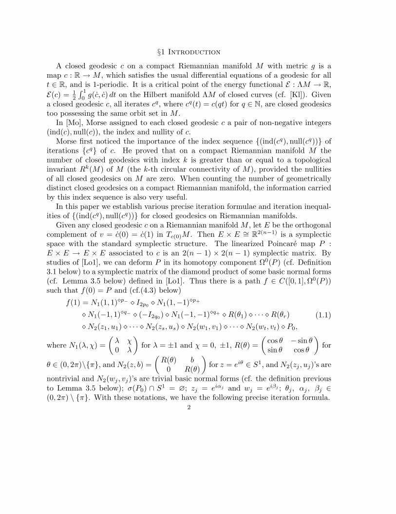
§1 Introduction

A closed geodesic c on a compact Riemannian manifold M with metric g is amap c : R → M , which satisfies the usual differential equations of a geodesic for allt ∈ R, and is 1-periodic. It is a critical point of the energy functional E : ΛM → R,E(c) = 1

2

∫ 1

0g(c, c) dt on the Hilbert manifold ΛM of closed curves (cf. [Kl]). Given

a closed geodesic c, all iterates cq, where cq(t) = c(qt) for q ∈ N, are closed geodesicstoo possessing the same orbit set in M .

In [Mo], Morse assigned to each closed geodesic c a pair of non-negative integers(ind(c), null(c)), the index and nullity of c.

Morse first noticed the importance of the index sequence (ind(cq), null(cq)) ofiterations cq of c. He proved that on a compact Riemannian manifold M thenumber of closed geodesics with index k is greater than or equal to a topologicalinvariant Rk(M) of M (the k-th circular connectivity of M), provided the nullitiesof all closed geodesics on M are zero. When counting the number of geometricallydistinct closed geodesics on a compact Riemannian manifold, the information carriedby this index sequence is also very useful.

In this paper we establish various precise iteration formulae and iteration inequal-ities of (ind(cq),null(cq)) for closed geodesics on Riemannian manifolds.

Given any closed geodesic c on a Riemannian manifold M , let E be the orthogonalcomplement of v = c(0) = c(1) in Tc(0)M . Then E × E ∼= R2(n−1) is a symplecticspace with the standard symplectic structure. The linearized Poincare map P :E × E → E × E associated to c is an 2(n − 1) × 2(n − 1) symplectic matrix. Bystudies of [Lo1], we can deform P in its homotopy component Ω0(P ) (cf. Definition3.1 below) to a symplectic matrix of the diamond product of some basic normal forms(cf. Lemma 3.5 below) defined in [Lo1]. Thus there is a path f ∈ C([0, 1], Ω0(P ))such that f(0) = P and (cf.(4.3) below)

f(1) = N1(1, 1)¦p− ¦ I2p0 ¦N1(1,−1)¦p+

¦N1(−1, 1)¦q− ¦ (−I2q0) ¦N1(−1,−1)¦q+ ¦R(θ1) ¦ · · · ¦R(θr)

¦N2(z1, u1) ¦ · · · ¦N2(zs, us) ¦N2(w1, v1) ¦ · · · ¦N2(wt, vt) ¦ P0,

(1.1)

where N1(λ, χ) =(

λ χ0 λ

)for λ = ±1 and χ = 0, ±1, R(θ) =

(cos θ − sin θsin θ cos θ

)for

θ ∈ (0, 2π)\π, and N2(z, b) =(

R(θ) b0 R(θ)

)for z = eiθ ∈ S1, and N2(zj , uj)’s are

nontrivial and N2(wj , vj)’s are trivial basic normal forms (cf. the definition previousto Lemma 3.5 below); σ(P0) ∩ S1 = ∅; zj = eiαj and wj = eiβj ; θj , αj , βj ∈(0, 2π) \ π. With these notations, we have the following precise iteration formula.

2

Theorem 1.1. For any closed geodesic c on an n-dimensional Riemannian manifoldM , there always holds

ind(cq) =q(ind(c) + p− + p0 − r) + 2r∑

j=1

E(qθj

2π)

− r − p− − p0 − 1 + (−1)q

2(q0 + q+)

+ 2(s∑

j=1

ϕ(qαj

2π)− s),

(1.2)

null(cq) =null(c) +1 + (−1)q

2(q− + 2q0 + q+)+

+ 2(r −

r∑

j=1

ϕ(qθj

2π) + s−

s∑

j=1

ϕ(qαj

2π) + t−

t∑

j=1

ϕ(qβj

2π)),

(1.3)

where E(a) = mink ∈ Z| k ≥ a, [a] = maxk ∈ Z| k ≤ a and ϕ(a) = E(a)− [a] .

In many applications, studies are reduced to iteration inequalities. The followingresults are proved in Section 4 of this paper.

Theorem 1.2. For any closed geodesic c on an n-dimensional Riemannian manifoldM , there always holds

qi(c)− n + 1 ≤ ind(cq) ≤ qi(c) + n− 1− null(cq), (1.4)

where i(c) = limq→∞ind(cq)

q is the mean index of the closed geodesic c.

Theorem 1.3. For any closed geodesic c on an n-dimensional Riemannian manifoldM , there always holds

q(ind(c) + null(c)− n + 1) + n− 1− null(c) ≤ ind(cq)

≤ q(ind(c) + n− 1)− n + 1− (null(cq)− null(c)).(1.5)

Inequalities (1.4) and (1.5) are partial results of Theorem 4.4 and 4.5 in Section4 of this paper. There we also consider the necessary and sufficient conditions underwhich the left or right equalities of (1.4) or (1.5) holds for some q. Further results oniterated indices can be found in Sections 3 and 4.

3

Our these results are used in Section 5 to study the stability and multiplicity ofthe closed geodesics on compact Riemannian manifolds including a new observationon two theorems of Hingston in [Hi1] and [Hi2].

Note that results proved in this paper including above theorems remain valid forclosed geodesics on Finsler manifolds.Remark 1.4. Comparing with normal forms of symplectic matrices obtained in[BTZ] and those used in [Lo1], the significant difference is that in [Lo1] the normalforms is further studied in the homotopy component Ω0(P ) of P ∈ Sp(2n− 2) whichallows one to greatly simplify the decomposition of symplectic matrix P and reduceall the iteration formulae to only 10 different simple patterns. This then yields theiteration formula Theorem 1.1 in terms of the decomposition of the end matrix P inΩ0(P ) and the iteration time q. In such a way, precise values of splitting numbersare also computed out explicitly.

§2 Prelimimaries

We first recall some notations and definitions in [BTZ]. Let M be an n-dimensionalcomplete connected C∞ Riemannian manifold. If c : [0, 1] → M is a closed geodesicwith c(0) = c(1) = p, and E is the orthogonal complement of v = c(0) = c(1) inTpM , then the linearized Poincare map of c defined by P : E ⊕ E → E ⊕ E withP : (X, Y ) 7→ (U(1),∇U(1)), where U is the unique Jacobi field along c determinedby U(0) = X and ∇U(0) = Y . The map P preserves the symplectic structure ω onE ⊕ E defined by

ω((X1, Y1), (X2, Y2)) = 〈X1, Y2〉 − 〈Y1, X2〉,

where 〈·, ·〉 is the usual inner product in E ∼= Rn−1.Note that we can choose an orthonormal basis such that E ∼= Rn−1 and E ⊕E ∼=

R2(n−1). With this equivalence, the linearized Poincare map P corresponds to asymplectic matrix which is still denoted by P , and the above symplectic structurecan be given on R2(n−1) by

ω(X, Y ) = −〈XJ, Y 〉

for X = (x1, · · · , x2n−2) ∈ R2n−2 and similar Y , where J =(

0 −In−1

In−1 0

).

Let Λ = Λ(M) be the space of piecewise C∞ curves c : I = [0, 1] → M suchthat c(0) = c(1), which is equipped with the compact-open topology induced by thedistance ρ(c, c′) = maxt∈I d(c(t), c′(t)). The energy functional E : Λ → R is defined

4

by E(c) = 12

∫ 1

0〈c, c〉dt. The critical points of E are the closed geodesics and the point

curves. For any closed geodesic c ∈ Λ, let VΛ(c) be the space of piecewise C∞ vectorfields X along c such that 〈X, c(t)〉 = 0 for all t and such that X(0) = X(1). Theindex form H : VΛ(c)× VΛ(c) → R of c is given by

H(X,Y ) =∫ 1

0

(〈∇X,∇Y 〉 − 〈R(X, c)c, Y 〉) dt,

where 〈·, ·〉 is the inner product induced by the Riemannian metric of the manifoldM . Note that we have abused the symbol 〈·, ·〉 in two different senses. We hope thatit will not cause any confusion. The index ind(c) of c as a closed geodesic is definedto be the index of H. The nullity null(c) of c is defined to be dimC kerC(H|VΛ(c)).Similarly the index indΩ(c) of a geodesic segment c : [0, 1] → M is defined to bethe index of the form H on the space VΩ(c) of piecewise C∞ vector fields X alongc such that 〈X, c(t)〉 = 0 for all t and such that X(0) = X(1) = 0. The nullityof c is defined by nullΩ(c) = dimC kerC(H|VΩ(c)). It is well known that there holdnull(c) = dimC kerC(P − id) and ind(c) ≥ indΩ(c). For t > 0, let µ(t) be the numberof linearly independent Jacobi fields Y along c with Y (0) = Y (t) = 0. Then theMorse index theorem for geodesic segments states that

indΩ(c) =∑

0<t<1

µ(t), nullΩ(c) = µ(1).

The concavity of the closed geodesic is defined by C(c) = ind(c) − indΩ(c). Thereholds 0 ≤ C(c) ≤ n− 1.

Let c : R → M be a geodesic such that c0 = c|[0,1] is a closed geodesic. Choosepoints 0 = t0 < t1 < · · · < tk = 1 such that there are no pairs of conjugate pointson c|[ti, ti+1]. Denote by J the vector space of continuous vector fields X along csuch that X|[ti + k, ti+1 + k] is a Jacobi field orthogonal to c for all i and all k ∈ Z.Denote the complexification of J by JC . For q ∈ N and z ∈ S1 = u ∈ C| |u| = 1,set

Jz = X ∈ JC |X(t + 1) = zX(t) ∀t ∈ R.Jz is a finite dimensional subspace of JC . A symmetric form Hz is defined on Jz by:

Hz(X,Y ) =∫ 1

0

(〈∇X,∇Y 〉 − 〈R(X, c)c, Y 〉) dt,

where we have extend 〈·, ·〉 to a Hermitian form and R to a complex linear tensor ofTM ⊗ C. We define

I(z) = indHz, N(z) = dimC kerCHz,5

and I0(z) = I(z) + N(z). Note that I(1) = ind(c0), N(1) = null(c0) and I0(1) =ind0(c0) = ind(c0) + null(c0). Denote the complexification of E by EC

∼= Cn−1 andextend the linear Poincare map P to a complex linear automorphism of EC ⊕EC

∼=Cn−1 ⊕ Cn−1.

We define the q fold iteration of the closed geodesic c0 by cq0(t) = c0(qt) for all

t ∈ R. The following well known result is due to Bott [Bo1] (cf. also [BTZ]).

Theorem 2.1. For z ∈ S1, (i) ind(cq0) =

∑zq=1 I(z), null(cq

0) =∑

zq=1 N(z).(ii) N(z) = dimC kerC(P − z id).(iii) I is locally constant near the points at which N(z) = 0 and the splitting

numbers of c0 at z are defined by

S±(z) = limθ→±0

I(zeiθ)− I(z) (2.1)

which satisfy 0 ≤ S±(z) ≤ N(z).(iv) I(z) = I(z), N(z) = N(z).

In this section, the Poincare map P : EC ⊕ EC → EC ⊕ EC can be viewed as a2(n− 1)× 2(n− 1) matrix when EC ⊕EC

∼= Cn−1 ⊕ Cn−1 is used. Here the matrixP acts from right to row vectors.

We define a Hermitian form ωh on EC ⊕ EC∼= Cn−1 ⊕ Cn−1 by

ωh((X1, Y1), (X2, Y2)) = i(〈X1, Y2〉 − 〈Y1, X2〉) = −i〈(X1, Y1)J, (X2, Y2)〉,

where i =√−1. On the subspace W ⊂ Cn−1 ⊕ Cn−1 with

W = (P − z id)−1(0, EC) = X ∈ Cn−1 ⊕ Cn−1|X(P − z id) ∈ (0,Cn−1), (2.2)

we defineHP,z(X, Y ) = iωh(XPz − id), Y ) = 〈X(P z − id)J, Y 〉.

SetCP (z) = indHP,z + dimC kerC HP,z − dimC kerC(P − z id). (2.3)

The following result was proved in [BTZ](Theorem 2.7)

Proposition 2.2. (i) I(z) = indΩ(c0) + CP (z).(ii) CP (z) depends only on P and z. The splitting numbers S±P (z) defined by (2.1)

satisfy:S±P (z) = lim

θ→±0CP (zeiθ)− CP (z), (2.4)

6

and are depend only on P and z.(iii) There holds 0 ≤ CP (z) ≤ n− 1.

The space V = EC ⊕EC∼= Cn−1 ⊕Cn−1 is a symplectic space with the standard

symplectic form ω. L = (0, EC) ∼= (0,Cn−1) is a Lagrangian subspace of V . Takinganother Lagrangian subspace L′ of V with

L ∩ L′ = 0, PL ∩ L′ = 0, (2.5)

for z ∈ S1, the following form on V is introduced in [BTZ],

Bz(X, Y ) = Bz(P, L, L′)(X,Y ) = iωh((P z−id)X,Y )+iωh((P z−id)X,π(P z−id)Y ),

where π is the projection of V onto L such that kerπ = L′. The following result wasproved in [BTZ] (Lemma 2.10 and the proof of (2.12) there).

Proposition 2.3. (i) kerBz = ker(P − z id).(ii) S±P (z) = limθ→±0 indBzeiθ − indBz.(iii) indBz(P, L, L′) − indBz(P, L, L′1) is independent of z if (L,L′) and (L,L′1)

satisfy (2.5).

§3 Further studies on splitting numbers of closed geodesics

In this section, we consider the relations of the splitting numbers of the closedgeodesics with the Krein type of the Poincare map or matrix P . As a matrix, P ∈L(R2(n−1)) is a symplectic matrix, i.e., P ∈ Sp(n − 1) = A ∈ L(R2(n−1))|AT JA =J, where AT is the transpose of A.

Definition 3.1. ([Lo1]) For any M ∈ Sp(n−1) the homotopy set of M in Sp(n−1)is defined by

Ω(M) = N ∈Sp(n− 1)|σ(N) ∩ S1 = σ(M) ∩ S1, and

dimC kerC(N − z id) = dimC kerC(M − z id), ∀z ∈ σ(M) ∩ S1.

Denote by Ω0(M) the path connected component of Ω(M) which contains M , andcall it the homotopy component of M in Sp(n− 1).

We now prove the following result.7

Theorem 3.2. For any M ∈ Ω0(P ) and z ∈ S1, there holds

S±P (z) = S±M (z). (3.1)

Thus the splitting numbers depend only on the homotopy component of the matrix Pand z ∈ S1.

Remark 3.3. The conjugacy class of P in Sp(n− 1) is defined by

[P ] = M−1PM |M ∈ Sp(n− 1).

It is clear that [P ] ⊂ Ω0(P ). So Theorem 2.11 of [BTZ] is a special case of ourTheorem 3.2.

Proof of the Theorem 3.2. Taking a C∞ path f : [0, 1] → Ω(P ) such that f(0) =P, f(1) = M , for any z ∈ S1 and t ∈ [0, 1] there holds

dimC kerC(P − z id) = dimC kerC(f(t)− z id) = dimC kerC(M − z id). (3.3)

Taking L = (0, EC) which is a Lagrangian subspace of V = EC ⊕ EC , for anyt0 ∈ [0, 1], by the continuity of f , there exist ε = ε(t0) and Lt0 such that

L ∩ Lt0 = 0, f(t)L ∩ Lt0 = 0, ∀t ∈ (t0 − ε, t0 + ε).

By the compactness of the set [0, 1], there exist k − 1 numbers 0 = t0 < t1 < · · · <tk = 1 and k Lagrangian subspaces L′i, i = 1, 2, · · · , k such that

L ∩ L′i = 0, f(t)L ∩ L′i = 0, ∀t ∈ [ti−1, ti], i = 1, · · · , k. (3.2)

Thus similarly to (2.5), by (3.2) we can define the form Bz(f(t), L, L′i) for t ∈[ti−1, ti], i = 1, · · · , k. By Proposition 2.3(i), there holds

dimC kerCBz(f(t), L, L′i) = dimC kerC(f(t)− z id) = dimC kerC(P − z id),

which does not depend on t ∈ [ti−1, ti]. Thus the index indBz(f(t), L, L′i) must beconstant for t ∈ [ti−1, ti], and there holds

indBz(f(ii−1), L, L′i) = indBz(f(ti), L, L′i).

By Proposition 2.3 (iii), we have that

indBz(f(ti), L, L′i)− indBz(f(ti), L, L′i+1)8

is constant in the variable z ∈ S1. Thus for each i = 0, 1, · · · , k − 1, the function

indBz(f(ti), L, L′i)− indBz(f(ti+1), L, L′i+1)

is constant. This implies that

indBz(P,L, L′0)− indBz(M, L,L′k)

does not depend on z ∈ S1. By Proposition 2.3(ii), there holds

S±P (z) = limθ→±0

indBzeiθ(P, L, L′0)− indBz(P, L, L′0)

= limθ→±0

indBzeiθ(M,L, L′k)− indBz(M,L, L′k)

= S±M (z).

¤We now recall the diamond product of two matrices. For two even order matrices

of square block form

M1 =(

A1 B1

C1 D1

)

2i×2i

and M2 =(

A2 B2

C2 D2

)

2j×2j

,

the ¦-product of M1 and M2 is defined to be the 2(i + j)× 2(i + j) matrix M1 ¦M2:

M1 ¦M2 =

A1 0 B1 00 A2 0 B2

C1 0 D1 00 C2 0 D2

,

and M¦k1 to be the k-times ¦-product of M1. Note that the ¦-product is associative

and the ¦-product of two symplectic matrices is still symplectic. For two vectorsX = (x1, y1) ∈ Ci⊕Ci and Y = (x2, y2) ∈ Cj⊕Cj , we define X¦Y = (x1, x2, y1, y2) ∈Ci+j ⊕ Ci+j .

Theorem 3.4. For P ∈ Sp(n− 1) and Pk ∈ Sp(nk), k = 1, 2 with n1 + n2 = n− 1such that P = P1 ¦ P2, there holds

S±P (z) = S±P1(z) + S±P2

(z), ∀z ∈ S1. (3.4)9

Proof. Let E = EC ⊕ EC∼= Cn−1 ⊕ Cn−1 and Ek = Cnk−1, k = 1, 2. For X =

(x1, y1) ∈ E1 ⊕ E1 and Y = (x2, y2) ∈ E2 ⊕ E2, it is clear that (X ¦ Y )(P1 ¦ P2) =(XP1) ¦ (Y P2) and

P1 ¦ P2 − z id = (P1 − z id) ¦ (P2 − z id).

By definition (2.2), we have

(P − z id)−1(0, Ec) = (P1 − z id)−1(0, E1) ¦ (P2 − z id)−1(0, E2).

Let

Jk =(

0 −Ink

Ink0

), k = 1, 2.

Then there holds J = J1 ¦J2. For any X, Y ∈ (P −z id)−1(0, EC) with X = X1 ¦X2

and Y = Y1 ¦ Y2, Xk, Yk ∈ (Pk − z id)−1(0, Ek), k = 1, 2, by definition, there holds

HP,z(X,Y ) = 〈X(P z − id)J, Y 〉= 〈(X1 ¦X2)((P1z − id)J1 ¦ (P2z − id)J2), Y1 ¦ Y2〉= 〈(X1(P1z − id)J1) ¦ (X2(P2z − id)J2), Y1 ¦ Y2〉= 〈X1(P1z − id)J1, Y1〉+ 〈X2(P2z − id)J2, Y2〉= HP1,z(X1, Y1) + HP2,z(X2, Y2).

It is clear that

dimC kerC(P1 ¦ P2 − z id) = dimC kerC(P1 − z id) + dimC kerC(P2 − z id).

By definition, there holds

CP (z) = (ind + dimC kerC)HP,z − dimC kerC(P − z id)

= (ind + dimC kerC)HP1,z − dimC kerC(P1 − z id)

+ (ind + dimC kerC)HP2,z − dimC kerC(P2 − z id)

= CP1(z) + CP2(z).

By Proposition 2.2, there holds

S±P (z) = limθ→±0

CP (zeiθ)− CP (z)

= limθ→±0

CP1(zeiθ)− CP1(z) + limθ→±0

CP2(zeiθ)− CP2(z)

= S±P1(z) + S±P2

(z).10

¤Recall the concept of the basic normal forms of symplectic matrices defined in

[Lo1]. They are the following symplectic matrices:

N1(λ, χ), R(θ), N2(θ, b)

with N1(λ, χ) =(

λ χ0 λ

)for λ = ±1 and χ = 0,±1, R(θ) =

(cos θ, − sin θsin θ cos θ

)for

θ ∈ (0, 2π) \ π, and

N2(z, b) =(

R(θ) b0 R(θ)

)

for z = eiθ ∈ S1, θ ∈ (0, 2π) \ π and b =(

b1 b2

b3 b4

), bi ∈ R, b2 6= b3. It is clear

that the matrix N2(z, b) is symplectic if and only if

(b2 − b3) cos θ + (b1 + b4) sin θ = 0. (3.5)

In [Lo1], the basic normal forms N1(1,−1), N1(−1, 1), N2(z, b) and N2(z, b) withz = eiθ ∈ S1 \ ±1 satisfying (b2 − b3) sin θ > 0 are called trivial, and all the otherbasic normal forms are called nontrivial. The following result was proved in [Lo1].

Lemma 3.5. For any P ∈ Sp(n−1), there is a path f ∈ C∞([0, 1], Ω0(P )) such thatf(0) = P and

f(1) = P1 ¦ · · · ¦ Pk ¦ P0

where the integer k ∈ [0, n− 1], each Pi is a basic normal form of eigenvalues on S1

for i = 1, · · · , k, and the symplectic matrix P0 satisfies σ(P0) ∩ S1 = ∅.

For the splitting numbers of the basic normal forms, we have the following result.

Proposition 3.6. (i) For any P ∈ Sp(n− 1) and z ∈ S1, there holds

S±P (z) = S∓P (z). (3.6)

(ii) If P = N1(1, χ) =(

1 χ0 1

)with χ = 0, 1, there holds S±P (1) = 1.

(iii) If P = N1(1,−1) =(

1 −10 1

), there holds S±P (1) = 0.

(iv) If P = N1(−1, χ) =(−1 χ

0 −1

)with χ = 0, −1, there holds S±P (−1) = 1.

11

(v) If P = N1(−1, 1) =(−1 1

0 −1

), there holds S±P (−1) = 0.

(vi) If P = R(θ) with θ ∈ (0, 2π) \ π, there holds S+P (eiθ) = 0, S−P (eiθ) = 1.

(vii) If P = N2(z, b) with z = eiθ, θ ∈ (0, 2π) \ π, there holds

S±P (eiθ) = 1, if P is non-trivial, i.e., (b2 − b3) sin θ < 0,

S±P (eiθ) = 0, if P is trivial, i.e., (b2 − b3) sin θ > 0.

Proof. Step 1. Proof of (i). It is clear from I(z) = I(z) and the properties of theeigenvalues of the symplectic matrices.

Step 2. Proof of (vii). Let P = N2(ω, b) =(

R(θ) b0 R(θ)

), θ ∈ (0, 2π) \ π,

ω = eiθ. Note that P is symplectic if and only if

(b2 − b3) cos θ + (b1 + b4) sin θ = 0. (3.7)

In this case, n = 3 and EC = C2.For z = eiϕ, ϕ 6= θ but ϕ close to θ, the matrix R(θ) − z id is invertible. If

(x1, x2, y1, y2)(P − z id) = (0, 0, ∗, ∗) ∈ (0,C2), there holds x1 = x2 = 0. This impliesthat (P−z id)−1(0, EC) = (0, EC). For any X = (0, 0, y1, y2) and Y = (0, 0, u1, u2) ∈(P − z id)−1(0, EC), there holds

HP,z(X,Y ) = 〈X(P z − id)J, Y 〉= z〈(0, 0, ∗, ∗)J, (0, 0, u1, u2)〉 = z〈(∗, ∗, 0, 0), (0, 0, u1, u2)〉 = 0,

Here and below ∗ denotes all complex numbers we do not care what they are. Thus(ind + dimC kerC)HP,z = 2 and dimC kerC(P − z id) = 0. It implies CP (z) = 2.

For z = eiϕ, ϕ = θ, there holds

(P − z id)−1(0, EC) = (x1, ix1, y1, y2)|x1, y1, y2 ∈ C.

In fact, (x1, x2, y1, y2)(P − z id) = (0, 0, ∗, ∗) ∈ (0,C2), if and only if (x1, x2)(R(θ)−z id) = 0, which implies x2 = ix1.

For X = (x1, ix1, y1, y2) and Y = (x2, ix2, u1, u2), by direct computation, thereholds

HP,z(X,Y ) = 〈X(P z − id)J, Y 〉 = z(x1x2b1 + ix1x2b3 − ix1x2b2 + x1x2b4)

= x1x2z(b1 + b4 − i(b2 − b3)).12

¿From (3.7), there holds

HP,z(X, Y ) = x1x2z(− (b2 − b3) cos θ

sin θ− i(b2 − b3)

)

= −x1x2(b2 − b3)(cos θ

sin θ(cos θ − i sin θ) + i cos θ + sin θ

)

= − x1x2

sin2 θ(b2 − b3) sin θ

and

HP,z(X, X) = − |x1|2sin2 θ

(b2 − b3) sin θ..

If (b2−b3) sin θ 6= 0, there holds dimC kerC HP,z = 2 and dimC kerC(P−z id) = 1. If(b2− b3) sin θ < 0, there holds indHP,z = 0. This implies CP (eiθ) = 1. By definition,there holds S±P (eiθ) = 2− 1 = 1. If (b2− b3) sin θ > 0, there holds indHP,z = 1. ThusCP (eiθ) = 2. By definition, there holds S±P (eiθ) = 2− 2 = 0.

Since the proofs for (ii)-(vi) are similar to that in Step 2, we are sketchy in therest of the proofs.

Step 3. Proof of (ii). If P = N1(1, 0), In this case n = 2. It is easy to see that

(P − z id)−1(0, EC) = EC ⊕ EC , if z = 1

(P − z id)−1(0, EC) = 0 ⊕ EC , if z 6= 1.

By a direct computation, there holds

(ind + dimC kerC)HP,z = 2, if z = 1

(ind + dimC kerC)HP,z = 1, if z 6= 1.

Thus by definition, there holds CP (z) = 1 where z 6= 1, and CP (1) = 0. ThenS±P (1) = 1 follows from Proposition 2.2.

In the case of P = N1(1, 1), the proof is similar to the above case, and is thusomitted. The proofs of (iii)-(v) are similar to that of (ii), and are also omitted too.

Step 4. Proof of (vi). Suppose P = R(θ), 0 < θ < π, and z = eiϕ = cos ϕ+i sin ϕ.Then by a direct computation we have

W = (P − z id)−1(0, EC) = (x,−cos θ − z

sin θx) ∈ C⊕ C| x ∈ C.

13

For X = (x,− cos θ−zsin θ x) and Y = (y,− cos θ−z

sin θ y), there holds

HP,z(X, Y ) = xy2(cos θ − cos ϕ)

sin θ.

¿From this we get

dimC kerC(P − z id) =

0, if 0 < ϕ < θ < π,

0, if 0 < θ < ϕ < π,

1, if 0 < θ = ϕ < π,

and

(ind + dimC kerC)HP,z =

1, if 0 < ϕ < θ < π,

0, if 0 < θ < ϕ < π,

1, if 0 < θ = ϕ < π.

Thus by definition, there holds

CP (eiϕ) =

1, 0 < ϕ < θ < π,

0, 0 < θ < ϕ < π,

0, 0 < θ = ϕ < π.

Therefore we have S+P (eiθ) = 0 and S−P (eiθ) = 1 by Proposition 2.2. The proof for

P = R(θ), π < θ < 2π, is similar, and thus is omitted. ¤Denote the complex root vector space of matrix P belonging to eigenvalue λ by

Eλ(P ) = ∪k≥1 kerC(P − λid)k). On Cn−1 ⊕ Cn−1, the Krein form is defined byωh(x, y) = −√−1〈xJ, y〉 for x, y ∈ Cn−1 ⊕ Cn−1 (cf. [YS]). It is well known that ifλ ∈ S1, the restriction ωh|Eλ(P ) of ωh to Eλ(P ) is non-degenerate. Denote the totalmultiplicities of positive and negative eigenvalues of ωh|Eλ(P ) by p and q respectively.The integer pair (p, q) is called the Krein type of λ. In [Lo1] the ultimate typeof λ ∈ S1 for P was introduced. More precisely for any basic normal form M andλ ∈ S1 ∩ σ(M), the ultimate type (p, q) of λ for M is defined to be its usual Kreintype if M is nontrivial, and to be (0, 0) if M is trivial. When σ(P ) ∩ S1 = ∅, theultimate type of any z ∈ S1 for P is defined by (0, 0). For any symplectic matrix P ,by Lemma 3.5, denoting the ultimate type of λ for Pi by (pi, qi) for 1 ≤ i ≤ k, lettingp =

∑ki=0 pi and q =

∑ki=0 qi, the integer pair (p,q) is defined to be the ultimate type

of λ for P . This definition is well defined and the ultimate type is constant on Ω0(P )for fixed λ ∈ S1. For symplectic matrix P and its eigenvalue λ ∈ S1, the Krein type(s, t) and ultimate type (p, q) satisfy (cf. [Lo1])

s− p = t− q. (3.8)

14

Theorem 3.7. For any z ∈ S1 and symplectic matrix P , there holds

S+P (z) = p(z), S−P (z) = q(z), (3.9)

where (p(z), q(z)) is the ultimate type of z for P .

Proof. For the trivial basic normal forms, (3.9) is proved in the Proposition 3.6. Forthe nontrivial basic normal forms, it leaves to verify the Krein type of these normalforms coincides with the values obtained in Proposition 3.6. These have already beencomputed in Theorem 4.11 of [Lo1]. The general case follows from Theorem 3.4. ¤Proposition 3.8. For any z ∈ S1 and symplectic matrix P , there holds

S+P (z)− S−P (z) = sP (z)− tP (z), (3.10)

and there holds

0 ≤ N(z)− S−P (z) ≤ sP (z), 0 ≤ N(z)− S+P (z) ≤ tP (z), (3.11)

where (sP (z), tP (z)) is the Krein type of z for P , and N(z) = dimC kerC(P − z id)(cf. Theorem 2.1).

Proof. (3.10) follows from (3.8) and (3.9). By (3.9), (3.11) was proved in [LZ]. Infact, by Theorem 3.4 and Lemma 3.5, we only need to prove (3.11) for basic normalforms. This follows from a direct computation. ¤Remark 3.9. Note that by Theorem 3.7, the splitting numbers defined by theabove (2.1) coincide with the splitting numbers defined by (1.3) of [Lo1] via paths insymplectic group and ω-indices.

§4 Iterated index formulae of the closed geodesics

In this section, we study various iteration inequalities and the precise iterationformulae of the Morse index of closed geodesics. Let c : R → M be a geodesic suchthat c0 = c|[0, 1] is a closed geodesic. The mean index of c0 is defined by (cf. [Bo1]and [Rad]):

i(c0) = limq→∞

ind(cq0)

q=

12π

∫ 2π

0

I(eiθ) dθ ∈ R. (4.1)

The following result gives an estimate for the index pair (I(z), N(z)) defined insection 2.

15

Theorem 4.1. Let c0 be a closed geodesic on an n-dimensional Riemannian manifoldM . Denote its Poincare map by P .

(i) For z = eiω ∈ S1 \ 1, there always holds

ind(c0)) + null(c0)− n + 1 ≤ I(eiω) ≤ ind(c0) + n− 1−N(eiω). (4.2)

(ii) The left equality in (4.2) holds for some z = eiω ∈ S1\±1 if and only if thereholds I2p ¦N1(1,−1)¦q ¦K ∈ Ω0(P ) for some non-negative integers p and q satisfying0 ≤ p + q ≤ n − 1 and K ∈ Sp(n − 1 − p − q) satisfying K = R(θ1) ¦ · · · ¦ R(θk),0 < θi ≤ ω < π for 0 < ω < π or 0 < θi ≤ 2π − ω < π for π < ω < 2π.

The left equality in (4.2) holds for z = −1 if and only if there holds

I2p ¦N1(1,−1)¦q ¦ (−I2l) ¦N1(−1,−1)¦h ¦K ∈ Ω0(P )

with K = R(θ1) ¦ · · · ¦R(θr), p + q + l + h + r = n− 1, and 0 < θi < π.(iii) The left equality in (4.2) holds for all z = eiω ∈ S1 \ 1 if and only if

I2p ¦ N1(1,−1)¦(n−1−p) ∈ Ω0(P ) for some integer p ∈ [0, n − 1]. Specifically in thiscase, all the eigenvalues of P must be 1 and null(c0) = n− 1 + p ≥ n− 1.

(iv) The right equality in (4.2) holds for some z = eiω ∈ S1 \ ±1 if and onlyonly if there holds I2p ¦N1(1, 1)¦r ¦K ∈ Ω0(P ) for some non-negative integers p andr satisfying p + r ≤ n− 1 and K = R(2π− θ1) ¦ · · · ¦R(2π− θk), 0 < θi ≤ ω < π for0 < ω < π or 0 < θi ≤ 2π − ω < π for π < ω < 2π, p + r + k = n− 1.

If z = eiω = −1, there holds I2p ¦ N1(1, 1)¦r ¦ (−I2s) ¦ N1(−1, 1)¦t ¦K ∈ Ω0(P ),where K = R(2π−θ1)¦· · ·¦R(2π−θk), satisfying 0 < θi < π and p+r+s+t = n−1.

(v) The right equality in (4.2) holds for all z = eiω ∈ S1 \ 1 if and only ifI2p ¦ N1(1, 1)¦(n−1−p) ∈ Ω0(P ) for some integer p ∈ [0, n − 1]. Specifically in thiscase, all the eigenvalues of P must be 1, and there holds null(c0) = n−1+p ≥ n−1.

(vi) Both equalities in (4.2) hold for all z = eiω ∈ S1\1 if and only if P = I2n−2.

Proof. (i) By Lemma 3.5, there is a path f ∈ C([0, 1], Ω0(P )) such that f(0) = Pand

f(1) = N1(1, 1)¦p− ¦ I2p0 ¦N1(1,−1)¦p+

¦N1(−1, 1)¦q− ¦ (−I2q0) ¦N1(−1,−1)¦q+

¦R(θ1) ¦ · · · ¦R(θr)

¦N2(z1, u1) ¦ · · · ¦N2(zs, us)

¦N2(w1, v1) ¦ · · · ¦N2(wt, vt)¦ P0,

(4.3)

16

where N2(zj , uj)’s are nontrivial and N2(wj , vj)’s are trivial basic normal forms ofsymplectic matrices; σ(P0) ∩ S1 = ∅; zj = eiαj and wj = eiβj ; θj , αj , βj ∈(0, 2π) \ π. Since I(z) = I(z) and N(z) = N(z) (cf. Theorem 2.1), we can supposez = eiω, 0 < ω < π. By definition, there holds

I(z)− I(1) = S+P (1) +

∑

0<θ<ω

(S+P (eiθ)− S−P (eiθ))− S−P (eiω), (4.4)

where the summation on the right side of (4.4) has in fact only finite many non-zero terms. By Theorem 3.4 and Proposition 3.6, and S+

P (z) = S−P (z), there holdS+

P (1) = p0 + p−,∑

0<θ<ω(S+P (eiθ)− S−P (eiθ)) = −k + l, 0 ≤ k + l ≤ r, where k ≥ 0

is the number of θj ’s in (4.3) such that 0 < θj < ω and l ≥ 0 is the number of θj ’s in(4.3) such that 2π − ω < θj < 2π, q1 ≡ S−P (eiω) is the sum of the numbers of θj = ωand αj = ω or 2π − αj = ω. Noticing null(c0) = 2p0 + p− + p+, there holds

I(z)− I(1) = p0 + p− + l − k − q1 = null(c0) + l − p0 − p+ − k − q1. (4.5)

By p0 + p+ + k + q1 ≤ n− 1, there holds

I(z)− I(1) ≥ null(c0)− n + 1. (4.6)

By k ≥ 0, p0 + p− + l ≤ n− 1 and q1 ≤ N(z), there holds

I(z)− I(1) ≤ p0 + p− + l − q1 ≤ n− 1−N(z). (4.7)

The inequalities (4.2) then follow from I(1) = ind(c0).If z = −1, then ω = π and

∑

0<θ<ω

(S+P (eiθ)− S−P (eiθ)) = −r1 + r2, r1 + r2 = r, (4.8)

where r1 is the number of θj ’s in (4.3) such that 0 < θj < π, and r2 is the number ofθj ’s in (4.3) such that π < θj < 2π, S−P (−1) = q0 + q+. Thus we have

I(−1)− I(1) = p0 + p− − r1 + r2 − q0 − q+. (4.9)

Noticing that N(−1) = q− + 2q0 + q+ ≥ q0 + q+, we get the estimate (4.2).(ii) By (4.2) and (4.5), the left equality in (4.2) holds for z = eiω ∈ S1 \ ±1

if and only if l − p0 − p+ − k − q1 = −n + 1, so we must have l = 0 and q1 is17

the number of ω = θj ’s in (4.3), i.e., no term N2(zj , uj) can appear in (4.3), sinceN2(zj , uj) ∈ Sp(3− 1) and S−M (z1) = 1 < 3− 1 = 2, where M = N2(zj , uj).

By (4.2), (4.9), and null(c0) = 2p0 + p+ + p−, the left equality in (4.2) holds forz = −1 if and only if

p+ + p0 + r1 + q0 + q+ − r2 = n− 1.

It follows that r2 = 0 and p+ + p0 + r1 + q0 + q+ = n− 1. Thus we have proved 2o.(iv) Similarly by (4.2) and (4.5), the right equality in (4.2) holds for z = eiω ∈

S1 \ ±1 if and only if

p0 + p− + l + N(eiω)− k − q1 = n− 1. (4.10)

But it is clear that p0 + p−+ l +N(eiω) ≤ n− 1. So we have k = q1 = 0. Thus (4.10)implies that no term of N2(zj , uj) or N2(wj , vj) can appear in (4.3). Then N(eiω) isthe number of R(θj)’s in (4.3) such that θj = 2π − ω.

The right equality in (4.2) holds for z = −1 if and only if

p0 + p− + q0 + q− + r2 − r1 = n− 1.

It implies r1 = 0 and p0 + p− + q0 + q− + r2 = n− 1. Thus we have proved (iv).(iii), (v), and (vi) are the direct consequence of (ii) and (iv). ¤We note that (4.2) improves the estimates given in Lemma 3.1 of [BTZ], where

the following estimate was proved:

|I(eiω)− ind(c0)| ≤ n− 1.

The following Lemma should be compared with Lemma 3.2 in [BTZ].

Lemma 4.2. Let z = eiω, 0 < ω ≤ π.(i) If I(z)−I(1) ≥ m > 0, then I2p0 ¦N1(1, 1)¦p− ¦R(2π−θ1)¦ · · · ¦R(2π−θl)¦M

∈ Ω0(P ) for some symplectic matrix M with p0 + p− + l ≥ m and 0 < θj < ω.(ii) If I(z)+N(z)− I(1)−N(1) ≤ −m < 0, then I2p0 ¦N1(1,−1)¦p+ ¦R(θ1)¦ · · · ¦

R(θk) ¦M1 ∈ Ω0(P ) for some symplectic matrix M1 with 0 < θj < ω, j = 1, · · · , k,and p0 + p+ + k ≥ m.

Proof. We use notations in the proof of Theorem 4.1.(i) follows from (4.3) and (4.5), I(z)− I(1) = p0 + p− + l − k − q1 ≤ p0 + p− + l

and (4.9), I(−1)− I(1) = p0 + p− − r1 + r2 − q0 − q+ ≤ p0 + p− + r2.18

(ii) follows from I(z)+N(z)−I(1)−N(1) = −p0−p+−k+ l+N(z)−q1 ≥ −p0−p+−k, and I(−1)+N(−1)−I(1)−N(1) = −p+−p0−r1+r2+q−+q0 ≥ −p+−p0−r1,where we have used (iii) of Theorem 2.1. ¤

Using (4.1) and the fact

limq→∞

null(cq0)

q=

12π

∫ 2π

0

N(eiθ) dθ = 0,

the following result is direct a consequence of Theorem 4.1.

Corollary 4.3. For any closed geodesic c0 on an n-dimensional Riemannian mani-fold, there always holds

ind(c0)) + null(c0)− n + 1 ≤ i(c0) ≤ ind(c0) + n− 1. (4.11)

We notice that (4.11) improves a related result given in Theorem 1.4 of [Rad]. Asa consequence of the above result, we have the following estimate.

Theorem 4.4. (i) For any closed geodesic c0 on an n-dimensional Riemannianmanifold, there always holds

qi(c0)− n + 1 ≤ ind(cq0) ≤ qi(c0) + n− 1− null(cq

0), ∀q ∈ N. (4.12)

(ii) The right equality in (4.12) holds for some q ∈ N if and only if

I2p ¦N1(1,−1)¦(n−1−p) ∈ Ω0(P )

for some integer p ∈ [0, n− 1]. Specifically in this case, all the eigenvalues of P equalto 1 and null(c0) = n− 1 + p ≥ n− 1.

(iii) The left equality in (4.12) holds for some q ∈ N if and only if

I2p ¦N1(1, 1)¦(n−1−p) ∈ Ω0(P )

for some integer p ∈ [0, n− 1]. Specifically in this case, all the eigenvalues of P mustbe 1, and there holds null(c0) = n− 1 + p ≥ n− 1.

(iv) Both equalities in (4.12) hold for some q ∈ N if and only if P = I2n−2.

Proof. Replacing c0 by cq0 in (4.11), and noting that i(cq

0) = qi(c0), we obtain theinequalities (4.12). The right(left) equality in (4.12) holds if and only if the left(right)equality in (4.2) holds for almost all z ∈ S1. Thus (ii)-(iv) follow from Theorem 4.1.¤

19

Corollary 4.5. For any closed geodesic c0 on an n-dimensional Riemannian mani-fold, we have the following equivalent statements:

(i) i(c0) > 0 ⇔ ind(cq0) is unbounded ⇔ limq→+∞ ind(cq

0) = +∞.(ii) i(c0) = 0 ⇔ ind(cq

0) is bounded ⇔ ind(cq0) = 0, ∀q ∈ N.

Proof. From (4.12), we get the statement of (i).The statement i(c0) = 0 ⇔ ind(cq

0) is bounded follows from (4.12) directly.We now prove i(c0) = 0 ⇔ ind(cq

0) = 0, ∀q ∈ N. The “⇐” statement followsfrom the definition of i(c0). Conversely, supose i(c0) = 0. Since I(z) ≥ 0 is locallyconstant on S1 except on at most finitely many points z1, . . . , zk in S1. By (4.1) weget I(z) = 0 for all z ∈ S1 \ z1, . . . , zk. By the definition (2.1) of splitting numbersand (iii) of Theorem 2.1, we get 0 ≤ I(zj) ≤ I(z) for z ∈ S1 sufficiently close to zj

with 1 ≤ j ≤ k. This proves I(z) = 0 for all z ∈ S1. Thus by (i) of Theorem 2.1, wehave ind(cq

0) =∑

zq=1 I(z) = 0 for all q ∈ N. ¤

From (4.11), we note that ind(c0) + null(c0) > n − 1 is a sufficient condition fori(c0) > 0.

Theorem 4.6. (i) For any closed geodesic c0 on an n-dimensional Riemannianmanifold, there always holds

q(ind(c0) + null(c0)− n + 1) + n− 1− null(c0) ≤ ind(cq0)

≤ q(ind(c0) + n− 1)− n + 1− (null(cq0)− null(c0)).

(4.13)

(ii) The left equality in (4.13) holds for some q > 2 if and only if there holdsI2p0 ¦N1(1,−1)¦p+ ¦K ∈ Ω0(P ) for some non-negative integers p0 and p+ satisfying0 ≤ p0 + p+ ≤ n− 1 and K ∈ Sp(n− 1− p0− p+) satisfying K = R(θ1) ¦ · · · ¦R(θk),0 < θi ≤ ω < π for 0 < ω < 2π/q.

The left equality in (4.13) holds for q = 2 if and only if there holds

I2p0 ¦N1(1,−1)¦p+ ¦ (−I2q0) ¦N1(−1,−1)¦q+ ¦K ∈ Ω0(P )

with K = R(θ1) ¦ · · · ¦R(θr), p0 + p+ + q0 + q+ + r = n− 1, and 0 < θi < π.(iii) The right equality in (4.13) holds for some q > 2 if and only if there holds

I2p0 ¦ N1(1, 1)¦p− ¦K ∈ Ω0(P ) for some non-negative integers p0 and p− satisfyingp0 + p− ≤ n− 1 and K = R(2π − θ1) ¦ · · · ¦R(2π − θk), 0 < θi ≤ 2π/q.

If q = 2, there holds I2p0 ¦N1(1, 1)¦p− ¦ (−I2q0)¦N1(−1, 1)¦q− ¦K ∈ Ω0(P ), whereK = R(2π−θ1)¦· · ·¦R(2π−θk), satisfying 0 < θi < π and p0 +p−+q0 +q− = n−1.

20

(iv) Both equalities in (4.13) hold for some q ∈ N if and only if P = I2n−2.

Proof. By the Bott formula (Theorem 2.1), summing (4.2) up over all q-th roots ofunit except z = 1, we obtain (4.13). The equality conditions follow from (ii) and (iv)of Theorem 4.1. ¤

For example, on M = Sn with the standard metric, every prime closed geodesicc0 is a great circle and by direct computation we obtain ind(c0) = n − 1, ind(cq

0) =(2q − 1)(n− 1). So the right equality in (4.13) holds.

For symplectic paths in Sp(n) or the fundamental solution of a linear Hamiltoniansystem, estimates similar to the above ones in this section were proved in [LL1] and[LL2]. We note that the differential dφt(x) of the geodesic flows φt(x) are symplecticpaths in the tangent bundle of the Riemannian manifolds, but in general they are notpaths in Sp(n)-the symplectic matrix group in R2n. Moreover, the method we usedhere is different from those of [LL1] and [LL2]. Motivated by the precise iterationformulae in [Lo2] for symplectic paths in Sp(n), we have

Theorem 4.7. Let c0 be any closed geodesic on an n-dimensional Riemannian man-ifold. Denote its Poincare map by P . Let f ∈ C([0, 1],Ω0(P )) such that f(0) = Pand

f(1) = P1 ¦ · · · ¦ Pk ¦ P0 (4.14)

is given by the representation (4.3), where each Pj is a basic normal form symplecticmatrix for 1 ≤ j ≤ k and σ(P0) ∩ S1 = ∅. Then the iteration formulae (1.2) and(1.3) hold.

Proof. By Proposition 3.6 and Remark 3.9, (1.2) and (1.3) follow directly from The-orem 1.3 of [Lo2]. Here we give a somewhat different proof for (1.2).

By Bott formula Theorem 2.1, there holds ind(cq0) =

∑zq=1 I(z). The index I(z)

for z ∈ S1 is determined by I(1) and the splitting numbers of the matrix P via (4.4).By (4.14), we choose k nonnegative integers Ij(1)| j = 0, 1, · · · , k such that

I(1) = I1(1) + · · ·+ Ik(1) + I0(1). (4.15)

For any z ∈ S1, we extend the definition of Ij to z by

Ij(z) = Ij(1) + S+Pj

(1) +∑

0<θ<ω

(S+Pj

(eiθ)− S−Pj(eiθ))− S−Pj

(eiω), (4.16)

where Pj is a basic normal form given by (4.3) and (4.14). Thus by (4.4), (4.15) andthe property

S±P (eiθ) =k∑

j=0

S±Pj(eiθ),

21

from (4.16) we obtain

I(z) =k∑

j=0

Ij(z). (4.17)

Then

ind(cq0) =

∑zq=1

I(z) =k∑

j=0

∑zq=1

Ij(z) =k∑

j=0

IqPj

, (4.18)

where IqPj≡ ∑

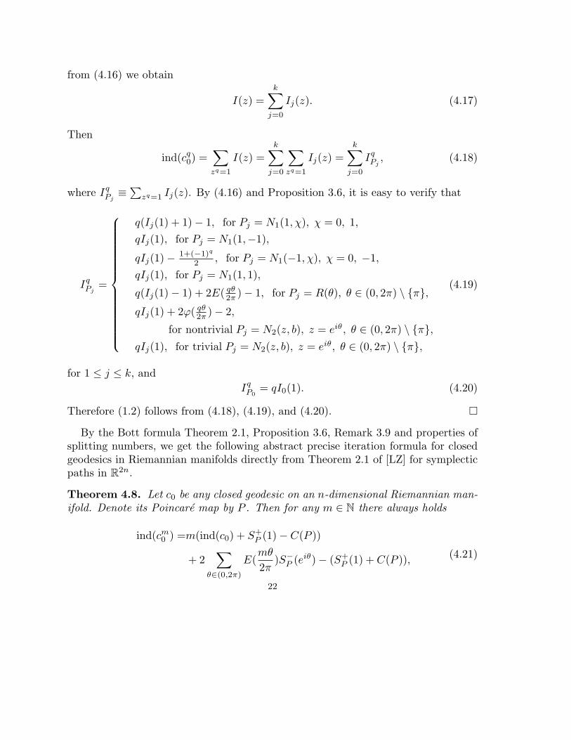
zq=1 Ij(z). By (4.16) and Proposition 3.6, it is easy to verify that

IqPj

=

q(Ij(1) + 1)− 1, for Pj = N1(1, χ), χ = 0, 1,

qIj(1), for Pj = N1(1,−1),

qIj(1)− 1+(−1)q

2 , for Pj = N1(−1, χ), χ = 0, −1,

qIj(1), for Pj = N1(1, 1),

q(Ij(1)− 1) + 2E( qθ2π )− 1, for Pj = R(θ), θ ∈ (0, 2π) \ π,

qIj(1) + 2ϕ( qθ2π )− 2,

for nontrivial Pj = N2(z, b), z = eiθ, θ ∈ (0, 2π) \ π,qIj(1), for trivial Pj = N2(z, b), z = eiθ, θ ∈ (0, 2π) \ π,

(4.19)

for 1 ≤ j ≤ k, andIqP0

= qI0(1). (4.20)

Therefore (1.2) follows from (4.18), (4.19), and (4.20). ¤

By the Bott formula Theorem 2.1, Proposition 3.6, Remark 3.9 and properties ofsplitting numbers, we get the following abstract precise iteration formula for closedgeodesics in Riemannian manifolds directly from Theorem 2.1 of [LZ] for symplecticpaths in R2n.

Theorem 4.8. Let c0 be any closed geodesic on an n-dimensional Riemannian man-ifold. Denote its Poincare map by P . Then for any m ∈ N there always holds

ind(cm0 ) =m(ind(c0) + S+

P (1)− C(P ))

+ 2∑

θ∈(0,2π)

E(mθ

2π)S−P (eiθ)− (S+

P (1) + C(P )), (4.21)

22

where C(P ) is defined byC(P ) =

∑

0<θ<2π

S−P (eiθ).

Note that the Poincare map P of a closed geodesic c0 on an n-dimensional Rie-mannian manifold M corresponds to a symplectic matrix. For any matrix P ∈Sp(n − 1), the elliptic height e(P ) of P is defined by the total algebraic mul-tiplicity of all eigenvalues of P on the unit circle S1. We note that there holds0 ≤ e(P ) ≤ 2(n − 1). P is elliptic if e(P ) = 2(n − 1), and it is hyperbolic ife(P ) = 0. The closed geodesic c0 is elliptic (hyperbolic) if its Poincare map iselliptic (hyperbolic). The elliptic height e(c0) of a closed geodesic c0 is defined bye(c0) = e(P ), where P is the Poincare map of c0.

Parallel to Theorems 2.2 and 2.4 of [LZ], we have the following results in Morseindices whose proofs follow directly from those in [LZ],Theorem 4.11 of [LZ], theabove Theorem 3.7, and the Remark 3.9.

Theorem 4.9. For any closed geodesic c0 with its Poincare map P , and any m ∈ N,there always holds

null(cm0 )− e(P )

2≤ ind(cm+1

0 )− ind(cm0 )− ind(c0)

≤ null(c0)− null(cm+10 ) +

e(P )2

.

(4.22)

Thus we have

ind(cm0 ) + ind(c0)− ind(cm+1

0 ) + null(cm0 ) ≤ n− 1 (4.23)

and

ind(cm+10 )− ind(cm

0 )− ind(c0) + null(cm+10 )− null(c0) ≤ n− 1. (4.24)

If the equality in one of (5.2) and (5.3) holds, c0 must be elliptic. the left hand sideof (5.2) or (5.3) is positive, c0 is nonhyperbolic.

Theorem 4.10. For any closed geodesic c0 with its Poincare map P , and any twonumbers m1, m2 ∈ N, there holds

null(cm10 ) + null(cm2

0 )− null(cm120 )− e(P )

2≤ ind(cm1+m2

0 )− ind(cm10 )− ind(cm2

0 )

≤ null(cm120 )− null(cm1+m2

0 ) +e(P )

2,

(4.25)

23

where m12 = (m1, m2) is the greatest common factor of m1 and m2.

Note that from (4.22), replacing c0 by cq0 for some large q ∈ N, by Corollary 4.5

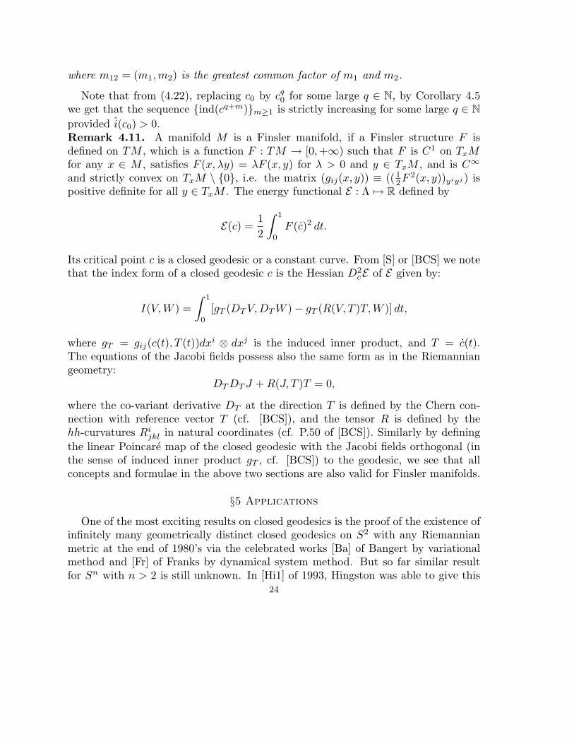
we get that the sequence ind(cq+m)m≥1 is strictly increasing for some large q ∈ Nprovided i(c0) > 0.Remark 4.11. A manifold M is a Finsler manifold, if a Finsler structure F isdefined on TM , which is a function F : TM → [0, +∞) such that F is C1 on TxMfor any x ∈ M , satisfies F (x, λy) = λF (x, y) for λ > 0 and y ∈ TxM , and is C∞

and strictly convex on TxM \ 0, i.e. the matrix (gij(x, y)) ≡ (( 12F 2(x, y))yiyj ) is

positive definite for all y ∈ TxM . The energy functional E : Λ 7→ R defined by

E(c) =12

∫ 1

0

F (c)2 dt.

Its critical point c is a closed geodesic or a constant curve. From [S] or [BCS] we notethat the index form of a closed geodesic c is the Hessian D2

cE of E given by:

I(V,W ) =∫ 1

0

[gT (DT V, DT W )− gT (R(V, T )T, W )] dt,

where gT = gij(c(t), T (t))dxi ⊗ dxj is the induced inner product, and T = c(t).The equations of the Jacobi fields possess also the same form as in the Riemanniangeometry:

DT DT J + R(J, T )T = 0,

where the co-variant derivative DT at the direction T is defined by the Chern con-nection with reference vector T (cf. [BCS]), and the tensor R is defined by thehh-curvatures Ri

jkl in natural coordinates (cf. P.50 of [BCS]). Similarly by definingthe linear Poincare map of the closed geodesic with the Jacobi fields orthogonal (inthe sense of induced inner product gT , cf. [BCS]) to the geodesic, we see that allconcepts and formulae in the above two sections are also valid for Finsler manifolds.

§5 Applications

One of the most exciting results on closed geodesics is the proof of the existence ofinfinitely many geometrically distinct closed geodesics on S2 with any Riemannianmetric at the end of 1980’s via the celebrated works [Ba] of Bangert by variationalmethod and [Fr] of Franks by dynamical system method. But so far similar resultfor Sn with n > 2 is still unknown. In [Hi1] of 1993, Hingston was able to give this

24

result a unified proof by variational method. Her contribution gives some hope forthe higher dimensional case. Our following Theorem 5.1 is related to Proposition Iof [Hi1] and the main theorem of [Hi2] of Hingston. We hope this result clarifies themeaning of certain conditions of Hingston in some sense via our iteration Theorems4.1, 4.4, 4.6, and 4.7, and help to further understand the results in [Ba], [Fr], [Hi1],and [Hi2].

Theorem 5.1. Let M be an n-dimensional compact Riemannian manifold, and c bea closed geodesic on M . Denote the length of c by l, the linear Poincare map of c byP , λ = ind(c), and η = null(c). Let Λl = α ∈ Λ | E(α) ≤ l2/2. Assume

(A) Hλ+η(Λl ∪ c,Λl) 6= 0,(B) I2p ¦N1(1,−1)¦(n−1−p) ∈ Ω0(P ), for some non-negative integer p,

or dually,(A’) Hλ(Λl ∪ c, Λl) 6= 0,(B’) I2p ¦N1(1, 1)¦(n−1−p) ∈ Ω0(P ), for some non-negative integer p.

Then M possesses infinitely many closed geodesics.

Proof. We prove the following two claims first.Claim 1. The condition (B) is equivalent to the following condition (2) of Propo-

sition I of [Hi1]:(2) ind(cq) + null(cq) ≤ q(ind(c) + null(c))− (q − 1)(n− 1), ∀q ∈ N.In fact, suppose (B) holds for some p ≥ 0. Then there holds null(cq) = null(c) =

n + p− 1, and by Theorem 4.7, for all q ∈ N, there holds

ind(cq) = q(ind(c) + p)− p

= q(ind(c) + null(c)− n + 1) + n− 1− null(c)

= q(ind(c) + null(c)− n + 1) + n− 1− null(cq). (5.1)

From (5.1) we obtain the above condition (2).Conversely, suppose the condition (2) holds. Then by the left inequality of (4.13)

in Theorem 4.6, the equality in the left hand side of (4.13) must hold for all q ∈ N.By (ii) of Theorem 4.6, we then obtain I2p ¦ N1(1,−1)¦(n−1−p) ∈ Ω0(P ) for somenon-negative integer p. That is the condition (B) in Theorem 5.1. Thus Claim 1holds.

Claim 2. The conditions (A’) and (B’) are equivalent to the following conditions(1’) and (2’) of the main Theorem of [Hi2]:

(1’) Hj(Λl ∪ c, Λl) 6= 0 for some j ∈ Z+.(2’) ind(cq) ≥ qj + (q − 1)(n− 1), ∀q ∈ N.

25

In fact, suppose (A’) and (B’) hold. Then (1’) holds for j = λ. By (B’) andTheorem 4.7, for all q ∈ N there hold null(cq) = null(c) = n + p− 1 and

ind(cq) = q(ind(c)+ p+n− 1− p)− p− (n− 1− p) = q ind(c)+ (q− 1)(n− 1). (5.2)

That is, (2’) holds with equality.Conversely, suppose (1’) and (2’) hold. Then by the critical point theory, we have

ind(c) ≤ j ≤ ind(c) + null(c). Thus by the right hand side inequality of (4.13) inTheorem 4.6, the equality in (2’) must hold, and j = ind(c). Thus the equality on theright hand side of (4.13) must hold for all q ∈ N. Then by (iii) of Theorem 4.6, thereholds I2p ¦N1(1, 1)¦(n−1−p) ∈ Ω0(P ) for some non-negative integer p. Therefore (A’)and (B’) in Theorem 5.1 hold. This completes the proof of Claim 2.

Now by these two claims, the conclusion of our theorem follows from PropositionI of [Hi1] and the main theorem of [Hi2]. ¤

Remark 5.2. By our proof of Theorem 5.1, the inequality conditions (2) and (2’) of[Hi1] and [Hi2] are actually requiring equalities and are two extreme cases in Theorem4.6.

References

[BTZ] Ballmann W,, Thorberrgsson G. and Ziller. W, Closed geodesics on positively curved man-ifolds, Annals of Math. 116 (1982), 213-247.

[Ba] Bangert V., On the existence of closed geodesics on two-spheres, Inter. J. of Math. 4 (1993),1-10.

[BCS] Bao D., Chern S.S. and Shen Z., An Introduction to Riemann-Finsler Geometry, Springer,2000.

[Bo1] Bott R., On the iteration of closed geodesics and the sturm intersection theory, Commun.Pure Appl. Math. 9 (1956), 171-206.

[Bo2] Bott R., Lectures on More theory, old and new, Bull. Amer. Math. Soc. 7(2) (1982),331-358.

[Fr] Franks J., Geodesics on S2 and periodic points of annulus homeomorphisms, Invent. Math.108 (1992), 403-418.

[GM] Gromoll D. & Meyer W., Periodic geodesics on compact Riemannian manifolds, J. Diff.Geom. 3 (1969), 493-510.

[Hi1] Hingston N., On the growth of the number of closed geodesics on the two-sphere, Inter.Math. Res. Notices 9 (1993), 253-262.

[Hi2] Hingston N., On the lengths of closed geodesics on a two-sphere, Proc. Amer. Math. Soc.125(10) (1997), 3099-3106.

[Kl] Klingenberg W., Riemannian Geometry, Walter de Gruyter, 1982.

[LL1] Liu C. and Long Y., Iteration inequalities of the Maslov-type index theory with applications,J. Diff. Equa. 165 (2000), 355-376.

26

[LL2] Liu C. and Long Y., An optimal increasing estimate of the iterated Maslov-type indices,Chinese Science Bulletin 42 (1997), 2275-2277.

[Lo1] Long Y., Bott formula of the Maslov-type index theory,, Pacific J. Math. 187 (1999), 113-149.

[Lo2] Long Y., Precise iteration formula of the Maslov-type index theory and ellipticity of closedcharacteristics, Advances in Math. 154 (2000), 76-131.

[LZ] Long Y. and Zhu C., Closed characteristics on compact convex hypersurfaces in R2n, NankaiInst. of Math. Preprint Series. No. 1999-M-002, Revised Dec. 2000, submitted.

[Mo] Morse M., The Calculus of Variations in the Large, vol. 18, Amer. Math. Soc. ColloquiumPubl., 1934.

[Rad] Rademacher H.-B., On the average indices of closed geodesics, J. Diff. Geom. 29 (1989),65-83.

[S] Shen Z., Lectures on Riemannian-Finsler Geometry, preprint, 2000.[YS] Yakubovich V. and Starzhinskii V., Linear Differential Equations with Perodic Ceofficints,

New York, John Wiley & Sons, 1975.[Zi] Ziller W., Geschlossene Geodatische auf global symmetrischen und homogenen Raumen,

Bonn. Math. Schr. Nr. 85, 1976.

27