A GCM SIMULATION OF HEAT WAVES, DRY SPELLS, AND THEIRRELATIONSHIPS TO CIRCULATION

RADAN HUTH 1, JAN KYSELÝ1,2 and LUCIE POKORNÁ1

1Institute of Atmospheric Physics, Boˇcní II 1401, 141 31 Praha 4, Czech RepublicE-mail: huth@ufa.cas.cz

2Department of Meteorology and Environment Protection, Charles University, V Holešoviˇckách 2,180 00 Praha 8, Czech Republic

Abstract. Heat waves and dry spells are analyzed (i) at eight stations in south Moravia (CzechRepublic), (ii) in the control ECHAM3 GCM run at the gridpoint closest to the study area, and(iii) in the ECHAM3 GCM run for doubled CO2 concentrations (scenario A) at the same gridpoint(heat waves only). The GCM outputs are validated both against individual station data and areallyrepresentative values. In the control run, the heat waves are too long, appear later in the year, peakat higher temperatures and their numbers are under- (over-) estimated in June and July (in August).The simulated dry spells are too long, and the annual cycle of their occurrence is distorted. Mid-tropospheric circulation, and heat waves and dry spells are linked much less tightly in the controlclimate than in the observed. Since mid-tropospheric circulation is simulated fairly successfully, wesuggest the hypothesis that either the air-mass transformation and local processes are too strong inthe model or the simulated advection is too weak. In the scenario A climate, the heat waves becomea common phenomenon: warming of 4.5◦C in summer (difference between scenario A and controlclimates) induces a five-fold increase in the frequency of tropical days and an immense enhancementof extremity of heat waves. The results of the study underline the need for (i) a proper validationof the GCM output before a climate impact study is conducted and (ii) translation of large-scaleinformation from GCMs into local scales using downscaling and stochastic modelling techniques inorder to reduce GCMs’ biases.

1. Introduction

Ecosystems and various sectors of human activities are particularly sensitive toextreme climate phenomena, including heavy rains, droughts, high and low tem-peratures. Even relatively small changes in means and variations of relevant climatevariables can induce considerable changes in the severity of extreme events (Katzand Brown, 1992; Hennessy and Pittock, 1995). Such changes are likely to have agreat impact on ecosystems and society. Of particular importance are long-lastingextreme events, such as prolonged periods with no precipitation (dry spells) andwith high temperatures (heat waves), both imposing high stress on plants, animalsand humans. Heat waves and dry spells are the focus of this study.

Among a variety of harmful effects, episodes of extremely high temperaturescan damage plants, especially when there is a shortage of water (Kirschbaum,1996), which can adversely affect their growth during key development stages

Climatic Change46: 29–60, 2000.© 2000Kluwer Academic Publishers. Printed in the Netherlands.

30 RADAN HUTH ET AL.

(Acock and Acock, 1993). Heat stress has detrimental effects also on livestockwith significant impacts on milk production, as well as on reproductive capabilitiesof dairy bulls and conception in cows (Thatcher, 1974; Cavestany et al., 1985;Furquay, 1989). Heat waves pose a danger for human health, too, and during heatwaves, the overall death rates rise (Kalkstein and Smoyer, 1993; Kunst et al., 1993;Changnon et al., 1996). The prolonged periods with no precipitation may causea soil moisture deficit, which impairs crops as consistent moisture availabilitythroughout the growth period is critical for them (Reilly, 1996).

General Circulation Model (GCM) studies have recently paid increased atten-tion to extreme phenomena, both in validating simulated present-day climates andanalyzing possible future climates. For example, Joubert et al. (1996) and Masonand Joubert (1997) analyzed frequencies of droughts and extreme rainfall events inSouth Africa in the CSIRO GCM. Hennessy et al. (1997) examined the probabilityof exceeding precipitation thresholds in two GCMs at various locations. Gregory etal. (1997) dealt with dry spells and their return periods in the transient experimentwith the Hadley Centre GCM.

The climate variables on a local scale are to a certain extent (widely differingamong variables) governed or influenced by large-scale circulation. The heat wavesand dry spells do not therefore occur independently of circulation conditions, buttheir occurrence is favoured by certain flow configurations while unlikely underother ones. The relationship between circulation and the occurrence of prolongedextreme events is thus an important component of a climate system, and the ac-curacy with which it is simulated by a GCM can serve as one of indicators ofthe model’s validity. For example, Risbey and Stone (1996) found that circulationconditions producing high precipitation events differ between the model and real-ity, precipitation being caused by different mechanisms. Heat waves and dry spellshave not been examined from this point of view yet.

The present paper investigates heat waves and dry spells observed in southMoravia (southeastern part of the Czech Republic) during the vegetation period,and their relationships with continental-scale circulation. The observations arecompared with the corresponding ECHAM GCM simulations both for presentclimate and for doubled CO2 concentrations.

When validating a GCM output on a local scale, one should bear in mind thatGCMs have not been designed for simulating local climate. The interpretation ofGCM outputs is, therefore, ambiguous: The values at GCM’s gridpoints can betreated in two alternative ways, either as areal or point quantities. In terms ofGCM validation, i.e., comparing simulated and observed values, this means thatGCM gridpoint values should be compared either with area-averaged observationsor directly with local values. There is continuing debate, about which approachshould be given preference and considered more appropriate, but still without adefinitive conclusion (Skelly and Henderson-Sellers, 1996; Zwiers and Kharin,1998). Some studies have compared GCM outputs with observations at individualstations (Portman et al., 1992; Palutikof et al., 1997; Schubert, 1998; Nemešová

A GCM SIMULATION 31

et al., 1998, to name a few), others with observations interpolated to gridpoints orwith gridded climatologies (e.g., Airey and Hulme, 1995; Risbey and Stone, 1996;Osborn and Hulme, 1998). The dilemma is perhaps more serious for precipitation,which is more spatially variable, and whose spatial behaviour widely changes fromseasons and regions with prevailing stratiform rainfall to those with convectiverainfall. Robinson et al. (1993) have shown that during the convective season, theGCM-simulated number of dry days closely approximated the individual stationvalues, whereas during the seasons with prevailing stratiform precipitation, it wascloser to the areal aggregate value.

Nevertheless, the approach to validation is frequently selected arbitrarily, whichis only sometimes explicitly admitted (e.g., by Osborn and Hulme, 1998). In thispaper, the GCM outputs are validated against the individual station values and twokinds of area-representative variables: (i) the ‘pooled’ ones obtained by averagingthe heat wave and dry spell characteristics, calculated at individual stations, and(ii) the ‘averaged’ or ‘aggregated’ ones, obtained by calculating the characteristicsfrom area-averaged or aggregated series. Whereas the pooled values can be thoughtof as characteristics at a ‘typical’ single station, the averaged (aggregated) valuesdescribe the behaviour of area-averaged temperature and precipitation, forming ananalogy to a GCM output treated as a gridbox value.

Recent examinations of the ECHAM GCM revealed that its precipitationclimatology is simulated worse than its temperature climatology in the regionconsidered. Specifically, the model systematically underestimates the interdiurnalvariability of temperature and is too wet (Nemešová and Kalvová, 1997; Kalvováand Nemešová, 1998; Nemešová et al., 1998).

2. Data

This study examines the heat waves and dry spells during the vegetation period,which in central Europe covers approximately the months from March to October.Three datasets are analyzed: observations, the ECHAM simulation of the presentclimate (control run; CTR), and the equilibrium ECHAM simulation of the climateunder doubled CO2 concentrations (scenario A run; SCA). The simulated datasetswere produced by the ECHAM3 model with the T42 resolution, correspondingapproximately to a 2.8◦ gridstep both in longitude and latitude. In the controlrun, the climatological SSTs and sea ice were employed while the scenario Aequilibrium run was forced by SSTs and sea ice averaged over years 65 to 74(roughly corresponding to doubling CO2) in the scenario A transient integration.The model is described in detail in DKRZ (1993). Each dataset comprises thirtyyears. Observations span the period 1961–1990; in the simulations, years 11 to 40in the control run and years 13 to 42 in the scenario run are analyzed. Each modelmonth consists of 30 days. The observations thus amount to 7350 days, and CTRand SCA data to 7200 days.

32 RADAN HUTH ET AL.

Figure 1. Location of stations used in the study (dots) and ECHAM GCM grid points (crosses).Stations are identified by their numbers, with their altitudes (in m a.s.l.) given in parentheses.

The observed maximum temperatures and precipitation are analyzed at eightsouth Moravian stations (Moravia is the eastern part of the Czech Republic). Fig-ure 1 shows their locations and altitudes together with the position of the closeECHAM gridpoints. Because of similarity of basic characteristics of simulatedtemperature and precipitation time series at the four close gridpoints (Kalvová andNemešová, 1998; Nemešová et al., 1998), point E4, nearest to the region analyzed,was taken as a representative of south Moravia in the model.

Continental-scale circulation is characterized by 500 hPa geopotential heights.The observed values were interpolated using bicubic splines from the 5◦ × 5◦ gridonto the model grid (approximately 2.8◦ × 2.8◦), covering most of Europe and

A GCM SIMULATION 33

the easternmost flank of the Atlantic Ocean. For the area covered by the grid, seeFigure 5 as an example.

3. Heat Waves

There are two general approaches to defining heat waves: Either the most extremeevents lasting the period of a required duration (typically one to three days) in eachsummer are selected or all heat waves above a certain threshold are analyzed (Karland Knight, 1997). Here we adopted the latter approach as it allows us to considerseveral heat waves in one year. Possible definitions of what can be considered aheat wave differ according to the thresholds employed, for example, in its requiredduration and extremity. We found it useful to define the heat wave as ‘the longestcontinuous period (i) during which the maximum daily temperature reached at leastT1 in at least three days, (ii) whose mean maximum daily temperature was at leastT1, and (iii) during which the maximum daily temperature did not drop below T2’.The threshold temperatures T1 and T2 are set to 30◦ and 25◦C, respectively, inobservations. This is in accordance with common climatological practice in theCzech Republic, which refers to the days with maximum temperature reaching orexceeding 30◦ and 25◦C as tropical and summer days, respectively. The definitionfollows the general perception of what a heat wave is: It allows two periods oftropical days separated by a slight drop of temperature to compose one heat wavebut, on the other hand, two periods of tropical days separated by a pronounced tem-perature drop below 25◦C (e.g., due to a cold front passage) are treated as separateheat waves. The minimum duration of a heat wave required by the definition isthree days.

Given the definition for observed data, there are two ways of defining the heatwave in the GCM control simulation. Either the thresholds of 30◦ and 25◦C canbe directly applied or the thresholds can be redefined in the control run so thatthe probability of exceeding them would be the same as in the observed. Thelatter way accounts for the model’s possible temperature bias, thereby allowinga more direct interpretation of the scenario run, and has therefore been applied inthis study. The respective percentiles of the maximum temperature distributionscorresponding to 30◦ and 25◦C thresholds were determined at the eight stationsfor the period from May to September. Their values representative for the regionwere obtained by averaging the eight local percentiles: They equal 97.1% and80.9%, respectively, for 30◦ and 25◦C temperatures. In the simulated maximumtemperature distribution at point E4, the two percentiles coincide with temperaturesof 30.7◦ and 24.5◦C. This procedure is referred to as ‘averaged-percentiles’ (AP)adjustment. An alternative to it is to take the time series of area-averaged values asa basis (‘averaged-temperature’ – AT adjustment): The areal mean temperature of30◦C and 25◦C corresponds to the percentiles of 97.7% and 82.0%, respectively, inits distribution; the adjusted threshold temperatures in the control simulation then

34 RADAN HUTH ET AL.

being 31.2◦C and 24.7◦C. Both ways of adjusting simulated thresholds lead to thevalues that correspond relatively well to the observed thresholds, indicating thatthe right tail of the maximum temperature distribution is simulated by the modelrather successfully, even though it is notably flatter relative to observations. In thetwo simulated climates, the terms ‘summer day’ and ‘tropical day’ refer to theadjusted threshold temperatures.

Basic characteristics of heat waves are summarized in Table I for individualstations and gridpoint E4. Also shown are the characteristics pooled over all thestations, and over the lowland and higher-elevated stations separately, as well asthe characteristics for the spatially averaged temperature series. The heat waves arecharacterized by their total occurrence in 30 years, average peak day (the peak dayis the central day of the three-day period with highest mean maximum temperaturewithin a particular heat wave), average duration, peak temperature (the highestmaximum temperature of a heat wave), relative position of the peak within the heatwave (defined as a ratio between the order of the peak day within the heat waveand its duration), and the percentage of all tropical days that occur in heat waves.

A detailed scrutiny of the observed heat waves was performed by Kyselý andKalvová (1998). Here we only note a pronounced dependence of several charac-teristics on elevation: at higher elevations, the heat waves are less frequent, tend topeak later and to be shorter, and the percentage of tropical days that occur in heatwaves is smaller. The peak temperature and the relative position of the peak appearto be independent of elevation. The heat wave characteristics calculated from theaveraged temperature series (AVG) closely resemble the characteristics averagedover individual stations (ALL). The only exception is the relative position of theheat wave peak, which in the averaged temperatures is shifted to the center of heatwaves.

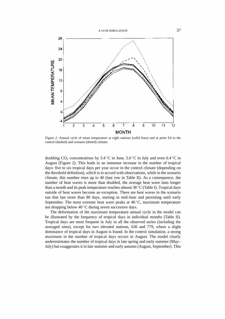
The AT adjustment results in a bit higher threshold temperatures, so the two ad-justments lead to slightly different heat wave characteristics in the control climate:the mean duration is shorter and peak temperature higher for the AT adjustment.The most important finding is, however, a disparity between the control and ob-served heat wave characteristics, regardless of how they are defined. The heat wavefrequency and the relative position of the peak in the control simulation comparequite well with the observations; however, these are the only two quantities that arereproduced successfully by the model. The simulated heat waves are much longerthan the observed, tend to occur later, and peak at temperatures by about 2◦Chigher. Also, fewer tropical days occur outside of heat waves. Most of these dis-crepancies result from two shortcomings of the model, viz., too low an interdiurnalvariability (Nemešová and Kalvová, 1997) and a deformation of the temperatureannual cycle with a maximum shifted towards August (see Figure 2 where theannual cycles of the mean temperature are shown for the eight stations and twomodel runs).

The character of heat waves changes dramatically in the scenario climate. Themodel indicates that the mean monthly temperature at point E4 increases due to

AG

CM

SIM

UL

AT

ION

35

TABLE I

Characteristics of heat waves: total number in 30 years; average peak day (day/month), duration (days), peak temperature (◦C), and relative position of thepeak within the heat wave (ratio between the order of the peak day within the heat wave and its duration); and the percentage of tropical days that occur inheat waves. Values are given for individual stations (636 to 779), pooled over lowland (LO), higher-elevated (HI) and all (ALL) stations, for spatially averagedtemperature (AVG), and for the control (CTR) and scenario (SCA) climates at point E4. The higher-elevated stations are 636, 687 and 779, the lowland stationsinclude the other five. The values for simulated climates are shown for both threshold adjustments (AP and AT – see text for definitions)

636 687 698 723 754 755 774 779 LO HI ALL AVG CTR CTR SCA SCA

AP AT AP AT

Number 9 16 28 32 37 43 30 11 34 12 26 22 24 22 53 52

Peak day 4/8 25/7 27/7 30/7 24/7 25/7 26/7 1/8 26/7 31/7 28/7 30/7 9/8 8/8 3/8 5/8

Duration 5.3 5.9 7.8 7.2 7.4 6.8 6.4 5.3 7.1 5.5 6.5 6.6 11.3 9.7 34.8 33.7

Peak temp. 32.9 32.7 33.3 32.5 32.8 32.6 32.4 32.0 32.7 32.5 32.6 32.5 34.4 34.7 37.8 37.9

Position 0.76 0.63 0.68 0.71 0.63 0.63 0.67 0.60 0.66 0.66 0.66 0.59 0.62 0.62 0.58 0.57

Percentage 39.5 42.7 57.3 63.0 63.3 66.1 59.6 43.3 62.2 42.0 58.0 58.4 82.3 81.0 97.4 97.1

36R

AD

AN

HU

TH

ET

AL

.

TABLE II

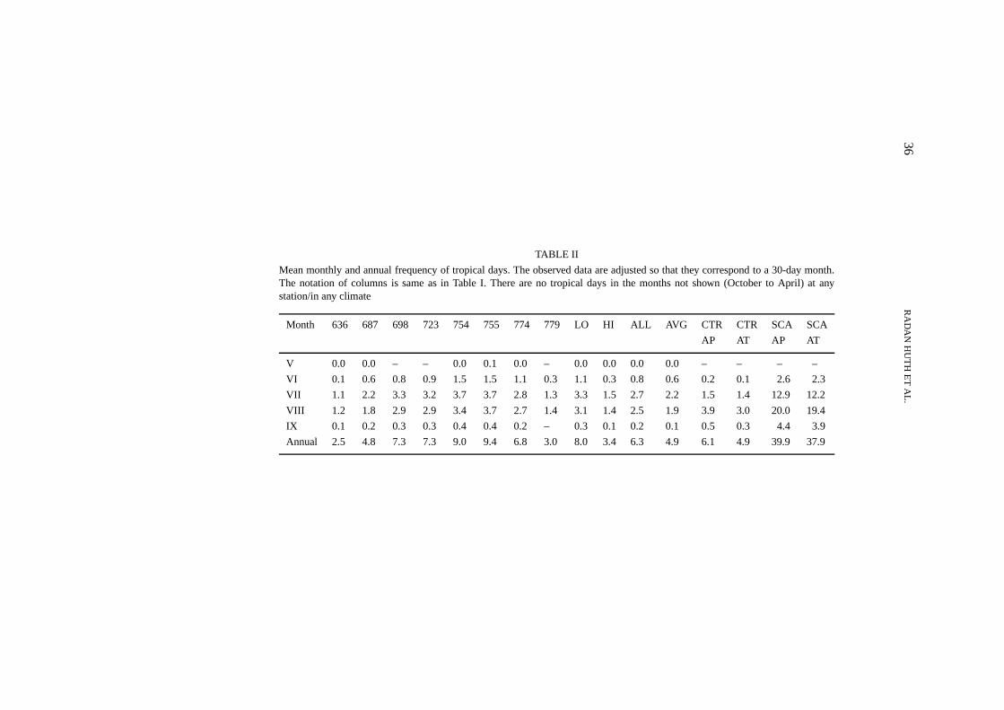
Mean monthly and annual frequency of tropical days. The observed data are adjusted so that they correspond to a 30-day month.The notation of columns is same as in Table I. There are no tropical days in the months not shown (October to April) at anystation/in any climate

Month 636 687 698 723 754 755 774 779 LO HI ALL AVG CTR CTR SCA SCA

AP AT AP AT

V 0.0 0.0 – – 0.0 0.1 0.0 – 0.0 0.0 0.0 0.0 – – – –

VI 0.1 0.6 0.8 0.9 1.5 1.5 1.1 0.3 1.1 0.3 0.8 0.6 0.2 0.1 2.6 2.3

VII 1.1 2.2 3.3 3.2 3.7 3.7 2.8 1.3 3.3 1.5 2.7 2.2 1.5 1.4 12.9 12.2

VIII 1.2 1.8 2.9 2.9 3.4 3.7 2.7 1.4 3.1 1.4 2.5 1.9 3.9 3.0 20.0 19.4

IX 0.1 0.2 0.3 0.3 0.4 0.4 0.2 – 0.3 0.1 0.2 0.1 0.5 0.3 4.4 3.9

Annual 2.5 4.8 7.3 7.3 9.0 9.4 6.8 3.0 8.0 3.4 6.3 4.9 6.1 4.9 39.9 37.9

A GCM SIMULATION 37

Figure 2. Annual cycle of mean temperature at eight stations (solid lines) and at point E4 in thecontrol (dashed) and scenario (dotted) climate.

doubling CO2 concentrations by 3.4◦C in June, 5.6◦C in July and even 6.4◦C inAugust (Figure 2). This leads to an immense increase in the number of tropicaldays: five to six tropical days per year occur in the control climate (depending onthe threshold definition), which is in accord with observations, while in the scenarioclimate, this number rises up to 40 (last row in Table II). As a consequence, thenumber of heat waves is more than doubled, the average heat wave lasts longerthan a month and its peak temperature reaches almost 38◦C (Table I). Tropical daysoutside of heat waves become an exception. There are heat waves in the scenariorun that last more than 80 days, starting in mid-June and persisting until earlySeptember. The most extreme heat wave peaks at 46◦C, maximum temperaturenot dropping below 40◦C during seven successive days.

The deformation of the maximum temperature annual cycle in the model canbe illustrated by the frequency of tropical days in individual months (Table II).Tropical days are most frequent in July in all the observed series (including theaveraged ones), except for two elevated stations, 636 and 779, where a slightdominance of tropical days in August is found. In the control simulation, a strongmaximum in the number of tropical days occurs in August. The model clearlyunderestimates the number of tropical days in late spring and early summer (May–July) but exaggerates it in late summer and early autumn (August, September). This

38 RADAN HUTH ET AL.

TABLE III

Mean monthly and annual frequency of tropical days in heat waves. Thevalues for individual stations are not shown; otherwise as in Table II

Month LO HI ALL AVG CTR CTR SCA SCA

AP AT AP AT

V – – – – – – – –

VI 0.5 0.1 0.4 0.1 0.2 0.1 2.3 1.9

VII 2.3 0.7 1.7 1.5 1.2 1.1 12.6 11.9

VIII 2.0 0.6 1.4 1.1 3.1 2.6 19.8 19.2

IX 0.1 0.1 0.1 0.1 0.5 0.2 4.2 3.7

Annual 5.0 1.4 3.6 2.8 5.0 4.0 38.9 36.8

unrealistic feature, i.e., the shift of the annual temperature maximum to August, isretained in the scenario run: the number of tropical days in August highly exceedsthat in July.

Despite the deformation of the seasonal cycle, the heat waves occur in thesame months in the control run as in observations, i.e., in June to September(Table III). An interesting feature is that although the thermal extremity increasesin the scenario run in all aspects (number of tropical days, number and duration ofheat waves), the heat waves do not spread further to spring and autumn and theiroccurrence remains limited to the period from June to September.

The conclusions concerning the simulated heat waves do not appear to besensitive to what they are compared with: both the characteristics of the spatiallyaveraged temperature and the pooled characteristics yield similar results, whichdiffer widely from the control simulation. Most characteristics of control heatwaves fall well outside the range of values observed at individual stations. On theother hand, the results for the control climate are robust regarding the definition ofthreshold temperatures. In other words, the validation of heat waves appears to beinsensitive to whether the GCM output is treated as gridpoint or gridbox value.

4. Dry Spells

Dry spells are usually defined as runs of consecutive days without precipitation.In many applications, however, it is common to allow days with very small pre-cipitation amounts to be considered as dry and to be included in dry spells (e.g.,Joubert et al., 1996; Gregory et al., 1997). In this study, we define a dry spell as thelongest continuous period lasting 10 days or more, during which the precipitationtotal does not exceed 1 mm.

A GCM SIMULATION 39

Figure 3. Annual cycle of monthly precipitation totals at eight stations (solid lines), their arealaverage (dotted), and at point E4 in the control climate (dashed).

Because of large spatial variability, constructing areal representation (aggregatevalue) of precipitation is a difficult task. Following Robinson et al. (1993), the‘aggregate dry day’ can be defined as the day when no precipitation was recordedat any station. This is a rather stringent definition, especially during the convectiveseason when local showers that are recorded at only a single station may be quitefrequent. Therefore, we employ another, more liberal, criterion, whereby we countdays with precipitation recorded at just one station as ‘aggregate dry days’. Thetwo criteria are referred to as ‘aggregate (0)’ and ‘aggregate (1)’, respectively, inthe text below.

To be able to calculate ‘aggregate dry spells’, one has to define the area-averaged precipitation series. Here, we define it simply as an average of stationvalues.

The analysis is confined to the observed and control climates, since for thescenario climate, precipitation values were unfortunately not available.

Let us start with monthly precipitation sums. There is a wide difference inannual cycle between the observed and control climate, the latter appearing to beunrealistic (Figure 3). The observed precipitation series agree with each other inhaving their annual maximum in early summer and minimum in winter; a sec-ondary minimum and maximum appear in October and November, respectively.The control annual cycle is clearly bimodal with maxima in June and Decemberand main minimum in August and September. The annual precipitation sum is

40 RADAN HUTH ET AL.

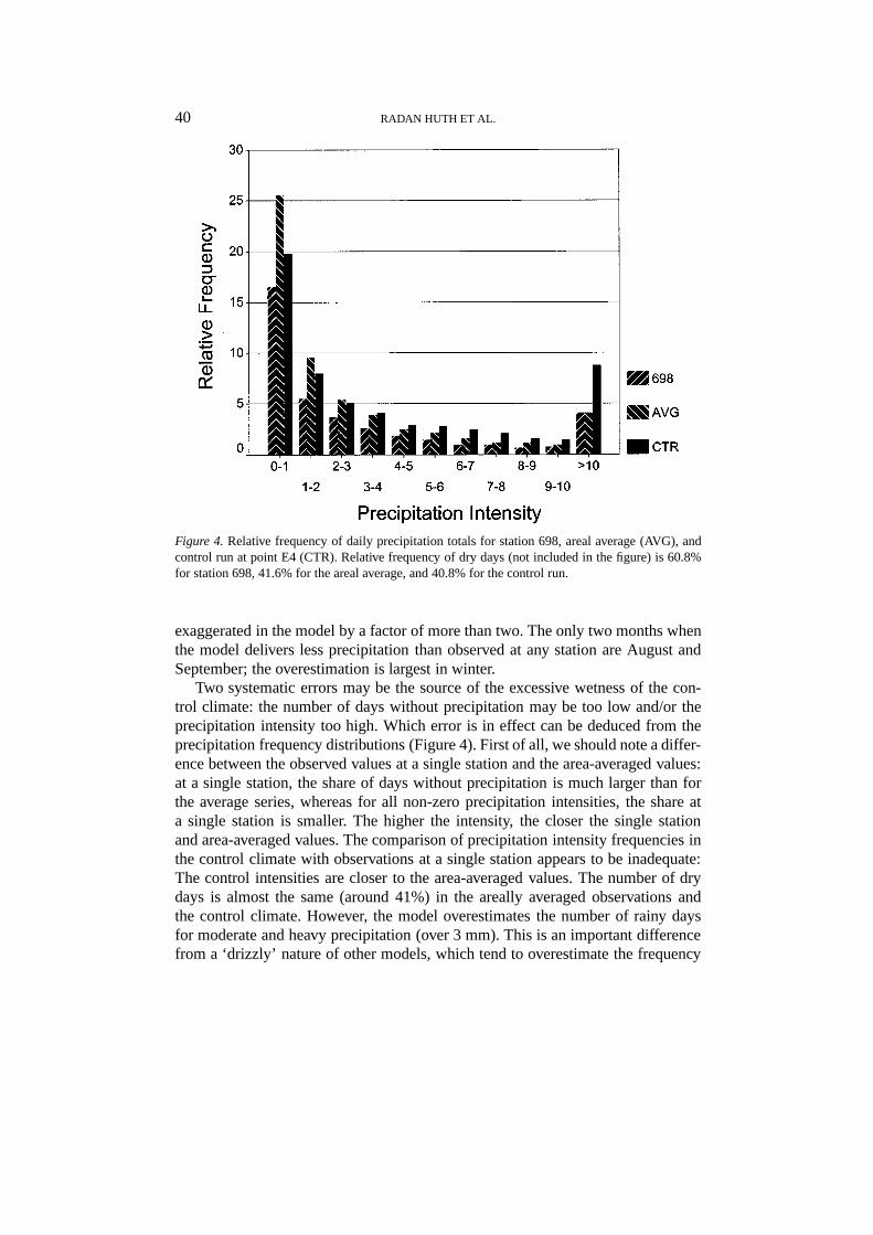
Figure 4.Relative frequency of daily precipitation totals for station 698, areal average (AVG), andcontrol run at point E4 (CTR). Relative frequency of dry days (not included in the figure) is 60.8%for station 698, 41.6% for the areal average, and 40.8% for the control run.

exaggerated in the model by a factor of more than two. The only two months whenthe model delivers less precipitation than observed at any station are August andSeptember; the overestimation is largest in winter.

Two systematic errors may be the source of the excessive wetness of the con-trol climate: the number of days without precipitation may be too low and/or theprecipitation intensity too high. Which error is in effect can be deduced from theprecipitation frequency distributions (Figure 4). First of all, we should note a differ-ence between the observed values at a single station and the area-averaged values:at a single station, the share of days without precipitation is much larger than forthe average series, whereas for all non-zero precipitation intensities, the share ata single station is smaller. The higher the intensity, the closer the single stationand area-averaged values. The comparison of precipitation intensity frequencies inthe control climate with observations at a single station appears to be inadequate:The control intensities are closer to the area-averaged values. The number of drydays is almost the same (around 41%) in the areally averaged observations andthe control climate. However, the model overestimates the number of rainy daysfor moderate and heavy precipitation (over 3 mm). This is an important differencefrom a ‘drizzly’ nature of other models, which tend to overestimate the frequency

A GCM SIMULATION 41

of light precipitation but underestimate heavier rains (e.g., Reed, 1986; Risbey andStone, 1996).

Basic characteristics of the distribution of dry spells duration (mean, median,maximum) as well as their mean annual frequency and the percentage of dry daysthat occur in dry spells are listed in Table IV. Shown are the values for the eightstations, values averaged over the lowland, higher-elevated and all stations, the val-ues for the area-averaged precipitation, and values for the control climate at pointE4. There is little difference in the characteristics of dry spells duration (mean,median, maximum) between individual stations and the area-averaged values, andbetween lowland and highland stations. For the area-averaged precipitation, theannual frequency of dry spells is much lower than at individual stations, and thereis much weaker tendency for dry days to chain in prolonged spells. It is also worthnoting that at lowland stations, the dry spells are more frequent and relatively moredays occur within dry spells than at higher-elevated stations. In the control climate,dry spells are longer than in the observed. Since the dry spells duration distributionsfor the observed and control climate have the same median but differ in their means,we can state that the model overestimates the frequency of very long spells at theexpense of spells with medium duration (13 to 20 days). The frequency of dryspells in the control climate compares fairly well with the observed area-averagedprecipitation; on the other hand, the simulated percentage of dry days occurringwithin dry spells resembles the single station values.

The observed and control climates differ notably in the distribution of dry daysand dry spells throughout the year. In the observed, the number of days withindry spells (Table V) closely reflects the annual cycle of precipitation: the largerthe precipitation total, the fewer days within dry spells. This holds both for area-averaged precipitation, and precipitation at individual stations, represented by thepooled values. In the control climate, such a simple relationship does not hold.The number of days within dry spells peaks in the driest months of August andSeptember, which corresponds to the minimum of the precipitation annual cycle.However, dry spells are rarest in spring even though March, April and May areall less wet than the month with maximum precipitation, i.e., June. Although theMarch and April precipitation amounts are comparable with July and October, thedry spells in spring are much less frequent. The total simulated frequency of drydays in the vegetation period (Table VI) is closest to the number of aggregate drydays according to criterion (1) (which allows the day with precipitation at onestation to be counted as dry). However, the annual cycles are very different: Thefrequency of dry days varies rather moderately in the observed, with the minimumin June and maximum in October. In the control climate, the range is much broader:dry days are least frequent in March (although March is far from being the wettestmonth) with less than six dry days on average whereas more than 21 dry days occurin August and September.

The percentage of dry days occurring in dry spells is almost the same in thecontrol climate as at individual stations if the vegetation period is considered as

42R

AD

AN

HU

TH

ET

AL

.

TABLE IV

Characteristics of dry spells: mean, median and maximum duration, mean annual frequency, and percentage of all dry days that occur in dryspells. Given are values for eight individual stations, the values pooled over five lowland (LO), three higher-elevated (HI), and all (ALL)stations, the values for precipitation series averaged over lowland, higher-elevated, and all stations, and the values for the control run. For thearea-averaged precipitation, the percentage is calculated for the aggregate dry days according to criterion (0), i.e., with no precipitation at anystation

Stations Pooled Averaged CTR

636 687 698 723 754 755 774 779 LO HI ALL LO HI ALL

Mean 13.8 14.1 14.8 14.6 14.5 14.9 13.8 14.0 14.5 14.0 14.3 14.2 14.0 13.7 18.1

Median 13 12 13 13 13 13 12 12 13 12 13 12 12 12 13

Maximum 34 36 34 38 38 38 31 34 36 38 38 35 34 34 49

Frequency 4.2 4.0 5.0 5.7 5.0 4.9 4.7 4.7 5.1 4.3 4.8 4.0 2.9 3.1 2.8

Percentage 38.1 37.6 45.1 48.6 45.7 44.5 41.9 38.2 45.2 38.0 42.6 24.9 20.0 22.0 42.5

A GCM SIMULATION 43

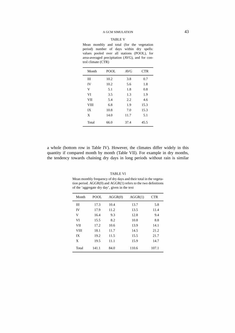
TABLE V

Mean monthly and total (for the vegetationperiod) number of days within dry spells:values pooled over all stations (POOL), forarea-averaged precipitation (AVG), and for con-trol climate (CTR)

Month POOL AVG CTR

III 10.2 3.8 0.7

IV 10.2 5.6 1.8

V 5.1 1.8 0.8

VI 3.5 1.3 1.9

VII 5.4 2.2 4.6

VIII 6.8 1.9 15.3

IX 10.8 7.0 15.3

X 14.0 11.7 5.1

Total 66.0 37.4 45.5

a whole (bottom row in Table IV). However, the climates differ widely in thisquantity if compared month by month (Table VII). For example in dry months,the tendency towards chaining dry days in long periods without rain is similar

TABLE VI

Mean monthly frequency of dry days and their total in the vegeta-tion period. AGGR(0) and AGGR(1) refers to the two definitionsof the ‘aggregate dry day’, given in the text

Month POOL AGGR(0) AGGR(1) CTR

III 17.3 10.4 13.7 5.8

IV 17.9 11.2 13.5 11.4

V 16.4 9.3 12.8 9.4

VI 15.5 8.2 10.8 8.8

VII 17.2 10.6 13.9 14.1

VIII 18.1 11.7 14.5 21.2

IX 19.2 11.5 15.5 21.7

X 19.5 11.1 15.9 14.7

Total 141.1 84.0 110.6 107.1

44 RADAN HUTH ET AL.

TABLE VII

Percentage of dry days occurring in dry spells, monthly values.Otherwise as in Table VI

Month POOL AGGR(0) AGGR(1) CTR

III 59.0 37.6 33.4 12.1

IV 57.0 36.2 32.6 15.8

V 31.1 14.7 12.7 8.5

VI 22.6 11.9 10.5 21.6

VII 31.4 16.9 14.1 32.6

VIII 37.6 12.4 12.4 72.2

IX 56.2 41.0 38.6 70.5

X 71.8 56.8 56.7 34.7

in the control climate (August and September) to the observed in October butconsiderably stronger than in the observed in spring (March and April).

5. Circulation

Before validating relationships of heat waves and dry spells to continental-scalecirculation, we should examine circulation itself. In doing so, we follow the meth-odology used in Huth (1997a) where continental-scale circulation is characterizedin two complementary ways, namely, by modes of variability and by circulationtypes.

Modes of variability are identified in two important frequency bands: (i)synoptic frequencies, in which synoptic-scale pressure formations (cyclones, an-ticyclones), affecting in midlatitudes the instantaneous weather conditions andtheir day-to-day changes, develop and move, and (ii) low frequencies, in whichplanetary-scale formations such as blocking events evolve, affecting weather con-ditions over large areas for relatively long time periods. For this purpose, 500 hPaheights were filtered using Blackmon and Lau’s (1980) low-pass and band-passfilters, which retain periods longer than 10 days (low frequencies) and 2.5 to 6 days(synoptic frequencies), respectively. As an analysis tool, obliquely rotated principalcomponent analysis (PCA) in an S-mode is used. The procedure is basically thesame as in Huth (1997a) where it is described in detail.

The modes of variability identified in the three datasets are displayed in Figures5 (low frequencies) and 6 (synoptic frequencies) in terms of principal component(PC) loadings. PC loadings are correlations of PC amplitudes with original (low-passed or band-passed) data. Circulation on each day in respective frequency bandscan be approximated by a linear combination of the modes detected. For example,

A GCM SIMULATION 45

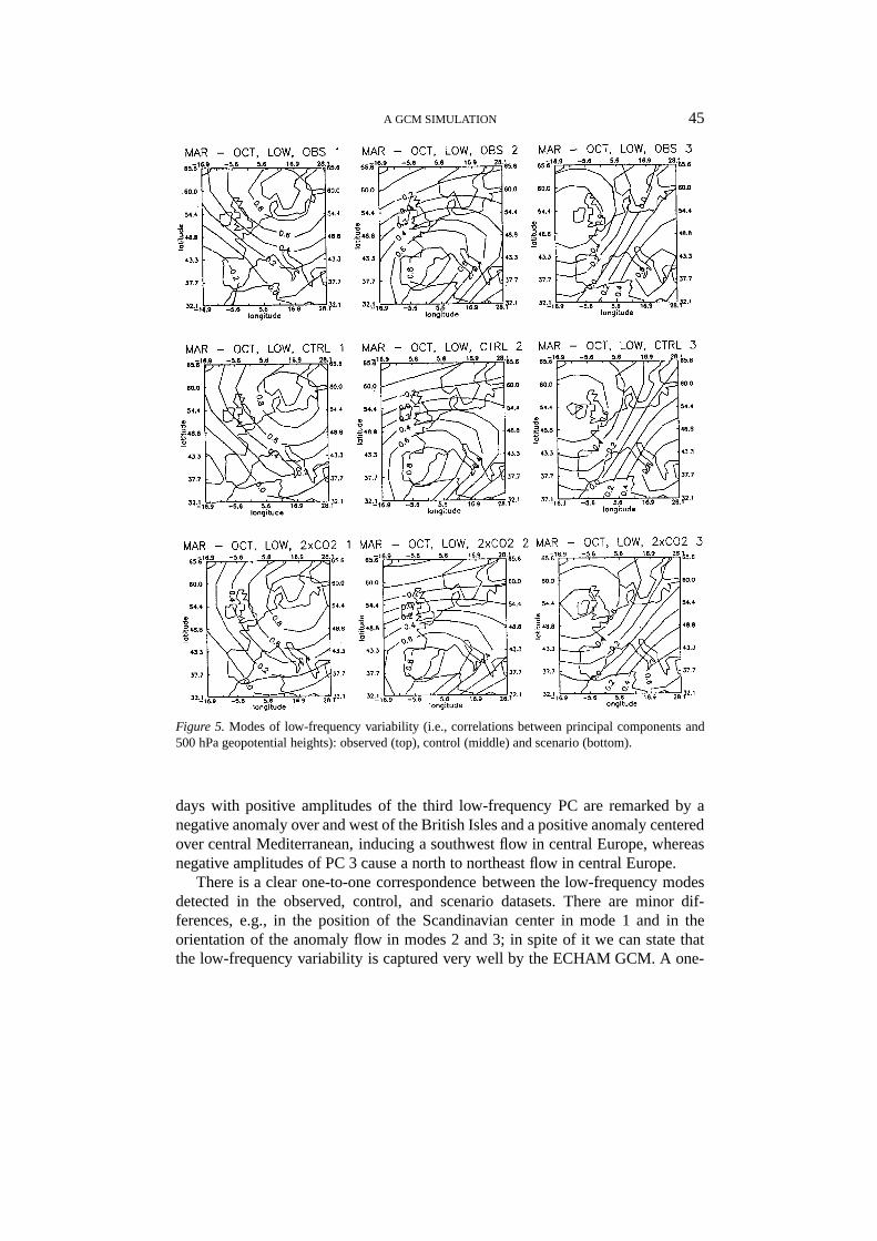
Figure 5.Modes of low-frequency variability (i.e., correlations between principal components and500 hPa geopotential heights): observed (top), control (middle) and scenario (bottom).

days with positive amplitudes of the third low-frequency PC are remarked by anegative anomaly over and west of the British Isles and a positive anomaly centeredover central Mediterranean, inducing a southwest flow in central Europe, whereasnegative amplitudes of PC 3 cause a north to northeast flow in central Europe.

There is a clear one-to-one correspondence between the low-frequency modesdetected in the observed, control, and scenario datasets. There are minor dif-ferences, e.g., in the position of the Scandinavian center in mode 1 and in theorientation of the anomaly flow in modes 2 and 3; in spite of it we can state thatthe low-frequency variability is captured very well by the ECHAM GCM. A one-

46 RADAN HUTH ET AL.

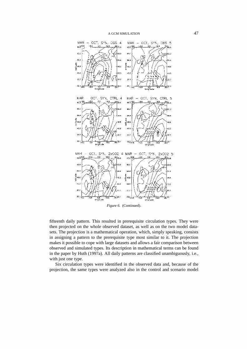
Figure 6.Modes of synoptic-frequency variability; otherwise as in Figure 5.

to-one correspondence can also be found for synoptic-frequency modes, that is,the variability in synoptic band is also well simulated by the model. (Note thatobserved mode 3 is paired with control and scenario mode 4, and vice versa.)The modes of variability in both frequency bands differ negligibly between thecontrol and scenario climates. This indicates that the enhanced greenhouse effectwill, according to the ECHAM GCM, cause only a marginal change in the modesof variability.

In identifying circulation types, we followed a modified methodology of Huth(1997a); please refer therein for more details on the procedures used. The PCAin a T-mode was applied to a subset of the observed dataset, consisting of every

A GCM SIMULATION 47

Figure 6. (Continued).

fifteenth daily pattern. This resulted in prerequisite circulation types. They werethen projected on the whole observed dataset, as well as on the two model data-sets. The projection is a mathematical operation, which, simply speaking, consistsin assigning a pattern to the prerequisite type most similar to it. The projectionmakes it possible to cope with large datasets and allows a fair comparison betweenobserved and simulated types. Its description in mathematical terms can be foundin the paper by Huth (1997a). All daily patterns are classified unambiguously, i.e.,with just one type.

Six circulation types were identified in the observed data and, because of theprojection, the same types were analyzed also in the control and scenario model

48 RADAN HUTH ET AL.

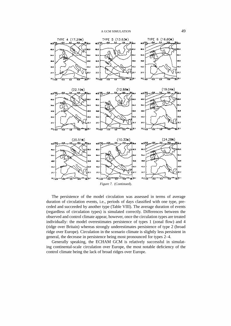
Figure 7.Mean 500 hPa height patterns (in metres) of the circulation types: observed (top), control(middle) and scenario (bottom). The percentage of occurrence of each type is given in parentheses.

runs. The mean 500 hPa height patterns for all the types in the three datasetsare shown in Figure 7. Several features are worth noting. First, some types aresimulated with incorrect frequency: the types 1 (zonal flow), 4 (ridge over Britain)and 6 (jet displaced far northwards) are too frequent in the model, whereas thefrequency of type 2 (broad ridge over Europe) is strongly underestimated. Second,some simulated types have slightly distorted patterns, e.g., the trough of type 3is too weak in the control climate. Analogous differences can be found betweenthe control and scenario climates, the most striking features being the increasedfrequency of days with jet displaced northwards (type 6) and decreased frequencyof troughs over western Europe (type 3).

A GCM SIMULATION 49

Figure 7. (Continued).

The persistence of the model circulation was assessed in terms of averageduration of circulation events, i.e., periods of days classified with one type, pre-ceded and succeeded by another type (Table VIII). The average duration of events(regardless of circulation types) is simulated correctly. Differences between theobserved and control climate appear, however, once the circulation types are treatedindividually: the model overestimates persistence of types 1 (zonal flow) and 4(ridge over Britain) whereas strongly underestimates persistence of type 2 (broadridge over Europe). Circulation in the scenario climate is slightly less persistent ingeneral, the decrease in persistence being most pronounced for types 2–4.

Generally speaking, the ECHAM GCM is relatively successful in simulat-ing continental-scale circulation over Europe, the most notable deficiency of thecontrol climate being the lack of broad ridges over Europe.

50 RADAN HUTH ET AL.

TABLE VIII

Average duration of circulation events (days) in observed (OBS),control (CTR) and scenario (SCA) climates: regardless of circulationtypes (ALL), and for individual types separately (1–6)

ALL 1 2 3 4 5 6

OBS 2.7 2.7 3.1 2.4 2.6 2.5 2.4

CTR 2.7 3.0 2.3 2.4 2.9 2.7 2.6

SCA 2.5 2.8 2.0 1.9 2.4 2.5 2.6

TABLE IX

Mean amplitudes of low-frequency circulation modes under heat waves. Shown arethe minimum (MIN) and maximum (MAX) value from the eight stations, the value forthe area-averaged temperature (AVG), and values for the control (CTR) and scenario(SCA) climates for the two threshold definitions (AP, AT)

Mode MIN MAX AVG CTR CTR SCA SCA

AP AT AP AT

1 0.582 0.813 0.701 0.347 0.336 0.144 0.155

2 0.375 0.576 0.466 0.118 0.187 0.080 0.085

3 0.184 0.333 0.323 0.273 0.297 0.042 0.041

6. Relationships between Heat Waves, Dry Spells and Circulation

In this section, we investigate which circulation conditions are associated with theoccurrence of prolonged extreme events, and which conditions act against theirformation. Heat waves and dry spells are related to circulation in two ways: First,the amplitudes of the circulation modes in both frequency bands are averaged overall the heat waves and dry spells. Second, the numbers of days in heat waves anddry spells are counted for individual circulation types separately. Indeed, causationcannot be proved this way. On the time scales discussed, however, one may assumethat in general, circulation governs surface weather, although the opposite effect isalso possible: For example, long-lasting high temperatures may support ridging inmid-troposphere.

6.1. MODES OF VARIABILITY

The observed heat waves are associated with positive amplitudes of all three low-frequency modes, the relationship with mode 1 being most intense as indicated byhighest mean amplitudes (Table IX). This holds for individual stations as well as

A GCM SIMULATION 51

TABLE X

Same as in Table IX except for synoptic-frequency modes

Mode MIN MAX CTR SCA

AP AP

1 0.044 0.100 0.024 –0.003

2 –0.069 –0.017 –0.035 –0.010

3 –0.104 0.011 –0.031 0.001

4 –0.030 0.031 0.003 –0.004

5 –0.010 0.064 0.054 0.010

the area-averaged series. This means that conditions favourable for a heat waveto occur in south Moravia are positive 500 hPa height anomalies over southernScandinavia (mode 1), southwest Europe (mode 2), and to a smaller extent overGreece and negative anomaly over Ireland (mode 3) (see Figure 5). This could beexpected since all these conditions support an inflow of warm air from south andsouthwest into central Europe (modes 1 and 3) and/or the presence of a ridge oranticyclone over there (modes 1 and 2).

The linkage between low-frequency modes and heat waves in the control cli-mate is considerably weaker. The effect of the Scandinavian anomaly (mode 1) isapproximately halved and that of southwest-European anomaly (mode 2) becomesnegligible. Only the relationship of mode 3 with heat waves is simulated with acorrect intensity. The influence of circulation modes becomes negligible in thescenario climate because of an immense increase in heat waves occurrence.

The synoptic-frequency modes do not manifest any relation to the occurrenceof heat waves (Table X). No effect of the synoptic-frequency modes appears in thecontrol and scenario climates either.

The linkage with modes of variability is weaker for dry spells than for heatwaves (Table XI). The only mode associated with the occurrence of dry spellsis low-frequency mode 1, whose positive amplitude inhibits precipitation due toforming a ridge or anticyclone over central Europe. This link is pronounced morestrongly for the area-averaged precipitation than at individual stations, but is re-produced too weak in the control climate. The synoptic-frequency modes haveno effect on dry spells, the mean amplitudes not exceeding 0.05 in either climateanalyzed (not shown).

6.2. CIRCULATION TYPES

The connection between circulation types and prolonged extreme events may becharacterized by a ratio between the number of event-days (i.e., days within theheat waves or dry spells) classified with a particular type and the total number

52 RADAN HUTH ET AL.

TABLE XI

Same as in Table IX except for dry spells

Mode MIN MAX AVG CTR

1 0.314 0.546 0.658 0.269

2 0.088 0.194 0.159 0.128

3 –0.052 0.112 –0.140 –0.080

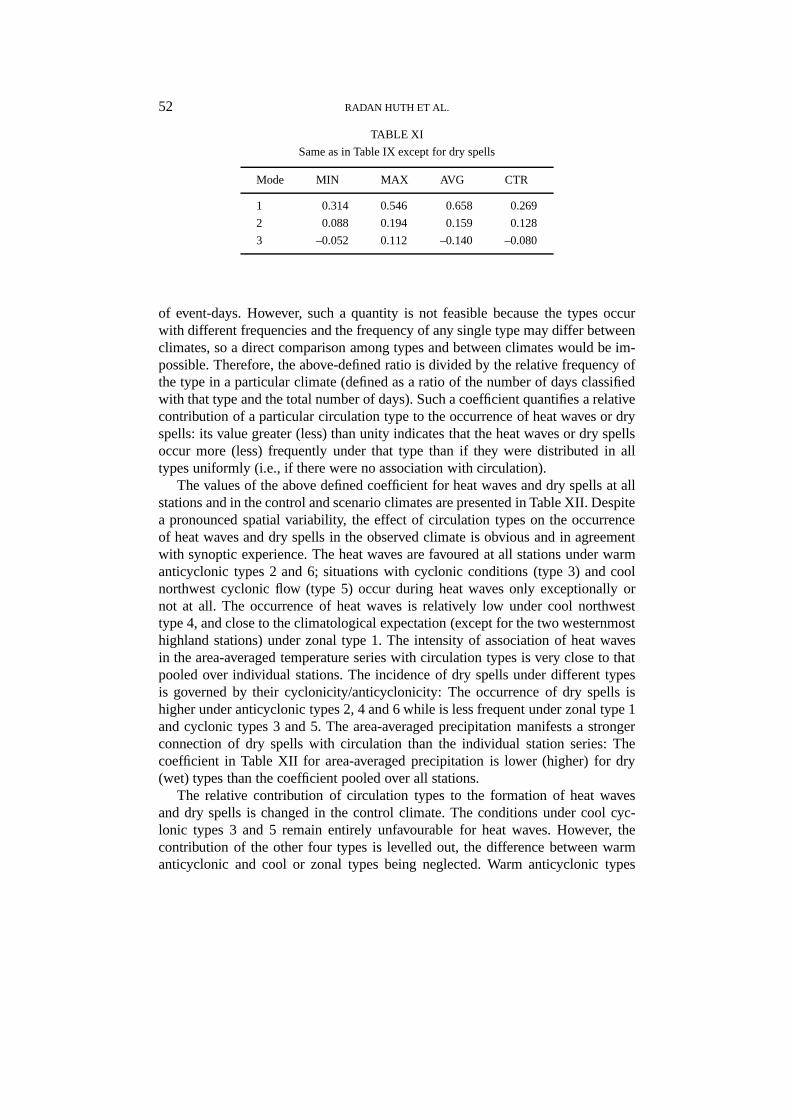
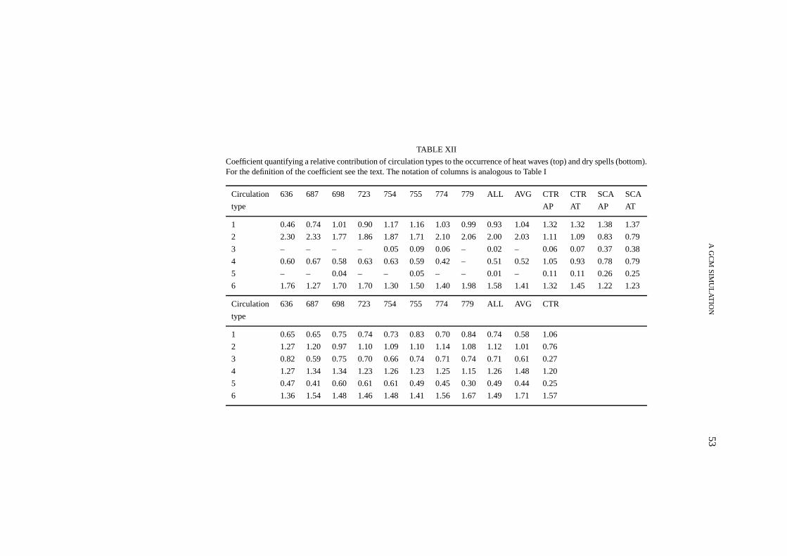
of event-days. However, such a quantity is not feasible because the types occurwith different frequencies and the frequency of any single type may differ betweenclimates, so a direct comparison among types and between climates would be im-possible. Therefore, the above-defined ratio is divided by the relative frequency ofthe type in a particular climate (defined as a ratio of the number of days classifiedwith that type and the total number of days). Such a coefficient quantifies a relativecontribution of a particular circulation type to the occurrence of heat waves or dryspells: its value greater (less) than unity indicates that the heat waves or dry spellsoccur more (less) frequently under that type than if they were distributed in alltypes uniformly (i.e., if there were no association with circulation).

The values of the above defined coefficient for heat waves and dry spells at allstations and in the control and scenario climates are presented in Table XII. Despitea pronounced spatial variability, the effect of circulation types on the occurrenceof heat waves and dry spells in the observed climate is obvious and in agreementwith synoptic experience. The heat waves are favoured at all stations under warmanticyclonic types 2 and 6; situations with cyclonic conditions (type 3) and coolnorthwest cyclonic flow (type 5) occur during heat waves only exceptionally ornot at all. The occurrence of heat waves is relatively low under cool northwesttype 4, and close to the climatological expectation (except for the two westernmosthighland stations) under zonal type 1. The intensity of association of heat wavesin the area-averaged temperature series with circulation types is very close to thatpooled over individual stations. The incidence of dry spells under different typesis governed by their cyclonicity/anticyclonicity: The occurrence of dry spells ishigher under anticyclonic types 2, 4 and 6 while is less frequent under zonal type 1and cyclonic types 3 and 5. The area-averaged precipitation manifests a strongerconnection of dry spells with circulation than the individual station series: Thecoefficient in Table XII for area-averaged precipitation is lower (higher) for dry(wet) types than the coefficient pooled over all stations.

The relative contribution of circulation types to the formation of heat wavesand dry spells is changed in the control climate. The conditions under cool cyc-lonic types 3 and 5 remain entirely unfavourable for heat waves. However, thecontribution of the other four types is levelled out, the difference between warmanticyclonic and cool or zonal types being neglected. Warm anticyclonic types

AG

CM

SIM

UL

AT

ION

53

TABLE XII

Coefficient quantifying a relative contribution of circulation types to the occurrence of heat waves (top) and dry spells (bottom).For the definition of the coefficient see the text. The notation of columns is analogous to Table I

Circulation 636 687 698 723 754 755 774 779 ALL AVG CTR CTR SCA SCA

type AP AT AP AT

1 0.46 0.74 1.01 0.90 1.17 1.16 1.03 0.99 0.93 1.04 1.32 1.32 1.38 1.37

2 2.30 2.33 1.77 1.86 1.87 1.71 2.10 2.06 2.00 2.03 1.11 1.09 0.83 0.79

3 – – – – 0.05 0.09 0.06 – 0.02 – 0.06 0.07 0.37 0.38

4 0.60 0.67 0.58 0.63 0.63 0.59 0.42 – 0.51 0.52 1.05 0.93 0.78 0.79

5 – – 0.04 – – 0.05 – – 0.01 – 0.11 0.11 0.26 0.25

6 1.76 1.27 1.70 1.70 1.30 1.50 1.40 1.98 1.58 1.41 1.32 1.45 1.22 1.23

Circulation 636 687 698 723 754 755 774 779 ALL AVG CTR

type

1 0.65 0.65 0.75 0.74 0.73 0.83 0.70 0.84 0.74 0.58 1.06

2 1.27 1.20 0.97 1.10 1.09 1.10 1.14 1.08 1.12 1.01 0.76

3 0.82 0.59 0.75 0.70 0.66 0.74 0.71 0.74 0.71 0.61 0.27

4 1.27 1.34 1.34 1.23 1.26 1.23 1.25 1.15 1.26 1.48 1.20

5 0.47 0.41 0.60 0.61 0.61 0.49 0.45 0.30 0.49 0.44 0.25

6 1.36 1.54 1.48 1.46 1.48 1.41 1.56 1.67 1.49 1.71 1.57

54 RADAN HUTH ET AL.

2 and 6 become less conducive to forming heat waves whereas the occurrenceof heat waves under cooler situations, i.e., zonal type 1 and northwest type 4, isenhanced relative to the observed climate. Regarding dry spells, the model under-estimates their occurrence under cyclonic situations (types 3 and 5) and type 2, andoverestimates for zonal type 1.

The under- (over-) estimation of heat waves for warm anticyclonic (cool zonaland northwest) situations and the overestimation of dry spells for the zonal cir-culation type indicate that in the model, the advected air undergoes a more rapidtransformation over the continent, losing its original properties more quickly. Thismeans that the model air-mass transformation and local processes, most likelyradiation, overweigh advection either because the advection is too weak or thetransformation processes too strong.

In the scenario climate, the numbers of days in heat waves increase considerably(Table XII top). Consequently, their relation with circulation types weakens. Inspite of this, the types least favourable for heat wave occurrence in the observedand control climates (cyclonic types 3 and 5) are also connected with the fewestevents in the scenario climate.

7. Discussion

The results on the validation of heat waves are basically the same regardlessof whether the GCM output is treated as a gridbox or gridpoint value, becauseonly a marginal difference was found between the heat wave characteristics calcu-lated from individual station values, and from areal means. We identified severaldeficiencies of the ECHAM3 GCM in simulating heat waves in south Moravia(southeast Czech Republic): Heat waves in the model are too long, appear laterin the year, peak at higher temperatures, their numbers (as well as the numbersof tropical days) are underestimated in the beginning of summer (June, July) butoverestimated in August, and fewer tropical days occur outside of heat waves.

The area-averaged and single station series yield very close characteristics of theduration of dry spells as well as similar shapes of annual cycles of the dry spellsand dry days occurrence. The dry spells frequency and the percentage of dry dayswithin dry spells, however, differ widely between the area-averaged and stationseries. The simulated precipitation resembles the areal average in the dry spellsfrequency, whereas in the percentage of dry days within dry spells, it approximatesthe station values. In the dry spells duration and annual cycle of dry spells anddry days, the simulation is far from both station and area-averaged values. We cantherefore conclude that whatever the treatment of the simulated precipitation, dryspells are too long in the model and the annual cycle of their occurrence (as wellas that of dry days) is deformed.

All these deficiencies arise as a direct result of a combination of ECHAM’serrors in simulating surface temperature and precipitation on a daily scale, re-

A GCM SIMULATION 55

ported recently (Nemešová and Kalvová, 1997; Kalvová and Nemešová, 1998;Nemešová et al., 1998), which include an overestimated persistence of temperature,a deformation of annual cycles of temperature and precipitation, and a distorteddistribution of daily precipitation amounts. Since the errors in temperature per-sistence and annual cycles appear to be common to many models (cf. Buishandand Beersma, 1993; Mearns et al., 1995; Kalvová and Nemešová, 1997; Smithand Pitts, 1997), the characteristics of heat waves and dry spells are unlikely to bereproduced realistically by other models either.

In contrast to temperature and precipitation, large-scale circulation at the500 hPa level is simulated relatively successfully by the ECHAM GCM. Modes ofvariability (in both frequency bands) are reproduced very well. The occurrence ofsome circulation types is estimated rather poorly. This is especially true for the typewith an extensive ridge over most of Europe for which the frequency in the controlsimulation is half of that observed. There is no general bias in the persistence ofcirculation types, some of them being more persistent in the control climate, someof them less persistent. This is in contrast to surface temperature, the persistenceof which has been shown to be exaggerated in the model.

The occurrence of heat waves and dry spells (prolonged events) is associatedwith distinctive patterns of large-scale circulation. In particular, the heat waves(dry spells) tend to occur under positive amplitudes of all (one) of the three low-frequency circulation modes. The association of circulation modes with dry spellsis weaker than with heat waves, but still important. The synoptic-frequency modesmanifest, on the other hand, no connection with prolonged events. The probabilitythat a prolonged event will appear differs considerably among circulation types.Some of the types provide a favorable background for prolonged events to occurwhile under other types prolonged events are observed rather exceptionally or al-most not at all. These findings are in accord with results of Huth (1997b) who foundon different datasets that temperature is associated with circulation more tightlythan precipitation, the bulk of the association being concentrated in low-frequencycirculation modes.

Since circulation and its persistence are reproduced well while the simulationof prolonged events is far from being acceptable, it becomes obvious that whatis simulated incorrectly must be the link between circulation and surface climateelements. The analysis presented here proves this anticipation. The influence ofcirculation on prolonged events is considerably weaker in the control climate thanin the observed. This is manifested by the average amplitudes of low-frequencymodes being closer to zero under prolonged events as well as a more even distri-bution of prolonged events among individual circulation types. This means that inthe control climate, the flow configuration, characterized by the circulation type,has less association with prolonged events than in the observed. In other words, theadvected air loses its original properties too quickly, the air-mass transformationplaying too important a role. This leads us to formulating the hypothesis that either

56 RADAN HUTH ET AL.

the transformation and local processes, most likely radiative heating, are too strongin the model or the model advection is too weak.

In the scenario climate, the characteristics of heat waves change dramatically.It should be noted that the increase in mean maximum temperature by a ratherrealistic value of about 4.5◦C leads to a five-fold increase in the frequency of trop-ical days, and to a great increase in the extremity of heat waves (in their number,duration and peak temperature). In spite of it, the heat waves occur in the samemonths as in the control climate (i.e., June to September) and do not spread earlierin spring and later in autumn.

To conclude, the ECHAM3 GCM simulates large-scale circulation featuressuccessfully. However, because of an inadequate linkage between circulation andsurface climate, the model fails in reproducing many characteristics of heat wavesand dry spells. Only little confidence can then be placed in their properties in thescenario climate. Therefore, instead of a direct use of GCM-produced daily series,the incremental scenarios were created for precipitation in assessments of climatechange impacts in the Czech Republic, whereas for temperature, the monthlywarming rates indicated by ECHAM were disaggregated into daily series with aweather generator (Nemešová et al., 1999). Based on these scenarios, impacts onwheat and maize yields (Dubrovský et al., 2000; Žalud et al., 1999) and hydrolo-gical regimes in small catchments (Buchtele et al., 1999) were assessed using thecrop growth and hydrological models.

8. General Implications for Climate Impact Studies

In the end, we would like to raise several methodological issues, related to us-ing GCM outputs for assessing climate change impacts that may be of a generalinterest.

Validation. Before using outputs of GCM perturbed runs in climate changeimpact studies, i.e., before constructing climate change scenarios (projections), adetailed validation of a GCM control run should be performed. Such a validationshould be fitted to the task to be dealt with. For example, the discussion in theIntroduction implies that a realistic simulation of heat waves and dry spells isdefinitely of crucial importance in crop growth modelling. The sensitivity of cropyields to the persistence of daily temperature and precipitation was proved in themodelling study by Dubrovský (1998). The realistic simulation of dry spells isno doubt important in hydrological modelling as well, especially for small riverbasins. Therefore, proving that the annual means or seasonal cycles are simulatedsuccessfully without examining persistence is insufficient if one wants to producea scenario for assessing agricultural and hydrological impacts.

Gridpoint vs. gridbox issue.The climate of the control run of a GCM must bevalidated against the appropriate observed quantities. The study suggests that forsome characteristics, the validation against area-representative values is feasible

A GCM SIMULATION 57

while for the others, the validation should be done against station data. What tocompare the GCM control run with must be made clear before the considerationson the GCM’s validity are formulated. The input into local impact models (suchas crop-growth models) of the variables that are simulated by a GCM as area-representative rather than local values may not be adequate, and other methods oftheir specification should be sought.

Plausibility of future climate.Confidence can be placed in the scenario climateonly if the variables (phenomena) of interest are reproduced realistically in thecontrol climate. Inversely, if a model is successful in simulating the present climate,then even an unrealistic future climate (unrealistic from the present point of view,indeed), produced by that model, must be treated as a real possibility of futureclimate development.

Downscaling. The temperatures and precipitation produced by the ECHAM3GCM have been shown to be unsuitable for assessing impacts for which the timestructure of daily temperature and precipitation series is important. However, large-scale upper-air variables (both circulation and temperature) are simulated fairlywell (Huth and Kyselý, 1999). This gap between what GCM outputs can provideand what is needed for impact assessments is inherent in GCMs (e.g., von Storch,1995) and may be bridged by statistical downscaling and/or stochastic modellingmethods (e.g., Dubrovský, 1997; Semenov and Barrow, 1997). The former arebased on applying the observed relationships between large-scale upper-air fieldsand local climate variables to the simulated large-scale fields; the latter replicatethe stochastic structure of observed time series. There is good reason to believethat the downscaled and stochastically modelled variables will be a more accuraterepresentation of future climate. More specifically, heat waves and dry spells ob-tained from downscaled temperature and precipitation values are expected to be inbetter agreement with the observations than those from a direct GCM output.

Acknowledgements

This study was supported by the Grant Agency of the Czech Republic, contracts205/96/1669 and 205/96/1670, and by the Grant Agency of the Academy of Sci-ences, contract A3060605. Thanks are due to two anonymous reviewers and Prof.S. H. Schneider for their insightful and helpful reviews and comments and Dr. I.Nemešová for comments on an earlier version of the manuscript. Mrs. E. Lhotkováassisted in drawing the figures.

58 RADAN HUTH ET AL.

References

Acock, B. and Acock, M. C.: 1993, ‘Modeling Approaches for Predicting Crop Ecosystem Responsesto Climate Change’, inInternational Crop Science,Vol. I, Crop Science Society of America,Madison, pp. 299–306.

Airey, M. and Hulme, M.: 1995, ‘Evaluating Climate Model Simulations of Precipitation: Methods,Problems and Performance’,Progr. Phys. Geogr.19, 427–448.

Blackmon, M. L. and Lau, N.-C.: 1980, ‘Regional Characteristics of the Northern Hemisphere Win-tertime Circulation: A Comparison of the Simulation of a GFDL General Circulation Model withObservations’,J. Atmos. Sci.37, 497–514.

Buchtele, J., Buchtelová, M., Fortová, M., and Dubrovský, M.: 1999, ‘Runoff Changes in CzechRiver Basins – the Outputs of Rainfall-Runoff Simulations Using Different Climate ChangeScenarios’,J. Hydrol. Hydromech.47, 180–194.

Buishand, T. A. and Beersma, J. J.: 1993, ‘Jackknife Tests for Differences in Autocorrelation betweenClimate Time Series’,J. Climate6, 2490–2495.

Cavestany, D., El Wishy, A. B., and Foote, R. H.: 1985, ‘Effect of Season and High EnvironmentalTemperature on Fertility of Holstein Cattle’,J. Dairy Sci.68, 1471–1478.

Changnon, S. A., Kunkel, K. E., and Reinke, B. C.: 1996, ‘Impacts and Responses to the 1995 HeatWave: A Call to Action’,Bull. Amer. Meteorol. Soc.77, 1497–1506.

DKRZ, 1993: ‘The ECHAM3 Atmospheric General Circulation Model’, Report No. 6, DeutschesKlimarechenzentrum, Hamburg, p. 184.

Dubrovský, M.: 1997, ‘Creating Daily Weather Series with Use of the Weather Generator’,Environmetrics8, 409–424.

Dubrovský, M.: 1998, ‘Estimating Climate Change Impacts on Crop Yields with Use of CropGrowth Model and Weather Generator’, inProceedings of the 14th Conference on Probabilityand Statistics in Atmospheric Science,American Meteorological Society, Phoenix, pp. 86–87.

Dubrovský, M., Žalud, Z., and Št’astná, M.: 2000, ‘Sensitivity of CERES-Maize Yields to StatisticalStructure of Daily Weather Series’,Clim. Change, in press.

Furquay, J. W.: 1989, ‘Heat Stress as it Affects Animal Production’,J. Animal Sci.52, 164–174.Gregory, J. M., Mitchell, J. F. B., and Brady, A. J.: 1997, ‘Summer Drought in Northern Midlatitudes

in a Time-Dependent CO2 Climate Experiment’,J. Climate10, 662–686.Hennessy, K. J. and Pittock, A. B.: 1995, ‘Greenhouse Warming and Threshold Temperature Events

in Victoria, Australia’,Int. J. Climatol.15, 591–612.Hennessy, K. J., Gregory, J. M., and Mitchell, J. F. B.: 1997, ‘Changes in Daily Precipitation under

Enhanced Greenhouse Conditions’,Clim. Dyn.13, 667–680.Huth, R.: 1997a, ‘Continental-Scale Circulation in the UKHI GCM’,J. Climate10, 1545–1561.Huth, R.: 1997b, ‘Potential of Continental-Scale Circulation for the Determination of Local Daily

Surface Variables’,Theor. Appl. Climatol.56, 165–186.Huth, R. and Kyselý, J.: 1999, ‘Constructing Site-Specific Climate Change Scenarios on a Monthly

Scale Using Statistical Downscaling’,Theor. Appl. Climatol., in press.Joubert, A. M., Mason, S. J., and Galpin, J. S.:, 1996, ‘Droughts over Southern Africa in a Doubled

CO2 Climate’, Int. J. Climatol.16, 1149–1156.Kalkstein, L. S. and Smoyer, K. E.: 1993, ‘The Impact of Climate Change on Human Health: Some

International Implications’,Experientia49, 969–979.Kalvová, J. and Nemešová, I.: 1997, ‘Projections of Climate Change for the Czech Republic’,Clim.

Change36, 41–64.Kalvová, J. and Nemešová, I.: 1998, ‘Estimating Autocorrelations of Daily Extreme Temperatures in

Observed and Simulated Climates’,Theor. Appl. Climatol.59, 151–164.Karl, T. R. and Knight, R. W.: 1997, ‘The 1995 Chicago Heat Wave: How Likely Is a Recurrence?’,

Bull. Amer. Meteorol. Soc.78, 1107–1119.

A GCM SIMULATION 59

Katz, R. W. and Brown, B. G.: 1992, ‘Extreme Events in a Changing Climate: Variability is MoreImportant than Averages’,Clim. Change21, 289–302.

Kirschbaum, M. U. F.: 1996, ‘Ecophysiological, Ecological, and Soil Processes in Terrestrial Eco-systems: A Primer on General Concepts and Relationships’, in Watson, R. T., Zinyowera, M. C.,Moss, R. H., and Dokken, D. J. (eds.),Climate Change 1995. Impacts, Adaptations and Mitiga-tion of Climate Change: Scientific-Technical Analyses, Cambridge University Press, Cambridge,U.K., pp. 57–74.

Kunst, A. E., Looman, C. W. N., and Mackenbach, J. P.: 1993, ‘Outdoor Air Temperature andMortality in The Netherlands: A Time-Series Analysis’,Amer. J. Epidemiol.137, 331–341.

Kyselý, J. and Kalvová, J.: 1998, ‘Heat Waves in South Moravia in 1961–1990’,Meteorol. zprávy51, 65–72 (in Czech).

Mason, S. J. and Joubert, A. M.: 1997, ‘Simulated Changes in Extreme Rainfall over SouthernAfrica’, Int. J. Climatol.17, 291–301.

Mearns, L. O., Giorgi, F., McDaniel, L., and Shields, C.: 1995, ‘Analysis of Variability and Di-urnal Range of Daily Temperature in a Nested Regional Climate Model: Comparison withObservations and Doubled CO2 Results’,Clim. Dyn.11, 193–209.

Nemešová, I. and Kalvová, J.: 1997, ‘On the Validity of ECHAM-Simulated Daily ExtremeTemperatures’,Studia Geoph. Geod.41, 396–406.

Nemešová, I., Kalvová, J., Buchtele, J., and Klimperová, N.: 1998, ‘Comparison of GCM-Simulatedand Observed Climates for Assessing Hydrological Impacts of Climate Change’,J. Hydrol.Hydromech.46, 237–263.

Nemešová, I., Kalvová, J., and Dubrovský, M.: 1999, ‘Climate Change Projections Based on GCM-Simulated Daily Data’,Studia Geoph. Geod.43, 201–222.

Osborn, T. J. and Hulme, M.: 1998, ‘Evaluation of the European Daily Precipitation Characteristicsfrom the Atmospheric Model Intercomparison Project’,Int. J. Climatol.18, 505–522.

Palutikof, J. P., Winkler, J. A., Goodess, C. M., and Andresen, J. A.: 1997, ‘The Simulation ofDaily Temperature Time Series from GCM Output. Part I: Comparison of Model Data withObservations’,J. Climate10, 2497–2513.

Portman, D. A., Wang, W.-C., and Karl, T. R.: 1992, ‘Comparison of General Circulation Model andObserved Regional Climates: Daily and Seasonal Variability’,J. Climate5, 343–353.

Reed, D. N.: 1986, ‘Simulation of Time Series of Temperature and Precipitation over EasternEngland by an Atmospheric General Circulation Model’,J. Climatol.6, 233–253.

Reilly, J.: 1996, ‘Agriculture in a Changing Climate: Impacts and Adaptation’, in Watson, R. T.,Zinyowera, M. C., Moss, R. H., and Dokken, D. J. (eds.),Climate Change 1995. Impacts, Adap-tations and Mitigation of Climate Change: Scientific-Technical Analyses, Cambridge UniversityPress, Cambridge, U.K., pp. 427–467.

Risbey, J. S. and Stone, P. H.: 1996, ‘A Case Study of the Adequacy of GCM Simulations for Inputto Regional Climate Change Assessments’,J. Climate9, 1441–1467.

Robinson, P. J., Samel, A. N., and Madden, G.: 1993, ‘Comparisons of Modelled and ObservedClimate for Impact Assessments’,Theor. Appl. Climatol.48, 75–87.

Schubert, S.: 1998, ‘Downscaling Local Extreme Temperature Changes in South-Eastern Australiafrom the CSIRO Mark2 GCM’,Int. J. Climatol.18, 1419–1438.

Semenov, M. A. and Barrow, E. M.: 1997, ‘Use of a Stochastic Weather Generator in theDevelopment of Climate Change Scenarios’,Clim. Change35, 397–414.

Skelly, W. C. and Henderson-Sellers, A.: 1996, ‘Grid Box or Grid Point: What Type of Data DoGCMs Deliver to Climate Impacts Researchers?’,Int. J. Climatol.16, 1079–1086.

Smith, J. B. and Pitts, G. J.: 1997, ‘Regional Climate Change Scenarios for Vulnerability and Adap-tation Assessments’,Clim. Change36, 3–21.

Thatcher, W. W.: 1974, ‘Effects of Season, Climate and Temperature on Reproduction and Lactation’,J. Dairy Sci.57, 360–368.

60 RADAN HUTH ET AL.

von Storch, H.: 1995, ‘Inconsistencies at the Interface of Climate Impact Studies and Global ClimateResearch’,Meteorol. Z., N.F.4, 72–80.

Žalud, Z., Dubrovský, M., and Št’astná, M.: 1999, ‘Climate Change Impacts on Grain YieldsAssessed by Crop Growth Models CERES-Maize and CERES-Wheat’,Agric. For. Meteorol.,submitted.

Zwiers, F. W. and Kharin V. V.: 1998, ‘Changes in the Extremes of the Climate Simulated by CCCGCM2 under CO2 Doubling’, J. Climate11, 2200–2222.

(Received 28 August 1998; in revised form 28 October 1999)