J. Non-Newtonian Fluid Mech., 78 (1998) 91–118

A finite volume approach in the simulation of viscoelasticexpansion flows

K.A. Missirlis a, D. Assimacopoulos a, E. Mitsoulis b,*a Department of Chemical Engineering, National Technical Uni6ersity of Athens, Athens 157-80, Greece

b Department of Mining Engineering and Metallurgy, National Technical Uni6ersity of Athens, Athens 157-80, Greece

Received 17 March 1997; received in revised form 10 December 1997

Abstract

A finite volume technique is presented for the numerical solution of viscoelastic flows. The flow of a differentialupper-convected Maxwell (UCM) model fluid through an abrupt expansion has been chosen as a prototype exampledue to the existence of previous simulations in the literature. The conservation and constitutive equations are solvedusing the finite volume method (FVM) in a non-staggered grid with an upwind scheme for the viscoelastic stresses anda hybrid scheme for the velocities. An enhanced-in-speed pressure-correction algorithm is used and a new method forhandling the source term of the momentum equations is introduced. Improved accuracy is achieved by a specialdiscretization of the boundary conditions. Stable solutions are found for high Deborah numbers, further extendingthe range of previous similar simulations with the FVM. The solutions have been verified with grid refinement andshow that at high elasticity levels, the domain length must be long enough to accommodate the slow relaxation ofhigh viscoelastic stresses. The FVM is proven quite capable for numerically handling viscoelastic models with lowcomputational cost and its use is recommended as a viable alternative to the solution of viscoelastic problems usinga variety of constitutive models. © 1998 Elsevier Science B.V. All rights reserved.

Keywords: Expansion flows; UCM constitutive equation; Viscoelasticity; Upwinding; Finite-volume method; Non-staggered grid

1. Introduction

In the continuing effort to handle viscoelasticity through constitutive modelling and numericalsimulations, considerable effort has been expended for this dual task in the last 15–20 years.Remarkable progress has been achieved in both aspects. From the modelling point of view, avariety of constitutive models have been used, both of the differential and of the integral type[1,2]. Regarding the former type, most of the efforts have been dedicated to the solution of the

* Corresponding author. Fax: +301 7722173; e-mail: mitsouli@metal.ntua.gr

0377-0257/98/$19.00 © 1998 Elsevier Science B.V. All rights reserved.PII S0377-0257(98)00057-3

K.A. Missirlis et al. / J. Non-Newtonian Fluid Mech. 78 (1998) 91–11892

upper-convected Maxwell (UCM) fluid model, the Oldroyd-B, Phan-Thien/Tanner, Giesekus,Leonov, etc. models. Regarding the latter type, the major emphasis has been on the K-BKZintegral model and its variants, the Wagner model and the PSM model [3]. The current state ofaffairs has shown that it is possible to model adequately polymer solution and polymer meltbehaviour by employing multi-mode models with a spectrum of relaxation times, either of thedifferential or the integral type, with equivalent results [4,5]. Thus, the modelling efforts are stillvery active and have shown steady progress, especially in well-defined flows with absence orpresence of singularities.

From the numerical point of view, many numerical methods have been used and a variety ofresults have been produced. Early attempts were based on the finite difference method (FDM)[6–8]. The majority of the simulations have been carried out with the FEM [9]. A seriousattempt originated with Tanner’s group, using the BEM [10,11]. Good results have also beenobtained by using spectral finite element methods (S-FEM) [12]. While each one of them has itsadvantages and disadvantages, the search for even better and/or faster methods still continues.In that respect, it was inevitable that the finite volume method (FVM) would also be tried withinthe viscoelastic context, since this method is well-known and has been widely used with successin other fields of computational fluid mechanics [13]. However, the viscoelastic simulations withthe FVM are very limited [14–17]. Quite recently, renewed interest has surfaced, notably by thePhan-Thien/Tanner group [18–20] and by Luo [21].

In forming methods, e.g. extrusion and injection moulding, various polymers are shaped bypassing through a channel with an abrupt change of geometry. Several numerical studies havefocused on the viscoelastic flow through a sudden contraction or expansion. One of thedifficulties in the simulation of these flows is the severe change of geometry along the channel.This causes very high stress levels, which enhance numerical instability. Early calculations [6,7]were plagued by loss of convergence for relatively low values of the dimensionless Deborahnumber (DeB0.3). Numerical difficulties arising by the presence of corners have been addressedby Keunings [1].

A simple model, but very difficult to solve in the presence of a corner, is the UCM model. Theunknown complex flow near the singularity results in early loss of convergence when the griddensity or the fluid elasticity become substantial. The elasticity of the fluid expressed by Deposes an upper limit beyond which loss of convergence occurs. A previous study on viscoelasticflow in an abrupt axisymmetric contraction using FVM was performed by Sasmal [17]. Hisresults are smooth and convergent for De up to 6.25, but for De over 1.5 the results are highlygrid-dependent. Simulations for the UCM fluid in expansion channels have not received muchattention in the literature. Recently, Darwish et al. [16] studied this geometry, but the griddensity was confined only to 336 cells within a short domain and the results for all primitivevariables are presented for De equal to 1.2 (or their corresponding Weissenberg number, We),while for De equal to 2.4 only the velocity and pressure fields are presented as well as thestreamlines and they show unrealistic variation.

In this paper, we re-examine the flow of a UCM model fluid through a 4:1 sudden planarexpansion using a stable finite volume scheme. The solution method succeeds to provideaccurate numerical solutions in agreement with the analytical solutions in the fully-developedregions of the flow field, for elasticity levels up to De=3.0 with a variety of grids to establishresults independent of grid density.

K.A. Missirlis et al. / J. Non-Newtonian Fluid Mech. 78 (1998) 91–118 93

In the following sections, the description of the problem, the mathematical modelling of theflow and the solution method are cited. The discretization of the source term and the boundaryconditions are separately examined. Finally, the results of the numerical simulations arepresented and conclusions are drawn regarding the use of FVM for viscoelastic flow simulations.

2. Mathematical modelling

2.1. Conser6ation and constituti6e equations—dimensionless parameters

The problem geometry is shown in Fig. 1. It concerns the flow of a UCM fluid through aplanar 4:1 sudden expansion. The channel has an upstream length of L=4H and a downstreamlength equal to Lres=10H (to match earlier simulations by Darwish et al. [16]) or 30H for flowswith higher elasticity levels.

The isothermal flow through expansions and contractions for incompressible fluids, such aspolymer solutions and melts, is governed by the usual conservation equations of mass andmomentum, i.e.

9 · 7=0, (1)

r7 · 97= −9P+9 · t, (2)

where 7 is the velocity vector, P is the scalar pressure, t is the extra stress tensor and r is thedensity. In Eq. (2), the inertia term has been included.

The constitutive equation that relates the stresses t to the deformation history is the UCMmodel, which in its differential form is written as [22]

t+lt9=mg; , (3)

where l is a constant relaxation time, m is a constant viscosity and g; is the rate-of-strain tensorgiven by

Fig. 1. Schematic representation of the planar sudden expansion with notation and boundary conditions.

K.A. Missirlis et al. / J. Non-Newtonian Fluid Mech. 78 (1998) 91–11894

g; =LT+L, (4)

where L is the velocity gradient tensor given by

L=97T, (5)

with T denoting the transpose operation. The symbol over the stress tensor in Eq. (3) denotesthe upper-convected derivative, i.e.

t9=(t

(t+7 · 9t−L · t−t · LT. (6)

For a two-dimensional system of rectangular co-ordinates (x, y) with velocity components (u, 6),the conservation equation for continuity (1) can be written as

(u(x

+(6

(y=0, (7)

the momentum Eq. (2) is given by

(

(x(ruu)+

(

(y(ru6)=

(txx

(x+(txy

(y−(P(x

, (8)

(

(x(r66)+

(

(y(r6u)=

(tyy

(y+(txy

(x−(P(y

, (9)

and the constitutive equations for the UCM model can be written as

(

(x(lutxx)+

(

(y(l6txx)=2m

(u(x

−�

1−2l(u(x

�txx+2l

(u(y

txy, (10)

(

(x(lutyy)+

(

(y(l6tyy)=2m

(6

(y−�

1−2l(6

(y�

tyy+2l(6

(xtxy, (11)

(

(x(lutxy)+

(

(y(l6txy)=m

�(6(x

+(u(y�

−txy+l(6

(xtxx+l

(u(y

tyy. (12)

For the flow boundary conditions and referring to Fig. 1, we have the usual no-slip boundarycondition on the walls for the velocities, fully-developed profiles upstream at the channelentrance, while at the centerline we have zero axial velocity. At the exit, the mass balance for thefluid is satisfied.

The dimensionless parameters often used to describe isothermal viscoelastic flows with inertiaare the Deborah number (De) and the Reynolds number (Re) defined by [22]

De=lg; =lUH

, (13)

Re=rUH

m, (14)

where g; is a nominal shear rate (usually taken as the wall shear rate in fully-developed flow), Uis a characteristic velocity and H is a characteristic length. It is seen that for a given fluid with

K.A. Missirlis et al. / J. Non-Newtonian Fluid Mech. 78 (1998) 91–118 95

Table 1The terms in the conservation equations for a two-dimensional flow

S8 GEquation

0Continuity 1 0muu-Momentum

−(P

(x+(

(x�txx−2m

(u

(x�+(

(y�txy−m

�(u(y

+(6

(x�n

6-Momentum m6−(P

(y+(

(y�tyy−2m

(6

(y�+(

(x�txy−m

�(u(y

+(6

(x�n

0txxNormal stress txx 2m(u

(x−�

1−2l(u

(x�txx+2l

(u

(ytxy

tyy 0Normal stress tyy 2m(6

(y−�

1−2l(6

(y�tyy+2l

(6

(xtxy

0txyShear stress txy m�(u(y

+(6

(x�−txy+l

(6

(xtxx+l

(u

(ytyy

constant material properties l, m and r, both De and Re show a linear increase with averagevelocity U or flow rate.

In the present simulations, we take U as the average inlet velocity and H as the half channelheight (Fig. 1) and increase the Deborah number by increasing the relaxation time. Note that in thework of Darwish et al. [16], in their definition of the Weissenberg number (We), H is also taken ashalf the channel height and thus, We=De.

3. Method of solution

The constitutive Eq. (3) is solved together with the conservation Eqs. (1) and (2) using the FVM.Previous work with the FVM on viscoelastic flows is recorded by various research groups in theirpapers [14–21]. Here we give some details about our own implementation of the method.

3.1. Numerical method

When employing the FVM, the governing equations are written in the following general form[13]:

9 · (m78)=9 · (G98)+S, (15)

where m is either the density r or relaxation time l, depending on the conservation or constitutiveequation, 8 is the primitive variable, G is the diffusion coefficient and S is the source term. For theform of primitive variable 8, diffusion coefficient G and source term S for each equation, refer toTable 1.

The flow domain is divided into a number of control volumes over which Eq. (15) is integrated.The information needed for the computation of variable 8 is its variation between consecutivecontrol volumes (the variable 8 is affected only by the value of 8 at neighbouring control volumes).The control volume (cell) is the basic element of the discretization method. The boundaries of the

K.A. Missirlis et al. / J. Non-Newtonian Fluid Mech. 78 (1998) 91–11896

cells are determined first and then grid points are placed at their center. The computationalpoints on the boundaries belong to control volumes reduced by one dimension (or by twodimensions if they are at the corners of the computational domain). In this way there are nospecial discretization equations for the boundaries or the boundary conditions.

The differential Eq. (15) to be numerically solved must be first integrated over the cell. Theresiduals of the integration of Eq. (2) are used to control convergence during the solutionprocess. For each primitive variable a different residual is calculated. When all the residuals aresmaller than a predetermined set of values, then the solution has converged.

Each control volume has magnitude V=Dx×Dy×R (in the case of rectangular coordinates,the radius R is equal to unity). Integrating Eq. (15) over the control volume as shown in Fig.2 yields&

V

div(ru8) dV=&

V

div(G grad 8) dV+&

V

S dV, (16)

and converting to surface integrals in Eq. (16) according to the divergence theorem yields:77A(r68) · n dA=

77A(G 9 8) · n dA+

&V

S dV (17)

where A is the surface around volume V and n the unit vector normal to the surface.The term S is generally assumed to be a linear function of variable f :

S=SC+SP8P. (18)

The integrals in Eq. (17) are calculated according to the following assumptions:� the values of properties at the center of a control volume are equal to those prevailing on the

entire control volume and� the values of properties at the center of the surface of a control volume are equal to those

prevailing on the entire surface,so Eq. (17) can be written as& n

s

& e

w

(r78) dx dy=& n

s

& e

w

G�(8(x

+(8

(y�

dx dy+ (SC+SP8P)V (19)

Fig. 2. Grid distribution for the computational domain.

K.A. Missirlis et al. / J. Non-Newtonian Fluid Mech. 78 (1998) 91–118 97

Fig. 3. Control volume centred around node P for a two-dimensional non-staggered grid along with computationalvariables.

or �(ru8)e−Ge

�(8(x

�e

nAe−

�(ru8)w−Gw

�(8(x

�w

nAw+

�(ru8)n−Gn

�(8(x

�n

nAn

−�

(ru8)s−Gs�(8(x

�s

nAs= (SC+SP8P)V, (20)

and in pseudo-linear form as

aP8P=%I

a181+b, (21)

where the index I�{E, W, N, S} denotes summation over all the neighbouring to P nodes.The terms in Eq. (21) have the following form:

aP=%I

aI−SP Dx Dy, (22)

aI=DiA(�Pei �)+max(Fi, 0), (23)

b=SC Dx Dy, (24)

where Pei is the local Peclet number defined by Pei=Fi/Di , while A(�Pei �), i�{e, w, n, s} is afunction of the discretization scheme, Fi are the mass outflow rates through the correspondingcell surface and Di are the diffusion terms. Note that the index I refers to the computationalnodes, while the index i refers to the control volume surfaces (Figs. 2 and 3).

For an upwind scheme used in the constitutive equations for the stresses:

A(�Pei �)=1, (25)

while for a hybrid scheme used in the momentum equations:

K.A. Missirlis et al. / J. Non-Newtonian Fluid Mech. 78 (1998) 91–11898

A(�Pei �)=max(0,1−0.5�Pei �) (26)

A problem arises for the pressure computation in the source term of the momentum equations,because there is no special conservation equation for pressure. The pressure has correct valuesonly when the continuity equation is satisfied for the velocity values derived from themomentum equations. The term 9P in the momentum equation is integrated over each controlvolume. The discretization equation, e.g. for the horizontal direction (Fig. 3), contains the termPw−Pe, which is the net force per surface unit applied to the control volume. The above termhas the following form:

Pw−Pe= [f xWPP+ (1− f x

W)PW ]− [f xPPE+ (1− f x

P)PP ], (27)

where fWx , fP

x are the coefficients of linear interpolation for the east face of nodes W and P,respectively [13].

The coefficients of linear interpolation are used to calculate the primitive variable on the facebetween two nodes. For a uniform grid where fW

x = fPx =0.5, the computed pressure values are

derived from two non-neighbouring cells, i.e. from a grid having half the density of the initialone; the result is a reduced accuracy. In an even worse case, where an alternating pressure fieldexists, the pressure difference Pw−Pe for each cell can be equal to zero and a uniform pressurefield is produced. The above difficulty is resolved, as Patankar [13] states, using a different grid(staggered) for all primitive variables except pressure. In such a grid, the velocities and stressesare computed and stored at different locations than the pressure. Of course, this techniqueincreases the complexity of the solution procedure.

In this work the primitive variables are stored on the same grid points and the resulting gridarrangement is called non-staggered (Fig. 3). The advantage of a non-staggered grid is itssimplicity with regard to the geometry variables in the conservation equations [23,24].

To overcome the pressure computation problem in non-staggered grids, different methods areused to compute the pressure at the surfaces of the control volumes. In the present paper, themomentum interpolation method is used [24] (Appendix A). The computation of velocities at thecontrol volume surfaces is performed using a combination of the discretized equations for twoneighbouring cells. In the momentum equations, the variables which refer to the control volumesurfaces are computed by linear interpolation of the neighbouring values of the same variable.This applies to all primitive variables except pressure [24].

3.2. Solution algorithm

Many algorithms have been developed over the years to calculate the pressure field. The firstwidely used method was the semi-implicit method for the pressure-linked equation (SIMPLE)[13]. Many modifications of the SIMPLE method have also been proposed, such as SIMPLErevised (SIMPLER) [13] and the SIMPLE consistent (SIMPLEC) algorithm of Van Doormaland Raithby [25]. However, these algorithms require extensions in order to handle viscoelastic-ity. Thus, an alternative algorithm named pressure implicit momentum explicit (PRIME) wasintroduced by Maliska and Raithby [26]. A modified PRIME algorithm was used by Darwish etal. [16], but was found to be too time-consuming.

K.A. Missirlis et al. / J. Non-Newtonian Fluid Mech. 78 (1998) 91–118 99

In the present paper, a new algorithm to handle the UCM model is proposed. In thisalgorithm the conservation equations for the stresses are written in terms of total stress appliedto a control volume, although other groups [17,19] write the conservation equations for thestresses in terms of the extra stress tensor. Using the current formulation the computation ofstresses is much simplified. The steps of the present algorithm are as follows:� Computation of stresses.� Computation of extra stress gradients (explained in the next section).� Special handling of source terms in the momentum equations (explained in the next section).� Computation of velocities.� Computation of pressure and correction of velocities.� Convergence control and return to first step if necessary.This algorithm is faster than the modified PRIME algorithm used by Darwish et al. [16], wherethe pressure and stress fields were calculated twice for each iteration. With this algorithm thetotal stress field is obtained directly, avoiding extra calculations spent on the addition of viscousand extra stresses. The pressure and stress fields are calculated only once for each iteration.

3.3. Discretization of momentum equations

Eqs. (8) and (9) can be written in the general form of Eq. (15) using the followingtransformation, [7]:

t %xx=txx−2m(u(x

, (28)

t %yy=tyy−2m(6

(y, (29)

t %xy=txy−m�(u(y

+(6

(x�

, (30)

where t % is the elastic part of the stress tensor t.Substituting Eqs. (28)–(30) in the momentum equations and assuming constant viscosity, Eqs.

(8) and (9) can be written

(

(x(ruu)+

(

(y(ru6)=m

(

(x�(u(x

�+m

(

(y�(u(y�

+(t %xx

(x+(t %xy

(y+m(

(x�(u(x

+(6

(y�

−(P(x

, (31)

(

(x(r66)+

(

(y(r6u)=m

(

(x�(6(x

�+m(

(y�(6(y�

+(t %yy

(y+(t %xy

(x+m(

(y�(u(x

+(6

(y�

−(P(y

(32)

In Eqs. (31) and (32) the viscous parts are discretized as the diffusion terms of the general Eq.(15)[13], while the other terms on the right-hand side are treated as extra source terms.

The proper discretization of the source term can improve the behaviour of the numericalscheme. In viscoelastic flows the convective terms are too small in comparison with the sourceterms and special treatment of the source term is necessary. The source terms for thex-momentum equation (Eq. (31)) can be written as

ÍÃ ÃÃ ÃÃ ÃÁ Ä

ÍÃ ÃÃ ÃÃ ÃÁ Ä ÍÃ ÃÁ Ä

ÍÃ ÃÁ Ä

K.A. Missirlis et al. / J. Non-Newtonian Fluid Mech. 78 (1998) 91–118100

Sx=(t %xx

(x+(t %xy

(y+m(

(x�(u(x

+(6

(y�

, (33)

Sx1 Sx2 Sx3

and for the y-momentum equation (Eq. (32)), the source term can be written as

Sy=(t %yy

(y+(t %xy

(x+m(

(y�(u(x

+(6

(y�

. (34)

Sy1 Sy2 Sy3

The calculation of term Sx1 requires the calculation of the first gradient of t %xx. The gradient oft %xx can be calculated using two approaches:

(1) Calculate the first derivative of velocity in x-direction and calculate the values of t %xx in theentire computational domain. After that, calculate the gradients at the nodes by interpolatingthe values of t %xx on the faces between two adjacent nodes.

(2) Substitute Eq. (28) in terms of Sx1 giving ((t %xx)/((x)= ((txx)/((x)−2m((2u)/((x2) andthus avoid the calculation of the first derivative of velocities.

In this paper the second approach has been used. The advantage in this calculation of thesecond derivative is that the values at the node the derivative is referred to and the values at thetwo adjacent nodes are participating in its calculation. On the contrary, for the first derivativecalculation only the values at the adjacent nodes participate [13]. A full explanation of thediscretization of terms Sx1, Sx2, Sy1, Sy2 is given in Appendix B.

The terms Sx3 and Sy3 are equal to zero when the continuity equation is satisfied. When theyare set to zero from the early steps of the iterative procedure, the algorithm is harder toconverge. The role of these terms is to stabilise the solution procedure without affecting the finalsolution as they tend to zero when convergence is approached. This stabilising effect can beenhanced if the relaxation technique introduced by these terms is increased. The enhancement isperformed by multiplying them with a constant UL.

This relaxation technique can be viewed as a specialized preconditioning of the matrix derivedfrom the discretized equations. Actually the enhancement of terms Sx3 and Sy3 through thelinearized source treatment results in the addition of a term on the left-hand side of Eq. (21) forthe current iteration, while on the right-hand side the same term from the previous iteration isadded. This really amounts to an under-relaxation procedure. Since UL is really an under-relax-ation factor for highly non-linear problems, it is problem-specific, i.e. it depends on the natureof the problem solved, the number of grid points, the grid spacing, the iterative procedure andthe De number.

The factor UL should be increased when the fluid elasticity becomes higher. During numericaltrials, it was found that a low value of UL resulted in divergence, while a high value resulted inslow convergence of the numerical scheme. In the present simulations, UL was found to exhibitalmost an exponential relationship with fluid elasticity, namely the Deborah number. Theappropriate choice of UL was found by starting from UL=4 for De51.2. From the experiencegained from trial runs and knowing its exponential behaviour with De number, the next valueof UL was guessed for the higher De number computation. More details about this kind ofrelationship for the problem at hand is presented in the results and discussion section.

Ì ÃÃ ÃÃ ÂÅ

Ì ÃÃ ÃÃ ÂÅÌ ÂÅÌ ÂÅÌ ÂÅ

Ì ÂÅ

K.A. Missirlis et al. / J. Non-Newtonian Fluid Mech. 78 (1998) 91–118 101

Using this new method of handling the source term by introducing the UL factor, thewell-known phenomenon of losing convergence with grid refinement [16] for high Deborahnumbers was overcome.

3.4. Discretization of boundary conditions at the wall

The computation of the Neumann boundary conditions along the wall affects dramatically thesolution accuracy. As the first gradients of all primitive variables are dominant in the sourceterms of the conservation equations, a second-order accuracy for the primitive variables isnecessary. In this context quadratic polynomials [27] are used to describe the velocity variationsalong the wall (Appendix C). Using this formulation the maximum error was reduced approxi-mately by 10 orders of magnitude compared with results obtained by considering the velocity asa linear function of displacement.

3.5. Solution of the discretized equations

In non-linear problems the equations are solved with iterative methods using an initial guessfor the primitive variables and giving an approximate solution. The iterative methods have theadvantage of minimum requirements regarding computer memory as they take advantage ofzero elements in the coefficient matrix. In this work, the strongly implicit procedure (SIP) [28]is used. The SIP solution algorithm involves the direct, simultaneous solution of the set ofequations formed by modification of the original matrix equation. The modified matrix isconstructed according to two criteria: (a) the equation set must remain more strongly implicitthan in the alternating direction implicit (ADI) case; and (b) the elimination procedure for themodified set must be economically efficient. These issues are addressed in detail in [29].

4. Results and discussion

The results were obtained using the code FIVOS developed in the Department of ChemicalEngineering at NTUA [30]. The code is adapted to handle viscoelasticity according to thealgorithm explained in the previous sections.

To establish confidence in the new FVM scheme implemented in this work, the solution of theone-directional Poiseuille flow of a UCM fluid model between two flat plates was first tested.This problem has an exact solution and has been extensively used as a test for various numericalschemes. The agreement between the analytical and the FVM solutions was excellent even forDeborah numbers up to 109. Also the experiments by Back and Roschke [31] have beensuccessfully simulated for the case of the abrupt circular channel expansion of a Newtonian fluidcertifying the consistency of the method for cases with changes in geometry.

4.1. Numerical simulation of the UCM model through a sudden expansion

In this section the simulations for the UCM model earlier undertaken by Darwish et al. [16]are repeated and extended for higher Deborah numbers and denser grids using the samedifferential constitutive equation.

K.A. Missirlis et al. / J. Non-Newtonian Fluid Mech. 78 (1998) 91–118102

Fig. 4. The five grids used in the calculation of the 4:1 sudden expansion problem. Note that M1 and M2 resemblethe grids used in the previous work by Darwish et al. [16].

As shown in Fig. 1, we consider flow through a sudden 4:1 planar expansion. The dimensionlessDeborah number (De) defined previously has been used as the kinematic parameter controllingboth the flow kinematics and, through the constitutive equation, the flow dynamics. The valuesof De are in the range between 0 and 3.0 (05We53 according to [16]), while the Re numberwas set equal to 0.1 for all simulations as done in the previous work by Darwish et al. [16].

Table 2Details of the grids used. Each node has six degrees of freedom

Size of smallest cell near expansion cornerNumber of unknowns1Grid Number of cells

Dx/H Dy/H

0.250M1 0.400210 864375 1746 0.333 0.167M2

M3 0.250 0.12529766000.0830.18263361200M4

0.063 0.031M5 1972 10 752

1 The number of unknowns is the number of degrees of freedom minus the number of boundary conditions.

K.A. Missirlis et al. / J. Non-Newtonian Fluid Mech. 78 (1998) 91–118 103

Fig. 5. Number of iterations versus grid density for De=3.0 and Re=0.1 to achieve a tolerance of 5×10−4 for theresiduals of all variables. Note the linear convergence behaviour of the finite volume method.

For the finite volume discretization five grids have been used (Fig. 4 and Table 2). Due to thenon-staggered grid geometry, for each grid the number of cells is equal to the number of nodes.The first one (M1) had 210 cells, giving a total of 864 unknowns. The second grid (M2) wasmore dense, having 375 cells, giving a total of 1746 unknowns. Similar grids to M1 and M2 wereused by Darwish et al. [16] as the most dense grids for their simulations. A third grid (M3)having 600 cells and 2976 unknowns was also used to gain experience on the fluid behaviourthrough the expansion. To check the mesh dependency of the solution, a fourth grid (M4)having 1200 cells and 6336 unknowns was used. The workhorse of the present simulations wasgrid M5, having 1972 cells and 10752 unknowns.

The solution of a Newtonian fluid was obtained first, which in turn was used as an initialguess for the subsequent simulations with the viscoelastic model. At a given flow rate (orequivalently, Deborah number De), a converged solution was considered to have been reachedfor the non-linear set of equations when the value of all residuals was less than 5×10−4. In Fig.5, the number of total iterations needed are presented for several grids and De=3.0. Theiterations, or equivalently the computational time, exhibit a linear dependence with grid density.The execution times needed to achieve a maximum residual 5×10−4 for all primitive variables

Table 3Total CPU time in seconds for computations on a PC equipped with a Pentium processor at 100 MHz

Re Iterations Total CPU time (s)Grid De

0.8M1 0.1 209 250.1M1 2231.2 27

902890000.1M5 3.0

K.A. Missirlis et al. / J. Non-Newtonian Fluid Mech. 78 (1998) 91–118104

Fig. 6. Residual versus number of iterations for De=3.0 and Re=0.1 with grid M5 for all the solution variables.

are presented in Table 3 for runs made on a personal computer (PC) with a Pentium processorrunning at 100 MHz. According to Table 3, the total CPU time to reproduce the results byDarwish et al. [16] is equal to 27 s, while to achieve a grid-independent solution for De=3.0(starting from De=0) the time consumed was equal to 9028 s (i.e. 2.5 h).

Fig. 6 shows the residuals for all primitive variables with the number of iterations for runsmade at the highest De number and grid M5. The solution process required 9000 iterations. Fig.7 shows the behaviour of the dimensionless pressure along the centerline of the expansion forthe highest De=3.0. Grid-independent results are obtained for grids more dense than M3.

Fig. 7. Dimensionless axial pressure distribution along the centerline for flow of a UCM fluid in a 4:1 suddenexpansion for different grids (De=3.0, Re=0.1).

K.A. Missirlis et al. / J. Non-Newtonian Fluid Mech. 78 (1998) 91–118 105

Fig. 8. Values of the UL factor as a function of Deborah number for grids M4 and M5. Note the exponential increaseas De increases.

Fig. 8 shows the values of the UL factor as a function of Deborah number for grids M4 andM5. It is noticed that when UL increases the stability increases, however, more computationaltime is needed. For every De there is a minimum value of UL to obtain a converged solutionwith minimum computational cost. Since UL is an under-relaxation factor, its value is empiricaland was found by experience on trial computations. It was noted that it increases exponentially,as shown in Fig. 8. This behaviour helped in guessing the next value for computations at higherDe numbers. For high De the value of UL gets higher, e.g. for the finest grid M5 the value ofUL for De=1.2 is equal to 4, while for De=3.0, UL equals 200. This exponential behaviour ofUL and the corresponding increase in computational time for the specific problem of flowthrough a 4:1 expansion became more evident for De\3.0 (simulations have been actuallycarried up to De=4.0) and it was one of the reasons for presenting results from computationsup to De=3.0 (the others being the total lack of recirculation in the reservoir, the uninterestingvelocity field and the need for a very long computational domain). The reasons for the difficultyto achieve a solution in the Maxwell calculations at high De values and its connection to thespecific geometry (planar versus axisymmetric, contraction versus expansion, flow around asphere versus cylinder, etc.) is still an open subject for study. It is, however, clear that it isassociated with extremely high normal stress values, which seem unrealistic to be sustained byany real fluid.

The Newtonian case (De=0.0) in the planar expansion geometry was studied to verify theconsistency of the method for two-dimensional problems. Fig. 9a shows the streamlinesnormalized between the values of 1 at the centerline and 0 at the walls, with increments of 0.1in between. Recirculation zones are formed in the reservoir of the expansion as is well-known,with 0.19% of the flow rate rotating in a vortex envelope. Fig. 9b shows 20 evenly spaced isobarsbetween the maximum and minimum values made dimensionless with the mean stress (mU/H).The overall pressure drop of 14.4 (dimensionless entrance correction nen=0.34) and the

K.A. Missirlis et al. / J. Non-Newtonian Fluid Mech. 78 (1998) 91–118106

dimensionless vortex length (0.15) are in very good agreement with previous results [2]. Fig.9c–e show 20 evenly spaced contours for the normal and shear stresses between the maximumand minimum values made again dimensionless with the mean stress.

The viscoelastic simulations have been pursued first under exactly the same conditions as inthe previous work by Darwish et al. [16] for direct comparison. The reservoir length Lres was setat 10H. Fig. 10a shows the streamlines for De=1.2 (or We=1.2 according to [16]) and

Fig. 9. Field contours for the flow of a Newtonian fluid in a 4:1 sudden expansion (De=0, Re=0.1) obtained withgrid M5: (a) streamlines; (b) isobars; (c) txx stress contours; (d) tyy stress contours; and (e) txy stress contours. Thecontour values are equally spaced between the maximum and minimum values given on the graphs. Ten contours aredrawn for the streamlines and 20 contours for pressure and stresses.

K.A. Missirlis et al. / J. Non-Newtonian Fluid Mech. 78 (1998) 91–118 107

Fig. 10. Field contours for the flow of a UCM fluid in a 4:1 sudden expansion (De=1.2, Re=0.1) obtained with gridM5: (a) streamlines; (b) isobars; (c) txx stress contours; (d) tyy stress contours; and (e) txy stress contours. The contourvalues are equally spaced between the maximum and minimum values given on the graphs. Ten contours are drawnfor the streamlines and 20 contours for pressure and stresses.

K.A. Missirlis et al. / J. Non-Newtonian Fluid Mech. 78 (1998) 91–118108

Fig. 10. (Continued)

Re=0.1, for which there are complete results for all variables from the previous viscoelasticcomputations for this problem. It is noted that viscoelasticity results in reducing the extent andintensity of the recirculation zones in the reservoir corners of the sudden expansion. The reasonis that when the fluid is entering a channel of larger height, it will try to relax its stresses alongthe streamlines. For incompressible viscoelastic fluids this causes expansion in the transverseflow direction [32]. This behaviour is opposite to what occurs in a contraction geometry, wherethe fluid relaxes its stresses by increasing the recirculation zones.

Fig. 10b shows the isobars for De=1.2 and Re=0.1. The increase in relaxation time (orelasticity level) results in an increased pressure drop through the expansion with respect to theNewtonian result. Fig. 10c shows the contours for the normal stresses txx. The viscoelasticity ofthe fluid is manifested by the appearance of large normal stresses along the inlet channel thatstretch out into the reservoir in contrast with the Newtonian case (Fig. 10c). Fig. 10d showscontours of the normal stresses tyy, while Fig. 10e shows the corresponding contours for theshear stresses txy.

As mentioned above, this viscoelastic case (De=1.2, Re=0.1) has been studied earlier byDarwish et al. [16], who present similar results for the streamlines, isobars and stress contours.When compared to previous solutions [16], the present solutions are smoother and physicallymore realistic (i.e. the pressure contours along the inlet channel are normal to the wall and theshear stress contours are parallel to the wall).

K.A. Missirlis et al. / J. Non-Newtonian Fluid Mech. 78 (1998) 91–118 109

Fig. 11. Field contours for the flow of a UCM fluid in a 4:1 sudden expansion (De=3.0, Re=0.1) obtained with gridM5: (a) streamlines; (b) isobars; (c) txx stress contours; (d) tyy stress contours; and (e) txy stress contours. The contourvalues are equally spaced between the maximum and minimum values given on the graphs. Ten contours are drawnfor the streamlines and 20 contours for pressure and stresses.

A further increase in the De number showed that the convergence was still good, but thatphysically unrealistic values were obtained for the field variables due to a short reservoir havinga length of Lres=10H. We believe this is the reason why the results by Darwish et al. [16] forWe=2.4 and Re=0.1 are not physically correct for the pressures and the streamlines and theyare not shown for the stresses. A severe bending of the streamlines will occur when a shortdomain is used to impose fully-developed velocity profiles at the inlet and/or outlet. Thus, itbecame obvious that a longer domain was necessary in order for the stresses to relax for higher

K.A. Missirlis et al. / J. Non-Newtonian Fluid Mech. 78 (1998) 91–118110

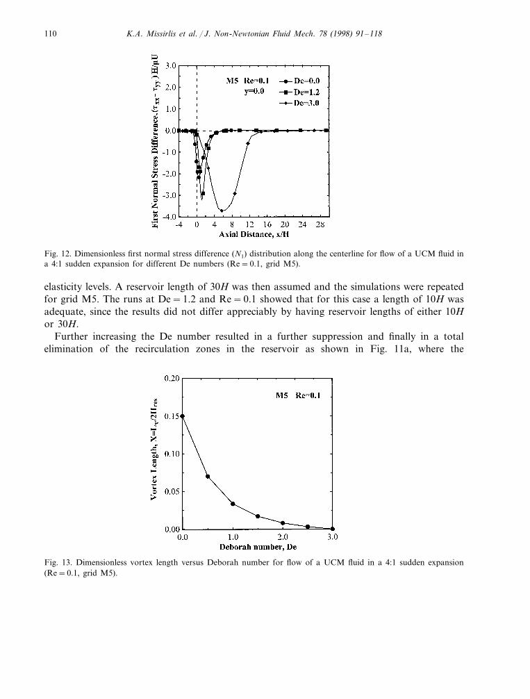
Fig. 12. Dimensionless first normal stress difference (N1) distribution along the centerline for flow of a UCM fluid ina 4:1 sudden expansion for different De numbers (Re=0.1, grid M5).

elasticity levels. A reservoir length of 30H was then assumed and the simulations were repeatedfor grid M5. The runs at De=1.2 and Re=0.1 showed that for this case a length of 10H wasadequate, since the results did not differ appreciably by having reservoir lengths of either 10Hor 30H.

Further increasing the De number resulted in a further suppression and finally in a totalelimination of the recirculation zones in the reservoir as shown in Fig. 11a, where the

Fig. 13. Dimensionless vortex length versus Deborah number for flow of a UCM fluid in a 4:1 sudden expansion(Re=0.1, grid M5).

K.A. Missirlis et al. / J. Non-Newtonian Fluid Mech. 78 (1998) 91–118 111

streamlines are presented for De=3.0 and Re=0.1. A bending of the streamlines is noticedtowards the walls as the fluid enters the sudden expansion. The pressure contours (Fig. 11b)along the channel are vertical only at the inlet and they are stretched deeply into the expansionreservoir. The maxima and minima are also much higher. The same type of behaviour isobserved for the normal and shear stresses as presented in Fig. 11c–e. This happens because theelastic behaviour of the fluid is much stronger than the viscous one.

The values of normal stresses provide useful information on the fluid behaviour in processingand their first difference N1=txx−tyy can be measured experimentally. Fig. 12 provides thedistribution of the dimensionless first normal stress difference N1 along the centerline for threevalues of the Deborah number. It is seen that it is zero in the inlet channel, goes through a highincrease after the entry in the expansion and then returns to zero farther and farther away as theelasticity level increases. This figure also shows how the maxima get transported down thechannel and that a sufficiently long domain is necessary for the stresses to fully relax back tozero.

Another feature of the problem at hand is the dimensionless vortex length X defined as [1,2]

X=Lv

2Hres, (35)

where Lv is the length of the vortex and 2Hres is the reservoir height (Fig. 1). Fig. 13 presentsX as a function of Deborah number. The dimensionless vortex length becomes reduced from itsNewtonian value of 0.15 down to 0.0 at De=3.0. It is thus established that viscoelasticityreduces and finally eliminates the small Newtonian vortex in expansions for creeping flows(small Re numbers).

5. Concluding remarks

In this paper, the flow of a UCM model fluid through a 4:1 sudden planar expansion has beenstudied using a stable finite volume scheme. The choice of the problem was due to its earlierstudy by another research group [16] by the same method, thus allowing a direct comparison.The solution method succeeds in obtaining accurate values for all variables (including thestresses) at elasticity levels up to De=3.0 with a variety of grids to establish results independentof grid density.

Using the FVM, correctly balanced forces over each control volume are obtained. As a result,the stresses near the singularity yield finite forces on the corner boundary. In addition, thenon-staggered grid, where the same set of control volumes is used for all primitive variables,offers great geometrical simplicity, especially for posing the boundary conditions near thesingularity. To enhance the accuracy of the method, the boundary conditions were imposed viaquadratic polynomials. Accurate calculation of the primitive variables yielded accurate calcula-tion of their first gradients, which are dominant in the source terms of the momentum equations.The numerical stability of the method depended on the order of precision in the calculation ofsource terms.

The conservation equations of stresses were transformed using the elastic–viscous splitmethod introduced by Perera and Walters [7]. The convective terms for the stresses were

K.A. Missirlis et al. / J. Non-Newtonian Fluid Mech. 78 (1998) 91–118112

computed using a first-order upwind scheme, while for the velocities a hybrid scheme wasused. A new method to discretize the source term of the momentum equations was intro-duced and the obstacle of flow type change occurring at high De was overcome. For low Deand grid density, the solution was compared against other numerical results available in theliterature [16] and found to give smoother and physically more correct results. For high Devalues (De\2.0), it was found necessary to extend the domain appreciably in order to giveenough length for the high viscoelastic stresses to relax. For De\3.0, it was found that thestresses become exceedingly high, thus requiring a much longer domain, severe under-relax-ation and a very high computational time, while the velocity field remained uninteresting(lack of recirculation).

The present simulations reinforce the point made previously by the Phan-Thien/Tannergroup that the FVM can be used as a viable alternative for the solution of viscoelasticproblems. The results are accurate and offer an improvement over previous numerical solu-tions. Although the present study has been applied to a UCM fluid in a relatively simplegeometry, it can be further extended to other more realistic constitutive equations, such asthe Phan-Thien/Tanner or Giesekus–Leonov models, etc. and to other geometries encoun-tered in polymer processing.

Acknowledgements

Financial assistance from the Natural Sciences and Engineering Research Council (NSERC)of Canada and the Ontario Center for Materials Research (OCMR) for Professor E. Mit-soulis is gratefully acknowledged.

Appendix A. Momentum interpolation

The momentum interpolation technique is used to avoid uniform pressure field in a non-staggered grid. From the momentum equations (Eqs. (10) and (11)) and referring to Fig. 3,when solving for the velocity uP and subtracting from the source term the part whichcontains the pressure, i.e. b=bP−AP(Pe−Pw), we obtain1

uP=% au

nbPunbP

auP

+bu

P

auP

−Ax

P

auP

(Pe−Pw) (A1)

Similarly for the velocity uE :

uE=% au

nbEunbE

auE

+bu

E

auE

−Ax

E

auE

(Pee−Pe) (A2)

The velocity at the east surface of the cell with P as its center is:

1 The exponents represent the primitive variable.

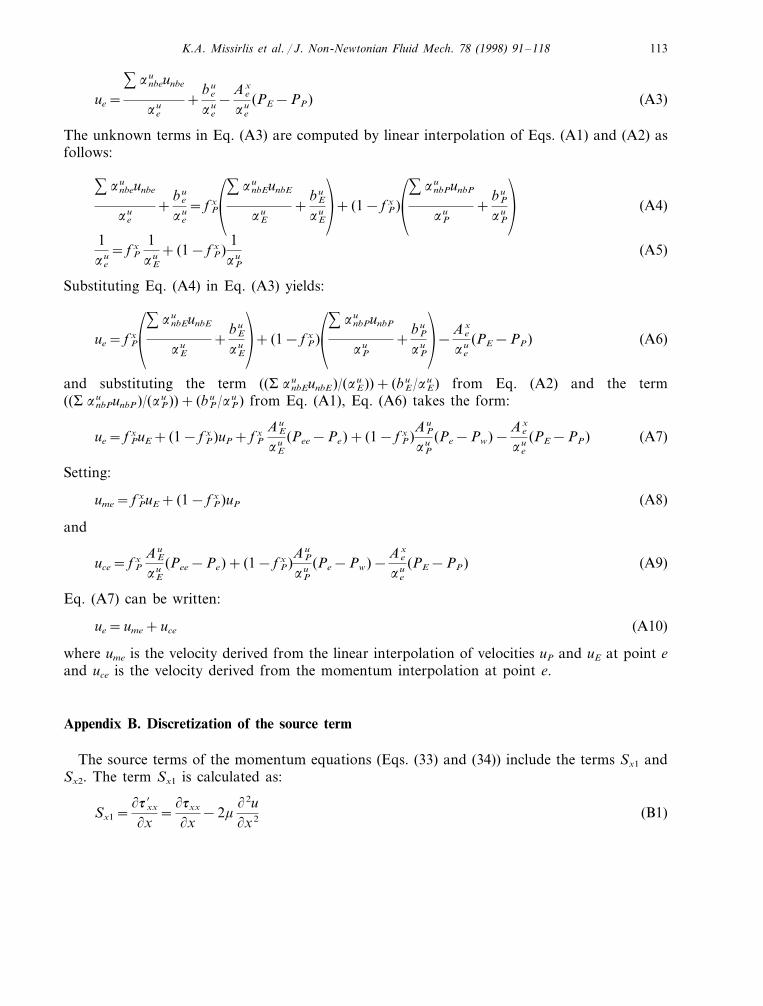
K.A. Missirlis et al. / J. Non-Newtonian Fluid Mech. 78 (1998) 91–118 113

ue=% au

nbeunbe

aue

+bu

e

aue

−Ax

e

aue

(PE−PP) (A3)

The unknown terms in Eq. (A3) are computed by linear interpolation of Eqs. (A1) and (A2) asfollows:

% aunbeunbe

aue

+bu

e

aue

= f xP

:% aunbEunbE

auE

+bu

E

auE

;+ (1− f x

P):% au

nbPunbP

auP

+bu

P

auP

;(A4)

1au

e

= f xP

1au

E

+ (1− f xP)

1au

P

(A5)

Substituting Eq. (A4) in Eq. (A3) yields:

ue= f xP

:% aunbEunbE

auE

+bu

E

auE

;+ (1− f x

P):% au

nbPunbP

auP

+bu

P

auP

;−

Axe

aue

(PE−PP) (A6)

and substituting the term ((� aunbEunbE)/(au

E))+ (buE/au

E) from Eq. (A2) and the term((� au

nbPunbP)/(auP))+ (bu

P/auP) from Eq. (A1), Eq. (A6) takes the form:

ue= f xPuE+ (1− f x

P)uP+ f xP

AuE

auE

(Pee−Pe)+ (1− f xP)

AuP

auP

(Pe−Pw)−Ax

e

aue

(PE−PP) (A7)

Setting:

ume= f xPuE+ (1− f x

P)uP (A8)

and

uce= f xP

AuE

auE

(Pee−Pe)+ (1− f xP)

AuP

auP

(Pe−Pw)−Ax

e

aue

(PE−PP) (A9)

Eq. (A7) can be written:

ue=ume+uce (A10)

where ume is the velocity derived from the linear interpolation of velocities uP and uE at point eand uce is the velocity derived from the momentum interpolation at point e.

Appendix B. Discretization of the source term

The source terms of the momentum equations (Eqs. (33) and (34)) include the terms Sx1 andSx2. The term Sx1 is calculated as:

Sx1=(t %xx

(x=(txx

(x−2m

(2u(x2 (B1)

K.A. Missirlis et al. / J. Non-Newtonian Fluid Mech. 78 (1998) 91–118114

The term (txx/(x is added in the source assuming quadratic variation of txx along thex-direction. Thus, (txx/(x is written as (2a1x+b1) Dx Dy. For the calculation of a1 and b1, thesame practice as that described in Appendix C was used, giving:

b1=txxP

−t %xxW

xP−xW

−a1(xP+xW) (B2)

a1=

txxE−txxW

xE−xW

−txxP

−txxW

xP−txxW

xE−xP

(B3)

The term −2m(((2u)/((x2)) is calculated by integrating it over the control volume V :&VP

−2m(2u(x2 dV=

& yn

y s

& xe

xw

−2m(2u(x2 dx dy= −2De(uE−uP)+2Dw(uP−uw) (B4)

Consequently:

Sx1= (2ax+b) Dx Dy−2De(uE−uP)+2Dw(uP−uw) (B5)

The term Sx2 is calculated as:

Sx2=(t %xy

(y=(txy

(y−m

(

(y�(u(y

+(6

(x�

(B6)

The term (txy/(y is calculated following the same method as in term Sx1. The term −m((/(y)(((u/(y)+ ((6/(x)) is calculated by integrating it over the control volume V :&

VP

−m(

(y�(u(y

+(6

(x�

dV=& yn

ys

& xe

xw

−m�(2u(y2+

(26

(y(x�

dx dy

= −Dn(uN−uP)+Ds(uP−uS)−m(6ne−6nw−6se+6sw) (B7)

Consequently:

Sx2= (2a2y+b2) Dx Dy−Dn(uN−uP)+Ds(uP−uS)−m(6ne−6nw−6se+6sw) (B8)

where:

b2=txyP

−txyS

yP−yS

−a2(yP+yS) (B9)

a2=

txyN−txyS

yN−yS

−txyP

−txyS

yP−yS

yN−yP

(B10)

The term Sy1 is calculated as:

Sy1=(t %yy

(y=(tyy

(y−2m

(26

(y2 (B11)

The term (tyy/(y is calculated following the same method as the derivative of stress in term Sx1.The term −2m((26/(y2) is calculated by integrating it over the control volume V :

K.A. Missirlis et al. / J. Non-Newtonian Fluid Mech. 78 (1998) 91–118 115

&VP

−2m(26

(y2 dV=& yn

yz

& xe

xw

−2m(26

(y2 dx dy= −2Dn(6N−6P)+2Ds(6P−6S) (B12)

Consequently:

Sy1= (2a3y+b3) Dx Dy−2Dn(6N−6P)+2Ds(6P−6S) (B13)

where:

b3=tyyP

−tyyS

yP−yS

−a3(yP+yS) (B14)

a3=

tyyN−tyyS

yN−yS

−tyyP

−tyyS

yP−yS

yN−yP

(B15)

The term Sy2 is calculated as:

Sy2=(t %xy

(x=(txy

(x−m

(

(x�(u(y

+(6

(x�

(B16)

The term (txy/(x is calculated following the same method as the derivative of stress in term Sx1.The term −m((/(x(((u/(y)+ ((6/(x)) is calculated by integrating it over the control volume V :&

VP

−m(

(x�(u(y

+(6

(x�

dV=& yn

ys

& xe

xw

−m(

(x�(u(y

+(6

(x�

dx dy (B17)

= −m(−une+use−unw+usw)−De(6E−6P)+Dw(6P−6W) (B18)

Consequently:

Sy2= (2a4x+b4) Dx Dy−m(−une+use−unw+usw)−De(6E−6P)+Dw(6P−6W) (B19)

where:

b4=txyP

−txyW

xP−xW

−a4(xP+xW) (B20)

a4=

txyE−txyW

xE−xW

−txyP

−txyW

xP−xW

xE−xP

(B21)

The terms Sx3 and Sy3 are discretized as follows:&VP

Sx3 dV=UL& xe

xw

& yn

ys

m(

(x�(u(x

+(6

(y�

dy dx (B22)

&VP

Sy3 dV=UL& yn

ys

& xe

xw

m(

(y�(u(x

+(6

(y�

dy dx (B23)

In the source term of the x-momentum equation the terms of Eq. (23) Sx5 is included adding inSC the term:

K.A. Missirlis et al. / J. Non-Newtonian Fluid Mech. 78 (1998) 91–118116

SC,x=UL� mAe

(dx)e

uE+mAw

(dx)w

uW+m(6en−6wn)−m(6es−6ws)n

(B24)

and in SP :

SP,x= −UL� mAe

(dx)e

+mAw

(dx)w

�(B25)

while in the source term of the y-momentum equation the terms of Eq. (23) Sy5 is includedadding in SC :

SC,y=UL� mAn

(dy)n

uN+mAs

(dy)s

us+m(uen−ues)−m(uwn−uws)n

(B26)

and in SP :

SP,y= −UL� mAn

(dy)n

+mAs

(dy)s

�(B27)

Appendix C. Neumann boundary conditions

The discretization of velocity gradients on the wall boundaries affects dramatically theaccuracy of the numerical method. A method to obtain second-order accuracy for the primitivevariables is to use quadratic polynomials for posing the boundary conditions on the wall [27],adapted for a non-uniform grid.

The wall force is entered into the discretized u-momentum equation as a source. The wallshear stress value is obtained from

tw=m(u(y)P

(C1)

The shear force Fs is now given by:

FS= −twA (C2)

where A is the wall area of the control volume.The appropriate source term in the u-equation is defined by:

S=mA�(u(y�)

wall(C3)

The computation of the u-gradient in the y-direction in Eq. (C3) is carried out assuming that uis a quadratic function of y :

u=ay2+by+g (C4)

giving:

(u(y

=2ay+b (C5)

K.A. Missirlis et al. / J. Non-Newtonian Fluid Mech. 78 (1998) 91–118 117

Applying Eq. (C3) to grid points N, P and S, the following equations are derived:

uN=ay2N+byN+g (C6)

uP=ay2P+byP+g (C7)

uS=ay2S+byS+g (C8)

In the above system of equations:

b=uP−uS

yP−yS

−a(yP+yS) (C9)

a=

uN−uS

yN−yS

−uP−uS

yP−yS

yN−yP

(C10)

Substituting Eq. (C5) in Eq. (C3) the following equation is valid:

S=mA(2ay �wall+b) (C11)

Finally the source term is obtained by substituting the values of a and b in Eq. (C11):

S=m

V

:2

uN−uS

yN−yS

−uP−uS

yP−yS

yN−yP

yN+uP−uS

yP−yS

−

uN−uS

yN−yS

−uP−uS

yP−yS

yN−yP

(yP+yS);Dx (C12)

References

[1] R. Keunings, Simulation of viscoelastic fluid flow, in: C.L. Tucker III (Ed.), Fundamentals of ComputerModelling for Polymer Processing, Carl Hanser Verlag, New York, 1989, pp. 403–469.

[2] E. Mitsoulis, Numerical simulation of viscoelastic fluids, in: N.P. Cheremisinoff (Ed.), Encyclopedia of FluidMechanics, vol. 9, Polymer Flow Engineering, Gulf Publishing Company, Dallas, Texas, USA, 1990, pp.649–704.

[3] R.I. Tanner, From A to (BK)Z in constitutive equations, J. Rheol. 32 (1988) 673–702.[4] H.P.W. Baaijens, G.W.M. Peters, F.P.T. Baaijens, H.E.H. Meijer, Viscoelastic flow past a confined cylinder of

a polyisobutylene solution, J. Rheol. 39 (1995) 1243–1277.[5] G. Barakos, E. Mitsoulis, Numerical simulation of viscoelastic flow around a cylinder using an integral

constitutive equation, J. Rheol. 39 (1995) 1279–1292.[6] M.J. Crochet, G. Pilate, Plane flow of a fluid of second grade through a contraction, J. Non-Newton. Fluid

Mech. 1 (1976) 247–258.[7] M.G.N. Perera, K. Walters, Long-range memory effects in flows involving abrupt changes in geometry. Part I.

Flows associated with L-shaped and T-shaped geometries, J. Non-Newton. Fluid Mech. 2 (1977) 49–81.[8] M.G.N. Perera, K. Walters, Long-range memory effects in flows involving abrupt changes in geometry. Part II.

The expansion-contraction-expansion problem, J. Non-Newton. Fluid Mech. 2 (1977) 191–204.[9] M.J. Crochet, A.R. Davies, K. Walters, Numerical Simulation of Non-Newtonian Flow, Elsevier, Amsterdam,

1984.[10] M.B. Bush, J.F. Milthorpe, R.I. Tanner, Finite element and boundary element methods for extrusion computa-

tions, J. Non-Newton. Fluid Mech. 16 (1984) 37–51.[11] M.B. Bush, R.I. Tanner, N. Phan-Thien, A boundary element investigation of extrudate swell, J. Non-Newton.

Fluid Mech. 18 (1985) 143–162.

K.A. Missirlis et al. / J. Non-Newtonian Fluid Mech. 78 (1998) 91–118118

[12] A.N. Beris, R.C. Armstrong, R.A. Brown, Spectral/finite element calculations of the flow of a Maxwell fluidbetween eccentric rotating cylinders, J. Non-Newton. Fluid Mech. 22 (1987) 129–167.

[13] S.V. Patankar, Numerical Heat Transfer and Fluid Flow, Hemisphere, New York, 1980.[14] H.H. Hu, D.D. Joseph, Numerical simulation of viscoelastic flow past a cylinder, J. Non-Newton. Fluid Mech.

37 (1990) 347–377.[15] J.Y. Yoo, Y. Na, A numerical study of the planar contraction flow of a viscoelastic fluid using SIMPLER

algorithm, J. Non-Newton. Fluid Mech. 39 (1991) 89–106.[16] M.S. Darwish, J.R. Whiteman, M.J. Bevis, Numerical modelling of viscoelastic liquids using a finite-volume

method, J. Non-Newton. Fluid Mech. 45 (1992) 311–337.[17] G.P. Sasmal, A finite volume approach for calculation of viscoelastic flow through an abrupt axisymmetric

contraction, J. Non-Newton. Fluid Mech. 47 (1995) 15–47.[18] R.I. Tanner, N. Phan-Thien, X. Huang, Two and three-dimensional finite volume methods for flows of

viscoelastic fluids, Proc. 4th Eur. Cong. Rheology, Seville, Spain, 1994, pp. 362–364.[19] S.C. Xue, N. Phan-Thien, R.I. Tanner, Numerical study of secondary flows of viscoelastic fluid in straight pipes

by an implicit finite volume method, J. Non-Newton. Fluid Mech. 59 (1995) 191–213.[20] X. Huang, N. Phan-Thien, R.I. Tanner, Viscoelastic flow between eccentric rotating cylinders: unstructured

control volume method, J. Non-Newton. Fluid Mech. 64 (1996) 71–92.[21] X.-L. Luo, A control volume approach for integral viscoelastic models and its application to contraction flow of

polymer melts, J. Non-Newton. Fluid Mech. 64 (1996) 173–189.[22] R.I. Tanner, Engineering Rheology, Clarendon Press, Oxford, 1985.[23] T.F. Miller, F.W. Schmidt, Use of a pressure weighted interpolation method for the solution of the incompress-

ible Navier–Stokes equations on a non-staggered grid system, Numer. Heat Transf. 14 (1988) 213–233.[24] S. Majumdar, Role of under-relaxation in momentum interpolation for calculation of flow with non-staggered

grids, Numer. Heat Transf. 13 (1988) 125–132.[25] J.P. Van Doormal, G.D. Raithby, Enhancement of the SIMPLE method for predicting incompressible flows,

Numer. Heat Transf. 7 (1984) 147–163.[26] C.R. Maliska, G.D. Raithby, Calculating 3D fluid flows using orthogonal grids, Proc. 3rd Int. Conf. Numerical

Methods in Laminar and Turbulent Flows, Seattle, WA, 1986, pp. 656–666.[27] D.A. Anderson, J.C. Tannehill, R.H. Pletcher, Computational Fluid Mechanics and Heat Transfer, McGraw-

Hill, New York, 1984, pp. 57–61.[28] C.A. Fletcher, Computational Techniques for Fluid Dynamics, vol. 2, 2nd ed., Springer, Berlin, 1991.[29] A.S. Mujumdar, R.A. Mashelkar, Advances in Transport Processes, vol. 3, Wiley, Chichester, 1984.[30] K. Missirlis, FIVOS: A FInite VOlume Solver for non-Newtonian flows, Internal Report, Department of

Chemical Engineering, NTUA, Athens, Greece, 1996.[31] L.H. Back, E.J. Roschke, Shear-layer flow regimes and wave instabilities and reattachment lengths downstream

of an abrupt circular channel expansion, J. Appl. Mech. 9 (1972) 677–681.[32] R.B. Bird, R.C. Armstrong, O. Hassager, Dynamics of Polymeric Liquids, vol. 1, Fluid Mechanics, Wiley, New

York, 1977.

.