A FAST UNIVERSAL SOLVER FOR 1D CONTINUOUS AND DISCONTINUOUS STEADY FLOWS IN RIVERS AND PIPES

François Kerger

Belgian National Fund for Scientific Research F.R.S - FNRS

Research unit of Hydrology, Applied Hydrodynamics and Hydraulic Constructions (HACH),

ArGEnCo Department – MS²F – University of Liege (ULg)

Chemin des Chevreuils, 1 B52/3 B-4000 Liege, Belgium

e-mail: fkerger@ulg.ac.be

tel: 00 32 4 366 90 04

fax : 00 32 4 366 95 58

Pierre Archambeau

Research unit of Hydrology, Applied Hydrodynamics and Hydraulic Constructions (HACH),

ArGEnCo Department – MS²F – University of Liege (ULg)

Chemin des Chevreuils, 1 B52/3 B-4000 Liege, Belgium

Sébastien Erpicum

Research unit of Hydrology, Applied Hydrodynamics and Hydraulic Constructions (HACH),

ArGEnCo Department – MS²F – University of Liege (ULg)

Chemin des Chevreuils, 1 B52/3 B-4000 Liege, Belgium

Benjamin Dewals

Belgian National Fund for Scientific Research F.R.S - FNRS

Research unit of Hydrology, Applied Hydrodynamics and Hydraulic Constructions (HACH),

ArGEnCo Department – MS²F – University of Liege (ULg)

Chemin des Chevreuils, 1 B52/3 B-4000 Liege, Belgium

Michel Pirotton

Research unit of Hydrology, Applied Hydrodynamics and Hydraulic Constructions (HACH),

ArGEnCo Department – MS²F – University of Liege (ULg)

Chemin des Chevreuils, 1 B52/3 B-4000 Liege, Belgium

1. Introduction One dimensional numerical simulation of free-surface and pressurized flows is a useful engineering tool for a wide range of practical applications in civil engineering. The method can be used as long as no 2D and 3D hydraulic effects are predominant and must be thus taken into account. For instance, large rivers networks are often managed and developed by means of 1D models [1, 2]. Similarly, simulation of pressurized flow in pipes networks such as water supply or sewer systems relies traditionally on such models [3, 4]. Finally, 1D models can be reliably considered in the design process of many hydraulic structures such as water intake, bottom outlet tailrace tunnel, flushing galleries in dams [5]. On account of the large number of practical applications concerned, an efficient prediction of 1D flow features is an obvious need. Developing a unified 1D model for all the situations of interest in civil engineering remains however challenging. Various flow patterns may indeed coexist in actual situations:

1. Free surface flows, where supercritical, subcritical and transcritical conditions could co-exist [2], are usually modelled, including the discontinuities (hydraulic jump), on the basis of the conservative Saint-Venant equations [6, 7].

2. Pressurized flows are traditionally described by the water hammer equations [4]. 3. Mixed flows, characterized by a simultaneous occurrence of free-surface and

pressurized flow, are still nowadays an issue of research [8-11] for its mathematical description and its numerical solution.

To achieve our purpose to develop a universal solver handling free-surface, pressurized and mixed flow, it is then required

1. to establish a unified mathematical model which overcomes the dissimilarity between the sets of equations describing pressurized and free-surface flows;

2. to set an efficient resolution scheme for this model. As previously mentioned, different mathematical approaches to describe free-surface, pressurized and mixed flow in a unified framework have been developed to date and are still subject to many research. Shock-tracking methods consists in solving separately free-surface and pressurized flows through different sets of equations [12, 13]. Rigid Water Column Approach treats each phase separately on the basis of a specific set of equations in focusing on the air behaviour [14]. Nevertheless, such algorithms are very complicated and case-specific. Finally, the so-called shock-capturing approach is a family of method which computes pressurized and free-surface flows by using a single set of equations [8-11] . In this paper, such an approach is used, based on the model of the Preissmann slot [15]. In particular, this paper focuses on steady state flows which are of great interest for engineers. Design guidelines for many hydraulic structures specify indeed that specific critical steady states have to be addressed. Practitioners should then rely on robust and efficient 1D solvers suitable for each flow pattern (free-surface, pressurized and mixed) in order to evaluate situations in rivers, pipes and all the common hydraulic structures. Traditionally, computation of such steady states is performed with traditional methods for solving ordinary differential equation [16], which require setting apart supercritical and subcritical flows and treat regime transitions in a particular way (see section 2.2 for further details). These two features are their major drawback. Another method consists in discretizing the unsteady mathematical model by means of a shock-capturing finite volume method [17] and in computing the scheme over a sufficient number of time steps in order to converge on the steady state solution. Since a system of Partial Differential Equations (PDE’s) is solved instead of an ordinary differential equation, this method requires a pointless computational effort. In this paper, a fast universal solver for 1D continuous and discontinuous steady flows in rivers and pipes is set up and assessed. Developments are initiated from an original unified mathematical model using the Saint-Venant equations and the Preissmann slot model. The

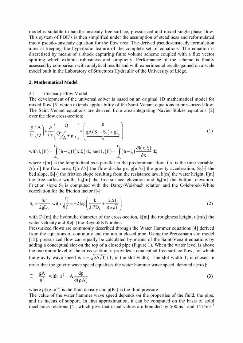
model is suitable to handle unsteady free-surface, pressurized and mixed single-phase flow. This system of PDE’s is then simplified under the assumption of steadiness and reformulated into a pseudo-unsteady equation for the flow area. The derived pseudo-unsteady formulation aims at keeping the hyperbolic feature of the complete set of equations. The equation is discretised by means of a shock capturing finite volume scheme coupled with a flux vector splitting which exhibits robustness and simplicity. Performance of the scheme is finally assessed by comparison with analytical results and with experimental results gained on a scale model built in the Laboratory of Structures Hydraulic of the University of Liège. 2. Mathematical Model 2.1 Unsteady Flow Model The development of the universal solver is based on an original 1D mathematical model for mixed flow [5] which extends applicability of the Saint-Venant equations to pressurized flow. The Saint-Venant equations are derived from area-integrating Navier-Stokes equations [2] over the flow cross-section:

( )20 f 2

1S

0QAgA S S gIQQt x gIA

⎛ ⎞⎛ ⎞⎛ ⎞∂ ∂ ⎜ ⎟⎜ ⎟+ = − +⎜ ⎟ ⎜ ⎟∂ ∂ ⎜ ⎟+⎝ ⎠ ⎝ ⎠ ⎝ ⎠

(1)

with ( ) ( ) ( ) ( ) ( ) ( )fs fs

b b

h h

1 2h h

l x,I h h l x, d and I h h d

x− −

∂ ξ= − ξ ξ ξ = − ξ ξ

∂∫ ∫

where x[m] is the longitudinal axis parallel to the predominant flow, t[s] is the time variable, A[m²] the flow area, Q[m³/s] the flow discharge, g[m²/s] the gravity acceleration, S0[-] the bed slope, Sf[-] the friction slope resulting from the resistance law, h[m] the water height, l[m] the free-surface width, hfs[m] the free-surface elevation and hb[m] the bottom elevation. Friction slope Sf is computed with the Darcy-Weisbach relation and the Colebrook-White correlation for the friction factor f[-]:

2

fh h

fu 1 k 2.51S with 2log 2gD f 3.7D Re f

⎛ ⎞= = − +⎜ ⎟

⎝ ⎠ (2)

with Dh[m] the hydraulic diameter of the cross-section, k[m] the roughness height, u[m/s] the water velocity and Re[-] the Reynolds Number. Pressurized flows are commonly described through the Water Hammer equations [4] derived from the equations of continuity and motion in closed pipe. Using the Preissmann slot model [15], pressurized flow can equally be calculated by means of the Saint-Venant equations by adding a conceptual slot on the top of a closed pipe (Figure 1). When the water level is above the maximum level of the cross-section, it provides a conceptual free surface flow, for which the gravity wave speed is sc gA T= (Ts is the slot width). The slot width Ts is chosen in order that the gravity wave speed equalizes the water hammer wave speed, denoted a[m/s]:

( )2

s 2

gA dpT with a Aa d A

= =ρ

(3)

where ρ[kg.m-3] is the fluid density and p[Pa] is the fluid pressure. The value of the water hammer wave speed depends on the properties of the fluid, the pipe, and its means of support. In first approximation, it can be computed on the basis of solid mechanics relations [4], which give that usual values are bounded by 500ms-1 and 1414ms-1

(for an infinitely rigid pipe). Physically, the slot accounts for the water compressibility and the pipe dilatation under a variation of pressure. Usual width for the Preissmann slot is computed between by 10-4m and 10-9m. From a hydraulic point of view, all the relevant information is summarized in relations water height/flow area (H-A). A specific relation corresponds to each geometry of the cross-section (figure 1a). Adding the Preissmann slot leads to linearly extend the relation beyond the pipe crown head (figure 1b). In order to simulate pressurized flows with a piezometric head below the top of the pipe section, an original concept, called negative Preissmann slot, has been developed. It consists in extending the Preissmann straight line for water height below the pipe crown (figure 1c). To each water height below the pipe crown correspond two values of the flow area: one for the free surface flow and one corresponding to the pressurized flow. One of them is chosen depending on the local aeration conditions (closed pipe or presence of an air vent). For further details, we refer the interested reader to the following papers [5, 18] totally dedicated to this mathematical model. The study of the characteristic velocities λ1 and λ2 of the system (1) leads to the following values depending only on the fluid velocities u[m/s] and the gravity wave speed c[m/s] given above:

( )( )

1

2

u c c Fr 1

u c c Fr 1

λ = − = −⎧⎪⎨λ = + = +⎪⎩

(4)

where Fr[-] is the Froude number [2]. Examining the sign of the expression (4) shows that a supercritical flow (|Fr| > 1) requires two upstream boundary conditions. In a similar manner, it is proved that subcritical flow (|Fr| < 1) requires both an upstream and downstream boundary conditions. 2.2 Steady Flow Model The ordinary differential equation for steady flow may be obtained from the system of PDE’s given by equation (1). By assuming that each time derivative is equal to zero (∂A/∂t=∂Q/∂t=0), equation (1) is written as follows:

st

2

1

Q Cd Q gI SAdx

⎧ =⎪⎨ ⎛ ⎞+ =⎜ ⎟⎪ ⎝ ⎠⎩

(5)

where integrals I1 and I2 are defined as above and the friction slope is computed on the basis of equation (2). First equation in (5) is trivial since the discharge is imposed by boundary conditions upstream the computational domain. In order to solve unique unknown A, several numerical techniques can be applied. As mentioned in the introduction, equation (5) is traditionally simplified by using standard properties of the derivatives as an ordinary differential equation (ODE):

( )2

22

S AdAQdx a A

=−

(6)

where the celerity is given by equation (3). In principle, standard methods could solve this ODE but the presence of a singularity for trans-critical flow in which Q/A ≅ a make this methods fail. Specific methods derived for the purpose of solving equation (6) require to set apart supercritical and subcritical flows and to treat the singularity (regime transitions) with caution.

The original method presented in this paper consists in deriving a pseudo-unsteady equation to solve steady flow instead of using the actual unsteady system of PDE’s (1) or the simplified ODE (6). A pseudo-unsteady strategy enables to keep the hyperbolic feature of the equation and to apply the same resolution schemes as those used traditionally for the Saint-Venant equations. The pseudo-unsteady strategy consists in adding a pseudo-temporal term into the ordinary differential equation (5), denoted τ to avoid confusion with the full unsteady model. The introduction of the new term provides however an additional degree of freedom (parameter β) that must be determined subsequently:

2

1A Q gI SAx∂ ∂ ⎛ ⎞β + + =⎜ ⎟∂τ ∂ ⎝ ⎠

(7)

In this model, the flow discharge is now a given parameter of the problem. The characteristic velocity λ is given by:

( )2 22 2 c 1 Frc u −−λ = =

β β (8)

The sign of the real characteristic velocity only depends on the value of the degree of freedom β and the flow regime. Table 1 shows that a supercritical flow (|Fr| > 1) requires only an upstream boundary condition if β is negative and only a downstream boundary condition if β is positive. The exact opposite conclusion holds for a subcritical flow (|Fr| < 1). Comparing the sign of λ with the sign of the characteristics velocities λ1 and λ2 introduced in equation (4) gives an insight into the value of β to select. Indeed, it has been shown that the system of equations (1) for unsteady flow requires two upstream boundary conditions for a supercritical flow. As the discharge is assumed constant, the pseudo-steady model (7) would require only one upstream boundary condition for a supercritical flow if β is chosen as negative. In conclusion, β is imposed as negative in order to keep the new model consistent with the full unsteady model. What is more, the value of β does not affect the rate of convergence of the scheme such that it can be simply set to ( )sign Qβ = − . 2.3 Numerical Model Both the unsteady and the pseudo-unsteady models have been implemented in the modelling system WOLF [19, 20] which has been developed in the last ten years within the Research Unit of Hydrology, Applied Hydrodynamics and Hydraulic Constructions of the University of Liège. Discretization of equation (7) is performed by means of a finite volume scheme over uniform grid cells of length 1 1

2 2k kx x x ,k 1...N+ −Δ = − = (Figure 2):

1 12 2

n nk k n

kk

F FA Sx

+ −−∂⎛ ⎞β + =⎜ ⎟∂τ Δ⎝ ⎠ (9)

where n is the time index and the numerical flux 12

nkF + is computed with an original flux

vector splitting [21, 22]:

( )12

2nn

1k n k 1k

QF gIA+ +

= + (10)

It results in an explicit scheme in a conservation form which is shown hereafter unconditionally stable.

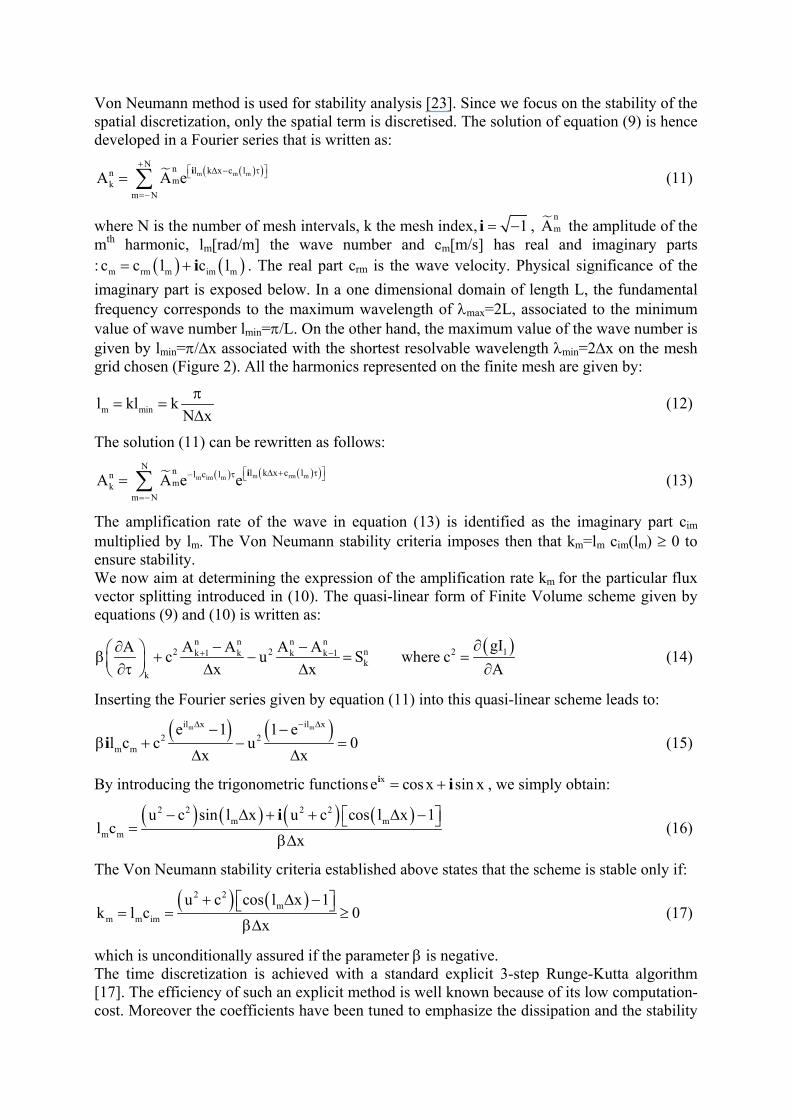
Von Neumann method is used for stability analysis [23]. Since we focus on the stability of the spatial discretization, only the spatial term is discretised. The solution of equation (9) is hence developed in a Fourier series that is written as:

( )( )m m mN n l k x c ln

mkm N

A A e+

⎡ ⎤Δ − τ⎣ ⎦

=−

= ∑ i (11)

where N is the number of mesh intervals, k the mesh index, 1= −i , nmA the amplitude of the

mth harmonic, lm[rad/m] the wave number and cm[m/s] has real and imaginary parts : ( ) ( )m rm m im mc c l c l= + i . The real part crm is the wave velocity. Physical significance of the imaginary part is exposed below. In a one dimensional domain of length L, the fundamental frequency corresponds to the maximum wavelength of λmax=2L, associated to the minimum value of wave number lmin=π/L. On the other hand, the maximum value of the wave number is given by lmin=π/Δx associated with the shortest resolvable wavelength λmin=2Δx on the mesh grid chosen (Figure 2). All the harmonics represented on the finite mesh are given by:

m minl kl kN xπ

= =Δ

(12)

The solution (11) can be rewritten as follows:

( ) ( )( )m rm mm im mN n l k x c ll c ln

mkm N

A A e e⎡ ⎤Δ + τ− τ ⎣ ⎦

=−

= ∑ i (13)

The amplification rate of the wave in equation (13) is identified as the imaginary part cim multiplied by lm. The Von Neumann stability criteria imposes then that km=lm cim(lm) ≥ 0 to ensure stability. We now aim at determining the expression of the amplification rate km for the particular flux vector splitting introduced in (10). The quasi-linear form of Finite Volume scheme given by equations (9) and (10) is written as:

( )n n n n2 2 n 2 1k 1 k k k 1

kk

gIA A A A Ac u S where cx x A

+ − ∂∂ − −⎛ ⎞β + − = =⎜ ⎟∂τ Δ Δ ∂⎝ ⎠ (14)

Inserting the Fourier series given by equation (11) into this quasi-linear scheme leads to:

( ) ( )m mil x il x2 2

m m

e 1 1 el c c u 0

x x

Δ − Δ− −β + − =

Δ Δi (15)

By introducing the trigonometric functions xe cos x sin x= +i i , we simply obtain:

( ) ( ) ( ) ( )2 2 2 2m m

m m

u c sin l x u c cos l x 1l c

x− Δ + + Δ −⎡ ⎤⎣ ⎦=

βΔ

i (16)

The Von Neumann stability criteria established above states that the scheme is stable only if:

( ) ( )2 2m

m m im

u c cos l x 1k l c 0

x+ Δ −⎡ ⎤⎣ ⎦= = ≥

βΔ (17)

which is unconditionally assured if the parameter β is negative. The time discretization is achieved with a standard explicit 3-step Runge-Kutta algorithm [17]. The efficiency of such an explicit method is well known because of its low computation-cost. Moreover the coefficients have been tuned to emphasize the dissipation and the stability

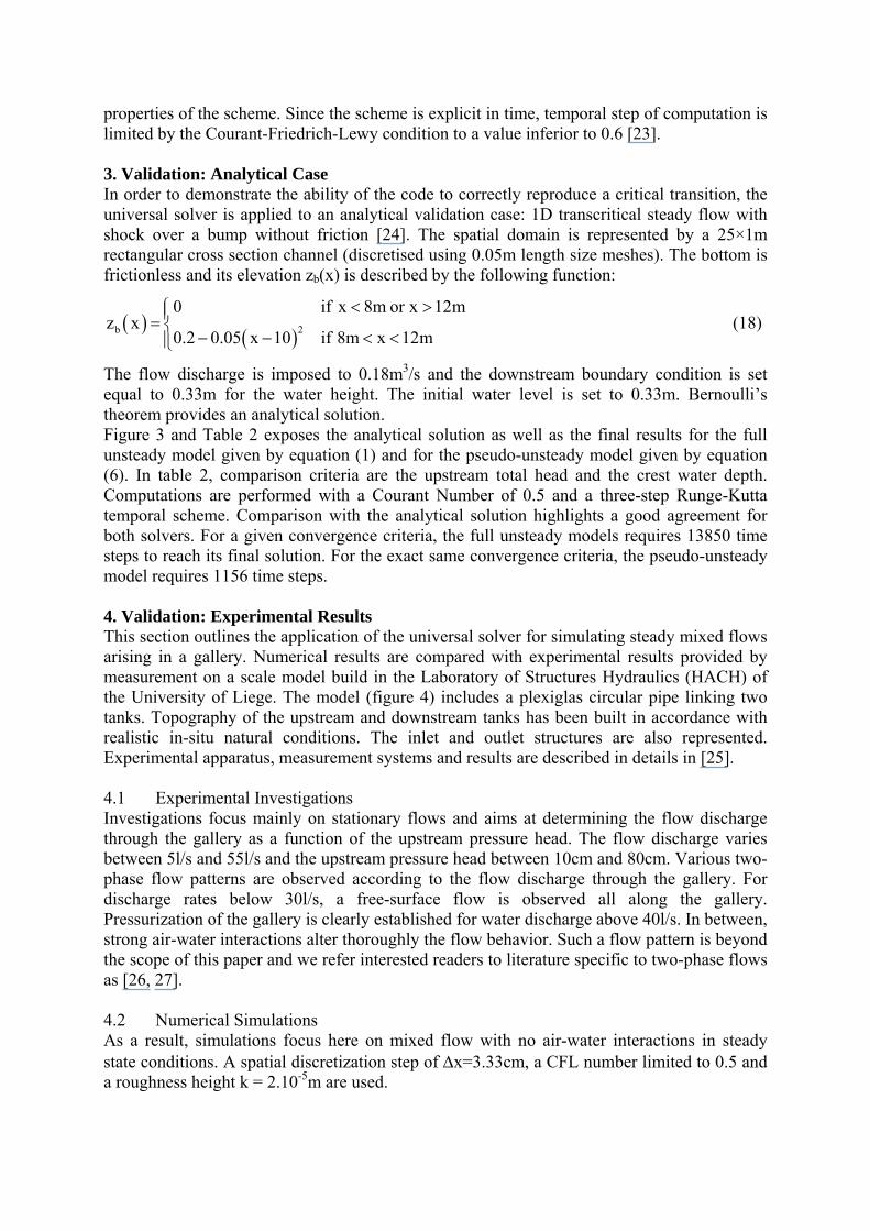
properties of the scheme. Since the scheme is explicit in time, temporal step of computation is limited by the Courant-Friedrich-Lewy condition to a value inferior to 0.6 [23]. 3. Validation: Analytical Case In order to demonstrate the ability of the code to correctly reproduce a critical transition, the universal solver is applied to an analytical validation case: 1D transcritical steady flow with shock over a bump without friction [24]. The spatial domain is represented by a 25×1m rectangular cross section channel (discretised using 0.05m length size meshes). The bottom is frictionless and its elevation zb(x) is described by the following function:

( )( )2b

0 if x 8m or x 12mz x

0.2 0.05 x 10 if 8m x 12m

< >⎧⎪= ⎨− − < <⎪⎩

(18)

The flow discharge is imposed to 0.18m3/s and the downstream boundary condition is set equal to 0.33m for the water height. The initial water level is set to 0.33m. Bernoulli’s theorem provides an analytical solution. Figure 3 and Table 2 exposes the analytical solution as well as the final results for the full unsteady model given by equation (1) and for the pseudo-unsteady model given by equation (6). In table 2, comparison criteria are the upstream total head and the crest water depth. Computations are performed with a Courant Number of 0.5 and a three-step Runge-Kutta temporal scheme. Comparison with the analytical solution highlights a good agreement for both solvers. For a given convergence criteria, the full unsteady models requires 13850 time steps to reach its final solution. For the exact same convergence criteria, the pseudo-unsteady model requires 1156 time steps. 4. Validation: Experimental Results This section outlines the application of the universal solver for simulating steady mixed flows arising in a gallery. Numerical results are compared with experimental results provided by measurement on a scale model build in the Laboratory of Structures Hydraulics (HACH) of the University of Liege. The model (figure 4) includes a plexiglas circular pipe linking two tanks. Topography of the upstream and downstream tanks has been built in accordance with realistic in-situ natural conditions. The inlet and outlet structures are also represented. Experimental apparatus, measurement systems and results are described in details in [25]. 4.1 Experimental Investigations Investigations focus mainly on stationary flows and aims at determining the flow discharge through the gallery as a function of the upstream pressure head. The flow discharge varies between 5l/s and 55l/s and the upstream pressure head between 10cm and 80cm. Various two-phase flow patterns are observed according to the flow discharge through the gallery. For discharge rates below 30l/s, a free-surface flow is observed all along the gallery. Pressurization of the gallery is clearly established for water discharge above 40l/s. In between, strong air-water interactions alter thoroughly the flow behavior. Such a flow pattern is beyond the scope of this paper and we refer interested readers to literature specific to two-phase flows as [26, 27]. 4.2 Numerical Simulations As a result, simulations focus here on mixed flow with no air-water interactions in steady state conditions. A spatial discretization step of Δx=3.33cm, a CFL number limited to 0.5 and a roughness height k = 2.10-5m are used.

Experimental and numerical data for the distribution of the total head and the pressure head (water level for free surface flow) along the gallery length are given in figure 5 for a free-surface flow (discharge of 9.5l/s) and a fully pressurized flow (discharge of 48.4l/s). In the latter case, results are in full agreement. The chart clearly shows the head loss at the gallery inlet is correctly simulated. In particular, a great variation in pressure at the entrance is accurately simulated with the numerical model. For the free-surface flow, a slight discrepancy is observed in the total head curve. It results from the effect of the air phase flowing above the free surface that is not taken into account in this computation. A comparison of the results given by the computation for a flow of 38.4l/s discharge is shown in figure 6. Pressure distribution along the gallery is computed in figure 6b under the assumption of a free surface flow appears if the pressure head is below the pipe crown. Large discrepancies of the results are observed. The upstream pressure head is overestimated. In figure 6a, activation of the negative Preissmann slot gives the curve corresponding to a pressurized flow. We consequently identify a large area of sub-atmospheric pressure in the upstream part of the pipe. Results are now in better accordance and lead to conclude that the aeration rate of the pipe is not sufficient to induce the apparition of a free surface flow. The necessity of the negative Preissmann is in this case obvious. 5. Conclusions In this paper, a single pseudo-unsteady equation is derived to describe in a unified framework all kinds of steady flow relevant in civil engineering. This pseudo unsteady model is simplified from a full unsteady model in a way that enables the new model to keep the hyperbolic feature of the full model. The mathematical model used as a basis for the original development is a system of PDE’s handling free-surface, pressurized and mixed flow in a unified framework. For this purpose, applicability of the Saint-Venant equations is extended to pressurized flow by means of the Preissmann slot model. The original point in this mathematical model is the concept of Negative Preissmann slot which enables to deal with sub-atmospheric pressurized flow. From a practical point of view, the pseudo-unsteady equation is implemented by means of a Finite-Volume scheme coupled with an original Flux-Vector Splitting (shock-capturing method), whose stability is demonstrated on the basis of the Von Neumann method. The pseudo-temporal path to evolve towards the final steady state proves to be efficient and robust. In particular, performance of the model is assessed by comparison with analytical and experimental results. The iterative method saves much computational time. The global performance can be improved further by means of a “local time stepping” strategy when the calculation domain involves pressurized meshes and free-surface meshes characterized by wide variations of the characteristic velocity. In addition, simulation of air-water interactions by means of a drift-flux model would widen the applicability of the solver to new applications. References

[1]. Goutal, N. and F. Maurel, A finite volume solver for 1D shallow-water equations applied to an actual river. International Journal for Numerical Methods in Fluids, 2002. 38(1): p. 1-19.

[2]. Cunge, J.A., F.M. Holly, and A. Verwey, Practical Aspects of Computational River Hydraulics. Monographs and surveys in water resources engineering. 1980, Boston: Pitman Advanced Pub. Program.

[3]. Leon, A.S., M.S. Ghidaoui, A.R. Schmidt, and M.H. Garcia, Efficient second-order accurate shock-capturing scheme for modeling one- and two-phase water hammer flows. Journal of Hydraulic Engineering, 2008. 134(7): p. 970-983.

[4]. Wylie, E.B. and V.L. Streeter, Fluid Transients. Première ed, ed. M.-H. Inc. 1978. 385.

[5]. Kerger, F., P. Archambeau, S. Erpicum, B.J. Dewals, and M. Pirotton, Simulation numérique des écoulements mixtes hautement transitoire dans les conduites d'évacuation des eaux. Houille Blanche-Rev. Int., 2009. 2009(5).

[6]. Cunge, J.A. and M. Wegner, Intégration numérique des équations d’écoulement de Barré de Saint Venant par un schéma implicite de différences finies. La Houille Blanche 1964: p. 33-39.

[7]. Aldrighetti, E. and P. Zanolli, A high resolution scheme for flows in open channels with arbitrary cross-section. International Journal for Numerical Methods in Fluids, 2005. 47(8-9): p. 817-824.

[8]. Bourdarias, C. and S. Gerbi, A Finite Volume Scheme for a Model Coupling Unsteady Flows in Open Channels and in Pipelines. Journal of Computational and Applied Mathematics, 2007. 209(1): p. 109-131.

[9]. Bourdarias, C., M. Ersoy, and S. Gerbi, A kinetic scheme for pressurized flows in non uniform closed water pipes. Monograf´ıas de la Real Academia de Ciencias de Zaragoza, 2009. 31: p. 1-20.

[10]. Vasconcelos, J., S. Wright, and P.L. Roe, Improved Simulation of Flow Regime Transition in Sewers : The Two-Component Pressure Approach. Journal of Hydraulic Engineering, 2006. 132(6): p. 553-562.

[11]. Trieu Dong, N., Numerical simulation of the flow in a conduit, in the presence of a confined air cushion. International Journal for Numerical Methods in Fluids, 1998. 29: p. 485-498.

[12]. Cardle, J. and C. Song, Mathematical Modeling of Unsteady Flow in Storm Sewers. International Journal of Engineering Fluid Mechanics, 1988. 1(4): p. 495-518.

[13]. Trajkovic, B., M. Ivetic, F. Calomino, and A. D'Ippolito, Investigation of Transition From Free Surface to Pressurized Flow in a Circular Pipe. Water Science and Technology, 1999. 39(9): p. 115-112.

[14]. Li, J. and A. McCorquodale, Modeling Mixed Flow in Storm Sewers. Journal of Hydraulic Engineering, 1999. 125(11): p. 1170-1180.

[15]. Preissmann, A. Propagation des intumescences dans les canaux et rivieres. in First Congress of the French Association for Computation. 1961. Grenoble, France.

[16]. Arbenz, K. and O. Bachmann, Eléments d'analyse numérique et appliquée. 1992: Presses Polytechniques et Universitaires Romandes (PPUR).

[17]. Leveque, R.J., Finite Volume Methods for Hyperbolic Problems. Cambridge texts in Applied Mathematics. 2002: Cambridge University Press. 540.

[18]. Kerger, F., S. Erpicum, P. Archambeau, B.J. Dewals, and M. Pirotton. Numerical Simulation of 1D Mixed Flow with Air/Water Interaction in Multiphase Flow V. 2009. New Forest, UK.

[19]. Erpicum, S., T. Meile, B.J. Dewals, M. Pirotton, and A. Schleiss, 2D numerical flow modeling in a macro-rough channel. International Journal for Numerical Methods in Fluids, 2009. published online.

[20]. Dewals, B.J., S. Erpicum, P. Archambeau, S. Detrembleur, and M. Pirotton, Depth-Integrated Flow Modelling Taking into Account Bottom Curvature. Journal of Hydraulic Research, 2006. 44(6): p. 787-795.

[21]. Dewals, B.J., S.A. Kantoush, S. Erpicum, M. Pirotton, and A. Schleiss, Experimental and numerical analysis of flow instabilities in rectangular shallow basins. Environmental Fluid Mechanics, 2008. 8(1): p. 31-54.

[22]. Erpicum, S., B.J. Dewals, P. Archambeau, and M. Pirotton, Dam-break flow computation based on an efficient flux-vector splitting. J. Comput. Appl. Math., 2009: p. accepted.

[23]. Hirsch, C., Numerical Computation of Internal and External Flows - Fundamentals of Numerical Discretization. Vol. 1. 1988, Chichester: Wiley. 515.

[24]. Caleffi, V., A. Valiani, and A. Zanni, Finite volume method for simulating extreme flood events in natural channels. Journal of Hydraulic Research, 2003. 41(2): p. 167-177.

[25]. Erpicum, S., F. Kerger, P. Archambeau, B.J. Dewals, and M. Pirotton. Experimental and numerical investigation of mixed flow in a Gallery. in Multiphase Flow V. 2009. New Forest: WIT Press.

[26]. Ishii, M. and T. Hibiki, Thermo-fluid dynamics of two-phase flow. First ed. 2006: Springer Science, USA. 430.

[27]. Kerger, F., B.J. Dewals, S. Erpicum, P. Archambeau, and M. Pirotton, An Extended Shallow-water-like Model Applied to Flows in Environmental and Civil Engineering, in Hydraulic Engineering: Structural Applications, Numerical Modeling and Environmental Impacts, G. Hirsch and B. Kappel, Editors. 2010, Nova Science Publishers: New-York. p. 1-70.

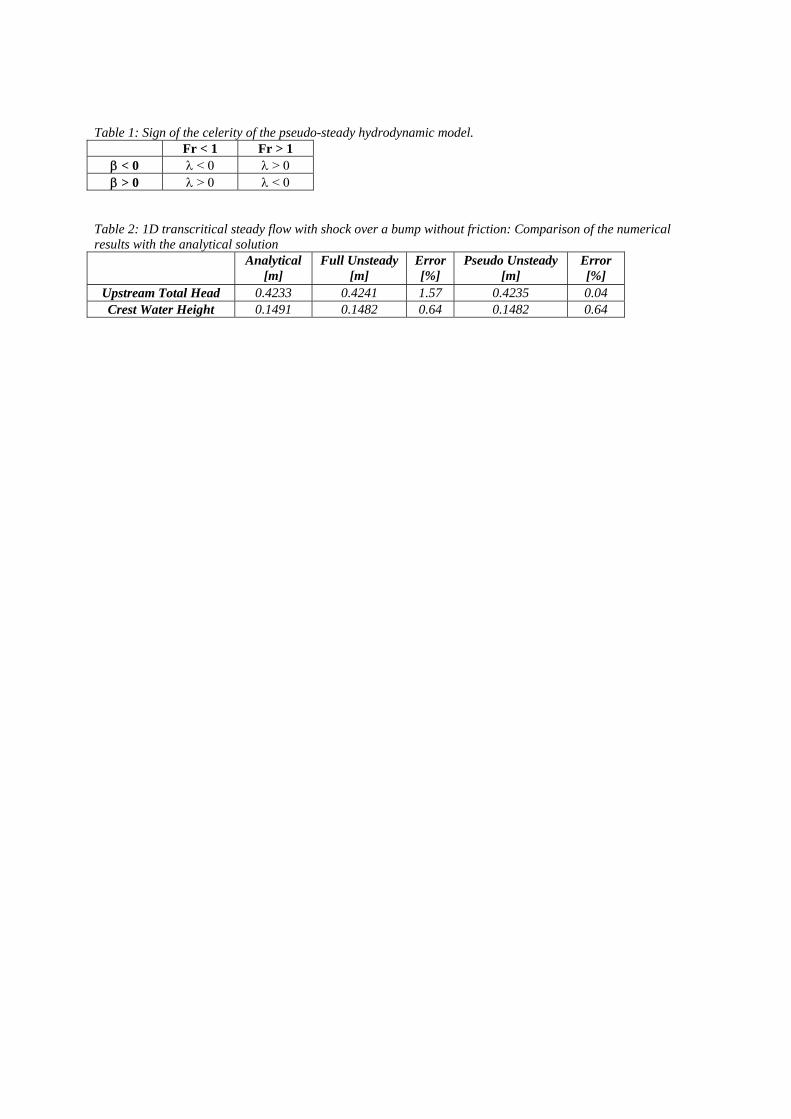
Table 1: Sign of the celerity of the pseudo-steady hydrodynamic model. Fr < 1 Fr > 1

β < 0 λ < 0 λ > 0 β > 0 λ > 0 λ < 0

Table 2: 1D transcritical steady flow with shock over a bump without friction: Comparison of the numerical results with the analytical solution

Analytical

[m] Full Unsteady

[m] Error [%]

Pseudo Unsteady [m]

Error [%]

Upstream Total Head 0.4233 0.4241 1.57 0.4235 0.04 Crest Water Height 0.1491 0.1482 0.64 0.1482 0.64