A Fast Distributed Algorithm for Mining Association Rules

A Fast Distributed Algorithm for Mining Association Rules *

David W. Cheungt Jiawei Hans Vincent T. Ngtt Ada W. Fuss Yongjian F u I

t Department of Computer Science, The University of Hong Kong, Hong Kong. Email: dcheungOcs.hku.hk. * School of Computing Science, Simon Fraser University, Canada. Email: hanOcs.sfu.ca.

tt Department of Computing, Hong Kong Polytechnic University, Hong Kong. Email: cstyngOcomp.po1yu.edu.hk.

$4 Department of Computer Science and Engineering, The Chinese University of Hong Kong,Hong Kong. Email: adafuOcs.cuhk.hk.

Abstract With the existence of many large transaction

databases, the huge amounts of data, the high scalability of distributed systems, and the easy partition and distribution of a centralized database, it is important to inuestzgate eficient methods for distributed mining of association rules. This study discloses some interesting relationships between locally large and globally large itemsets and proposes an interesting distributed association rule mining algorithm, FDM (Fast Distributed Mining of association rules), which generates a small number of candidate sets and substantially reduces the number of messages to be passed at mining association rules. Our performance study shows that FDM has a superior performance over the direct application of a typical sequential algorithm. Further performance enhancement leads to a few variations of the algorithm.

1 Introduction An association rule is a rule which implies certain

association relationships among a set of objects (such as “occur together” or “one implies the other”) in a database. Since finding interesting association rules in databases may disclose some useful patterns for decision support, selective marketing, financial fore- cast, medical diagnosis, and many other applications, it has attracted a lot of attention in recent data mining research [5]. Mining association rules may require iterative scanning of large transaction or relational databases which is quite costly in processing. There- fore, efficient mining of association rules in transaction and/or relational databases has been studied substantially [l, 2, 4, 8, 10, 11, 12, 14, 151.

*The research of the first author was supported in part by RGC (the Hong Kong Research Grants Council) grant 338/065/0026. The research of the second author was supported in part by the research grant NSERC-A3723 from the Natural Sciences and Engineering Research Council of Canada, the research grant NCE:IRIS/PRECARN-HMI5 from the Networks of Centres of Excellence of Canada, and a research grant from Hughes Research Laboratories.

Previous studies examined efficient mining of association rules from many different angles. An influen- tial association rule mining algorithm, Apriori [2], has been developed for rule mining in large transaction databases. A DHP algorithm [lo] is an extension of Apriori using a hashing technique. The scope of the study has also been extended to efficient mining of sequential patterns [3], generalized association rules [14], multiple-level association rules [8], quantitative association rules [15], etc. Maintenance of discovered association rules by incremental updating has been studied in [4]. Although these studies are on sequential data mining techniques, algorithms for parallel mining of association rules have been proposed recently [ll, 11.

We feel that the development of distributed algorithms for efficient mining of association rules has its unique importance, based on the following reasoning. (1) Databases or data warehouses [13] may store a huge amount of data. Mining association rules in such databases may require substantial processing power, and distributed system is a possible solution. (2) Many large databases are distributed in nature. For example, the huge number of transaction records of hundreds of Sears department stores are likely to be stored at different sites. This observation motivates us to study efficient distributed algorithms for mining association rules in databases. This study may also shed new light on parallel data mining. Further- more, a distributed mining algorithm can also be used to mine association rules in a single large database by partitioning the database among a set of sites and processing the task in a distributed manner. The high flexibility, scalability, low cost performance ratio, and easy connectivity of a distributed system makes it an ideal platform for mining association rules.

In this study, we assume that the database to be studied is a transaction database although the method can be easily extended to relational databases as well. The database consists of a huge number of transaction records, each with a transaction identifier (TID) and a set of data items. Further, we assume that the

0-8186-7475-X/96 $5.00 0 1996 IEEE 31

database is “horizontally” partitioned (i.e., grouped by transactions) and allocated to the sites in a distributed system which communicate by message passing. Based on these assumptions, we examine distributed mining of association rules. It has been well known that the major cost of mining association rules is the computation of the set of large itemsets (i.e., frequently occurring sets of items, see Section 2.1) in the database [2]. Distributed computing of large itemsets encounters some new problems. One may compute locally large itemsets easily, but a locally large itemset may not bc globally large. Since it is very expensive to broadcast the whole data set to other sites, one op- tion is to broadcast all the counts of all the itemsets, no matter locally large or small, to other sites. How- ever , a database may contain enormous combinations of itemsets, and it will involve passing a huge number of messages.

Based on our observation, there exist some interesting properties between locally large and globally large itemsets. One should maximally take advantages of such properties to reduce the number of messages to be passed and confine the substantial amount of processing to local sites. As mentioned before, two algorithms for parallel mining of association rules have been proposed. The two proposed algorithms PDM and Count Distribution (CD) are designed for share- nothing parallel systems [ll, 13. However, they can also be adapted to distributed environment. We have proposed an efficient distributed data mining algorithm FDM (Fast Distributed Mining of associatzon rules), which has the following distinct feature in comparison with these two proposed parallel mining algorithms.

1. The generation of candidate sets is in the same spirit of Apriori. However, some interesting relationships between locally large sets and globally large ones are explored to generate a smaller set of candidate sets at each iteration and thus reduce the number of messages to be passed.

2. After the candidate sets have been generated, two pruning techniques, local pruning and global pruning, are developed to prune away some candidate sets at each individual sites.

3. In order to determine whether a candidate set is large, our algorithm requires only O(n) messages for support count exchange, where n is the number of sites in the network. This is much less than a straight adaptation of Apriori, which requires O(n2) messages.

Notice that several different combinations of the local and global prunings can be adopted in FDM. We studied three versions of FDM: FDM-LP, FDM- LUP, and FDM-LPP (see Section 4), with similar

framework but different combinations of pruning techniques. FDM-LP only explores the local prunzng; FDM-LUP does both local pruning and the upper- bound-prunzng; and FDM-LPP does both local pruning and the pollang-szte-prunang.

Extensive experiments have been conducted to study the performance of FDM and compare it against the Count Distribution algorithm. The study demon- strates the efficiency of the distributed mining algorithm.

The remaining of the paper is organized as follows. The tasks of mining association rules in sequential as well as distributed environments are defined in Sec- tion 2. In Section 3, techniques for distributed mining of association rules and some important results are discussed. The algorithms for different versions of FDM are presented in Section 4. A performance study is re- ported in Section 5. Our discussions and conclusions are presented respectively in Sections 6 and 7.

2 Problem Definition 2.1 Sequential Algorithm for Mining As-

sociation Rules Let I = { i l , i 2 , . . .,im} be a set of atems. Let D B

be a database of transactions, where each transaction T consists of a set of items such that T C I . Given an ztemset X C I , a transaction T contazns X if and only if X T . An assocaatzon rule is an implication of the form X a Y , where X C_ I , Y 2 I and X n Y = 0. The association rule X j Y holds in D B with confidence c if the probability of a transaction in D B which contains X also contains Y is e. The association rule X Y has support s in D B if the probability of a transaction in D B contains both X and Y is s. The task of mining association rules is to find all the association rules whose support is larger than a mznamum support threshold and whose confidence is larger than a mznzmum confidence threshold.

For an itemset X , its support is the percentage of transactions in DB which contains X , and its support count, denoted by X.sup, is the number of transactions in D B containing X . An itemset X is large (or more precisely, frequently occurrzng) if its support is no less than the minimum support threshold. An itemset of size k is called a k-ztemset. It has been shown that the problem of mining association rules can be reduced to two subproblems [2]: (1) find all large itemsets for Q

gaven mznzmum support threshold, and (2) generate the association rules from the large atemsets found. Since (1) dominates the overall cost of mining association rules, the research has been focused on how to develop efficient methods to solve the first subproblem [a] .

An interesting algorithm, Aprzorz [a] , has been proposed for computing large itemsets a t mining association rules in a transaction database. There have been many studies on mining association rules using sequential algorithms in centralized databases (e.g.,

32

[lo, 14, 8, 12, 4, 15]), which can be viewed as variations or extensions to Apriori. For example, as an extension to Apriori, the DHP algorithm [lo] uses a direct hashing technique to eliminate some size-2 candidate sets in the Apriori algorithm. 2.2 Distributed Algorithm for Mining As-

sociation Rules We examine the mining of association rules in a

distributed environment. Let DB be a database with D transactions. Assume that there are n sites S1,S2,. . . , Sn in a distributed system and the database DB is partitioned over the n sites into (DB1, DB2,. . . , DB,}, respectively.

Let the size of the partitions DBi be Di, for i = 1 , . . . , n. Let X.sup and X.supi be the support counts of an itemset X in DB and DBi, respectively. X.sup is called the global support count, and X.supi the local support count of X at site Si. For a given minimum support threshold s , X is globally large if X.sup 2 s x D; correspondingly, X is locally large at site Si, if X.supi 2 s x Di. In the following, L de- notes the globally large itemsets in DB, and L(k) the globally large k-itemsets in L. The essential task of a distributed association rule mining algorithm is to find the globally large itemsets L.

For comparison, we outline the Count Distribution (CD) algorithm as the follows [l]. The algorithm is an adaptation of the Apriori algorithm in the distributed case. At each iteration, CD generates the candidate sets at every site by applying the Apriorigen function on the set of large itemsets found at the previous iteration. Every site then computes the local support counts of all these candidate sets and broadcasts them to all the other sites. Subsequently, all the sites can find the globally large itemsets for that iteration, and then proceed to the next iteration.

3 Techniques for Distributed Data

3.1 Generation of Candidate Sets It is important to observe some interesting proper-

ties related to large itemsets in distributed environments since such properties may substantially reduce the number of messages to be passed across network at mining association rules.

There is an important relationship between large itemsets and the sites in a distributed database: every globally large itemsets must be locally large at some site(s). If an itemset X is both globally large and locally large at a site Si, X is called gl-large at site Si. The set of gl-large itemsets at a site will form a basis for the site to generate its own candidate sets.

Two monotonic properties can be easily observed from the locally large and gl-large itemsets. First, if an itemset X is locally large at a site Si, then all of its subsets are also locally large at site Si. Secondly, if an itemset X is gl-large at a site Si, then all of

Mining

its subsets are also gl-large at site Si. Notice that a similar relationship exists among the large itemsets in the centralized case. Following is an important result based on which an effective technique for candidate sets generation in the distributed case is developed.

Lemma 1 I f an itemset X is globally large, there exists a site Si, (1 < i < n) , such that X and all its subsets are gl-large at site Si. Proof. If X is not locally large at any site, then X.supi < s x Di for all i = 1 , . . . , n. Therefore, X.sup < s x D, and X cannot be globally large. By contradiction, X must be locally large at some site Si, and hence X is gl-large at Si. Consequently, all the

0

We use GLi to denote the set of gl-large itemsets at site Si, and GLi(k) to denote the set of gl-large k- itemsets at site Si. It follows from Lemma 1 that if X E L ( k ) , then there exists a site si, such that all its size-(k - 1) subsets are gl-large at site Si, i.e., they belong to GLi(k-1).

In a straightforward adaptation of Apriori, the set of candidate sets a t the k-th iteration, denoted by CA(k), which stands for size-k candidate sets from Apriori, would be generated by applying the Apri- origen function on L ( k - 1 ) . That is,

subsets of X must also be gl-large at Si.

CA(k) = Apriori-gen(L(k-1)).

At each site Si, let CGi(k) be the set of candidates sets generated by applying Apriorigen on GLi(k-11, i.e.,

CGi(k) = Apriori-gen( GL,(k- 1 )), where CG stands for candidate sets generated from gl-large itemsets. Hence CGi(k) is generated from GLi(k-l). Since GLi(k-1) 5 L(k- l ) , CGqk) is a subset of CA(k). In the following, we use CG(k) to denote the set Uy="=,Gi(k).

Theorem 1 For every IC > 1, the set of all large k- itemsets L(k) is Q subset of CG(k) = CGi(k), where CGi(k) = Apriori-gen( GL,(k- 1)). Proof. Let X E L ( k ) . It follows from Lemma 1 that there exists a site Si, (1 5 i < n) , such that all the size-(k - 1) subsets of X are gl-large at site Si. Hence X E CGi(k). Therefore,

L ( k ) G CG(k) = U CGi(k) = U Apriori-gen(GL,(k-I)). n n

i=l i=l

U

Theorem 1 indicates that CG(k), which is a subset of CA(k) and could be much smaller than CA(,), can be taken as the set of candidate sets for the size-k large itemsets. The difference between the two sets, CA(k)

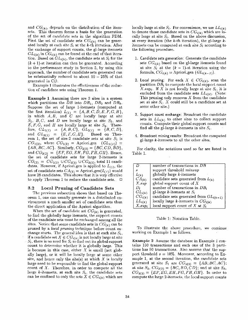
and CG(k), depends on the distribution of the itemsets. This theorem forms a basis for the generation of the set of candidate sets in the algorithm FDM. First the set of candidate sets CG!i(k) can be generated locally at each site Si at the k-th iteration. After the exchange of support counts, the gl-large itemsets GLqk) in CGi(k) can be found at the end of that iteration. Based on GL;(k), the candidate sets at Si for the (k + 1)-st iteration can then be generated. According to the performance study in Section 5, by using this approach, the number of candidate sets generated can be substantially reduced to about 10 - 25% of that generated in CD.

Example 1 illustrates the effectiveness of the reduction of candidate sets using Theorem 1.

Example 1 Assuming there are 3 sites in a system which partitions the DB into DB1, DB2 and DB3. Suppose the set of large 1-itemsets (computed at the first iteration) L(1) = { A , B , C , D , E , F ,G,H} , in which A, B , and C are locally large at site S I , I?, 6, and D are locally large at site S2, and E , F,C, and H are locally large att site S3. There- fore, G I q l ) = ( A , B , C } , GL2(1) = { B , C , D} , and GL3(1) = {E ,F ,G , H } . Based on Theo- rem I , the set of size-2 candidate sets at site SI is CG1(2), where CGI(2) = Apriori.gen (GLI(1) ) = ( A B , BC, AC}. Similarly, CG2(2) = {BC, CD, BD}, and CG3(2) = {EF, EG, EH, FG, FH,GH}. Hence, the set of candidate sets for large 2-itemsets is CG(2) = CGl(2) U CGZ(2) U CG3(2), total 11 candidates. However, if Apriori-gen is applied to L(1), the set of candidate sets CA(2) = Apriori-gen(L(l)) would have 28 candidates. This shows that it is very effective to apply Theorem 1 to reduce the candidate sets. 0

3.2 Local Pruning of Candidate Sets The previous subsection shows that based on The-

orem 1, one can usually generate in a distributed environment a much smaller set of candidate sets than the direct application of the Apriori algorithm.

When the set of candidate set C'G(k) is generated, to find the globally large itemsets, i,he support counts of the candidate sets must be exchainged among all the sites. Notice that some candidate sets in CG(k) can be pruned by a local pruning technique before count exchange starts. The general idea is that at each site Si, if a candidate set X E CG,(k) is not locally large at site Si, there is no need for S, to find out its global support count to determine whether it is gllobally large. This is because in this case, either X is small (not globally large), or it will be locally large at some other site, and hence only the site(s) at which X is locally large need to be responsible to find the global support count of X . Therefore, in order to compute all the large k-itemsets, at each site Si, the candidate sets can be confined to only the sets X E CGi(k) which are

locally large at site Si. For convenience, we use LL;(k) to denote those candidate sets in CGi(k) which are locally large at site Si. Based on the above discussion, at every iteration (the k-th iteration), the gl-large k- itemsets can be computed at each site Si according to the following procedure.

1. Candidate sets generation: Generate the candidate sets CGi(k) based on the gl-large itemsets found at site Si at the ( k - 1)-st iteration using the formula, CG;(k) = Apriori-gen ( GLz(k- l ) ) .

2. Local pruning: For each X E CGi(k), scan the partition DBi to compute the local support count X.supi. If X is not locally large at site Si, it is excluded from the candidate sets & ( k ) . (Note: This pruning only removes X from the candidate set at site Si. X could still be a candidate set at some other site.)

3. Support count exchange: Broadcast the candidate sets in LL;(k) to other sites to collect support counts. Compute their global support counts and find all the gl-large k-itemsets in site Si.

4. Broadcast min ing results: Broadcast the computed gl-large k-itemsets to all the other sites.

For clarity, the notations used so far are listed in Table 1.

number of transactions in DB support threshold minsup globally large k-itemsets candidate sets generated from L ( k ) global support count of X number of transactions in DBi gl-large k-itemsets at Si candidate sets generated from GLi(k-1) locally large k-itemsets in CGi(k) local support count of X at Si

Table 1: Notation Table.

To illustrate the above procedure. we continue working on Example 1 as follows.

Example 2 Assume the database in Example 1 contains 150 transactions and each one of the 3 partitions has 50 transactions. Also assume that the support threshold s = 10%. Moreover, according to Ex- ample 1, at the second iteration, the candidate sets generated at site SI are CG1(2) = {AB, BC,AC}; at site S2, CGq2) = {BC, BD, CD}; and at site S3, CG3(2) = (EF, EG, EH, FG, F H , GH}. In order to compute the large 2-itemsets, the local support counts

34

Table 2: Locally Large Itemsets.

large request candidates from

AB s1 BC Sl , s2 CD s2 EF s3 GH s3

at each site is computed first. The result is recorded in Table 2.

From Table 2, it can be seen that AC.sup1 = 2 < s x D1 = 5. AC is not locally large. Hence, the candidate set AC is pruned away at site S I . On the other hand, both A B and BC have enough local s u p port counts and they survive the local pruning. Hence LLq2) = { A B , BC}. Similarly, LL2(2) = {BC, CD}, and LL3(2) = { E F , GH}. After the local pruning, the number of size-2 candidate sets has been reduced to five which is less than half of the original size. Once the local pruning is completed, each site broadcasts messages containing all the remaining candidate sets to the other sites to collect their support counts. The result of this count support exchange is recorded in Table 3.

1

5 4 4 10 10 2 4 8 4 4 3 8 4 4 6

Table 3: Globally Large Itemsets.

The request for support count for AB is broadcasted from SI to site S2 and 5’3, and the counts sent back are recorded at site S1 as in the second row of Table 3. The other rows record similar count exchange activities at the other sites. At the end of the iteration, site S1 finds out that only BC is gl- large, because BC.sup = 22 > s x D = 15, and AB.sup = 13 < s x D = 15. Hence the gl-large 2-itemset a t site S1 is GLl(2) = {BC}. Similarly, GL2(2) = {BC,CD} and GL3(2) = { E F } . After the broadcast of the gl-large itemsets, all sites return the large 2-itemsets 4 2 ) = {BC, CD, E F } .

Notice that some candidate set, such as BC in this example, could be locally large at more than one site. In this case, the messages are broadcasted from all the

sites at which BC is found to be locally large. This is unnecessary because for each of candidate itemset, only one broadcast is needed. In Section 3.4, an optimization technique to eliminate such redundancy will be discussed. 0

There is a subtlety in the implementation of the four steps outlined above for finding globally large itemsets. In order to support both step 2, “local pruning”, and step 3, “support count exchange”, each site Si must have two sets of support counts. For local pruning, Si has to find the local support counts of its candidate sets CGi(k). For support count exchange, Si has to find the local support counts of some possi- bly different candidate sets from other sites in order to answer the count requests from these sites. A simple approach would be to scan DBi twice, once for collection of the counts for the local CGqk), and once for responding to the count requests from other sites. However, this would substantially degrade the performance.

At Si, not only is CG;(k) available at the beginning of the H-th iteration, but also are other sets, i.e., CGj(k) ( j = 1 , . . . , n, j # i), because all the GLi(k-l), (i = 1 , . . . , n), are broadcasted to every site at the end of the (H - 1)-st iteration, and the sets of candidate sets CGqk), (i = 1, . . . , n) , are computed from the corresponding GLi(k-1). That is, at the beginning of each iteration, since all the gl-large itemsets found at the previous iteration have been broadcasted to all the sites, every site can compute the candidate sets of every other site. Therefore, the local support counts of all these candidate sets can be found in one scan and stored in a data structure like the hash-tree used in Apriori [2]. Using this technique, the data structure can be built in one scan, and the two different sets of support counts required in the local pruning and support count exchange can be retrieved from this data structure. 3.3 Global Pruning of Candidate Sets

The local pruning at a site Si uses only the local support counts found in DBi to prune a candidate set. In fact, the local support counts from other sites can also be used for pruning. A global pruning technique is developed to facilitate such pruning and is outlined as follows. At the end of each iteration, all the local support and global support counts of a candidate set X are available. These local support counts can be broadcasted together with the global support counts after a candidate set is found to be globally large. Using this information, some global pruning can be performed on the candidate sets at the subse- quent iteration.

Assume that the local support count of every candidate itemset is broadcasted to all the sites after it is found to be globally large at the end of an itera-

In fact, there is no need of two scans.

35

tion. Suppose X is a size-k candidiate itemset at the k-th iteration. Therefore, the local support counts of all the size-(k - 1) subsets of X are available at every site. With respect to a partition DBi , (1 5 i 5 n) , we use mazsup i (X) to denote the minimum value of the local support counts of all the size-(k - 1) subsets of X , i.e, m a z s u p i ( X ) = min{Y.supi I Y c X and IYI = k - 1). It follows from the subset relationship that mazsup i (X) is a n upper bound of the local support count X.supi. Hence, the sum of these upper bounds over all partitions, denoted by m a z s u p ( X ) , is an upper bound of X.sup. In other words, X.sup 5 maxsup(X) = mazsup i (X) . Note that m a z s u p ( X ) can be computed at every site at the beginning of the k-th iteration. Since m a z s u p ( X ) is an upper bound of its global support count, it can be used for pruning, i.e., if mazsup(X) < s x D, then X cannot be a candidate itemset. This technique is called global pruning.

Global pruning can be combined with local pruning to form different pruning strategies. Two particular variations of this strategy will be adopted when we introduce several versions of FDM in Section 4. The first method is called upper-boundpruning and the second one is called polling-site-pruning. We will discuss the upper-bound-pruning met hod here in detail. The polling-site-pruning method will be explained in Subsection 4.3. In the upper-boundl-pruning, a site Si first uses the techniques in Subsections 3.1 and 3.2 to generate and perform local pruning on the candidate sets. Before count exchange starts, the site Si applies global pruning to the remaining candidate sets. A possible upper bound of the global support count of a candidate set X is the sum

x.supi + 2 m a z s u p j ( X ) . j=1 ,j#i

where X.supi is found already iin the local pruning. Therefore, this upper bound can be computed to prune the candidate set X at site Si.

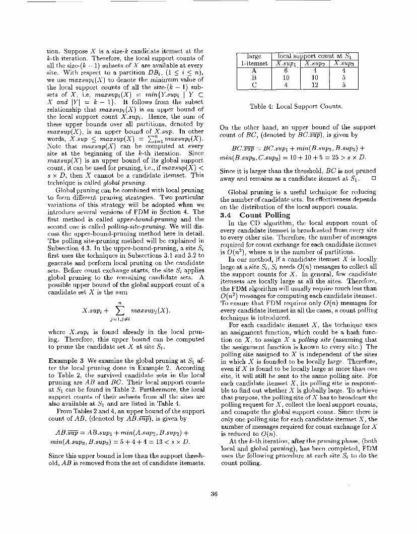
Example 3 We examine the global pruning at S1 after the local pruning done in Example 2. According to Table 2, the survived candidate sets in the local pruning are AB and BC. Their lolcal support counts at SI can be found in Table 2. Furthermore, the local support counts of their subsets from all the sites are also available at SI and are listed in Table 4.

From Tables 2 and 4, an upper bound of the support count of A B , (denoted by AB.-), is given by

A B . W = AB.sup1 + min(A.sup2, B.sup2) + min(A.sup3, B . s u ~ ~ ) = 5 + 4 + 4 =I 13 < s x D.

Since this upper bound is less than the support threshold, AB is removed from the set of candidate itemsets.

large 1-itemset

A

local support count at S1 X.supl 1 X.sup2 I X.sup3

6 I 4 4 B C

Table 4: Local Support Counts.

10 10 5 4 12 5

On the other hand, an upper bound of the support count of BC, (denoted by B C . W ) , is given by

B C . W = BC.sup1 + min(B.sup2, B.sup2) + min(B.sup3, C . S U ~ Q ) = 10 + 10 + 5 = 25 > s x D.

Since it is larger than the threshold, BC is not pruned away and remains as a candidate itemset at SI. 0

Global pruning is a useful technique for reducing the number of candidate sets. Its effectiveness depends on the distribution of the local support counts. 3.4 Count Polling

In the CD algorithm, the local support count of every candidate itemset is broadcasted from every site to every other site. Therefore, the number of messages required for count exchange for each candidate itemset is O(n2) , where n is the number of partitions.

In our method, if a candidate itemset X is locally large at a site Si, Si needs O(n) messages to collect all the support counts for X . In general, few candidate itemsets are locally large at all the sites. Therefore, the FDM algorithm will usually require much less than O(n2) messages for computing each candidate itemset. To ensure that FDM requires only O(n) messages for every candidate itemset in all the cases, a count polling technique is introduced.

For each candidate itemset X , the technique uses an assignment function, which could be a hash function on X , to assign X a polling site (assuming that the assignment function is known to every site.) The polling site assigned to X is independent of the sites in which X is founded to be locally large. Therefore, even if X is found to be locally large at more than one site, it will still be sent to the same polling site. For each candidate itemset X , its polling site is responsible to find out whether X is globally large. To achieve that purpose, the polling site of X has to broadcast the polling request for X , collect the local support counts, and compute the global support count. Since there is only one polling site for each candidate itemset X , the number of messages required for count exchange for X is reduced to O(n) .

At the k-th iteration, after the pruning phase, (both local and global pruning), has been completed, FDM uses the following procedure at each site Si to do the count polling.

36

1. Send candidate sets to polling sites: At site Si, for every polling site Sj, find all the candidate itemsets in LLi(k) whose polling site is Sj and store them in LLi,j(k) (i.e., candidates are being put into groups by their polling sites). The local support counts of the candidate itemsets are also stored in the corresponding set LLi,j(k). Send each L L i , j ( k ) to the corresponding polling site Sj.

2. Poll and collect support counts: If Si is a polling site, Si receives all LLj,i(k) sent to it from the other sites. For every candidate itemset X received, Si finds the list of originating sites from which X is being sent. Si then broadcasts the polling requests to the other sites not on the list to collect the support counts.

3. Compute gl-large itemsets: Si receives the support counts from the other sites, computes the global support counts for its candidates, and finds the gl- large itemsets. Eventually, Si broadcasts the gl- large itemsets together with their global support counts to all the sites.

Example 4 In Example 2, assuming that S1 is assigned as the polling site of A B and B C , Sz is assigned as the polling site of CD, and S, is assigned as the polling site of EF and GH.

Following from the assignment, site S1 is responsible for the polling of A B and B C . In the simple case of A B , Si sends polling requests to Sz and S3 to collect the support counts. As for B C , it is locally large at both Si and Sz, the pair (BC, BC.supz) = ( B C , 10) is sent to Si by Sz. After SI receives the message, it sends a polling request to the remaining site 5’3. Once the support count BC.sup3 = 2 is received from S3, Si finds out that BC.sup = 10 + 10 i- 2 = 22 > 15. Hence B C is a gl-large itemset at S i . In this example, with a polling site, the double polling messages for B C has been eliminated. cl

4 Algorithm for Distributed Mining of Association Rules

In this section, the basic version of FDM, i.e., the FDM-LP (FDM with Local Pruning) algorithm, is first presented, which adopts two techniques: candidate set reduction and local pruning, discussed in Sec- tion 3. According to our performance study in Sec- tion 5, FDM-LP is much more efficient than CD. 4.1 The FDM-LP algorithm Algorithm 1 FDM-LP: FDM with Local Prun- ing

Input: DBi (i = 1 , . . . , n): the database partition at each site Si.

Output: L: the set of all globally large itemsets.

Method: Iteratively execute the following program fragment (for the k-th iteration) distributively at each site Si. The algorithm terminates when either L ( k ) = 0, or the set of candidate sets CG(k) = 0.

(1) (2) z(1) = get-local-count(DBi, 0 , l ) (3) else {

if k = 1 then

(4) CG(k) = UZ“=,Gf(k). = Uin,,Aprzorz-gen(GLi(k-l));

q ( k ) = get-local-count(DBi, CG(k), i) ; }

if X.supi 2 s x Di then for j = 1 to n do

(5) (6) (7)

for-all X E q ( k ) do

if polling-site(X) = Sj then (8) (9)

insert ( X , X.supi) into LLi,j(k); (10) for j = 1 , . . . , n do send LLi,j(k) to site Sj; (11) for j = 1, . . . , n do { (12) receive LLj,i(k);

(13) for-all X E LLj,i(k) do { if X $2 LPqk) then

insert X into LPqk); (14)

(15) update X.large-sites; } } (16) for-all X E LPi(b) do (17) send-pollzng-request ( X ) ; (18) reply-pol l ing-reques t (~(k) ) ; (19) for-all X E LPi(k) do { (20) receive X.supj from the sites Sj ,

where Sj # X.largesites;

if X.sup 2 s x D then (21) x . s u p = cy=l x.supi; (22)

(23) broadcast Gqk); (24) receive Gj(k) from all other sites Sj, ( j # i);

(26) divide L ( k ) into GLi(k), (i = 1 , . . . , n) ; (27) return L ( k ) .

insert X into G q k ) ; }

(25) L ( k ) = UY=IGi(k).

Explanation of Algorithm 1 In Algorithm 1, every site Si is initially a “home

site” of a set of candidate sets that it generates. Later, it becomes a polling site to serve the requests from other sites. Subsequently, it changes its status to a remote site to supply local support counts to other polling sites. The corresponding steps in Algorithm 1 for these different roles and activities are grouped and explained as the follows.

1. H o m e site: generate candidate sets and submit them to polling sites (lines 1 - 10).

At the first iteration, the site Si calls get-local-count to scan the partition DBi once and store the local support counts of all the 1- itemsets found in the array q(1). At the k-th (for

37

2.

3.

4.

5.

k > 1) iteration, Si first compultes the set of candidate set CG(k), and then scans DBj to build the hash tree ?;:(k) containing the locally support counts of all the sets in CG(1,). By traversing T i ( k ) , Si finds out all locally large k-itemsets and group them according to their polling sites. Fi- nally, it sends the candidate sets with their local support counts to their polling sites.

Polling site: receive candidate sets and send polling requests (lines 11 - 17). As a polling site, site Si receives candidate sets from the other sites and insert them in LPip). For each candidate set X E LP,(k , S, stores all its “home” sites in X.large-sites, w h ich contains all those sites from which X is sent to Si for polling. In order to perform count exchange for X , S, calls sendqolling-request to send X to those sites not in the list X.large-sites to colliect the remaining support counts.

Remote site: return support counts to polling site (line 18). When Si receives polling requests from the other sites, it acts as a remote site. For each candidate set Y it receives from a polling site, it retrieves Y.supi from the hash tree x ( k ) and returns it to the polling site.

Polling site: receive support counts and find large itemsets (lines 19 - 23 ). As a polling site, Si receives the local support counts for the candidate sets in LPi(k). Following that, it computes the global support counts of all these candidate sets and find out the globally large itemsets among them. These globally large k-itemsets are stored in the set Gi(k). Finally, Si broadcasts the set Gqk) to all the other sites.

H o m e site: receive large itemsets (lines 24 - 27).

As a “home” site, Si receives the sets of globally large k-itemsets Gl(k) from all the polling sites. By taking the union of G,(k), ( i = 1 , . . .,n), Si finds out the set Lk of all the size-k large itemsets. Further, S, finds out from L k the set GLi(k) of gl- large itemsets for each site by using the site list in X.darge-sites. The sets GLi(k) will be used for candidate set generation at the next iteration. 0

4.2 The FDM-LUP algorithm Algorithm 2 FDM-LUP: FDM with Local and Upper-Bound-Pruning

Method: The program fragment of FDM-LUP is ob- tained from FDM-LP by inserting the following condition (line 7.1) after line 7 of Algorithm 1.

(7.1) if g-upperhound(X) 2 s x D then

Explanation of Algorithm 2 The only new step in FDM-LUP is the one

for upper-bound-pruning (line 7.1). The function g-upper-bound computes an upper bound for a candidate set X according to the formula suggested in Subsection 3.3. In other words, g-upper-bound returns an upper bound of X as the sum

n

x .supi + muzsupJ ( X ) . j=1 , j # i

As explained in Subsection 3.3, X.supi is computed already in the local pruning step, and the values of m a z s u p j ( X ) , ( j = 1 , . . . , n, j # i ) , can be computed from the local support counts from the ( k - 1)-st iteration. If this upper bound is smaller than the global support threshold, it is used to prune away X . FDM- LUP should usually have a smaller number of candidate sets for count exchange in comparison with FDM- LP. 0

4.3 The FDM-LPP algorithm Algorithm 3 FDM-LPP: FDM with Local Pruning and Polling-Site-Pruning

Method: The program fragment of FDM-LPP is ob- tained from Algorithm 1 by replacing its line 17 with the following two lines.

(16.1) (17) send-polling-request ( X ) ;

if p-upper-bound(X) 2 s x D then

Explanation of Algorithm 3 The new step in FDM-LPP is the one for polling-

site-pruning (line 16.1). At that stage, Si is a polling site and has received requests from the other sites to perform polling. Each request contains a locally larEe itemset X and its local sumort count X.sup;.

-.I, _ _ The FDM-LP described above has utilized the tech-

niques described in Subsections 3.1, 3.2, and 3.4. An illustration of FDM-LP by example can be found in Examples 1, 2 and 3 together.

In the following, two refinements of FDM-LP, by adoption of different global pruning techniques, are presented.

where Sj is a site from which X is sent to Si. Note that X.large-sites is the set of all the originating sites from which the requests for polling X are being sent to the polling site (line 15). For every site Sj E X.large-sites, the local support count X.supj has been sent to Si already. For a site S, X.Zarge-sites, since X is not locally large at S,, its

38

local support count X.sup, must be smaller than the local threshold s x D,. Following from the discussion in Subsection 3.3, X.supq is bounded by the value min(maxsupq ( X ) , s x D, - 1). Hence an upper bound of X.sup can be computed by the sum

x .supj + jEX.large-sites

2 min(mazsupq(X) , s x Dq - 1). q = l ,q+?X.large-sites

In FDM-LPP, Si calls p-upper-bound to compute an upper bound for X.sup according to the above formula. This upper bound can be used to prune away X if it is smaller than the global support threshold.

0 As discussed before, both FDM-LUP and FDM-

LPP may have less candidate sets than FDM-LP. How- ever, they require more storage and communication messages for the local support counts. Their efficiency comparing with FDM-LP will depend largely on the data distribution.

5 Performance Study of FDM An in-depth performance study has been performed

to compare FDM with CD. We have chosen to im- plement the representative version of FDM, FDM- LP, and compare it against CD. Both algorithms are implemented on a distributed system by using PVM (Parallel Virtual Machine) [6]. A series of three to six RS/6000 workstations, running the AIX system, are connected by a 10Mb LAN to perform the experiment. The databases in the experiment are composed of synthetic data.

In the experiment result, the number of candidate sets found in FDM at each site is between 10 - 25% of that in CD. The total message size in FDM is between 10 - 15% of that in CD. The execution time of FDM is between 65 - 75% of that in CD. The reduction in the number of candidate sets and message size in FDM is very significant. The reduction in execution time is also substantial. However, it is not directly proportional to the reduction in candidate sets and message size. This is mainly due to the overhead of running FDM and CD on PVM. What we have observed is that the overhead of PVM in FDM is very close to that in CD, even though the amount of message communication is significantly smaller in FDM. From the results of our experiments, it is also clear that the performance gain of FDM over CD will be higher in distributed systems in which the communication bandwidth is an important performance factor. For example, if the mining is being done on a distributed database over wide area or long haul network. The performance of FDM-LP against Apriori in a large database is also compared. In that case, the response time of FDM-LP is only about 20% longer

Interpretation transaction mean size mean size of maximal potentially large itemsets number of potentially large itemsets Number of items Clustering size Pool size Correlation level Multiplying factor

Parameter ITI I I I

I L I

N sq Ps

Mf Cr

Value 10 4

2000

1000 5 - 6 50 - 70 0.5 1260 - 2400

Table 5: Parameter Table.

than 1/n of the response time of Apriori, where n is the number of sites. This is a very ideal speed-up. In terms of total execution time, FDM-LP is very close to Apriori.

The test bed that we use has six workstations. Each one of them has its own local disk, and its partition is loaded on its local disk before the experiment starts. The databases used in our experiment are synthetic data generated using the same techniques introduced in [2, lo]. The parameters used are similar to those in [lo]. Table 5 is a list of the parameters and their values used in our synthetic databases. Readers not familiar with these parameters can refer to [2, lo]. In the following, we use the notation Tx.Iy.Dm to denote a database in which D = m (in thousands), IT1 = x, and 111 = y.

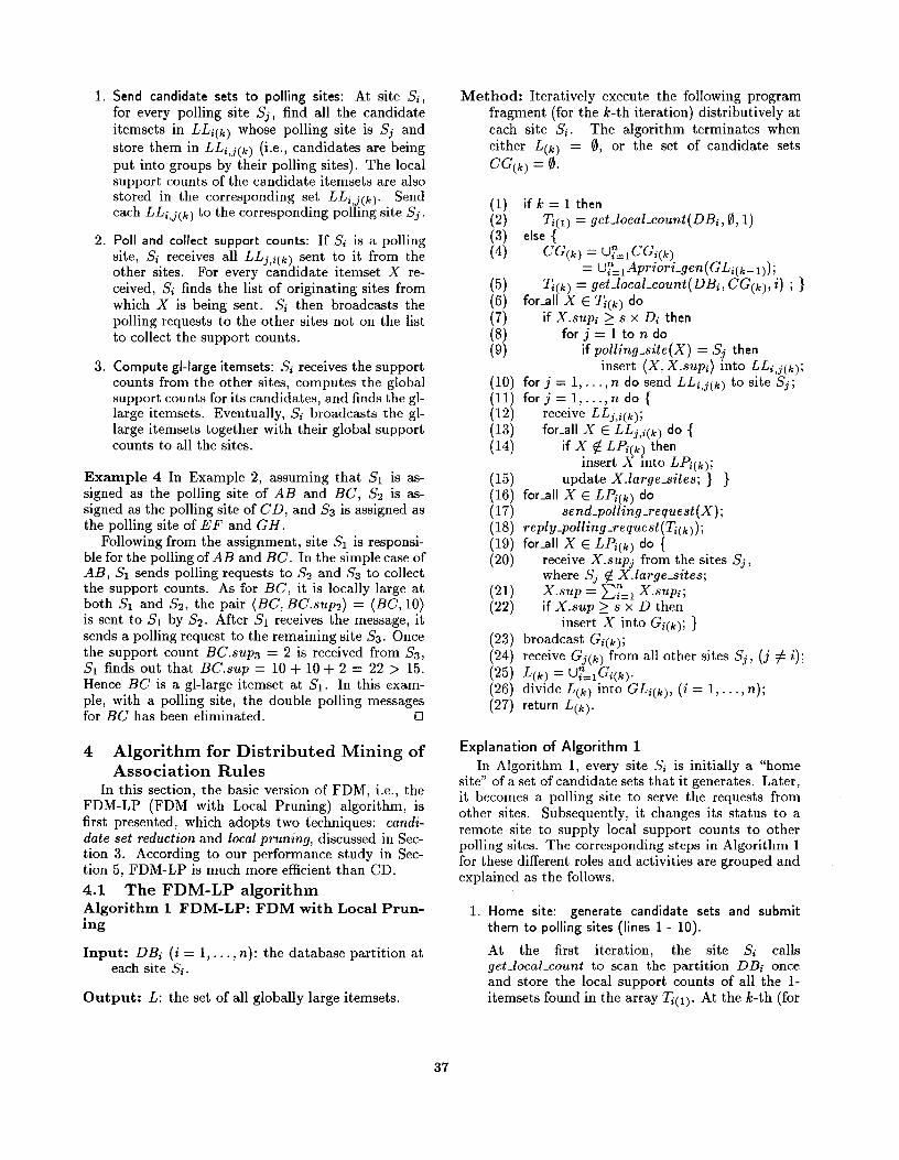
T10.14.D200K, s = 3%

4 5 6 Number of Nodes

+FDM +CD

Figure 1: Candidate Sets Reduction (n = 3, 4, 5, 6)

5.1 Candidate Sets and Message Size Re- duction

The sizes of the databases in our study range from 200K to 600K transactions, and the minimumsupport threshold ranges from 3% to 3.75%. Note that the number of candidate sets at each site are the same in CD and different in FDM. In our experiment, we witnessed a reduction of 75 - 90% of candidate sets on

39

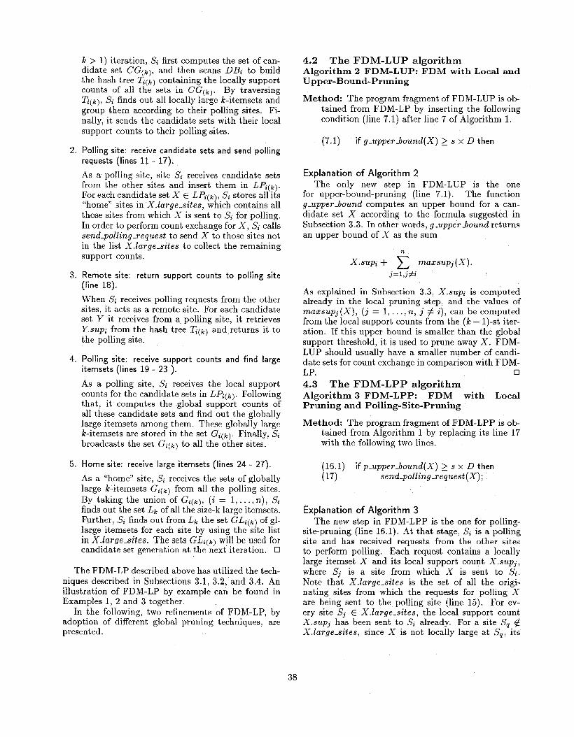
T10.14.D200K, n = 3 T10.14.D200K, n = 3

60 , I

S 8 3.00 3.25 3.510 3.75 YO % %I YO

Minimum support +FDM + k C D

~ g s 3.00% 3.25% 3.50% 3.75%

Minimum support

+FDM +CD

Figure 4: Message Size Reduction Figure 2: Candidate Sets Reduction

average at each site when FDM-LP is compared with CD. In Figure 1, the average number of candidate sets generated by FDM-LP and CD for a 200K transaction database are plotted against the number of partitions. FDM-LP has a 75 - 90% reduction in the candidate sets. The percentage of reduction increases when the number of partitions increases. This shows that FDM becomes more effective when the system is scaled up. In Figure 2, the same comparison between FDM-LP and CD is presented for the same database with three partitions on different thresholds. In this case, FDM- LP experienced a similar amount of reduction.

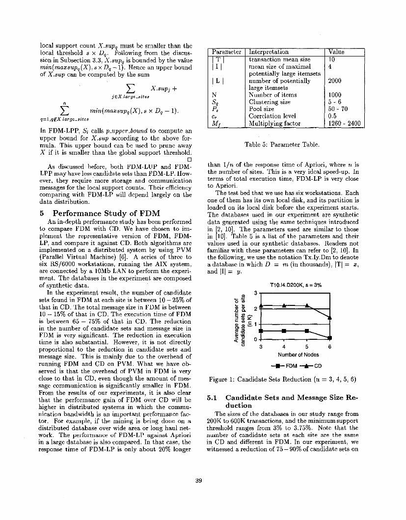
T10.14.D200K, s = 30/0

I-

150

100

50

0 3 4 5 6

Number of Nodos

+FDM +CB

Figure 3: Message Size Reduction (n = 3, 4, 5 , 6)

The reduction in candidate sets should have a proportional impact on the reduction (of messages in the comparison. Moreover, as discussed before, the polling site technique guarantees that FDM only requires O(n) messages for each candidate set, which is much smaller than the O ( n 2 ) messages required in CD. In our experiment, FDM has about 90% reduction in the total message size in all cases when it is compared with CD. In Figure 3, the total message size in FDM and CD for the same 200K database are plotted against the number of partitions. In Figure 4, the same comparison on the same database of three partitions with dif-

ferent support thresholds are presented. Both results confirm our analysis that FDM-LP is very effective in cutting down the number of messages required.

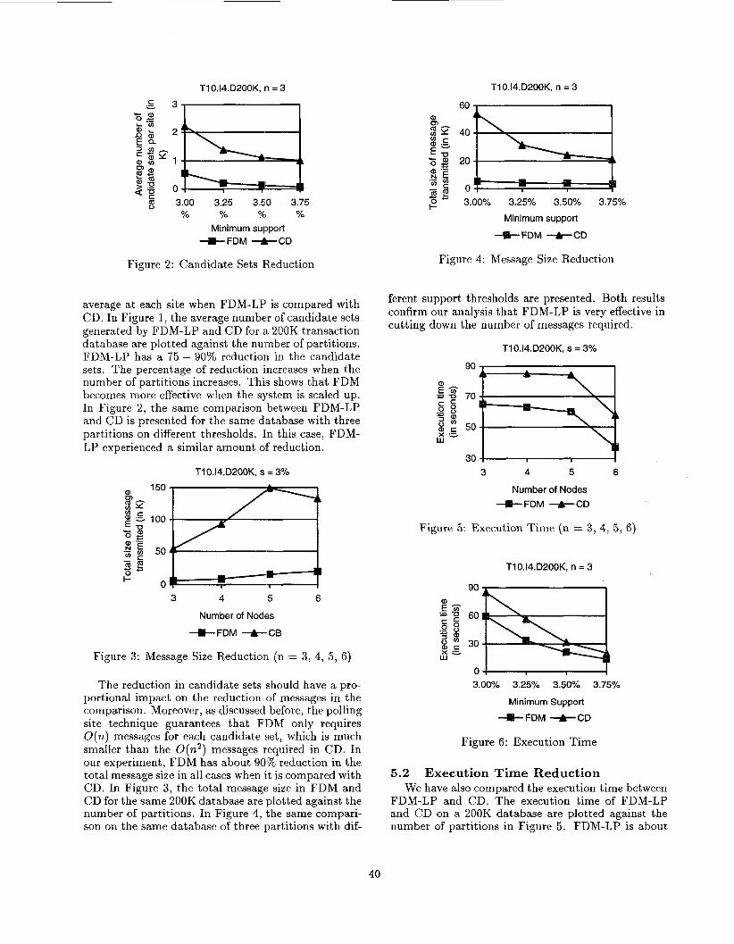
T10.14.D200K, s = 3%

90

E 3

2 8

.= U 70 c c .Q 8 a c 50 c

x s w

"" I

3 4 5 6

Number of Nodes +FDM +CD

Figure 5: Execution Time (n = 3, 4, 5 , 6)

T10.14.D200K, n = 3

3.00% 3.25% 3.50% 3.75%

Minimum Support

-E-FDM -A-CD

Figure 6: Execution Time

5.2 Execution Time Reduction We have also compared the execution time between

FDM-LP and CD. The execution time of FDM-LP and CD on a 200K database are plotted against the number of partitions in Figure 5. FDM-LP is about

40

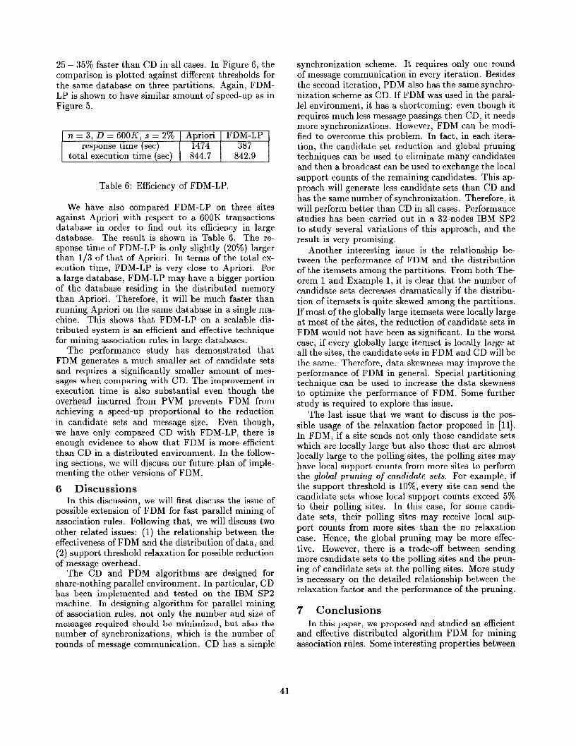
25 - 35% faster than CD in all cases. In Figure 6, the comparison is plotted against different thresholds for the same database on three partitions. Again, FDM- LP is shown to have similar amount of speed-up as in Figure 5.

n = 3, D = 60011, s = 2% I Apriori I FDM-LP response time (sec) I 1474 I 387

I total execution time (sec) I 844.7 I 842.9 I

Table 6: Efficiency of FDM-LP.

We have also compared FDM-LP on three sites against Apriori with respect to a 600K transactions database in order to find out its efficiency in large database. The result is shown in Table 6. The response time of FDM-LP is only slightly (20%) larger than 1/3 of that of Apriori. In terms of the total execution time, FDM-LP is very close to Apriori. For a large database, FDM-LP may have a bigger portion of the database residing in the distributed memory than Apriori. Therefore, it will be much faster than running Apriori on the same database in a single machine. This shows that FDM-LP on a scalable distributed system is an efficient and effective technique for mining association rules in large databases.

The performance study has demonstrated that FDM generates a much smaller set of candidate sets and requires a significantly smaller amount of messages when comparing with CD. The improvement in execution time is also substantial even though the overhead incurred from PVM prevents FDM from achieving a speed-up proportional to the reduction in candidate sets and message size. Even though, we have only compared CD with FDM-LP, there is enough evidence to show that FDM is more efficient than CD in a distributed environment. In the following sections, we will discuss our future plan of imple- menting the other versions of FDM.

6 Discussions In this discussion, we will first discuss the issue of

possible extension of FDM for fast parallel mining of association rules. Following that, we will discuss two other related issues: (1) the relationship between the effectiveness of FDM and the distribution of data, and (2) support threshold relaxation for possible reduction of message overhead.

The CD and PDM algorithms are designed for share-nothing parallel environment. In particular, CD has been implemented and tested on the IBM SP2 machine. In designing algorithm for parallel mining of association rules, not only the number and size of messages required should be minimized, but also the number of synchronizations, which is the number of rounds of message communication. CD has a simple

synchronization scheme. It requires only one round of message communication in every iteration. Besides the second iteration, PDM also has the same synchronization scheme as CD. If FDM was used in the parallel environment, it has a shortcoming: even though it requires much less message passings then CD, it needs more synchronizations. However, FDM can be modi- fied to overcome this problem. In fact, in each iteration, the candidate set reduction and global pruning techniques can be used to eliminate many candidates and then a broadcast can be used to exchange the local support counts of the remaining candidates. This approach will generate less candidate sets than CD and has the same number of synchronization. Therefore, it will perform better than CD in all cases. Performance studies has been carried out in a 32-nodes IBM SP2 to study several variations of this approach, and the result is very promising.

Another interesting issue is the relationship between the performance of FDM and the distribution of the itemsets among the partitions. From both The- orem 1 and Example 1, it is clear that the number of candidate sets decreases dramatically if the distribution of itemsets is quite skewed among the partitions. If most of the globally large itemsets were locally large at most of the sites, the reduction of candidate sets in FDM would not have been as significant. In the worst case, if every globally large itemset is locally large at all the sites, the candidate sets in FDM and CD will be the same. Therefore, data skewness may improve the performance of FDM in general. Special partitioning technique can be used to increase the data skewness to optimize the performance of FDM. Some further study is required to explore this issue.

The last issue that we want to discuss is the possible usage of the relaxation factor proposed in [ll]. In FDM, if a site sends not only those candidate sets which are locally large but also those that are almost locally large to the polling sites, the polling sites may have local support counts from more sites to perform the global pruning of candidate sets. For example, if the support threshold is lo%, every site can send the candidate sets whose local support counts exceed 5% to their polling sites. In this case, for some candidate sets, their polling sites may receive local support counts from more sites than the no relaxation case. Hence, the global pruning may be more effective. However, there is a trade-off between sending more candidate sets to the polling sites and the pruning of candidate sets at the polling sites. More study is necessary on the detailed relationship between the relaxation factor and the performance of the pruning.

7 Conclusions In this paper, we proposed and studied an efficient

and effective distributed algorithm FDM for mining association rules. Some interesting properties between

41

locally and globally large itemsets are observed, which leads to an effective technique for the reduction of candidate sets in the discovery of large itemsets. Two powerful pruning techniques, local and global prunings, are proposed. Furthermore, the optimization of the communications among the participating sites is performed in FDM using the polling sites. Sev- eral variations of FDM using different combination of pruning techniques are described. A representative version, FDM-LP, is implemented and whose performance is compared with the CD algorithm in a distributed system. The result shows the high performance of FDM at mining association rules.

Several issues related to the extensions of the method are also discussed. The techniques of candidate set reduction and global pruning can be inte- grated with CD to perform mining in a parallel environment which will be better than CD when consider- ing both message communication and synchronization. Further improvement of the performance of the FDM algorithm using the skewness of data distribution and the relaxation of support thresholds is also discussed.

Recently, there have been interesting studies on the mining of generalized association rules [14], multiple- level association rules [8], quantitative association rules [15], etc. Extension of our method to the mining of these kinds of rules in a distributed or parallel system are interesting issues for future research. Also, parallel and distributed data mining of other kinds of rules, such as characteristic rules [7], classification rules, clustering [9], etc. is an important direction for future studies. For our performance studies, an implementation of the different versions of FDM on an IBM SP2 system with 32 nodes has been carried out and the result is very promising.

References [l] R. Agrawal and J. C. Shafer. Parallel mining of

association rules: Design, implementation, and experience. In IBM Research Report, 1996.

[2] R. Agrawal and R. Srikant. Fast algorithms for mining association rules. In Proc. 1994 Int. Conf. Very Large Data Bases, pages 487-499, Santiago, Chile, September 1994.

[3] R. Agrawal and R. Srikant. Mining sequential patterns. In Proc. 1995 Int. Conf. Data Engi- neering, pages 3-14, Taipei, Taiwan, March 1995.

[4] D.W. Cheung, J . Wan, V. Ng, and C.Y. Wong. Maintenance of discovered association rules in large databases: An incremental updating technique. In Proc. 1996 Int’l Conf. on Data Engi- neering, New Orleans, Louisiana, Feb. 1996.

[5] U. M. Fayyad, 6. Piatetsky-Shapiro, P. Smyth, and R. Uthurusamy. Advances zn Knowledge Dis- covery and Data Mining. AAAI/MIT Press, 1996.

[6] A. Geist, A. Beguelin, J . Dongarra, W. Jiang, R. Manchek, and V. Sunderam. PVM: Parallel Virtual Machine, A Users’ Guide and Tutorial

for Networked Parallel Computing. MIT Press, 1994.

[7] J . Han, Y, Cai, and N. Cercone. Data- driven discovery of quantitative rules in relational databases. IEEE Trans. Knowledge and Data En- gineering, 5:29-40, 1993.

Discovery of multiple-level association rules from large databases. In Proc. 1995 Int. Conf. Very Large Data Bases, pages 420-431, Zurich, Switzerland, Sept. 1995.

[8] J . Han and Y. Fu.

[9] R. Ng and J. Han. Efficient and effective clustering method for spatial data mining. In Proc. 1994 Int. Conf. Very Large Data Bases, pages 144-155, Santiago, Chile, September 1994.

[lo] J.S. Park, M.S. Chen, and P.S. Yu. An effective hash-based algorithm for mining association rules. In Proc. 1995 ACM-SIGMOD Int. Conf. Management of Data, pages 175-186, San Jose, CA, May 1995.

[ll] J.S. Park, M.S. Chen, and P.S. Yu. Efficient parallel mining for association rules. In Proc. 4th Int. Conf. on Information and Knowledge Manage- ment, pages 31-36, Baltimore, Maryland, Nov. 1995.

[12] A. Savasere, E. Omiecinski, and S. Navathe. An efficient algorithm for mining association rules in large databases. In Proc. 1995 Int. Conf. Very Large Data Bases, pages 432-443, Zurich, Switzerland, Sept. 1995.

[13] A. Silberschatz, M. Stonebraker, and J . D. U11- man. Database research: Achievements and op- portunities into the 21st century. In Report of an NSF Workshop on the Future of Database Sys- tems Research, May 1995.

[14] R. Srikant and R. Agrawal. Mining generalized association rules. In Proc. 1995 Int. Conf. Very Large Data Bases, pages 407-419, Zurich, Switzerland, Sept. 1995.

association rules in large relational tables. In Proc. 1996 ACM-SIGMOD Int. Conf. Manage- ment of Data, Montreal, Canada, June 1996.

[15] R. Srikant and R. Agrawal. Mining quantitative

42

A Fast Distributed Algorithm for Mining Association Rules

Documents

Transcript of A Fast Distributed Algorithm for Mining Association Rules