A correlated topic model of SCIENCE - arXiv

arX

iv:0

708.

3601

v2 [

stat

.AP]

31

Aug

200

7

The Annals of Applied Statistics

2007, Vol. 1, No. 1, 17–35DOI: 10.1214/07-AOAS114c© Institute of Mathematical Statistics, 2007

A CORRELATED TOPIC MODEL OF SCIENCE1

By David M. Blei and John D. Lafferty

Princeton University and Carnegie Mellon University

Topic models, such as latent Dirichlet allocation (LDA), can beuseful tools for the statistical analysis of document collections andother discrete data. The LDA model assumes that the words of eachdocument arise from a mixture of topics, each of which is a distri-bution over the vocabulary. A limitation of LDA is the inability tomodel topic correlation even though, for example, a document aboutgenetics is more likely to also be about disease than X-ray astron-omy. This limitation stems from the use of the Dirichlet distributionto model the variability among the topic proportions. In this paperwe develop the correlated topic model (CTM), where the topic pro-portions exhibit correlation via the logistic normal distribution [J.Roy. Statist. Soc. Ser. B 44 (1982) 139–177]. We derive a fast varia-tional inference algorithm for approximate posterior inference in thismodel, which is complicated by the fact that the logistic normal isnot conjugate to the multinomial. We apply the CTM to the articlesfrom Science published from 1990–1999, a data set that comprises57M words. The CTM gives a better fit of the data than LDA, andwe demonstrate its use as an exploratory tool of large document col-lections.

1. Introduction. Large collections of documents are readily available on-line and widely accessed by diverse communities. As a notable example,scholarly articles are increasingly published in electronic form, and histor-ical archives are being scanned and made accessible. The not-for-profit or-ganization JSTOR (www.jstor.org) is currently one of the leading providersof journals to the scholarly community. These archives are created by scan-ning old journals and running an optical character recognizer over the pages.JSTOR provides the original scans on-line, and uses their noisy version of

Received March 2007; revised April 2007.1Supported in part by NSF Grants IIS-0312814 and IIS-0427206, the DARPA CALO

project and a grant from Google.Supplementary material and code are available at http://imstat.org/aoas/supplementsKey words and phrases. Hierarchical models, approximate posterior inference, varia-

tional methods, text analysis.

This is an electronic reprint of the original article published by theInstitute of Mathematical Statistics in The Annals of Applied Statistics,2007, Vol. 1, No. 1, 17–35. This reprint differs from the original in pagination andtypographic detail.

1

http://arXiv.org/abs/0708.3601v2

http://www.imstat.org/aoas/

http://dx.doi.org/10.1214/07-AOAS114

http://www.imstat.org

www.jstor.org

http://lib.stat.cmu.edu/aoas/114/

http://www.imstat.org

http://www.imstat.org/aoas/

http://dx.doi.org/10.1214/07-AOAS114

2 D. M. BLEI AND J. D. LAFFERTY

the text to support keyword search. Since the data are largely unstructuredand comprise millions of articles spanning centuries of scholarly work, au-tomated analysis is essential. The development of new tools for browsing,searching and allowing the productive use of such archives is thus an impor-tant technological challenge, and provides new opportunities for statisticalmodeling.

The statistical analysis of documents has a tradition that goes back atleast to the analysis of the Federalist papers by Mosteller and Wallace [21].But document modeling takes on new dimensions with massive multi-authorcollections such as the large archives that now are being made accessibleby JSTOR, Google and other enterprises. In this paper we consider topic

models of such collections, by which we mean latent variable models of doc-uments that exploit the correlations among the words and latent semanticthemes. Topic models can extract surprisingly interpretable and useful struc-ture without any explicit “understanding” of the language by computer. Inthis paper we present the correlated topic model (CTM), which explicitlymodels the correlation between the latent topics in the collection, and en-ables the construction of topic graphs and document browsers that allow auser to navigate the collection in a topic-guided manner.

The main application of this model that we present is an analysis of theJSTOR archive for the journal Science. This journal was founded in 1880by Thomas Edison and continues as one of the most influential scientificjournals today. The variety of material in the journal, as well as the largenumber of articles ranging over more than 100 years, demonstrates the needfor automated methods, and the potential for statistical topic models toprovide an aid for navigating the collection.

The correlated topic model builds on the earlier latent Dirichlet allocation(LDA) model of Blei, Ng and Jordan [8], which is an instance of a generalfamily of mixed membership models for decomposing data into multiple la-tent components. LDA assumes that the words of each document arise froma mixture of topics, where each topic is a multinomial over a fixed wordvocabulary. The topics are shared by all documents in the collection, butthe topic proportions vary stochastically across documents, as they are ran-domly drawn from a Dirichlet distribution. Recent work has used LDA as abuilding block in more sophisticated topic models, such as author-documentmodels [19, 24], abstract-reference models [12] syntax-semantics models [16]and image-caption models [6]. The same kind of modeling tools have alsobeen used in a variety of nontext settings, such as image processing [13, 26],recommendation systems [18], the modeling of user profiles [14] and themodeling of network data [1]. Similar models were independently developedfor disability survey data [10, 11] and population genetics [22].

In the parlance of the information retrieval literature, LDA is a “bag ofwords” model. This means that the words of the documents are assumed to

A CORRELATED TOPIC MODEL OF SCIENCE 3

be exchangeable within them, and Blei, Ng and Jordan [8] motivate LDAfrom this assumption with de Finetti’s exchangeability theorem. As a con-sequence, models like LDA represent documents as vectors of word countsin a very high dimensional space, ignoring the order in which the words ap-pear. While it is important to retain the exact sequence of words for readingcomprehension, the linguistically simplistic exchangeability assumption isessential to efficient algorithms for automatically eliciting the broad seman-tic themes in a collection.

The starting point for our analysis here is a perceived limitation of topicmodels such as LDA: they fail to directly model correlation between topics.In most text corpora, it is natural to expect that subsets of the underlyinglatent topics will be highly correlated. In Science, for instance, an articleabout genetics may be likely to also be about health and disease, but un-likely to also be about X-ray astronomy. For the LDA model, this limitationstems from the independence assumptions implicit in the Dirichlet distri-bution on the topic proportions. Under a Dirichlet, the components of theproportions vector are nearly independent, which leads to the strong andunrealistic modeling assumption that the presence of one topic is not corre-lated with the presence of another. The CTM replaces the Dirichlet by themore flexible logistic normal distribution, which incorporates a covariancestructure among the components [4]. This gives a more realistic model ofthe latent topic structure where the presence of one latent topic may becorrelated with the presence of another.

However, the ability to model correlation between topics sacrifices someof the computational conveniences that LDA affords. Specifically, the con-jugacy between the multinomial and Dirichlet facilitates straightforwardapproximate posterior inference in LDA. That conjugacy is lost when theDirichlet is replaced with a logistic normal. Standard simulation techniquessuch as Gibbs sampling are no longer possible, and Metropolis–Hastingsbased MCMC sampling is prohibitive due to the scale and high dimensionof the data.

Thus, we develop a fast variational inference procedure for carrying outapproximate inference with the CTM model. Variational inference [17, 29]trades the unbiased estimates of MCMC procedures for potentially biasedbut computationally efficient algorithms whose numerical convergence iseasy to assess. Variational inference algorithms have been effective in LDAfor analyzing large document collections [8]. We extend their use to theCTM.

The rest of this paper is organized as follows. We first present the corre-lated topic model and discuss its underlying modeling assumptions. Then,we present an outline of the variational approach to inference (the techni-cal details are collected in the Appendix) and the variational expectation–maximization procedure for parameter estimation. Finally, we analyze the


performance of the model on the JSTOR Science data. Quantitatively, weshow that it gives a better fit than LDA, as measured by the accuracy of thepredictive distributions over held out documents. Qualitatively, we presentan analysis of all of Science from 1990–1999, including examples of topicallyrelated articles found using the inferred latent structure, and topic graphsthat are constructed from a sparse estimate of the covariance structure ofthe model. The paper concludes with a brief discussion of the results andfuture work that it suggests.

2. The correlated topic model. The correlated topic model (CTM) is ahierarchical model of document collections. The CTM models the words ofeach document from a mixture model. The mixture components are sharedby all documents in the collection; the mixture proportions are document-specific random variables. The CTM allows each document to exhibit mul-tiple topics with different proportions. It can thus capture the heterogeneityin grouped data that exhibit multiple latent patterns.

We use the following terminology and notation to describe the data, latentvariables and parameters in the CTM.

• Words and documents. The only observable random variables that weconsider are words that are organized into documents. Let wd,n denotethe nth word in the dth document, which is an element in a V -term vo-cabulary. Let wd denote the vector of Nd words associated with documentd.

• Topics. A topic β is a distribution over the vocabulary, a point on theV − 1 simplex. The model will contain K topics β1:K .

• Topic assignments. Each word is each assumed drawn from one of the Ktopics. The topic assignment zd,n is associated with the nth word and dthdocument.

• Topic proportions. Finally, each document is associated with a set of topic

proportions θd, which is a point on the K−1 simplex. Thus, θd is a distri-bution over topic indices, and reflects the probabilities with which wordsare drawn from each topic in the collection. We will typically consider anatural parameterization of this multinomial η = log(θi/θK).

Specifically, the correlated topic model assumes that an N -word documentarises from the following generative process. Given topics β1:K , a K-vectorµ and a K ×K covariance matrix Σ:

1. Draw ηd|{µ,Σ} ∼N (µ,Σ).2. For n ∈ {1, . . . ,Nd}:

(a) Draw topic assignment Zd,n|ηd from Mult(f(ηd)).(b) Draw word Wd,n|{zd,n,β1:K} from Mult(βzd,n

),


Fig. 1. Top: Probabilistic graphical model representation of the correlated topic model.The logistic normal distribution, used to model the latent topic proportions of a document,can represent correlations between topics that are impossible to capture using a Dirichlet.Bottom: Example densities of the logistic normal on the 2-simplex. From left: diagonalcovariance and nonzero-mean, negative correlation between topics 1 and 2, positive corre-lation between topics 1 and 2.

where f(η) maps a natural parameterization of the topic proportions to themean parameterization,

θ = f(η) =exp{η}∑i exp{ηi}

.(1)

(Note that η does not index a minimal exponential family. Adding anyconstant to η will result in an identical mean parameter.) This process isillustrated as a probabilistic graphical model in Figure 1. (A probabilistic

graphical model is a graph representation of a family of joint distributionswith a graph. Nodes denote random variables; edges denote possible depen-dencies between them.)

The CTM builds on the latent Dirichlet allocation (LDA) model [8]. La-tent Dirichlet allocation assumes a nearly identical generative process, butone where the topic proportions are drawn from a Dirichlet. In LDA andits variants, the Dirichlet is a computationally convenient distribution overtopic proportions because it is conjugate to the topic assignments. But, theDirichlet assumes near independence of the components of the proportions.In fact, one can simulate a draw from a Dirichlet by drawing from K inde-pendent Gamma distributions and normalizing the resulting vector. (Note


that there is slight negative correlation due to the constraint that the com-ponents sum to one.)

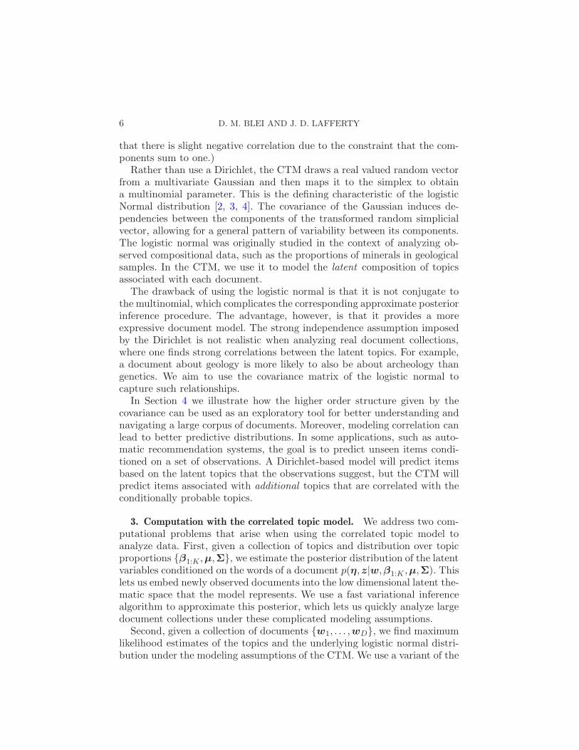
Rather than use a Dirichlet, the CTM draws a real valued random vectorfrom a multivariate Gaussian and then maps it to the simplex to obtaina multinomial parameter. This is the defining characteristic of the logisticNormal distribution [2, 3, 4]. The covariance of the Gaussian induces de-pendencies between the components of the transformed random simplicialvector, allowing for a general pattern of variability between its components.The logistic normal was originally studied in the context of analyzing ob-served compositional data, such as the proportions of minerals in geologicalsamples. In the CTM, we use it to model the latent composition of topicsassociated with each document.

The drawback of using the logistic normal is that it is not conjugate tothe multinomial, which complicates the corresponding approximate posteriorinference procedure. The advantage, however, is that it provides a moreexpressive document model. The strong independence assumption imposedby the Dirichlet is not realistic when analyzing real document collections,where one finds strong correlations between the latent topics. For example,a document about geology is more likely to also be about archeology thangenetics. We aim to use the covariance matrix of the logistic normal tocapture such relationships.

In Section 4 we illustrate how the higher order structure given by thecovariance can be used as an exploratory tool for better understanding andnavigating a large corpus of documents. Moreover, modeling correlation canlead to better predictive distributions. In some applications, such as auto-matic recommendation systems, the goal is to predict unseen items condi-tioned on a set of observations. A Dirichlet-based model will predict itemsbased on the latent topics that the observations suggest, but the CTM willpredict items associated with additional topics that are correlated with theconditionally probable topics.

3. Computation with the correlated topic model. We address two com-putational problems that arise when using the correlated topic model toanalyze data. First, given a collection of topics and distribution over topicproportions {β1:K ,µ,Σ}, we estimate the posterior distribution of the latentvariables conditioned on the words of a document p(η,z|w,β1:K ,µ,Σ). Thislets us embed newly observed documents into the low dimensional latent the-matic space that the model represents. We use a fast variational inferencealgorithm to approximate this posterior, which lets us quickly analyze largedocument collections under these complicated modeling assumptions.

Second, given a collection of documents {w1, . . . ,wD}, we find maximumlikelihood estimates of the topics and the underlying logistic normal distri-bution under the modeling assumptions of the CTM. We use a variant of the


expectation-maximization algorithm, where the E-step is the per-documentposterior inference problem described above. Furthermore, we seek sparsesolutions of the inverse covariance matrix between topics, and we adaptℓ1-regularized covariance estimation [20] for this purpose.

3.1. Posterior inference with variational methods. Given a document w

and a model {β1:K ,µ,Σ}, the posterior distribution of the per-documentlatent variables is

p(η,z|w,β1:K ,µ,Σ)(2)

=p(η|µ,Σ)

∏Nn=1 p(zn|η)p(wn|zn,β1:K)

∫p(η|µ,Σ)

∏Nn=1

∑Kzn=1 p(zn|η)p(wn|zn,β1:K)dη

,

which is intractable to compute due to the integral in the denominator, thatis, the marginal probability of the document that we are conditioning on.There are two reasons for this intractability. First, the sum over the K val-ues of zn occurs inside the product over words, inducing a combinatorialnumber of terms. Second, even if KN stays within the realm of compu-tational tractability, the distribution of topic proportions p(η|µ,Σ) is notconjugate to the distribution of topic assignments p(zn|η). Thus, we cannotanalytically compute the integrals of each term.

The nonconjugacy further precludes using many of the Monte Carlo Markovchain (MCMC) sampling techniques that have been developed for comput-ing with Dirichlet-based mixed membership models [10, 15]. These MCMCmethods are all based on Gibbs sampling, where the conjugacy between thelatent variables lets us compute coordinate-wise posteriors analytically. Toemploy MCMC in the logistic normal setting considered here, we have toappeal to a tailored Metropolis–Hastings solution. Such a technique will notenjoy the same convergence properties and speed of the Gibbs samplers,which is particularly hindering for the goal of analyzing collections thatcomprise millions of words.

Thus, to approximate this posterior, we appeal to variational methods asa deterministic alternative to MCMC. The idea behind variational methodsis to optimize the free parameters of a distribution over the latent variablesso that the distribution is close in Kullback–Leibler divergence to the trueposterior [17, 29]. The fitted variational distribution is then used as a substi-tute for the posterior, just as the empirical distribution of samples is used inMCMC. Variational methods have had widespread application in machinelearning; their potential in applied Bayesian statistics is beginning to berealized.

In models composed of conjugate-exponential family pairs and mixtures,the variational inference algorithm can be automatically derived by comput-ing expectations of natural parameters in the variational distribution [5, 7,


31]. However, the nonconjugate pair of variables in the CTM requires thatwe derive the variational inference algorithm from first principles.

We begin by using Jensen’s inequality to bound the log probability of adocument,

log p(w1:N |µ,Σ,β)

≥ Eq[log p(η|µ,Σ)] +N∑

n=1

Eq[log p(zn|η)](3)

+N∑

n=1

Eq[log p(wn|zn,β)] + H(q),

where the expectation is taken with respect to q, a variational distributionof the latent variables, and H(q) denotes the entropy of that distribution.As a variational distribution, we use a fully factorized model, where all thevariables are independently governed by a different distribution,

q(η1:K , z1:N |λ1:K , ν21:K ,φ1:N ) =

K∏

i=1

q(ηi|λi, ν2i )

N∏

n=1

q(zn|φn).(4)

The variational distributions of the discrete topic assignments z1:N are spec-ified by the K-dimensional multinomial parameters φ1:N (these are meanparameters of the multinomial). The variational distribution of the contin-uous variables η1:K are K independent univariate Gaussians {λi, νi}. Sincethe variational parameters are fit using a single observed document w1:N ,there is no advantage in introducing a nondiagonal variational covariancematrix.

The variational inference algorithm optimizes equation (3) with respectto the variational parameters, thereby tightening the bound on the marginalprobability of the observations as much as the structure of variational distri-bution allows. This is equivalent to finding the variational distribution thatminimizes KL(q||p), where p is the true posterior [17, 29]. Details of thisoptimization for the CTM are given in the Appendix.

Note that variational methods do not come with the same theoreticalguarantees as MCMC, where the limiting distribution of the chain is ex-actly the posterior of interest. However, variational methods provide fastalgorithms and a clear convergence criterion, whereas MCMC methods canbe computationally inefficient and determining when a Markov chain hasconverged is difficult [23].

3.2. Parameter estimation. Given a collection of documents, we carryout parameter estimation for the correlated topic model by attempting tomaximize the likelihood of a corpus of documents as a function of the topicsβ1:K and the multivariate Gaussian (µ,Σ).


As in many latent variable models, we cannot compute the marginal like-lihood of the data because of the latent structure that needs to be marginal-ized out. To address this issue, we use variational expectation–maximization(EM). In the E-step of traditional EM, one computes the posterior distri-bution of the latent variables given the data and current model parameters.In variational EM, we use the variational approximation to the posteriordescribed in the previous section. Note that this is akin to Monte Carlo EM,where the E-step is approximated by a Monte Carlo approximation to theposterior [30].

Specifically, the objective function of variational EM is the likelihoodbound given by summing equation (3) over the document collection {w1, . . . ,wD},

L(µ,Σ,β1:K ;w1:D) ≥D∑

d=1

Eqd[log p(ηd,zd,wd|µ,Σ,β1:K)] + H(qd).

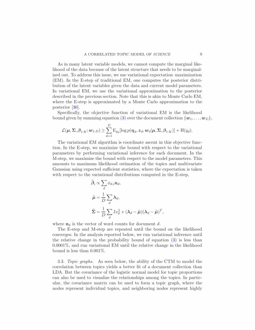
The variational EM algorithm is coordinate ascent in this objective func-tion. In the E-step, we maximize the bound with respect to the variationalparameters by performing variational inference for each document. In theM-step, we maximize the bound with respect to the model parameters. Thisamounts to maximum likelihood estimation of the topics and multivariateGaussian using expected sufficient statistics, where the expectation is takenwith respect to the variational distributions computed in the E-step,

βi ∝∑

d

φd,ind,

µ =1

D

∑

d

λd,

Σ =1

D

∑

d

Iν2d + (λd − µ)(λd − µ)T ,

where nd is the vector of word counts for document d.The E-step and M-step are repeated until the bound on the likelihood

converges. In the analysis reported below, we run variational inference untilthe relative change in the probability bound of equation (3) is less than0.0001%, and run variational EM until the relative change in the likelihoodbound is less than 0.001%.

3.3. Topic graphs. As seen below, the ability of the CTM to model thecorrelation between topics yields a better fit of a document collection thanLDA. But the covariance of the logistic normal model for topic proportionscan also be used to visualize the relationships among the topics. In partic-ular, the covariance matrix can be used to form a topic graph, where thenodes represent individual topics, and neighboring nodes represent highly


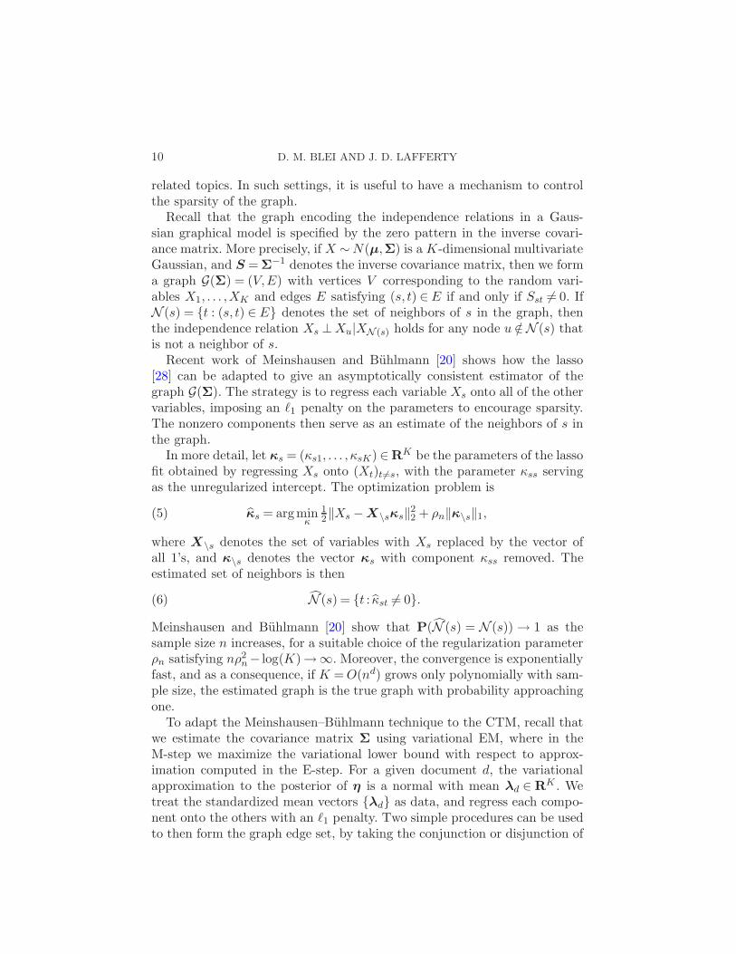
related topics. In such settings, it is useful to have a mechanism to controlthe sparsity of the graph.

Recall that the graph encoding the independence relations in a Gaus-sian graphical model is specified by the zero pattern in the inverse covari-ance matrix. More precisely, if X ∼ N(µ,Σ) is a K-dimensional multivariateGaussian, and S = Σ

−1 denotes the inverse covariance matrix, then we forma graph G(Σ) = (V,E) with vertices V corresponding to the random vari-ables X1, . . . ,XK and edges E satisfying (s, t) ∈ E if and only if Sst 6= 0. IfN (s) = {t : (s, t) ∈ E} denotes the set of neighbors of s in the graph, thenthe independence relation Xs ⊥ Xu|XN (s) holds for any node u /∈N (s) thatis not a neighbor of s.

Recent work of Meinshausen and Buhlmann [20] shows how the lasso[28] can be adapted to give an asymptotically consistent estimator of thegraph G(Σ). The strategy is to regress each variable Xs onto all of the othervariables, imposing an ℓ1 penalty on the parameters to encourage sparsity.The nonzero components then serve as an estimate of the neighbors of s inthe graph.

In more detail, let κs = (κs1, . . . , κsK) ∈RK be the parameters of the lasso

fit obtained by regressing Xs onto (Xt)t6=s, with the parameter κss servingas the unregularized intercept. The optimization problem is

κs = argminκ

12‖Xs −X\sκs‖

22 + ρn‖κ\s‖1,(5)

where X\s denotes the set of variables with Xs replaced by the vector ofall 1’s, and κ\s denotes the vector κs with component κss removed. Theestimated set of neighbors is then

N (s) = {t : κst 6= 0}.(6)

Meinshausen and Buhlmann [20] show that P(N (s) = N (s)) → 1 as thesample size n increases, for a suitable choice of the regularization parameterρn satisfying nρ2

n− log(K)→∞. Moreover, the convergence is exponentiallyfast, and as a consequence, if K = O(nd) grows only polynomially with sam-ple size, the estimated graph is the true graph with probability approachingone.

To adapt the Meinshausen–Buhlmann technique to the CTM, recall thatwe estimate the covariance matrix Σ using variational EM, where in theM-step we maximize the variational lower bound with respect to approx-imation computed in the E-step. For a given document d, the variationalapproximation to the posterior of η is a normal with mean λd ∈ R

K . Wetreat the standardized mean vectors {λd} as data, and regress each compo-nent onto the others with an ℓ1 penalty. Two simple procedures can be usedto then form the graph edge set, by taking the conjunction or disjunction of


the local neighborhood estimates:

(s, t) ∈ EAND in case t ∈ N (s) and s ∈ N (t),(7)

(s, t) ∈ EOR in case t ∈ N (s) or s ∈ N (t).(8)

Figure 2 shows an example of a topic graph constructed using this method,with edges EAND formed by intersecting the neighborhood estimates. Vary-ing the regularization parameter ρn allows control over the sparsity of thegraph; the graph becomes increasingly sparse as ρn increases.

4. Analyzing Science. JSTOR is an on-line archive of scholarly journalsthat scans bound volumes dating back to the 1600s and runs optical char-acter recognition algorithms on the scans. Thus, JSTOR stores and indexeshundreds of millions of pages of noisy text, all searchable through the Inter-net. This is an invaluable resource to scholars.

The JSTOR collection provides an opportunity for developing exploratoryanalysis and useful descriptive statistics of large volumes of text data. Asthey are, the articles are organized by journal, volume and number. Butthe users of JSTOR would benefit from a topical organization of articlesfrom different journals and automatic recommendations of similar articlesto those known to be of interest.

In some modern electronic scholarly archives, such as the ArXiv(http://www.arxiv.org/), contributors provide meta-data with their manu-scripts that describe and categorize their work to aid in such a topical ex-ploration of the collection. In many text data sets, however, meta-data isunavailable. Moreover, there may be underlying topics and connections be-tween articles that the authors or curators have not determined. To theseends, we analyzed a large portion of JSTOR’s corpus of articles from Science

with the CTM.

4.1. Qualitative analysis of Science. In this section we illustrate the pos-sible applications of the CTM to automatic corpus analysis and browsing.We estimated a 100-topic model on the Science articles from 1990 to 1999using the variational EM algorithm of Section 3.2. (C code that implementsthis algorithm can be found at the first author’s web-site and STATLIB.)The total vocabulary size in this collection is 375,144 terms. We trim the356,195 terms that occurred fewer than 70 times as well as 296 stop words,that is, words like “the,” “but” or “with,” which do not convey meaning.This yields a corpus of 16,351 documents, 19,088 unique terms and a totalof 5.7M words.

Using the technique described in Section 3.3, we constructed a sparsegraph (ρ = 0.1) of the connections between the estimated latent topics. Partof this graph is illustrated in Figure 2. (For space, we manually removed

http://www.arxiv.org/

12

D.M

.B

LE

IA

ND

J.D

.LA

FFE

RT

Y

Fig. 2. A portion of the topic graph learned from 16,351 OCR articles from Science (1990–1999). Each topic node is labeled with itsfive most probable phrases and has font proportional to its popularity in the corpus. (Phrases are found by permutation test.) The fullmodel can be found in http://www.cs.cmu.edu/˜lemur/science/ and on STATLIB.

http://www.cs.cmu.edu/~lemur/science/


topics that occurred very rarely and those that captured nontopical contentsuch as front matter.) This graph provides a snapshot of ten years of Sci-

ence, and reveals different substructures of themes in the collection. A userinterested in the brain can restrict attention to articles that use the neuro-science topics; a user interested in genetics can restrict attention to thosearticles in the cluster of genetics topics.

Further structure is revealed at the document level, where each documentis associated with a latent vector of topic proportions. The posterior distri-bution of the proportions can be used to associate documents with latenttopics. For example, the following are the top five articles associated withthe topic whose most probable vocabulary items are “laser, optical, light,electron, quantum”:

1. “Vacuum Squeezing of Solids: Macroscopic Quantum States Driven byLight Pulses” (1997).

2. “Superradiant Rayleigh Scattering from a Bose–Einstein Condensate”(1999).

3. “Physics and Device Applications of Optical Microcavities” (1992).4. “Photon Number Squeezed States in Semiconductor Lasers” (1992).5. “A Well-Collimated Quasi-Continuous Atom Laser” (1999).

Moreover, we can use the expected distance between per-document topicproportions to identify other documents that have similar topical content.We use the expected Hellinger distance, which is a symmetric distance be-tween distributions. Consider two documents i and j,

E[d(θi,θj)] = Eq

[∑

k

(√

θik −√

θjk)2

]

= 2− 2∑

k

Eq[√

θik]Eq

[θjk√θjk

],

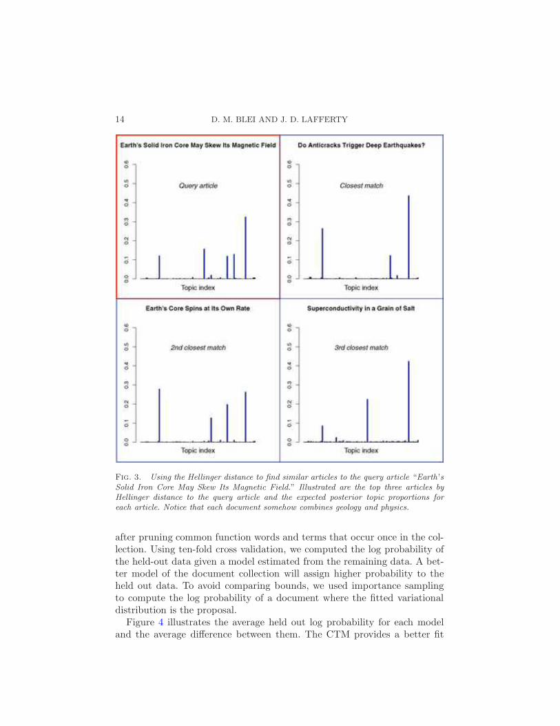
where all expectations are taken with respect to the variational posteriordistributions (see Section 3.1). One example of this application of the latentvariable analysis is illustrated in Figure 3.

The interested reader is invited to visit http://www.cs.cmu.edu/∼lemur/science/to interactively explore this model, including the topics, their connections,the articles that exhibit them and the expected Hellinger similarity betweenarticles.

4.2. Quantitative comparison to latent Dirichlet allocation. We comparedthe logistic normal to the Dirichlet by fitting a smaller collection of articlesto CTM and LDA models of varying numbers of topics. This collection con-tains the 1,452 documents from 1960; we used a vocabulary of 5,612 words

http://www.cs.cmu.edu/~lemur/science/


Fig. 3. Using the Hellinger distance to find similar articles to the query article “Earth’sSolid Iron Core May Skew Its Magnetic Field.” Illustrated are the top three articles byHellinger distance to the query article and the expected posterior topic proportions foreach article. Notice that each document somehow combines geology and physics.

after pruning common function words and terms that occur once in the col-lection. Using ten-fold cross validation, we computed the log probability ofthe held-out data given a model estimated from the remaining data. A bet-ter model of the document collection will assign higher probability to theheld out data. To avoid comparing bounds, we used importance samplingto compute the log probability of a document where the fitted variationaldistribution is the proposal.

Figure 4 illustrates the average held out log probability for each modeland the average difference between them. The CTM provides a better fit


Fig. 4. (Left) The 10-fold cross-validated held-out log probability of the 1960 Sciencecorpus, computed by importance sampling. The CTM supports more topics than LDA. Seefigure at right for the standard error of the difference. (Right) The mean difference inheld-out log probability. Numbers greater than zero indicate a better fit by the CTM.

than LDA and supports more topics; the likelihood for LDA peaks near 30topics, while the likelihood for the CTM peaks close to 90 topics. The meansand standard errors of the difference in log-likelihood of the models is shownat right; this indicates that the CTM always gives a better fit.

Another quantitative evaluation of the relative strengths of LDA and theCTM is how well the models predict the remaining words of a document afterobserving a portion of it. Specifically, we observe P words from a documentand are interested in which model provides a better predictive distributionof the remaining words p(w|w1:P ). To compare these distributions, we useperplexity, which can be thought of as the effective number of equally likelywords according to the model. Mathematically, the perplexity of a worddistribution is defined as the inverse of the per-word geometric average ofthe probability of the observations,

Perp(Φ) =

(D∏

d=1

Nd∏

i=P+1

p(wi|Φ,w1:P )

)−1/(∑D

d=1(Nd−P ))

,

where Φ denotes the model parameters of an LDA or CTM model. Notethat lower numbers denote more predictive power.

The plot in Figure 5 compares the predictive perplexity under LDA andthe CTM for different numbers of words randomly observed from the doc-uments. When a small number of words have been observed, there is lessuncertainty about the remaining words under the CTM than under LDA—the perplexity is reduced by nearly 200 words, or roughly 10%. The reason


Fig. 5. (Left) The 10-fold cross-validated predictive perplexity for partially observedheld-out documents from the 1960 Science corpus (K = 50). Lower numbers indicate morepredictive power from the CTM. (Right) The mean difference in predictive perplexity.Numbers less than zero indicate better prediction from the CTM.

is that after seeing a few words in one topic, the CTM uses topic correlationto infer that words in a related topic may also be probable. In contrast,LDA cannot predict the remaining words as well until a large portion of thedocument has been observed so that all of its topics are represented.

5. Summary. We have developed a hierarchical topic model of docu-ments that replaces the Dirichlet distribution of per-document topic pro-portions with a logistic normal. This allows the model to capture correla-tions between the occurrence of latent topics. The resulting correlated topicmodel gives better predictive performance and uncovers interesting descrip-tive statistics for facilitating browsing and search. Use of the logistic normal,while more complex, may have benefit in the many applications of Dirichlet-based mixed membership models.

One issue that we did not thoroughly explore is model selection, that is,choosing the number of topics for a collection. In other topic models, non-parametric Bayesian methods based on the Dirichlet process are a naturalsuite of tools because they can accommodate new topics as more documentsare observed. (The nonparametric Bayesian version of LDA is exactly thehierarchical Dirichlet process [27].) The logistic normal, however, does notimmediately give way to such extensions. Tackling the model selection issuein this setting is an important area of future research.

APPENDIX: DETAILS OF VARIATIONAL INFERENCE

Variational objective. Before deriving the optimization procedure, we


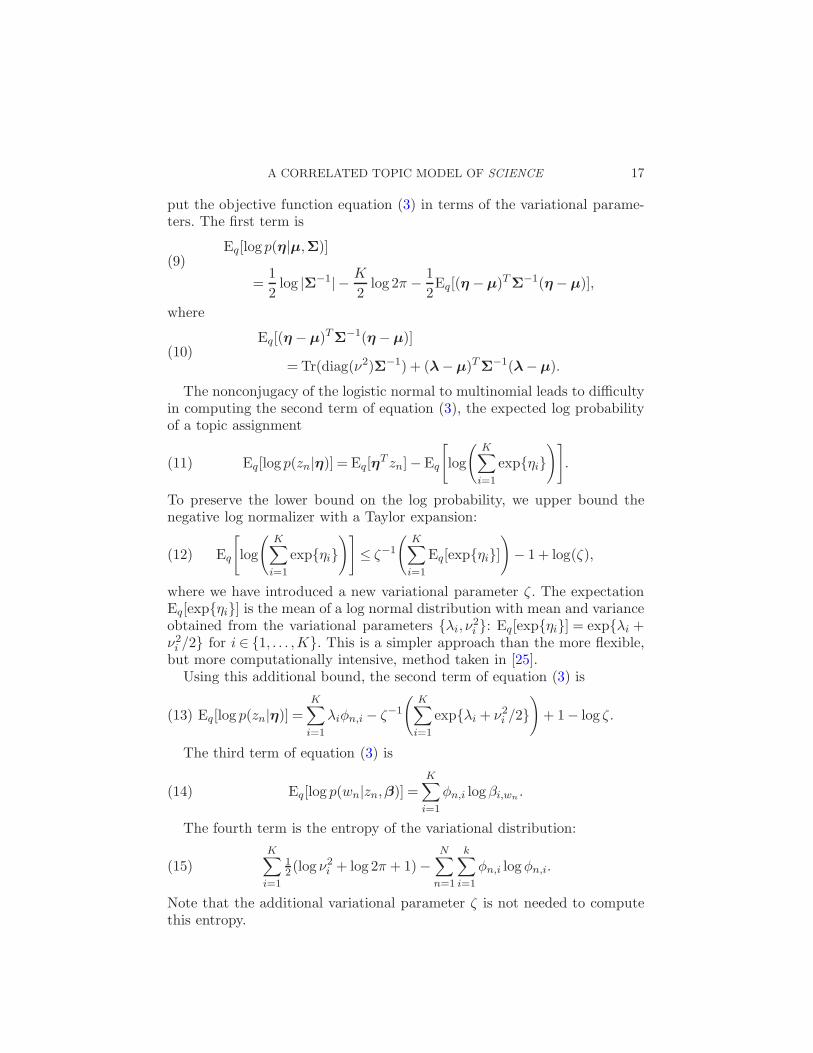
put the objective function equation (3) in terms of the variational parame-ters. The first term is

Eq[log p(η|µ,Σ)](9)

=1

2log |Σ−1| −

K

2log 2π −

1

2Eq[(η −µ)T Σ

−1(η −µ)],

where

Eq[(η −µ)TΣ−1(η −µ)]

(10)= Tr(diag(ν2)Σ−1) + (λ−µ)T Σ

−1(λ−µ).

The nonconjugacy of the logistic normal to multinomial leads to difficultyin computing the second term of equation (3), the expected log probabilityof a topic assignment

Eq[log p(zn|η)] = Eq[ηT zn]−Eq

[log

(K∑

i=1

exp{ηi}

)].(11)

To preserve the lower bound on the log probability, we upper bound thenegative log normalizer with a Taylor expansion:

Eq

[log

(K∑

i=1

exp{ηi}

)]≤ ζ−1

(K∑

i=1

Eq[exp{ηi}]

)− 1 + log(ζ),(12)

where we have introduced a new variational parameter ζ . The expectationEq[exp{ηi}] is the mean of a log normal distribution with mean and varianceobtained from the variational parameters {λi, ν

2i }: Eq[exp{ηi}] = exp{λi +

ν2i /2} for i ∈ {1, . . . ,K}. This is a simpler approach than the more flexible,

but more computationally intensive, method taken in [25].Using this additional bound, the second term of equation (3) is

Eq[log p(zn|η)] =K∑

i=1

λiφn,i − ζ−1

(K∑

i=1

exp{λi + ν2i /2}

)+ 1− log ζ.(13)

The third term of equation (3) is

Eq[log p(wn|zn,β)] =K∑

i=1

φn,i logβi,wn .(14)

The fourth term is the entropy of the variational distribution:

K∑

i=1

12 (log ν2

i + log 2π + 1)−N∑

n=1

k∑

i=1

φn,i logφn,i.(15)

Note that the additional variational parameter ζ is not needed to computethis entropy.


Coordinate ascent optimization. Finally, we maximize the bound in equa-tion (3) with respect to the variational parameters λ1:K , ν1:K , φ1:N and ζ .We use a coordinate ascent algorithm, iteratively maximizing the boundwith respect to each parameter.

First, we maximize equation (3) with respect to ζ , using the second boundin equation (12). The derivative with respect to ζ is

f ′(ζ) = N

(ζ−2

(K∑

i=1

exp{λi + ν2i /2}

)− ζ−1

),(16)

which has a maximum at

ζ =K∑

i=1

exp{λi + ν2i /2}.(17)

Second, we maximize with respect to φn. This yields a maximum at

φn,i ∝ exp{λi}βi,wn , i ∈ {1, . . . ,K},(18)

which is an application of variational inference updates within the exponen-tial family [5, 7, 31].

Third, we maximize with respect to λi. Equation (3) is not amenableto analytic maximization. We use the conjugate gradient algorithm withderivative

dL/dλ =−Σ−1(λ−µ) +

N∑

n=1

φn,1:K − (N/ζ) exp{λ + ν2/2}.(19)

Finally, we maximize with respect to ν2i . Again, there is no analytic solution.

We use Newton’s method for each coordinate with the constraint that νi > 0,

dL/dν2i =−Σ

−1ii /2−N/2ζ exp{λi + ν2

i /2}+ 1/(2ν2i ).(20)

Iterating between the optimizations of ν, λ, φ and ζ defines a coordinateascent algorithm on equation (3). (In practice, we optimize with respectto ζ in between optimizations for ν, λ and φ.) Though each coordinate’soptimization is convex, the variational objective is not convex with respectto the ensemble of variational parameters. We are only guaranteed to find alocal maximum, but note that this is still a bound on the log probability ofa document.

Acknowledgments. We thank two anonymous reviewers for their excel-lent suggestions for improving the paper. We thank JSTOR for providingaccess to journal material in the JSTOR archive. We thank Jon McAuliffeand Nathan Srebro for useful discussions and comments. A preliminary ver-sion of this work appears in [9].


REFERENCES

[1] Airoldi, E., Blei, D., Fienberg, S. and Xing, E. (2007). Combining stochasticblock models and mixed membership for statistical network analysis. StatisticalNetwork Analysis: Models, Issues and New Directions. Lecture Notes in Comput.Sci. 4503 57–74. Springer, Berlin.

[2] Aitchison, J. (1982). The statistical analysis of compositional data (with discus-sion). J. Roy. Statist. Soc. Ser. B 44 139–177. MR0676206

[3] Aitchison, J. (1985). A general class of distributions on the simplex. J. Roy. Statist.Soc. Ser. B 47 136–146. MR0805071

[4] Aitchison, J. and Shen, S. (1980). Logistic normal distributions: Some propertiesand uses. Biometrika 67 261–272. MR0581723

[5] Bishop, C., Spiegelhalter, D. and Winn, J. (2003). VIBES: A variational infer-ence engine for Bayesian networks. In Advances in Neural Information Process-ing Systems 15 (S. Becker, S. Thrun and K. Obermayer, eds.) 777–784. MITPress, Cambridge, MA. MR2003168

[6] Blei, D. and Jordan, M. (2003). Modeling annotated data. In Proceedings of the26th annual International ACM SIGIR Conference on Research and Develop-ment in Information Retrieval 127–134. ACM Press, New York, NY.

[7] Blei, D. and Jordan, M. (2005). Variational inference for Dirichlet process mixtures.Journal of Bayesian Analysis 1 121–144. MR2227367

[8] Blei, D., Ng, A. and Jordan, M. (2003). Latent Dirichlet allocation. Journal ofMachine Learning Research 3 993–1022.

[9] Blei, D. M. and Lafferty, J. D. (2006). Correlated topic models. In Advances inNeural Information Processing Systems 18 (Y. Weiss, B. Scholkopf and J. Platt,eds.). MIT Press, Cambridge, MA.

[10] Erosheva, E. (2002). Grade of membership and latent structure models with appli-cation to disability survey data. Ph.D. thesis, Dept. Statistics, Carnegie MellonUniv.

[11] Erosheva, E., Fienberg, S. and Joutard, C. (2007). Describing disability throughindividual-level mixture models for multivariate binary data. Ann. Appl. Statist.To appear.

[12] Erosheva, E., Fienberg, S. and Lafferty, J. (2004). Mixed-membership modelsof scientific publications. Proc. Natl. Acad. Sci. USA 97 11885–11892.

[13] Fei-Fei, L. and Perona, P. (2005). A Bayesian hierarchical model for learningnatural scene categories. IEEE Computer Vision and Pattern Recognition 2 524–531.

[14] Girolami, M. and Kaban, A. (2004). Simplicial mixtures of Markov chains: Dis-tributed modelling of dynamic user profiles. In Advances in Neural InformationProcesing Systems 16 9–16. MIT Press, Cambridge, MA.

[15] Griffiths, T. and Steyvers, M. (2004). Finding scientific topics. Proc. Natl. Acad.Sci. USA 101 5228–5235.

[16] Griffiths, T., Steyvers, M., Blei, D. and Tenenbaum, J. (2005). Integratingtopics and syntax. In Advances in Neural Information Processing Systems 17

537–544. MIT Press, Cambridge, MA.[17] Jordan, M., Ghahramani, Z., Jaakkola, T. and Saul, L. (1999). Introduction

to variational methods for graphical models. Machine Learning 37 183–233.[18] Marlin, B. (2004). Collaborative filtering: A machine learning perspective. Master’s

thesis, Univ. Toronto.[19] McCallum, A., Corrada-Emmanuel, A. and Wang, X. (2004). The author–

recipient–topic model for topic and role discovery in social networks: Experi-

http://www.ams.org/mathscinet-getitem?mr=0676206






ments with Enron and academic email. Technical report, Univ. Massachusetts,Amherst.

[20] Meinshausen, N. and Buhlmann, P. (2006). High dimensional graphs and variableselection with the lasso. Ann. Statist. 34 1436–1462. MR2278363

[21] Mosteller, F. and Wallace, D. L. (1964). Inference and Disputed Authorship:The Federalist. Addison-Wesley, Reading, MA. MR0175668

[22] Pritchard, J., Stephens, M. and Donnelly, P. (2000). Inference of populationstructure using multilocus genotype data. Genetics 155 945–959.

[23] Robert, C. and Casella, G. (2004). Monte Carlo Statistical Methods, 2nd ed.Springer, New York. MR2080278

[24] Rosen-Zvi, M., Griffiths, T., Steyvers, M. and Smith, P. (2004). The author-topic model for authors and documents. In AUAI ’04 : Proceedings of the 20thConference on Uncertainty in Artificial Intelligence 487–494. AUAI Press, Ar-lington, VA.

[25] Saul, L., Jaakkola, T. and Jordan, M. (1996). Mean field theory for sigmoidbelief networks. Journal of Artificial Intelligence Research 4 61–76.

[26] Sivic, J., Rusell, B., Efros, A., Zisserman, A. and Freeman, W. (2005). Dis-covering object categories in image collections. Technical report, CSAIL, Mas-sachusetts Institute of Technology.

[27] Teh, Y., Jordan, M., Beal, M. and Blei, D. (2007). Hierarchical Dirichlet pro-cesses. J. Amer. Statist. Assoc. 101 1566–1581.

[28] Tibshirani, R. (1996). Regression shrinkage and selection via the lasso. J. R. Statist.Soc. Ser. B Stat. Methodol. 58 267–288. MR1379242

[29] Wainwright, M. and Jordan, M. (2003). Graphical models, exponential families,and variational inference. Technical Report 649, Dept. Statistics, U.C. Berkeley.

[30] Wei, G. and Tanner, M. (1990). A Monte Carlo implementation of the EM al-gorithm and the poor man’s data augmentation algorithms. J. Amer. Statist.Assoc. 85 699–704.

[31] Xing, E., Jordan, M. and Russell, S. (2003). A generalized mean field algorithmfor variational inference in exponential families. In Proceedings of UAI 583–591.Morgan Kaufmann, San Francisco, CA.

Computer Science Department

Princeton University

Princeton, New Jersey 08540

USA

E-mail: [email protected]

Computer Science Department

Machine Learning Department

Carnegie Mellon University

Pittsburgh, Pennsylvania 15213

USA

E-mail: [email protected]





mailto:[email protected]

mailto:[email protected]

A correlated topic model of SCIENCE - arXiv

Documents

Transcript of A correlated topic model of SCIENCE - arXiv