A Computer Tool for Modelling CO2 Emissions in Driving ...
33
energies Article A Computer Tool for Modelling CO 2 Emissions in Driving Cycles for Spark Ignition Engines Powered by Biofuels Karol Tucki Citation: Tucki, K. A Computer Tool for Modelling CO 2 Emissions in Driving Cycles for Spark Ignition Engines Powered by Biofuels. Energies 2021, 14, 1400. https://doi.org/ 10.3390/en14051400 Academic Editor: Constantine D. Rakopoulos Received: 9 February 2021 Accepted: 1 March 2021 Published: 4 March 2021 Publisher’s Note: MDPI stays neutral with regard to jurisdictional claims in published maps and institutional affil- iations. Copyright: © 2021 by the author. Licensee MDPI, Basel, Switzerland. This article is an open access article distributed under the terms and conditions of the Creative Commons Attribution (CC BY) license (https:// creativecommons.org/licenses/by/ 4.0/). Department of Production Engineering, Institute of Mechanical Engineering, Warsaw University of Life Sciences, Nowoursynowska Street 164, 02-787 Warsaw, Poland; [email protected]; Tel.: +48-593-45-78 Abstract: A driving cycle is a record intended to reflect the regular use of a given type of vehicle, presented as a speed profile recorded over a certain period of time. It is used for the assessment of engine pollutant emissions, fuel consumption analysis and environmental certification procedures. Different driving cycles are used, depending on the region of the world. In addition, drive cycles are used by car manufacturers to optimize vehicle drivelines. The basis of the work presented in the manuscript was a developed computer tool using tests on the Toyota Camry LE 2018 chassis dy- namometer, the results of the optimization process of neural network structures and the properties of fuels and biofuels. As a result of the work of the computer tool, the consumption of petrol 95, ethanol, methanol, DME, CNG, LPG and CO 2 emissions for the vehicle in question were analyzed in the fol- lowing driving tests: Environmental Protection Agency (EPA US06 and EPA USSC03); Supplemental Federal Test Procedure (SFTP); Highway Fuel Economy Driving Schedule (HWFET); Federal Test Procedure (FTP-75–EPA); New European Driving Cycle (NEDC); Random Cycle Low (×05); Random Cycle High (×95); Mobile Air Conditioning Test Procedure (MAC TP); Common Artemis Driving Cycles (CADC–Artemis); Worldwide Harmonized Light-Duty Vehicle Test Procedure (WLTP). Keywords: car; fuel; biofuel; neural model 1. Introduction The dynamic development of technology, which the automotive industry has seen for many years, includes both achieving an appropriate level of vehicle performance and meeting appropriate environmental protection requirements [1–4]. Keeping exhaust gas emissions under the permissible limits is the basic criterion that determines the directions of further development of engines used to drive motor vehicles [5–8]. Increasingly restrictive legal regulations are introduced to protect the climate [9–12]. The European Union (EU) has long been setting ambitious climate goals, which will not be achievable without reducing greenhouse gas emissions in transport—which consumes a third of the energy in the EU [13–15]. It is the transport sector in the EU that accounts for almost 30% of total CO 2 emissions, 72% of which comes from road transport [16,17]. Passenger cars are responsible for 60.7% of all CO 2 emissions from road transport in Europe [18,19]. Additionally, in the United States, car exhaust gases are the main source of greenhouse gas emissions, thus causing climate change [20–22]. The local permissible exhaust emission standards are based on research by a federal US body—the Environmental Protection Agency (EPA) [23,24]. Greenhouse gas emissions from transport account for approximately 28 percent of total US greenhouse gas emissions [25,26]. In China, combustion tests are a mixture of the abovementioned European and Ameri- can regulations [27,28]. Work is also underway on a new type of test, which will be even more complicated and will much better reflect actual conditions [29,30]. The Chinese transport sector is responsible for around 12% of domestic emissions [31–34]. Each new passenger car must meet exhaust gas toxicity standards before it is intro- duced to the market [35–37]. The test conditions depend on the vehicle class and the Energies 2021, 14, 1400. https://doi.org/10.3390/en14051400 https://www.mdpi.com/journal/energies
-
Upload
khangminh22 -
Category
Documents
-
view
1 -
download
0
Transcript of A Computer Tool for Modelling CO2 Emissions in Driving ...
energies
Article
A Computer Tool for Modelling CO2 Emissions in DrivingCycles for Spark Ignition Engines Powered by Biofuels
Karol Tucki
�����������������
Citation: Tucki, K. A Computer Tool
for Modelling CO2 Emissions in
Driving Cycles for Spark Ignition
Engines Powered by Biofuels. Energies
2021, 14, 1400. https://doi.org/
10.3390/en14051400
Academic Editor: Constantine
D. Rakopoulos
Received: 9 February 2021
Accepted: 1 March 2021
Published: 4 March 2021
Publisher’s Note: MDPI stays neutral
with regard to jurisdictional claims in
published maps and institutional affil-
iations.
Copyright: © 2021 by the author.
Licensee MDPI, Basel, Switzerland.
This article is an open access article
distributed under the terms and
conditions of the Creative Commons
Attribution (CC BY) license (https://
creativecommons.org/licenses/by/
4.0/).
Department of Production Engineering, Institute of Mechanical Engineering, Warsaw University of Life Sciences,Nowoursynowska Street 164, 02-787 Warsaw, Poland; [email protected]; Tel.: +48-593-45-78
Abstract: A driving cycle is a record intended to reflect the regular use of a given type of vehicle,presented as a speed profile recorded over a certain period of time. It is used for the assessment ofengine pollutant emissions, fuel consumption analysis and environmental certification procedures.Different driving cycles are used, depending on the region of the world. In addition, drive cyclesare used by car manufacturers to optimize vehicle drivelines. The basis of the work presented inthe manuscript was a developed computer tool using tests on the Toyota Camry LE 2018 chassis dy-namometer, the results of the optimization process of neural network structures and the properties offuels and biofuels. As a result of the work of the computer tool, the consumption of petrol 95, ethanol,methanol, DME, CNG, LPG and CO2 emissions for the vehicle in question were analyzed in the fol-lowing driving tests: Environmental Protection Agency (EPA US06 and EPA USSC03); SupplementalFederal Test Procedure (SFTP); Highway Fuel Economy Driving Schedule (HWFET); Federal TestProcedure (FTP-75–EPA); New European Driving Cycle (NEDC); Random Cycle Low (×05); RandomCycle High (×95); Mobile Air Conditioning Test Procedure (MAC TP); Common Artemis DrivingCycles (CADC–Artemis); Worldwide Harmonized Light-Duty Vehicle Test Procedure (WLTP).
Keywords: car; fuel; biofuel; neural model
1. Introduction
The dynamic development of technology, which the automotive industry has seenfor many years, includes both achieving an appropriate level of vehicle performance andmeeting appropriate environmental protection requirements [1–4]. Keeping exhaust gasemissions under the permissible limits is the basic criterion that determines the directions offurther development of engines used to drive motor vehicles [5–8]. Increasingly restrictivelegal regulations are introduced to protect the climate [9–12]. The European Union (EU) haslong been setting ambitious climate goals, which will not be achievable without reducinggreenhouse gas emissions in transport—which consumes a third of the energy in theEU [13–15]. It is the transport sector in the EU that accounts for almost 30% of total CO2emissions, 72% of which comes from road transport [16,17]. Passenger cars are responsiblefor 60.7% of all CO2 emissions from road transport in Europe [18,19].
Additionally, in the United States, car exhaust gases are the main source of greenhousegas emissions, thus causing climate change [20–22]. The local permissible exhaust emissionstandards are based on research by a federal US body—the Environmental ProtectionAgency (EPA) [23,24]. Greenhouse gas emissions from transport account for approximately28 percent of total US greenhouse gas emissions [25,26].
In China, combustion tests are a mixture of the abovementioned European and Ameri-can regulations [27,28]. Work is also underway on a new type of test, which will be evenmore complicated and will much better reflect actual conditions [29,30]. The Chinesetransport sector is responsible for around 12% of domestic emissions [31–34].
Each new passenger car must meet exhaust gas toxicity standards before it is intro-duced to the market [35–37]. The test conditions depend on the vehicle class and the
Energies 2021, 14, 1400. https://doi.org/10.3390/en14051400 https://www.mdpi.com/journal/energies
Energies 2021, 14, 1400 2 of 33
country of destination [38–40]. Such tests, carried out in laboratory conditions, enable therepeatability and comparability of the obtained results [41–43]. By carrying out such tests,it is possible to avoid many of the risk factors associated with the actual road testing of vehi-cles that will affect fuel consumption—such as driving style, terrain or weather conditions.In order to execute these tests, a chassis dynamometer is needed (on a roller dynamometricstand) with adjustable motion resistance and execution of driving cycles [44–46].
Until August 2017, light vehicles in the European Union (with a reference mass notexceeding 2610 kg) were tested with the standard New European Driving Cycle (NEDC)driving test that included four repeated Urban Driving Cycles (UDCs) and one Extra UrbanDriving Cycle (EUDC) [47–50]. Since September 2017, there has been a new procedure inforce in the EU in the area of fuel consumption, carbon dioxide and exhaust emission stan-dards: the Worldwide Harmonized Light-Duty Vehicles Test Procedure (WLTP) EU [51–53].Although the WLTP is also a test carried out under laboratory conditions, it covers situ-ations possibly closest to everyday actual operating conditions. Four speed ranges aremeasured from the moment the engine is started: up to 60, up to 80, up to 100 and over130 km/h. During each of these phases, the vehicle always slows down and acceler-ates [54,55]. The maximum speed is 10 km/h more than that of the NEDC test. The averagespeed is 47 km/h—much higher than the previous 33 km/h. A complete WLTP cycle takesabout 30 min, whereas the NEDC only takes about 20 min [56–58]. The cycle distance hasmore than doubled and is now 23 km instead of the previous 11 km. Unlike the NEDCcycle, the requirements of the car’s electrical system and additional equipment are alsotaken into account: its weight, aerodynamics and rolling resistance [59,60]. Any additionalvehicle equipment that is highly energy-consuming, such as those with air conditioning orheated seats, remains excluded from the WLTP test [61,62].
The conditions for dynamometric testing and vehicle loading are based on the strictguidelines of the WLTP test procedure including several Worldwide Harmonized Light-Duty Vehicles Test Cycles (WLTC) [63,64]. These cycles are applicable to vehicle categorieswith different power-to-weight ratios (unladen weight) [65,66].
In addition to the WLTP, the EU Commission also enforces the so-called Real DrivingEmissions (RDE) as an additional approval requirement under Article EU6d of the directivefor emissions [67–70]. Contrary to the NEDC and WLTP, the RDE tests set out acceptablelimits for nitrogen oxides (NOx) and solid particle emissions in real conditions [71,72].The RDE does not require a strictly defined driving cycle. Its parameters, including distance,acceleration, outside temperature, wind strength or traffic intensity, are freely selectedwithin the specified statistical boundary conditions [73–75].
The European project Assessment and Reliability of Transport Emission Models andInventory Systems (ARTEMIS) developed a chassis dynamometer procedure called Com-mon Artemis Driving Cycles (CADC) that can be characterized by stronger acceleration,higher driving dynamics and a realistic proportion of high speeds (with peaks up to 130and 150 km/h) [76–78]. The cycles realized as part of the procedure include three drivingplans: urban (distance 4.8 km), rural road (distance 17.2 km) and two variants of themotorway plan (distances of 28.7 and 29.5 km) [79–81].
There is a test procedure in the EU for measuring additional fuel consumption andpollutant emissions caused by the operation of the Mobile Air Conditioning (MAC) systemin a passenger car [82–84]. The procedure for a physical test of the whole vehicle on achassis dynamometer includes a double test run (with MAC ON and MAC OFF) with thesame three phases of the fixed condition of the test cycle [85,86].
In the United States of America, the Federal Transient Procedure (FTP-75) test is usedto evaluate the environmental performance of passenger cars and delivery vans, whereasthe Highway Federal Extra Test (HWFET) test is used to assess fuel consumption [87–90].The FTP-75 simulates a city route with frequent stops, combined with both a cold andhot start transition phase [91–93]. The entire cycle, in which the vehicle travels 17.77 km,at an average speed of 34.12 km/h, takes about 31 min [94,95]. Cycle FTP-75 is among twovariants of the Urban Dynamometer Driving Schedule (UDDS).

Energies 2021, 14, 1400 3 of 33
Furthermore, the Supplemental Federal Test Procedure (SFTP) applies [96,97]. It wasdeveloped for the purposes of a driving analysis of a vehicle with an air conditioner,dynamic changes in its driving speed as well as acceleration and deceleration of the vehicle.The high speed and rapid acceleration analysis was covered by the US06 SFTP cycle andstandards [98–101]. During the cycle, the car covers a distance of 12.8 km in 596 s, reachinga maximum speed of 129.2 km/h [102,103]. An additional SC03 SFTP test procedure coversan analysis of emissions related to the use of air conditioners on vehicles certified underthe FTP-75 test cycle [104–106]. In this test, the vehicle travels 5.8 km in 596 s, reaching amaximum speed of 88.2 km/h [107,108]. It should be emphasized that the SFTP emissionlevels are a combination of the emission levels of the two test cycles and the FTP cycle.This means that the SFTP emissions from each test group of vehicles must meet all SFTP andFTP emission standards [109]. In addition, there is the California Unified Cycle LA92 [110].
The diminishing resources of natural fossil fuels and the growing demand for energypose serious social, technological and scientific challenges [111–115]. Alternative fuelshave been developed for many years, and their use in the automotive industry will un-doubtedly continue to be verified in the context of road tests [116–120]. Alternative fuelsfor internal combustion engines are defined in relation to the classic liquid petroleumfuels, such as petrol for spark ignition engines and diesel oil for compression ignitionengines [121–123]. All other fuels for internal combustion engines are an alternative toclassical liquid petroleum fuels [124–126].
Among the methods of fuel classification may be their state of matter [127–130]. In thecase of engines, liquid and gaseous fuels seem predominant, and the only example of solid fuelin the literature is coal dust [131,132]. Further non-renewable alternative liquid fuels includefossil coal processing products and non-petroleum mineral oil processing products [133–137].The properties of respective fuels depend on their chemical composition [138–140].
The most popular of the fuels produced from crude oil is petrol [141,142]. The refiningprocess begins with distillation. The individual distillation fractions are processed inorder to obtain base substances that can later be used in fuels and lubricants [143,144].The physical properties of petrol have a great influence on the entire fuel supply systemand combustion process [145–147]. Therefore, petrol must meet a number of requirementsregarding its volatility, octane number and the propensity to form engine deposits. Petrol ismade up of a mixture of alkanes and cycloalkanes. The calorific value of petrol, dependingon the exact composition of the fuel, is 45.8 MJ/kg. The average consumption of 1 L ofpetrol per 100 km corresponds to approximately 2.39 kg CO2/km [148,149]. The volatilityof petrol is always included in the specifications (e.g., EN 228 in Europe and ASTM D 4814in the USA). In Europe, conventional unleaded petrol must have a density between 0.725and 0.78 g/cm3, in the USA from 0.745 to 0.765 g/cm3 [150,151].
Non-renewable alternative gaseous fuels mainly include fuels based on petroleum gas(consisting mainly of propane and butane)—Liquefied Petroleum Gas (LPG)—fuels basedon natural gas whose main component is methane—Compressed Natural Gas (CNG),Liquefied Natural Gas (LNG) as well as fossil coal processing products [152–156].
LPG is a by-product of natural gas production processes or crude oil distillationprocesses in refineries. Depending on the region of the world, its composition includes90% propane, 2.5% butane, traces of ethane and propylene with heavy hydrocarbons. LPGas a fuel for transport is a source of cleaner energy, since it emits about 20% less carboncompounds than petrol. The reduction in pollutants in transport thanks to LPG can amountto approx. 10–15% less CO2, 20% less CO and 60% less hydrocarbons [157–159].
CNG is a natural gas compressed to 20–25 MPa, used in spark ignition and com-pression ignition engines. Under normal conditions, the energy value of 1 m3 of CNG isapproximately equal to the energy value of 1 L of petrol. The mass of 1 m3 of natural gasunder normal conditions is approximately 0.7 kg and depends on the gas composition.The main component of CNG is methane [160,161].
The most important renewable liquid fuels are Pure Vegetable Oils (PVO), esters ofhigher carboxylic acids: methyl Fatty Acid Methyl Esters (FAME), ethyl Fatty Acid Ethyl
Energies 2021, 14, 1400 4 of 33
Esters (FAEE) and alcohols, mainly primary: methanol and ethanol; secondary, alcoholderivatives (mainly ethers); and liquid products of biomass processing Biomass to Liquid(BTL) [162–164].
Among the abovementioned renewable liquid fuels, ethanol and methanol warrantspecial attention.
Ethanol is obtained from plant products through the process of the fermentation ofsugar. The largest disadvantage of ethanol is its low calorific value (30.4 kJ/g). In relationto a liter, this value is 1/3 lower than for petrol, i.e., 10 L of petrol corresponds to approx.15 L of ethanol (the calorific value of petrol is 45.0 kJ/g). The octane number of this fuelcan exceed 108. This enables an increase in the compression ratio or the boost pressure.Commercially, ethanol fuels are sold with the E prefix (e.g., E85 contains 85% ethanol and15% petrol) [165–167].
Methanol is a technical alcohol that is obtained by the dry distillation of wood orevaporation of coal. Its properties are similar to ethanol, but it has a lower calorific value(20.1 kJ/g). The octane number of methyl alcohol exceeds even 110. A large part of itsmass is occupied by oxygen, one atom of which is present in each methanol molecule. Thismeans that its calorific value is much lower than that of petrol or ethanol. Methanol isalso used to power speedway motorcycles equipped with engines with compression ratiosexceeding 16 [168–172].
For many years, efforts have been made to develop dedicated tools for computersimulations of the analysis of the amount of pollutants emitted from motor vehicles.
An example of such a tool is the Vehicle Energy Consumption Calculation Tool(VECTO) [173–175]. The simulation tool launched by the European Commission is used tocalculate the amount of fuel consumed and carbon dioxide emitted by brand new trucks.The tool calculates driving behavior, load capacity, vehicle configurations, axle configura-tions, vehicle weight, engine characteristics (engine capacity, fuel map and full load curve),aerodynamic drag and tire rolling resistance. The VECTO calculates the fuel consumptionin liters per 100 km and the fuel consumption per ton-kilometer transported, as well as theCO2 emissions. The program can affect the fuel efficiency of the fleet, due to its thoroughanalysis of fuel consumption in various vehicle configurations [176–179].
Another tool used as a fuel consumption simulator for passenger cars and deliveryvans was CO2Mpas. It enabled a simulation run that showed the results that a givenvehicle with WLTP tests would achieve in the NEDC test. The tool used correlationmethods [180–182].
The literature describes tools for the analysis of pollutant emissions from bus fleetsin urban areas [183]. The proposed solution uses the results of measurements made withon-board instrumentation and the calculation method to estimate the emissions and fuelconsumption as a function of vehicle parameters and the operating cycle.
The aim of this work was to build a computer tool for simulating driving tests as a func-tion of the consumption of selected fuels and biofuels and CO2 emissivity. The developedtool is dedicated to vehicles with a spark ignition engine.
2. Materials and Methods
The list below contains a set of the most important quantities used in the calculationswith the appropriate symbols and units (Table 1).
The development of the simulation model for driving tests was based on the research ofthe Toyota Camry LE 2018 and published [184]. Table 2 below presents the most importanttechnical parameters of the vehicle and the factors necessary to be used in driving testsand programs generating the required waveforms: vehicle speed, gear number, clutchengagement and pedal position. The values of the Ratio n/v coefficient for individual runswere calculated on the basis of the dependencies, including the data contained in [185]:
Ratio n/v = nengine /vvehicle [h/(km·min)] (1)
Energies 2021, 14, 1400 5 of 33
Table 1. Abbreviations, symbols and units used in the paper.
Parameter Description Unit
nengine Engine rotational speed for the given gear number min−1
vvehicle Vehicle speed for the given gear number km/hxi Input signals for the neuron
wi, vi Weight values of neurons in individual layersbi Polarity values of neurons in individual layersyi Given learning valuesdi Values of network responses in the learning process
Fueli real cycleMass of fuel consumed in the ith real road test
carried out by EPA (tests: US 06, US highway, FTP-75) kg
Fueli simul cycleMass of fuel consumed in the ith road test from
the developed simulation (tests: US 06, US highway, FTP-75) kg
nengine Measured value of the engine rotational speed min−1
dFuelPertol95 Instantaneous values of the fuel stream for petrol 95 kg/sTengine The torque produced by the motor N·m
Cali Calorific value for i fuel J/kgwi Mass fraction of ith fuel in the mixture kg/kg
CalPetrol95 Calorific value for petrol 95 J/kgCal Calorific value for other fuel J/kgCi Mass fraction of carbon in ith fuel kg/kgwi Mass fraction of ith fuel in the mixture kg/kg
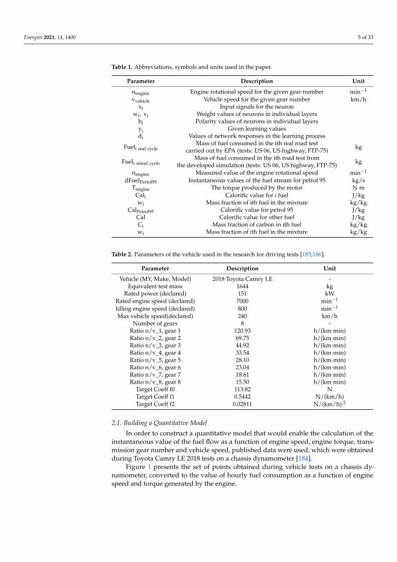
Table 2. Parameters of the vehicle used in the research for driving tests [185,186].
Parameter Description Unit
Vehicle (MY, Make, Model) 2018 Toyota Camry LE -Equivalent test mass 1644 kg
Rated power (declared) 151 kWRated engine speed (declared) 7000 min−1
Idling engine speed (declared) 800 min−1
Max vehicle speed(declared) 240 km/hNumber of gears 8 -
Ratio n/v_1, gear 1 120.93 h/(km·min)Ratio n/v_2, gear 2 69.75 h/(km·min)Ratio n/v_3, gear 3 44.92 h/(km·min)Ratio n/v_4, gear 4 33.54 h/(km·min)Ratio n/v_5, gear 5 28.10 h/(km·min)Ratio n/v_6, gear 6 23.04 h/(km·min)Ratio n/v_7, gear 7 18.61 h/(km·min)Ratio n/v_8, gear 8 15.50 h/(km·min)
Target Coeff f0 113.82 NTarget Coeff f1 0.5442 N/(km/h)Target Coeff f2 0.02811 N/(km/h) 2
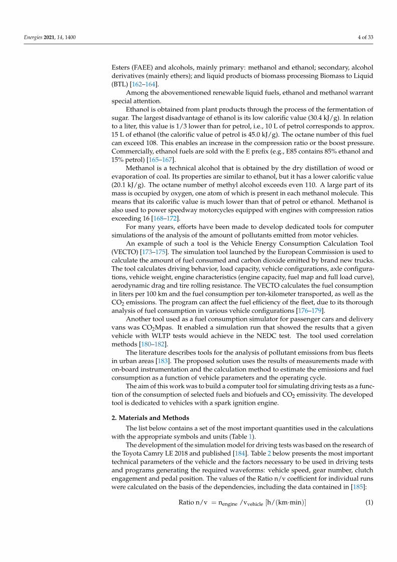
2.1. Building a Quantitative Model
In order to construct a quantitative model that would enable the calculation of theinstantaneous value of the fuel flow as a function of engine speed, engine torque, trans-mission gear number and vehicle speed, published data were used, which were obtainedduring Toyota Camry LE 2018 tests on a chassis dynamometer [184].
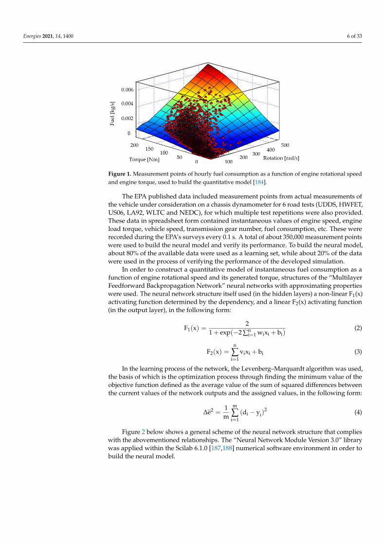
Figure 1 presents the set of points obtained during vehicle tests on a chassis dy-namometer, converted to the value of hourly fuel consumption as a function of enginespeed and torque generated by the engine.
Energies 2021, 14, 1400 6 of 33
Energies 2021, 14, x FOR PEER REVIEW 6 of 33
Figure 1 presents the set of points obtained during vehicle tests on a chassis dyna-mometer, converted to the value of hourly fuel consumption as a function of engine speed and torque generated by the engine.
The EPA published data included measurement points from actual measurements of the vehicle under consideration on a chassis dynamometer for 6 road tests (UDDS, HWFET, US06, LA92, WLTC and NEDC), for which multiple test repetitions were also provided. These data in spreadsheet form contained instantaneous values of engine speed, engine load torque, vehicle speed, transmission gear number, fuel consumption, etc. These were recorded during the EPA’s surveys every 0.1 s. A total of about 350,000 measurement points were used to build the neural model and verify its performance. To build the neural model, about 80% of the available data were used as a learning set, while about 20% of the data were used in the process of verifying the performance of the devel-oped simulation.
Figure 1. Measurement points of hourly fuel consumption as a function of engine rotational speed and engine torque, used to build the quantitative model [184].
In order to construct a quantitative model of instantaneous fuel consumption as a function of engine rotational speed and its generated torque, structures of the “Multilayer Feedforward Backpropagation Network” neural networks with approximating properties were used. The neural network structure itself used (in the hidden layers) a non-linear F1(x) activating function determined by the dependency, and a linear F2(x) activating func-tion (in the output layer), in the following form: F (x) = 21 exp( 2 ∑ w x b ) (2)
F (x) = v x b (3)
In the learning process of the network, the Levenberg–Marquardt algorithm was used, the basis of which is the optimization process through finding the minimum value of the objective function defined as the average value of the sum of squared differences between the current values of the network outputs and the assigned values, in the following form:
∆e = 1m (d y ) (4)
Figure 2 below shows a general scheme of the neural network structure that complies with the abovementioned relationships. The “Neural Network Module Version 3.0” li-brary was applied within the Scilab 6.1.0 [187,188] numerical software environment in order to build the neural model.
Figure 1. Measurement points of hourly fuel consumption as a function of engine rotational speedand engine torque, used to build the quantitative model [184].
The EPA published data included measurement points from actual measurements ofthe vehicle under consideration on a chassis dynamometer for 6 road tests (UDDS, HWFET,US06, LA92, WLTC and NEDC), for which multiple test repetitions were also provided.These data in spreadsheet form contained instantaneous values of engine speed, engineload torque, vehicle speed, transmission gear number, fuel consumption, etc. These wererecorded during the EPA’s surveys every 0.1 s. A total of about 350,000 measurement pointswere used to build the neural model and verify its performance. To build the neural model,about 80% of the available data were used as a learning set, while about 20% of the datawere used in the process of verifying the performance of the developed simulation.
In order to construct a quantitative model of instantaneous fuel consumption as afunction of engine rotational speed and its generated torque, structures of the “MultilayerFeedforward Backpropagation Network” neural networks with approximating propertieswere used. The neural network structure itself used (in the hidden layers) a non-linear F1(x)activating function determined by the dependency, and a linear F2(x) activating function(in the output layer), in the following form:
F1(x) =2
1 + exp(−2 ∑ni=1 wixi + bi)
(2)
F2(x) =n
∑i=1
vixi + bi (3)
In the learning process of the network, the Levenberg–Marquardt algorithm was used,the basis of which is the optimization process through finding the minimum value of theobjective function defined as the average value of the sum of squared differences betweenthe current values of the network outputs and the assigned values, in the following form:
∆e2 =1m
m
∑i=1
(di − yi)2 (4)
Figure 2 below shows a general scheme of the neural network structure that complieswith the abovementioned relationships. The “Neural Network Module Version 3.0” librarywas applied within the Scilab 6.1.0 [187,188] numerical software environment in order tobuild the neural model.
Energies 2021, 14, 1400 7 of 33Energies 2021, 14, x FOR PEER REVIEW 7 of 33
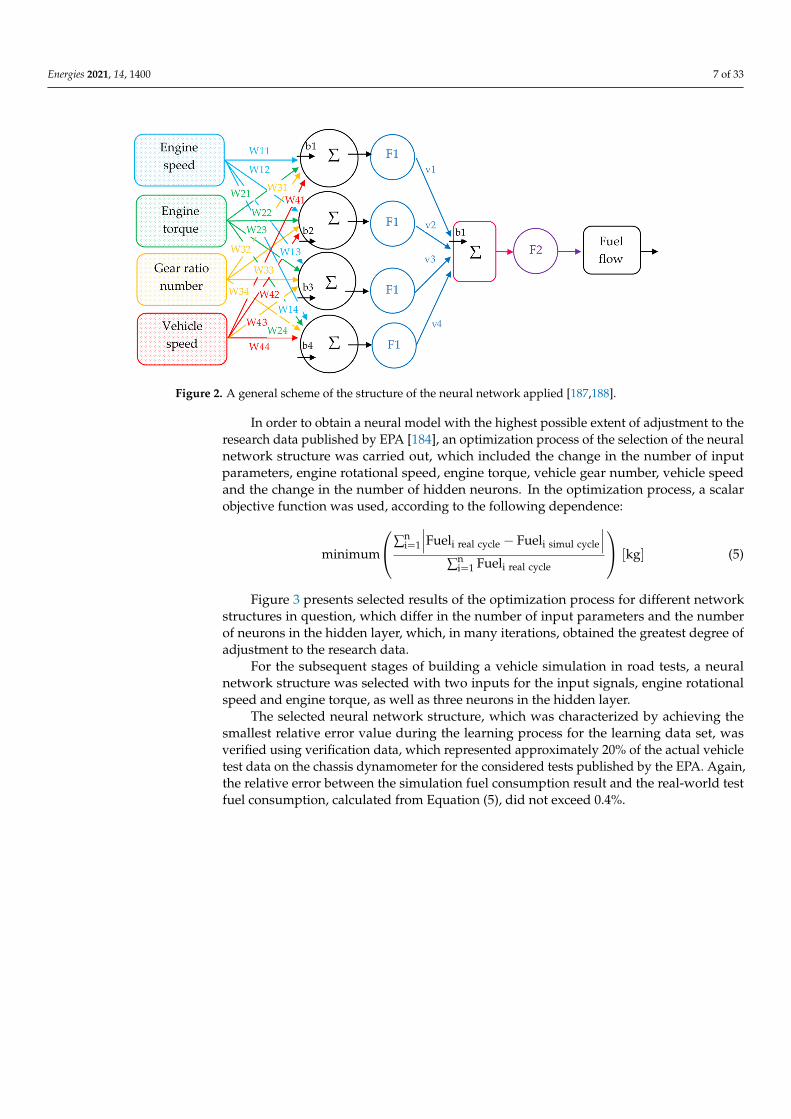
Figure 2. A general scheme of the structure of the neural network applied [187,188].
In order to obtain a neural model with the highest possible extent of adjustment to the research data published by EPA [184], an optimization process of the selection of the neural network structure was carried out, which included the change in the number of input parameters, engine rotational speed, engine torque, vehicle gear number, vehicle speed and the change in the number of hidden neurons. In the optimization process, a scalar objective function was used, according to the following dependence: minimum ∑ Fuel Fuel ∑ Fuel kg (5)
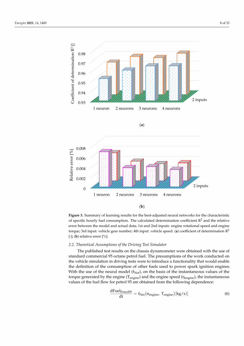
Figure 3 presents selected results of the optimization process for different network structures in question, which differ in the number of input parameters and the number of neurons in the hidden layer, which, in many iterations, obtained the greatest degree of adjustment to the research data.
For the subsequent stages of building a vehicle simulation in road tests, a neural net-work structure was selected with two inputs for the input signals, engine rotational speed and engine torque, as well as three neurons in the hidden layer.
The selected neural network structure, which was characterized by achieving the smallest relative error value during the learning process for the learning data set, was verified using verification data, which represented approximately 20% of the actual vehi-cle test data on the chassis dynamometer for the considered tests published by the EPA. Again, the relative error between the simulation fuel consumption result and the real-world test fuel consumption, calculated from Equation (5), did not exceed 0.4%.
Figure 2. A general scheme of the structure of the neural network applied [187,188].
In order to obtain a neural model with the highest possible extent of adjustment to theresearch data published by EPA [184], an optimization process of the selection of the neuralnetwork structure was carried out, which included the change in the number of inputparameters, engine rotational speed, engine torque, vehicle gear number, vehicle speedand the change in the number of hidden neurons. In the optimization process, a scalarobjective function was used, according to the following dependence:
minimum
∑ni=1
∣∣∣Fueli real cycle − Fueli simul cycle
∣∣∣∑n
i=1 Fueli real cycle
[kg] (5)
Figure 3 presents selected results of the optimization process for different networkstructures in question, which differ in the number of input parameters and the numberof neurons in the hidden layer, which, in many iterations, obtained the greatest degree ofadjustment to the research data.
For the subsequent stages of building a vehicle simulation in road tests, a neuralnetwork structure was selected with two inputs for the input signals, engine rotationalspeed and engine torque, as well as three neurons in the hidden layer.
The selected neural network structure, which was characterized by achieving thesmallest relative error value during the learning process for the learning data set, wasverified using verification data, which represented approximately 20% of the actual vehicletest data on the chassis dynamometer for the considered tests published by the EPA. Again,the relative error between the simulation fuel consumption result and the real-world testfuel consumption, calculated from Equation (5), did not exceed 0.4%.
Energies 2021, 14, 1400 8 of 33
Energies 2021, 14, x FOR PEER REVIEW 8 of 33
(a)
(b)
Figure 3. Summary of learning results for the best-adjusted neural networks for the characteristic of specific hourly fuel consumption. The calculated determination coefficient R2 and the relative error between the model and actual data; 1st and 2nd inputs: engine rotational speed and engine torque; 3rd input: vehicle gear number; 4th input: vehicle speed: (a) coefficient of determination R2
[-]; (b) relative error [%].
2.2. Theoretical Assumptions of the Driving Test Simulator The published test results on the chassis dynamometer were obtained with the use
of standard commercial 95 octane petrol fuel. The presumptions of the work conducted on the vehicle simulation in driving tests were to introduce a functionality that would enable the definition of the consumption of other fuels used to power spark ignition en-gines. With the use of the neural model (fNet), on the basis of the instantaneous values of the torque generated by the engine (Tengine) and the engine speed (ηengine), the instantaneous values of the fuel flow for petrol 95 are obtained from the following dependence: dFueldt = f n , T kg/s) (6)
Then, the simulation calculates the calorific value, in the case of using a fuel other than petrol 95 or fuel mixtures from the relationship:
2 inputs0.93
0.94
0.95
0.96
0.97
0.98
1 neuron 2 neurons 3 neurons 4 neurons
Coe
ffici
ent o
f det
erm
inat
ion
R2
[]
2 inputs0
0.002
0.004
0.006
0.008
1 neuron 2 neurons 3 neurons 4 neurons
Rela
tive
erro
r [%
]
Figure 3. Summary of learning results for the best-adjusted neural networks for the characteristicof specific hourly fuel consumption. The calculated determination coefficient R2 and the relativeerror between the model and actual data; 1st and 2nd inputs: engine rotational speed and enginetorque; 3rd input: vehicle gear number; 4th input: vehicle speed: (a) coefficient of determination R2
[-]; (b) relative error [%].
2.2. Theoretical Assumptions of the Driving Test Simulator
The published test results on the chassis dynamometer were obtained with the use ofstandard commercial 95 octane petrol fuel. The presumptions of the work conducted onthe vehicle simulation in driving tests were to introduce a functionality that would enablethe definition of the consumption of other fuels used to power spark ignition engines.With the use of the neural model (fNet), on the basis of the instantaneous values of thetorque generated by the engine (Tengine) and the engine speed (ηengine), the instantaneousvalues of the fuel flow for petrol 95 are obtained from the following dependence:
dFuelPetrol95dt
= fNet(nengine, Tengine
)[kg/s)] (6)
Energies 2021, 14, 1400 9 of 33
Then, the simulation calculates the calorific value, in the case of using a fuel otherthan petrol 95 or fuel mixtures from the relationship:
Cal =n
∑i=1
wi·Cali [J/kg] (7)
It was assumed in the calculations that, for the instantaneous load value arising fromthe rotational engine speed and the engine-generated torque, a stream of another fuel mustprovide the same amount of energy over time as in the case of petrol 95. The efficiency ofoperation in the case of an engine powered by other fuels remains the same as for petrol 95,for each given calculation point. In this case, the instantaneous stream of fuels other thanpetrol 95 is calculated from the following dependence:
dFueldt
=dFuelPetrol95
dtCalPetrol95
Cal[kg/s)] (8)
Table 3 presents the basic parameters of the fuels used in the simulation:
Table 3. Basic parameters of the fuels used in the simulation [189–193].
Parameter Petrol 95 Ethanol Methanol DME CNG LPG
Calorific [MJ/kg] 43.5 26.7 19.93 28.4 50.0 46.3Carbon [%] 86.4 52.1 37.5 52.1 74.9 81.7
Hydrogen [%] 13.6 13.1 12.6 13.1 25.1 18.3Oxygen [%] 0.0 34.7 49.9 34.7 0.0 0.0
The presented properties of CNG fuel refer to the mixture which is used to powervehicles in a compressed form to the value of about 20MPa, containing 96–98% of methanewith a minimum amount of other polluting gases and water vapor.
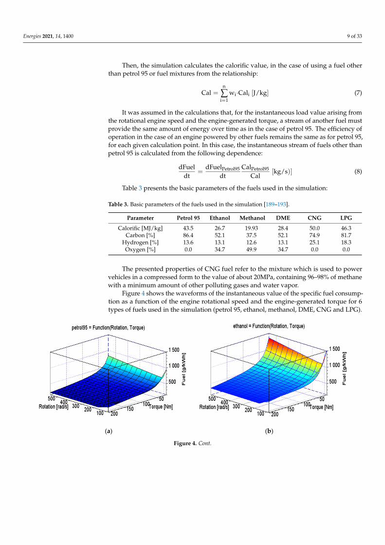
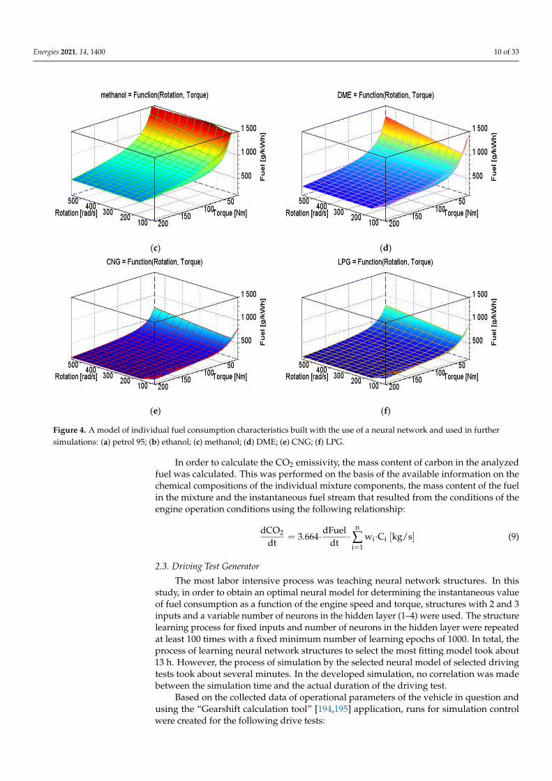
Figure 4 shows the waveforms of the instantaneous value of the specific fuel consump-tion as a function of the engine rotational speed and the engine-generated torque for 6types of fuels used in the simulation (petrol 95, ethanol, methanol, DME, CNG and LPG).
Energies 2021, 14, x FOR PEER REVIEW 9 of 33
Cal = w · Cal J/kg (7)
It was assumed in the calculations that, for the instantaneous load value arising from the rotational engine speed and the engine-generated torque, a stream of another fuel must provide the same amount of energy over time as in the case of petrol 95. The effi-ciency of operation in the case of an engine powered by other fuels remains the same as for petrol 95, for each given calculation point. In this case, the instantaneous stream of fuels other than petrol 95 is calculated from the following dependence: dFueldt = dFueldt Cal Cal kg/s) (8)
Table 3 presents the basic parameters of the fuels used in the simulation:
Table 3. Basic parameters of the fuels used in the simulation [189–193].
Parameter Petrol 95 Ethanol Methanol DME CNG LPG Calorific [MJ/kg] 43.5 26.7 19.93 28.4 50.0 46.3
Carbon [%] 86.4 52.1 37.5 52.1 74.9 81.7 Hydrogen [%] 13.6 13.1 12.6 13.1 25.1 18.3
Oxygen [%] 0.0 34.7 49.9 34.7 0.0 0.0
The presented properties of CNG fuel refer to the mixture which is used to power vehicles in a compressed form to the value of about 20MPa, containing 96–98% of methane with a minimum amount of other polluting gases and water vapor.
Figure 4 shows the waveforms of the instantaneous value of the specific fuel con-sumption as a function of the engine rotational speed and the engine-generated torque for 6 types of fuels used in the simulation (petrol 95, ethanol, methanol, DME, CNG and LPG).
(a) (b)
Figure 4. Cont.
Energies 2021, 14, 1400 10 of 33Energies 2021, 14, x FOR PEER REVIEW 10 of 33
(c) (d)
(e) (f)
Figure 4. A model of individual fuel consumption characteristics built with the use of a neural network and used in further simulations: (a) petrol 95; (b) ethanol; (c) methanol; (d) DME; (e) CNG; (f) LPG.
In order to calculate the CO2 emissivity, the mass content of carbon in the analyzed fuel was calculated. This was performed on the basis of the available information on the chemical compositions of the individual mixture components, the mass content of the fuel in the mixture and the instantaneous fuel stream that resulted from the conditions of the engine operation conditions using the following relationship: dCOdt = 3.664 · dFueldt · w · C kg/s (9)
2.3. Driving Test Generator The most labor intensive process was teaching neural network structures. In this
study, in order to obtain an optimal neural model for determining the instantaneous value of fuel consumption as a function of the engine speed and torque, structures with 2 and 3 inputs and a variable number of neurons in the hidden layer (1–4) were used. The struc-ture learning process for fixed inputs and number of neurons in the hidden layer were repeated at least 100 times with a fixed minimum number of learning epochs of 1000. In total, the process of learning neural network structures to select the most fitting model took about 13 h. However, the process of simulation by the selected neural model of se-lected driving tests took about several minutes. In the developed simulation, no correla-tion was made between the simulation time and the actual duration of the driving test.
Figure 4. A model of individual fuel consumption characteristics built with the use of a neural network and used in furthersimulations: (a) petrol 95; (b) ethanol; (c) methanol; (d) DME; (e) CNG; (f) LPG.
In order to calculate the CO2 emissivity, the mass content of carbon in the analyzedfuel was calculated. This was performed on the basis of the available information on thechemical compositions of the individual mixture components, the mass content of the fuelin the mixture and the instantaneous fuel stream that resulted from the conditions of theengine operation conditions using the following relationship:
dCO2
dt= 3.664·dFuel
dt·
n
∑i=1
wi·Ci [kg/s] (9)
2.3. Driving Test Generator
The most labor intensive process was teaching neural network structures. In thisstudy, in order to obtain an optimal neural model for determining the instantaneous valueof fuel consumption as a function of the engine speed and torque, structures with 2 and 3inputs and a variable number of neurons in the hidden layer (1–4) were used. The structurelearning process for fixed inputs and number of neurons in the hidden layer were repeatedat least 100 times with a fixed minimum number of learning epochs of 1000. In total, theprocess of learning neural network structures to select the most fitting model took about13 h. However, the process of simulation by the selected neural model of selected drivingtests took about several minutes. In the developed simulation, no correlation was madebetween the simulation time and the actual duration of the driving test.
Based on the collected data of operational parameters of the vehicle in question andusing the “Gearshift calculation tool” [194,195] application, runs for simulation controlwere created for the following drive tests:
Energies 2021, 14, 1400 11 of 33
• US 06—The US06 (SFTP) [196,197];• US highway—Highway Fuel Economy Driving Schedule (HWFET) [198–200];• FTP-75—EPA Federal Test Procedure [201–203];• NEDC—New European Driving Cycle (NEDC) [204–206];• US SC03—The SC03 (SFTP) [207,208];• Random Cycle Low (×05)—a test generated from a procedure in the WLTP Random
Cycle Generator tool [209,210];• Random Cycle High (×95)—a test generated from a procedure in the WLTP Random
Cycle Generator tool [211,212];• MAC TP cycle—mobile air conditioning (MAC) [213,214];• CADC—Artemis cycle definitions, includes the following cycles: urban, rural road
and motorway [215–217];• CADC w/o mot—Artemis cycle definitions, includes the following cycles: Urban,
Rural Road. Does not include: Motorway [215–217];• CADC abridged—same as Artemis cycle definitions, includes the following cycles:
urban, rural road and motorway. The duration time was shortened, similar to CADCw/o mot [215–217];
• WLTC 3b random—WLTP for class 3 vehicles with the engine power above34 W/kg [218–221].
Upon entering the complete information about the vehicle, the program is ready togenerate the necessary waveforms in the time domain, which in turn enable the deter-mination of the instantaneous operating parameters of the program in question. Thesewaveforms were then exported to text files. The instantaneous waveforms of the followingquantities were used in the further stages of the simulation: simulation time [s]; enginespeed [rpm]; power produced by the engine [kW]; torque generated by the engine [Nm]—avalue calculated on the basis of the engine rotational speed and engine power; gear number[-]; vehicle speed [km/h].
2.4. Simulator
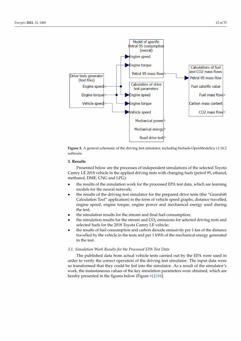
A driving test simulator was developed in OpenModelica v1.16.2, based on theanalysis of the data created with the use of the “Gearshift calculation tool” programme, theresults of the process of neural network structure optimization and the properties of thetested biofuels [222]. The simulator is made up of blocks that are responsible for individualfunctionalities, and its connection diagram is presented in Figure 5 below:
• Drive tests generator (text files)—responsible for loading files with data that controlthe selected driving test process from a text file created with the use of the “Gearshiftcalculation tool” application. It is also responsible for converting the read data toother formats compatible with OpenModelica v1.16.2. The following parameters arethen relayed to the following calculation modules of the simulation: engine speed,engine torque, vehicle speed;
• Model of specific consumption (neural)—this block calculates the instantaneous valuesof petrol 95 mass flow and relays this parameter to the next block, based on thequantities which characterize the engine operating parameters: engine speed, enginetorque and the prepared neural network structure;
• Calculations of fuel and CO2 mass flows—this block is responsible for calculatingthe streams of the tested biofuels which are necessary to power the engine in thedriving test. This is achieved using the petrol 95 mass flow parameter and the fuelcalorific value characteristic for the fuel in question calculated in the previous block.This block also calculates the CO2 emission stream with the use of the carbon masscontent property and the instantaneous fuel stream;
• Calculation of driving test parameters—on the basis of the driving test parameters,this block calculates the distance covered by the vehicle during the test, the powergenerated by the engine and the mechanical energy generated during the test.
Energies 2021, 14, 1400 12 of 33
Energies 2021, 14, x FOR PEER REVIEW 12 of 33
• Calculation of driving test parameters—on the basis of the driving test parameters,this block calculates the distance covered by the vehicle during the test, the powergenerated by the engine and the mechanical energy generated during the test.
Figure 5. A general schematic of the driving test simulator, including biofuels OpenModelica v1.16.2 software.
3. ResultsPresented below are the processes of independent simulations of the selected Toyota
Camry LE 2018 vehicle in the applied driving tests with changing fuels (petrol 95, ethanol, methanol, DME, CNG and LPG): • the results of the simulation work for the processed EPA test data, which are learning
models for the neural network;• the results of the driving test simulator for the prepared drive tests (the “Gearshift Cal-
culation Tool” application) in the form of vehicle speed graphs, distance travelled, en-gine speed, engine torque, engine power and mechanical energy used during the test;
• the simulation results for the stream and final fuel consumption;• the simulation results for the stream and CO2 emissions for selected driving tests and
selected fuels for the 2018 Toyota Camry LE vehicle;• the results of fuel consumption and carbon dioxide emissivity per 1 km of the dis-
tance travelled by the vehicle in the tests and per 1 kWh of the mechanical energygenerated in the test.
3.1. Simulation Work Results for the Processed EPA Test Data The published data from actual vehicle tests carried out by the EPA were used in
order to verify the correct operation of the driving test simulator. The input data were so transformed that they could be fed into the simulator. As a result of the simulator’s work, the instantaneous values of the key simulation parameters were obtained, which are hereby presented in the figures below (Figure 6) [184].
Figure 5. A general schematic of the driving test simulator, including biofuels OpenModelica v1.16.2software.
3. Results
Presented below are the processes of independent simulations of the selected ToyotaCamry LE 2018 vehicle in the applied driving tests with changing fuels (petrol 95, ethanol,methanol, DME, CNG and LPG):
• the results of the simulation work for the processed EPA test data, which are learningmodels for the neural network;
• the results of the driving test simulator for the prepared drive tests (the “GearshiftCalculation Tool” application) in the form of vehicle speed graphs, distance travelled,engine speed, engine torque, engine power and mechanical energy used duringthe test;
• the simulation results for the stream and final fuel consumption;• the simulation results for the stream and CO2 emissions for selected driving tests and
selected fuels for the 2018 Toyota Camry LE vehicle;• the results of fuel consumption and carbon dioxide emissivity per 1 km of the distance
travelled by the vehicle in the tests and per 1 kWh of the mechanical energy generatedin the test.
3.1. Simulation Work Results for the Processed EPA Test Data
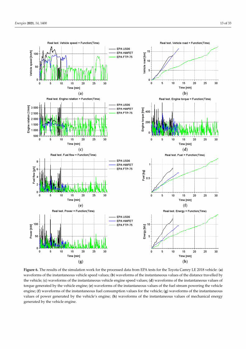
The published data from actual vehicle tests carried out by the EPA were used inorder to verify the correct operation of the driving test simulator. The input data wereso transformed that they could be fed into the simulator. As a result of the simulator’swork, the instantaneous values of the key simulation parameters were obtained, which arehereby presented in the figures below (Figure 6) [184].
Energies 2021, 14, 1400 13 of 33Energies 2021, 14, x FOR PEER REVIEW 13 of 33
(a) (b)
(c) (d)
(e) (f)
(g) (h)
Figure 6. The results of the simulation work for the processed data from EPA tests for the Toyota Camry LE 2018 vehicle: (a) waveforms of the instantaneous vehicle speed values; (b) waveforms of the instantaneous values of the distance trav-elled by the vehicle; (c) waveforms of the instantaneous vehicle engine speed values; (d) waveforms of the instantaneous values of torque generated by the vehicle engine; (e) waveforms of the instantaneous values of the fuel stream powering the vehicle engine; (f) waveforms of the instantaneous fuel consumption values for the vehicle; (g) waveforms of the in-stantaneous values of power generated by the vehicle’s engine; (h) waveforms of the instantaneous values of mechanical energy generated by the vehicle engine.
3.2. Simulation Work Results for the Driving Tests Performed On the basis of the prepared input data, using the “Gearshift Calculation Tool” soft-
ware, simulations of selected driving tests were carried out for the vehicle in question. Figure 7 below shows the waveforms of the instantaneous vehicle speed values in the test.
Figure 6. The results of the simulation work for the processed data from EPA tests for the Toyota Camry LE 2018 vehicle: (a)waveforms of the instantaneous vehicle speed values; (b) waveforms of the instantaneous values of the distance travelled bythe vehicle; (c) waveforms of the instantaneous vehicle engine speed values; (d) waveforms of the instantaneous values oftorque generated by the vehicle engine; (e) waveforms of the instantaneous values of the fuel stream powering the vehicleengine; (f) waveforms of the instantaneous fuel consumption values for the vehicle; (g) waveforms of the instantaneousvalues of power generated by the vehicle’s engine; (h) waveforms of the instantaneous values of mechanical energygenerated by the vehicle engine.
Energies 2021, 14, 1400 14 of 33
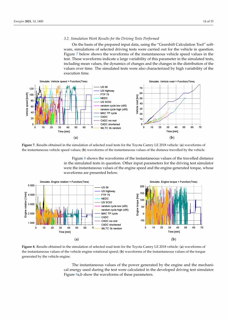
3.2. Simulation Work Results for the Driving Tests Performed
On the basis of the prepared input data, using the “Gearshift Calculation Tool” soft-ware, simulations of selected driving tests were carried out for the vehicle in question.Figure 7 below shows the waveforms of the instantaneous vehicle speed values in thetest. These waveforms indicate a large variability of this parameter in the simulated tests,including mean values, the dynamics of changes and the changes in the distribution of thevalues over time. The simulated tests were also characterized by high variability of theexecution time.
Energies 2021, 14, x FOR PEER REVIEW 14 of 33
These waveforms indicate a large variability of this parameter in the simulated tests, in-cluding mean values, the dynamics of changes and the changes in the distribution of the values over time. The simulated tests were also characterized by high variability of the execution time.
(a) (b)
Figure 7. Results obtained in the simulation of selected road tests for the Toyota Camry LE 2018 vehicle: (a) waveforms of the instantaneous vehicle speed values; (b) waveforms of the instantaneous values of the distance travelled by the vehicle.
Figure 8 shows the waveforms of the instantaneous values of the travelled distance in the simulated tests in question. Other input parameters for the driving test simulator were the instantaneous values of the engine speed and the engine-generated torque, whose waveforms are presented below.
(a) (b)
Figure 8. Results obtained in the simulation of selected road tests for the Toyota Camry LE 2018 vehicle: (a) waveforms of the instantaneous values of the vehicle engine rotational speed; (b) waveforms of the instantaneous values of the torque generated by the vehicle engine.
The instantaneous values of the power generated by the engine and the mechanical energy used during the test were calculated in the developed driving test simulator. Fig-ure 9a,b show the waveforms of these parameters.
Figure 7. Results obtained in the simulation of selected road tests for the Toyota Camry LE 2018 vehicle: (a) waveforms ofthe instantaneous vehicle speed values; (b) waveforms of the instantaneous values of the distance travelled by the vehicle.
Figure 8 shows the waveforms of the instantaneous values of the travelled distancein the simulated tests in question. Other input parameters for the driving test simulatorwere the instantaneous values of the engine speed and the engine-generated torque, whosewaveforms are presented below.
Energies 2021, 14, x FOR PEER REVIEW 14 of 33
These waveforms indicate a large variability of this parameter in the simulated tests, in-cluding mean values, the dynamics of changes and the changes in the distribution of the values over time. The simulated tests were also characterized by high variability of the execution time.
(a) (b)
Figure 7. Results obtained in the simulation of selected road tests for the Toyota Camry LE 2018 vehicle: (a) waveforms of the instantaneous vehicle speed values; (b) waveforms of the instantaneous values of the distance travelled by the vehicle.
Figure 8 shows the waveforms of the instantaneous values of the travelled distance in the simulated tests in question. Other input parameters for the driving test simulator were the instantaneous values of the engine speed and the engine-generated torque, whose waveforms are presented below.
(a) (b)
Figure 8. Results obtained in the simulation of selected road tests for the Toyota Camry LE 2018 vehicle: (a) waveforms of the instantaneous values of the vehicle engine rotational speed; (b) waveforms of the instantaneous values of the torque generated by the vehicle engine.
The instantaneous values of the power generated by the engine and the mechanical energy used during the test were calculated in the developed driving test simulator. Fig-ure 9a,b show the waveforms of these parameters.
Figure 8. Results obtained in the simulation of selected road tests for the Toyota Camry LE 2018 vehicle: (a) waveforms ofthe instantaneous values of the vehicle engine rotational speed; (b) waveforms of the instantaneous values of the torquegenerated by the vehicle engine.
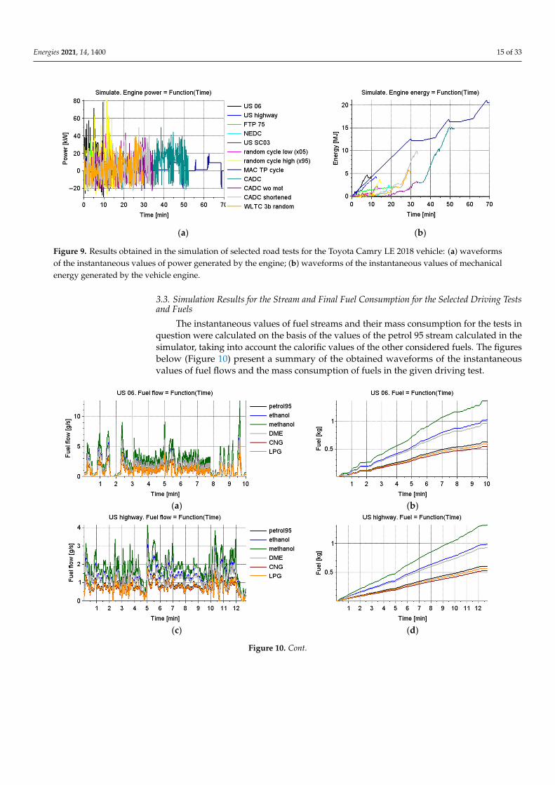
The instantaneous values of the power generated by the engine and the mechani-cal energy used during the test were calculated in the developed driving test simulator.Figure 9a,b show the waveforms of these parameters.
Energies 2021, 14, 1400 15 of 33Energies 2021, 14, x FOR PEER REVIEW 15 of 33
(a) (b)
Figure 9. Results obtained in the simulation of selected road tests for the Toyota Camry LE 2018 vehicle: (a) waveforms of the instantaneous values of power generated by the engine; (b) waveforms of the instantaneous values of mechanical energy generated by the vehicle engine.
3.3. Simulation Results for the Stream and Final Fuel Consumption for the Selected Driving Tests and Fuels
The instantaneous values of fuel streams and their mass consumption for the tests in question were calculated on the basis of the values of the petrol 95 stream calculated in the simulator, taking into account the calorific values of the other considered fuels. The figures below (Figure 10) present a summary of the obtained waveforms of the instanta-neous values of fuel flows and the mass consumption of fuels in the given driving test.
(a) (b)
(c) (d)
Figure 9. Results obtained in the simulation of selected road tests for the Toyota Camry LE 2018 vehicle: (a) waveformsof the instantaneous values of power generated by the engine; (b) waveforms of the instantaneous values of mechanicalenergy generated by the vehicle engine.
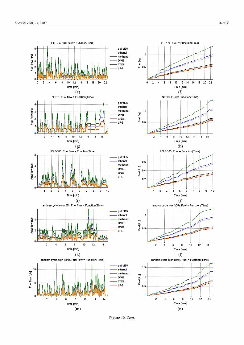
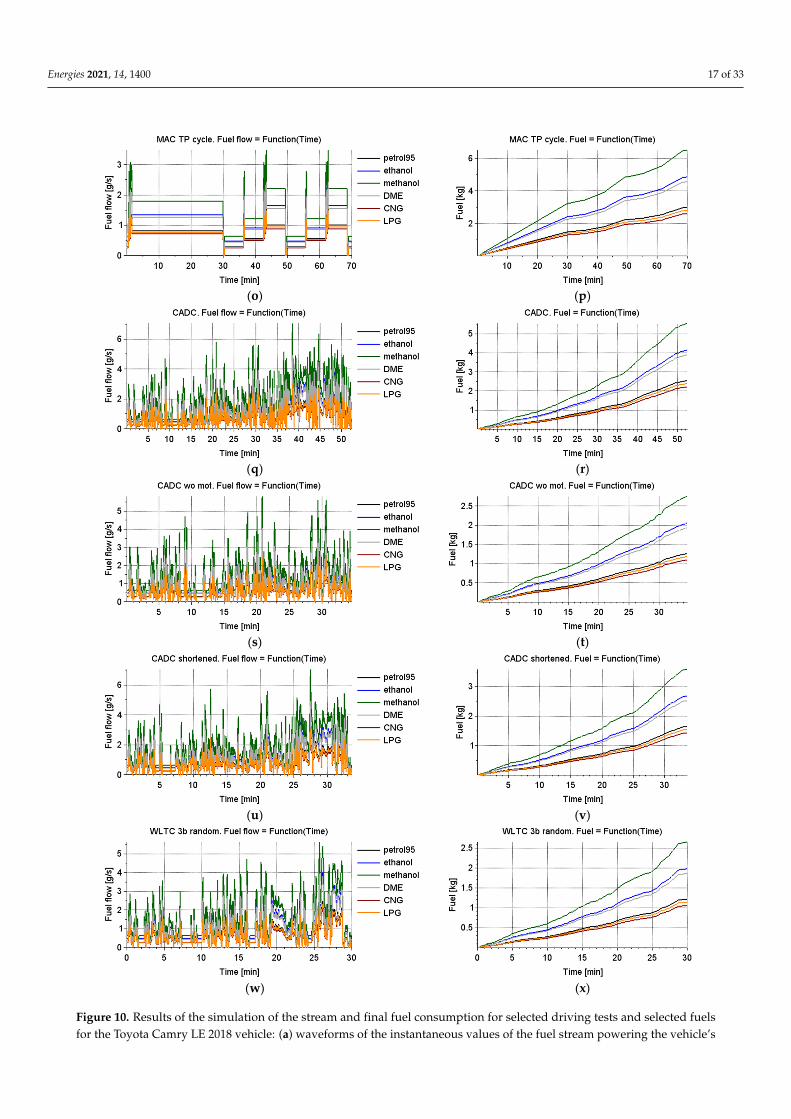
3.3. Simulation Results for the Stream and Final Fuel Consumption for the Selected Driving Testsand Fuels
The instantaneous values of fuel streams and their mass consumption for the tests inquestion were calculated on the basis of the values of the petrol 95 stream calculated in thesimulator, taking into account the calorific values of the other considered fuels. The figuresbelow (Figure 10) present a summary of the obtained waveforms of the instantaneousvalues of fuel flows and the mass consumption of fuels in the given driving test.
Energies 2021, 14, x FOR PEER REVIEW 15 of 33
(a) (b)
Figure 9. Results obtained in the simulation of selected road tests for the Toyota Camry LE 2018 vehicle: (a) waveforms of the instantaneous values of power generated by the engine; (b) waveforms of the instantaneous values of mechanical energy generated by the vehicle engine.
3.3. Simulation Results for the Stream and Final Fuel Consumption for the Selected Driving Tests and Fuels
The instantaneous values of fuel streams and their mass consumption for the tests in question were calculated on the basis of the values of the petrol 95 stream calculated in the simulator, taking into account the calorific values of the other considered fuels. The figures below (Figure 10) present a summary of the obtained waveforms of the instanta-neous values of fuel flows and the mass consumption of fuels in the given driving test.
(a) (b)
(c) (d)
Figure 10. Cont.
Energies 2021, 14, 1400 16 of 33Energies 2021, 14, x FOR PEER REVIEW 16 of 33
(e) (f)
(g) (h)
(i) (j)
(k) (l)
(m) (n)
Figure 10. Cont.
Energies 2021, 14, 1400 17 of 33Energies 2021, 14, x FOR PEER REVIEW 17 of 33
(o) (p)
(q) (r)
(s) (t)
(u) (v)
(w) (x)
Figure 10. Results of the simulation of the stream and final fuel consumption for selected driving tests and selected fuelsfor the Toyota Camry LE 2018 vehicle: (a) waveforms of the instantaneous values of the fuel stream powering the vehicle’s
Energies 2021, 14, 1400 18 of 33
engine, obtained in the simulation of the US 06 road test; (b) waveforms of the instantaneous values of fuel consumptionfor the vehicle, obtained in the simulation of the US 06 road test; (c) waveforms of the instantaneous values of the fuelstream powering the vehicle’s engine, obtained in the simulation of the US highway road test; (d) waveforms of theinstantaneous values fuel consumption values for the vehicle, obtained in the US highway test simulation; (e) waveforms ofthe instantaneous values of the fuel stream powering the vehicle’s engine, obtained in the simulation of the FTP-75 road test;(f) waveforms of the instantaneous values of fuel consumption for the vehicle, obtained in the simulation of the FTP-75 roadtest; (g) waveforms of the instantaneous values of the fuel stream powering the vehicle’s engine, obtained in the simulationof the New European Driving Cycle (NEDC) road test; (h) waveforms of the instantaneous values of fuel consumption forthe vehicle, obtained in the simulation of the NEDC road test; (i) waveforms of the instantaneous values of the fuel streampowering the vehicle’s engine, obtained in the simulation of the US SC03 road test; (j) waveforms of the instantaneousvalues of fuel consumption for the vehicle, obtained in the simulation of the US SC03 road test; (k) waveforms of theinstantaneous values of the fuel stream powering the vehicle’s engine, obtained in the simulation of the Random Cycle Low(×05) road test; (l) waveforms of the instantaneous values of fuel consumption for the vehicle, obtained in the simulation ofthe Random Cycle Low (×05) road test; (m) waveforms of the instantaneous values of the fuel stream powering the vehicle’sengine, obtained in the simulation of the Random Cycle High (×95) road test; (n) waveforms of the instantaneous values ofthe fuel consumption for the vehicle, obtained in the simulation of the Random Cycle High (×95) road test; (o) waveformsof the instantaneous values of the fuel stream powering the vehicle’s engine, obtained in the simulation of the Mobile AirConditioning Test Procedure (MAC TP) cycle road test; (p) waveforms of the instantaneous values of fuel consumption forthe vehicle, obtained in the simulation of the MAC TP cycle road test; (q) waveforms of the instantaneous values of the fuelstream powering the vehicle’s engine, obtained in the simulation of the Common Artemis Driving Cycles (CADC) road test;(r) waveforms of the instantaneous values of fuel consumption for the vehicle, obtained in the simulation of the CADC roadtest; (s) waveforms of the instantaneous values of the fuel stream powering the vehicle’s engine, obtained in the simulationof the CADC w/o mot road test; (t) waveforms of the instantaneous values of fuel consumption for the vehicle, obtained inthe simulation of the CADC w/o mot road test; (u) waveforms of the instantaneous values of the fuel stream poweringthe vehicle’s engine, obtained in the simulation of the CADC shortened road test; (v) waveforms of the instantaneousvalues of fuel consumption for the vehicle, obtained in the simulation of the CADC shortened road test; (w) waveforms ofthe instantaneous values of the fuel stream powering the vehicle’s engine, obtained in the simulation of the WorldwideHarmonized Light-Duty Vehicles Test Cycles (WLTC) 3b random road test; (x) waveforms of the instantaneous values offuel consumption for the vehicle, obtained in the simulation of the WLTC 3b random road test.
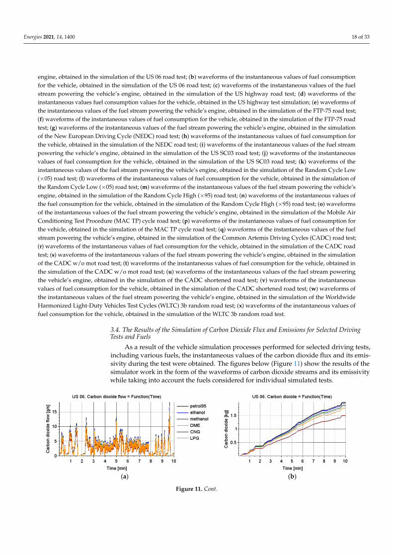
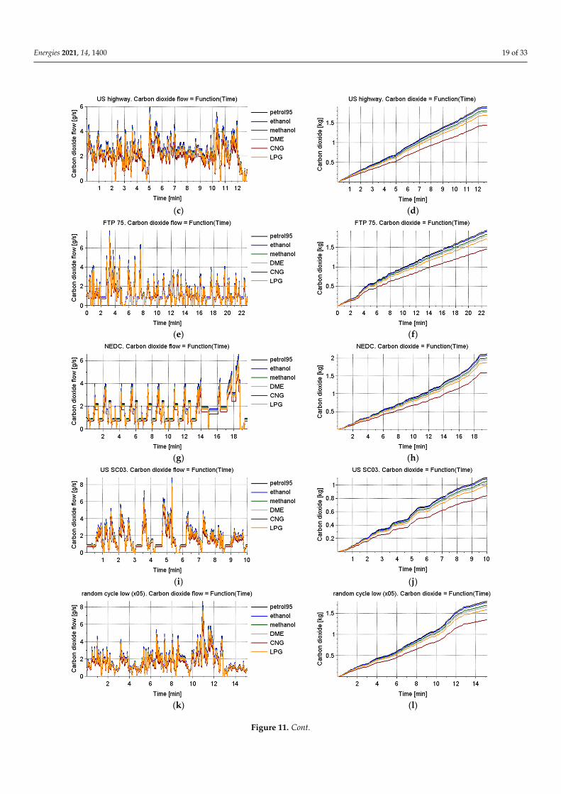
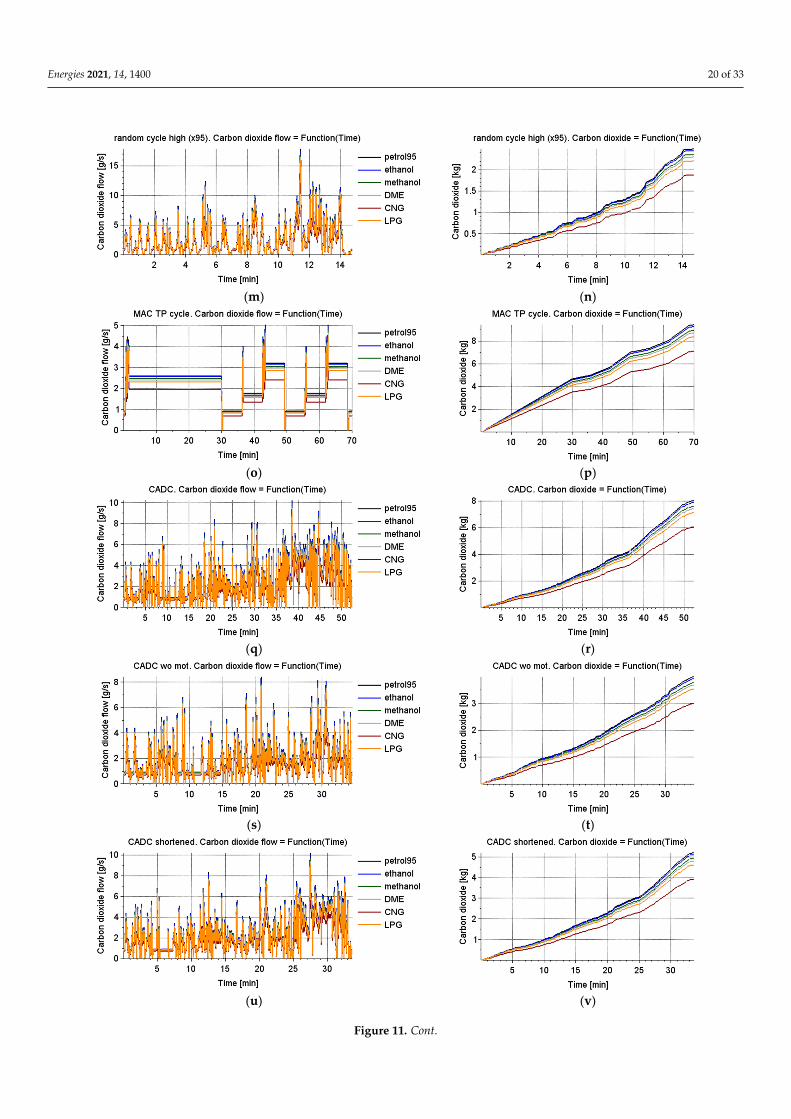
3.4. The Results of the Simulation of Carbon Dioxide Flux and Emissions for Selected DrivingTests and Fuels
As a result of the vehicle simulation processes performed for selected driving tests,including various fuels, the instantaneous values of the carbon dioxide flux and its emis-sivity during the test were obtained. The figures below (Figure 11) show the results of thesimulator work in the form of the waveforms of carbon dioxide streams and its emissivitywhile taking into account the fuels considered for individual simulated tests.
Energies 2021, 14, x FOR PEER REVIEW 18 of 33
Figure 10. Results of the simulation of the stream and final fuel consumption for selected driving tests and selected fuels for the Toyota Camry LE 2018 vehicle: (a) waveforms of the instantaneous values of the fuel stream powering the vehicle’s en-gine, obtained in the simulation of the US 06 road test; (b) waveforms of the instantaneous values of fuel consumption for the vehicle, obtained in the simulation of the US 06 road test; (c) waveforms of the instantaneous values of the fuel stream pow-ering the vehicle’s engine, obtained in the simulation of the US highway road test; (d) waveforms of the instantaneous values fuel consumption values for the vehicle, obtained in the US highway test simulation; (e) waveforms of the instantaneous values of the fuel stream powering the vehicle’s engine, obtained in the simulation of the FTP-75 road test; (f) waveforms of the instantaneous values of fuel consumption for the vehicle, obtained in the simulation of the FTP-75 road test; (g) waveforms of the instantaneous values of the fuel stream powering the vehicle’s engine, obtained in the simulation of the New European Driving Cycle (NEDC) road test; (h) waveforms of the instantaneous values of fuel consumption for the vehicle, obtained in the simulation of the NEDC road test; (i) waveforms of the instantaneous values of the fuel stream powering the vehicle’s engine, obtained in the simulation of the US SC03 road test; (j) waveforms of the instantaneous values of fuel consumption for the vehicle, obtained in the simulation of the US SC03 road test; (k) waveforms of the instantaneous values of the fuel stream powering the vehicle’s engine, obtained in the simulation of the Random Cycle Low (×05) road test; (l) waveforms of the instantaneous values of fuel consumption for the vehicle, obtained in the simulation of the Random Cycle Low (×05) road test; (m) waveforms of the instantaneous values of the fuel stream powering the vehicle’s engine, obtained in the simulation of the Random Cycle High (×95) road test; (n) waveforms of the instantaneous values of the fuel consumption for the vehicle, obtained in the simulation of the Random Cycle High (×95) road test; (o) waveforms of the instantaneous values of the fuel stream powering the vehicle’s engine, obtained in the simulation of the Mobile Air Conditioning Test Procedure (MAC TP) cycle road test; (p) waveforms of the instantaneous values of fuel consumption for the vehicle, obtained in the simulation of the MAC TP cycle road test; (q) waveforms of the instantaneous values of the fuel stream powering the vehicle’s engine, obtained in the simulation of the Common Artemis Driving Cycles (CADC) road test; (r) waveforms of the instantaneous values of fuel consumption for the vehicle, obtained in the simulation of the CADC road test; (s) waveforms of the instanta-neous values of the fuel stream powering the vehicle’s engine, obtained in the simulation of the CADC w/o mot road test; (t) waveforms of the instantaneous values of fuel consumption for the vehicle, obtained in the simulation of the CADC w/o mot road test; (u) waveforms of the instantaneous values of the fuel stream powering the vehicle’s engine, obtained in the simu-lation of the CADC shortened road test; (v) waveforms of the instantaneous values of fuel consumption for the vehicle, ob-tained in the simulation of the CADC shortened road test; (w) waveforms of the instantaneous values of the fuel stream powering the vehicle’s engine, obtained in the simulation of the Worldwide Harmonized Light-Duty Vehicles Test Cycles (WLTC) 3b random road test; (x) waveforms of the instantaneous values of fuel consumption for the vehicle, obtained in the simulation of the WLTC 3b random road test.
3.4. The Results of the Simulation of Carbon Dioxide Flux and Emissions for Selected Driving Tests and Fuels
As a result of the vehicle simulation processes performed for selected driving tests, including various fuels, the instantaneous values of the carbon dioxide flux and its emis-sivity during the test were obtained. The figures below (Figure 11) show the results of the simulator work in the form of the waveforms of carbon dioxide streams and its emissivity while taking into account the fuels considered for individual simulated tests.
(a) (b)
Figure 11. Cont.
Energies 2021, 14, 1400 19 of 33Energies 2021, 14, x FOR PEER REVIEW 19 of 33
(c) (d)
(e) (f)
(g) (h)
(i) (j)
(k) (l)
Figure 11. Cont.
Energies 2021, 14, 1400 20 of 33Energies 2021, 14, x FOR PEER REVIEW 20 of 33
(m) (n)
(o) (p)
(q) (r)
(s) (t)
(u) (v)
Figure 11. Cont.
Energies 2021, 14, 1400 21 of 33Energies 2021, 14, x FOR PEER REVIEW 21 of 33
(w) (x)
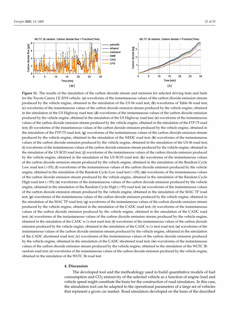
Figure 11. The results of the simulation of the carbon dioxide stream and emission for selected driving tests and fuels for the Toyota Camry LE 2018 vehicle: (a) waveforms of the instantaneous values of the carbon dioxide emission stream pro-duced by the vehicle engine, obtained in the simulation of the US 06 road test; (b) waveforms of Table 06 road test; (c) waveforms of the instantaneous values of the carbon dioxide emission stream produced by the vehicle engine, obtained in the simulation of the US Highway road test; (d) waveforms of the instantaneous values of the carbon dioxide emission produced by the vehicle engine, obtained in the simulation of the US Highway road test; (e) waveforms of the instantane-ous values of the carbon dioxide emission stream produced by the vehicle engine, obtained in the simulation of the FTP-75 road test; (f) waveforms of the instantaneous values of the carbon dioxide emission produced by the vehicle engine, obtained in the simulation of the FTP-75 road test; (g) waveforms of the instantaneous values of the carbon dioxide emis-sion stream produced by the vehicle engine, obtained in the simulation of the NEDC road test; (h) waveforms of the instantaneous values of the carbon dioxide emission produced by the vehicle engine, obtained in the simulation of the US 06 road test; (i) waveforms of the instantaneous values of the carbon dioxide emission stream produced by the vehicle engine, obtained in the simulation of the US SC03 road test; (j) waveforms of the instantaneous values of the carbon diox-ide emission produced by the vehicle engine, obtained in the simulation of the US SC03 road test; (k) waveforms of the instantaneous values of the carbon dioxide emission stream produced by the vehicle engine, obtained in the simulation of the Random Cycle Low road test (×05); (l) waveforms of the instantaneous values of the carbon dioxide emission produced by the vehicle engine, obtained in the simulation of the Random Cycle Low road test (×05); (m) waveforms of the instan-taneous values of the carbon dioxide emission stream produced by the vehicle engine, obtained in the simulation of the Random Cycle High road test (×95); (n) waveforms of the instantaneous values of the carbon dioxide emission produced by the vehicle engine, obtained in the simulation of the Random Cycle High (×95) road test; (o) waveforms of the instan-taneous values of the carbon dioxide emission stream produced by the vehicle engine, obtained in the simulation of the MAC TP road test; (p) waveforms of the instantaneous values of the carbon dioxide emission produced by the vehicle engine, obtained in the simulation of the MAC TP road test; (q) waveforms of the instantaneous values of the carbon dioxide emission stream produced by the vehicle engine, obtained in the simulation of the CADC road test; (r) waveforms of the instantaneous values of the carbon dioxide emission produced by the vehicle engine, obtained in the simulation of the CADC road test; (s) waveforms of the instantaneous values of the carbon dioxide emission stream produced by the vehicle engine, obtained in the simulation of the CADC w/o mot road test; (t) waveforms of the instantaneous values of the carbon dioxide emission produced by the vehicle engine, obtained in the simulation of the CADC w/o mot road test; (u) waveforms of the instantaneous values of the carbon dioxide emission stream produced by the vehicle engine, obtained in the simulation of the CADC shortened road test; (v) waveforms of the instantaneous values of the carbon dioxide emis-sion produced by the vehicle engine, obtained in the simulation of the CADC shortened road test; (w) waveforms of the instantaneous values of the carbon dioxide emission stream produced by the vehicle engine, obtained in the simulation of the WLTC 3b random road test; (x) waveforms of the instantaneous values of the carbon dioxide emission produced by the vehicle engine, obtained in the simulation of the WLTC 3b road test.
4. Discussion The developed tool and the methodology used to build quantitative models of fuel
consumption and CO2 emissivity of the selected vehicle as a function of engine load and vehicle speed might constitute the basis for the construction of road simulators. In this case, the simulation tool can be adapted to the operational parameters of a large set of vehicles that represent a given car market. Road simulators developed on the basis of the described tool will make it possible to obtain more precise emissivity values in road traffic than the adopted environmental estimates.
Figure 12 presents the results of the simulator work for the considered fuels and driv-ing tests in the form of the fuel consumption parameter per one kilometer driven in the test. For CNG fuel, the minimum value was achieved at the level of 32 g/km for the US
Figure 11. The results of the simulation of the carbon dioxide stream and emission for selected driving tests and fuelsfor the Toyota Camry LE 2018 vehicle: (a) waveforms of the instantaneous values of the carbon dioxide emission streamproduced by the vehicle engine, obtained in the simulation of the US 06 road test; (b) waveforms of Table 06 road test;(c) waveforms of the instantaneous values of the carbon dioxide emission stream produced by the vehicle engine, obtainedin the simulation of the US Highway road test; (d) waveforms of the instantaneous values of the carbon dioxide emissionproduced by the vehicle engine, obtained in the simulation of the US Highway road test; (e) waveforms of the instantaneousvalues of the carbon dioxide emission stream produced by the vehicle engine, obtained in the simulation of the FTP-75 roadtest; (f) waveforms of the instantaneous values of the carbon dioxide emission produced by the vehicle engine, obtained inthe simulation of the FTP-75 road test; (g) waveforms of the instantaneous values of the carbon dioxide emission streamproduced by the vehicle engine, obtained in the simulation of the NEDC road test; (h) waveforms of the instantaneousvalues of the carbon dioxide emission produced by the vehicle engine, obtained in the simulation of the US 06 road test;(i) waveforms of the instantaneous values of the carbon dioxide emission stream produced by the vehicle engine, obtained inthe simulation of the US SC03 road test; (j) waveforms of the instantaneous values of the carbon dioxide emission producedby the vehicle engine, obtained in the simulation of the US SC03 road test; (k) waveforms of the instantaneous valuesof the carbon dioxide emission stream produced by the vehicle engine, obtained in the simulation of the Random CycleLow road test (×05); (l) waveforms of the instantaneous values of the carbon dioxide emission produced by the vehicleengine, obtained in the simulation of the Random Cycle Low road test (×05); (m) waveforms of the instantaneous valuesof the carbon dioxide emission stream produced by the vehicle engine, obtained in the simulation of the Random CycleHigh road test (×95); (n) waveforms of the instantaneous values of the carbon dioxide emission produced by the vehicleengine, obtained in the simulation of the Random Cycle High (×95) road test; (o) waveforms of the instantaneous valuesof the carbon dioxide emission stream produced by the vehicle engine, obtained in the simulation of the MAC TP roadtest; (p) waveforms of the instantaneous values of the carbon dioxide emission produced by the vehicle engine, obtained inthe simulation of the MAC TP road test; (q) waveforms of the instantaneous values of the carbon dioxide emission streamproduced by the vehicle engine, obtained in the simulation of the CADC road test; (r) waveforms of the instantaneousvalues of the carbon dioxide emission produced by the vehicle engine, obtained in the simulation of the CADC roadtest; (s) waveforms of the instantaneous values of the carbon dioxide emission stream produced by the vehicle engine,obtained in the simulation of the CADC w/o mot road test; (t) waveforms of the instantaneous values of the carbon dioxideemission produced by the vehicle engine, obtained in the simulation of the CADC w/o mot road test; (u) waveforms of theinstantaneous values of the carbon dioxide emission stream produced by the vehicle engine, obtained in the simulationof the CADC shortened road test; (v) waveforms of the instantaneous values of the carbon dioxide emission producedby the vehicle engine, obtained in the simulation of the CADC shortened road test; (w) waveforms of the instantaneousvalues of the carbon dioxide emission stream produced by the vehicle engine, obtained in the simulation of the WLTC 3brandom road test; (x) waveforms of the instantaneous values of the carbon dioxide emission produced by the vehicle engine,obtained in the simulation of the WLTC 3b road test.
4. Discussion
The developed tool and the methodology used to build quantitative models of fuelconsumption and CO2 emissivity of the selected vehicle as a function of engine load andvehicle speed might constitute the basis for the construction of road simulators. In this case,the simulation tool can be adapted to the operational parameters of a large set of vehiclesthat represent a given car market. Road simulators developed on the basis of the described
Energies 2021, 14, 1400 22 of 33
tool will make it possible to obtain more precise emissivity values in road traffic than theadopted environmental estimates.
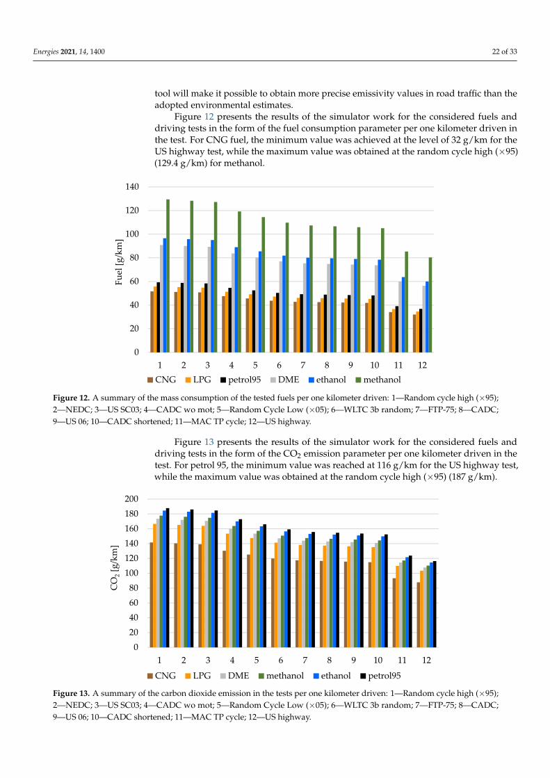
Figure 12 presents the results of the simulator work for the considered fuels anddriving tests in the form of the fuel consumption parameter per one kilometer driven inthe test. For CNG fuel, the minimum value was achieved at the level of 32 g/km for theUS highway test, while the maximum value was obtained at the random cycle high (×95)(129.4 g/km) for methanol.
Energies 2021, 14, x FOR PEER REVIEW 22 of 33
highway test, while the maximum value was obtained at the random cycle high (×95) (129.4 g/km) for methanol.
Figure 12. A summary of the mass consumption of the tested fuels per one kilometer driven: 1—Random cycle high (×95); 2—NEDC; 3—US SC03; 4—CADC wo mot; 5—Random Cycle Low (×05); 6—WLTC 3b random; 7—FTP-75; 8—CADC; 9—US 06; 10—CADC shortened; 11—MAC TP cycle; 12—US highway.
Figure 13 presents the results of the simulator work for the considered fuels and driv-ing tests in the form of the CO2 emission parameter per one kilometer driven in the test. For petrol 95, the minimum value was reached at 116 g/km for the US highway test, while the maximum value was obtained at the random cycle high (×95) (187 g/km).
Figure 13. A summary of the carbon dioxide emission in the tests per one kilometer driven: 1—Random cycle high (×95); 2—NEDC; 3—US SC03; 4—CADC wo mot; 5—Random Cycle Low (×05); 6—WLTC 3b random; 7—FTP-75; 8—CADC; 9—US 06; 10—CADC shortened; 11—MAC TP cycle; 12—US highway.
0
20
40
60
80
100
120
140
1 2 3 4 5 6 7 8 9 10 11 12
Fuel
[g/k
m]
CNG LPG petrol95 DME ethanol methanol
020406080
100120140160180200
1 2 3 4 5 6 7 8 9 10 11 12
CO
2[g
/km
]
CNG LPG DME methanol ethanol petrol95
Figure 12. A summary of the mass consumption of the tested fuels per one kilometer driven: 1—Random cycle high (×95);2—NEDC; 3—US SC03; 4—CADC wo mot; 5—Random Cycle Low (×05); 6—WLTC 3b random; 7—FTP-75; 8—CADC;9—US 06; 10—CADC shortened; 11—MAC TP cycle; 12—US highway.
Figure 13 presents the results of the simulator work for the considered fuels anddriving tests in the form of the CO2 emission parameter per one kilometer driven in thetest. For petrol 95, the minimum value was reached at 116 g/km for the US highway test,while the maximum value was obtained at the random cycle high (×95) (187 g/km).
Energies 2021, 14, x FOR PEER REVIEW 22 of 33
highway test, while the maximum value was obtained at the random cycle high (×95) (129.4 g/km) for methanol.
Figure 12. A summary of the mass consumption of the tested fuels per one kilometer driven: 1—Random cycle high (×95); 2—NEDC; 3—US SC03; 4—CADC wo mot; 5—Random Cycle Low (×05); 6—WLTC 3b random; 7—FTP-75; 8—CADC; 9—US 06; 10—CADC shortened; 11—MAC TP cycle; 12—US highway.
Figure 13 presents the results of the simulator work for the considered fuels and driv-ing tests in the form of the CO2 emission parameter per one kilometer driven in the test. For petrol 95, the minimum value was reached at 116 g/km for the US highway test, while the maximum value was obtained at the random cycle high (×95) (187 g/km).
Figure 13. A summary of the carbon dioxide emission in the tests per one kilometer driven: 1—Random cycle high (×95); 2—NEDC; 3—US SC03; 4—CADC wo mot; 5—Random Cycle Low (×05); 6—WLTC 3b random; 7—FTP-75; 8—CADC; 9—US 06; 10—CADC shortened; 11—MAC TP cycle; 12—US highway.
0
20
40
60
80
100
120
140
1 2 3 4 5 6 7 8 9 10 11 12
Fuel
[g/k
m]
CNG LPG petrol95 DME ethanol methanol
020406080
100120140160180200
1 2 3 4 5 6 7 8 9 10 11 12
CO
2[g
/km
]
CNG LPG DME methanol ethanol petrol95
Figure 13. A summary of the carbon dioxide emission in the tests per one kilometer driven: 1—Random cycle high (×95);2—NEDC; 3—US SC03; 4—CADC wo mot; 5—Random Cycle Low (×05); 6—WLTC 3b random; 7—FTP-75; 8—CADC;9—US 06; 10—CADC shortened; 11—MAC TP cycle; 12—US highway.
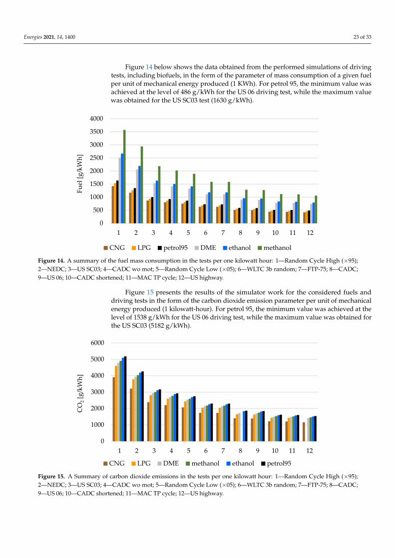
Energies 2021, 14, 1400 23 of 33
Figure 14 below shows the data obtained from the performed simulations of drivingtests, including biofuels, in the form of the parameter of mass consumption of a given fuelper unit of mechanical energy produced (1 KWh). For petrol 95, the minimum value wasachieved at the level of 486 g/kWh for the US 06 driving test, while the maximum valuewas obtained for the US SC03 test (1630 g/kWh).
Energies 2021, 14, x FOR PEER REVIEW 23 of 33
Figure 14 below shows the data obtained from the performed simulations of driving tests, including biofuels, in the form of the parameter of mass consumption of a given fuel per unit of mechanical energy produced (1 KWh). For petrol 95, the minimum value was achieved at the level of 486 g/kWh for the US 06 driving test, while the maximum value was obtained for the US SC03 test (1630 g/kWh).
Figure 14. A summary of the fuel mass consumption in the tests per one kilowatt hour: 1—Ran-dom Cycle High (×95); 2—NEDC; 3—US SC03; 4—CADC wo mot; 5—Random Cycle Low (×05); 6—WLTC 3b random; 7—FTP-75; 8—CADC; 9—US 06; 10—CADC shortened; 11—MAC TP cycle; 12—US highway.
Figure 15 presents the results of the simulator work for the considered fuels and driv-ing tests in the form of the carbon dioxide emission parameter per unit of mechanical en-ergy produced (1 kilowatt-hour). For petrol 95, the minimum value was achieved at the level of 1538 g/kWh for the US 06 driving test, while the maximum value was obtained for the US SC03 (5182 g/kWh).
Figure 15. A Summary of carbon dioxide emissions in the tests per one kilowatt hour: 1—Random Cycle High (×95); 2—NEDC; 3—US SC03; 4—CADC wo mot; 5—Random Cycle Low (×05); 6—WLTC 3b random; 7—FTP-75; 8—CADC; 9—US 06; 10—CADC shortened; 11—MAC TP cycle; 12—US highway.
0
500
1000
1500
2000
2500
3000
3500
4000
1 2 3 4 5 6 7 8 9 10 11 12
Fuel
[g/k
Wh]
CNG LPG petrol95 DME ethanol methanol
0
1000
2000
3000
4000
5000
6000
1 2 3 4 5 6 7 8 9 10 11 12
CO
2[g
/kW
h]
CNG LPG DME methanol ethanol petrol95
Figure 14. A summary of the fuel mass consumption in the tests per one kilowatt hour: 1—Random Cycle High (×95);2—NEDC; 3—US SC03; 4—CADC wo mot; 5—Random Cycle Low (×05); 6—WLTC 3b random; 7—FTP-75; 8—CADC;9—US 06; 10—CADC shortened; 11—MAC TP cycle; 12—US highway.
Figure 15 presents the results of the simulator work for the considered fuels anddriving tests in the form of the carbon dioxide emission parameter per unit of mechanicalenergy produced (1 kilowatt-hour). For petrol 95, the minimum value was achieved at thelevel of 1538 g/kWh for the US 06 driving test, while the maximum value was obtained forthe US SC03 (5182 g/kWh).
Energies 2021, 14, x FOR PEER REVIEW 23 of 33
Figure 14 below shows the data obtained from the performed simulations of driving tests, including biofuels, in the form of the parameter of mass consumption of a given fuel per unit of mechanical energy produced (1 KWh). For petrol 95, the minimum value was achieved at the level of 486 g/kWh for the US 06 driving test, while the maximum value was obtained for the US SC03 test (1630 g/kWh).
Figure 14. A summary of the fuel mass consumption in the tests per one kilowatt hour: 1—Ran-dom Cycle High (×95); 2—NEDC; 3—US SC03; 4—CADC wo mot; 5—Random Cycle Low (×05); 6—WLTC 3b random; 7—FTP-75; 8—CADC; 9—US 06; 10—CADC shortened; 11—MAC TP cycle; 12—US highway.
Figure 15 presents the results of the simulator work for the considered fuels and driv-ing tests in the form of the carbon dioxide emission parameter per unit of mechanical en-ergy produced (1 kilowatt-hour). For petrol 95, the minimum value was achieved at the level of 1538 g/kWh for the US 06 driving test, while the maximum value was obtained for the US SC03 (5182 g/kWh).
Figure 15. A Summary of carbon dioxide emissions in the tests per one kilowatt hour: 1—Random Cycle High (×95); 2—NEDC; 3—US SC03; 4—CADC wo mot; 5—Random Cycle Low (×05); 6—WLTC 3b random; 7—FTP-75; 8—CADC; 9—US 06; 10—CADC shortened; 11—MAC TP cycle; 12—US highway.
0
500
1000
1500
2000
2500
3000
3500
4000
1 2 3 4 5 6 7 8 9 10 11 12
Fuel
[g/k
Wh]
CNG LPG petrol95 DME ethanol methanol
0
1000
2000
3000
4000
5000
6000
1 2 3 4 5 6 7 8 9 10 11 12
CO
2[g
/kW
h]
CNG LPG DME methanol ethanol petrol95
Figure 15. A Summary of carbon dioxide emissions in the tests per one kilowatt hour: 1—Random Cycle High (×95);2—NEDC; 3—US SC03; 4—CADC wo mot; 5—Random Cycle Low (×05); 6—WLTC 3b random; 7—FTP-75; 8—CADC;9—US 06; 10—CADC shortened; 11—MAC TP cycle; 12—US highway.
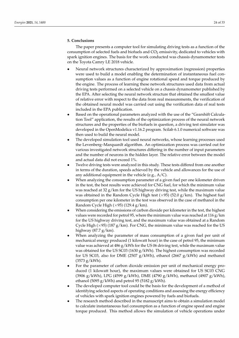
Energies 2021, 14, 1400 24 of 33
5. Conclusions
The paper presents a computer tool for simulating driving tests as a function of theconsumption of selected fuels and biofuels and CO2 emissivity, dedicated to vehicles withspark ignition engines. The basis for the work conducted was chassis dynamometer testson the Toyota Camry LE 2018 vehicle.
• Neural network structures characterized by approximation (regression) propertieswere used to build a model enabling the determination of instantaneous fuel con-sumption values as a function of engine rotational speed and torque produced bythe engine. The process of learning these network structures used data from actualdriving tests performed on a selected vehicle on a chassis dynamometer published bythe EPA. After selecting the neural network structure that obtained the smallest valueof relative error with respect to the data from real measurements, the verification ofthe obtained neural model was carried out using the verification data of real testsincluded in the EPA publication.
• Based on the operational parameters analyzed with the use of the “Gearshift Calcula-tion Tool” application, the results of the optimization process of the neural networkstructures and the properties of the biofuels in question, a driving test simulator wasdeveloped in the OpenModelica v1.16.2 program. Scilab 6.1.0 numerical software wasthen used to build the neural model.
• The developed simulation tool used neural networks, whose learning processes usedthe Levenberg–Marquardt algorithm. An optimization process was carried out forvarious investigated network structures differing in the number of input parametersand the number of neurons in the hidden layer. The relative error between the modeland actual data did not exceed 1%.
• Twelve driving tests were analyzed in this study. These tests differed from one anotherin terms of the duration, speeds achieved by the vehicle and allowances for the use ofany additional equipment in the vehicle (e.g., A/C).
• When analyzing the consumption parameter of a given fuel per one kilometer drivenin the test, the best results were achieved for CNG fuel, for which the minimum valuewas reached at 32 g/km for the US highway driving test, while the maximum valuewas obtained in the Random Cycle High test (×95) (52.0 g/km). The highest fuelconsumption per one kilometer in the test was observed in the case of methanol in theRandom Cycle High (×95) (129.4 g/km).
• When considering the emissions of carbon dioxide per kilometer in the test, the highestvalues were recorded for petrol 95, where the minimum value was reached at 116 g/kmfor the US highway driving test, and the maximum value was obtained at a RandomCycle High (×95) (187 g/km). For CNG, the minimum value was reached for the UShighway (87.7 g/km).
• When analyzing the parameter of mass consumption of a given fuel per unit ofmechanical energy produced (1 kilowatt hour) in the case of petrol 95, the minimumvalue was achieved at 486 g/kWh for the US 06 driving test, while the maximum valuewas obtained for the US SC03 (1630 g/kWh). The highest consumption was recordedfor US SC03, also for DME (2507 g/kWh), ethanol (2667 g/kWh) and methanol(3573 g/kWh).
• For the parameter of carbon dioxide emission per unit of mechanical energy pro-duced (1 kilowatt hour), the maximum values were obtained for US SC03 CNG(3906 g/kWh), LPG (4599 g/kWh), DME (4790 g/kWh), methanol (4907 g/kWh),ethanol (5095 g/kWh) and petrol 95 (5182 g/kWh).
• The developed computer tool could be the basis for the development of a method ofidentifying selected aspects of operating conditions and assessing the energy efficiencyof vehicles with spark ignition engines powered by fuels and biofuels.
• The research method described in the manuscript aims to obtain a simulation modelto calculate instantaneous fuel consumption as a function of engine speed and enginetorque produced. This method allows the simulation of vehicle operations under
Energies 2021, 14, 1400 25 of 33
different load conditions and will potentially allow the calculation of fuel consumptionand carbon emissions. This method can be used for many popular vehicle models ina given market. In the case of estimating carbon dioxide emissions for real facilitieswhere vehicles move, e.g., road tunnels and large parking lots, a very large numberof simulations of individual vehicles in real traffic can be used in a single simulation.The use of such simulations will allow for the more precise selection of ventilationsystems for such objects, which will prevent the increase in carbon dioxide content inthe air.
Funding: The APC was funded by Institute of Mechanical Engineering, Warsaw University ofLife Sciences.
Institutional Review Board Statement: Not applicable.
Informed Consent Statement: Not applicable.
Data Availability Statement: All data are presented in this article. Data sharing is not applicable tothis article.
Conflicts of Interest: The author declares no conflict of interests.
References1. Beaudet, A.; Larouche, F.; Amouzegar, K.; Bouchard, P.; Zaghib, K. Key Challenges and Opportunities for Recycling Electric
Vehicle Battery Materials. Sustainability 2020, 12, 5837. [CrossRef]2. Krysko, A.V.; Awrejcewicz, J.; Pavlov, S.P.; Bodyagina, K.S.; Krysko, V.A. Topological optimization of thermoelastic composites
with maximized stiffness and heat transfer. Compos. Part B Eng. 2019, 158, 319–327. [CrossRef]3. Pawełko, P.; Berczynski, S.; Grzadziel, Z. Modeling roller guides with preload. Arch. Civ. Mech. Eng. 2014, 14, 691–699. [CrossRef]4. Nabagło, T.; Kowal, J.; Jurkiewicz, A. High Fidelity Model Construction and Its Verification Based on 2S1 Tracked Vehicle. In
Innovative Control Systems for Tracked Vehicle Platforms. Studies in Systems, Decision and Control. Part III: Construction and Investigationof the Dynamic Characteristics of Tracked Vehicles, 1st ed.; Nawrat, M.A., Ed.; Springer: Cham, Switzerland, 2015; Volume 2,pp. 205–215.
5. Maizak, D.; Wilberforce, T.; Olabi, A.G. DeNOx removal techniques for automotive applications—A review. Environ. Adv. 2020, 2,100021. [CrossRef]
6. Ogunkunle, O.; Ahmed, N.A. Exhaust emissions and engine performance analysis of a marine diesel engine fuelledwith Parinaripolyandra biodiesel–diesel blends. Energy Rep. 2020, 6, 2999–3007. [CrossRef]
7. Olabi, A.G.; Wilberforce, T.; Abdelkareem, M.A. Fuel cell application in the automotive industry and future perspective. Energy2021, 214, 118955. [CrossRef]
8. Kumar, M.S.; Prabhahar, M.; Sendilvelan, S.; Singh, S.; Venkatesh, R.; Bhaskar, K. Combustion, performance and emission analysisof a diesel engine fueled with methyl esters of Jatropha and fish oil with exhaust gas recirculation. Energy Procedia 2019, 160,404–411. [CrossRef]
9. Ang, J.G.; Fredriksson, P.G. Does an early start help or hurt? Statehood, institutions and modern climate change policies. EnergyEcon. 2021, 94, 105075. [CrossRef]
10. Fekete, H.; Kuramochi, T.; Roelfsema, M.; Den Elzen, M.; Forsell, N.; Höhne, N.; Luna, L.; Hans, F.; Sterl, S.; Olivier, J.; et al.A review of successful climate change mitigation policies in major emitting economies and the potential of global replication.Renew. Sustain. Energy Rev. 2021, 137, 110602. [CrossRef]
11. Enzmann, J.; Ringel, M. Reducing Road Transport Emissions in Europe: Investigating A Demand Side Driven Approach †.Sustainability 2020, 12, 7594. [CrossRef]
12. Coelho, S.; Rafael, S.; Lopes, D.; Miranda, A.I.; Ferreira, J. How changing climate may influence air pollution control strategies for2030? Sci. Total Environ. 2021, 758, 143911. [CrossRef]
13. Brodny, J.; Tutak, M. The analysis of similarities between the European Union countries in terms of the level and structure of theemissions of selected gases and air pollutants into the atmosphere. J. Clean. Prod. 2021, 279, 123641. [CrossRef] [PubMed]
14. Nikas, A.; Gambhir, A.; Trutnevyte, E.; Koasidis, K.; Lund, H.; Thellufsen, J.Z.; Mayer, D.; Zachmann, G.; Miguel, L.J.; Ferreras-Alonso, N.; et al. Perspective of comprehensive and comprehensible multi-model energy and climate science in Europe. Energy2021, 215, 119153. [CrossRef]
15. Cadillo-Benalcazar, J.J.; Bukkens, S.G.F.; Ripa, M.; Giampietro, M. Why does the European Union produce biofuels? Examiningconsistency and plausibility in prevailing narratives with quantitative storytelling. Energy Res. Soc. Sci. 2021, 71, 101810.[CrossRef]
16. CO2 Emissions from Cars: Facts and Figures (Infographics). Available online: https://www.europarl.europa.eu/news/en/headlines/society/20190313STO31218/co2-emissions-from-cars-facts-and-figures-infographics (accessed on 23 January 2021).
Energies 2021, 14, 1400 26 of 33
17. McKinsey & Company. Carbon-Neutral Poland 2050. Available online: https://www.mckinsey.com/pl/our-insights/carbon-neutral-poland-2050 (accessed on 23 January 2021).
18. European Parliament Approves Post-2020 CO2 Emission Targets for Cars and Vans. Available online: https://ihsmarkit.com/research-analysis/european-parliament-approves-post2020-co2-emission-targets.html (accessed on 23 January 2021).
19. AECC Newsletter March 2019. Available online: https://www.aecc.eu/wp-content/uploads/2019/04/AECC-Newsletter-March-2019.pdf (accessed on 23 January 2021).
20. Transport. Available online: https://www.ipcc.ch/site/assets/uploads/2018/02/ipcc_wg3_ar5_chapter8.pdf (accessed on23 January 2021).
21. Jing, R.; Yuan, C.; Rezaei, H.; Qian, J.; Zhang, Z. Assessments on emergy and greenhouse gas emissions of internal combustionengine automobiles and electric automobiles in the USA. J. Environ. Sci. 2020, 90, 297–309. [CrossRef] [PubMed]
22. Akhshik, M.; Panthapulakkal, S.; Tjong, J.; Bilton, A.; Singh, C.V.; Sain, M. Cross-country analysis of life cycle assessment–basedgreenhouse gas emissions for automotive parts: Evaluation of coefficient of country. Renew. Sustain. Energy Rev. 2021, 138, 110546.[CrossRef]
23. Daziano, R.; Waygood, E.O.D.; Patterson, Z.; Feinberg, M.; Wang, B. Reframing greenhouse gas emissions information presentationon the Environmental Protection Agency’s new-vehicle labels to increase willingness to pay. J. Clean. Prod. 2021, 279, 123669.[CrossRef]
24. Neupane, B.; Rubin, J. Implications of U.S. biofuels policy for sustainable transportation energy in Maine and the Northeast.Renew. Sustain. Energy Rev. 2017, 70, 729–735. [CrossRef]
25. Fast Facts on Transportation Greenhouse Gas Emissions. Available online: https://www.epa.gov/greenvehicles/fast-facts-transportation-greenhouse-gas-emissions (accessed on 23 January 2021).
26. Shahiduzzaman, M.; Layton, A. Decomposition analysis for assessing the United States 2025 emissions target: How big is thechallenge? Renew. Sustain. Energy Rev. 2017, 67, 372–383. [CrossRef]
27. An Overview of Automotive Vehicle and Component Regulations in China. Available online: https://incompliancemag.com/article/an-overview-of-automotive-vehicle-and-component-regulations-in-china/ (accessed on 23 January 2021).
28. Yan, X.; Crookes, R.J. Energy demand and emissions from road transportation vehicles in China. Prog. Energy Combust. Sci. 2010,36, 651–676. [CrossRef]
29. Liu, Y.; Wu, Z.X.; Zhou, H.; Zheng, H.; Yu, N.; An, X.P.; Li, J.Y.; Li, M.L. Development of China Light-Duty Vehicle Test Cycle. Int.J. Automot. Technol. 2020, 21, 1233–1246. [CrossRef]
30. Liu, Y.; Zhou, H.; Xu, Y.; Qin, K.; Yu, H. Feasibility Study of Using WLTC for Fuel Consumption Certification of Chinese Light-DutyVehicles; SAE Technical Paper 2018-01-0654; SAE International: Warrendale, PA, USA, 2018.
31. Wei, L.; Li, H.; Zhang, H.; Sun, S. The Analysis of CO2 Emissions and Reduction Potential in China’s Transport Sector. Mathemat-ical Problems in Engineering. 2016, p. 1043717. Available online: https://www.hindawi.com/journals/mpe/2016/1043717/(accessed on 23 January 2021).
32. Zheng, Y.; Li, S.; Xu, S. Transport Oil Product Consumption and GHG Emission Reduction Potential in China: An ElectricVehicle-Based Scenario Analysis. Available online: https://journals.plos.org/plosone/article?id=10.1371/journal.pone.0222448(accessed on 23 January 2021).
33. Sustainable Transport in China. Available online: https://www.sustainabletransport.org/archives/tag/carbon-emissions(accessed on 23 January 2021).
34. Li, X.; Yu, B. Peaking CO2 emissions for China’s urban passenger transport sector. Energy Policy 2019, 133, 110913. [CrossRef]35. Borucka, A.; Wisniowski, P.; Mazurkiewicz, D.; Swiderski, A. Laboratory measurements of vehicle exhaust emissions in conditions
reproducing real traffic. Measurement 2021, 174, 108998. [CrossRef]36. Gao, J.; Chen, H.; Li, Y.; Chen, J.; Zhang, Y.; Dave, K.; Huang, Y. Fuel consumption and exhaust emissions of diesel vehicles in
worldwide harmonized light vehicles test cycles and their sensitivities to eco-driving factors. Energy Convers. Manag. 2019, 196,605–613. [CrossRef]
37. Sarkan, B.; Stopka, O.; Gnap, J.; Caban, J. Investigation of Exhaust Emissions of Vehicles with the Spark Ignition Engine withinEmission Control. Procedia Eng. 2017, 187, 775–782. [CrossRef]
38. Xing, J.; Shao, L.; Zhang, W.; Peng, J.; Wang, W.; Hou, C.; Shuai, S.; Hu, M.; Zhang, D. Morphology and composition of particlesemitted from a port fuel injection gasoline vehicle under real-world driving test cycles. J. Environ. Sci. 2019, 76, 339–348.[CrossRef] [PubMed]
39. Koossalapeerom, T.; Satiennam, T.; Satiennam, W.; Leelapatra, W.; Seedam, A.; Rakpukdee, T. Comparative study of real-worlddriving cycles, energy consumption, and CO2 emissions of electric and gasoline motorcycles driving in a congested urbancorridor. Sustain. Cities Soc. 2019, 45, 619–627. [CrossRef]
40. Wang, Y.; Hao, C.; Ge, Y.; Hao, L.; Tan, J.; Wang, X.; Zhang, P.; Wang, Y.; Tian, W.; Lin, Z.; et al. Fuel consumption and emissionperformance from light-duty conventional/hybrid-electric vehicles over different cycles and real driving tests. Fuel 2020, 278,118340. [CrossRef]
41. Hagino, H.; Oyama, M.; Sasaki, S. Laboratory testing of airborne brake wear particle emissions using a dynamometer systemunder urban city driving cycles. Atmos. Environ. 2016, 131, 269–278. [CrossRef]
Energies 2021, 14, 1400 27 of 33
42. Wihersaari, H.; Pirjola, L.; Karjalainen, P.; Saukko, E.; Kuuluvainen, H.; Kulmala, K.; Keskinen, J.; Rönkkö, T. Particulate emissionsof a modern diesel passenger car under laboratory and real-world transient driving conditions. Environ. Pollut. 2020, 265, 114948.[CrossRef]
43. Davari, M.M.; Jerrelind, J.; Trigell, A.S. Energy efficiency analyses of a vehicle in modal and transient driving cycles includinglongitudinal and vertical dynamics. Transp. Res. Part D Transp. Environ. 2017, 53, 263–275. [CrossRef]
44. Triantafyllopoulos, G.; Dimaratos, A.; Ntziachristos, L.; Bernard, Y.; Dornoff, J.; Samaras, Z. A study on the CO2 and NOxemissions performance of Euro 6 diesel vehicles under various chassis dynamometer and on-road conditions including latestregulatory provisions. Sci. Total Environ. 2019, 666, 337–346. [CrossRef]
45. Chen, L.; Wang, Z.; Liu, S.; Qu, L. Using a chassis dynamometer to determine the influencing factors for the emissions of Euro VIvehicles. Transp. Res. Part D Transp. Environ. 2018, 65, 564–573. [CrossRef]
46. Lohse-Busch, H.; Stutenberg, K.; Duoba, M.; Liu, X.; Elgowainy, A.; Wang, M.; Wallner, T.; Richard, B.; Christenson, M. Automotivefuel cell stack and system efficiency and fuel consumption based on vehicle testing on a chassis dynamometer at minus 18 ◦C topositive 35 ◦C temperatures. Int. J. Hydrogen Energy 2020, 45, 861–872. [CrossRef]
47. Zhu, G.; Liu, F.J.; Xu, Z.; Guo, Q.; Zhao, H. Experimental study on combustion and emission characteristics of turbochargedgasoline direct injection (GDI) engine under cold start new European driving cycle (NEDC). Fuel 2015, 215, 272–284. [CrossRef]
48. Armas, O.; García-Contreras, R.; Ramos, A. Pollutant emissions from New European Driving Cycle with ethanol and butanoldiesel blends. Fuel Process. Technol. 2014, 122, 64–71. [CrossRef]
49. Degraeuwe, B.; Weiss, M. Does the New European Driving Cycle (NEDC) really fail to capture the NOX emissions of diesel carsin Europe? Environ. Pollut. 2017, 222, 234–241. [CrossRef] [PubMed]
50. Ramos, A.; Muñoz, J.; Andrés, F.; Armas, O. NOx emissions from diesel light duty vehicle tested under NEDC and real-worddriving conditions. Transp. Res. Part D Transp. Environ. 2018, 63, 37–48. [CrossRef]
51. Fontaras, G.; Valverde, V.; Arcidiacono, V.; Tsiakmakis, S.; Anagnostopoulos, K.; Komnos, D.; Pavlovic, J.; Ciuffo, B. Thedevelopment and validation of a vehicle simulator for the introduction of Worldwide Harmonized test protocol in the Europeanlight duty vehicle CO2 certification process. Appl. Energy 2018, 226, 784–796. [CrossRef]
52. Tsiakmakis, S.; Fontaras, G.; Anagnostopoulos, K.; Ciuffo, B.; Pavlovic, J.; Marotta, A. A simulation based approach forquantifying CO2 emissions of light duty vehicle fleets. A case study on WLTP introduction. Transp. Res. Procedia 2017, 25,3898–3908. [CrossRef]
53. Massaguer, E.; Massaguer, A.; Pujol, T.; Comamala, M.; Montoro, L.; Gonzalez, J.R. Fuel economy analysis under a WLTP cycle ona mid-size vehicle equipped with a thermoelectric energy recovery system. Energy 2019, 179, 306–314. [CrossRef]
54. The Introduction of the WLTP into the European Type-Approval for Light-Duty Vehicles. Available online: https://ec.europa.eu/jrc/sites/jrcsh/files/wltp_20oct-morning_1.pdf (accessed on 27 January 2021).
55. Tutuianu, M.; Bonnel, P.; Ciuffo, B.; Haniu, T.; Ichikawa, N.; Marotta, A.; Pavlovic, J.; Steven, H. Development of the World-wideharmonized Light duty Test Cycle (WLTC) and a possible pathway for its introduction in the European legislation. Transp. Res.Part D Transp. Environ. 2015, 40, 61–75. [CrossRef]
56. Dimaratos, A.; Tsokolis, D.; Fontaras, G.; Tsiakmakis, S.; Ciuffo, B.; Samaras, Z. Comparative Evaluation of the Effect of VariousTechnologies on Light-duty Vehicle CO2 Emissions over NEDC and WLTP. Transp. Res. Procedia 2016, 14, 3169–3178. [CrossRef]
57. Duarte, G.O.; Gonçalves, G.A.; Farias, T.L. Analysis of fuel consumption and pollutant emissions of regulated and alternativedriving cycles based on real-world measurements. Transp. Res. Part D Transp. Environ. 2016, 44, 43–54. [CrossRef]
58. From NEDC to WLTP: What Will Change? Available online: https://www.wltpfacts.eu/from-nedc-to-wltp-change/ (accessedon 27 January 2021).
59. Abdelkareem, M.A.A.; Xu, L.; Guo, X.; Ali, M.K.A.; Elagouz, A.; Hassan, M.A.; Essa, F.A.; Zou, J. Energy harvesting sensitivityanalysis and assessment of the potential power and full car dynamics for different road modes. Mech. Syst. Signal Process. 2018,110, 307–332. [CrossRef]
60. Björnsson, L.H.; Karlsson, S. The potential for brake energy regeneration under Swedish conditions. Appl. Energy 2016, 168, 75–84.[CrossRef]
61. Global WLTP Roll-Out for More Realistic Results in Fuel Consumption. Available online: https://www.vda.de/en/topics/environment-and-climate/Global-WLTP-roll-out-for-more-realistic-results-in-fuel-consumption/WLTP-How-realistic-is-the-WLTP.html (accessed on 27 January 2021).
62. WLTP Driving Cycle. Available online: https://www.vauxhall.co.uk/wltp.html (accessed on 27 January 2021).63. Wang, S.; Li, Y.; Fu, J.; Liu, J.; Dong, H. Numerical research on the performance, combustion and energy flow characteristics of
gasoline-powered vehicle under WLTC. Fuel 2021, 285, 119135. [CrossRef]64. Karagöz, Y. Analysis of the impact of gasoline, biogas and biogas + hydrogen fuels on emissions and vehicle performance in the
WLTC and NEDC. Int. J. Hydrogen Energy 2019, 44, 31621–31632. [CrossRef]65. Sileghem, L.; Bosteels, D.; May, J.; Favre, C.; Verhelst, S. Analysis of vehicle emission measurements on the new WLTC, the NEDC
and the CADC. Transp. Res. Part D Transp. Environ. 2014, 32, 70–85. [CrossRef]66. Zachiotis, A.T.; Giakoumis, E.G. Non-regulatory parameters effect on consumption and emissions from a diesel-powered van
over the WLTC. Transp. Res. Part D Transp. Environ. 2019, 74, 104–123. [CrossRef]67. Wang, Y.; Ge, Y.; Wang, J.; Wang, X.; Yin, H.; Hao, L.; Tan, J. Impact of altitude on the real driving emission (RDE) results
calculated in accordance to moving averaging window (MAW) method. Fuel 2020, 277, 117929. [CrossRef]
Energies 2021, 14, 1400 28 of 33
68. Kurtyka, K.; Pielecha, J. The evaluation of exhaust emission in RDE tests including dynamic driving conditions. Transp. Res.Procedia 2019, 40, 338–345. [CrossRef]
69. García-Contreras, R.; Soriano, J.A.; Fernández-Yáñez, P.; Sánchez-Rodríguez, L.; Mata, C.; Gómez, A.; Armas, O.; Cárdenas, M.D.Impact of regulated pollutant emissions of Euro 6d-Temp light-duty diesel vehicles under real driving conditions. J. Clean. Prod.2021, 286, 124927. [CrossRef]
70. Expectations for Actual Euro 6 Vehicle Emissions. Available online: https://www.concawe.eu/publication/expectations-actual-euro-6-vehicle-emissions/ (accessed on 27 January 2021).
71. Park, J.; Shin, M.; Lee, J.; Lee, J. Estimating the effectiveness of vehicle emission regulations for reducing NOx from light-dutyvehicles in Korea using on-road measurements. Sci. Total Environ. 2021, 767, 144250. [CrossRef]
72. Triantafyllopoulos, G.; Katsaounis, D.; Karamitros, D.; Ntziachristos, L.; Samaras, Z. Experimental assessment of the potential todecrease diesel NOx emissions beyond minimum requirements for Euro 6 Real Drive Emissions (RDE) compliance. Sci. TotalEnviron. 2018, 618, 1400–1407. [CrossRef]
73. Du, B.; Zhang, L.; Geng, Y.; Zhang, Y.; Xu, H.; Xiang, G. Testing and evaluation of cold-start emissions in a real driving emissionstest. Transp. Res. Part D Transp. Environ. 2020, 86, 102447. [CrossRef]
74. Yang, Z.; Ge, Y.; Thomas, D.; Wang, X.; Su, S.; Li, H.; He, H. Real driving particle number (PN) emissions from China-6 compliantPFI and GDI hybrid electrical vehicles. Atmos. Environ. 2019, 199, 70–79. [CrossRef]
75. Varella, R.A.; Faria, M.V.; Mendoza-Villafuerte, P.; Baptista, P.C.; Sousa, L.; Duarte, G.O. Assessing the influence of boundaryconditions, driving behavior and data analysis methods on real driving CO2 and NOx emissions. Sci. Total Environ. 2019, 658,879–894. [CrossRef] [PubMed]
76. Lenz, M.; Hoehl, T.; Zanger, L.; Pischinger, S. Approach to determine the entropy coefficient of a battery by numerical optimization.J. Power Sources 2020, 480, 228841. [CrossRef]
77. Chindamo, D.; Gadola, M. What is the Most Representative Standard Driving Cycle to Estimate Diesel Emissions of a LightCommercial Vehicle? IFAC-PapersOnLine 2018, 51, 73–78. [CrossRef]
78. Napolitano, P.; Guido, C.; Beatrice, C.; Pellegrini, L. Impact of hydrocracked diesel fuel and Hydrotreated Vegetable Oil blends onthe fuel consumption of automotive diesel engines. Fuel 2018, 222, 718–732. [CrossRef]
79. Scaradozzi, D.; Fanesi, M. Advanced Control Strategies to Improve Nonlinear Automotive Dynamical Systems Consumption.Axioms 2019, 8, 123. [CrossRef]
80. Institute of Internal Combustion Engines and Thermodynamics. Measurement of CO2- and Fuel Consumption from Cars in theNEDC and in Real-World-Driving Cycles. Available online: https://ermes-group.eu/web/system/files/filedepot/9/2009-TUG-NEDC-real-world-CO2.pdf (accessed on 28 January 2021).
81. Association for Emissions Control by Catalyst (AECC). Particulate Emissions from Typical Light-Duty Vehicles Taken from theEuropean Fleet, Equipped with a Variety of Emissions Control Technologies. Available online: https://www.nanoparticles.ch/archive/2011_May_PR.pdf (accessed on 28 January 2021).
82. The Mobile Air-Conditioning Systems MACs. Available online: https://ec.europa.eu/growth/sectors/automotive/environment-protection/mobile-air-conditioning-systems_en (accessed on 28 January 2021).
83. Li, C.; Brewer, E.; Pham, L.; Jung, H. Reducing Mobile Air Conditioner (MAC) Power Consumption Using Active Cabin-Air-Recirculation in A Plug-In Hybrid Electric Vehicle (PHEV). World Electr. Veh. J. 2018, 9, 51. [CrossRef]
84. Shendge, S.; Tilekar, P.; Dahiya, S.; Kapoor, S. Reduction of MAC Power Requirement in a Small Car; 2010-01-0803; SAE International:Warrendale, PA, USA, 2010.
85. Monforte, R.; Lovuolo, F.; Rostagno, M.; Seccardini, R. New MAC Technologies: Fuel Efficiency Effect in Real Driving of the Air IntakeFlap Management; 2015-01-1609; SAE International: Warrendale, PA, USA, 2015.
86. Sciance, F.; Nelson, B.; Yassine, M.; Patti, A.; Rao, L. Developing the AC17 Efficiency Test for Mobile Air Conditioners; 2013-01-0569;SAE International: Warrendale, PA, USA, 2013.
87. Kim, J.; Choi, K.; Myung, C.L.; Lee, Y.; Park, S. Comparative investigation of regulated emissions and nano-particle characteristicsof light duty vehicles using various fuels for the FTP-75 and the NEDC mode. Fuel 2013, 106, 335–343. [CrossRef]
88. Zhang, C.; Miller, E.; Kotz, A.; Kelly, K.; Thornton, M.; Geller, M.; Brezny, R. Characterization of commercial vehicles’ start-upoperations from in-use data. Transp. Res. Part D Transp. Environ. 2021, 91, 102694. [CrossRef]
89. Myung, C.L.; Jang, W.; Kwon, S.; Ko, J.; Jin, D.; Park, S. Evaluation of the real-time de-NOx performance characteristics ofa LNT-equipped Euro-6 diesel passenger car with various vehicle emissions certification cycles. Energy 2017, 132, 356–369.[CrossRef]
90. Myung, C.L.; Choi, K.; Kim, J.; Lim, Y.; Lee, J.; Park, S. Comparative study of regulated and unregulated toxic emissionscharacteristics from a spark ignition direct injection light-duty vehicle fueled with gasoline and liquid phase LPG (liquefiedpetroleum gas). Energy 2012, 44, 189–196. [CrossRef]
91. Roso, V.R.; Santos, N.D.S.A.; Valle, R.M.; Alvarez, C.E.C.; Monsalve-Serrano, J.; García, A. Evaluation of a stratified prechamberignition concept for vehicular applications in real world and standardized driving cycles. Appl. Energy 2019, 254, 113691.[CrossRef]
92. Benajes, J.; García, A.; Monsalve-Serrano, J.; Sari, R.L. Fuel consumption and engine-out emissions estimations of a light-dutyengine running in dual-mode RCCI/CDC with different fuels and driving cycles. Energy 2018, 157, 19–30. [CrossRef]
Energies 2021, 14, 1400 29 of 33
93. Kim, J.; Kim, K.; Oh, S. An assessment of the ultra-lean combustion direct-injection LPG (liquefied petroleum gas) engine forpassenger-car applications under the FTP-75 mode. Fuel Process. Technol. 2016, 154, 219–226. [CrossRef]
94. Jhang, S.R.; Lin, Y.C.; Chen, K.S.; Lin, S.L.; Batterman, S. Evaluation of fuel consumption, pollutant emissions and well-to-wheelGHGs assessment from a vehicle operation fueled with bioethanol, gasoline and hydrogen. Energy 2020, 209, 118436. [CrossRef]
95. Hu, Z.; Lu, Z.; Song, B.; Quan, Y. Impact of test cycle on mass, number and particle size distribution of particulates emitted fromgasoline direct injection vehicles. Sci. Total Environ. 2021, 762, 143128. [CrossRef] [PubMed]
96. Supplemental Federal Test Procedures; Overview. Available online: https://www.govregs.com/regulations/expand/title40_chapterI-i36_part1066_subpartI_section1066.830 (accessed on 29 January 2021).
97. Lee, J.S. Stability Analysis of Deadbeat-Direct Torque and Flux Control for Permanent Magnet Synchronous Motor Drives withRespect to Parameter Variations. Energies 2018, 11, 2027. [CrossRef]
98. Rask, E.; Bocci, D.; Duoba, M.; Lohse-Busch, H. Model Year 2010 Ford Fusion Level-1 Testing Report. Available online:https://www.osti.gov/biblio/993395-model-year-ford-fusion-level-testing-report (accessed on 29 January 2021).
99. Continental. Worldwide Emission Standards and Related Regulations. Passenger Cars/Light and Medium Duty Vehicles May2019. Available online: https://www.continental-automotive.com/getattachment/8f2dedad-b510-4672-a005-3156f77d1f85/EMISSIONBOOKLET2019.pdf (accessed on 29 January 2021).
100. Delphi. Worldwide Emission Standards. Passenger Cars and Light Dudy. Available online: https://www.delphi.com/sites/default/files/inline-files/delphi-worldwide-emissions-standards-passenger-cars-light-duty-2016-7.pdf (accessed on 29 January2021).
101. EPA Emission Standards for Light-Duty Vehicles and Trucks and Motorcycles. Available online: https://www.epa.gov/emission-standards-reference-guide/epa-emission-standards-light-duty-vehicles-and-trucks-and (accessed on 29 January 2021).
102. Khan, T.; Frey, H.C. Comparison of real-world and certification emission rates for light duty gasoline vehicles. Sci. Total Environ.2018, 622–623, 790–800. [CrossRef] [PubMed]
103. Saw, L.H.; Poon, H.M.; Chong, W.T.; Wang, C.T.; Yew, M.C.; Yew, M.K.; Ng, T.C. Numerical modeling of hybrid supercapacitorbattery energy storage system for electric vehicles. Energy Procedia 2019, 158, 2750–2755. [CrossRef]
104. Changizian, S.; Ahmadi, P.; Raeesi, M.; Javani, N. Performance optimization of hybrid hydrogen fuel cell-electric vehicles in realdriving cycles. Int. J. Hydrogen Energy 2020, 45, 35180–35197. [CrossRef]
105. Giakoumis, E.G. Light-Duty Vehicles. In Driving and Engine Cycles, 1st ed.; Giakoumis, E.G., Ed.; Springer: Cham, Switzerland,2017; Volume 1, pp. 65–166.
106. Nam, E.K.; Colvin, A.D. An Experimental Procedure for Simulating an SC03 Emissions Test with Air Conditioner On; SAE TechnicalPaper 2004-01-0594; SAE International: Warrendale, PA, USA, 2004.
107. McDonald, J. Progress in the Development of Tier 2 Light-Duty Diesel Vehicles. Available online: http://www.4cleanair.org/Oldmembers/members/committee/mobile/Progressindev.pdf (accessed on 29 January 2021).
108. Samuel, S.; Austin, L.; Morrey, D. Automotive test drive cycles for emission measurement and real-world emission levels—Areview. Proc. Inst. Mech. Eng. Part D J. Automob. Eng. 2002, 216, 555–564. [CrossRef]
109. Exhaust Emission Test Procedures for Motor Vehicles. Available online: https://www.govinfo.gov/content/pkg/CFR-2016-title40-vol37/pdf/CFR-2016-title40-vol37-part1066-subpartI.pdf (accessed on 29 January 2021).
110. Accounting for the Variation of Driver Aggression in the Simulation of Conventional and Advanced Vehicles. Available online:https://www.nrel.gov/docs/fy13osti/57503.pdf (accessed on 7 February 2021).
111. Wasiak, A. Modeling Energetic Efficiency of Biofuels Production. Green Energy and Technology, 1st ed.; Springer Nature Switzerland:Cham, Switzerland, 2018; pp. 29–47. ISBN 978-3-319-98430-8. [CrossRef]
112. Tucki, K.; Orynycz, O.; Swic, A.; Mitoraj-Wojtanek, M. The Development of Electromobility in Poland and EU States as a Tool forManagement of CO2 Emissions. Energies 2019, 12, 2942. [CrossRef]
113. Dzikuc, M.; Piwowar, A.; Szufa, S.; Adamczyk, J.; Dzikuc, M. Potential and Scenarios of Variants of Thermo-Modernization ofSingle-Family Houses: An Example of the Lubuskie Voivodeship. Energies 2021, 14, 191. [CrossRef]
114. Saggu, M.H.; Sheikh, N.A.; Muhamad Niazi, U.; Irfan, M.; Glowacz, A.; Legutko, S. Improved Analysis on the Fin Reliability of aPlate Fin Heat Exchanger for Usage in LNG Applications. Energies 2020, 13, 3624. [CrossRef]
115. Kropiwnicki, J. A unified approach to the analysis of electric energy and fuel consumption of cars in city traffic. Energy 2019, 182,1045–1057. [CrossRef]
116. Tucki, K.; Mruk, R.; Orynycz, O.; Gola, A. The Effects of Pressure and Temperature on the Process of Auto-Ignition andCombustion of Rape Oil and Its Mixtures. Sustainability 2019, 11, 3451. [CrossRef]
117. Potter, A.; Graham, S. Supplier involvement in eco-innovation: The co-development of electric, hybrid and fuel cell technologieswithin the Japanese automotive industry. J. Clean. Prod. 2019, 210, 1216–1228. [CrossRef]
118. Pichler, M.; Krenmayr, N.; Schneider, E.; Brand, U. EU industrial policy: Between modernization and transformation of theautomotive industry. Environ. Innov. Soc. Transit. 2021, 38, 140–152. [CrossRef]
119. Jiao, J.; Zuo, F.; Li, L.; Yuan, J.; Li, J. Estimation of China’s alternative policies of automotive fuels—A perspective of oil dependence.J. Clean. Prod. 2017, 161, 698–707. [CrossRef]
120. Lapuerta, M.; Rodríguez-Fernández, J.; García-Contreras, R. Effect of a glycerol-derived advanced biofuel—FAGE (fatty acidformal glycerol ester)—on the emissions of a diesel engine tested under the New European Driving Cycle. Energy 2015, 93,568–579. [CrossRef]
Energies 2021, 14, 1400 30 of 33
121. Martins, J.; Brito, F.P. Alternative Fuels for Internal Combustion Engines. Energies 2020, 13, 4086. [CrossRef]122. Chłopek, Z.; Zakrzewska, D. The criteria for the assessment energy carriers as replacement fuels for internal combustion engines.
TTS Tech. Transp. Szyn. 2015, 22, 278–283.123. Krakowski, R. Alternative fuels and drives in the context of tightening emission regulations. Autobusy Tech. Eksploat. Syst. Transp.
2017, 18, 1225–1230.124. Baczewski, K.; Kałdonski, T. Paliwa do Silników o Zapłonie Iskrowym, 2nd ed.; WKŁ Wydawnictwa Komunikacji i Łacznosci:
Warszawa, Poland, 2008; pp. 40–191.125. Ballesteros, M.; Manzanares, P. Liquid Biofuels. In The Role of Bioenergy in the Bioeconomy, 1st ed.; Lago, C., Caldés, N., Lechón, Y.,
Eds.; Academic Press: London, UK, 2019; pp. 113–144.126. Mailaram, S.; Kumar, P.; Kunamalla, A.; Saklecha, P.; Maity, S.K. Biomass, biorefinery, and biofuels. In Sustainable Fuel Technologies
Handbook, 1st ed.; Dutta, S., Hussain, C.M., Eds.; Academic Press: London, UK, 2021; pp. 51–87.127. Speight, J.G. The Refinery of the Future, 2nd ed.; Gulf Professional Publishing: Oxford, UK; Elsevier: Oxford, UK, 2020; pp. 391–426.128. Dooley, S.; Won, S.H.; Dryer, F.L. Surrogate fuels and combustion characteristics of liquid transportation fuels. In Computer Aided
Chemical Engineering, 1st ed.; Faravelli, T., Manenti, F., Ranzi, E., Eds.; Elsevier: Oxford, UK, 2019; pp. 513–602.129. Martyr, A.J.; Rogers, D.R. Engine Testing, 5th ed.; Elsevier: Oxford, UK, 2019; pp. 511–535.130. Cieslinski, J.; Kaczmarczyk, T.; Dawidowicz, B. Performance of the PEM fuel cell module. Part 2. Effect of excess ratio and stack
temperature. J. Power Technol. 2017, 97, 246–251.131. Smolarz, A. Diagnostyka Procesów Spalania Paliw Gazowych, Pyłu Weglowego Oraz Mieszaniny Pyłu Weglowego i Biomasy z Wykorzys-
taniem Metod Optycznych, 1st ed.; Politechnika Lubelska: Lublin, Poland, 2013; pp. 17–40.132. Borkowski, J.; Szada-Borzyszkowski, W. The possibilities and consequences of the use of coal-water slurry as an alternative fuel
to power diesel engines. Autobusy Tech. Eksploat. Syst. Transp. 2014, 15, 72–75.133. Hänggi, S.; Elbert, P.; Bütler, T.; Cabalzar, U.; Teske, S.; Bach, C.; Onder, C. A review of synthetic fuels for passenger vehicles.
Energy Rep. 2019, 5, 555–569. [CrossRef]134. Shcheklein, S.E.; Dubinin, A.M. Analysis of nitrogen oxide emissions from modern vehicles using hydrogen or other natural and
synthetic fuels in combustion chamber. Int. J. Hydrogen Energy 2020, 45, 1151–1157. [CrossRef]135. Synthetic Fuels—The Next Revolution? Available online: https://www.bosch.com/stories/synthetic-fuels/ (accessed on 30
January 2021).136. Trost, T.; Sterner, M.; Bruckner, T. Impact of electric vehicles and synthetic gaseous fuels on final energy consumption and carbon
dioxide emissions in Germany based on long-term vehicle fleet modeling. Energy 2017, 141, 1215–1225. [CrossRef]137. Synthetic Fuels Ready for Serial Use in Passenger Cars by 2030—Porsche CEO. Available online: https://www.cleanenergywire.
org/news/synthetic-fuels-ready-serial-use-passenger-cars-2030-porsche-ceo (accessed on 30 January 2021).138. Rashid, A.K.; Mansor, M.R.A.; Racovitza, A.; Chiriac, R. Combustion Characteristics of Various Octane Rating Fuels for
Automotive Thermal Engines Efficiency Requirements. Energy Procedia 2019, 157, 763–772. [CrossRef]139. Kandasamy, S.K.; Selvaraj, A.S.; Rajagopal, T.K.R. Experimental investigations of ethanol blended biodiesel fuel on automotive
diesel engine performance, emission and durability characteristics. Renew. Energy 2019, 141, 411–419. [CrossRef]140. Tucki, K.; Mruk, R.; Orynycz, O.; Wasiak, A.; Swic, A. Thermodynamic Fundamentals for Fuel Production Management.
Sustainability 2019, 11, 4449. [CrossRef]141. Garrett, T.K.; Newton, K.; Steeds, W. Fuels and their combustion. In Motor Vehicle, 13th ed.; Garrett, T.K., Newton, K., Steeds, W.,
Eds.; Elsevier: Oxford, UK, 2019; pp. 590–618.142. Pałuchowska, M.; Jakóbiec, J. Effects of ethanol addition and chemical composition of the fuel on its performance parameters.
Autobusy Tech. Eksploat. Syst. Transp. 2012, 13, 140–149.143. Speight, J.G.; El-Gendy, N.S. Refinery Products and By-Products. In Introduction to Petroleum Biotechnology, 1st ed.; Speight, J.G.,
El-Gendy, N.S., Eds.; Gulf Professional Publishing: Oxford, UK, 2010; pp. 41–68.144. Coker, A.K. Petroleum, Complex-Mixture Fractionation, Gas Processing, Dehydration, Hydrocarbon Absorption and Stripping:
Part 2: Fractionation. In Ludwig’s Applied Process Design for Chemical and Petrochemical Plants, 4th ed.; Fractionation; Coker, A.K.,Ed.; Gulf Professional Publishing: Oxford, UK, 2018; pp. 269–344.
145. Tian, Y.; You, X.; Huang, X. SDAE-BP Based Octane Number Soft Sensor Using Near-infrared Spectroscopy in Gasoline BlendingProcess. Symmetry 2018, 10, 770. [CrossRef]
146. Rodríguez-Fernández, J.; Ramos, Á.; Barba, J.; Cárdenas, D.; Delgado, J. Improving Fuel Economy and Engine Performancethrough Gasoline Fuel Octane Rating. Energies 2020, 13, 3499. [CrossRef]
147. Klimov, A.V.; Panov, S.B.; Serdiuk, L.A.; Ashkinazi, L.A. Industrial cleaning of fuel by means of porous polymeric materials. Rocz.Ochr. Srodowiska (Annu. Set Environ. Prot.) 2007, 9, 55–66.
148. Sastry, S.; Saha, A.; Ghosh, R. Modeling the Dynamics of Carbon Dioxide over an Educational Institute. In ICT Analysis andApplications. Lecture Notes in Networks and Systems, 1st ed.; Fong, S., Dey, N., Joshi, A., Eds.; Springer: Singapore, 2020; Volume 93.[CrossRef]
149. How Much CO2 Comes from Burning a Liter of Gasoline, i.e., Who Drives a Gasoline Engine, Drives an Electrician Parallely.Available online: https://elektrowoz.pl/porady/ile-co2-jest-ze-spalenia-litra-benzyny-czyli-kto-jezdzi-spalinowka-ten-jezdzi-rownolegle-elektrykiem/ (accessed on 30 January 2021).
150. Pałuchowska, M.; Jakóbiec, J. The quality specification of E10 engine petrol. Nafta-Gaz 2011, 67, 825–830.
Energies 2021, 14, 1400 31 of 33
151. Standard Specification for Automotive Spark-Ignition Engine Fuel. Available online: https://www.astm.org/Standards/D4814.htm (accessed on 29 January 2021).
152. Zhang, Q.; Qian, X.; Fu, L.; Yuan, M.; Chen, Y. Shock wave evolution and overpressure hazards in partly premixed gas deflagrationof DME/LPG blended multi-clean fuel. Fuel 2020, 268, 117368. [CrossRef]
153. Muhssen, H.S.; Masuri, S.U.; Sahari, B.B.; Hairuddin, A.A. Design improvement of compressed natural gas (CNG)-Air mixer fordiesel dual-fuel engines using computational fluid dynamics. Energy 2021, 216, 118957. [CrossRef]
154. Suarez-Bertoa, R.; Pechout, M.; Vojtíšek, M.; Astorga, C. Regulated and Non-Regulated Emissions from Euro 6 Diesel, Gasolineand CNG Vehicles under Real-World Driving Conditions. Atmosphere 2020, 11, 204. [CrossRef]
155. Sweelssen, J.; Blokland, H.; Rajamäki, T.; Boersma, A. Capacitive and Infrared Gas Sensors for the Assessment of the MethaneNumber of LNG Fuels. Sensors 2020, 20, 3345. [CrossRef]
156. Mahmood, H.A.; Adam, N.M.; Sahari, B.B.; Masuri, S.U. New Design of a CNG-H2-AIR Mixer for Internal Combustion Engines:An Experimental and Numerical Study. Energies 2017, 10, 1373.
157. LPG as an Ecological Fuel. It’s What the Climate Summit Should Be Discussing. Available online: https://autokult.pl/32628lpg-jako-ekologiczne-paliwo-to-o-nim-powinno-sie-dyskutowac-na-szczycie-klimatycznym (accessed on 6 February 2021).
158. Development of the Methodology and Estimation of Theexternal Costs of Air Pollution Emitted from Roadtransport at NationalLevel. Available online: https://stat.gov.pl/download/gfx/portalinformacyjny/pl/defaultstronaopisowa/6150/1/1/raport_koszty_zewnetrzne_emisji_zanieczyszczen.pdf (accessed on 6 February 2021).
159. EEA. Towards Clean and Smart Mobility. Available online: https://www.eea.europa.eu/publications/signals-2016/download(accessed on 6 February 2021).
160. Liu, Z.; Jia, W.; Liang, L.; Duan, Z. Analysis of Pressure Pulsation Influence on Compressed Natural Gas (CNG) CompressorPerformance for Ideal and Real Gas Models. Appl. Sci. 2019, 9, 946. [CrossRef]
161. Time for Methane? Alternative Fuels: CNG and LNG under the Loupe. Available online: http://www.ekspert-flotowy.pl/artykuly/552/czas-na-metan-paliwa-alternatywne-cng-i-lng-pod-lupa.html (accessed on 6 February 2021).
162. Biofuels—An Alternative to Growing Prices at Fuel Stations? Available online: http://laboratoria.net/artykul/12597.html(accessed on 6 February 2021).
163. Rosiak, E. The Global Market for Vegetable Oils. Sci. J. Wars. Univ. Life Sci. Probl. World Agric. 2017, 17, 173–181.164. Tucki, K.; Orynycz, O.; Wasiak, A.; Swic, A.; Mruk, R.; Botwinska, K. Estimation of Carbon Dioxide Emissions from a Diesel
Engine Powered by Lignocellulose Derived Fuel for Better Management of Fuel Production. Energies 2020, 13, 561. [CrossRef]165. Tibaquirá, J.E.; Huertas, J.I.; Ospina, S.; Quirama, L.F.; Niño, J.E. Wpływ korzystania z etanolu i benzyny mieszanki na
mechaniczne, energii i srodowiska pojazdów uzywanych. Energies 2018, 11, 221. [CrossRef]166. Nazimek, D. Liquid biofuel. Autobusy Tech. Eksploat. Syst. Transp. 2012, 13, 235–240.167. Zółty, M.; Stepien, Z. Ethanol fuels for spark ignition engines. Nafta-Gaz 2016, 72, 761–769.168. More about: Methanol. Available online: https://www.methanex.com/about-methanol/methanol-vehicle-fuel (accessed on
6 February 2021).169. Methanol as an Alternative Transportation Fuel in the US: Options for Sustainable and/or Energy-Secure Transportation.
Available online: https://afdc.energy.gov/files/pdfs/mit_methanol_white_paper.pdf (accessed on 6 February 2021).170. García, A.; Monsalve-Serrano, J.; Villalta, D.; Guzmán-Mendoza, M. Methanol and OMEx as fuel candidates to fulfill the potential
EURO VII emissions regulation under dual-mode dual-fuel combustion. Fuel 2021, 287, 119548. [CrossRef]171. Bechtold, R.L.; Goodman, M.B.; Timbario, T.A. Use of Methanol as a Transportation Fuel. Available online: http://methanolfuels.
org/wp-content/uploads/2013/05/Bechtold-ATS-Methanol-Use-in-Transportation.pdf (accessed on 6 February 2021).172. Panda, K.; Ramesh, A. Diesel injection strategies for reducing emissions and enhancing the performance of a methanol based
dual fuel stationary engine. Fuel 2021, 289, 119809. [CrossRef]173. Vehicle Energy Consumption Calculation Tool—VECTO. Available online: https://ec.europa.eu/clima/policies/transport/
vehicles/vecto_en (accessed on 6 February 2021).174. Georgios, Z.N.; Alessandro, T.; Ignacio, P.R.; Theodoros, G.; Georgios, F. A Generalized Component Efficiency and Input-Data
Generation Model for Creating Fleet-Representative Vehicle Simulation Cases in VECTO; SAE Technical Paper 2019-01-1280; SAEInternational: Warrendale, PA, USA, 2019. [CrossRef]
175. Analysis of VECTO Data for Heavy-Duty Vehicles (HDV) CO2 Emission Targets. Available online: https://ec.europa.eu/jrc/en/publication/eur-scientific-and-technical-research-reports/analysis-vecto-data-heavy-duty-vehicles-hdv-co2-emission-targets(accessed on 6 February 2021).
176. Zacharof, N.; Özener, O.; Özkan, M.; Kilicaslan, A.; Fontaras, G. Simulating City-Bus On-Road Operation with VECTO. Fronties inMechanical Engineering 2019. Available online: https://www.frontiersin.org/articles/10.3389/fmech.2019.00058/full (accessedon 6 February 2021). [CrossRef]
177. All about CO2 Emissions Regulations & VECTO. Available online: https://www.continental-tires.com/transport/fleetsolutions/co2-regulations-vecto (accessed on 6 February 2021).
178. Rodríguez, F.; Delgado, O. The Future of VECTO: CO2 Certification of Advanced Heavy-Duty Vehicles in the EuropeanUnion. Available online: https://theicct.org/sites/default/files/publications/Future_of_VECTO_CO2_certification_20191009.pdf (accessed on 6 February 2021).
http://www.ekspert-flotowy.pl/artykuly/552/czas-na-metan-paliwa-alternatywne-cng-i-lng-pod-lupa.html
Energies 2021, 14, 1400 32 of 33
179. Fontaras, G.; Grigoratos, T.; Savvidis, D.; Anagnostopoulos, K.; Luz, R.; Rexeis, M.; Hausberger, S. An experimental evaluation ofthe methodology proposed for the monitoring and certification of CO2 emissions from heavy-duty vehicles in Europe. Energy2016, 102, 354–364. [CrossRef]
180. CO2MPAS: Vehicle Simulator Predicting NEDC CO2 Emissions from WLTP. Available online: https://co2mpas.io/ (accessed on6 February 2021).
181. Mogno, C.; Fontaras, G.; Arcidiacono, V.; Komnos, D.; Pavlovic, J.; Ciuffo, B.; Makridis, M.; Valverde, V. The application of theCO2MPAS model for vehicle CO2 emissions estimation over real traffic conditions. Transp. Policy 2020. [CrossRef]
182. Ciuffo, B.; Fontaras, G. Models and scientific tools for regulatory purposes: The case of CO2 emissions from light duty vehicles inEurope. Energy Policy 2017, 109, 76–81. [CrossRef]
183. López-Martínez, J.M.; Jiménez, F.; Páez-Ayuso, F.J.; Flores-Holgado, M.N.; Arenas, A.N.; Arenas-Ramirez, B.; Aparicio-Izquierdo,F. Modelling the fuel consumption and pollutant emissions of the urban bus fleet of the city of Madrid. Transp. Res. Part D Transp.Environ. 2017, 52, 112–127. [CrossRef]
184. 2018 Toyota Camry LE Vehicle Tier 2 Fuel—Test Data Package. Dated 07-30-20. Ann Arbor, MI: US EPA, National Vehicle andFuel Emissions Laboratory, National Center for Advanced Technology. Available online: https://www.epa.gov/vehicle-and-fuel-emissions-testing/benchmarking-advanced-low-emission-light-duty-vehicle-technology (accessed on 7 February 2021).
185. Moskalik, A.; Stuhldreher, M.; Kargul, J. Benchmarking a 2018 Toyota Camry UB80E Eight-Speed Automatic Transmission. SAE2020-01-1286. 2020. Available online: https://www.epa.gov/sites/production/files/2020-05/documents/sae-2020-01-1286-benchmark-2018-toyota-camry-ub80e-eight-speed-auto-trans.pdf (accessed on 7 February 2021). [CrossRef]
186. Kargul, J.; Stuhldreher, M.; Barba, D.; Schenk, C.; Bohac, S.; McDonald, J.; Dekraker, P. Benchmarking a 2018 Toyota Camry2.5-Liter Atkinson Cycle Engine with Cooled-EGR. SAE Int. J. Adv. Curr. Pract. Mobil. 2019, 1, 601–638. Available online:https://www.ncbi.nlm.nih.gov/pmc/articles/PMC7425626/ (accessed on 7 February 2021).
187. Scilab 6.1.0. Available online: https://www.scilab.org/ (accessed on 7 February 2021).188. ATOMS: Neural Network Module. Available online: http://atoms.scilab.org/toolboxes/neuralnetwork/3.0 (accessed on
7 February 2021).189. Kordylewski, W. Spalanie i Paliwa, 5th ed.; Oficyna Wydawnicza Politechniki Wrocławskiej: Wrocław, Poland, 2008; pp. 10–470.
ISBN 978-83-7493-378-0.190. Dobras, S.; Wiecław-Solny, L.; Chwoła, T.; Krótki, A.; Wilk, A.; Tatarczuk, A. Renewable methanol as a fuel and feedstock in the
chemical industry. Zesz. Nauk. Inst. Gospod. Surowcami Miner. I Energia Pan 2017, 98, 27–37.191. Gwardiak, H.; Rozycki, K.; Ruszkarska, M.; Tylus, J.; Walisiewicz-Niedbalska, W. Evaluation of fatty acid methyl esters (FAME)
obtained from various feedstock. Rosliny Oleiste-Oilseed Crop. 2011, 32, 137–147.192. Piatkowski, P.; Bohdal, T. Testing of Ecological Properties of Spark Ignition Engine Fed with LPG Mixture. Rocz. Ochr. Srodowiska
(Annu. Set Environ. Prot.) 2011, 13, 607–618.193. The 2020 EPA Automotive Trends Report: Greenhouse Gas Emissions, Fuel Economy, and Technology since 1975. Available online:
https://www.epa.gov/automotive-trends/download-automotive-trends-report#Full%20Report (accessed on 7 February 2021).194. Matlab Gearshift Calculation Tool for UN GTR 15. Available online: https://unece.org/transport/documents/2021/01/
standards/matlab-gearshift-calculation-tool-un-gtr-15 (accessed on 7 February 2021).195. United Nations Economic Commission for Europe. Gearshift Calculation Tool. Available online: https://wiki.unece.org/display/
trans/Gearshift+calculation+tool (accessed on 7 February 2021).196. EPA US06 or Supplemental Federal Test Procedure (SFTP). Available online: https://www.epa.gov/emission-standards-reference-
guide/epa-us06-or-supplemental-federal-test-procedure-sftp (accessed on 7 February 2021).197. Staff Report. Public Hearing to Consider Adoption of New Certification Tests and Standards to Control Exhaust Emissions
from Aggressive Driving and Air-Conditioner Usage for Passenger Cars, Light-Duty Trucks, and Medium-Duty Vehicles under8501 Pounds Gross Vehicle Weight Rating. Available online: https://ww3.arb.ca.gov/regact/offcycle/staffrep.pdf (accessed on7 February 2021).
198. Eckert, J.J.; Santiciolli, F.M.; Silva, L.C.A.; Dedini, F.G. Vehicle drivetrain design multi-objective optimization. Mech. Mach. Theory2021, 156, 104123. [CrossRef]
199. Schenk, C.; Dekraker, P. Potential Fuel Economy Improvements from the Implementation of cEGR and CDA on an AtkinsonCycle Engine. SAE Technical Paper, 2017-01-1016. 2017. Available online: https://www.epa.gov/sites/production/files/2017-06/documents/sae-2017-01-1016-potential-fuel-economy-improvements-cegr-and-cda-on-atkinson-engine.pdf (accessed on7 February 2021). [CrossRef]
200. US: Light-Duty: Highway Fuel Economy Cycle (HWFET). Available online: https://www.transportpolicy.net/standard/us-light-duty-highway-fuel-economy-cycle-hwfet/ (accessed on 7 February 2021).
201. Choi, Y.; Lee, J.; Jang, J.; Park, S. Effects of fuel-injection systems on particle emission characteristics of gasoline vehicles. Atmos.Environ. 2019, 217, 116941. [CrossRef]
202. Cho, J.; Kim, K.; Baek, S.; Myung, C.L.; Park, S. Abatement potential analysis on CO2 and size-resolved particle emissions from adownsized LPG direct injection engine for passenger car. Atmos. Pollut. Res. 2019, 10, 1711–1722. [CrossRef]
203. EPA Federal Test Procedure (FTP). Available online: https://www.epa.gov/emission-standards-reference-guide/epa-federal-test-procedure-ftp (accessed on 7 February 2021).
Energies 2021, 14, 1400 33 of 33
204. Shen, K.; Chang, I.; Chen, H.; Zhang, Z.; Wang, B.; Wang, Y. Experimental study on the effects of exhaust heat recovery system(EHRS) on vehicle fuel economy and emissions under cold start new European driving cycle (NEDC). Energy Convers. Manag.2019, 197, 111893. [CrossRef]
205. Chłopek, Z.; Biedrzycki, J.; Lasocki, J.; Wójcik, P. Pollutant emissions from combustion engine of motor vehicle tested in drivingcycles simulating real-world driving conditions. Zesz. Nauk. Inst. Pojazdów/Politech. Warsz. 2013, 1, 67–76.
206. Bielaczyc, P.; Szczotka, A.; Pajdowski, P.; Woodburn, J. The potential of current European light duty LPG-fuelled vehicles to meetEuro 6 requirements. Combust. Engines 2015, 54, 874–880.
207. Bielaczyc, P.; Klimkiewicz, D.; Woodburn, J.; Szczotka, A. Exhaust emission testing methods—BOSMAL’s legislative anddevelopment emission testing laboratories. Combust. Engines 2019, 58, 88–98.
208. Exhaust Emission Test Procedure for SC03 Emissions. Available online: https://www.law.cornell.edu/cfr/text/40/86.160-00(accessed on 7 February 2021).
209. Random Cycle Generator. Available online: https://www.tno.nl/en/focus-areas/traffic-transport/roadmaps/sustainable-traffic-and-transport/sustainable-mobility-and-logistics/improving-air-quality-by-monitoring-real-world-emissions/random-cycle-generator/ (accessed on 7 February 2021).
210. Kooijman, D.G.; Balau, A.E.; Wilkins, S.; Ligterink, N.; Cuelenaere, R. WLTP Random Cycle Generator. In Proceedings of the 12thIEEE Vehicle Power and Propulsion Conference (VPPC 2015), Montreal, QC, Canada, 19–22 October 2015; ISBN 9781467376372.
211. Steven, H. WLTP EU Database Short Trip Analysis for Random Cycle Development. Available online: https://slideplayer.com/slide/17760268/ (accessed on 7 February 2021).
212. Andersson, J.; May, J.; Favre, C.; Bosteels, D.; De Vries, S.; Heaney, M.; Keenan, M.; Mansell, J. On-Road and Chassis DynamometerEvaluations of Emissions from Two Euro 6 Diesel Vehicles. SAE 2014, 7, 919–934. [CrossRef]
213. Mobile Air Conditioning (MAC). Test Procedure Development. Available online: https://unece.org/fileadmin/DAM/trans/doc/2010/wp29grpe/MACTP-01-03e.pdf (accessed on 7 February 2021).
214. Transitioning to Low-GWP Alternatives in Motor Vehicle Air Conditioning. Available online: https://www.epa.gov/sites/production/files/2016-12/documents/international_transitioning_to_low-gwp_alternatives_in_mvacs.pdf (accessed on7 February 2021).
215. Demuynck, J.; Bosteels, D.; Paepe, M.D.; Favre, C.; May, J.; Verhelst, S. Recommendations for the new WLTP cycle based on ananalysis of vehicle emission measurements on NEDC and CADC. Energy Policy 2012, 49, 234–242. [CrossRef]
216. Common Artemis Driving Cycles (CADC). Available online: https://dieselnet.com/standards/cycles/artemis.php (accessed on7 February 2021).
217. May, J.; Bosteels, D.; Favre, C. An Assessment of Emissions from Light-Duty Vehicles using PEMS and Chassis DynamometerTesting. SAE Int. J. Engines 2014, 7, 1326–1335. [CrossRef]
218. Addendum15: Global Technical Regulation No. 15. Worldwide Harmonized Light Vehicles Test Procedure. Available on-line: https://unece.org/fileadmin/DAM/trans/main/wp29/wp29r-1998agr-rules/ECE-TRANS-180a15e.pdf (accessed on7 February 2021).
219. Ko, J.; Jin, D.; Jang, W.; Myung, C.L.; Kwon, S.; Park, S. Comparative investigation of NOx emission characteristics from a Euro6-compliant diesel passenger car over the NEDC and WLTC at various ambient temperatures. Appl. Energy 2017, 187, 652–662.[CrossRef]
220. Giechaskiel, B.; Suarez-Bertoa, R.; Lähde, T.; Clairotte, M.; Carriero, M.; Bonnel, P.; Maggiore, M. Evaluation of NOx emissions ofa retrofitted Euro 5 passenger car for the Horizon prize “Engine retrofit”. Environ. Res. 2018, 166, 298–309. [CrossRef]
221. Suarez-Bertoa, R.; Zardini, A.A.; Lilova, V.; Meyer, D.; Nakatani, S.; Hibel, F.; Ewers, J.; Clairotte, M.; Hill, L.; Astorga, C.Intercomparison of real-time tailpipe ammonia measurements from vehicles tested over the new world-harmonized light-dutyvehicle test cycle (WLTC). Environ. Sci. Pollut. Res. 2015, 22, 7450–7460. [CrossRef] [PubMed]
222. OPENMODELICA. Available online: https://openmodelica.org/ (accessed on 7 February 2021).