HAL Id: tel-00402988https://tel.archives-ouvertes.fr/tel-00402988

Submitted on 8 Jul 2009

HAL is a multi-disciplinary open accessarchive for the deposit and dissemination of sci-entific research documents, whether they are pub-lished or not. The documents may come fromteaching and research institutions in France orabroad, or from public or private research centers.

L’archive ouverte pluridisciplinaire HAL, estdestinée au dépôt et à la diffusion de documentsscientifiques de niveau recherche, publiés ou non,émanant des établissements d’enseignement et derecherche français ou étrangers, des laboratoirespublics ou privés.

Migrations and economics development : a computablegeneral equilibrium approach of the maroccan case

Fida Karam

To cite this version:Fida Karam. Migrations and economics development : a computable general equilibrium approach ofthe maroccan case. Economics and Finance. Université Panthéon-Sorbonne - Paris I, 2009. English.tel-00402988

Universite Paris I - Pantheon SorbonneU.F.R. de sciences economiques

Annee 2009 Numero attribue par la bibliotheque|2|0|0|9|P|A|0|1|0|0|3|0|

THESE

Pour l’obtention du grade deDocteur de l’Universite de Paris IDiscipline : Sciences Economiques

Presentee et soutenue publiquement par

Fida Karam

le 19 juin 2009

————–

Migration and Economic Development:A Computable General Equilibrium

Approach of the Moroccan Case

————–

Directeur de these : Lionel Fontagne

JURY :

Olivier Cadot Professeur a l’Universite de Lausanne (rapporteur)Gunther Capelle-Blancard Professeur a l’Universite Paris I Pantheon-SorbonneBernard Decaluwe Professeur a l’Universite LavalLionel Fontagne Professeur a l’Universite Paris I Pantheon-SorbonneSebastien Jean Directeur de recherche a l’INRA (rapporteur)Jaime de Melo Professeur a l’Universite de Geneve

L’universite Paris I Pantheon-Sorbonne n’entend donner aucune approba-tion ni improbation aux opinions emises dans cette these. Ces opinions doivent etreconsiderees comme propres a leur auteur.

A Fouad, Leila, Za et Sue

a Wassim

Remerciements

Comme le veut la tradition, je vais tenter de satisfaire au difficile exercice de la

page des remerciements, peut-etre la tache la plus ardue de ces annees de these.

Non qu’exprimer ma gratitude envers les personnes en qui j’ai trouve un soutien

soit contre ma nature, bien au contraire. La difficulte tient plutot dans le fait

de n’oublier personne. C’est pourquoi, je remercie par avance ceux dont le nom

n’apparaıt pas dans cette page et qui m’ont aide d’une maniere ou d’une autre.

Elles se reconnaıtront.

Il y a tout d’abord Lionel Fontagne, mon directeur de these, qui, sans sa patience

et sa generosie, cette these n’aurait jamais vu le jour. Il a su m’accorder la liberte

dont j’avais besoin pour poursuivre des recherches correspondant a mes aspirations.

Je voudrais aussi le remercier, pour le temps qu’il m’a accorde tout au long de ces

annees, d’avoir cru en mes capacites, et de m’avoir fourni d’excellentes conditions

de travail. De plus, les conseils qu’il m’a prodigues tout au long de la redaction, ont

toujours ete clairs et succincts, me facilitant grandement la tache et me permettant

d’aboutir a la production de cette these.

Ensuite, l’histoire de ma these doit beaucoup a Bernard Decaluwe qui m’a initiee

a la modelisation en equilibre general calculable. J’ai eu l’occasion d’apprecier

ses qualites humaines tout au long de notre collaboration. Je le remercie pour

la gentillesse et la patience qu’il a manifestees a mon egard durant cette these, pour

tous les conseils qu’il m’a donnes, pour l’hospitalite dont il a fait preuve envers

moi lors de mon sejour a l’Universite Laval, et aussi pour m’avoir fait l’honneur de

participer au jury de soutenance. Bernard, merci pour tout!

Je remercie egalement Olivier Cadot et Sebastien Jean d’avoir accepte d’etre

rapporteurs de cette these, ainsi que Gunther Capelle-Blancard et Jaime de Melo

v

vi Remerciements

qui ont accepte d’etre membre de mon jury.

Dans sa version finale, cette these doit beaucoup a Chahir Zaki et a Rodrigo

Paillacar qui ont relu mes chapitres avec patience, souvent dans des delais bien

courts. Chahir, merci pour ca, mais surtout merci pour le support moral et les fous

rires. Je remercie egalement Mohamed Ali Marouani et Cristina Mitaritonna pour

les discussions fructueuses que j’ai eu l’occasion d’avoir avec eux tout au long de

cette these. Merci a eux pour ces moments si riches, et pourtant si simples.

Ma pensee va egalement aux membres de la MSE, personnel administratif,

chercheurs et doctorants. Je tiens a remercier en particulier Elda Andre, Carmen

Tudor et Viviane Makougni, dont l’aide m’a ete tres precieuse pour l’avancement de

ma these sur le plan administratif. Les doctorants et ex-doctorants de TEAM, avec

qui j’ai partage de nombreux moments agreables au cours de cette these, ont droit a

une pensee speciale. Les anciens: Vincent V., Leila, Silvio, Adeline, Fabian, Julien

V., Lysu. Laura et Rodrigo qui ne devront pas tarder a me rejoindre. Et puis les

plus jeunes: Chahir, Irene, Hela, Rana, Lamia, Loriane, Francesco, Matthieu et les

copains des bureaux 225, 226 et 315.

Je n’oublie pas les autres, en dehors du monde academique. Mes pensees vont

d’abord vers Nada, pour avoir toujours ete et continue d’etre la... Viennent ensuite

les personnes qui m’ont accompagnee lors de mon sejour en France: Etienne, Michele,

Maya, Nadine, Maria, Elie et Roger, qui ont contribue jour apres jour a maintenir

le moral au beau fixe.

Enfin, le plus intense de mes remerciements revient a mes parents qui m’ont

donne un environnement ideal dans mon enfance et m’ont enseigne les valeurs

d’humilite et d’honnetete avec lesquelles j’essaie d’aborder mon travail scientifique.

Merci Za pour tous les coups de main en informatique lorsque j’en avais besoin.

Merci Sue pour ta tendresse et ton beau sourire. Et je garde le meilleur et le plus

important pour la fin... Merci Wassim! Voila c’est fini... A nous deux!

Table of Contents

Remerciements v

Table of Contents ix

Resume 1

General Introduction 25

I Trade Liberalisation Under Different CGE Structures 47

Introduction . . . . . . . . . . . . . . . . . . . . . . . . . . . . . . . . . . . 47

1 EXTER . . . . . . . . . . . . . . . . . . . . . . . . . . . . . . . . . . 49

1.1 A Brief Overview of the Model . . . . . . . . . . . . . . . . . 49

1.1.1 Production Activities . . . . . . . . . . . . . . . . . . 50

1.1.2 Institutions . . . . . . . . . . . . . . . . . . . . . . . 50

1.1.3 System Constraints . . . . . . . . . . . . . . . . . . . 51

1.2 Trade Liberalisation Scenario . . . . . . . . . . . . . . . . . . 53

2 Sensitivity Analysis . . . . . . . . . . . . . . . . . . . . . . . . . . . . 63

2.1 Functional Forms . . . . . . . . . . . . . . . . . . . . . . . . . 64

2.1.1 CES vs. Leontief . . . . . . . . . . . . . . . . . . . . 64

2.1.2 CES vs. Cobb-Douglas . . . . . . . . . . . . . . . . . 72

2.1.3 LES vs. Cobb-Douglas . . . . . . . . . . . . . . . . . 79

2.2 Macroeconomic Constraints . . . . . . . . . . . . . . . . . . . 85

2.3 Commodity Market Structure . . . . . . . . . . . . . . . . . . 91

2.4 Dynamic vs. Static . . . . . . . . . . . . . . . . . . . . . . . . 101

3 Conclusion . . . . . . . . . . . . . . . . . . . . . . . . . . . . . . . . . 109

I.A Appendix A: Data . . . . . . . . . . . . . . . . . . . . . . . . . . . 110

I.B Appendix B: Sectoral Aggregation . . . . . . . . . . . . . . . . . 112

I.C Appendix C: Mathematical Statement of the Model . . . . . 113

II Is International Migration a Cure for Moroccan Unemployment? 121

Introduction . . . . . . . . . . . . . . . . . . . . . . . . . . . . . . . . . . . 121

vii

viii Sommaire

1 Moroccan Labour Market . . . . . . . . . . . . . . . . . . . . . . . . 123

2 Theoretical Framework . . . . . . . . . . . . . . . . . . . . . . . . . . 127

2.1 Migratory Flows . . . . . . . . . . . . . . . . . . . . . . . . . 129

2.1.1 Migration Costs . . . . . . . . . . . . . . . . . . . . 129

2.1.2 Migration from Rural Areas . . . . . . . . . . . . . . 130

2.1.3 Migration from Urban Areas . . . . . . . . . . . . . 133

2.1.4 African Immigration . . . . . . . . . . . . . . . . . . 134

2.2 The Rural Sector . . . . . . . . . . . . . . . . . . . . . . . . . 137

2.3 The Public Sector . . . . . . . . . . . . . . . . . . . . . . . . . 140

2.4 Endogenous Labour Supply . . . . . . . . . . . . . . . . . . . 142

2.5 Labour Market Equilibrium . . . . . . . . . . . . . . . . . . . 148

3 Simulation Experiments . . . . . . . . . . . . . . . . . . . . . . . . . 150

3.1 SIM1: Lower Migration Costs . . . . . . . . . . . . . . . . . . 151

3.2 SIM2: Increasing Sub-Saharan Immigration . . . . . . . . . . 154

3.3 SIM3: The Mutual Impact of All Migration Flows . . . . . . . 156

4 Conclusion . . . . . . . . . . . . . . . . . . . . . . . . . . . . . . . . . 158

II.A Appendix A: Data . . . . . . . . . . . . . . . . . . . . . . . . . . . 161

II.B Appendix B: Professional Categories . . . . . . . . . . . . . . . 164

II.C Appendix C: Mathematical Statement of the Model . . . . . 165

II.D Appendix D: Sensitivity Analysis . . . . . . . . . . . . . . . . . 178

IIIWhen Migrant Remittances Are Not Everlasting, How Can Mo-

rocco Make Up? 181

Introduction . . . . . . . . . . . . . . . . . . . . . . . . . . . . . . . . . . . 181

1 A Brief Overview of Remittances to Morocco . . . . . . . . . . . . . . 185

2 Theoretical Framework . . . . . . . . . . . . . . . . . . . . . . . . . . 190

2.1 The Segmentation of the Savings Market . . . . . . . . . . . . 192

2.2 The Dynamics . . . . . . . . . . . . . . . . . . . . . . . . . . . 198

3 Simulation Experiments . . . . . . . . . . . . . . . . . . . . . . . . . 208

3.1 SIM1: Remittance Slowdown . . . . . . . . . . . . . . . . . . 211

3.2 SIM2: Remittance Investment in Productive Sectors . . . . . . 216

3.3 SIM3: Lower Transfer Costs . . . . . . . . . . . . . . . . . . . 218

3.4 SIM4: Better Investment Climate . . . . . . . . . . . . . . . . 222

4 Conclusion . . . . . . . . . . . . . . . . . . . . . . . . . . . . . . . . . 225

III.AAppendix A: Data . . . . . . . . . . . . . . . . . . . . . . . . . . . 228

III.B Appendix B: Mathematical Statement of the Model . . . . . . 230

III.C Appendix C: Sensitivity Analysis . . . . . . . . . . . . . . . . . 247

Sommaire ix

IV On The Relation Between Trade Liberalisation and Migration in

Morocco 251

Introduction . . . . . . . . . . . . . . . . . . . . . . . . . . . . . . . . . . . 251

1 Background . . . . . . . . . . . . . . . . . . . . . . . . . . . . . . . . 256

2 Model Structure . . . . . . . . . . . . . . . . . . . . . . . . . . . . . . 259

2.1 Migration Flows . . . . . . . . . . . . . . . . . . . . . . . . . . 260

2.2 Production Activities . . . . . . . . . . . . . . . . . . . . . . . 262

2.3 Institutions . . . . . . . . . . . . . . . . . . . . . . . . . . . . 264

2.4 System Constraints . . . . . . . . . . . . . . . . . . . . . . . . 265

2.4.1 Commodity Markets . . . . . . . . . . . . . . . . . . 265

2.4.2 Factor Markets . . . . . . . . . . . . . . . . . . . . . 266

2.4.3 Macroeconomic Constraints . . . . . . . . . . . . . . 267

2.4.4 The Dynamic Module . . . . . . . . . . . . . . . . . 267

3 Simulation Experiments . . . . . . . . . . . . . . . . . . . . . . . . . 269

3.1 The BAU Growth Path . . . . . . . . . . . . . . . . . . . . . . 271

3.2 FTA: The Morocco-EU Free Trade Area . . . . . . . . . . . . 274

3.3 MULTI: Multilateral Liberalisation . . . . . . . . . . . . . . . 283

4 Conclusion . . . . . . . . . . . . . . . . . . . . . . . . . . . . . . . . . 289

IV.A Appendix A: Data . . . . . . . . . . . . . . . . . . . . . . . . . . . 291

IV.B Appendix B: Sectoral Aggregation . . . . . . . . . . . . . . . . . 295

IV.C Appendix C: Mathematical Statement of the Model . . . . . 296

IV.DAppendix D: Tables . . . . . . . . . . . . . . . . . . . . . . . . . . 313

General Conclusion 331

Bibliography 339

List of tables 350

List of Figures 351

Resume

En 2005, 191 millions de personnes, soit 3 pour cent de la population mondiale,

vivent dans des pays ou ils ne sont pas nes (Organisation des Nations Unies, 2006).

Ce chiffre a augmente de 155 millions par rapport a 1990, et est pres de 2.5 fois plus

eleve que le chiffre de 1965, revelant la croissance rapide des flux migratoires. Le

taux de croissance de la migration internationale est bien plus eleve que le taux de

croissance de la population mondiale au cours de la meme periode. Le nombre de

migrants est susceptible d’etre superieur a 200 millions aujourd’hui (IOM, 2008).

Les pays developpes ont absorbe 33 des 36 millions d’augmentation du nombre

de migrants internationaux entre 1990 et 2005 (Organisation des Nations Unies,

2006). En outre, ces migrants sont souvent originaires des pays en developpement.

Selon Winters (2007), la migration Sud-Nord constitue 37% de l’emigration totale

tandis que les parts de la migration Sud-Sud et Nord-Nord ne representent que

24% et 16% respectivemt1. Concernant la migration de travail, trois principaux

facteurs continuent d’alimenter ce mouvement du Sud vers le Nord: le “pull” du

changement demographique et des besoins du marche du travail dans de nombreux

pays industrialises, le “push” de la croissance demographique, du chomage et de la

crise dans les pays en developpement, ainsi que la mise en place de reseaux inter-pays

fondes sur la famille, la culture et l’histoire.

L’interet croissant des economistes dans la migration Sud-Nord a donne au Sud

le statut de pays d’emigration et au Nord le statut de pays d’immigration. Toutefois,

1 En tant qu’un seul pays, l’ex-Union sovietique (FSU) etait marquee par des vagues de mobiliteinterne. Ainsi, une fois dissociee, de nombreuses personnes se retrouvent vivant dans un paysautre que celui de leur naissance. Le pourcentage restant concerne la migration FSU-FSU, Nord-FSU et Sud-FSU.

1

2 Resume

lorsque l’on regarde de pres les donnees de migrations internationales, la migration

Sud-Sud se trouve aussi importante que la migration Sud-Nord. Elle represente

47% de l’emigration totale des pays en developpement contre 53% pour la migration

Sud-Nord. La migration Sud-Sud l’emporte meme dans certaines regions telles que

l’Afrique subsaharienne (72%), l’Europe et l’Asie centrale (64%), et l’Asie du Sud

(54%), d’apres Ratha et Shaw (2007). L’ampleur des migrations Sud-Sud a fait de

certains pays en developpement des pays d’origine, de transit et de destination, a

des degres divers.

Imaginez un monde ou les pays en developpement ont a la fois le statut de pays

d’emigration et d’immigration. Les flux de travailleurs augmentent la pression sur

le marche du travail alors que les sorties de travailleurs allegent cette pression. Si les

caracteristiques du marche du travail national sont prises en consideration dans la

decision d’emigration, la pression exercee par l’afflux de travailleurs augmente, d’une

part, l’incitation a emigrer. La pression sur le marche du travail peut etre encore

aggravee par des flux migratoires internes entre regions a l’interieur des pays en

developpement. La migration interne a ete largement documentee (voir par exemple

Saith (1997) pour les Philippines, Zacharia et al. (1999) pour l’Inde). D’autre part,

l’emigration peut servir soit a augmenter les salaires, soit a reduire le chomage dans

les regions d’origine des migrants, et par la suite renforce la migration interne et

l’immigration. En d’autres termes, une interdependance interessante existe entre

les differents flux migratoires qui touchent un meme pays. Alors que la plupart des

economistes ont particulierement neglige cet aspect, cette these cherche, en premier

lieu, a illustrer cette interdependance entre les flux migratoires.

***

La migration est un processus complexe et dynamique qui change le pays

d’origine et le pays de destination, ainsi que les migrants eux-memes. Ainsi, elle

Resume 3

n’est pas sans consequences economiques, sociales et culturelles sur les pays d’origine

et d’accueil. La litterature s’est principalement interessee a l’impact de la migration

sur le pays d’accueil, en particulier sur le marche de la main-d’œuvre non qualifiee

(Borjas, 1999). Cependant, l’impact de la migration sur le pays d’origine a ete

quelque peu neglige, surtout pour manque de donnees fiables sur la migration

internationale et les caracteristiques des migrants au niveau agrege et au niveau

des menages. Heureusement, ces donnees sont devenues enfin disponibles, tels que

les travaux de Docquier et Marfouk (2004) sur la fuite des cerveaux, et la litterature

empirique est de plus en plus interessee par l’effet de la migration sur le pays

d’origine. Traditionnellement traites comme des questions separees de politique

economique, la migration et le developpement sont aujourd’hui consideres comme

tres connectes. Si les politiques de developpement permettent de s’attaquer aux

causes profondes des flux migratoires, les migrations peuvent, a leur tour, contribuer

positivement au developpement, par la croissance economique, le progres social et

technologique.

La litterature permet d’identifier six principaux aspects de l’impact de la

migration sur le pays d’origine: les effets sur le marche du travail, la consequence

de la migration du personnel hautement qualifie et l’effet induit sur l’education de

ceux restes dans le pays d’origine, les transferts des migrants, l’importance du retour

des migrants, la relation entre migration, investissement et commerce, et les effets

sociaux de la migration.

La litterature, bien que rare, est d’accord sur le fait que la migration interna-

tionale reduit le chomage et/ou augmente le salaire dans le pays d’origine. Par

exemple, Lucas (2005a) montre qu’au Bangladesh, en Inde, en Indonesie et au

Sri Lanka, la migration des travailleurs n’a pas induit une baisse de la production

ou une augmentation du salaire. Il donne differentes explications a ce fait stylise

comme la possibilite que ceux qui ont migre n’avait pas d’emploi avant leur depart.

Par consequent, leur migration a genere une baisse du chomage. En revanche,

l’emigration de travailleurs pakistanais aux pays du Golfe a exerce une pression a la

4 Resume

hausse sur les salaires au Pakistan. Une augmentation des salaires a egalement

ete remarquee aux Philippines. Lucas (1987) arrive a la meme conclusion au

Mozambique et au Malawi apres l’emigration des travailleurs aux mines d’Afrique

du Sud.

La perte de travailleurs hautement qualifies, connue sous le nom de“brain drain”,

a fait l’objet de nombreux travaux. L’exode des cerveaux est considere comme l’un

des aspects les plus negatifs de la migration pour plusieurs raisons: premierement,

les personnes tres cultivees peuvent avoir des retombees positives sur les autres,

contribuer a l’innovation, l’adaptation et l’adoption technologique, et augmenter

la productivite a travers l’interaction mutuelle. Ils ont egalement le potentiel

d’ameliorer la gouvernance et la performance de la societe. Deuxiemement, une

partie importante des couts de l’education est financee par les recettes fiscales. Dans

ce cas, la migration d’individus hautement qualifies represente une exportation de

capital humain dans lequel la nation a investi. En outre, il y a une perte de potentiel

de recettes fiscales qui auraient pu etre recueillies des revenus des migrants, meme

si celles-ci peuvent etre compensees par une diminution des depenses publiques sur

l’emigrant et sa famille. Troisiemement, la perte de personnel peut rendre plus

difficile la prestation de certains services sociaux, tels que les soins de sante et

d’education. Alors que l’intensite de la fuite des cerveaux fait peur aux decideurs

politiques, un nouveau volet de la litterature met de plus en plus en avant un aspect

positif des migrations de personnes hautement qualifiees sur l’education: la sortie

d’individus hautement qualifies peut induire une augmentation de l’education dans

le pays d’origine, connue sous le nom de “brain gain”. Si seulement une partie

de ceux qui sont motives a poursuivre leurs etudes emigrent, le stock d’individus

hautement qualifies peut augmenter et induire une amelioration de la croissance

economique dans le pays d’origine (Mountford, 1997; Stark et Wang, 2002). “Brain

drain” contre “brain gain”: qu’est-ce qui prevaut? Les preuves empiriques sont

mitigees. Beine et al. (2001) montrent par exemple que le stock de capital humain

a travers les pays est positivement correle avec une mesure du taux d’emigration

Resume 5

vers les pays de l’Organisation de Cooperation et de Developpement Economique

(OCDE). En revanche, certaines etudes plus recentes montrent que les effectifs

de l’enseignement superieur sont negativement correles avec le taux de fuite des

cerveaux (Faini, 2002; Lucas, 2005b). En outre, McKenzie (2005) et McKenzie

et Rapoport (2005) montrent que la migration vers les Etats-Unis (US) diminue

l’education dans les zones rurales du Mexique.

L’ampleur et la croissance des transferts vers les pays en developpement ont

attire l’attention en ce qui concerne leur impact sur le developpement. Selon les

estimations de la Banque mondiale (2005), les pays en developpement ont recu 126

milliards de dollars de transferts officiels en 2004. Il s’agit de 10 milliards de plus

par rapport a ceux recus en 2003, et 27 milliards de dollars de plus par rapport a

2002. En 1995, les transferts officiels aux pays en developpement ont totalise 57

milliards de dollars. De plus, chaque region contribue differemment a ces chiffres.

Alors que les migrants de l’Amerique latine et des Caraıbes et de l’Asie du Sud

ont envoye respectivement 37 et 33 milliards de dollars a leur regions d’origine, les

migrants subsahariens ont officiellement transfere 6 milliards de dollars seulement.

Cependant, ces chiffres ne prennent pas en compte les transferts informels. L’argent

peut egalement etre envoye a travers des amis ou en famille. Le montant de transferts

informels peut exceder celui des transferts officiels (Voir par exemple de Bruyn

et Kuddus (2005) sur le Bangladesh ainsi que Pieke et al. (2005) sur l’Afrique,

les pays des Caraıbes et du Pacifique). Selon Ratha (2005), les transferts officiels

sont devenus la deuxieme source de financement pour les pays en developpement,

depassant l’aide publique au developpement (APD), mais restant inferieurs aux

investissements directs a l’etranger (IDE). En raison de ces tendances, les questions

de migration ont de plus en plus capte l’attention, tant parmi les gouvernements

d’origine et de destination, qu’au sein de la communaute du developpement. De

surcroıt, les decideurs politiques et le monde academique considerent les transferts

comme un outil de developpement pour les pays d’origine.

Beaucoup d’etudes ont ete concernees par l’impact des transferts sur le pays

6 Resume

d’origine. Differents sujets ont ete traites, tels que leurs effets sur la pauvrete et les

inegalites, sur la balance des paiements (BoP), ainsi que l’utilisation des transferts

a des fins de consommation et d’investissement. A part l’effet des transferts sur la

reduction de la pauvrete sur lequel les differentes etudes s’accordent (Adams (2006)

sur le Guatemala et Yang et Martinez (2006) sur les Philippines), les resultats

sont mitiges. Premierement, les travaux empiriques sur l’effet des transferts sur

les inegalites ne sont pas concluants: Ahlburg (1996) et Taylor et Wyatt (1996)

constatent que les transferts ont un effet egalisateur sur la disribution des revenus

au Tonga et au Mexique. En revanche, les etudes sur l’Egypte (Adams, 1991),

le Pakistan (Adams, 1998) et les Philippines (Rodriguez, 1998) montrent que les

transferts ont augmente la distribution inegalitaire des revenus. Adams (2006)

montre que les transferts internes et internationaux ont peu d’impact sur l’inegalite

des revenus au Guatemala. Le cas du Mexique semble supporter la forme en U

inverse de la relation entre les migrations et les inegalites (McKenzie et Rapoport,

2005). Deuxiemement, s’ils sont investis, les transferts affectent le chomage, la

productivite et la croissance, et donc permettent de financer la consommation future

de maniere soutenue. Par ailleurs, s’ils sont depenses uniquement sur les biens de

consommation, alors la consommation future doit etre financee par des transferts

futurs. Toutefois, le travail de Glytsos sur la Grece en 1993 montre que les transferts,

meme quand ils ne sont pas investis, peuvent avoir un effet multiplicateur important,

parce que la consommation stimule la demande de biens et de services, qui encourage,

a son tour, la production et l’emploi. Troisiemement, les transferts influent sur la

balance des paiements et ils ont un impact plus positif que d’autres flux monetaires

tels que l’aide, les investissements directs a l’etranger et les prets, car ils sont une

source plus stable de devises etrangeres, ne supportent pas d’interet et n’ont pas a

etre rembourses. Cependant, ils peuvent egalement avoir des effets inflationnistes

s’ils stimulent la demande plus que l’offre et si cette demande tombe sur les biens

non echangeables. Enfin, ils peuvent induire un risque d’alea moral ou les gens

choisissent de travailler moins en raison de l’effet positif des transferts sur le revenu

Resume 7

(Chami, Fullenkamp et Jahjah, 2005).

Le retour des migrants est considere comme avantageux pour le pays d’origine,

non seulement lorsque les individus hautement qualifies sont concernes, mais aussi

lorsqu’il s’agit des travailleurs peu qualifies dont les competences acquises dans

les pays developpes sont en mesure d’augmenter la productivite nationale a leur

retour. Par exemple, le retour des scientifiques et des ingenieurs, apres l’obtention

du diplome ou apres quelques annees d’experience de travail aux Etats-Unis, a joue

un role crucial dans l’evolution des industries de haute technologie au Chinese Taipei

et en Coree du Sud (Saxenian, 1999). Toutefois, si l’ecart technologique entre les pays

d’origine et de destination est grand, les competences acquises a l’etranger peuvent

etre d’un interet limite dans le pays d’origine. En outre, le taux de chomage des

rapatries peut rester eleve, independamment des qualifications acquises a l’etranger,

en raison du salaire de reserve eleve, l’inexistence d’emplois vacants ou l’inadequation

des competences disponibles dans le pays de depart. Cela a ete largement documente

dans le cas du retour des migrants de l’Allemagne vers les pays de l’Europe du Sud,

principalement la Grece, au cours des annees 1980 (Glytsos et Katseli, 2006).

Meme sans retour, les migrants peuvent jouer un role majeur dans le developpe-

ment de l’economie du pays d’origine, en encourageant le commerce et les flux de

capitaux. Toutefois, contrairement a ce que la theorie traditionnelle le suggere sur

la substituabilite entre commerce et migration, les inegalites de revenus persistent

de nos jours en depit du processus de mondialisation. Les donnees actuelles laissent

croire que le commerce et la migration sont plus des complements que des substituts

(Voir par exemple Bouzahzah et al. (2007) et Denis Cogneau (1995) sur le Maroc;

Melchor del Rio et Thorwarth (2006) et Robinson et al. (1993) sur le Mexique).

En tant qu’intermediaires commerciaux, les migrants jouent un role crucial dans le

renforcement des echanges entre les deux pays. Le premier canal concerne l’acces a

l’information sur les debouches, les marches potentiels, les canaux de distribution,

la langue, les coutumes, les lois et les pratiques des entreprises dans les deux pays

(Voir par exemple Head et Ries (1998) et Wagner et al. (2002) sur le Canada).

8 Resume

En outre, des reseaux de migrants sont crees afin de maintenir des liens avec le

pays d’origine. L’adhesion a ces reseaux joue un role important dans l’execution

des contrats. Ce canal d’information implique que les migrations ont un effet a

la fois sur les exportations et les importations. Le second canal implique que les

migrants ont des preferences pour les produits d’origine, soit par habitude ou par

attachement au pays d’origine (Wagner et al., 2002). Ce canal ne devrait affecter

que les importations du pays de destination et non pas les exportations.

Bien que les effets sociaux de la migration aient recu moins d’attention que

ses effets economiques, ils sont importants et souvent etroitement lies aux effets

economiques de la migration. La migration affecte la vie sociale, en modifiant

la composition de la famille, le role des femmes, les resultats des enfants en

termes de travail, de culture, de sante et d’education. D’une part, la migration,

a travers les transferts, augmente le revenu des menages qui peut conduire a la

reduction du travail des enfants et a l’augmentation du niveau de scolarite. En

outre, la migration peut renforcer la motivation, en ce sens que les enfants peuvent

considerer la migration comme leur but ultime et decider de poursuivre leurs etudes

afin d’accroıtre leur probabilite de migrer (Mountford, 1997; Beine, Docquier et

Rapoport, 2001). D’autre part, l’absence de parents peut conduire a une moindre

surveillance des enfants, et par la suite a un faible taux de reussite a l’ecole ainsi qu’a

d’eventuels effets nefastes dus a la desintegration de la famille (McKenzie (2005) sur

le Mexique). Hildebrandt et McKenzie (2004) identifient deux canaux par lesquels

la migration peut avoir un impact sur la sante des enfants au Mexique. Le premier

est a travers l’impact des transferts sur le revenu. Le second canal est indirect et

suppose d’avoir des connaissances sur les pratiques etrangeres en matiere de sante

qui conduisent a une meilleure sante des enfants, pour le meme niveau de revenu.

Les resultats montrent que les taux de mortalite infantile et le poids de naissance

sont meilleurs dans les familles ou l’un des membres a deja migre vers les Etats-Unis,

ce resultat etant principalement du au premier canal.

Resume 9

***

Cette these tente de donner des reponses a certaines questions sur le theme

“Migration et Developpement”, omises ou mal traitees dans la litterature. Le premier

point presente ici est lie a l’impact direct des migrations sur le marche du travail dans

le pays d’origine. La litterature existante en conclut que la migration internationale

reduit le chomage et/ou augmente le taux de salaire dans le pays de depart. Ce

resultat est principalement du au fait que la litterature ne traite que les effets

d’un seul type de flux migratoires, principalement les migrations internationales.

Toutefois, il est courant de trouver des marches de travail simultanement affectes

par des entrees et des sorties de travailleurs. Par exemple, une migration transitoire

Sud-Sud a partir d’un pays en developpement vers un autre, avant de migrer vers

un pays developpe, peut coexister avec la migration interne des zones rurales vers

les zones urbaines, ou l’emigration vers des pays plus developpes. Si tous ces flux

sont simultanement pris en compte, l’impact final sur le chomage et les salaires est

ambigu. En effet, une analyse rudimentaire suggere que, d’une part, l’emigration

urbaine reduit le chomage urbain et augmente les salaires, alors que la migration

interne et l’immigration Sud-Sud vers les villes augmentent la pression sur le marche

du travail urbain. L’impact simultane de ces differentes forces sur le marche du

travail urbain ne peut etre predit sans ambiguıte car il depend de l’ampleur de

chacun des flux migratoires. En vue de prendre simultanement en compte les forces

existantes, un modele d’equilibre general calculable (MEGC) est necessaire. Cet

outil permet d’endogeneiser les determinants des flux migratoires et de capter leurs

effets directs sur le marche du travail urbain, en particulier sur le chomage, et leurs

effets directs et indirects sur le reste de l’economie. Le deuxieme chapitre de cette

these est consacre a cette question.

Le deuxieme probleme propose dans cette these concerne l’utilisation specifique

des transferts dans les pays en developpement. La litterature existante sur les

10 Resume

transferts se concentre principalement sur les menages, ignorant les liens qui

transmettent l’influence des migrations et des transferts a d’autres menages et aux

secteurs economiques. Toutefois, un choc sur les transferts concerne tous les agents

et secteurs economiques: il a l’impact le plus direct sur le revenu des menages.

Mais puisque les transferts sont egalement investis, le choc affecte aussi les secteurs

economiques, et par consequent, la demande de facteurs de production et leur prix

correspondant. En retour, le revenu des menages varie en raison de la modification

du salaire. En outre, les transferts contribuent aux recettes de la balance des

paiements, et peuvent donc induire une appreciation ou une depreciation du taux

de change reel. La variation du taux de change affecte a son tour, la valeur en

monnaie nationale du salaire international, et donc, la decision de migrer et de

transferer de l’argent. En somme, il s’agit d’un probleme d’equilibre general, qui

necessite un MEGC dynamique pour illustrer les liens entre les transferts et les

agents et secteurs economiques. L’innovation a l’egard des MEGC dynamiques

traditionnels, et en particulier les tres peu qui s’interessent a l’impact des transferts,

consiste en une segmentation du marche de l’epargne. En d’autres termes, les

transferts ne sont pas investis de la meme facon que les autres sources d’epargne.

Ils financent principalement le secteur immobilier. Au contraire, la proportion de

l’epargne interieure et etrangere qui ne finance pas la dette publique est investie

dans les secteurs productifs, principalement dans l’industrie et les services. Le

probleme avec le secteur immobilier est que les services de construction sont offerts

au niveau national, contrairement a d’autres secteurs qui sont en concurrence avec

les exportations. La concurrence a l’exportation a un effet positif sur la croissance

de la productivite totale des facteurs, par exemple grace au transfert technologique

afin de satisfaire les normes mondiales de qualite. Ne pas tenir compte du fait que

les differentes sources d’epargne financent des secteurs differents modifie la part de

l’investissement allant aux secteurs productifs et, par consequent, fausse les resultats.

C’est l’objet du chapitre 3.

Le chapitre 4 est interesse par l’impact de la liberalisation des echanges sur la

Resume 11

migration des travailleurs qualifies et non qualifies dans le pays d’origine. Ce sujet

a ete principalement etudie sur un plan theorique, a partir du modele Hecksher-

Ohlin (HO). Dans un cadre HO standard, la liberalisation du commerce devrait etre

un substitut pour la migration des travailleurs non qualifies dans un pays riche en

main-d’oeuvre non qualifiee, et un complement pour la migration des travailleurs

qualifies. En effet, dans un pays abondant en main-d’œuvre non qualifiee, les

secteurs intensifs en travailleurs non qualifies sont avantages. La liberalisation des

echanges devraient augmenter les exportations de ces secteurs et donc la demande

de travail non qualifie. Le salaire des travailleurs non qualifies augmente, reduisant

ainsi les incitations des non qualifies a migrer. L’inverse est vrai pour la main-

d’œuvre qualifiee. Mais la litterature theorique fait valoir que les conclusions du

modele HO peuvent etre renversees simplement en utilisant des hypotheses plus

realistes. Alors que de nombreux modeles theoriques ont ete construits, les travaux

empiriques sur la relation entre commerce et migration sont rares. Ils concernent

principalement le cas du Mexique/Etats-Unis (Hill et Mendez, 1984; Melchor del

Rio et de Thorwarth, 2006; Robinson et al., 1993) ou le cas du Maroc (Bouzahzah

et al., 2007; Cogneau et Tapinos, 1995). Mais aucun ne s’est interesse, a ma

connaissance, par l’impact different de la liberalisation des echanges sur la migration

des travailleurs qualifies et non qualifies dans le pays d’origine. Ceci est important

dans la mesure ou la migration des qualifies est moins acceptee dans un pays ou ceux-

ci sont rares. De surcroıt, puisque les accords commerciaux affectent l’evolution des

prix et l’allocation des ressources, l’analyse est faite avec un MEGC dynamique.

Bases sur une modelisation solide et largement acceptee du comportement des

agents, les MEGC sont en mesure de fournir une description detaillee de l’impact

de ces chocs sur l’economie.

***

La litterature sur le theme “Migration et Developpement”, conclut que les

12 Resume

resultats de l’impact de la migration sur l’economie d’origine sont souvent specifiques

a chaque pays. Dans ce contexte, il convient de mentionner que la region du Moyen-

Orient et de l’Afrique du Nord (MENA) a ete largement negligee dans la litterature

et que l’interet pour les migrants de ces pays vers l’Union europeenne (UE) vient

de commencer. Le Maroc est le premier pays MENA en termes de migrants vers

l’UE (OCDE, 2006), et en termes de transferts des migrants (Fonds monetaire

international (FMI), Annuaire de la balance des paiements). Par consequent, le

Maroc est un cas interessant pour examiner l’impact des migrations sur les pays

en developpement. En outre, il est l’exemple typique d’un pays en developpement

combinant des entrees et des sorties de travailleurs et, comme il sera demontre ci-

dessous, presente un cas interessant pour etudier les questions presentees dans cette

these. Plus important encore, les donnees sont disponibles pour le cas marocain, en

particulier la matrice de comptabilite sociale (SAM) pour l’analyse en MEGC.

Depuis le debut des annees 1960, les mouvements migratoires du Maroc vers

l’Europe ont commence a etre conceptualises en tant que migration de travailleurs.

La migration marocaine vers l’Europe peut etre divisee en quatre phases historiques.

La premiere phase concerne la migration des hommes et a eu lieu a partir des annees

1960 apres la crise petroliere en 1973. Jusqu’en 1965, le nombre de Marocains en

Europe etait encore tres faible, estime a 70-80,000 personnes (Nyberg-Sorensen,

2004). La majorite etait des jeunes hommes en provenance des zones rurales,

generalement maries qui, en raison de leur intention de retour, ont quitte leurs

familles et leur envoient de grandes quantites d’argent. Depuis le milieu des annees

1980, le Maroc a connu une deuxieme phase de migration concernant les femmes,

dans le processus de regroupement familial, vers les pays europeens notamment

l’Espagne et l’Italie, mais aussi vers les pays arabes comme la Libye et les pays du

Golfe. La troisieme phase concerne la migration saisonniere, mais elle a perdu de

son importance en termes numeriques. La derniere phase est caracterisee par la

proliferation de la migration clandestine. Le regroupement familial et l’immigration

clandestine peuvent etre consideres comme un resultat de la politique migratoire

Resume 13

restrictive adoptee par les pays europeens, surtout apres la conclusion de l’accord

de Schengen en 1990 et le traite de Maastricht en 1991 qui a introduit les visas et

un plafond selectif pour les permis de travail. D’ailleurs, un mur defensif de huit

kilometres a ete construit en 1993 autour de Ceuta, l’enclave espagnole dans le nord

du Maroc, pour une surveillance stricte des frontieres.

Aujourd’hui, environ 10% de la population marocaine reside a l’etranger. En

2003, les migrants marocains ont ete estimes a 2,5 millions, soit environ huit pour

cent de la population totale du Maroc et affectent peut-etre la moitie des familles

marocaines (Nyberg-Sorensen, 2004). La migration marocaine contemporaine est

orientee vers l’UE, vers des destinations traditionnelles comme la la Belgique, la

France, l’Allemagne et les Pays-Bas, mais aussi de plus en plus vers de nouvelles

destinations comme l’Italie et l’Espagne (Nyberg-Sorensen, 2004).

Selon les donnees du FMI, le Maroc est le quatrieme plus grand beneficiaire

de transferts de fonds officiels parmi les pays en developpement, avec 3,3 milliards

de dollars en 2001, apres l’Inde, le Mexique et les Philippines. Apres leur hausse

en 2001, le niveau des transferts est reste eleve par rapport a d’autres pays en

developpement, environ de 9% du PIB et 25% des exportations. Par exemple, ils ne

representaient que 3% du PIB et 16% des exportations en Egypte, 5% du PIB et

13% des exportations en Tunisie (Bouhga-Hagbe, 2004). Depuis le debut des annees

70, ils sont devenus de plus en plus importants pour la balance des paiements du

Maroc. En 2001, ils etaient six fois plus eleves que l’APD et cinq fois plus eleves que

les IDE (de Haas, 2007). Ils representent la principale source de devises etrangeres

et excedent les recettes de phosphate et de tourisme (Nyberg-Sorensen, 2004).

Mais la chose la plus importante est que le Royaume a integre la migration

dans ses plans budgetaires de 1968-72 et 1973-77 en tant que contributrice au

developpement. En effet, le gouvernement se penche sur la migration comme une

solution au probleme du chomage, un moyen de resoudre les problemes de balance des

paiements et un mecanisme d’amelioration des competences de la population, fonde

sur la conviction que les migrants seront de retour. Par consequent, la relation entre

14 Resume

migration et developpement est une question interessante lorsqu’elle est appliquee

au Maroc.

Cette these etudie l’impact des migrations sur le developpement du

Maroc, avec une attention particuliere a ses consequences en termes

de chomage et a l’utilisation des transferts. Elle s’interesse aussi a

l’impact de la liberalisation des echanges marocains sur la migration des

travailleurs qualifies et non qualifies.

***

Avant de mettre en avant la contribution des differents chapitres au sujet “Mi-

gration et Developpement”, le premier chapitre fait une pause avec la litterature

sur la migration pour enqueter sur la methodologie employee dans l’evaluation de

l’impact de la migration sur le Maroc. Le chapitre 1 est un exercice utile pour les

debutants en MEGC pour decouvrir le monde de l’equilibre general calculable. Il

permet de comprendre comment la structure d’un MEGC affecte les resultats et,

comment l’interpretation des resultats devrait se faire sous differentes structures.

Le chapitre commence par la simulation d’un choc sur la liberalisation des echanges

de l’economie marocaine representee par la matrice de 1998. Le choc est d’abord

execute dans un MEGC reel statique de Decaluwe et al. (2001), baptise EXTER.

Ensuite, la structure d’EXTER est modifiee de facon a integrer les hypotheses de

trois autres MEGC standards: GTAP (Brockmeier, 2001), IFPRI (Lofgren et al.,

2002) et MIRAGE (Bchir et al., 2002). Les formes fonctionnelles d’EXTER sont

d’abord modifiees pour la production, la consommation intermediaire, la valeur

ajoutee, l’investissement et l’utilite des menages. Le chapitre examine comment les

resultats de la liberalisation commerciale varient entre la fonction de production ou

de consommation intermediaire a la Leontief et la fonction a elasticite de substitution

constante (CES), avec une discussion sur le choix des elasticites. De meme pour

Resume 15

la valeur ajoutee et le volume d’investissement total (CES contre Cobb-Douglas).

Ce chapitre explique aussi comment la consommation des menages reagit aux

changements de prix dans le cas simplifie d’une fonction d’utilite Cobb-Douglas

contre un systeme lineaire de depenses (LES). Il donne egalement une discussion

rapide sur les effets du choix du numeraire dans un MEGC reel. Ensuite, il

explique la difference entre la fermeture “savings-driven” et “investment-driven”

ainsi que leurs implications sur les resultats de la liberalisation des echanges. La

structure du marche des produits est egalement modifiee de facon a integrer la

concurrence imparfaite. Les simulations sont executees avec differentes parts des

profits a l’annee de base et avec des horizons temporels differents. Enfin, la

dimension temps est integree dans le modele EXTER statique. Le chapitre conclut

que les resultats concernant les gagnants et les perdants de la liberalisation du

commerce sont generalement insensibles aux formes fonctionnelles adoptees et au

choix du numeraire. En revanche, ils sont principalement influences par le choix

de la fermeture macroeconomique, l’introduction de la concurrence imparfaite et

la structure dynamique du modele. Il est donc crucial d’identifier precisement le

probleme afin de determiner le meilleur cadre d’analyse pour l’economie. A present,

il est possible de conceptualiser le modele adequat pour evaluer les effets de la

migration sur le Maroc.

Le chapitre 2 evalue l’impact de tous les flux migratoires qui affectent l’economie

marocaine sur le chomage en milieu urbain, par le biais d’un MEGC statique

applique a la matrice marocaine de 1998. Le Maroc est l’exemple typique d’un pays

en developpement faisant l’objet d’une combinaison de differents flux migratoires:

emigration des zones rurales et urbaines vers l’UE, la migration interne des zones

rurales vers les zones urbaines et enfin, l’immigration subsaharienne vers le Maroc

pour transiter vers l’Europe ou pour y rester definitivement. En effet, les donnees de

l’OCDE sur les migrations montrent que les destinations traditionnelles des migrants

marocains, telles que la Belgique, la France, l’Espagne, l’Italie et les Pays-Bas,

continuent de recevoir des flux migratoires importants. En 2004, 8000 Marocains

16 Resume

entrent en Belgique, 21700 en France, 24600 en Italie, 3300 aux Pays-Bas et 58800 en

Espagne (OCDE, 2006). En outre, et selon un avis de l’Organisation Internationale

de la Migration, les migrants marocains vers l’UE proviennent principalement des

regions rurales (Erf et Heering, 2002). Concernant la migration interne, Agenor

et El Aynaoui (2003) montrent qu’environ 200000 migrants migrent, chaque annee,

vers les zones urbaines, ce qui equivaut a 40% de l’augmentation de la population

urbaine. La migration interne est motivee par les risques climatiques associes a

la production agricole qui encouragent les agriculteurs a la recherche d’un emploi

stable en ville. Enfin, le Maroc a commence a recevoir, depuis le debut des annees 90,

des flux d’immigrants subsahariens, qui fuient la pauvrete, la penurie de ressources

naturelles, les conflits et les guerres. Les immigrants subsahariens, pour la plupart

clandestins, transitent par le Maroc vers l’Espagne et l’Europe ou choisissent de

s’installer definitivement au Maroc. L’une des consequences les plus importantes de

l’immigration illegale vers le Maroc, est qu’un nombre de plus en plus important

d’Africains subsahariens, echaudes par les difficultes qu’ils rencontrent sur leur

chemin migratoire les menant a l’Europe, choisissent finalement de rester au Maroc

(surtout en zones urbaines). Les donnees sur les immigrants subsahariens sont

limitees et leur collection est difficile parce que la majorite sont clandestins. Selon

Lahlou (2003), il y aurait entre 6000 et 15000 migrants clandestins au Maroc.

Le modele de base est un MEGC statique reel pour une petite economie

ouverte inspire de Decaluwe et al. (2001). Cette structure de base est cependant

profondement modifiee afin de decrire le comportement du marche du travail

ainsi que les determinants des flux migratoires. Le modele prend en compte le

chomage urbain et distingue entre differents segments des marches du travail selon

les categories professionnelles en zones rurales et urbaines. Une telle description

fine du marche du travail qui prend en compte le taux de chomage par categorie

professionnelle est justifiee par le fait que l’emigration et l’immigration n’affectent

pas toutes les categories de la meme maniere. L’emigration rurale et urbaine ainsi

que les flux de migration interne dependront du differentiel de salaire entre les regions

Resume 17

de destination et d’origine, net des couts de la migration. Seule l’immigration sub-

saharienne ne depend pas du differentiel de salaires entre le Maroc et l’Afrique

sub-saharienne. En effet, etant donne que l’immigration africaine ne se produit

pas uniquement pour des raisons economiques et financieres, mais aussi pour des

raisons personnelles et de securite, les conditions de vie au Maroc et, en particulier la

variation des salaires urbains, n’ont pas d’incidence sur l’immigration subsaharienne

au Maroc. En outre, la decision de migrer vers l’Europe est prise avant l’arrivee

au Maroc, et ne depend pas du differentiel de salaires entre le Maroc et le reste du

monde. Par consequent, le stock d’Africains subsahariens au Maroc est exogeneise.

Ensuite, trois chocs sont simules, le premier consistant en une baisse de 10% des

couts de la migration, le deuxieme en une hausse de 10% du stock d’immigrants

subsahariens, et enfin, les effets simultanes des deux chocs precedents. Le premier

choc peut etre interprete comme une traduction d’une plus grande facilite pour les

migrants de devenir operationnels, par exemple en raison d’une baisse des couts

de la migration, une plus grande simplification et transparence des procedures

administratives, ou de l’existence de reseaux de migrants qui facilitent l’integration

dans le pays d’accueil. Tout d’abord, la baisse des couts de la migration devrait

permettre d’accelerer l’emigration et de reduire, ceteris paribus l’offre de travail

urbain, ainsi que le taux de chomage. D’autre part, la migration interne vers les

villes, egalement facilitee par la baisse des couts de la migration, devrait augmenter

l’offre de travail et, toute chose egale par ailleurs, le taux de chomage. Si ces deux

flux coexistent, l’effet final sur le taux de chomage urbain et les taux de salaire

par categorie professionnelle est ambigu. Les resultats indiquent que, dans le cas

marocain, la baisse de l’offre de travail en raison de l’emigration urbaine est plus

que compensee par les flux migratoires internes. Ainsi, le taux de chomage de toutes

les categories, sauf pour les “cadres superieurs” et “intermediaires commerciaux” qui

sont absents en zones rurales, augmente. Ces resultats sont contradictoires avec

la litterature. Le deuxieme choc enquete sur l’impact de la migration Sud-Sud

sur le marche du travail marocain. En effet, la difficulte pour les pays africains a

18 Resume

ameliorer le bien-etre de leur population et la multiplication des conflits laissent

penser que les flux migratoires provenant de l’Afrique subsaharienne ne diminueront

pas bientot. La hausse du stock d’immigrants subsahariens cree une pression sur le

marche du travail urbain des “manutentionnaires et travailleurs des petits metiers”.

Cette categorie absorbe tous les immigrants subsahariens clandestins, qualifies et non

qualifies. Toute chose egale par ailleurs, le taux de chomage augmente pour cette

categorie et induit une baisse de leur salaire reel, en fonction de la courbe salaire-

chomage. Les travailleurs urbains marocains appartenant a la meme categorie sont

donc incites a quitter le pays et les travailleurs ruraux preferent rester en zones

rurales. Cependant, la baisse des migrations internes et la hausse de l’emigration

urbaine ne permettent pas de compenser la pression exercee par l’immigration

subsaharienne. En effet, le taux de chomage des manutentionnaires augmente et leur

salaire reel diminue. Si l’indice des prix a la consommation urbaine reste constant,

le salaire “nominal” des manutentionnaires diminue egalement. Le variation du

salaire des manutentionnaires induit des effets indirects sur le marche du travail

des autres professions. En effet, les secteurs urbains augmentent leur demande de

manutentionnaires dont le salaire diminue. Par consequent, les secteurs a forte

intensite en cette categorie de travailleurs croissent. Etant donne que le capital est

specifique par secteur, la hausse de la production devrait entraıner, a son tour, une

hausse de la demande de main-d’œuvre appartenant aux autres categories, reduire

leur taux de chomage et augmenter leur taux de salaire reel. Le troisieme choc est

une experience combinant les deux simulations precedentes afin de refleter la realite

des chocs sur le marche du travail marocain. Les resultats montrent que la hausse de

la demande de main-d’œuvre par les secteurs en expansion et les flux d’emigration

urbaine reduisent la pression exercee par les migrations internes, mais ne reussissent

pas a reduire le taux de chomage par categorie. Ce dernier croıt, mais sa variation

est plus faible par rapport au premier choc. Encore une fois, les resultats sont en

desaccord avec la litterature sur l’impact des migrations sur le marche du travail

dans le pays d’origine.

Resume 19

Le chapitre 3 etudie les canaux de transmission par lesquels les transferts

affectent les menages et les secteurs, par le biais d’un MEGC dynamique applique

a la matrice marocaine de 1998. Le modele donne une attention particuliere a

l’investissement des transferts dans le secteur immobilier a travers une segmentation

du marche de l’epargne. Le probleme avec le secteur de l’immobilier est que la nature

de ses services limite la portee de l’offre au marche local. Au contraire, les secteurs

echangeables sont en concurrence avec les exportations mondiales. La concurrence

a l’exportation a un effet positif sur la croissance de la productivite des facteurs,

grace a l’exploitation des economies d’echelle, le transfert de technologie afin de

repondre aux normes mondiales de qualite, de distribution et de commercialisation,

et permet de reduire les couts de production. Les exportations accelerent egalement

la promotion des changements institutionnels qui contribuent a la croissance de

la productivite en reduisant les couts de transaction pour toutes les activites.

Par consequent, il y a une grande difference pour un pays comme le Maroc, tres

dependant des transferts, s’ils sont investis dans l’immobilier ou dans les secteurs

productifs. Cette question ne peut etre etudiee qu’a travers une segmentation du

marche de l’epargne.

Etant donne que les transferts vers le Maroc sont dictes par l’altruisme, je trouve

qu’il est plausible de considerer l’investissement dans le secteur immobilier comme

une part fixe de la quantite de transferts investis. Selon Hamdouch (2000), cette

proportion represente 80% des investissements realises par les Marocains residant

a l’etranger, dans leur pays d’origine. Le reste des transferts non consommes et

non investis dans l’immobilier, ainsi que l’epargne des menages et des entreprises,

financent, d’une part, l’investissement dans les secteurs productifs, en fonction

de l’ecart entre le taux de rendement sectoriel du capital et le prix agrege de

l’investissement et, d’autre part, la dette publique interne: lorsque l’epargne

gouvernementale est negative et les sources exterieures de financement sont limitees,

le gouvernement est oblige d’emprunter des agents locaux en vue de financer

l’investissement public. Ce financement domestique de la dette publique depend

20 Resume

positivement de la prime de risque du pays. En d’autres termes, si la prime de

risque interne augmente reduisant l’incitation des agents domestiques a investir, ils

vont opter pour un investissement sans risque, tels que les prets au gouvernement.

L’investissement public est finance par l’epargne gouvernementale, lorsqu’elle est

positive, et la dette publique. L’epargne etrangere finance la dette publique

exterieure, ainsi que les investissements etrangers.

Pour commencer, j’evalue l’impact negatif des politiques d’immigration restric-

tives occidentales et de la migration permanente sur l’evolution des transferts

futurs. Comme prevu, le ralentissement des transferts est nuisible a l’economie.

Il affecte negativement le revenu des menages et leur budget de consommation

ainsi que l’investissement domestique, en particulier dans le secteur immobilier.

Etant donne que ce secteur est bien integre dans l’economie, sa contraction induit

une demande plus faible d’intrants intermediaires qui, en plus de la baisse de la

consommation des menages, a un effet negatif sur la demande adressee aux secteurs.

Toute chose egale par ailleurs, les entreprises reduisent leur production, d’ou la

contraction de l’activite economique. Ensuite, je me demande quelles seraient les

politiques a adopter afin de profiter au maximum des flux de transferts courants.

Il arrive que la canalisation de l’investissement immobilier aux secteurs productifs

est nefaste en termes de croissance et de bien-etre. Les predictions de ce choc

sont inattendues. Les chercheurs pensent que l’investissement des transferts des

migrants dans les secteurs productifs devrait favoriser la croissance economique.

Toutefois, il semble qu’un effet demande entre en jeu. Cette effet demande est

attribuable a une baisse de la demande de biens intermediaires adressee aux secteurs,

venant de la contraction de l’activite immobiliere. En effet, cette derniere est

fortement integree dans l’economie. La consommation de biens intermediaires par

l’activite immobiliere est importante. Des effets positifs en termes de bien-etre et de

croissance economique ne decoulent que de l’aptitude du gouvernement a attirer

des investisseurs grace a une amelioration de la prime de risque, et des efforts

prives visant a reduire les couts internationaux de transfert. Avec un meilleur

Resume 21

climat d’investissement, les investisseurs etrangers et nationaux ont une plus grande

confiance dans l’investissement ce qui se traduit par une augmentation simultanee

de l’investissement domestique et etranger. Toute chose egale par ailleurs, le capital

utilise dans la production de tous les secteurs augmente et la production suit,

ceteris paribus, l’evolution du volume de capital. Cela se traduit par une croissance

economique plus forte. De meme, lorsque les couts de transfert diminuent, les

menages recoivent davantage de transferts, qui augmentent leur revenu, leur budget

de consommation et leur bien-etre. En outre, tant qu’une fraction des transferts

est investie, la baisse des couts de transfert devrait, ceteris paribus, stimuler

l’investissement interieur dans tous les secteurs, et surtout dans l’immobilier, d’ou

l’amelioration de la croissance economique.

Le chapitre 4 explore le lien entre la liberalisation commerciale et la composition

des flux migratoires quittant le Maroc. Le pays est en plein processus de

liberalisation commerciale. Il est sur le point de creer une zone de libre-echange

avec l’UE et a signe des accords de libre-echange (ALE) avec les Etats-Unis, la

Turquie et d’autres pays arabes, en meme temps qu’il regle ses politiques pour

se conformer aux normes de l’Organisation Mondiale du Commerce (OMC). La

preoccupation majeure provient du potentiel du marche du travail et des effets

de l’integration et de l’elargissement. Une analyse rudimentaire suggere que la

liberalisation commerciale devrait promouvoir les secteurs faiblement proteges et

contracter les secteurs hautement proteges. En fonction de l’intensite du travail des

secteurs faiblement proteges, la liberalisation commerciale peut freiner le taux de

chomage. Etant donne que le chomage est la cause d’emigration la plus importante

au Maroc (Hamdouch, 2000), il est vrai de penser que la liberalisation des echanges

peut reduire les incitations a migrer. Cette question est primordiale a une epoque

ou les pays du Nord ont ferme leurs portes aux travailleurs du Sud pour des raisons

sociales et de securite. Du cote des pays d’origine, la pression migratoire est en

mesure de diminuer lorsque le chomage diminue et/ou le taux de salaire augmente.

Une autre preoccupation est de savoir dans quelle mesure, le Maroc doit poursuivre

22 Resume

la liberalisation des echanges: est-ce qu’une elimination bilaterale ou multilaterale

des tarifs contriburait plus a la baisse de la pression migratoire?

Par rapport aux autres etudes empiriques sur la question, une distinction est

faite entre travailleurs qualifies et non qualifies, car la relation entre la mobilite

du travail et le commerce est differente pour les deux types de travailleurs. Dans

le modele HO standard, et sachant que le Maroc est riche en main-d’œuvre non

qualifiee, il exporte les biens intensifs en travail non qualifie et importe les biens

intensifs en travail qualifie. Afin de repondre a l’augmentation des exportations,

la demande de travail des travailleurs non qualifies doit augmenter et leur salaire

doit s’ajuster a la hausse afin d’equilibrer le marche du travail. Inversement,

la demande de travail des travailleurs non qualifies diminue dans les pays qui

importent des biens intensifs en travail peu qualifie. Cette evolution des salaires des

travailleurs non qualifies a l’interieur et a l’exterieur du Maroc reduit les incitations

des travailleurs non qualifies a migrer. Dans ce contexte, migration et commerce

sont des substituts. Au contraire, si les importations marocaines sont intensives en

travailleurs qualifies et lorsque les importations remplacent la production nationale,

la demande de main-d’œuvre qualifiee diminue, de meme que le salaire marocain des

travailleurs qualifies. Par consequent, les travailleurs qualifies choisissent de quitter

le pays. Dans ce contexte, migration et commerce sont des complements. Puisque

les principaux partenaires commerciaux du Maroc sont abondants en main-d’oeuvre

qualifiee (France, Espagne, Italie, Allemagne) et que les importations marocaines

sont principalement des biens de capital et de technologie, il est vrai de penser

qu’elles sont intensives en travailleurs qualifies. L’analyse est effectuee avec un

MEGC dynamique de l’economie marocaine representee par la matrice de 2003,

permettant de capter les gains dynamiques de la liberalisation commerciale.

Les resultats dependent de l’avantage comparatif du Maroc ainsi que de la

structure de protection. Selon le modele HO standard, la liberalisation commerciale

devrait stimuler les exportations des produits a forte intensite en travail non qualifie,

ceux ou le Maroc a un avantage comparatif. En revanche, les importations doivent

Resume 23

augmenter dans les secteurs defavorises intensifs en travailleurs qualifies et, toute

chose egale par ailleurs, la production de ces secteurs devrait baisser. Tel est le

cas, par exemple, des biens de capital et de technologie. Toutefois, les resultats

montrent aussi une contraction de certains secteurs intensifs en travailleurs non

qualifies tels que l’agriculture et l’agroalimentaire. En effet, cela est du a la

structure de protection initiale. Apres la liberalisation commerciale, les secteurs

tres proteges ne sont pas en mesure de faire face a la concurrence des importations.

Les resultats de l’accord de libre-echange avec l’UE montrent que l’effet de la

structure de protection initiale domine dans les zones rurales, ce qui induit une faible

demande de travailleurs non qualifies. Le salaire rural baisse alors, afin d’equilibrer

le marche. Dans les zones urbaines, la demande des travailleurs qualifies et non

qualifies diminue a long terme, avec l’accroissement de la concurrence etrangere,

induisant un taux de chomage plus eleve. La courbe salaire-chomage implique que

le salaire reel urbain des travailleurs qualifies et non qualifies baisse a long terme.

La demande de main-d’œuvre qualifiee augmente de maniere inattendue dans le

court terme, car les secteurs intensifs en main-d’œuvre qualifiee sont en expansion,

vendant sur les marches etrangers grace a la depreciation du taux de change reel.

En consequence, le chomage des travailleurs qualifies diminue, ce qui implique une

hausse de leur salaire reel. En d’autres termes, la creation progressive de l’ALE

donne lieu a un facteur “push” pour la migration en zones rurales, et seulement

a long terme en zones urbaines. Malgre la baisse du chomage a court terme, les

travailleurs qualifies et non qualifies urbains choisissent de migrer, motives par

la depreciation du taux de change qui augmente la valeur du salaire etranger en

monnaie nationale. En d’autres termes, il existe un facteur “pull” pour l’emigration

urbaine. Lorsque le choc de libre-echange avec l’UE est mene dans un cadre de

concurrence imparfaite, les flux migratoires de travailleurs qualifies et non qualifies

baissent, meme en zones rurales a long terme. En effet, avec la concurrence

imparfaite, l’effet pro-concurrentiel de la liberalisation commerciale induit une plus

forte expansion de l’activite economique, et donc une plus grande demande de

24 Resume

main-d’œuvre qui permet de reduire le chomage et d’augmenter les salaires. La

liberalisation multilaterale progressive renforce les effets de l’ALE. Dans le modele

de concurrence parfaite, l’expansion des secteurs faiblement proteges augmente la

demande de travailleurs qualifies urbains a long terme. Meme la demande de main-

d’œuvre non qualifiee augmente a long terme, contrairement a l’accord de libre-

echange, parce que l’activite globale croıt davantage a present et les travailleurs non

qualifies liberes des secteurs contractes sont employes dans les secteurs en expansion.

Toutefois, la migration urbaine est motivee par la depreciation du taux de change,

qui peut etre consideree comme un facteur “pull” pour la migration. Dans le modele

de concurrence imparfaite, les flux d’emigration baissent, plus que dans le cas de

l’ALE, ce qui signifie que la liberalisation commerciale et la migration des travailleurs

qualifies et non qualifies sont des substituts. Ainsi, plus l’economie croıt, plus les

flux migratoires dimininuent. Les resultats de ce chapitre sont en contradiction avec

les travaux de Bouzahzah et al. (2007) et Cogneau et Tapinos (1995) sur le Maroc:

les auteurs constatent que la migration et le commerce sont complementaires, et que

cette complementarite est due a des facteurs “push”.

General Introduction

In 2005, 191 million people, or 3 percent of the world’s population, were living in

countries in which they were not born (United Nations, 2006). This figure is up from

155 millions in 1990 and, nearly two and a half times the figure in 1965, revealing

the rapid growth of immigration flows. Migration growth rate is well greater than

the global population growth rate over the same period. The number of migrants is

likely to be higher than 200 millions today (IOM, 2008).

Developed countries absorbed 33 out of the 36 million increase in the number

of international migrants between 1990 and 2005 (United Nations, 2006). More

importantly, these migrants were often originated from developing countries.

According to Winters (2007), South-North emigration constitutes 37% of total

emigration while South-South and North-North emigration only account for for 24%

and 16%2. As far as labour migration is concerned, three key determining factors

fuel this kind of movement from the South to the North: the “pull” of changing

demographics and labour market needs in many industrialised countries, the “push”

of population growth, unemployment and crisis pressures in developing countries, as

well as established inter-country networks based on family, culture and history.

The special interest of economists in South-North migration gave the South the

status of emigration countries and the North the status of immigration countries.

However, when one looks closely to international migration data, South-South

migration is found to be nearly as large as South-North migration. It accounts

2 As a single country, the Former Soviet Union (FSU) had considerable internal mobility, so whenit split up, many of the people found themselves living in a country other than that of their birth.The remaining percentage relates to FSU-FSU, North-FSU and South-FSU migration.

25

26 General Introduction

for 47% of total emigration from developing countries while South-North migration

accounts for 53%. More importantly, South-South migration outweighs South-North

migration in some regions such as Sub-Saharan Africa (72%), Europe and Central

Asia (64%), and South Asia (54%), according to Ratha and Shaw (2007). The

magnitude of South-South migration made some developing countries, countries of

origin, of transit and of destination, although to varying degrees.

Imagine a world where developing countries have both the status of emigration

and immigration countries. Inflows of workers increase the pressure on domestic

labour market whereas outflows alleviate this pressure. If the characteristics of

domestic labour market are taken into consideration in the emigration decision,

the pressure exerted by inflows of workers increases, on the one hand, emigration

incentives. The pressure on labour market may be further exacerbated by potential

internal migration flows between regions inside the developing country. Internal

migration has been largely documented (See for example Saith (1997) for the

Philippines, Zacharia et al. (1999) for India). On the other hand, emigration may

serve either to raise wages or to diminish unemployment in the vicinity from which

the migrant departs, further enhancing internal migration and immigration. In other

words, an interesting interdependency exists between the different migration flows

affecting a single country. While most economists have particularly neglected this

facet, this thesis tries to shed the light on the interdependency between migration

flows.

***

Migration is a complex and dynamic process that changes migrants’ home and

destination countries, as well as migrants themselves. Therefore, it is not without

economic, social, and cultural implications on both sending and receiving countries.

There has been extensive analysis of the impact of migration on receiving countries,

General Introduction 27

especially on markets of unskilled labour (Borjas, 1999). However, the impact of

migration on sending countries has been somewhat neglected, mainly for lack of

reliable data on international migration patterns and migrant characteristics at

the aggregate and household levels. Fortunately, such data are finally becoming

available, such as the work of Docquier and Marfouk (2004) on brain drain, and the

empirical literature is increasingly interested by the effect of migration on home

countries. Traditionally being treated as separate policy issues, migration and

development are today viewed through the prism of the many links that combine

them. If development-oriented actions help tackle the root causes of migratory flows,

migration can, in turn, positively contribute to development, by economic growth,

social and technological progress.

The existing literature helps identify six key aspects of the impact of migration

on sending countries: the effects on labour market, the consequences of highly skilled

migration and the education induced effect on those left behind, the contributions

of remittances, the importance of return migration, the inter-linkages between

migration, investment and trade, and the social effects of migration.

The literature, although scarce, agrees on the fact that international migration

reduces unemployment and/or increases wages in the country of origin. For instance,

Lucas (2005a) shows that, in Bangladesh, India, Indonesia and Sri Lanka, workers

migration has not induced production loss or wage increase. He gives different

explanations to this stylised fact such as the possibility that those who have migrated

did not have a job before leaving. Therefore, their departure generated a fall

in unemployment. By contrast, Pakistani workers emigration to Gulf countries

has exerted an upper pressure on wages in Pakistan. A wage increase has also

been noticed in the Philippines. Lucas (1987) arrives to the same conclusion in

Mozambique and Malawi after worker emigration to South African mines.

The loss of highly skilled workers, commonly known as the “brain drain”

process, has been the subject of many works. Brain drain is considered as one

of the most negative aspects of international migration for several reasons: first,

28 General Introduction

highly educated people may generate spillover benefits to others, contribute to

innovation, technological adaptation and adoption, and can raise productivity

through mutual interaction. They also have the potential to improve governance

and civic performance of society. Secondly, a significant part of education cost may

be financed by fiscal revenues. In this case, migration of highly skilled individuals

represents an export of human capital in which the nation has invested. Besides,

there is a loss of potential tax revenues that might have been collected from the

income of the migrant, though this may be compensated by diminished public

spending on the emigrant and his family. Thirdly, the loss of key personnel can

make more difficult the delivery of critical social services, such as health care

and education. While the intensity of brain drain scares policy-makers, a new

strand of the literature increasingly puts forward a positive facet of highly skilled

migration: outflows of highly skilled individuals may induce expanded education

at home, commonly known as “brain gain”. If only a fraction of those who were

motivated to continue their education emigrate, then the stock of highly educated

individuals left behind may even expand, enhancing economic growth in the home

country (Mountford, 1997; Stark and Wang, 2002). Brain drain vs. brain gain:

what prevails? Empirical evidence are mixed. Beine et al. (2001) show for

example that the stock of human capital across countries is positively correlated

with a measure of the overall rate of outflows to Organisation for Economic Co-

operation and Development (OECD) countries. By contrast, some of the more recent

studies show that tertiary enrolment levels are negatively correlated with the brain

drain rate (Faini, 2002; Lucas, 2005b). As well, McKenzie (2005) and McKenzie

and Rapoport (2005) show that migration to the United States (US) diminishes

educational attainment amongst rural Mexican.

The scale and growth of remittances by destination of developing countries have

attracted increased attention regarding their development impact. According to

the World Bank estimates (2005), developing countries received USD 126 billion of

official remittances in 2004. This is USD 10 billion more than that received in 2003,

General Introduction 29

and USD 27 billion more than that in 2002. In 1995, total official remittances to

developing countries totalled USD 57 billion. Moreover, not every region contributes

equally to these figures. While Latin American and Caribbean as well as South Asian

migrants sent respectively USD 37 and 33 billion to their regions of origin, Sub-

Saharan migrants officially transferred USD 6 billion only. These figures, however,

do not take into account unrecorded remittances. Money can also be sent through

informal channels, for example carried by friends or family. Informal remittances

could amount to more than the volume of officially recorded remittances (See for

example de Bruyn and Kuddus (2005) on Bangladesh and Pieke et al. (2005) on

Africa, Caribbean and Pacific Countries). According to Ratha (2005), officially

recorded remittances have become the second highest source of external funding for

developing countries, exceeding official development assistance (ODA), but following

foreign direct investments (FDI). As a result of these trends, migration issues have

increasingly become the focus of attention, both among governments of origin and

destination, and within the development community. Not surprisingly, policy makers

and academicians are looking at remittances as a development tool for developing

countries.

Many studies were concerned by the impact of remittances on sending countries.

Different topics were treated, such as the effect on poverty and inequality, on the

balance of payments (BoP), as well as the use of remittances for consumption

and investment needs. Putting aside the poverty reducing effect of remittances

on which the different studies agree (Adams (2006) on Guatemala and Yang and

Martinez (2006) on the Philippines), the results are mixed. To begin with, empirical

works on the income distribution effects of remittances are not conclusive: for

instance, Ahlburg (1996) and Taylor and Wyatt (1996) find that remittances have

an equalising effect on income distribution in Tonga and Mexico. By contrast,

evidence from Egypt (Adams, 1991), Pakistan (Adams, 1998) and the Philippines

(Rodriguez, 1998) show that remittances induced a higher income inequality. Adams

(2006) shows that internal and international remittances have little impact on income

30 General Introduction

inequality in Guatemala. The evidence from the Mexican case found support for

an inverse U-shape relationship between migration and inequality (McKenzie and

Rapoport, 2005). Secondly, if they are invested, remittances affect unemployment,

productivity and growth, and thereby finance future consumption in a sustainable

way. Alternatively, if they are spent only on current consumption goods, then future

consumption has to be financed by future remittances. However, Glytsos’s work

on Greece in 1993 shows that remittances, even when not invested, can have an

important multiplier effect, because consumption stimulates the demand of goods

and services, which promotes, in turn, output and employment. Thirdly, remittances

affect the BoP and they have a more positive impact than other monetary flows

such as financial aid, FDI and loans because they are a more stable source of

foreign currency, bear no interest and do not have to be repaid. However, they can

also have negative inflationary effects if they stimulate demand more than supply

and this demand falls on non-tradable goods. Finally, they can induce a moral

hazard problem where people choose to work less due to the positive income effect

of remittances (Chami, Fullenkamp and Jahjah, 2005).

Return migration is viewed as advantageous to sending countries, not only when

highly skilled individuals are concerned, but also the low-skilled ones that acquired

skills in developed countries and are thus able to raise domestic productivity upon

return. For instance, the return of scientists and engineers, after graduation or after

some work experience in the US, has played a crucial role in the evolution of high-

tech industries for Chinese Taipei and South Korea (Saxenian, 1999). However, if

the technological gap between the sending and receiving countries is large, the skills

learned overseas may be of limited relevance in the country of origin. Furthermore,

unemployment among repatriates can remain high, regardless of the qualifications

acquired abroad, due to high reservation wages, skill mismatches or job availability

back home. This has been largely documented in the case of return migration from

Germany to Southern European countries mainly Greece, during the 1980s (Glytsos

and Katseli, 2006).

General Introduction 31

Even without return, the diaspora abroad can play a major role in helping the

development of the home economy, by encouraging trade and capital flows. However,

in contrast to what traditional trade theory suggests about the substitutability

between trade and migration, nowadays income disparities persist despite the

globalisation process. Current evidence suggests that trade and migration are

more complements than substitutes (See for example Bouzahzah et al. (2007) and

Denis and Cogneau (1995) on Morocco; Melchor del Rio and Thorwarth (2006) and

Robinson et al. (1993) on Mexico). As trade intermediaries, the diaspora abroad

plays a crucial role in enhancing trade between two countries. The first channel runs

through the access to information on opportunities, potential markets, distribution

channels, contacts and language, local customs, laws and business practices in both

sending and receiving countries (See for example Head and Ries (1998) and Wagner

et al. (2002) on Canada). Moreover, migrant networks are created in order to

maintain links with the home country. Membership in such networks may play

an important part in contract enforcement. This information channel implies that

migration may actually have an impact both on exports and imports. The second

channel arises when migrants have a preference for home produced goods either

because of habit or home sickness (Wagner et al., 2002). This channel however is

only expected to affect imports of the destination country and not exports.

Although the social effects of migration have received less attention than its

economic effects, they are important and often closely linked to the economic effects

of migration. Migration affects social life by altering family composition, gender

roles, child outcomes in terms of labour, culture, health and education. On the one

hand, migration, through remittances, increases household income which may lead

to reduced child labour and increased educational attainment. Moreover, migration

may enhance motivation, in the sense that children may consider migration as their

ultimate goal and decide to pursue further education in order to increase their

migration probability (Mountford, 1997; Beine et al., 2001). On the other hand,

the absence of migrant parents may lead to less child supervision, inducing lower

32 General Introduction

attendance and success at school as well as possible adverse effects due to family

disintegration (McKenzie (2005) on Mexico). Hildebrandt and McKenzie (2004)

identify two channels through which migration may have an impact on children

health in Mexico. The first is through the impact of remittances on income and

wealth. The second channel is indirect and consists of gaining knowledge of foreign

health practice which may lead to better children health even for the same income

level. The results show that both infant mortality and birth weight are better in

families from which a member has ever migrated to the US, mostly due to the first

channel.

***

This thesis tries to give answers to some questions about “Migration and

Development” omitted or not properly handled in the literature. The first issue

put forward here is related to the direct impact of migration on labour market in

sending countries. The existing literature concludes that international migration

reduces unemployment and/or increases the wage rate in the home country. This

result is mainly due to the fact that the literature only deals with the effects of one

kind of migration flows, mainly international migration. However, it is common to

find labour markets simultaneously affected by inflows and outflows of workers. For

instance, a transitory South-South migration from a developing country towards

another one, before migrating to a developed country, can coexist with internal

migration from rural to urban areas, or emigration to more developed countries.

If all previous flows are simultaneously taken into account, the overall impact on

unemployment and wages is ambiguous. Indeed, a sketchy analysis suggests that

on the one hand, urban emigration reduces urban unemployment and increases

wages, whereas internal migration and South-South immigration to the cities raise

the pressure on urban labour market. The simultaneous impact of these different

General Introduction 33

forces on labour market cannot be predicted without ambiguity since it depends on

the magnitude of each migratory flow. In order to take simultaneously into account

the existing forces, a computable general equilibrium (CGE) model is needed. This

tool allows to endogenise the determinants of migratory flows and to capture their

coexisting direct effects on urban labour market, particularly on unemployment,

and their direct and indirect effects on the remainder of the economy. The second

chapter of this thesis is devoted to this question.

The second issue proposed in this thesis concerns the specific use of remittances

in developing countries. The existing literature on remittances mainly focuses

on households, ignoring linkages that transmit the influence of migration and

remittances to other households and economic sectors. However, a shock on

remittances involves all economic agents and sectors: it has its most direct impact

on household income. But since remittances are also invested, the shock affects

as well the economic sectors, and consequently the demand for production factors

and their corresponding prices. In turn, households’ income changes because of

the wage variation. In addition, remittances contribute to the receipts of the BoP,

and therefore induce an appreciation or a depreciation of the real exchange rate.

The exchange rate variation affects, in turn, the value in domestic currency of the

international wage and thus, the decision to migrate and remit. In sum, this is a

general equilibrium problem, requiring a dynamic CGE approach to illustrate the

linkages between remittances and economic agents and sectors. The innovation

with respect to traditional dynamic CGE models, and especially the very few ones

interested in the impact of remittances, consists in a segmentation of the savings

market. In other words, remittances are not invested in the same way as other

sources of savings. They mainly finance real estate. On the contrary, the proportion

of domestic and foreign savings not funding the public debt is invested in productive

sectors, mainly in industry and services. The problem with the real estate sector is

that construction services are offered domestically, unlike other sectors that compete

with exports. Export competition has a positive effect on total factor productivity

34 General Introduction

growth, for example through technology transfer in order to meet the world market

quality standards. Putting aside the fact that different sources of savings finance

different sectors distort the share of investment going to the most or the least

productive sectors, and consequently bias the results. This is the subject of Chapter

3.

Chapter 4 is interested by the impact of trade liberalisation on skilled and

unskilled emigration in the sending country. This subject was mainly investigated

on a theoretical ground, starting with the Hecksher-Ohlin (HO) model. In a

standard HO framework, trade liberalisation is expected to be a substitute for

unskilled migration in an unskilled-labour abundant country, and a complement

for skilled workers. Indeed, in an unskilled-labour abundant country that is

advantaged in unskilled-intensive sectors, trade liberalisation should raise unskilled-

labour intensive exports and thus unskilled labour demand. Unskilled wage then

increases, reducing migration incentives. The opposite is true for skilled labour.

But the theoretical literature argues that the conclusions of the HO model can

be reversed simply by using more realistic assumptions. While many theoretical

models were built, empirical works on the relation between trade liberalisation

and migration are scarce. They mainly deal with the Mexican-US case (Hill and

Mendez, 1984; Melchor del Rio and Thorwarth, 2006; Robinson et al., 1993) or

with the Moroccan case (Bouzahzah et al., 2007; Cogneau and Tapinos, 1995). But

none of these was interested, to my knowledge, by the different impact of trade

liberalisation on skilled and unskilled emigration in sending countries. This feature

is important as soon as skilled migration is less accepted in a country where skilled

labour is scarce. Furthermore, because trade agreements involve substantial changes

in prices, resource allocation and income, the analysis is done with a dynamic CGE

model. Based on a robust and widely accepted modelling of agents’ behaviour, CGE

models are able to provide a detailed description of the impact of such shocks on

the economy.

General Introduction 35

***

The literature on “Migration and Development” argues that the results are often

country-specific. In this context, it is worth mentioning that the Middle East and

North Africa (MENA) region has been largely neglected in the migration literature

and that the interest for migrants from MENA countries in the European Union

(EU) has just begun. Morocco is the first MENA country in terms of migrants

to the EU (OECD, 2006), and in terms of remittances sent by migrants abroad

(International Monetary Fund’s (IMF) Balance of Payments Yearbook). Therefore,

Morocco is an interesting case to examine closely the impact of migration on a

developing country. Furthermore, it is the typical example of a developing country

undergoing the combination of inflows and outflows of workers and, as it will be

shown below, presents a suitable case to investigate the issues put forward in this

thesis. More importantly, the data is available for the Moroccan case, especially the

social accounting matrix (SAM) for the CGE analysis.

From the early 1960s, Moroccan movements towards Europe began to be

conceptualised as labour migration. Moroccan migration to Europe can be divided

into four different historical phases. The first phase concerns male migration and

took place from the 1960s to the oil crisis in 1973. Until 1965, the number of

Moroccans in Europe was still very low, estimated at 70-80,000 persons (Nyberg-

Sorensen, 2004). The majority were young men from rural areas, generally married

who, because of their intention to return, left their families behind and remitted

large amounts of money back home. Since the mid-1980s, Morocco has witnessed a

second phase of migration concerning women, in the process of family reunification,

to European countries notably Spain and Italy, but also to Arab countries such

as Libya and the Gulf States. The third phase is about seasonal migration, but

it has lost its importance in numerical terms. The last phase is characterised by

the proliferation of clandestine migration. Both family reunification and irregular

36 General Introduction

migration can be seen as a result of the tightened policy adopted by European

countries, especially after the conclusion of the Schengen Agreement in 1990 and

the Maastricht Treaty of 1991 which introduced visas and a selective ceiling for

work permits. Besides, an eight-kilometre defensive wall was built in 1993 around

Ceuta, the Spanish enclave in northern Morocco, for strict border surveillance.

Nowadays, about 10% of the Moroccan population is residing abroad. In 2003,

Moroccan migrants were estimated to 2.5 millions, representing about eight per

cent of Morocco’s total population and affecting maybe half of all Moroccan families

(Nyberg-Sorensen, 2004). Contemporary Moroccan migration is oriented towards

the EU, to traditional destinations such as Belgium, France, Germany and the

Netherlands, but also more and more to new destinations like Italy and Spain

(Nyberg-Sorensen, 2004).

According to data from the IMF’s Balance of Payments Yearbook, Morocco is the

fourth-largest recipient of official remittances among developing countries, with USD

3.3 billion in 2001, standing internationally after India, Mexico and the Philippines.

After their surge in 2001, the level of remittances remained high compared to other

developing countries, about 9% of GDP and 25% of exports. For instance, they

amounted to only 3% of GDP and 16% of exports in Egypt, 5% of GDP and

13% of exports in Tunisia (Bouhga-Hagbe, 2004). Since the early 70s, they have

become increasingly important for the Moroccan BoP. In 2001, they were six times

higher than ODA and five times higher than FDI (de Haas, 2007). They represent

the country’s major source of foreign currency receipts and exceed receipts from

phosphate and tourism (Nyberg-Sorensen, 2004).

But the most striking thing is that the Kingdom incorporated migration in its

budgetary plans of 1968-72 and 1973-77 as a contributor to development. Indeed, the

government looks at migration as a solution to the growing unemployment problem,

a means to solve BoP problems and a convenient mechanism for upgrading the

skills of the population, based on the belief that migrants would return. Therefore,

migration and development is an interesting issue when applied to Morocco.

General Introduction 37

This thesis investigates the impact of migration on the development of

Morocco, with a special look to its consequences in terms of unemploy-

ment and the specific use of remittances. It also investigates the ability of

Moroccan trade liberalisation to reduce skilled and unskilled migratory

pressures.

***

Before putting forward the contribution of the different chapters to the “Migra-

tion and Development” topic, the first chapter gives a break from the migration

literature to investigate the methodology employed in assessing the impact of

migration on Morocco. Chapter 1 is a useful exercise for CGE beginners to discover

the CGE world. It helps understand how a CGE model structure affects the results

and more importantly, how the interpretation of the results should be done under

different structures. The chapter begins by simulating a trade liberalisation shock on

the Moroccan economy represented by the SAM of 1998. The shock is first run in a

static real CGE model of Decaluwe et al. (2001), called EXTER. Later on, EXTER’s

structure is modified so that to incorporate, in turn, the assumptions of three

standard CGE models: GTAP (Brockmeier, 2001), IFPRI (Lofgren et al., 2002)

and MIRAGE (Bchir et al., 2002). EXTER’s functional forms are first modified

for production, intermediary consumption, value added, investment volume and

household utility. The chapter discusses how the results of the trade liberalisation

shock vary from the extreme Leontief production or intermediary consumption

function to the constant elasticity of substitution (CES), with a discussion of the

elasticity choice. The same is done for the value added and total investment volume

(CES vs. Cobb-Douglas). The chapter also explains how household consumption

reacts to price changes in the simplified case of a Cobb-Douglas utility function as

against the linear expenditure system (LES). It also gives a rapid discussion about

38 General Introduction

the effects of the numeraire choice in a real CGE model. Then, it explains the

difference between the “savings-driven” and the “investment-driven” closures with

their respective implications on the trade liberalisation results. The commodity

market structure is also modified so that to incorporate imperfect competition.

Simulations are run with different profits shares in the base year and with different

time horizons. Finally, the time dimension is introduced to the EXTER static

model. The chapter concludes that the results concerning winners and losers from

trade liberalisation are generally insensitive to the functional forms adopted and

to the numeraire choice. By contrast, they are mainly affected by the choice of

the macroeconomic closure, the introduction of the imperfect competition market

structure and the dynamic framework. Hence it is crucial to accurately identify

the problem in order to determine the most appropriate analytical framework for

the corresponding economy. At present, it is possible to conceptualise the adequate

model to evaluate the effects of migration on Morocco.

Chapter 2 assesses the impact of all migratory flows affecting the Moroccan

economy on urban unemployment, by the means of a static CGE model applied

to the Moroccan SAM of 1998. Morocco is the typical example of a developing

country undergoing the combination of different migratory flows: rural and urban

emigration towards the EU, internal migration from rural to urban areas, and finally

Sub-Saharan immigration to Morocco for transit to Europe or in order to definitely

stay there. Indeed, OECD migration data show that the traditional destinations

of Moroccan migrants, such as Belgium, France, Spain, Italy, and the Netherlands,

continue to receive important migratory flows. In 2004, 8,000 Moroccans entered to

Belgium, 21,700 to France, 24,600 to Italy, 3,300 to the Netherlands and 58,800 to

Spain (OECD, 2006). Moreover, and according to an opinion of the International

Organisation of Migration, Moroccan migration towards the EU is mostly originated

from rural areas (Erf and Heering, 2002). Concerning internal migration, Agenor

and El Aynaoui (2003) point out that about 200,000 migrants move annually into

urban areas, which is equivalent to 40% of the total increase in urban population.

General Introduction 39

Massive internal migration is motivated by climatic risks associated to agricultural

production that encourage farmers to look for a stable employment in urban areas.

Finally, Morocco started to receive since the beginning of the 90s substantial Sub-

Saharan immigration flows, fleeing poverty, natural resource shortages, conflicts and

wars. Sub-Saharan immigrants, mostly clandestine, transit by Morocco to Spain

and Europe or choose to settle definitely in Morocco. One of the most important

consequences of illegal immigration on this country is that an increasingly significant

number of Sub-Saharan immigrants, scalded by the difficulties they meet on the

migratory way leading them to Europe, choose finally to stay there (mainly in urban

areas). Data on Sub-Saharan immigration are scarce and their collection is difficult

because the vast majority of African immigrants are clandestine. According to

Lahlou (2003), there would be between 6,000 and 15,000 irregular migrants.

The benchmark CGE model is a static real one for a small open economy inspired

from Decaluwe et al. (2001). This basic structure is however deeply modified

in order to adequately describe the behaviour of labour market as well as the

determinants of migratory flows. The model takes urban unemployment into account

and distinguishes different segments of labour markets according to rural and urban

professional categories. Such a fine description of the labour market that takes into

account unemployment rates by professional categories is justified by the fact that

emigration and immigration do not affect all categories in the same way. Rural

and urban emigration flows as well as internal migration depend on the real wage

differential between the receiving and sending regions, net of migration costs. Only

Sub-Saharan immigration does not depend on wage differentials between Morocco

and Sub-Saharan Africa. Indeed, given that African immigration does not only occur

for economic and financial reasons, but also for personal and security reasons, living

conditions in Morocco and, in particular, urban wage variation do not affect Sub-

Saharan immigration to Morocco. In addition, the decision to migrate to Europe

is taken before the arrival to Morocco, and does not depend on wage differentials

between Morocco and the rest of the world. Therefore, the stock of Sub-Saharan

40 General Introduction

immigrants in Morocco is exogenised.

Then, three simulations are run, the first one consisting of a 10% fall in

migration costs, the second of a 10% rise of Sub-Saharan immigrant stock, and

finally, the simultaneous effects of the two previous shocks. The first shock can

be interpreted as a translation of a larger facility for the migrant to become

operational, for example because of a fall in migration costs, a larger simplification

and transparency of administrative procedures, or the existence of migrants networks

that facilitate integration in the host country. First of all, lower migration costs

should accelerate emigration and reduce, ceteris paribus, labour supply of urban

workers as well as their unemployment rate. On the other hand, internal migration

towards cities, also facilitated by the drop of migration costs, should increase labour

supply and, given that other things are equal, unemployment rates. If these two

migratory flows coexist, the final effect on unemployment and urban wage rates

by professional category is ambiguous. The results indicate that in the Moroccan

case, the falling labour supply due to urban emigration is more than compensated

by greater internal migratory flows. Thus, unemployment rates of all categories,

except“senior executive”and“commercial intermediaries” that are absent from rural

areas, increase. These results are contradictory with the above-mentioned literature.

The second shock investigates the impact of increasing South-South migration

on the Moroccan labour market. Indeed, the difficulty for African countries to

ameliorate the welfare of their populations and the multiplication of conflicts let

think that migratory flows originated from Sub-Saharan Africa will not be over soon.

Higher Sub-Saharan immigration creates a pressure on the urban labour market of

“warehousemen and workers of small trades”. This category absorbs all clandestine

Sub-Saharan immigrants, skilled and unskilled. Given that other things are equal,

the unemployment rate of warehousemen increases and induces a fall in their urban

real wage, according to the wage curve. Moroccan urban workers belonging to the

same category are thus incited to leave their country and rural workers prefer to

stay in rural areas. However, lower internal migration and higher urban emigration

General Introduction 41

do not compensate increasing African immigration. Indeed, the unemployment rate

of warehousemen increases and their real wage decreases. If urban consumer price

index remains constant, the “nominal” wage of warehousemen also decreases. The

wage variation of warehousemen induces indirect effects on the labour market of the

remaining professions. Indeed, urban sectors increase their demand of warehousemen

whose wage falls. Consequently, sectors intensive in this category of workers expand.

Given that capital is sector-specific, the increase in production should induce, in

turn, a rise in labour demand of the other categories, reduce their unemployment

rate and increase their real wage. The third shock is an experiment combining

the two previous simulations in order to reflect the actual shocks on the Moroccan

labour market. The results show that higher labour demand by expanding sectors

and urban emigration flows reduce the pressure exerted by internal migration but

do not succeed to reduce unemployment rates. They evolve positively but their

variation is lower with respect to the first shock. Once again, the results disagree

with the literature on the impact of migration on labour market in sending countries.

Chapter 3 investigates the transmission channels through which remittances

affect households and activities, by the means of a dynamic CGE model applied to

the Moroccan SAM of 1998. The model gives a particular attention to the investment

of remittances in the real estate sector through a segmentation of the savings market.

The problem with the real estate sector is that the nature of these services limits

the scope of supply to local markets. On the contrary, tradable products compete

with international goods. Export competition has a positive effect on total factor

productivity growth, through exploiting economies of scale, technology transfer

in order to meet world market standards in quality, distribution and marketing,

and reducing production costs. Export promotion also accelerates institutional

change which contributes to productivity growth by reducing transaction costs for

all business activities. Therefore, there is a big difference for a country like Morocco,

highly dependent on remittances, if these are invested in real estate or in productive

42 General Introduction

sectors. This issue can only be investigated through a segmentation of the savings

market.

Since remittances sent to Morocco are driven by altruism, I find it plausible to

consider investment in housing as a fixed part of the amount of remittances invested.

According to Hamdouch (2000), this proportion represents 80% of investments by

Moroccans residing abroad in their country of origin. The remainder of remittances

not consumed and not invested in real estate, together with households and firms’

savings, help finance, on the one hand, investment in productive sectors, according

to the differential between the sectoral rental rate of capital and the aggregate price

of investment, and on the other hand, the domestic public debt: when government

savings are negative and the external sources of funding are limited, the government

is obliged to borrow from domestic agents in order to finance public investment.

This domestic funding of the public debt is positively dependent on the country risk

premium. In other words, if the country risk premium rises making domestic agents

reluctant to invest, they will opt for a risk-free investment, such as lending to the

government. Public investment is financed by government savings, when they are

positive, and the public debt. Foreign savings finance foreign public debt, as well as

foreign investment.

To begin with, I assess the negative impact of immigration restrictive policies

and permanent migration on the future evolution of remittances. As expected,

remittance slowdown is harmful to the economy. It affects negatively households’

income and consumption as well as domestic investment, especially in the real estate

sector. Since real estate is so much integrated in the economy, the contraction of

this sector induces lower intermediary demand of inputs that, besides decreasing

households’ consumption, negatively affects the demand addressed to sectors. Given

that other things are equal, firms adjust their production downward. Hence the

overall activity shrinks. Then I ask what would be the appropriate policies to take

the maximum profit from current flows. It turns out that channelling investment

from real estate to productive sectors is harmful in terms of growth and welfare.

General Introduction 43

The predictions of this shock are unexpected. Scholars think that the allocation

of migrant investment to productive sectors should promote economic growth.

However, it appears that there is a strong demand effect that comes into play. This

demand effect stems from lower input demand addressed to sectors, originated from

the contraction of the real estate activity. Indeed, the latter is highly integrated

in the economy. Intermediary consumption by the real estate activity of inputs

produces by the other sectors is important. Positive effects in terms of welfare and

economic growth only stem from government ability to attract investors through an

improvement in the country risk premium, and private efforts to reduce international

transfer costs. Indeed, with a better investment climate, foreign and domestic

investors have greater confidence in investment: this is reflected by a simultaneous

increase of domestic and foreign investments. Given that other things are equal,

the capital used in the production of all sectors rises and the production follows,

ceteris paribus, the evolution of the capital volume. This is translated in a higher

economic growth. Similarly, when transfer costs decrease, households receive a larger

value of remittances that increases their income, consumption budget and welfare.

Furthermore, as long as a fraction of remittances is invested, the drop in transfer

costs should, ceteris paribus, boost domestic investment in all sectors, and mostly

in real estate, enhancing economic growth.

Chapter 4 explores the link between trade liberalisation and the skill com-

position of migrant flows in Morocco. The country is in the bulk of the trade

liberalisation process. It is about to achieve a free trade area with the EU and

has signed free trade agreements (FTA) with the US, Turkey and other Arab

countries, at the same time as it adjusts its trade policies to conform to World

Trade Organisation (WTO) rules. One major concern stems from the potential

labour market effects of integration and enlargement. A sketchy analysis suggests

that trade liberalisation should expand the low-protected sectors and contract the

highly-protected ones. Depending on labour intensity of the expanding sectors, trade

liberalisation could dampen unemployment rates. Given that unemployment is the

44 General Introduction

most important economic cause for emigration in Morocco (Hamdouch, 2000), it is

true to think that trade liberalisation may reduce migration incentives. This issue

is of prime importance at a time Northern countries closed their doors to Southern

workers for economic, social and security reasons. From the sending countries side,

migratory pressure is able to lessen when unemployment decreases and/or the wage

rate increases. Another concern is whether and to what extent Morocco should

pursue additional trade liberalisation: does a bilateral or a multilateral tariff removal

reduce more the migratory pressure?

By contrast to the other empirical studies on the question, a distinction is made

between skilled and unskilled migration because the relation between labour mobility

and trade migration is different for both kind of workers. In the standard HO

model, and given that Morocco is abundant in unskilled labour, it must export

unskilled-labour intensive goods and import skilled-labour intensive ones. In order

to meet increasing exports, labour demand of unskilled workers must rise and

unskilled wage must adjust upward to balance the labour market. Conversely, labour

demand of unskilled workers must decrease in countries that import unskilled-labour

intensive goods. This wage evolution of unskilled workers inside and outside Morocco

reduces migration incentives of Moroccan unskilled workers. In this context, labour

mobility and trade liberalisation are substitutes. On the contrary, if Moroccan

imports are skilled-labour intensive and when imports replace domestic production,

skilled labour demand decreases and so does the wage of Moroccan skilled workers.

Consequently, skilled workers choose to leave. In this context, migration and trade

liberalisation are complements. Indeed, as soon as Morocco’s main trading partners

are developed skilled-labour abundant countries (France, Spain, Italy, Germany) and

since Moroccan imports mainly consist of capital and technology goods, it is true

to think that they are skilled-labour intensive. The analysis is done with a dynamic

CGE model of the Moroccan economy represented by the SAM of 2003, allowing to

capture the dynamic gains from trade liberalisation.

The results depend on the comparative advantage of Morocco as well as

General Introduction 45

the initial protection structure. According to the standard HO model, trade

liberalisation should boost exports of unskilled-intensive products, those where

Morocco has a comparative advantage. By contrast, imports must increase in skilled-

intensive disadvantaged sectors and, given that other things are equal, depress

local production. Such is the case for example of capital and technology goods.

However, the results show also a contraction of some unskilled-labour intensive

sectors such as agriculture and food. Indeed, this is due to the initial protection

structure. After trade liberalisation, those highly protected sectors are not able

to face import competition. The results of the FTA shock show that the effect of

the initial protection structure dominates in rural areas, inducing a lower labour

demand of unskilled workers. The rural wage thus adjusts downward in order to

balance the market. In urban areas, skilled and unskilled labour demand only

decrease in the long run with increased foreign competition, inducing a higher

unemployment rate. The wage curve insures that urban skilled and unskilled real

wage decrease in the long run. Skilled labour demand increases unexpectedly in the

short run because skilled-intensive sectors expand, selling more on foreign markets

thanks to the real exchange rate depreciation. Consequently, skilled unemployment

decreases, implying a higher real wage. In other words, the gradual FTA creation

gives rise to a push factor for migration in rural areas, and only in the long run

in urban areas. Despite falling unemployment in the short run, unskilled and

skilled urban people choose to migrate, motivated by the exchange rate depreciation

that increases the value of the foreign wage in domestic currency. In other words,

there is a pull factor for urban emigration. When the FTA shock is run with an

imperfect competition framework, migration flows of skilled and unskilled workers

decrease, even in rural areas in the long run. Indeed, with imperfect competition,

the pro-competitive effect of trade liberalisation allows a greater expansion of the

economic activity, and thus a greater labour demand that reduces unemployment

and increases wages. Gradual multilateral liberalisation strengthens the previous

effects. In the perfect competition model, the higher expansion of the low protected

46 General Introduction

sectors raises the demand for skilled urban workers in the long run. Even unskilled

labour demand increases in the long run, by contrast to the FTA case, because

the overall activity now grows more and released unskilled workers are employed

in the expanding sectors. However, migration of urban individuals is motivated

by the exchange rate depreciation, which can be considered as a migration pull

factor. In the imperfect competition model, all emigration flows decrease, more

than the FTA shock, meaning that trade liberalisation and migration of skilled and

unskilled workers are substitutes. In sum, the more the economy grows, the lower

are migration flows. The results of this chapter are contradictory with the works of

Bouzahzah et al. (2007) and Cogneau and Tapinos (1995) on Morocco: the authors

find that tariff removal and migration are complements, and that complementarity

is due to push factors.

Chapter I

Trade Liberalisation Under

Different CGE Structures1

Economists are increasingly interested in developing methods to capture the

impact of macroeconomic policies on income distribution, poverty and inequality

in developing countries. Many of those policies, such as consumption subsidies,

tax reforms, education and health programs, the removal of tariff and non-tariff

barriers..., involve the participation of all economic agents and reveal feedback effects

of agents’ behaviours, as well as connections between agents and sectors. Thus, a

general equilibrium context is needed, in order to describe the structure of the whole

economy and the interactions between economic agents and sectors. In this context,

a policy shock disturbs the overall economic balance and describes the consequences

on agents and sectors directly affected by the policy, as well as indirect consequences

on others.

A CGE model is a system of equations describing a specific economy or

region. Prices and quantities of products and production factors are simultaneously

determined on all markets so that supply equals demand. The model is calibrated

on a given economy by the means of a double entry table, called Social Accounting

1 This chapter is based on a joint paper with B. Decaluwe (Karam and Decaluwe, 2006).

47

48 I. Trade Liberalisation Under Different CGE Structures

Matrix (SAM), that contains the information about this economy for a given period.

Most of the equations have rigorous microeconomic foundations according to the

neoclassical theory of general equilibrium, specifying how demand and supply react

to price changes on each market. Furthermore, agents’ behaviours obey to the

underlying macroeconomic framework (investment-savings balance, government and

external savings) so that the functioning of the economy also allows a rigorous

macroeconomic analysis. Originally developed in a competitive framework, CGE

models have sometimes been modified to take into account the characteristics of

the economies, among other things, market imperfections and the intertemporal

behaviour of agents.

CGE models are built on the basis of relationships that ensure the consistency

of the model. These are twofold: behavioural equations (production functions,

utility functions,...) and accounting equations (market equilibrium, macroeconomic

closures...). The arising question concerns the choice of these functions and

macroeconomic closures: should the production function be a Leontief or a CES

function? Should a Cobb-Douglas or a Stone-Geary function be adopted for

household utility? And how the results of a policy shock change with functional

forms? What about the closures related to the government account, external savings,

and the savings-investment balance? For instance, a“savings-driven”closure - where

savings are generated by the model while the investment volume adjusts freely to

achieve the savings-investment equilibrium - should induce a different reaction to

the simulated shock than an “investment-driven” one - where the investment volume

remains fixed and savings adjust. The interesting question is to what extent these

different specifications produce mixed results following a trade liberalisation shock:

this is the subject of this chapter.

I choose the Moroccan economy as described in the SAM of 1998 in order to

carry on this exercise. The SAM is built by Abdelkhalek and Zaoujal (2004) from

several data sources: the input-output table of the Moroccan economy in 1998, the

49

National Survey on Household Living Standards in 1998-1999, documents from the

Ministry of the Economy and Finance, from External Trade department, from the

Ministry of Agriculture, from Foreign Exchange department, and from Bank Al-

Maghrib. The SAM gathers two factors of production (labour and capital), four

types of agents (households, firms, the government, the rest of the world (RoW)),

34 sectors of activity that correspond exactly to those of the input-output table

of the Moroccan economy in 1998. Some functional parameters are collected from

econometric studies on Morocco and others are calibrated to satisfy the initial state

of equilibrium represented by the SAM. Appendix A and B give more information

about the data.

The benchmark model is a static real one, called EXTER, built by Decaluwe et al.

(2001) for a small open economy. I first simulate the impact of trade liberalisation on

EXTER adapted to the Moroccan economy. Then, I change the assumptions of the

initial model according to three other standard CGE models: GTAP (Brockmeier,

2001), IFPRI (Lofgren et al., 2002) and MIRAGE (Bchir et al., 2002), and see how

the results of the trade liberalisation shock are affected by the change of EXTER

structure.

The chapter is organised as follows: Section 1 provides a brief description of the

EXTER model and the impact of trade liberalisation on the Moroccan economy

represented by EXTER. Section 2 is devoted to the sensitivity analysis on CGE

structures and Section 3 concludes.

1 EXTER

1.1 A Brief Overview of the Model

EXTER is a real static model of a small open economy that is price-taker on

international markets. Activities are aggregated in four mono-productive sectors:

agriculture, industry, tradable and non-tradable services. The production process

50 I. Trade Liberalisation Under Different CGE Structures

makes use of two factors: labour and capital. Economic agents consist of salaried

households, capitalist households, firms, the government and the RoW. The model

is implemented in GAMS (Brooke et al., 1988) and solved with NLP, a non-linear

programming solver. This section exhibits the structure of EXTER model without

mathematical formulations. Appendix C is devoted to the mathematical statement

of the model.

1.1.1 Production Activities

Producers maximise profits for a given technology, and input and output prices. The

production function is described in Figure I.1. Perfect complementarity is assumed

between value added and intermediate consumption. Intermediate consumption

aggregate is, in turn, a Leontief function of sectoral inputs, imported or locally

produced. Private value added is a Cobb-Douglas function of labour and capital.

Public value added is only composed of wage payroll.

Figure I.1:Technology for Production Activities

Output (Leontief)

Value Added (Cobb-

Douglas)

Intermediary Consumption (Leontief)

Labour Capital

Sectoral Inputs (CES)

Imported Domestic

1.1.2 Institutions

Salaried households receive the bulk of their incomes from labour remuneration and

constant transfers from the government and other agents. Capitalist households

51

receive capital remuneration and transfers. Total household income is used to pay

direct taxes and fixed amounts of transfers to other agents, to save and to consume.

Direct tax rates are fixed shares of households’ income. Savings are fixed shares

of households’ disposable income. Household utility is a Cobb-Douglas function of

budgetary shares and the propensity to save. Government income consists of direct

and sales taxes as well as import and export tariffs. All taxes are ad-valorem. Besides

transfers to other agents (interests on domestic public debt to households and firms,

on foreign public debt to the RoW...), the government uses its income to buy a fixed

quantity of consumption goods. Firms’ income is composed of capital remuneration

and fixed transfers. The RoW receives import sales, a part of capital remuneration

and fixed transfers (such as interests paid by firms and the government, distributed

profits from local firms...), and pays exports as well as a constant amount of transfers

(such as interests paid to the government and firms, distributed profits paid to local

firms and aid for the government...).

1.1.3 System Constraints

System constraints or “closure rules” describe on the one hand the behaviour

of labour and commodity markets, and on the other hand, the macroeconomic

aggregates such as government and RoW accounts as well as savings-investment

adjustment mechanisms. These constraints have to be satisfied by the economic

system, but are not considered in the decisions of any microeconomic agent.

Commodity Markets:

Figure I.2 summarises the commodity flows underlying the market for a given

product that is produced by a single activity and is traded with the RoW. Tradable

sectors sell their production on domestic and international markets, according to

a constant elasticity of transformation (CET) function. Export supply depends on

domestic and international export prices, the export capacity of the firm represented

by the share of production exported, and the degree of transformation of domestic

52 I. Trade Liberalisation Under Different CGE Structures

sales into international exports represented by the elasticity of transformation.

Domestic demand for goods and services is satisfied by local production and

imports. These are supposed to be imperfect substitutes for local products, following

the Armington assumption (Armington, 1969). In other words, domestic agents

make a choice between local and imported products according to a CES function.

The relative demand for local and imported products depends on their relative prices,

import penetration rate and the elasticity of substitution between imported and

locally produced commodities.

Each type of consumption is a vertical combination of goods and services and

a horizontal combination of local and imported products. Given the lack of data

on the horizontal combination of commodities for different consumption types, the

horizontal structure of each composite product is supposed to be identical for

households’ consumption, intermediary consumption and investment demand by

firms. Total production of non-tradable services is devoted to public consumption.

Figure I.2:Commodity flows

Output of Activity j

CET

Exports

Domestic Sales

Imports

CESComposite Commodity j

Households’ Consumption

+ Investment

+ Intermediate Use

Factor Markets:

Installed capital is sector-specific, so that the rental rate of capital varies across

53

sectors. Labour is perfectly mobile between sectors and fully employed: a market-

clearing price generates demand-supply balance.

Macroeconomic Constraints:

EXTER is characterised by a savings-driven determination of investment: public

consumption and government transfers are exogenous, direct and indirect tax rates

are constant, limiting the possibility for public savings to adjust freely. Foreign

savings are fixed. For each household, savings are a fixed share of his disposable

income. Firms’ savings are also determined by the model. Hence, none of

savings sources is free to equilibrate the aggregate savings-investment balance. The

investment volume adjusts to achieve the savings-investment equilibrium. Finally,

the nominal exchange rate - the price, in local currency, of one unit of foreign

currency - is the numeraire.

Some adjustments need to be made to EXTER in order to fit the Moroccan

SAM. In particular, non-tradable services now use both labour and capital and

value added of these sectors is no more reduced to the wage payroll. However,

if a certain degree of substitution is tolerated between labour and capital in the

value added of private sectors, this is not true for the public sector. Indeed, the

government does not reduce its buildings if the price of capital increases, or reduce

the number of civil servants when their wage increases. Moreover, as the number of

civil servants increases, the government must enlarge its buildings to install enough

offices. Consequently, a Leontief function is used for the public value added to

describe the perfect complementarity between labour and capital in the public sector.

1.2 Trade Liberalisation Scenario

With the accession to the WTO, the entry into force of the European partnership

and free trade agreements with the US, Turkey and other Arab countries, Morocco is

in the bulk of the trade liberalisation process. Since 1985, the country experienced a

54 I. Trade Liberalisation Under Different CGE Structures

gradual trade liberalisation. In less than 15 years, customs duties on some products

sharply decreased, from over 100% to less than 30% (Abdelkhalek, 2005). Hereby,

the results of the trade liberalisation shock on the Moroccan economy represented by

the EXTER model are analysed. However, it is worth mentioning that this chapter

does not deal with the magnitude of trade liberalisation impact on Morocco, but

with how the results change after modifiying the structure of the benchmark model.

Given that other things are equal, tariff removal reduces the import price of all

products, with the most protected sectors experiencing the higher price drop (Table

1). For instance, this is the case of food industry, non-metallic minerals, rubber

and plastics, where import tariffs are particularly high (up to 46.91%, 31.79% and

25.88% respectively) and whose import price mostly decreases (by 31.93%, 24.12%

and 20.56% respectively). Lower import price should stimulate, ceteris paribus,

imports of all tradable goods. However, imports of the following products go down:

oil refining, metallurgy, metal processing, machines, office machinery, other transport

means, hotels and restaurants, transport, financial, and rental services. Indeed, as it

will be shown below, an unexpected lower domestic demand depresses both domestic

production and imports of those products. Imports of fishery and clothing products

as well as radio and television decrease because local production replaces imports,

as it will be shown later. Nonetheless, the aggregate import volume grows and given

that foreign savings are fixed, the increase of imports can only be funded, ceteris

paribus, by increased exports that are easily sold on international markets due to

an infinite price elasticity of export demand. A depreciation of the real exchange

rate is therefore necessary in order to boost exports. Indeed, export growth in

all sectors (except for non-metallic minerals, machines and non-financial services) is

made possible by the depreciation of the real exchange rate as well as lower imported

input prices, that increase the competitiveness of local producers on international

markets (Table I.2).

Trade liberalisation eradicates import tariffs received by the government. The

55

Table I.1: Composite ProductsPercentage Change with Respect to the Base Year

Activities Initial Import Import Composite CompositeTariff Price Volume Price Supply

Agriculture 17.04% -14.56 33.60 -2.90 3.44Fishing 0 0 -6.50 -3.61 0.63Mining 11.83% -10.58 2.24 -9.15 1.27Food 46.91% -31.93 26.94 -7.80 5.81Tobacco 18.71% -15.76 3.82 -9.24 -0.72Textile 1.46% -1.44 0.19 -2.62 0.91Clothing 1.29% -1.28 -2.22 -5.99 0.69Leather and shoes 4.81% -4.59 2.10 -7.18 3.80Wood 20.62% -17.1 2.00 -12.38 -1.33Paper 20.62% -17.09 14.67 -7.47 7.36Edition 6.11% -5.75 15.85 -2.50 13.51Oil refining 9.03% -8.28 -2.25 -8.57 -2.06Chemicals 14.66% -12.79 4.50 -9.31 2.07Rubber and plastics 25.88% -20.56 5.78 -13.06 0.21Non-metallic minerals 31.79% -24.12 2.88 -12.59 -5.49Metallurgy 15.52% -13.43 -3.99 -13.39 -4.02Metal processing 13.49% -11.89 -1.81 -9.76 -3.21Machines 6.77% -6.34 -8.91 -6.33 -8.91Office machinery 10.13% -9.2 -5.70 -10.09 -5.14Radio and TV 3.22% -3.12 -2.09 -5.92 -0.36Medical instruments 3.3% -3.2 6.23 -3.71 6.57Cars 18.88% -15.88 0.62 -12.52 -1.72Other transport means 1.81% -1.78 -4.97 -2.55 -4.51Furniture 9.39% -8.59 4.87 -5.27 2.65Electricity 10.44% -9.45 1.90 -3.72 0.65Construction -12.01 -6.27Trade and repair -3.79 0.29Hotels and rest. 0 0 -5.04 -8.60 -3.32Transport 0 0 -4.12 -6.16 -2.90Financial activities 0 0 -2.46 -7.38 -0.95Rental services 0.02% -0.02 -1.90 -5.57 -0.77Public Administration -4.57 -1.28Education and health -3.17 0.26Non-financial services 6.31% -5.93 13.18 12.26 9.25Source: Author’s calculations.

latter collects a lower amount of sales taxes as well, because the sales ad-valorem

tax rate equally applies to imported and domestic products, whose price falls.

Consequently, government income decreases (by 20%), and so do government savings

(by 163%), given that public expenditures and transfers are fixed. The drop of

government savings disturbs, ceteris paribus, the investment-savings balance so

that the value of total investment adjusts downward (18%) in order to achieve

savings-investment equilibrium. Lower investment is expected to reduce investment

56 I. Trade Liberalisation Under Different CGE Structures

Table I.2: ProductionPercentage Change with Respect to the Base Year

Activities Total Producer Domestic Domestic ExportProduction Price Production Price Volume

Agriculture 0.13 -1.25 0.02 -1.25 1.93Fishing 1.44 -3.63 0.68 -3.63 6.42Mining 1.88 -7.20 -0.02 -7.20 3.79Food 3.90 -4.52 3.61 -4.52 6.04Tobacco -1.17 -8.56 -1.17 -8.56 3.35Textile 2.40 -4.15 1.87 -4.15 4.05Clothing 3.84 -6.84 1.24 -6.84 4.89Leather and shoes 5.94 -7.88 4.27 -7.88 8.64Wood -2.04 -10.68 -2.46 -10.68 3.21Paper 4.70 -3.33 4.57 -3.33 6.36Edition 12.98 -1.72 12.97 -1.72 13.95Oil refining -1.68 -8.62 -2.03 -8.62 2.49Chemicals 1.84 -7.25 0.71 -7.25 4.57Rubber and plastics -3.20 -7.50 -3.46 -7.50 0.38Non-metallic minerals -6.17 -11.11 -6.44 -11.11 -0.77Metallurgy -2.71 -13.35 -4.05 -13.35 3.08Metal processing -3.59 -9.03 -3.68 -9.03 0.99Machines -8.84 -6.32 -8.92 -6.32 -5.90Office machinery -3.15 -10.98 -4.58 -10.98 1.14Radio and TV 10.98 -14.17 5.29 -14.17 13.65Medical instruments 14.21 -8.90 10.17 -8.90 15.43Cars -3.84 -8.98 -4.03 -8.98 0.59Other transport means 0.18 -7.55 -1.45 -7.55 2.49Furniture 2.06 -4.20 1.96 -4.20 4.17Electricity 0.66 -3.50 0.61 -3.50 4.26Construction -6.27 -12.01 -6.27 -12.01Trade and repair 0.29 -3.79 0.29 -3.79Hotels and rest. -2.98 -9.75 -3.08 -9.75 7.39Transport -1.33 -7.47 -2.62 -7.47 5.24Financial activities -0.91 -7.40 -0.95 -7.40 6.97Rental services -0.20 -6.32 -0.62 -6.32 6.09Public administration -1.28 -4.57 -1.28 -4.57Education 0.26 -3.17 0.26 -3.17Non-financial services 9.01 13.18 9.07 13.18 -3.63

Source: Author’s calculations.

demand by firms for all products (Table I.3) and thus induce, ceteris paribus a

drop in total demand for all composite products. If supply is kept constant, this

will create a disequilibrium on the market of each product, that requires a fall in

the corresponding price in order to rebalance the market. It is indeed the case of

all commodities except non-financial services whose composite price increases (by

12.26%). Since the weight of investment volume in total demand is the highest for

the construction sector (0.99), one could expect, ceteris paribus, the greatest decline

57

in investment demand in construction. However, the results show that the volume

of investment demand decreases the most for non-financial services (26.59%). The

falling investment demand in non-financial services is explained by two reasons: the

decline in the total investment value resulting from lower total savings, and the

increase in the composite price of non-financial services.

Domestic demand has four components: private consumption, investment,

intermediary demand and public consumption. Private and public consumption

are hardly responsible for the drop of domestic demand (Table I.3). First, public

expenditures are fixed. Secondly, household consumption of most products increases.

Consumption of rubber and plastics mostly increases (11.74%) following the sharp

fall of their composite price. The drop in the consumption of non-financial services

(13.47%) is due to their increasing composite price (12.26%). Domestic demand

decreases mainly because of the depressive effect of investment demand, the impact

of lower demand for intermediary product being limited.

Recall that the composite price of tradable goods is a weighted average of

domestic and import prices, the weights being respectively the share of domestic

products and imports in total supply. Falling composite and import prices induce,

ceteris paribus, a drop in domestic market prices. Radio and television, metallurgy

and construction services experience the greatest drop in their market price (14.17%,

13.35% and 12.01% respectively). Given that sales tax ad-valorem rates are fixed,

producer prices of goods and services decrease proportionnally to market prices.

In non-financial services, the market price increases by 13.8%, more than their

composite price, because their import price decreases by 5.93%. Falling producer

prices of all goods and services domestically produced (except for non-financial

services) also explain the decrease of sales taxes received by the government.

Nonetheless, the amount of sales taxes collected on editing products, medical

instruments, and agricultural products increase due to increasing imports and

production for the domestic market.

The price of imports relative to domestic products declines mostly in the food

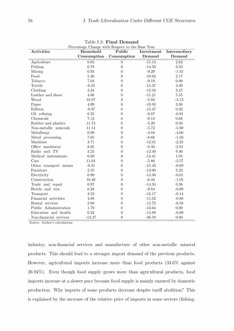
58 I. Trade Liberalisation Under Different CGE Structures

Table I.3: Final DemandPercentage Change with Respect to the Base Year

Activities Household Public Investment IntermediaryConsumption Consumption Demand Demand

Agriculture 0.05 0 -15.13 2.62Fishing 0.78 0 -14.50 3.33Mining 6.93 0 -9.29 -1.55Food 5.36 0 -10.62 2.17Tobacco 7.04 0 -9.19 0.00Textile -0.25 0 -15.37 3.39Clothing 3.34 0 -12.33 3.47Leather and shoes 4.66 0 -11.21 5.55Wood 10.87 0 -5.94 -3.13Paper 4.99 0 -10.93 3.38Edition -0.37 0 -15.47 0.32Oil refining 6.25 0 -9.87 -0.91Chemicals 7.12 0 -9.13 0.68Rubber and plastics 11.74 0 -5.20 0.50Non-metallic minerals 11.14 0 -5.72 -5.90Metallurgy 0.00 0 -4.84 -4.00Metal processing 7.65 0 -8.68 -1.50Machines 3.71 0 -12.01 -2.25Office machinery 8.05 0 -8.33 -2.91Radio and TV 3.25 0 -12.40 9.36Medical instruments 0.89 0 -14.41 1.05Cars 11.04 0 -5.80 -2.57Other transport means -0.31 0 -15.43 -0.69Furniture 2.55 0 -13.00 2.23Electricity 0.90 0 -14.40 -0.01Construction 10.40 0 -6.34 -1.05Trade and repair 0.97 0 -14.34 0.38Hotels and rest. 6.28 0 -9.84 -0.69Transport 3.53 0 -12.17 -0.14Financial activities 4.88 0 -11.02 -0.80Rental services 2.88 0 -12.72 -0.58Public Administration 1.79 0 -13.64 0.00Education and health 0.32 0 -14.89 -0.09Non-financial services -13.47 0 -26.59 0.80

Source: Author’s calculations.

industry, non-financial services and manufacture of other non-metallic mineral

products. This should lead to a stronger import demand of the previous products.

However, agricultural imports increase more than food products (33.6% against

26.94%). Even though food supply grows more than agricultural products, food

imports increase at a slower pace because food supply is mainly ensured by domestic

production. Why imports of some products decrease despite tariff abolition? This

is explained by the increase of the relative price of imports in some sectors (fishing,

59

clothing, oil refining, metallurgy, metal processing, office machinery, radio and

television, other transport means, hotels and restaurants, transport, financial and

rental services). Export increase replaces the drop of domestic production in some

sectors (mining, tobacco and wood industries, rubber and plastics, metallurgy,

metal processing, office machinery, car industry, other transport means, hotels

and restaurants, transport, rental and financial services). This transformation of

domestic sales into exports (Table I.2) is explained by lower domestic prices received

by local producers and is motivated by the real exchange rate depreciation as well

as lower imported input prices. Indeed, the domestic price declines with respect

to the price received by producers for their sales abroad, that is kept constant2.

Exports of other non-metallic mineral products and machines fell by 0.77% and

5.90% respectively, despite the drop of domestic prices by 11.11% and 6.32%. This

is explained by the fact that producers adjust their production downward following

the drop of internal demand. Exports of non-financial services decrease by 3.63%

because the domestic price increases by 13.18%. Producers are thus motivated by

higher domestic prices and offer their services on the domestic market.

With falling internal demand addressed to some sectors, producers reduce

their production (tobacco and wood industries, oil refining, rubber and plastics,

non metallic minerals, metallurgy, metal processing, machines, office machinery,

cars, construction services, hotels and restaurants, transport, financial and rental

services, public administration). The Leontief production function ensures a

perfect complementarity between value added and intermediary consumption so that

production adjustments are made possible by equal variations of value added and

intermediary consumption. It will shown in the next section how the specification

of the production function affects the results of trade liberalisation. All contracted

2 This stems from the fact that Morocco is a small open economy that does not affect internationalprices.

60 I. Trade Liberalisation Under Different CGE Structures

sectors reduce their demand for labour (Table I.4), the capital being sector-specific3.

Expanding sectors absorb the volume of labour released. Labour demand increases

the most in medical instruments and editing sectors (by 34.20% and 27.56%

respectively) because they display the highest production growth (14.21% and

12.98% respectively). Furthermore, labour demand grows strongly in non-financial

services, by 33.81%, while production only rises by 9.01%. This is explained by the

fact that non-financial services are more labour intensive than editing.

The increased demand for labour by the expanding sectors exceeds the amount of

labour released by the contracted ones. Given that total labour supply is fixed, the

wage must adjust upward in order to rebalance the market. However, the wage rate

decreases by about 4%. Indeed, the wage rate in the perfect competition market is

given by the product of the physical marginal productivity of labour and the value

added price. In the present case, it is the drop in the average value added price

that explains the declining wage. Since capital is sector-specific, the rental rate of

capital rises in sectors that ask for more labour, due to higher physical marginal

productivity of capital, and vice versa. Labour demand mostly increases in medical

instrument manufacturing and non-financial services, inducing the greatest increase

in the rental rate of capital (by 29.12% and 28.75% respectively). The greater decline

in labour demand occurs in non-metallic mineral products and machines (-18.25%

and -17.07% respectively) inducing the largest decline of capital return (-21.34%

and -20.21% respectively). However, in other transport means, electricity, trade and

repair, the rental rate of capital decreases (-3.39%, -1.27% and -2.23% respectively),

despite higher labour demand, due to lower value added prices.

In the sector “public administration and social security”, the value added is equal

to the wage payroll. Therefore, the production drop by 1.28%, following lower

3 In tradable sectors, firms maximise their profits. Then, if the capital available is sector-specific,the profit or capital remuneration is residual and varies from a sector to another. This approachis irrelevant for the public sector since the government, as a supplier of non-tradable services,does not have an optimising behaviour. The cost and thus the price of public services is theresult of the combination of wage and capital costs. Consequently, the rental rate of capital inthe public sector is normalised and capital demand is calculated residually (See Equation A8,Appendix C).

61

internal demand, leads to an equal decrease of the value added and labour demand.

By contrast, the production of public sector “education and health” increases by

0.26% due to higher internal demand, causing an equal increase of the value added

and the demand for production factors.

Table I.4: Value AddedPercentage Change with Respect to the Base Year

Activities Value Value Added Labour Capital CapitalAdded Price Demand Demand Return

Agriculture 0.13 0.76 4.86 0 0.89Fishing 1.44 -1.22 4.15 0 0.21Mining 1.88 -0.93 4.90 0 0.93Food 3.90 1.94 10.08 0 5.92Tobacco -1.17 -11.71 -9.31 0 -12.74Textile 2.40 -0.58 5.81 0 1.81Clothing 3.84 1.20 9.22 0 5.08Leather and shoes 5.94 1.08 11.29 0 7.08Wood -2.04 -11.43 -9.82 0 -13.23Paper 4.70 6.01 15.35 0 10.99Edition 12.98 8.63 27.56 0 22.73Oil refining -1.68 -11.25 -9.31 0 -12.74Chemicals 1.84 0.16 6.02 0 2.01Rubber and plastics -3.20 -5.12 -4.54 0 -8.15Non-metallic minerals -6.17 -16.17 -18.25 0 -21.34Metallurgy -2.71 -16.07 -15.14 0 -18.35Metal processing -3.59 -7.46 -7.28 0 -10.79Machines -8.84 -12.48 -17.07 0 -20.21Office machinery -3.15 -6.19 -5.58 0 -9.15Radio and TV 10.98 3.33 19.19 0 14.68Medical instruments 14.21 13.06 34.20 0 29.12Cars -3.84 -5.05 -5.11 0 -8.70Other transport means 0.18 -3.56 0.41 0 -3.39Furniture 2.06 -0.09 5.98 0 1.97Electricity 0.66 -1.91 2.62 0 -1.27Construction -6.27 -14.24 -16.46 0 -19.62Trade and repair 0.29 -2.51 1.62 0 -2.23Hotels and rest. -2.98 -12.72 -12.00 0 -15.33Transport -1.33 -6.04 -3.64 0 -7.28Financial activities -0.91 -8.64 -5.90 0 -9.47Rental services -0.20 -5.89 -2.38 0 -6.07Public Administration -1.28 -3.78 -1.28 0 0.00Education and health 0.26 -2.95 0.26 0.26 0.00Non-financial services 9.01 18.11 33.81 0 28.75Source: Author’s calculations.

Following the wage drop, household income decreases by 3%, firms’ income

by 2%, and government income by 20%. Given that the direct tax rate is

constant, household disposable income falls by 3% and so do households’ savings, the

62 I. Trade Liberalisation Under Different CGE Structures

propensity to save being constant. Firms’ savings also decrease (by 2.7%). Lower

households and firms’ income induces a fall in the amount of direct taxes collected

by the government and also helps explain the drop of government income.

In sum, trade liberalisation results in lower incomes for all economic agents.

However, this is not a handicap for household consumption since decreasing income

is accompanied by lower composite prices. The price effect is higher than the income

effect: the drop of the consumer price index more than compensates the drop of

income, so that household real income increases. Similarly, household welfare given

by the equivalent variation4 increases by MAD 3.9 billion, or by 1.3% of household

disposable income. Trade liberalisation has the strongest impact on public savings

and economic growth. It turns public current surplus (about +3% of GDP) to

a deficit (-2% of GDP) and reduces real GNP by 4.43%5. Moreover, when one

disaggregates the absolute change of real GNP, it appears that this negative evolution

is mainly driven by the contraction of the overall activity: real GDP drop explains

93% of GNP variation, it decreases by 4.11%. Medical instrument manufacturing

benefits the most from tariff removal, with a 14.21% rise in production. This

sector is one of the least protected ones, with an initial import tariff rate of 3.3%.

Therefore, trade liberalisation is likely to channel inputs from the most protected

sectors (rubber industry and other non-metallic minerals) to the least protected

ones (fishing, textile and clothing, leather industry, edition, radio and TV, medical

instruments, other transport means and non-financial services). All those sectors

expand. Although the food industry was the most protected sector, with an initial

tariff of 46.91%, it also expands after trade liberalisation by 3.9%. Note that

4 The equivalent variation is the measure of how much more money a consumer would need beforea price decrease, to be just as well off after the price decrease. It is given by Equation A45 inAppendix C).

5 Real GNP is calculated as follows:Real GDP at constant prices+ Commercial surplus or deficit resulting from the change in terms of trade= Real gross domestic income+ Real primary income received from the RoW- Real primary income sent to the RoW= Real gross national income= Real GNP.

63

the survival of this industry in spite of foreign competition is possible thanks to

government subsidies to food consumption. The subsidy rate is about 3%, further

reducing the composite price of food and maintaining domestic demand. In addition,

food producers benefit from an advantageous relative export price that stimulates

sales on international markets (6.04%). By contrast, the production of some sectors

decreases in spite of being among the least protected ones (oil refining, machines,

hotels and restaurants, transport, financial and rental services), affected by lower

internal demand.

2 Sensitivity Analysis

This section deals with the sensitivity of trade liberalisation results to the specific

assumptions of the EXTER model. EXTER is modified according to three standard

CGE models: GTAP (Brockmeier, 2001), IFPRI (Lofgren et al., 2002) and MIRAGE

(Bchir et al., 2002). The main differences between the three models allow to

investigate nine scenarios summarised in Table I.5. For each scenario, I present

a detailed discussion on how the results of trade liberalisation change with respect

to the original model structure.

Table I.5: Alternative ScenariosItem Scenario DefinitionSIM1 Production FunctionSIM2 Intermediate Consumption FunctionSIM3 Value Added FunctionSIM4 Investment Volume FunctionSIM5 Household Consumption FunctionSIM6 Investment-driven vs. Savings-drivenSIM7 The NumeraireSIM8 Imperfect vs. Perfect CompetitionSIM9 Time Dimension

64 I. Trade Liberalisation Under Different CGE Structures

2.1 Functional Forms

2.1.1 CES vs. Leontief

SIM1: Production Function

The degree of substitution between intermediary consumption and production

factors is inherently weak due to technical constraints. For this reason, EXTER

assumes perfect complementarity between intermediate consumption and value

added, by the means of a Leontief production function: changes in production

XS leads to the same percentage change in value added V A and intermediary

consumption CI. By contrast, GTAP and IFPRI assume a CES combination of

value added and intermediary consumption in the production function6. Now, there

is no reason for changes in the value added and intermediate consumption to be

equal to changes in production. It all depends on the variation of the value added

price PV relatively to the intermediate consumption price PIC, and the elasticity

of substitution 0 ≤ σps ≤ ∞ between these two components:

σ =d(CI/V A)

CI/V A/d(PV/PIC)

PV/PIC

If σps → 0, substitutability is impossible between value added and intermediary

consumption. If σps → ∞, value added and intermediary consumption are perfect

substitutes. The production function of private sector ps in EXTER must be

replaced by the following one:

XSps = Aps[αpsV A(σps−1)/σpsps + (1− αps)CI(σps−1)/σps

ps ]σps/(σps−1)

and intermediary consumption demand by:

CIps/V Aps = (1− αpsαps

PVpsPICps

)σps

6 In MIRAGE, the production function is a also a Leontief combination of value added andintermediate consumption.

65

where Aps is a scale parameter in the CES production function and αps a share

parameter in this function. An equation for the price of intermediate consumption

needs to be added to the model. The price of intermediary consumption by sector

is a weighted average of input composite prices PCi, the weights being the share of

each input in total intermediary consumption of the corresponding sector aijij:

PICj =∑i

PCiaijij

This new specification only applies to the private sector. The production function

in the public sector is still a Leontief: if the number of ministers increases, the

government must provide additional cars.

Different values are given to the elasticity of substitution according to sectors.

For example, in industry, a strong substitution between production factors and

intermediate inputs is barely tolerated. For this reason, I choose an elasticity

of substitution of 0.4 in industrial sectors. This relative complementarity is less

true in agriculture where the elasticity is fixed to 0.7. In services, the elasticity

of substitution is fixed to 1.1. At present, increasing production does not induce

an equal rise of value added and intermediate consumption, independently from

price changes. For the same increase in value added relative price, intermediary

consumption of tradable services rises the most, due to the highest elasticity of

substitution, followed by agriculture and industrial sectors.

Table I.6 shows that the intermediate consumption price of construction services

mostly decreases (10.41%) because 50% of contruction intermediate consumption

consist of non-metallic mineral and metal products, whose composite price decreases

by 12% and 13% respectively. However, the sharp decrease of value added price more

than compensates the drop of intermediary consumption price, so that intermediary

consumption falls. Therefore, when production decreases with respect to the

benchmark simulation, the value added decreases less (-5.18% instead of -6.27%)

and intermediate consumption decreases more (-7.65% instead of -6.27%). The

66 I. Trade Liberalisation Under Different CGE Structures

highest increase in the relative price of value added is recorded in non-financial

services (19.47%). Consequently, relative intermediate consumption mostly grows

in non-financial services (21.62%). Surprisingly, intermediary consumption in the

trade sector grows more than in medical instrument sector, despite a lower increase

in the relative price of value added. This is explained by the higher elasticity of

substitution in the service sector (1.1) compared to industry (0.4).

Table I.6: SIM1: The CES Production Function, Some Selected ResultsPercentage Change with Respect to the Base Year

Private Sectors PV PCI PV/PCI CI/VAAgriculture -0.03 -4.72 4.91 3.42Fishing -1.96 -5.29 3.52 2.45Mining -1.08 -6.96 6.31 2.48Food 0 -5.27 5.55 2.19Tobacco -10.08 -3.68 -6.64 -2.71Textile -0.4 -4.35 4.14 1.63Clothing 0.75 -3.46 4.36 1.72Leather and shoes 0.06 -6.6 7.14 2.79Wood -10.92 -8.77 -2.36 -0.95Paper 3.87 -7.33 12.08 4.67Edition 5.9 -6.79 13.62 5.23Oil refining -7.62 -7.3 -0.34 -0.14Chemicals -0.39 -7.51 7.7 3.01Rubber and plastics -4.59 -7.49 3.13 1.23Non-metallic minerals -14.76 -6.98 -8.37 -3.43Metallurgy -12.86 -8.34 -4.93 -2.01Metal processing -7.74 -9.03 1.41 0.56Machines -10.58 -4.98 -5.89 -2.4Office machinery -6.58 -8.79 2.42 0.96Radio and TV 2.43 -5.48 8.37 3.27Medical instruments 9.79 -4.54 15.01 5.72Cars -5.35 -9.02 4.03 1.59Other transport means -3.74 -4.8 1.11 0.45Furniture -1.47 -5.41 4.16 1.65Electricity -2.72 -7.4 5.04 5.57Construction -12.53 -10.41 -2.36 -2.6Trade and repair -2.41 -7.65 5.67 6.25Hotels and rest. -9.95 -6.88 -3.29 -3.61Transport -5.79 -5.92 0.13 0.15Financial activities -5.9 -5.92 0.02 0.02Rental services -4.75 -5.65 0.95 1.05Non-financial services 13.77 -4.77 19.47 21.62Source: Author’s calculations.

Table I.7 compares the main results of SIM1 to the benchmark simulation.

Production, value added and intermediary consumption change in the same direction

as before. However, the magnitude of the change is different now because, as

67

pointed out earlier, value added and intermediary consumption are affected by

the relative price change and the elasticity of substitution. In this context, the

only exceptions are rental services whose intermediary consumption increases now

by 0.96%, while it decreases at the benchmark simulation by the same amount

of production and value added (-0.2%). Indeed, production decreases less than

before (-0.01% instead of -0.2%) due to higher internal demand, and consequently,

value added and intermediate consumption increase with respect to the EXTER

simulation. The rising relative value added price results in a higher intermediate

consumption level. This price effect, combined to a lesser drop of production,

explains the increase of intermediate consumption by 0.96%.

When intermediary consumption varies with respect to the EXTER simulation,

input demand is affected as well as internal demand addressed to sectors. The effect

of intermediary consumption change on input demand is not reported here for the

sake of brevity, but still some points need to be clarified. To begin with, oil refining

products constitute 15% of intermediate consumption of the transport sector, 22%

of intermediate consumption of the electricity sector and 13% of intermediate

consumption of the fishing sector. The higher relative price of value added in

these sectors induces greater intermediary consumption, and consequently increased

consumption of all intermediate inputs, particularly oil refining products. This is

why the demand for oil refining inputs increases by 0.56% now while it previously

decreased by 0.91%. In the same way, it is possible to explain why total intermediary

demand of inputs from the electricity and transport sectors, financial activities,

construction, hotels and restaurants now rises, in contrast to the EXTER simulation.

Increasing internal demand addressed to some sectors can also boost imports

as well as internal production and have indirect effects on other variables in the

model. This is case for example of paper industry. Rising internal demand of paper

products stimulates imports and production for the local market (+17% instead

of +15% for imports and +7% instead of +5% for domestic production). Higher

imports and domestic production explain why indirect taxes increase now by 0.61%

68 I. Trade Liberalisation Under Different CGE Structures

while they were decreasing by 0.67% before. Rising demand for mining products

also explains the higher volume of imports (+3% against +2%) and production for

the local market (+1% against a 0.2% drop previously).

Finally, it is worth mentioning that the CES production function is hardly used

in the short run. A production function putty-clay7 would be better suited. The

new specification of the production function does not alter, once again, winners

and losers from trade liberalisation. Only the magnitude of variable changes is

modified: for example, the medical instrument sector expands more (+17.01%

instead of +14.21%). The greater expansion of production is made possible by

higher intermediate consumption, in comparison with the benchmark simulation,

due to the fall in the relative price of intermediary consumption. The classification

of winners and losers is also affected, albeit marginally. For example, non-metallic

mineral industry is henceforth the second loser, replacing the construction sector

that is now ranked third. Moreover, household welfare increases compared to the

benchmark simulation (by 1.7% against 1.3% of his disposable income) and the

economic contraction is slightly reduced (-4.02% instead of 4.11%).

SIM2: Intermediate Consumption Function

In the static EXTER model, intermediary consumption CI by sector ps is a Leontief

combination of intermediate inputs. Such formulation reflects the rigidity of the

production function in the short run: changes in input relative price is unlikely to

affect the structure of sectoral intermediary consumption. However, in the medium

and long run, as it is the case in the dynamic model MIRAGE, changes in input

relative price is able to affect, to some extent, the choice of intermediate goods. A

CES function is adopted in order to reflect the imperfect substitutability between

7 A putty-clay technology distinguishes between ex ante (or “putty”) and ex post (or “clay”)technology. Ex ante production technology will tend to have high substitution possibilities, andthus is probably closer to the smooth production functions of conventional Neoclassical models.However, ex post production technology has far fewer substitution possibilities, and thus is closerto the Leontief case.

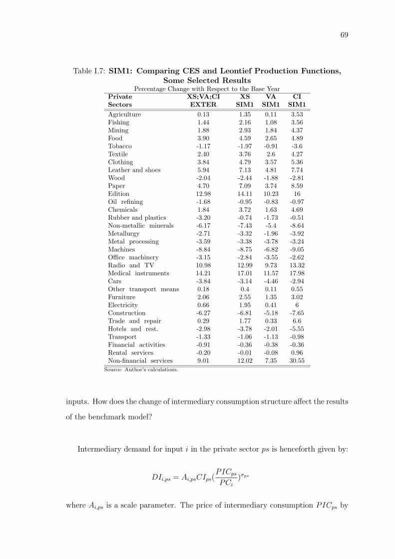
69

Table I.7: SIM1: Comparing CES and Leontief Production Functions,Some Selected Results

Percentage Change with Respect to the Base YearPrivate XS;VA;CI XS VA CISectors EXTER SIM1 SIM1 SIM1Agriculture 0.13 1.35 0.11 3.53Fishing 1.44 2.16 1.08 3.56Mining 1.88 2.93 1.84 4.37Food 3.90 4.59 2.65 4.89Tobacco -1.17 -1.97 -0.91 -3.6Textile 2.40 3.76 2.6 4.27Clothing 3.84 4.79 3.57 5.36Leather and shoes 5.94 7.13 4.81 7.74Wood -2.04 -2.44 -1.88 -2.81Paper 4.70 7.09 3.74 8.59Edition 12.98 14.11 10.23 16Oil refining -1.68 -0.95 -0.83 -0.97Chemicals 1.84 3.72 1.63 4.69Rubber and plastics -3.20 -0.74 -1.73 -0.51Non-metallic minerals -6.17 -7.43 -5.4 -8.64Metallurgy -2.71 -3.32 -1.96 -3.92Metal processing -3.59 -3.38 -3.78 -3.24Machines -8.84 -8.75 -6.82 -9.05Office machinery -3.15 -2.84 -3.55 -2.62Radio and TV 10.98 12.99 9.73 13.32Medical instruments 14.21 17.01 11.57 17.98Cars -3.84 -3.14 -4.46 -2.94Other transport means 0.18 0.4 0.11 0.55Furniture 2.06 2.55 1.35 3.02Electricity 0.66 1.95 0.41 6Construction -6.27 -6.81 -5.18 -7.65Trade and repair 0.29 1.77 0.33 6.6Hotels and rest. -2.98 -3.78 -2.01 -5.55Transport -1.33 -1.06 -1.13 -0.98Financial activities -0.91 -0.36 -0.38 -0.36Rental services -0.20 -0.01 -0.08 0.96Non-financial services 9.01 12.02 7.35 30.55

Source: Author’s calculations.

inputs. How does the change of intermediary consumption structure affect the results

of the benchmark model?

Intermediary demand for input i in the private sector ps is henceforth given by:

DIi,ps = Ai,psCIps(PICpsPCi

)σps

where Ai,ps is a scale parameter. The price of intermediary consumption PICps by

70 I. Trade Liberalisation Under Different CGE Structures

private sector ps is a weighted average of input composite prices PCi, the weights

being the share of each input in total intermediary consumption of the corresponding

sector aiji,ps:

PICps =∑i

PCiaiji,ps

The elasticity of substitution 0 ≤ σps ≤ ∞ between inputs 1 and 2 measures the

relative variation of input use following an infinitesimal variation of their relative

price.

σps =d(DI1,ps/DI2,ps)

DI1,ps/DI2,ps

/d(PC2/PC1)

PC2/PC1

In this exercise, σps is chosen equal to 0.5 in order to reflect the relative rigidity of

intermediate consumption in the short run.

In EXTER, intermediary consumption change induces an equal variation of all

input demand, regardless of the input relative prices. By contrast, input demand

is here affected by the price of composite products, according to an elasticity of

substitution equal to 0.5. For instance, the agricultural sector reduces the demand

of agricultural and textile inputs as well as electricity, water and education services to

the benefit of food and oil refining inputs, chemicals, rubber and plastics, machines,

construction, trade, transport and financial services, whose composite price sharply

falls following trade liberalisation8. Intermediate demand by the fishing sector for

agricultural and textile goods as well as transport means and non-financial services

also decreases to the benefit of inputs whose composite price sharply falls, such

as fishery and food products, mining and paper products, oil refining, chemicals,

rubber and plastics, metallurgy, metal processing, machines and equipment, office

machinery, radio and TV, furniture, electricity and water, trade services, hotels and

8 For the sake of brevity, the results are not reported here. However, they are available to theinterested reader at request.

71

restaurants, transport, construction and financial services. Intermediate demand for

the above-mentioned less demanded inputs was rising in the benchmark simulation.

Moreover, intermediate demand of wood, rubber and non-metallic minerals increases

in the majority of sectors because their composite price sharply falls.

Sectoral intermediary consumption, by modifying the demand for inputs orig-

inated from different sectors, affects internal demand addressed to sectors and

consequently sectoral production. This is the case for example of total intermediate

demand of trade services that decreases now, by contrast to the benchmark simu-

lation, inducing a reduction of total domestic demand for these goods. Producers

then adjust downward their production (by 0.01% instead of a positive evolution of

0.29% previously).

The change of intermediary consumption structure affects the results of trade

liberalisation: trade services add to losers. Indeed, the Leontief function is somewhat

extreme, in the sense that intermediate demand for inputs is independent on changes

in relative prices. But trade liberalisation primarily affects prices. Therefore, it is

likely to modify the demand for inputs as well as total demand addressed to sectors

and thus production level. In addition, sectoral classification changes following tariff

removal. For example, radio and TV industry replaces the editing sector as the

second winner (Table I.8).

The elasticity of substitution seems to play an important role because it

determines the intensity of input demand variation following the change in input

relative prices. For this reason, two additional simulations, SIM2B and SIM2C,

are also run, one with an elasticity of 0.8 and the other with an elasticity of

1.1. When the elasticity is equal to 0.8, rubber industry adds to winners: rubber

production increases by 1.12% after being decreasing by 3.20% in the EXTER

simulation. When it is equal to 1.1, rubber industry adds again to winners, and

other transport means to losers. The production of the latter falls by 0.08%

72 I. Trade Liberalisation Under Different CGE Structures

after being increasing by 0.18% in the benchmark simulation9. Indeed, the higher

the elasticity of substitution between inputs is, the more input demand reacts to

changes in relative prices following trade liberalisation, and the more total internal

demand addressed to sectors varies. Given that other things ar equal, producers

then adjust their production in order to meet domestic demand. Consequently, the

sectoral classification of losers and winners changes with respect to the benchmark

simulation. Finally, it is worth mentioning that the change of intermediary

consumption structure leads to a slight welfare improvement. Welfare also increases

with the elasticity of substitution (1.4%, 1.5% and 1.6% of household disposable

income respectively instead of 1.3% in the EXTER simulation). In addition, the

economic contraction slightly decreases (-4.10% for the 3 simulations instead of -

4.11%).

2.1.2 CES vs. Cobb-Douglas

SIM3: Value Added Function

GTAP, IFPRI and MIRAGE suppose an imperfect substitutability between factors

in the value added, by the means of a CES function. The latter allows richer

behaviours than the Cobb-Douglas function of EXTER. The adoption of this

functional form is justified in MIRAGE by the need to illustrate the relative

complementarity between skilled labour and capital, highlighted in empirical studies.

Value Added is thus a CES function of land, natural resources, unskilled labour and

a composite factor of skilled labour and capital, the last term being itself a CES

function of its components. The elasticity of substitution within the capital and

skilled labour bundle is assumed to be 0.6 while the elasticity between this bundle

and all other factors is fixed to 1.1.

When the value added V A is a CES function of labour LD and capital KD, it

9 Recall that this sector is among the least protected ones. Therefore, the decrease of transportprice following tariff removal is weak in comparison to other commodities.

73

Table I.8: SIM2: The Effects on Productionof a Leontief and a CES Intermediary Consumption Function

Percentage Change with Respect to the Base YearPrivate Sectors EXTER SIM2A SIM2B SIM2CAgriculture 0.13 0.12 0.11 0.1Fishing 1.44 1.37 1.29 1.2Mining 1.88 2.3 2.46 2.58Food 3.90 4.49 4.79 5.07Tobacco -1.17 -1.15 -1.15 -1.15Textile 2.40 2.15 1.94 1.72Clothing 3.84 4.12 4.24 4.34Leather and shoes 5.94 6.43 6.58 6.69Wood -2.04 -1.55 -1.33 -1.14Paper 4.70 5.14 5.28 5.37Edition 12.98 12.64 12.43 12.22Oil refining -1.68 -1.34 -1.2 -1.08Chemicals 1.84 2.44 2.69 2.9Rubber and plastics -3.20 -0.45 1.12 2.66Non-metallic minerals -6.17 -5.44 -5.06 -4.73Metallurgy -2.71 -1.66 -1.2 -0.83Metal processing -3.59 -3.25 -3.09 -2.95Machines -8.84 -8.62 -8.59 -8.58Office machinery -3.15 -2.93 -2.81 -2.7Radio and TV 10.98 12.76 13.28 13.63Medical instruments 14.21 15.46 15.8 16.01Cars -3.84 -3.1 -2.7 -2.32Other transport means 0.18 0.15 0.05 -0.08Furniture 2.06 2.28 2.34 2.37Electricity 0.66 0.37 0.23 0.11Construction -6.27 -6.57 -6.72 -6.86Trade and repair 0.29 -0.01 -0.11 -0.19Hotels and rest. -2.98 -3.02 -3.03 -3.04Transport -1.33 -1.39 -1.44 -1.49Financial activities -0.91 -0.83 -0.81 -0.79Rental services -0.20 -0.25 -0.27 -0.29Non-financial services 9.01 8.49 8.21 7.97

Notes: (1) SIM2A: σps = 0.5(2) SIM2B: σps = 0.8(3) SIM2C: σps = 1.1Source: Author’s calculations.

has the following form:

V Aps = Aps[αpsLD(σps−1)/σpsps + (1− αps)KD(σps−1)/σps

ps ]σps/(σps−1)

and labour demand is then given by:

LDps/KDps = (αps

1− αpsrpsw

)σps

74 I. Trade Liberalisation Under Different CGE Structures

where 0 ≤ σps ≤ ∞ is the constant elasticity of substitution between labour and

capital, Aps a scale parameter in the CES function and αps a share parameter in

this function. If σps → 0, substitutability is impossible and inputs are perfect

complements. If σps → ∞, inputs are perfect substitutes. σ measures the relative

variation of factor use following an infinitesimal variation of their relative price.

σ =d(KD/LD)

KD/LD/d(w/r)

w/r

The degree of substitution between production factors differs according to sectors.

For example, in industry, a strong substitution between labour and capital is barely

tolerated: some technologies can hardly be substituted by labour. For this reason, I

choose an elasticity of substitution of 0.4 in industrial sectors, reflecting the relative

complementarity between labour and capital. This relative complementarity is less

true in agriculture where the elasticity is fixed to 0.7. In services, some activities

such as “hotels and restaurants”, tolerate a strong elasticity of substitution between

labour and capital. Indeed, if the wage strongly increases, it is possible to replace

workers that wash dishes by machines. In this case, the elasticity of substitution

is fixed to 1.1. The perfect complementarity is kept between labour and capital in

non-tradable services, as it was the case in EXTER adapted to the Moroccan SAM.

The unitary elasticity of substitution between labour and capital in the Cobb-

Douglas function implies that the change in the relative price of labour and capital

induces an equal change of the relative demand for these two inputs. When the

elasticity of substitution falls below 1, like in industrial and agricultural sectors,

relative factor demand reacts less to the variation of their relative price. For tradable

services, an elasticity of substitution greater than 1 implies a stronger reaction of

relative factor demand to the change of their relative price. In what follows, the

analysis is made with respect to the benchmark simulation.

For the same variation of relative factor price and given that other things are

equal, labour demand must decrease with respect to the benchmark simulation in

75

agricultural and industrial sectors and increase in tradable services. Table I.9 shows

that labour demand in agricultural and industrial sectors moves in the same direction

as in the benchmark simulation, increasing or decreasing but always less than before.

This is also explained by the drop of the production with respect to the EXTER

simulation. Only labour demand increases in “other transport means”, with respect

to the benchmark simulation, because at the present case, this sector expands with

respect to the EXTER simulation. In tradable services, labour demand grows more

in the electricity sector and non-financial services, reflecting the strong elasticity of

substitution (1.1). However, in the remaining tradable services, it decreases less,

because production increases with respect to the benchmark simulation. In “trade

and repair”, labour demand decreases when compared to EXTER, following lower

production growth. Lower labour demand in agricultural and industrial sectors

reduces the wage rate with respect to the benchmark simulation (-5.13% against

-3.78%).

The adoption of a CES value added function also has indirect effects on the

remaining variables of the model. Here are some examples: first, the negative

evolution (-2.5%) of the editing composite price at the benchmark simulation turns

to be positive (+0.85%) now. Indeed, the lower reaction of labour demand to factor

relative price variation induces a lower growth of labour demand (19.89% against

27.56%), and ceteris paribus, a weaker increase of value added and production10

(8.85% against 12.98%). The lower rise of production results in weaker exports

(+8% instead of 14%) and lower volume of production intended for the local market

(9% against 13%). If the demand level is the same as in the EXTER simulation,

producers raise their price by 2.4% (it decreased before by 1.72%). Consequently,

the market price of domestic products also increases as well as the composite price.

The same logic applies for medical instruments to describe the weaker drop of the

composite price. Secondly, agricultural production intended for the local market

decreases by 0.08% now, instead of a positive change of 0.02% before. The weaker

10 Recall that production is a Leontief combination of value added and intermediary consumption.Therefore, value added, intermediary consumption and production vary in the same proportions.

76 I. Trade Liberalisation Under Different CGE Structures

reaction of labour demand to the wage relative variation induces, ceteris paribus a

weaker increase of agricultural value added and production. Thirdly, exports of non-

metallic minerals increase by 3.1% now whereas they fall by 0.77% in the benchmark

simulation. Indeed, the lower decrease of labour demand limits the production fall,

that in turn, makes possible export increase.

In sum, although the CES function allows richer behaviours than the Cobb-

Douglas, the results of the trade liberalisation shock on the Moroccan economy are

only marginally affected: the modifications are limited to the amplitude of variable

change, in particular the variation in labour demand, value-added and production.

The impact on welfare is weaker but still positive (about 1% instead of 1.3% of

household disposable income), and economic contraction is slightly reduced (-4.10%

rather than -4.11%). However, the classification of winners from trade liberalisation

is modified: non-financial services is henceforth ranked first instead of medical

instruments that is now classified after the editing sector.

SIM4: Investment Volume Function

In section 2, it was argued that trade liberalisation reduces government savings

and, given that other things are equal, total investment value. In turn, the drop of

total investment should lead, ceteris paribus, to a proportional fall in the demand

of each investment good:

INVi =µiIT

PCi

where INVi represents the investment demand of product i, PCi the composite price

of good i, µi the proportion of good i in total investment volume ITV OL, IT total

investment value given by: IT = ITV OL×PINV , and PINV the aggregate price

of investment. This reproduces the facts that total investment volume in EXTER

is a Cobb-Douglas function of investment products.

77

Table I.9: SIM3: Comparing CES and Cobb-Douglas Value AddedFunctions, Some Selected Results

Percentage Change with Respect to the Base YearPrivate Production / Labour Production / LabourSectors Value Added Demand Value Added Demand

EXTER EXTER SIM3 SIM3Agriculture 0.13 4.86 0.1 3.86Fishing 1.44 4.15 1.35 3.9Mining 1.88 4.90 1.46 3.86Food 3.90 10.08 3.04 8.09Tobacco -1.17 -9.31 -0.46 -3.68Textile 2.40 5.81 1.38 3.37Clothing 3.84 9.22 2.23 5.43Leather and shoes 5.94 11.29 4.3 8.36Wood -2.04 -9.82 -0.92 -4.42Paper 4.70 15.35 2.85 9.6Edition 12.98 27.56 8.85 19.89Oil refining -1.68 -9.31 -1.12 -6.05Chemicals 1.84 6.02 1.21 4Rubber and plastics -3.20 -4.54 -2.97 -4.18Non-metallic minerals -6.17 -18.25 -4.74 -13.32Metallurgy -2.71 -15.14 -1.17 -6.51Metal processing -3.59 -7.28 -2.57 -5.13Machines -8.84 -17.07 -7.25 -13.44Office machinery -3.15 -5.58 -1.71 -3.02Radio and TV 10.98 19.19 7.76 14.02Medical instruments 14.21 34.20 8.33 21.19Cars -3.84 -5.11 -2.97 -3.93Other transport means 0.18 0.41 0.65 1.49Furniture 2.06 5.98 1.54 4.53Electricity 0.66 2.62 0.77 3.06Construction -6.27 -16.46 -5.39 -14.31Trade and repair 0.29 1.62 0.21 1.2Hotels and rest. -2.98 -12.00 -2.96 -11.97Transport -1.33 -3.64 -0.99 -2.73Financial activities -0.91 -5.90 -0.85 -5.55Rental services -0.20 -2.38 -0.13 -1.59Non-financial services 9.01 33.81 9.51 35.53Source: Author’s calculations.

By contrast, MIRAGE assumes that total investment volume is a CES function

of investment demand by product. The constant elasticity of substitution is fixed

to 0.6 so that to reflect the relative rigidity of the production structure in the short

run: the change of investment product relative prices should not have a significant

effect on the demand of investment goods. Investment demand of product i is now

78 I. Trade Liberalisation Under Different CGE Structures

given by:

INVi = BiITV OL(PINV

PCi)σ

where Bi is a scale parameter and σ the elasticity of substitution between investment

products. σ was equal to unity in EXTER. The drop of the elasticity to 0.6

implies lower reaction of investment demand to relative price changes. PINV is

the investment aggregate price given by the following equation:

PINV × ITV OL =∑i

PCiINVi

How do the results of the benchmark simulation change following the CES

specification of the investment volume?

The drop of the investment aggregate price (-12%) should stimulate, ceteris

paribus, total investment volume and induce a proportional increase in investment

demand of all goods and services. Surprisingly, total investment volume decreases

by 6.5%, despite the drop of the aggregate investment price, because total savings

decrease by 18%, also reducing total investment value. Lower investment volume

causes a decline in investment demand of goods and services. My concern is how

investment demand by product changes with respect to the benchmark simulation.

It happens that investment demand for some products (fishing, tobacco, textile,

clothing, leather, oil refining, metal processing, machines, office machinery, radio

and TV, transport means, trade services, hotels and retsaurants, transport, financial

and rental services) increases with respect to the benchmark simulation, despite a

higher composite price (Table I.10). Indeed, at present, the reaction of investment

demand to the same change in prices is weaker than EXTER due to lower elasticity

of substitution between investment goods (0.6 rather than 1). Higher investment

demand with respect to the benchmark simulation stimulates, ceteris paribus,

internal demand addressed to sectors so that, as shown in Table I.11, firms adjust

79

their production upward in the above-mentioned sectors.

By contrast, investment demand of wood, rubber and plastics, non-metallic min-

erals and construction services decrease with respect to the benchmark simulation

despite a lower composite price. This is also explained by the weaker reaction of

investment demand to price changes. In addition, it happens that the share of

investment demand in total domestic demand addressed to these sectors is high.

Therefore, when total investment volume decreases, it induces a significant drop in

the demand addressed to them. The depressive effect on domestic demand is greater

in wood industry and non-metallic minerals, inducing a stronger contraction of their

production activity.

The changes in results due the new functional form of investment volume are

not strong enough to reverse the sign of production variation. However, the ranking

of winners is somewhat modified: medical instrument manufacturing is always the

first winner, but is now followed by radio and TV industry instead of the editing

sector, which is henceforth ranked third. I also investigate the sensitivity of the

results to different choices of the constant elasticity of substitution. Two additional

simulations are run, one with an elasticity of 0.8 (SIM4B), the other with an elasticity

of 1.1 (SIM4C). The classification of winners and losers is only marginally altered

and no changes in signs with respect to SIM4A are detected. Finally, in the three

simulations, household welfare improves (by 1.6% of household disposable income

instead of 1.3%) and the economic contraction is slightly attenuated for SIM4A and

SIM4B (-4.08% and -4.10% instead of -4.11%) and emphasised for SIM4B (-4.13%

instead of -4.11%).

2.1.3 LES vs. Cobb-Douglas

SIM5: Household Consumption Function

In EXTER, household utility is a Cobb-Douglas function of saving propensity and

commodity consumption. The Cobb-Douglas choice is not without consequences on

80 I. Trade Liberalisation Under Different CGE Structures

Table I.10: SIM4: Comparing CES and Cobb-Douglas InvestmentVolume Functions, Some Selected Results

Percentage Change with Respect to the Base YearActivities PC INV PC INV

EXTER EXTER SIM4A SIM4AAgriculture -2.9 -15.13 -3.47 -11.59Fishing -3.61 -14.5 -3.47 -11.59Mining -9.15 -9.29 -9.22 -8.27Food -7.8 -10.62 -8.07 -8.96Tobacco -9.24 -9.19 -8.99 -8.41Textile -2.62 -15.37 -2.56 -12.09Clothing -5.99 -12.33 -5.89 -10.24Leather and shoes -7.18 -11.21 -7.18 -9.49Wood -12.38 -5.94 -12.56 -6.19Paper -7.47 -10.93 -7.94 -9.04Edition -2.5 -15.47 -3.25 -11.71Oil refining -8.57 -9.87 -8.41 -8.76Chemicals -9.31 -9.13 -9.33 -8.21Rubber and plastics -13.06 -5.2 -13.09 -5.84Non-metallic minerals -12.59 -5.72 -12.72 -6.08Metallurgy -13.39 -4.84 -13.36 -5.67Metal processing -9.76 -8.68 -9.7 -7.98Machines -6.33 -12.01 -6.22 -10.04Office machinery -10.09 -8.33 -10.05 -7.76Radio and TV -5.92 -12.4 -5.77 -10.3Medical instruments -3.71 -14.41 -3.74 -11.44Cars -12.52 -5.8 -12.49 -6.23Other transport means -2.55 -15.43 -2.49 -12.12Furniture -5.27 -13 -5.3 -10.57Electricity -3.72 -14.4 -3.91 -11.35Construction -12.01 -6.34 -12.13 -6.46Trade and repair -3.79 -14.34 -3.55 -11.55Hotels and rest. -8.6 -9.84 -8.29 -8.83Transport -6.16 -12.17 -5.78 -10.29Financial activities -7.38 -11.02 -7.04 -9.57Rental services -5.57 -12.72 -5.28 -10.58Public administration -4.57 -13.64 -4.63 -10.95Education -3.17 -14.89 -3.27 -11.7Non-financial services 12.26 -26.59 5.61 -16.23Source: Author’s calculations.

elasticities: price elasticity, income elasticity and elasticity of substitution are all

equal to unity, and cross-price elasticity is zero. Such assumptions are quite strong

and unrealistic.

MIRAGE and IFPRI make use for household consumption of a functional form

somewhat more complicated than the Cobb-Douglas and CES functions: the linear

81

Table I.11: SIM4: The effects on Productionof a CES and a Cobb-Douglas Investment Volume Function

Percentage Change with Respect to the Base YearActivities EXTER SIM4A SIM4B SIM4CAgriculture 0.13 0.11 0.12 0.14Fishing 1.44 1.56 1.5 1.41Mining 1.88 1.86 1.88 1.88Food 3.9 3.89 3.89 3.91Tobacco -1.17 -1.08 -1.12 -1.2Textile 2.4 2.83 2.63 2.27Clothing 3.84 3.93 3.89 3.81Leather and shoes 5.94 5.92 5.93 5.94Wood -2.04 -2.13 -2.07 -2.04Paper 4.7 4.09 4.37 4.9Edition 12.98 10.59 11.7 13.7Oil refining -1.68 -1.45 -1.55 -1.76Chemicals 1.84 1.85 1.85 1.84Rubber and plastics -3.2 -3.2 -3.18 -3.22Non-metallic minerals -6.17 -6.26 -6.17 -6.2Metallurgy -2.71 -2.67 -2.67 -2.75Metal processing -3.59 -3.39 -3.46 -3.68Machines -8.84 -7.54 -8.16 -9.21Office machinery -3.15 -2.88 -2.98 -3.27Radio and TV 10.98 11.98 11.5 10.7Medical instruments 14.21 13.16 13.66 14.51Cars -3.84 -4.17 -3.97 -3.81Other transport means 0.18 0.72 0.46 0.04Furniture 2.06 1.91 1.98 2.12Electricity 0.66 0.63 0.64 0.66Construction -6.27 -6.39 -6.28 -6.31Trade and repair 0.29 0.38 0.34 0.26Hotels and rest. -2.98 -2.63 -2.79 -3.09Transport -1.33 -0.95 -1.14 -1.43Financial activities -0.91 -0.75 -0.82 -0.96Rental services -0.2 -0.15 -0.17 -0.21Public administration -1.28 -1.02 -1.15 -1.36Education 0.26 0.19 0.22 0.28Non-financial services 9.01 5.57 7.06 10.18

Notes: (1) SIM4A: σ = 0.6(2) SIM4B: σ = 0.8(3) SIM4C: σ = 1.1Source: Author’s calculations.

expenditure system (LES)11. This functional form allows a richer consumption

behaviour due to the existence of a minimum consumption level by commodity,

as well as non-unitary income elasticities. In other words, the budgetary shares of

commodities vary with changes in the consumption budget. Supernumerary income,

11 The LES demand function is obtained from a maximisation problem of the Stone-Geary utilityfunction (Stone, 1954).

82 I. Trade Liberalisation Under Different CGE Structures

i.e. the consumption budget minus the minimum consumption value of all products,

is divided among commodities according to a Cobb-Douglas function in IFPRI and

a CES function in MIRAGE. The representative household’s consumption of good i

is then given by12:

Ci = Cmini +γiPCi

(BC −∑i

PCiCmini) (I.1)

where BC represents household consumption budget, PCi the composite price of

good i, γi the budgetary share of good i in supernumerary income and Cmini the

minimum consumption volume of good i. Minimum consumption by commodity is

exogenous and the consumption budget is given by the following equation:

BC = Y DH − S“hh”

where Y DH represents household disposable income and S“hh” household savings.

With the LES, the calibration procedure is more complex and needs to be

clarified. First, income elasticities are adjusted in order to respect Engel aggregation:

the income elasticity-weighted sum of individual consumptions divided by total

consumption must equal one.

∑i εiPCiCiBC

= 1

with εi the income elasticity of demand of good i. Secondly, budgetary shares γi are

calibrated from adjusted income elasticities of demand:

εi =γiBC

PCiCi

Finally, the Frisch parameter, defined as the negative value of the ratio of household

12 This equation implies that the supernumerary income is a Cobb-Douglas function of consumptiongoods, as it is the case in IFPRI.

83

consumption budget to supernumerary income:

Frisch = − BC

BC −∑

i PCiCmini

is used to calibrate the minimum consumption volume by commodity Cmini from

equation (I.1).

Income elasticities were estimated by the Economic Research Service (ERS) of

the US Department of Agriculture (Bernstein et al., 2003) for the following groups:

beverages and tobacco, clothing and footwear, fuel and power, house operations,

medical care, education, transport and communication, recreation and others. For

food products, income elasticities were estimated for bread and cereals, meat, fish,

dairy products, fats and oils, fruits and vegetables, other food products. Data come

from the International Comparison Project Data (ICP) of the World Bank for the

year 1996.

If any changes in results may occur, they mainly concern consumption levels.

The increase of household consumption budget, as in the benchmark simulation,

should not lead, ceteris paribus, to a proportional increase in the consumption

of all commodities. Consumption volumes depend now on income elasticities,

besides changes in relative prices. Let me point out that lower prices reduce the

total value of minimum consumption and consequently, the supernumerary income

increases. Table I.12 shows that household consumption of almost all products

grows. Household demand mostly increases for commodities whose income elasticity

is the highest (such as wood, rubber, non-metallic minerals, cars and construction

services). For instance, consumption of transport services increases more than food

(+4.02% against +3.53%), despite the sharper drop of the food composite price (-

8.41% compared to -5.96% for transportation services). This is explained by Engel

law: income elasticity of food demand is positive but lower than 1. Indeed, the

estimated elasticity of food demand is equal to 0.69. The income elasticity of

84 I. Trade Liberalisation Under Different CGE Structures

transport demand is 1.22. Now, it becomes clear why the consumption of transport

services increases more.

It is easy to notice that consumption volumes change with respect to the

benchmark simulation where the income elasticity of demand was equal to unity.

For example, the consumption of mining products increases in comparison to the

EXTER simulation (+7.61% against +6.93% before) despite a lower drop of the

composite price. This is explained by the greater income elasticity of mining

products that is now equal to 1.36. The same reasoning applies to the following

sectors whose income elasticities are greater than 1: paper industry, edition,

chemicals, rubber industry, non-metallic minerals, metal processing, radio and TV,

medical equipment manufacturing, transport means, furniture industry, electricity

services, hotels and restaurants, transport, rental and financial services, public

administration, education and health. Furthermore, a reversal in consumption

change is detected for the consumption of editing and transport means. By contrast,

consumption of food decreases with respect to the benchmark simulation (positive

evolution of 3.53% rather than 5.36% before) despite a stronger drop of the composite

price. This is due to the fact that income elasticity of food demand is now lower

than 1. The same logic helps explain any decrease in the consumption of tobacco

and clothing.

A LES utility function affects the behaviour of household consumption, and

consequently the demand addressed to sectors as well as production level. Thus,

it is not surprising to see that the classification of winners and losers from trade

liberalisation is modified. However, no sign reversal in sectoral production growth

is detected. Household welfare improves by 1.4% of household disposable income

(instead of 1.3%) and economic contraction is slightly attenuated (-4.09% instead

of -4.11%). Finally, it is worth mentioning that the LES function is hardly used in

the case of poor countries where total minimum consumption value might exceed

household income.

85

Table I.12: SIM5: Comparing LES and Cobb-Douglas ConsumptionFunctions, Some Selected Results

Percentage Change with Respect to the Base YearActivities Prod. PC C Prod. PC C

EXTER EXTER EXTER SIM5 SIM5 SIM5Agriculture 0.13 -2.9 0.05 0.11 -3.35 0.66Fishing 1.44 -3.61 0.78 1.04 -3.95 1.49Mining 1.88 -9.15 6.93 1.8 -9.04 7.61Food 3.9 -7.8 5.36 2.19 -8.41 3.53Tobacco -1.17 -9.24 7.04 -1.33 -9.84 6.06Textile 2.4 -2.62 -0.25 2.27 -2.57 -0.85Clothing 3.84 -5.99 3.34 3.6 -5.99 3.04Leather and shoes 5.94 -7.18 4.66 5.4 -7.32 3.93Wood -2.04 -12.38 10.87 -2.14 -12.48 10.05Paper 4.7 -7.47 4.99 4.93 -7.24 5.76Edition 12.98 -2.5 -0.37 14.91 -1.89 0.65Oil refining -1.68 -8.57 6.25 -1.75 -8.58 6.32Chemicals 1.84 -9.31 7.12 1.9 -9.18 7.76Rubber and plastics -3.2 -13.06 11.74 -3.6 -13 11.97Non-metallic minerals -6.17 -12.59 11.14 -6.24 -12.5 11.39Metallurgy -2.71 -13.39 0 -2.78 -13.41 0Metal processing -3.59 -9.76 7.65 -3.7 -9.76 8.38Machines -8.84 -6.33 3.71 -8.74 -6.38 4.33Office machinery -3.15 -10.09 8.05 -3.22 -10.07 7.69Radio and TV 10.98 -5.92 3.25 11.09 -5.92 3.93Medical instruments 14.21 -3.71 0.89 15.15 -3.67 2.3Cars -3.84 -12.52 11.04 -3.99 -12.53 10.24Other transport means 0.18 -2.55 -0.31 0.53 -2.52 1.09Furniture 2.06 -5.27 2.55 2.59 -5.1 3.22Electricity 0.66 -3.72 0.9 0.86 -3.08 1.53Construction -6.27 -12.01 10.4 -6.33 -11.92 9.49Trade and repair 0.29 -3.79 0.97 0.15 -4.06 2.66Hotels and rest. -2.98 -8.6 6.28 -2.71 -8.27 7.52Transport -1.33 -6.16 3.53 -1.35 -5.96 4.02Financial activities -0.91 -7.38 4.88 -0.87 -6.97 5.48Rental services -0.2 -5.57 2.88 -0.17 -5.1 3.22Public administration -1.28 -4.57 1.79 -1.27 -4.37 2.94Education 0.26 -3.17 0.32 0.59 -3 1.31Non-financial services 9.01 12.26 -13.47 12.07 18.63 -14.68Source: Author’s calculations.

2.2 Macroeconomic Constraints

SIM6: Investment-driven vs. Savings-driven

EXTER has a savings-driven determination of investment: public expenditures

and tax rates are fixed. Government and firms’ savings are determined by the

model. Household savings are a fixed share of household disposable income. External

86 I. Trade Liberalisation Under Different CGE Structures

savings are fixed. Hence, none of the four types of savings is free to equilibrate the

aggregate savings-investment balance. Consequently, gross fixed capital formation

varies endogenously to achieve savings-investment equilibrium. However, in a static

model like EXTER, the most appropriate closure would be the one that considers

the volume of investment fixed. In a short term horizon, the rigidity of production

structure implies that investment demand is unlikely to change when shocks affect

aggregate savings.

In the IFPRI model, the savings-investment closure considers investment demand

by commodity fixed in volume. If it is so, and if savings are not flexible, there is

no guarantee for the savings-investment equilibrium to be achieved. Something

must be released in the savings side. In the IFPRI model, household savings are

released: instead of being a fixed share of disposable income, they adjust freely by

the means of a fully flexible adjustment term that is added to the saving propensity.

IFPRI macroeconomic closure is therefore “investment-driven”. Since the volume of

investment demand by product is now fixed, the equations that help determine this

variable are removed from the benchmark model.

At present, when tariff removal reduces government’s income and savings,

household savings must adjust upward in order to maintain the volume of investment

by product fixed. Household savings increase by 35.76% whereas it was decreasing

by 2.86% in the benchmark simulation (Table I.13). When household savings

increase, the share of disposable income spent on consumption should decrease,

ceteris paribus, as well as household consumption by product. However, this is not

always the case. Consumption of goods and services depends on changes in relative

prices.

Rubber products exhibit the largest reduction of their composite price (-13%).

That is why households mostly increase their consumption of rubber goods (6.12%).

In the benchmark simulation, the composite price of rubber products also decreased

by 13.06% but household consumption increased by 11.74% (Table I.14). The lower

consumption growth of rubber products with the new macroeconomic closure, for

87

Table I.13: SIM6: The Effect on Income of Investment and Savings-drivenClosures

Percentage Change with Respect to the Base YearHousehold Income Disposable Savings Consumption

Income BudgetEXTER -2.80 -2.86 -2.86 -2.86SIM6 -3.15 -3.21 35.76 -7.67Source: Author’s calculations.

the same drop of the composite price as before, is explained by the sharp drop of

household consumption budget (-7.67% instead of -2.86% before).

When the consumption budget decreases, households reduce their demand for

commodities whose relative price declines the least. Such is the case for example

of the following products: fishery, tobacco, clothing, leather, oil refining, machines,

radio and TV, medical instruments, furniture, electricity, trade and construction

services, hotels and restaurants, transport, rental and financial services, public

administration, health and education. By contrast to the EXTER simulation,

the consumption of those products decreases now. Only the consumption of non-

financial services increases with respect to the benchmark simulation (negative

change of 0.84% instead of 13.47% before) because the composite price declines

now by 6.88%, after being increasing by 12.26% in EXTER.

If lower consumption depresses the demand addressed to sectors in comparison

with the benchmark simulation, the stability of investment demand now compensates

for this loss. Recall that before, investment demand by product was decreasing.

Therefore, how internal demand changes with respect to the benchmark simulation

depends on the weight of household consumption and investment demand in total

demand. When consumption loss outweighs the positive effect of investment

stability, total internal demand decreases, and producers adjust their production

downward. This is the case of nearly half of the sectors (Table I.14). More interesting

is the fact that some of the expanding sectors in the benchmark simulation contract

now. Such is the case of agriculture, paper industry, edition, furniture industry,

electricity and education services, and non-financial services. Conversely, domestic

88 I. Trade Liberalisation Under Different CGE Structures

demand addressed to the other sectors increases and help explain production growth

with respect to the EXTER simulation. More specifically, oil refining and office

machinery sectors expand now, after being contracting in the benchmark simulation.

By contrast to the EXTER simulation, intermediate demand of mining products

increases by 0.13% (it fell by 1.55% before) because mining inputs constitute 62% of

total intermediary consumption of oil refining industry and 11% of total intermediary

consumption of non-metallic mineral products. At present, the production of oil

refining and non-metallic minerals increases with respect to the EXTER simulation

and so does the demand of inputs used intensively in these sectors, such as mining

products. The same logic helps explain the rising intermediate demand of oil refining

and metal processed products, office machinery, other transport means, electricity

services, hotels and restaurants, transport and construction services. Conversely,

intermediate demand of paper products decreases with respect to the EXTER

simulation (negative evolution of 0.01% rather than positive change of 3.38% before)

despite a lower composite price (negative change of 10.6% instead of 7.47%). This

is due to the fact that paper products constitute 54% of intermediary consumption

of paper industry and 57% of intermediary consumption of the editing sectors. The

contraction of paper and editing sectors explain the drop of paper input demand.

The drop of intermediate demand of editing products is explained by the same logic.

The “investment driven” closure generates different results from the “savings

driven” one, and the differences are important in terms of trade liberalisation effects.

With the “investment driven” closure, more sectors benefit from trade liberalisation:

oil refining and office machinery are added to winners. Their production grows at

present in order to meet increasing domestic demand that does not bear anymore the

depressive effect of investment demand. By contrast, agriculture, paper industry,

editing, furniture industry, electricity, education and non-financial services join

losers. The classification of winners is also altered: radio and TV sector is

experiencing the strongest expansion (+16.32%), followed by medical instruments

89

(6.13%) that was ranked first before. Furthermore, real GDP decrease less than

before (-3.76% instead of -4.11%) and household welfare improvement is lower (about

0.1% of household disposable income instead of 1.3%).

Table I.14: SIM6: Investment-driven vs. Savings-driven Closures,Some Selected Results

Percentage Change with Respect to the Base YearActivities Prod. PC C Prod. PC C

EXTER EXTER EXTER SIM6 SIM6 SIM6Agriculture 0.13 -2.9 0.05 -0.14 -8.31 0.7Fishing 1.44 -3.61 0.78 0.15 -4.06 -3.76Mining 1.88 -9.15 6.93 0.91 -9.1 1.58Food 3.9 -7.8 5.36 1.56 -10.69 3.38Tobacco -1.17 -9.24 7.04 -0.71 -7.41 -0.27Textile 2.4 -2.62 -0.25 3 -2.5 -5.3Clothing 3.84 -5.99 3.34 2.64 -6.29 -1.47Leather and shoes 5.94 -7.18 4.66 3.19 -7.6 -0.07Wood -2.04 -12.38 10.87 -1.06 -10.55 3.23Paper 4.7 -7.47 4.99 -0.51 -10.6 3.29Edition 12.98 -2.5 -0.37 -1.38 -6.73 -1.01Oil refining -1.68 -8.57 6.25 0.04 -7.05 -0.66Chemicals 1.84 -9.31 7.12 0.83 -9.59 2.13Rubber and plastics -3.2 -13.06 11.74 -2.77 -13 6.12Non-metallic minerals -6.17 -12.59 11.14 -1.21 -8.42 0.82Metallurgy -2.71 -13.39 0 -0.92 -11.4 0Metal processing -3.59 -9.76 7.65 -0.55 -8.26 0.64Machines -8.84 -6.33 3.71 -0.89 -5.63 -2.16Office machinery -3.15 -10.09 8.05 1.17 -8.95 1.41Radio and TV 10.98 -5.92 3.25 16.32 -5.01 -2.8Medical instruments 14.21 -3.71 0.89 6.13 -3.94 -3.88Cars -3.84 -12.52 11.04 -1.88 -12.09 5.04Other transport means 0.18 -2.55 -0.31 0.97 -2.27 -5.52Furniture 2.06 -5.27 2.55 -1.55 -6.16 -1.6Electricity 0.66 -3.72 0.9 -0.67 -5.7 -2.09Construction -6.27 -12.01 10.4 0 -6.6 -1.14Trade and repair 0.29 -3.79 0.97 0.26 -2.98 -4.83Hotels and rest. -2.98 -8.6 6.28 -0.46 -5.84 -1.94Transport -1.33 -6.16 3.53 -0.05 -3.94 -3.88Financial activities -0.91 -7.38 4.88 -0.43 -5.68 -2.11Rental services -0.2 -5.57 2.88 -0.29 -5.51 -2.28Public administration -1.28 -4.57 1.79 -0.1 -3.74 -4.08Education 0.26 -3.17 0.32 -1.78 -2.46 -5.34Non-financial services 9.01 12.26 -13.47 -1.88 -6.88 -0.84

Source: Author’s calculations.

SIM7: The Numeraire

EXTER is a real model that ignores money. However, in an economy where

90 I. Trade Liberalisation Under Different CGE Structures

commodities are traded, a common unit of account is required in order to justify the

decision of economic agents concerning the exchange of goods and services. Flows

are then expressed in terms of a numeraire whose price is kept fixed. It is for this

reason that in real models, only relative prices, or real prices, matter. Changes

in relative prices induce changes in consumption and production quantities. By

contrast, if absolute prices, also called nominal and monetary prices, change in the

same proportion, leaving relative prices unchanged, production and consumption

will not be affected. For instance, double all prices, equilibrium production and

demand do not change: the model is then homogeneous of degree zero in prices.

Homogeneity states that economic agents are not subject to “money illusion”, where

currency is not neutral but is used both as a medium of exchange and a store of

value. In other words, counting in euros, in cents or in millions of euros does not

affect the actual behaviour of economic agents.

In “classic” CGE models, the actors are producers and households. On the

production side, firms maximize profits subject to available technology and aggregate

factor supplies. In EXTER, the value added is a Cobb-Douglas function of labour

and capital volumes. The Cobb-Douglas function is homogeneous of degree zero

in prices. In other words, if the relative price of labour and capital is constant,

labour and capital demand do not change. As well, sectoral production function,

that is a CET aggregate of domestic supply and exports, is homogeneous of degree

zero in prices. Any change of export and domestic price by the same percentage

keeps export and domestic supply volumes unchanged. On the consumption side,

households maximize utility subject to income constraints determined by prices and

their ownership of production factors. In EXTER, household utility is a Cobb-

Douglas function of consumption and savings. Consequently, if commodity relative

prices are constant, consumption volumes are unchanged. In addition, consumption

is a CES combination of domestic and imported goods. The CES function is also

homogeneous of degree zero in prices, implying that local supply and import volumes

are unchanged for a given relative price. In sum, EXTER is homogeneous of degree

91

zero in prices.

The homogeneity of the model is verified as follows: all exogenous values

and prices, that are not multiplied by any flexible price, must be indexed to the

numeraire. Then, double, for example, the numeraire, all prices and values double,

but quantities do not change because relative prices are the same. In EXTER, the

numeraire is the nominal exchange rate. In IFPRI, it is the consumer price index,

and the exchange rate is flexible. The consumer price index CPI is defined by the

following equation:

CPI =∑i

θiPCi

where θi represents the weight of commodity i in the CPI and PCi the composite

price of commodity i.

As expected, the change of the numeraire does not affect the results of the

EXTER model following trade liberalisation: all quantities are unchanged and only

values are modified, when the CPI is the numeraire. In sum, the numeraire choice

is simply a reporting issue: it has no implications for model results. A general

equilibrium model only determines relative prices.

2.3 Commodity Market Structure

SIM8: Imperfect vs. Perfect Competition

EXTER belongs to the traditional CGE family, where commodity markets are

characterised by a perfect competition structure. The key condition for a competitive

market is price-taking: every firm and every consumer takes the market price of

goods as given. No one can unilaterally affect the price by their choice of how much

to buy or sell. This means the individual firm will face a horizontal demand curve.

It will be horizontal at the market price, established by supply and demand on

the market as a whole. An infinite number of firms operate within each sector, all

92 I. Trade Liberalisation Under Different CGE Structures

producing homogeneous goods. The representative firm optimisation choice equates

the price to the marginal cost, that in turn is equal to the average cost, in presence

of zero profits and constant returns to scale. If the firm sells its production at a

price greater than the marginal cost, perceived demand turns down to zero. In

other words, the price elasticity of demand perceived by the firm is infinite. In a

perfect competition model with perfect substitutability between local and imported

products, tariff removal leads to the contraction of highly protected sectors and the

expansion of the least protected ones.

With the emergence of the new trade theory, elements of imperfect competition

were incorporated in CGE models, with the pioneering work of Harris (1984).

MIRAGE belongs to this new generation of CGE models. It describes imperfection

competition and horizontal differentiation, but also is the first to introduce vertical

differentiation. The non-competitive sectors are modelled in a Cournot oligopoly

framework, without strategic interactions, combining horizontal differentiation and

increasing returns to scale. A finite number of symmetrical firms operate within

every sector, each one producing its own and unique variety and taking into account

its market power measured by the mark-up rate. The single firm’s behaviour depends

now on consumer demand, as illustrated in the mark-up equation below, where the

mark-up rate is linked to the price elasticity of demand and the market share of

the firm. The marginal production cost is constant at given factor prices, and

production involves fixed costs. Trade liberalisation would not necessarily have the

same consequences as in the perfect competition case: on the one hand, domestic

products become more expensive with respect to imports so that agents consume

relatively less domestic commodities. On the other hand, the firm’s monopoly power

on the domestic market decreases, illustrated by a higher perceived price elasticity

of demand. In other words, the firm must reduce its price in order to sell more. It

is the pro-competitive effect of trade liberalisation. In sum, the overall impact of

tariff removal on production is ambiguous, it depends on the magnitude of the two

previous effects.

93

In what follows, market power and scale economies are incorporated in EXTER,

without product differentiation13. EXTER should be amended to incorporate14:

Firstly, the profit-maximising problem of the firm in the imperfect competition

framework.

Since EXTER assumes imperfect substitutability between domestic supply and

exports through a CET function, the marginal cost of producing an additional unit

for the domestic market differs from the marginal cost of producing an additional

export unit. This difference may be related to the quality of products by destination.

Therefore, two Lerner equations corresponding to the firm’s profit maximisation

problem on domestic and international markets are added to the system:

PDimc −MCDimc

PDimc

=1

Nimcεdimc

PFOBimc −MCEimcPFOBimc

=1

Nimcεeimc

where PDimc and PFOBimc represent respectively the domestic market price and

the export free on board (FOB) price in the non-competitive sector imc, MCDimc

and MCEimc the marginal cost of producing to the domestic and foreign markets,

Nimc the number of firms in the non-competitive sector, εdimc and εeimc the price

elasticity of domestic and export demand. It is worth mentioning that the export

price is no more equal to the exogenous world price: in order to sell more on foreign

markets, producers must reduce the FOB price below the world price.

Secondly, the relation between marginal and average cost reflecting returns to scale.

The average total cost is the sum of the average variable and fixed costs. The average

variable cost is equal to the marginal cost. If fixed costs are zero, there are constant

returns to scale, otherwise increasing returns.

13 The introduction of the Dixit-Stiglitz horizontal differentiation (Dixit and Stiglitz, 1977) induceschanges in consumer utility function. It will then be difficult to distinguish between the effects ofimperfect competition on trade liberalisation results and the effects of the consumer new utilityfunction.

14 For a detailed description of the imperfect competition equations, see Cockburn et al. (1998).

94 I. Trade Liberalisation Under Different CGE Structures

Thirdly, an equation for the perceived price elasticity of domestic demand, that is

endogenised so that to reflect the pro-competitive effect of trade liberalisation.

Tariff removal attenuates the domestic market power of national firms. They have

to reduce their prices in order to sell more. By contrast, the price elasticity of export

demand is considered exogenous.

The calibration procedure is more difficult in comparison with the perfect

competition case. Baseline values are needed for fixed costs, the number of firms,

and the perceived price elasticity of demand. None of these are given in the original

SAM. Furthermore, those variables are linked within sectors by the zero-profit

constraint. It is also easy to show that the price elasticity of domestic demand

depends on Armington elasticities (Cockburn et al., 1998). Consequently, two of

them are taken from external sources and the third one is calibrated. Gasiorek,

Smith and Venables (1992) calibrate substitution elasticities from data on scale

elasticities and the number of firms. Mercenier (1992) calibrates fixed costs by using

data on substitution elasticities and the number of firms. In the Moroccan case, no

information is available on the number of firms by sector. Therefore, it is calibrated

from Armington elasticities and the scale parameter. Following Bouzahzah et al.

(2007), only industrial sectors are supposed to be non-competitive. They are all

modelled with increasing returns except for car industry, radio and TV, medical

instruments, machines and rubber industry15. The scale parameter is set to 1.05,

which is equivalent to say that fixed costs account for 5% of total costs by firm.

Indeed, this means that the firm’s average cost is continuously decreasing. However,

the cost curve is often described as a U-curve. Although unrealistic, the use of

fixed costs to represent sacle economies is simplistic. The price elasticity of export

demand is exogenous and fixed to 20 in competitive sectors, reflecting the weak

market power of Moroccan producers on international markets. For non-competitive

sectors, it is calibrated from Lerner equations. Moreover, for lack of statistical data

15 A scale parameter equal to 1.05 increases the volume of fixed capital and induces a negative valueof the variable capital volume in those sectors. That is why they are modelled with constantreturns to scale.

95

on profits made by the corresponding firms, they are set to 10% of the baseline

capital remuneration by sector. Two other simulations are run in order to examine

the sensitivity of the results to different profit levels, 30% (SIM8B) and 40% (SIM8C)

of the sectoral capital remuneration at the base year.

By contrast to the static EXTER framework, MIRAGE is a dynamic model that

allows free entry and exit of firms until profits turn down to zero. That is why

a short run shock (SIM8A) is first simulated, where the number of firms is kept

constant and profits are allowed to vary. Later on, a long run simulation (SIM8A’)

is driven, where free entry and exit of firms keeps profits equal to their base year

value.

Table I.15 shows that twelve of the non-competitive activities expand: mining

industry, food, textile and clothing, leather industry, paper industry, editing,

chemical industry, radio and TV, medical instruments, other transport means and

furniture industry. The expansion reflects, for mining, food, paper, chemical and

furniture industries, the pro-competitive effect of trade liberalisation: facing foreign

competition that increases the perceived price elasticity of demand (Table I.16),

producers reduce their price on the domestic market in order to boost their sales.

By contrast, in the case of textile, clothing and leather industries, editing, radio

and TV, medical instruments and transport means, the price elasticity of demand

decreases. These are sectors whose protection was initially low so that their import

price decreases the least. They win additional market shares because their domestic

price falls with respect to the import price. Whereas most of the expanding sectors

exhibit higher production growth with respect to the perfect competition model,

food, radio and TV and medical instruments contract, in comparison to EXTER,

due to lower demand. By contrast, in tobacco, wood and rubber industries, non-

metallic minerals, metallurgy, metal processing and car industry, falling demand

dominates the pro-competitive effect, hence the production drop. On the one hand,

the contraction of the tobacco and wood industries, non-metallic minerals and metal

processing is greater than the benchmark simulation because of the stronger fall in

96 I. Trade Liberalisation Under Different CGE Structures

domestic demand. On the other hand, oil refining, machines and office machinery

expand with respect to the EXTER simulation. Indeed, they are among sectors

whose import price decreases the least. Consequently, they earn additional market

shares, through a smaller contraction of their production in comparison to the perfect

competition model, following the drop of the relative domestic price.

Expanding sectors also increase their exports. Indeed, in order to sell more

on foreign markets, producers reduce their FOB price below the exogenous world

price. Only exports of non-financial services decrease because the domestic market

increases with respect to the FOB price. Even when production declines in sectors

where the demand effect dominates the pro-competitive effect, exports increase, due

to the drop of the relative domestic price (tobacco, wood, rubber ...). Increasing

exports explain, ceteris paribus, the drop of domestic supply on the local market in

agriculture, clothing and radio industries. The current account deficit being constant

and given that other things are equal, more imports are necessary to compensate

export expansion. Despite the stronger boost of total exports with respect to the

simulation with perfect competition (7% against 5%), imports increase less because

the pro-competitive effect in some non-competitive sectors limits the demand for

imported products. Lower domestic demand for particular products also plays a role

in import drop with respect to the benchmark simulation. For example, car imports

decrease due to the simultaneous drop of the relative domestic price (relative to

the import price) and domestic demand addressed to this sector. Only imports of

metallurgical products decrease less than before due to rising relative market price.

According to SIM8A, only the classification of winners and losers is altered: in the

benchmark simulation, medical instruments and edition were respectively the first

and the second winners from trade liberalisation. With the imperfect competition

model, edition moves to the first rank. Table I.17 shows that profits only increase in

this sector (26.66%). Recall that editing profits are not due to the pro-competitive

effect of trade liberalisation, since the price elasticity of demand decreases. On the

contrary, it is an initially low-protected sector that suffers less than others from

97

foreign competition. Medical instruments is now ranked second. The aggregate

economic effects of imperfect competition are summarised by a drop of real GDP

(-4.2% against -4.11%) and weaker welfare improvement (positive change of 0.3%

instead of 1.3% of his disposable income). Given that households receive a share of

total capital remuneration, lower welfare is partly explained by decreasing profits in

non-competitive sectors.

Table I.15 also shows that when different values are assumed for the baseline

profits, a sign reversal of production growth is detected. Oil refining industry that

was losing under SIM8A and SIM8B, when the baseline profit value accounted for

10% and 30% of capital remuneration respectively, joins the winners from trade

liberalisation in SIM8C, when profits account for 40% of capital remuneration.

Indeed, when the initial level of profits is high, the calibration procedure ensures

that the base year average cost is lower, and then firms can better face foreign

competition. In addition, sector ranking is modified: medical instruments is now

the second winner and “non-financial services” is ranked first. Moreover, the

negative impact on economic growth increases and welfare improvement is reduced.

This implies that benchmark values must be adequately chosen based on reliable

econometric studies.

A long run simulation is now performed, where the number of firms is allowed

to change while profits are fixed to the base year value. The difference between

this simulation, SIM8A’, and the previous one, SIM8A, is that firms are free to

enter and exit the market until profits turn down to the base year value. Table

I.17 shows that the number of firms decreases in all sectors except editing industry.

This result is perfectly compatible with SIM8A where profits were falling in all

sectors, except in the editing one. Indeed, in the long run, less efficient firms leave

the market, making possible to the remaining ones to produce more and maintain

positive profits in the corresponding industry (equal to the base year value). In

98 I. Trade Liberalisation Under Different CGE Structures

addition, the scale parameter, given by the ratio of average to marginal cost16

decreases, with respect to SIM8A, in non-competitive sectors with increasing returns

to scale, after firm exit. The remaining firms exploit scale economies by increasing

their production. By contrast, the scale parameter increases relatively to SIM8A in

the editing sector because firm entry induces a weaker exploitation of scale economies

by reducing the market share by firm. When firm exit is important, a sign reversal

of production growth by firm occurs in some sectors, in comparison with SIM8A. For

example, in SIM8A, production by firm decreased in tobacco industry, oil refining,

rubber industry, non-metallic minerals, metallurgy, metal processing, machines,

office machinery and car industry. At present, production by firm increases in these

sectors due to the presence of fewer producers. Only production by firm in the

editing sector decreases with respect to SIM8A because the number of firms in this

sector increases. The radio and TV sector is mostly affected by firm exit (33.5% less

firms) and consequently, displays the largest increase of total production by firm as

well as domestic supply and exports by firm.

Entry and exit of firms affect the variable capital KVimc given by the following

equation:

KVimc = KDimc −NBRimcFCimc

In SIM8A, total capital volume by sector, the number of firms and fixed cost by firm

were fixed, preventing variable capital in non-competitive industries with increasing

returns from changing. Now, variable capital varies in order to reflect the decline in

the total fixed cost in sectors losing firms, and the rise of total fixed cost in industries

hosting more firms. It becomes clear now why the variable capital only declines in

the editing sector (Table I.17). Variable capital change is not without consequences

16

AC

MC= 1 +

FC ×NBRXS ×MC

where AC, MC and FC are respectively the average, marginal and fixed costs by firm, XS totalproduction of the industry, and NBR the number of firms in the sector.

99

on the results. For instance, despite the higher production of transport means with

respect to SIM8A, labour demand decreases by 0.3% in this sector whereas it was

increasing by 0.49% in SIM8A. Indeed, following firm exit, the volume of variable

capital increases by 1.39%. Ceteris paribus and given the substitutability between

capital and labour in the value added17, labour demand decreases in favour of a

greater use of capital.

Finally, the results show that only the classification of winners is altered.

However, as in SIM8A, simulations with different profit shares (30% and 40% of

capital remuneration) modify the number of winners and losers. Oil refining industry

is added to winners when profits account for 40% of capital remuneration (Table

I.15). Indeed, when profits keep rising, more firms have to leave the market so

that profits turn down to their base year value. The number of firms in oil refining

industry decreases by 2.02% when profit share reaches 40% of capital remuneration,

and by 1.85% and 1.48% when profit shares account for 30% and 10% of capital

remuneration, respectively. Since firms exit more when profits are higher, variable

capital increases the most (by 2.51%) when profits account for 40% of capital

remuneration. Given that other things are equal, higher variable capital leads

to higher variable value added and production level. Hence the sign reversal of

production change in oil refining industry: its production increases by 0.03% with a

profit share equal to 40% of capital remuneration. Furthermore, rental services

are added to winners when profit shares are equal to 30% and 40% of capital

remuneration. Finally, as it was the case in SIM8A, SIM8A’ entails an increase in

economic contraction and lower welfare improvement with respect to the benchmark

simulation.

The obvious conclusion to draw is that it is dangerous to ignore imperfect

competition in trade liberalisation analysis. Not only the impact of tariff removal

would be underestimated, but also resource reallocation would be misunderstood.

17 Variable value added in non-competitive sectors with increasing returns is a Cobb-Douglasfunction of labour and variable capital.

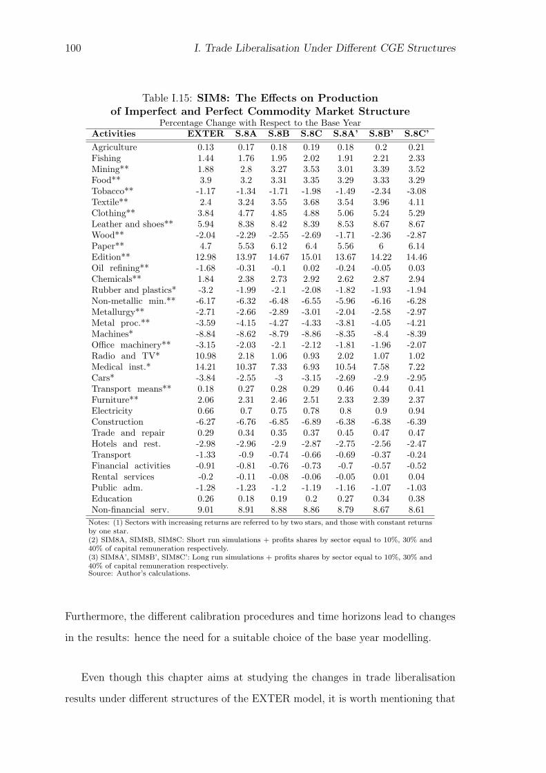
100 I. Trade Liberalisation Under Different CGE Structures

Table I.15: SIM8: The Effects on Productionof Imperfect and Perfect Commodity Market Structure

Percentage Change with Respect to the Base YearActivities EXTER S.8A S.8B S.8C S.8A’ S.8B’ S.8C’Agriculture 0.13 0.17 0.18 0.19 0.18 0.2 0.21Fishing 1.44 1.76 1.95 2.02 1.91 2.21 2.33Mining** 1.88 2.8 3.27 3.53 3.01 3.39 3.52Food** 3.9 3.2 3.31 3.35 3.29 3.33 3.29Tobacco** -1.17 -1.34 -1.71 -1.98 -1.49 -2.34 -3.08Textile** 2.4 3.24 3.55 3.68 3.54 3.96 4.11Clothing** 3.84 4.77 4.85 4.88 5.06 5.24 5.29Leather and shoes** 5.94 8.38 8.42 8.39 8.53 8.67 8.67Wood** -2.04 -2.29 -2.55 -2.69 -1.71 -2.36 -2.87Paper** 4.7 5.53 6.12 6.4 5.56 6 6.14Edition** 12.98 13.97 14.67 15.01 13.67 14.22 14.46Oil refining** -1.68 -0.31 -0.1 0.02 -0.24 -0.05 0.03Chemicals** 1.84 2.38 2.73 2.92 2.62 2.87 2.94Rubber and plastics* -3.2 -1.99 -2.1 -2.08 -1.82 -1.93 -1.94Non-metallic min.** -6.17 -6.32 -6.48 -6.55 -5.96 -6.16 -6.28Metallurgy** -2.71 -2.66 -2.89 -3.01 -2.04 -2.58 -2.97Metal proc.** -3.59 -4.15 -4.27 -4.33 -3.81 -4.05 -4.21Machines* -8.84 -8.62 -8.79 -8.86 -8.35 -8.4 -8.39Office machinery** -3.15 -2.03 -2.1 -2.12 -1.81 -1.96 -2.07Radio and TV* 10.98 2.18 1.06 0.93 2.02 1.07 1.02Medical inst.* 14.21 10.37 7.33 6.93 10.54 7.58 7.22Cars* -3.84 -2.55 -3 -3.15 -2.69 -2.9 -2.95Transport means** 0.18 0.27 0.28 0.29 0.46 0.44 0.41Furniture** 2.06 2.31 2.46 2.51 2.33 2.39 2.37Electricity 0.66 0.7 0.75 0.78 0.8 0.9 0.94Construction -6.27 -6.76 -6.85 -6.89 -6.38 -6.38 -6.39Trade and repair 0.29 0.34 0.35 0.37 0.45 0.47 0.47Hotels and rest. -2.98 -2.96 -2.9 -2.87 -2.75 -2.56 -2.47Transport -1.33 -0.9 -0.74 -0.66 -0.69 -0.37 -0.24Financial activities -0.91 -0.81 -0.76 -0.73 -0.7 -0.57 -0.52Rental services -0.2 -0.11 -0.08 -0.06 -0.05 0.01 0.04Public adm. -1.28 -1.23 -1.2 -1.19 -1.16 -1.07 -1.03Education 0.26 0.18 0.19 0.2 0.27 0.34 0.38Non-financial serv. 9.01 8.91 8.88 8.86 8.79 8.67 8.61

Notes: (1) Sectors with increasing returns are referred to by two stars, and those with constant returnsby one star.(2) SIM8A, SIM8B, SIM8C: Short run simulations + profits shares by sector equal to 10%, 30% and40% of capital remuneration respectively.(3) SIM8A’, SIM8B’, SIM8C’: Long run simulations + profits shares by sector equal to 10%, 30% and40% of capital remuneration respectively.Source: Author’s calculations.

Furthermore, the different calibration procedures and time horizons lead to changes

in the results: hence the need for a suitable choice of the base year modelling.

Even though this chapter aims at studying the changes in trade liberalisation

results under different structures of the EXTER model, it is worth mentioning that

101

Table I.16: SIM8: Perceived Price Elasticity of Domestic DemandPercentage Change with Respect to the Base Year

Activities SIM8A SIM8B SIM8C SIM8A’ SIM8B’ SIM8C’Mining** 0.14 0.10 0.08 0.13 0.09 0.08Food** 0.49 0.48 0.48 0.48 0.47 0.47Tobacco** 0.08 0.08 0.08 0.08 0.09 0.10Textile** -0.21 -0.25 -0.26 -0.22 -0.26 -0.27Clothing** -0.13 -0.14 -0.15 -0.14 -0.15 -0.15Leather and shoes** -0.13 -0.15 -0.16 -0.13 -0.15 -0.16Wood** 0.21 0.21 0.22 0.18 0.22 0.25Paper** 0.43 0.37 0.35 0.42 0.36 0.34Edition** -0.02 -0.06 -0.08 -0.03 -0.08 -0.10Oil refining** -0.02 -0.02 -0.03 0.00 0.00 0.00Chemicals** 0.21 0.17 0.16 0.20 0.17 0.16Rubber and plastics* 0.62 0.60 0.59 0.63 0.60 0.60Non-metallic minerals** 0.24 0.25 0.26 0.24 0.27 0.28Metallurgy** 0.09 0.11 0.13 0.05 0.12 0.16Metal processing** 0.07 0.06 0.06 0.06 0.07 0.08Machines* -0.11 -0.12 -0.13 -0.11 -0.12 -0.12Office machinery** -0.09 -0.10 -0.10 -0.07 -0.07 -0.06Radio and TV* -0.12 -0.13 -0.13 -0.11 -0.12 -0.12Medical instruments* -0.07 -0.08 -0.08 -0.07 -0.09 -0.09Cars* 0.30 0.29 0.28 0.32 0.30 0.30Other transport means** -0.19 -0.20 -0.21 -0.20 -0.20 -0.20Furniture** 0.05 0.03 0.02 0.05 0.02 0.01

Notes: (1) Sectors with increasing returns are referred to by two stars, and those with constant returns by one star.(2) SIM8A, SIM8B, SIM8C: Short run simulations + profits shares by sector equal to 10%, 30% and 40% of capitalremuneration respectively.(3) SIM8A’, SIM8B’, SIM8C’: Long run simulations + profits shares by sector equal to 10%, 30% and 40% of capitalremuneration respectively.Source: Author’s calculations.

Morocco, like other developing countries, is subject to various barriers to foreign

competition (high tariff rates, quantitative restrictions...) and barriers to firm

entries (complex administrative mechanisms, absence of antitrust policies, small

local market, underdeveloped capital markets...). Imperfect competition is then an

appropriate market structure for such countries. In addition, in developing countries,

the domestic market is small reflecting unexploited scale economies. This inefficiency

is exacerbated by policies that encourage local producers to invest. Given the low

utilisation of productive capacity, efficiency gains resulting from increasing the scale

of local production are even more important.

2.4 Dynamic vs. Static

SIM9: Time Dimension

102 I. Trade Liberalisation Under Different CGE Structures

Table I.17: SIM8: Imperfect Commodity Market Structure,Some Selected Results

Percentage Change with Respect to the Base YearActivities Prof. Var. Firms Prof. Var. Firms

Cap. Numb. Cap. Numb.S.8A S.8A S.8A S.8A’ S.8A’ S.8A’

Mining** -9.1 0 0 0 0.39 -2.25Food** -28.33 0 0 0 5.59 -2.99Tobacco** -23.55 0 0 0 0.13 -1.29Textile** -7.65 0 0 0 0.42 -0.99Clothing** -3.16 0 0 0 0.16 -0.38Leather and shoes** -22.29 0 0 0 1.54 -1.22Wood** -34.32 0 0 0 1.71 -9.04Paper** -7.21 0 0 0 0.47 -1.36Edition** 26.66 0 0 0 -1.64 3.29Oil refining** -67.75 0 0 0 0.93 -1.48Chemicals** -20.41 0 0 0 1.07 -3.3Rubber and plastics* -32.21 0 0 0 0 -9.2Non-metallic minerals** -48.58 0 0 0 2.29 -9.39Metallurgy** -42.34 0 0 0 2.28 -9.14Metal processing** -62.8 0 0 0 4.61 -7.38Machines* -25.6 0 0 0 0 -11.39Office machinery** -87.97 0 0 0 6.8 -6.74Radio and TV* -62.36 0 0 0 0 -33.5Medical instruments* -0.67 0 0 0 0 -0.83Cars* -127.12 0 0 0 0 -5.89Other transport means** -25.14 0 0 0 1.39 -3.85Furniture** -18.21 0 0 0 0.78 -1.96Notes: (1) Sectors with increasing returns are referred to by two stars, and those with constant returnsby one star.(2) SIM8A, SIM8B, SIM8C: Short run simulations + profits shares by sector equal to 10%, 30% and40% of capital remuneration respectively.(3) SIM8A’, SIM8B’, SIM8C’: Long run simulations + profits shares by sector equal to 10%, 30% and40% of capital remuneration respectively.Source: Author’s calculations.

Until the midst of the 90s, CGE models dealing with trade policies were operating

in a static framework, excluding accumulation effects as well as the transition path

of the economy where short run policy impacts are likely to be different from those

of the medium and long run. Despite the theoretical and empirical evidence on the

benefits of trade liberalisation, the majority of these models have found that welfare

gains were less than 1% of GDP (Srinivasan and Whalley, 1986). This is mainly

imputed to the fact that static models do not capture the dynamic gains from trade

liberalisation. The simulation is run in a static comparative framework where the

new situation is viewed as an approximation of the long run equilibrium. However,

103

the convergence process is interesting because it is likely to entail welfare costs,

that are difficult to be ignored from a social point of view. Indeed, when assessing

the impact of trade liberalisation on Tunisia, Annabi and Rajhi (2001) show that

the static version of the model underestimates the impact of trade liberalisation

on production and welfare because it excludes the accumulation effects. Therefore,

economists became aware of the need for dynamic CGE models to assess the impact

of various trade policies.

Dynamic CGE models are twofold: sequential (recursive) and intertemporal.

Intertemporal models are based on optimal growth theory where the behaviour

of economic agents is characterised by perfect foresight. They know everything

about the future and react to future changes in prices. Households maximise

their intertemporal utility function under a wealth constraint to determine their

consumption schedule over time. Investment decisions by firms are the results of cash

flow maximisation over the whole time horizon. By contrast, a sequential dynamic

CGE model is a series of static models linked between periods by adjustment

procedures. MIRAGE belongs to the recursive dynamic family. The modification of

the static structure of EXTER according to MIRAGE dynamic structure involves

the addition of adjustment procedures for the first period exogenous variables:

Firstly, the capital stock of private sectors KDps adjusts between periods by the

means of capital depreciation rate and investment demand by sector:

KDps,t+1 = (1− depps)KDps,t + INV Dps,t

where depps is the capital depreciation rate of private sector ps18 and INV Dps,t

investment by destination of this sector at period t. For investment demand by

sector, I adopt the quadratic form proposed by Bourguignon et al. (1989):

INV Dps,t

KDps,t

= D1ps(rps,t

PINVt(it + depps))2 +D2ps(

rps,tPINVt(it + depps)

)

18 The annual depreciation rate of capital is fixed at 5.4% for Morocco (Zouhar, 2005).

104 I. Trade Liberalisation Under Different CGE Structures

where D1ps and D2ps are scale parameters, rps,t the rental rate of capital in sector

ps at period t, it the interest rate at period t (exogenous) and PINV the aggregate

price of investment given by:

PINVt =∏i

(PCi,tµi

)µi

PINV is the dual price of a Cobb-Douglas investment function, with µi being the

share of product i in total investment. With the introduction of investment by

sectors and the equation of capital accumulation, the calibration of the capital

stock must be adjusted. I assume that the sectoral growth rate of capital

INV Dps,0/KDps,0 is equal to the sum of the depreciation rate of capital and

population growth rate19. Since capital demand is endogenous in public sectors,

investment is then determined by the model:

INV Dpub,t = KDpub,t+1 −KDpub,t

The sum of investment by destination of private and public sectors must be equal

to the gross fixed capital formation ITV OL given by the ratio of total investment

value IT and the aggregate price of investment:

ITV OLt = ITt/PINVt

However, by constraining the sum of investment by destination of all sectors to be

equal to total investment volume, the model contains an extra equation. A free

variable needs to be introduced to the model in order to be squared. In addition,

the savings-driven determination of investment states that investment adjusts in

order to achieve the investment-savings equilibrium. Therefore, the free adjustment

19 This assumption implies the steady state condition for capital accumulation that is used inintertemporal models.

105

variable SI is introduced in the gross fixed capital formation equation:

ITV OLt = SIt(∑ps

INV Dps,t +∑pub

INV Dpub,t)

Now, with the adjustment of total investment volume, the investment-savings

equilibrium can be accomplished.

Secondly, labour supply LS is adjusted between periods according to an exogenous

annual growth rate assumed to be equal to the population natural growth rate gLS20:

LSt+1 = LSt(1 + gLS)

Thirdly, it is also possible to add updating mechanisms for other variables, such as

public expenditures, transfers, technological change or debt accumulation.

Before proceeding to the analysis, it is important to note that in a dynamic

model, the economy grows between periods even in the absence of any shock, due to

the updating mechanisms of the first-period exogenous variables. This growth path

of the economy without any shock is called “Business As Usual” (BAU). How does

the economy react to the updating mechanisms over periods?

On the one hand, the growing population induces, ceteris paribus, a higher level

of household consumption and thus affects upward the demand addressed to sectors.

On the other hand, the capital accumulation process increases the volume of capital

allocated to the different sectors. Given the relative substitutability between labour

and capital in the value added, more capital generates a higher production level.

However, the volume of production by sector exceeds the level of demand so that

producers lower their prices in order to sell more. Given that other things are

equal, lower prices for investment products motivate capital accumulation. As well,

lower input prices encourage firms to produce more. In sum, real GDP average

annual growth rate is about 1.6%. Growing production helps satisfy the increasing

20 gLS is set to 1.6% for Morocco (World Development Indicators Database 2001, the World Bank).

106 I. Trade Liberalisation Under Different CGE Structures

domestic demand, but also, since domestic prices fall, producers are motivated to

export. Given that other things are equal, imports must increase in order to keep

external savings constant.

Following production growth, labour demand increases. Consequently, the wage

rate must adjust upward in order to balance the market. However, the wage rate

being equal to the product of the physical marginal productivity of labour and

the average value added price, the drop of the latter is sufficient to decrease the

wage rate between periods. But the wage payroll increases because labour supply

also grows between periods. Since labour remuneration constitutes the principal

source of household income, the latter increases and household welfare improves

over time. Welfare improvement reaches 28% of household disposable income in the

last period of the model (20 periods). Concerning capital remuneration, massive

investment increases the volume of capital relatively to labour, and reduces the

marginal productivity of capital, as well as the rental rate of capital by sector.

However, given the increasing volume of capital allocated to sectors, total capital

remuneration increases. Mainly affected by capital remuneration, firms’ income

grows and so does government income. The latter also collects more sales tax due to

higher consumption, as well as more direct taxes. Following income growth, savings

also increase, and so does the gross fixed capital formation.

When the trade liberalisation shock is simulated, the economy will have another

growth path, due to simultaneous effect of the shock and the updating mechanisms

of the first-period exogenous variables. Consequently, the analysis should be done

with respect to the BAU growth path. In other words, the value of a given variable

at period t after the shock should be compared to its value at period t before the

shock.

Among the seventeen contracting sectors in the static model, ten are added to

winners in the medium and long run: tobacco and rubber sectors, oil refining, metal

processing, office machinery, car industry, transport, financial and rental services,

education (Table I.18). This is explained by different reasons: first of all, capital

107

accumulation is motivated by lower prices of investment products after tariff removal.

The capital accumulation process helps increase sectoral production. The continuous

expansion of the originally expanding sectors raises intermediary input demand

addressed to all sectors, including the contracting ones. Secondly, the growing

population induces a rise of household consumption, that in turn, positively affects,

ceteris paribus, the demand addressed to sectors. In order to meet the increasing

demand with respect to the static model, the above-mentioned sectors expand in

the medium and long run.

In the static model, trade liberalisation boosted imports, with some exceptions.

Imports of oil refining products, metallurgy, metal processing, machines, office ma-

chinery, other transport means, hotels and restaurants, transport services, financial

and rental services decreased due to lower domestic demand. Imports of fishery

and clothing products, radio and television also decreased, because local production

replaced imports. In the long run simulation, increasing demand motivated by

household consumption and intermediary input demand boosts imports in some of

the above-mentioned sectors, mainly: fishery, clothing, oil refining, metallurgy, metal

processing, office machinery, radio and TV, other transport means, transport and

financial services. By contrast, exports evolve in the same direction in the short and

long run.

When sectors expand, they need more production factors. For a given period,

increased labour demand creates a pressure on labour market that drives the wage

up, in presence of fixed labour supply. That is why the wage rate increases

in the medium and long run, after being decreasing in the static model. Since

labour remuneration mainly affects household income, when the wage rate increases,

household income also does, by contrast to the static model.

While trade liberalisation leads, during the first period, to a contraction of the

overall activity by 3.96%, this negative impact vanishes, starting period 5. The

overall activity grows by 0.34% at the twentieth period of the model. Furthermore,

welfare improvement increases with time and accounts for 0.39% of household

108 I. Trade Liberalisation Under Different CGE Structures

Table I.18: SIM9: The effects on Productionof the Static and Dynamic Structures

Percentage Change with Respect to the BAU Growth Path.Activities EXTER SIM9 SIM9 SIM9 SIM9 SIM9

t t+5 t+10 t+15 t+20Agriculture 0.13 0.03 2.46 4.85 6.68 8.13Fishing 1.44 1.39 3.56 5.35 6.63 7.62Mining 1.88 1.23 2.58 3.55 4.13 4.52Food 3.90 3.75 6.32 8.46 10.03 11.28Tobacco -1.17 -0.86 -1.10 -0.69 0.01 0.79Textile 2.40 2.68 5.82 8.58 10.49 11.83Clothing 3.84 3.70 7.24 10.28 12.32 13.70Leather and shoes 5.94 5.57 8.77 11.08 12.55 13.58Wood -2.04 -1.47 -1.80 -1.64 -1.17 -0.59Paper 4.70 1.54 4.07 6.14 7.57 8.62Edition 12.98 3.57 6.80 9.46 11.22 12.44Oil refining -1.68 -0.92 0.06 1.14 2.02 2.80Chemicals 1.84 1.83 4.42 6.39 7.71 8.70Rubber and plastics -3.20 -2.64 -1.01 0.37 1.44 2.32Non-metallic minerals -6.17 -4.49 -5.35 -5.52 -5.21 -4.72Metallurgy -2.71 -2.02 -3.00 -3.07 -2.69 -2.17Metal processing -3.59 -2.22 -1.58 -0.80 -0.03 0.70Machines -8.84 -6.67 -5.79 -4.93 -4.11 -3.34Office machinery -3.15 -1.41 -0.96 -0.44 0.12 0.69Radio and TV 10.98 11.48 18.93 25.87 31.97 37.83Medical instruments 14.21 9.49 16.66 21.87 25.17 27.50Cars -3.84 -1.88 -0.59 0.54 1.50 2.35Other transport means 0.18 0.38 1.48 2.27 2.84 3.31Furniture 2.06 1.54 3.84 5.72 7.11 8.23Electricity 0.66 0.46 2.14 3.60 4.74 5.70Construction -6.27 -4.23 -4.99 -5.09 -4.74 -4.21Trade and repair 0.29 0.46 2.54 4.42 5.89 7.13Hotels and rest. -2.98 -1.99 -2.16 -1.70 -1.01 -0.27Transport -1.33 -0.86 -0.31 0.30 0.88 1.43Financial activities -0.91 -0.59 0.17 1.21 2.15 3.00Rental services -0.20 -0.15 0.89 1.93 2.85 3.70Public administration -1.28 -0.96 -1.05 -1.16 -1.27 -1.37Education -0.01 -0.01 0.11 0.24 0.37 0.50Non-financial services 9.01 0.51 2.98 5.81 8.17 9.98Notes: For EXTER, percentage change with respect to the base year. EXTER and period t ofSIM9 lead to slightly different results because the calibration of the base year capital volume isdifferent in the static and dynamic models.Source: Author’s calculations.

disposable income after 20 years. To put it in a nutshell, this exercise supports

the scientific belief that the time dimension is crucial for analysing the effects of

trade liberalisation.

109

3 Conclusion

This chapter is an attempt to assess the sensitivity of trade liberalisation results

to changes in a CGE model structure. Tariff removal is first simulated on a small

open economy model, EXTER, applied to the Moroccan SAM. Then the results of

trade liberalisation are analysed for every change in EXTER assumptions, based on

IFPRI, GTAP and MIRAGE models. As expected, the change of the numeraire

only modifies values, all volumes being equal to the benchmark model. The

results are not considerably affected when the functional form of production (CES

instead of Leontief), value added (CES instead of Cobb-Douglas), investment volume

(CES instead of Cobb-Douglas) and utility function (Stone-Geary instead of Cobb-

Douglas) are modified: only the classification of winners and losers is altered as well

as the magnitude of variable changes. They are, however, more sensitive to changes

in the intermediate consumption Leontief function as well as to the macroeconomic

closure, the commodity market structure and the time horizon adopted. Many

changes are detected in signs. Hence it is crucial to accurately identify the problem in

order to determine the most appropriate analytical framework for the corresponding

economy.

The experience gained in this chapter concerning CGE model behaviours under

different structures helps conceptualise the appropriate CGE models for assessing

the impact of migration on Morocco. To begin with, a static CGE model was built,

based on the conclusions of this chapter, in order to deal with the first question asked

in this thesis, about the simultaneous impact of inflows and outflows of workers on

the labour market of the sending country. Chapter 2 investigates this issue with a

particular attention to the effect of migratory flows on unemployment in Morocco.

110 I. Trade Liberalisation Under Different CGE Structures

I.A Appendix A: Data

The SAM constitutes the empirical database required to satisfy the accounting

coherence of a CGE model. I use the Moroccan SAM built by Abdelkhalek and

Zaoujal (2004) for the year 1998 from several Moroccan data sources: the input-

output table of the Moroccan economy for 1998, built by the Direction of Statistics

and published, in a preliminary version, in 2002, the National Survey on Household

Living Standards (NSHLS) in 1998-1999 carried out by the Direction of Statistics,

documents from the Ministry of Economy and Finance, from External Trade

department, from the Ministry of Agriculture, from Foreign Exchange department,

and from Bank Al-Maghrib. The SAM gathers two production factors (labour and

capital), four types of agents (households, firms, government, the RoW), 34 sectors

of activity that match exactly those of the input-output table of the Moroccan

economy in 1998.

The SAM describes the Moroccan economy in 1998. At this period, GDP

amounted to MAD 344 billion. On the output side, the primary and secondary

sector are relatively small accounting for respectively 16.4% and 29.4% of real

GDP. By contrast, the tertiary sector accounts for 54.2% of real GDP. On the

demand side, households consumption accounts for 68% of GDP, while government

current expenditures account for 18% of GDP. At the same time, total investment

expenditures represent 22% of GDP, implying that Morocco is running a trade

deficit equivalent to 8% of GDP. Indeed, exports and imports represent respectively

23% and 31% of GDP. Industrial imports constitute 80% of total imports whereas

agricultural products and services only account for 8% and 12% of total imports,

respectively. Industrial exports are also the most important, about 81% of total

exports, followed by services that represent 11% of total exports whereas agricultural

products only account for 8% of total exports.

Income elasticities are based on estimates by the Economic Research Service,

US Department of Agriculture from the International Comparison Project Data of

111

the World Bank in 1996 (Bernstein et al., 2003). Elasticities are estimated for

the following product groups: food, beverages and tobacco (0.65), clothing and

footwear (0.916), fuel and power (1.206), house operations (1.202), medical care

(1.375), education (1.076), transport and communication (1.219), recreation (1.503),

Other (1.361). For food, the elasticities are estimated for breads and cereals (0.452),

meat (0.694), fish (0.793), dairy (0.757), fats and oils (0.472), fruits and vegetables

(0.563), and other foods (0.691).

112 I. Trade Liberalisation Under Different CGE Structures

I.B Appendix B: Sectoral Aggregation

AGR AgricultureFIS FishingMII Mining industryFOO Food industryTOB Tobacco industryTEX Textile industryCLO Clothing industryLEA Leather and shoes industryWOO Fabrication of wood and wood-based productsPAP Paper industryEDI Edition, printing and reproductionOIL Oil refiningCHE Chemical industryRUB Rubber and plastic industryMIN Manufacture of other non-metallic mineral productsMET MetallurgyMEP Metal processingMAC Machines and equipmentsOFF Office machineryRAD Radio and TV equipmentsMED Medical instrument manufacturingCAR Car industryMTR Manufacture of other transport meansFUR Furniture manufacturing, other industriesELE Electricity and water - production and distributionCON ConstructionTRR Trade and repairHOT Hotels and restaurantsTRA Transport and telecommunicationFIN Financial activities and insuranceREN Rental servicesADM Public administration and social securityEDU Education and healthSER Other non-financial services

113

I.C Appendix C: Mathematical Statement of the

Model

Set indices are given by lower-case Latin letters as subscripts to variables and

parameters. Parameters are represented with lower-case Latin letters or lower-case

Greek letters, endogenous variables with upper-case Latin letters without a bar,

exogenous variables with upper-case Latin letters with a bar.

Sets

j ∈ J Sectorsi ∈ I Products (=J)tr ∈ TR ⊂ J Tradable sectorsntr ∈ NTR ⊂ J Non-tradable sectorsps ∈ PS ⊂ J Private sectorspub ∈ PUB ⊂ J Public sectorsag ∈ AG Agents (“hh”=households, “fm”=firms, “gv”=government,

“row”=RoW)

Parameters

vj Share of value added in the Leontief production function of sector jioj Share of intermediary consumption in the Leontief production function

of sector jaijij Intermediary consumption of good i by unit of production of sector jAps Scale parameter of the Cobb-Douglas value added function of sector psαps Elasticity of value added with respect to labour demand in sector pslpub Share of labour in the Leontief value added function of public sector pubkpub Share of capital in the Leontief value added function of public sector pubϕ Household’s propensity to saveγi Budgetary share of good i in household incomeµi Share of product i in total investmenttxj Indirect taxes on product jtmtr Import tariff rate on product trtetr Export tariff rate on product trtyh Direct tax rate on household incometyf Direct tax rate on firms’ income

114 I. Trade Liberalisation Under Different CGE Structures

Amtr Scale parameter of the Armington CES functionθtr Share parameter of the Armington CES functionσtr Elasticity of substitution (Armington function)ρtr Substitution parameterBetr Scale parameter of the CET production functionβtr Share parameter of the CET production functionτtr Transformation elasticity (CET production function)κtr Transformation parameterηag Share of labour remuneration received by agent agλag Share of capital remuneration received by agent agδj Share of sector j’s value added in GDP at factor cost

Endogenous variables

a) Prices

w Average wagerj Capital return in sector jPVj Value added price of sector jPCj Composite price of product jPj Producer price of product jP lj Producer price of product j sold on the domestic marketPDj Market price of product j sold on the domestic marketPMtr Domestic price of the imported good trPEj Producer price of the exported good trPwmtr International import price of product tr, in foreign currencyPwetr International export price of product tr, in foreign currencye Nominal exchange rate (the price of a unit of foreign currency in

domestic currency), numerairePindex GDP deflator

b) Production

V Aj Value added of sector j (volume)XSj Production of sector j (volume)CIj Total intermediary consumption of sector j (volume)DIi,j Intermediary demand of product i by sector j (volume)LDj Labour demand by sector j (volume)KDj Capital demand by sector j (volume)LS Labour supply

c) Income/Savings

Yag Agent ag’s income

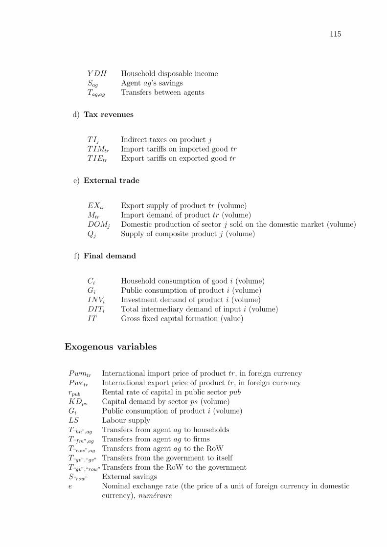
115

Y DH Household disposable incomeSag Agent ag’s savingsTag,ag Transfers between agents

d) Tax revenues

TIj Indirect taxes on product jTIMtr Import tariffs on imported good trTIEtr Export tariffs on exported good tr

e) External trade

EXtr Export supply of product tr (volume)Mtr Import demand of product tr (volume)DOMj Domestic production of sector j sold on the domestic market (volume)Qj Supply of composite product j (volume)

f) Final demand

Ci Household consumption of good i (volume)Gi Public consumption of product i (volume)INVi Investment demand of product i (volume)DITi Total intermediary demand of input i (volume)IT Gross fixed capital formation (value)

Exogenous variables

Pwmtr International import price of product tr, in foreign currencyPwetr International export price of product tr, in foreign currencyrpub Rental rate of capital in public sector pubKDps Capital demand by sector ps (volume)Gi Public consumption of product i (volume)LS Labour supplyT“hh”,ag Transfers from agent ag to householdsT“fm”,ag Transfers from agent ag to firmsT“row”,ag Transfers from agent ag to the RoWT“gv”,“gv” Transfers from the government to itselfT“gv”,“row” Transfers from the RoW to the governmentS“row” External savingse Nominal exchange rate (the price of a unit of foreign currency in domestic

currency), numeraire

116 I. Trade Liberalisation Under Different CGE Structures

Equations

Production

XSj =V Ajvj

(A1)

V Aps = ApsLDαpsps KDps

(1−αps)(A2)

KDpub = kpubV Apub (A3)

CIj = iojXSj (A4)

DIij = aijijCIj (A5)

LDps =αpsPVpsV Aps

w(A6)

LDpub = lpubV Apub (A7)

KDpub =PVpubV Apub − wLDpub

rpub(A8)

Households and Firms

Y“hh” = (1− η“fm” − η“gv” − η“row”)w∑j

LDj + λ“hh”

∑j

rjKDj +∑ag

T“hh”,ag(A9)

Y DH = Y“hh” −∑ag

T ag,“hh” (A10)

Y“fm” = η“fm”w∑j

LDj + (1− λ“hh” − η“gv” − η“row”)∑j

rjKDj +∑ag

T“fm”,ag(A11)

S“hh” = ϕY DH (A12)

S“fm” = Y“fm” −∑ag

T ag,“fm” (A13)

117

The Government

TItr = txtr(PtrXStr − PEtrEXtr) + txtr(1 + tmtr)PwmtreMtr (A14)

TIntr = txntrPLntrXStr (A15)

TIMtr = tmtrPwmtreMtr (A16)

TIEtr = tetrPEtrEXtr (A17)

T“gv”,“hh” = tyhY“hh” (A18)

T“gv”,“fm” = tyfY“fm” (A19)

Y G = η“gv”w∑j

LDj + λ“gv”

∑j

rjKDj +∑tr

TIMtr +∑tr

TIEtr +∑j

TIj +∑ag

T “gv”,ag (A20)

S“gv” = Y“gv” −∑i

PCiGi −∑ag

Tag,“gv” (A21)

External Trade

XStr = Betr[βtrEX−κtrtr + (1− βtr)DOM−κtr

tr ]− 1κtr (A22)

XSntr = DOMntr (A23)

DOMtr

EXtr

= [(1− βtrβtr

)(PEtrPLtr

)]τtr (A24)

Qtr = Amtr[θtrM−ρtrtr

+ (1− θtr)DOM−ρtrtr ]

− 1ρtr (A25)

Qntr = DOMntr (A26)

Mtr

DOMtr

= [(θtr

1− θtr)(PDtr

PMtr

)]σtr (A27)

118 I. Trade Liberalisation Under Different CGE Structures

S“row” = e∑tr

PwmtrMtr + η“row”w∑j

LDj + λ“row”

∑j

rjKDj +∑ag

T“row”,ag − e∑tr

PwetrEXtr −∑ag

Tag,“row” (A28)

Final Demand

Ci = γiY DH/PCi (A29)

INVi =µiIT

PCi(A30)

DITi =∑j

DIij (A31)

Prices

PVj =PjXSj −

∑i PCiDIij

V Aj(A32)

rps =PVpsV Aps − wLDps

KDps

(A33)

PMtr = Pwmtre(1 + tmtr)(1 + txtr) (A34)

PEtr =Pwetre

(1 + tetr)(A35)

PDj = Plj(1 + txj) (A36)

PCtr =PDtrDOMtr + PMtrMtr

Qtr

(A37)

PCntr = PDntr (A38)

Ptr =PLtrDOMtr + PEtrEXtr

XStr(A39)

Pntr = PLntr (A40)

119

Pindex =∑j

PVjδj (A41)

Equilibrium Conditions and Closure

LS =∑j

LDj (A42)

Qi = DITi + Ci + INVi +Gi (A43)

IT =∑ag

Sag (A44)

EV = (

∏i PCOi∏i PCi

)γi

Y DH − Y DHO (A45)

Chapter II

Is International Migration a Cure

for Moroccan Unemployment?1

Unemployment, which represented less than 17% of the economic causes of Moroccan

emigration before 1960, far behind the search for a more lucrative work (50%) or

the improvement of the living standards (25%), became the principal economic

cause of emigration in the 1990s. According to the data collected by Hamdouch

(2000), 41% of answers indicate unemployment as the first cause of emigration,

whereas the search for a more lucrative work and the improvement of the standard

of living represent 38% and 14% respectively of the reasons for emigration. In this

context, dealing with the impact of migration on Moroccan unemployment becomes

an interesting question.

The relation between migration and economic development of the sending

country has not been correctly addressed for a long time, primarily due to scarce

reliable data on migratory flows and migrants characteristics at the macroeconomic

level as well as the microeconomic one2. In the majority of the cases, studies have

1 This chapter is a new version of a joint paper with B. Decaluwe (Karam and Decaluwe, 2008).2 Fortunately, databases become increasingly available, like the one of Docquier and Marfouk

(2004) on brain drain.

121

122 II. Is International Migration a Cure for Moroccan Unemployment?

mainly analysed the impact of migration on the country of destination3, and in very

rare occasions on the country of origin. Only a limited number of studies address the

impact of migration (directly or indirectly through remittances) on inequality and

wages, growth and welfare, its social effects (children health, education, women’s

role...), or the impact of returned migrants who acquired experience in the host

country, as well as the relation between migration and trade4. The “brain drain”

and “brain gain” were also the issue addressed by several works.

The very few studies that try to encircle in a systematic way the impact of

migration on labour market are limited to the effect of international migration on

unemployment in developing countries. However, labour mobility could be observed

in several directions. For instance, a transitory South-South migration from a

developing country towards another one, before migrating to a developed country,

can coexist with internal migration from rural to urban areas, or emigration to more

developed countries5. The combination of these forces is able to exert unexpected

effects on the labour market, and in order to understand them and study their

consequences, I choose the Moroccan case. Indeed, Morocco seems the typical

example of a developing country undergoing the combination of different migratory

flows: rural and urban emigration towards the EU, internal migration from rural to

urban areas, and finally Sub-Saharan immigration to Morocco for transit to Europe

or in order to definitely stay there.

A sketchy analysis suggests that on the one hand, urban emigration reduces

urban unemployment and increases wages, whereas internal migration and Sub-

Saharan immigration to the cities raise the pressure on urban labour market. How-

ever, the simultaneous impact of these different forces on labour market conditions

cannot be predicted without ambiguity since it depends on the magnitude of each

migratory flow and the initial conditions of labour market. If internal migration to

3 For a review of the literature on the effects of migration on the destination country, see Drinkwateret al. (2003).

4 For a review of the literature on the effects of migration on the sending country, see Katseli etal. (2006).

5 Emigration is the act of leaving one’s native country or region to settle in another. By contrast,immigration is the entry of foreigners into a country to stay and work there.

123

urban areas and Sub-Saharan immigration to Morocco dominate urban emigration,

urban unemployment rate must increase. Conversely, if urban emigration overrides

internal migration and Sub-Saharan immigration, unemployment rate will probably

decrease.

In order to take simultaneously into account the existing forces, I build a static

CGE model. This tool allows to endogenise the determinants of migratory flows

and to capture their coexisting direct effects on urban labour market, particularly

on unemployment, and their direct and indirect effects on the remainder of the

economy. Contrary to other studies on this question6, I do not think that an

aggregate approach is sufficient to seize the complexity of the existing mechanisms,

and this is why I undertake a fine disaggregation by professional category. Such a

fine description of the labour market that takes into account unemployment rates by

professional category is justified by the fact that emigration and immigration do not

affect all categories in the same way. In other terms, it allows to seize the impact of

migration on each segment of labour market.

The chapter is structured as follows. Section 1 highlights some characteristics of

Moroccan labour market. The theoretical framework is presented in Section 2. In

Section 3, I run three simulations, the first one consisting of a 10% fall in migration

costs, the second of a 10% rise of Sub-Saharan immigrant stock, and finally, the

simultaneous effects of the two previous shocks. Section 4 concludes and discusses

the policy implications of this study.

1 Moroccan Labour Market

As pointed out earlier, the Moroccan labour market is simultaneously affected by

inflows and outflows of workers. Data on international migration come from OECD

(2006) while data on internal migration and Sub-Saharan immigration are taken

from empirical studies.

6 See for example Agenor and El Aynaoui (2003).

124 II. Is International Migration a Cure for Moroccan Unemployment?

OECD data indicate that the traditional destinations of Moroccan migrants, such

as Belgium, France, Spain, Italy, and the Netherlands, continue to receive important

migratory flows. In 2004, 8,000 Moroccans entered to Belgium, 21,700 to France,

24,600 to Italy, 3,300 to the Netherlands and 58,800 to Spain. Accounting for 21.5%

of the foreign population living in Spain in 2002, they are considered as the largest

foreign community in this country. Moreover and according to an opinion of the

International Organisation of Migration, Moroccan migration towards the EU is

mostly originated from rural areas (Erf and Heering, 2002).

Internal migration is motivated by climatic risks associated to agricultural

production that encourage farmers to look for a stable employment in urban areas in

order to mitigate the great fluctuations of their agricultural income. The available

estimations indicate that, approximately 200,000 migrants move annually into urban

areas, which is equivalent to 40% of the total increase in urban population (Agenor

and El Aynaoui, 2003).

Clandestine migration from Sub-Saharan Africa proliferated since the beginning

of the 1990s due to the fragility of this continent. Poverty exacerbation, natural

resource shortages (water in particular), conflicts and wars of any nature encourage

African immigrants to transit by Morocco to Spain and Europe7 or to settle definitely

in Morocco in order to profit from its stability and prosperity. One of the more

important consequences of illegal immigration on Morocco is that an increasingly

significant number of Sub-Saharan immigrants, scalded by the difficulties they meet

on the migratory way leading them to Europe, choose finally to stay in Morocco

(mainly in urban areas). Data on Sub-Saharan immigration are scarce and their

collection is difficult because the vast majority of African immigrants are clandestine.

According to Lahlou (2003), there would be between 6,000 and 15,000 irregular

migrants. I retain the upper bound.

7 The transit by Morocco is explained by geographical reasons (Morocco being at 14 km of theSpanish coast), as well as historical, cultural, religious, and socio-economic reasons like thepossibility to work on spot all along the migratory way.

125

I deal here with the characteristics of Moroccan labour market8. In this model,

the Moroccan labour market is divided in two segments: rural and urban, each

one composed of ten sub-segments by professional category. National employment

is roughly equally distributed between rural and urban areas. In 2005, urban

employment accounted for 50.5% of national employment. This percentage slightly

changes over time.

Table II.1: Employment by Activity, in 2005 (%)Sectors National Rural UrbanAgriculture 45.5 80.2 5.2Industry 12.4 3.9 22.3Services 26 8.8 45.9Construction 7.1 5.2 9.3Public sector 9 1.9 17.3Source: Royaume du Maroc (2005).

The structure of employment by activity (Table II.1) shows the relatively

important weight of agriculture. In 2005, this sector, absorbing 45.5% of national

employment, predominates in rural areas, with 80.2% of total rural employment,

and is particularly based on family work. The service sector absorbs 26% of

national employment and is the principal provider of urban employment (45.9%).

The industrial sector only accounts for 12.4% of total employment, 3.9% in rural

areas and 22.3% in urban areas. The construction sector employs 7.1% of total

labour, 9.3% in urban areas and 5.2% in rural areas. Employment opportunities

come principally from the private sector, absorbing 91% of total employment at the

national level, 98% in rural areas and 83% in urban areas. The public sector mainly

employs urban workers, with 17.3% of urban employment against only 1.9% in rural

areas.

The distribution of Moroccan working population by professional category

(Table II.2) shows that “farm labourers” is the most exerted profession at the

8 Illustrative figures are taken from the Royaume du Maroc (2005a). Employment is distributedbetween professional categories according to the Analytical Nomenclature of Professions estab-lished by the Direction of Statistics (Royaume du Maroc, 2001).

126 II. Is International Migration a Cure for Moroccan Unemployment?

Table II.2: Employment by professional category, in 2005 (%)Professions National Rural UrbanDirectors 0.8 0.1 1.6Senior executive 1.1 0 2.4Junior staff 3.6 0.4 7.2Employees 7.9 1.6 15.2Commercial intermediaries 7.5 3.3 12.4Farmers 12.4 21.6 1.7Craftsmen 16.3 6.6 27.5Farm labourers 32.6 58.1 3.2Drivers 3 1.3 5Warehousemen 14.8 7 23.8

Notes: For the complete headings of professions, see Appendix B.Source: Royaume du Maroc (2005).

national level. Then come the categories “craftsmen” and “warehousemen”. The

category “workmen” is also the biggest in rural areas followed by the categories

“farmers”, “warehousemen” and “craftsmen”. In urban areas, the category “farm

labourers” only accounts for 3.2% of urban employment. The category “craftsmen”

is henceforth ranked first followed by “warehousemen”, “employees” and “commercial

intermediaries”.

Table II.3: Unemployment rates by professional category, in 2005Professions NationalDirectors 2.2Senior executive 1.7Junior staff 6.1Employees 11.2Commercial intermediaries 3.2Farmers 0.3Craftsmen 10.1Farm labourers 2Drivers 8.5Warehousemen 12Source: Direction of Statistics, Rabat.

Like many developing countries, unemployment in Morocco is primarily an urban

phenomenon. Unemployment rate rose in 1999 to 22% then fell to 18.3% in 2005. By

contrast, rural unemployment rate is low, about 3.6% in 2005. At the national level,

127

unemployment rate reached 13.9% in 1999 then fell to 11% in 2005. In addition,

unpublished data provided by the Direction of Statistics, Rabat (Table II.3) show

that warehousemen, employees and craftsmen have the highest unemployment rates

(12%, 11.2% and 10.1% respectively). On the other hand, farmers and senior

executive exhibit the lowest rates (0.3% and 1.7% respectively).

2 Theoretical Framework

In order to correctly analyse the impact of migration on the different segments of

labour market, it is important to identify the origin of migratory flows. If one

thinks that Moroccan emigration from rural or urban areas relaxes the pressure on

the corresponding domestic labour markets, the drop in labour supply induces a rise

in rural or urban wages. Given that unemployment is an important characteristic

of urban labour market, emigration of urban workers, when it mainly affects some

professional categories, obviously reduces unemployment rates for these categories

and not for the others, if there is some degree of specificity in qualifications. On the

contrary, internal migration of rural workers and African immigration to urban areas

increase labour supply and unemployment rates of the different professions. Since

emigration and immigration do not touch the same categories, their impact will

be different from a market to another. It is also clear that the eventual labour

surplus on some segments of labour market will reduce wages (freely adjusting

or negotiated by the means of a wage convention). When these migratory flows

coexist, the ultimate effect on urban unemployment rates by professional category is

ambiguous. A fine modelling of labour market, illustrative of all these migratory

movements, is therefore necessary. The remainder of this section describes the

behavioural assumptions I retain.

The benchmark CGE model is a static real model of a small open economy,

inspired from Decaluwe et al. (2001) and developed by Cockburn et al. (2006).

This basic structure is however deeply modified in order to adequately describe the

128 II. Is International Migration a Cure for Moroccan Unemployment?

behaviour of labour market as well as the internal and external determinants of

migratory flows. Very briefly, my version of this model contains 34 mono-productive

sectors distributed between two aggregate sectors: a rural one (agriculture and

fishing) and an urban one (industry, tradable and non-tradable services); five agents

(rural and urban households, firms, government, and the RoW). I further modify

the specification of the rural sector in order to distinguish, within this sector,

between subsistence and industrial agriculture. The production process employs two

production factors: labour and capital. Because of the relative complementarity of

capital and labour in the public value added, it is now represented by a Leontief

function, on the contrary to the CES function of private value added. The capital

is sector-specific. Rural labour is a bundle of rural professional categories and each

rural labour category is perfectly mobile between rural sectors. Urban labour is also

a bundle of urban categories with each one being mobile between urban sectors, but

sub-segments of urban market are imperfect due to the existence of unemployment.

In addition, I endogenise the labour supply on each sub-segment of rural and urban

markets. I further assume that unemployed persons can not change their profession.

In other words, the cross elasticity of labour supply is null. Finally, I introduce a

new block of equations, relative to rural and urban emigration, internal migration

from rural to urban areas and Sub-Saharan immigration, and I suppose the existence

of migration costs. The model has an investment-driven closure: total investment

volume is fixed. Households and firms’ savings are determined by the model and

foreign savings are fixed. Uniform adjustments of the value added tax rate across

all sectors assure that government savings vary endogenously to achieve savings-

investment equilibrium9.

For the sake of brevity, I only describe here the migration block, the specification

9 However, the CGE literature on Morocco (Agenor et al., 2003; Lofgren et al., 1999) made use ofa savings-driven closure where government savings are a fixed proportion of GDP. In the presentcase, an investment-driven closure is preferable because the model is static and firms’ investmentdecisions rarely change in the short run. Nonetheless, I also run the simulations with a savings-driven closure: while this new closure is expected to generate different outcomes, as pointed outin Chapter 1, the results show that the signs of unemployment and wage changes are the sameas before. The results are available to the interested reader upon request.

129

of rural and public sectors as well as the endogeneisation of labour supply.

All equations can be examined in Appendix C. The model is calibrated on a

disaggregated SAM for 1998. Data on migration come from OECD (2006).

Appendix A and B present a detailed explanation of all data sources. The model

is implemented in GAMS (Brooke et al., 1988) and solved with NLP, a solver for

non-linear programming.

2.1 Migratory Flows

2.1.1 Migration Costs

When an individual migrates from a region to another or when he decides to

leave his country, this can not be done without costs. Any migratory movement

induces financial costs (travel cost, search for an apartment, search for a job...) and

psychological costs (change of the way of life, adaptation to a new culture and a new

community...) for the migrant. Migration costs are modelled a la Chan et al. (2005):

when workers migrate from a region to another due to wage differentials, their net

wage in the region of destination is lower than the effective wage in this region, and

the difference is due to migration costs. According to the authors, this is equivalent

to a reduction in household’s available working time in the region of destination and

results in a reduction of his labour endowment. In other words, migration costs are

a fraction of the migratory flow10. For lack of precise information on the width of

this cost, I follow Chan et al. (2005) who postulate that migration costs are equal

to 10% of the international migratory flow. Given that migrant labour supply in

the region of destination is reduced by 10%, total labour remuneration of their work

decreases too. For internal migration, the cost of labour mobility is obviously lower

than international migration and I suppose that internal migration costs are equal

to 5% of the internal migratory flow.

Adjustment costs associated with Sub-Saharan immigration are neglected here

10 These costs obviously decrease over time and vanish after some periods.

130 II. Is International Migration a Cure for Moroccan Unemployment?

because the latter is supposed to be exogenous and not motivated by economic

factors. Indeed, according to Lahlou (2003), political and security factors (disorders

and conflicts between and inside several African countries) play a crucial role in

stimulating illegal African immigration to Morocco. Thus, migration to Morocco

takes place whatever migration costs fall down or not.

2.1.2 Migration from Rural Areas

Two types of migratory flows take place from rural areas: internal migration towards

the cities and international migration. In 1960, more than 70% of Moroccans

lived in rural zones. Four decades later, they are not more than 46% due to

internal migration from rural areas to the cities and to foreign countries. Migration

phenomenon seems mainly originated from rural areas. The gap between annual

growth rates of rural and urban populations, which was around 2.5% in 1960 (4.2%

in urban areas against 1.7% in rural areas), rose to more than 3% in the 1990s.

Moreover, in 1997, the growth rate of rural population was negative (Erf and Heering,

2002).

In order to characterise this migratory movement, I postulate that the rural

worker of professional category c carries out a choice in two stages: first, he

maximizes his expected income REV Rc, considering the choice of staying in Morocco

(staying in rural zones or migrating to the cities) or leaving the country11:

Max REV Rc =wncCPI

NATc + wice(1−mc)EMRc

s.t.

LSRc = Brc[$cNAT(εc−1)/εcc + (1−$c)EMR(εc−1)/εc

c ]εc/(εc−1)

11 Given that CGE models usually analyse the behaviour of a representative agent, NATc andEMRc correspond to the number of hours that the representative worker of category c choosesto offer respectively in Morocco and abroad.

131

where

wnc is the national wage rate of professional category c,

CPI the consumer price index at the national level,

NATc rural workers of category c that decide to stay in Morocco,

wic the international real wage rate of category c in foreign currency,

e the nominal exchange rate,

mc international migration costs expressed as a percentage of the migrato-

ry flow,

EMRc the flow of rural emigrants of category c,

LSRc the rural population of category c,

Brc the scale parameter of the CET function,

$c the share parameter of the CET function,

εc the elasticity of transformation (negative).

The solution of the optimisation problem gives the ratio of rural emigrants to

those who decide to stay in Morocco:

EMRc

NATc= [

$c

1−$c

wice(1−mc)wnc/CPI

]−εc (II.1)

Secondly, the rural worker of category c who has decided to stay in Morocco

carries out the choice of staying in rural areas or migrating to the cities. The

potential internal migrant compares a rural job to an urban one belonging to the

same professional category. Thus, labour supply of each professional category does

not depend on the wage of the other categories. However, when he takes the decision

to migrate to urban areas, he is aware of the possibility not to find a job there.

Therefore, the expected urban wage of category c, wac, is equal to the urban wage

of this category times the probability to find a job in town. This probability is itself

equal to the ratio of total urban labour demand and total labour supply of category

132 II. Is International Migration a Cure for Moroccan Unemployment?

c:

wac = wugc(1− uc)

where

wugc is the average urban wage rate of category c,

uc the unemployment rate of category c.

The maximisation problem of this potential internal migrant is written as follows:

Max REV Ic =wac(1− imc)

CPIUMIGc +

wrcCPIR

NATRc

s.t.

NATc = Buc[ϑcNATR(%c−1)/%cc + (1− ϑc)MIG(%c−1)/%c

c ]%c/(%c−1)

where

REV Ic is his expected income when he divides his working hours between urban

and rural areas,

imc internal migration costs expressed as a percentage of the migratory flow,

CPIU the consumer price index in urban areas,

MIGc internal migrants of category c,

wrc the rural wage rate of category c,

CPIR the consumer price index in rural areas,

NATRc rural workers of category c who decide to stay in rural areas,

Buc the scale parameter of the CET function,

ϑc the share parameter of the CET function,

%c the elasticity of transformation (negative).

The ratio of internal migrants to workers who decide to stay in rural areas is

133

then written:

MIGc

NATRc

= [ϑc

1− ϑc(1− imc)wac/CPIU

wrc/CPIR]−%c (II.2)

The elasticity of transformation is lower, in absolute value, in equation II.1 in

comparison with equation II.2, reflecting a much stronger preference of workers for

their country of origin. This is also explained by higher costs associated to migration

abroad.

2.1.3 Migration from Urban Areas

In turn, the urban worker maximizes his expected income REV Uc by choosing to

stay in Morocco or to migrate abroad. Given that urban markets are imperfect, the

urban worker is unable to offer all his disposable working hours. He is considered

unemployed for the hours he can not offer. Therefore, to make his choice, he

compares the international wage to the expected urban real wage and solves the

following maximisation problem:

Max REV Uc =wacCPIU

NATUc + wice(1−mc)EMUc

s.t.

LSUc = Bic[ξcNATU(oc−1)/occ + (1− ξc)EMU (oc−1)/oc

c ]oc/(oc−1)

where

NATUc represents urban workers of category c who decide to stay in Morocco,

EMUc urban workers of category c who decide to emigrate,

LSUc the urban population of category c

Bic the scale parameter of the CET function,

134 II. Is International Migration a Cure for Moroccan Unemployment?

ξc the share parameter of the CET function,

oc the elasticity of transformation (negative).

The ratio of urban migrants to those who decide to stay in Morocco is given by:

EMUcNATUc

= [ξc

1− ξcwice(1−mc)wac/CPIU

]−oc (II.3)

Note that the elasticity of transformation oc is greater, in absolute value, than

the one of equation II.1, reflecting less financial constraint for urban workers to

migrate abroad, in comparison to rural workers. It is however lower than the one

of equation II.2 because the costs associated with internal migration are lower than

those associated with international migration12 (|εc| ≺ |oc| ≺ |%c|).

2.1.4 African Immigration

I suppose that, the African immigrant, when he comes to stay in Moroccan cities,

does not have the same behaviour of the Moroccan urban worker. He does not

maximise his expected income by choosing to offer his work in Morocco or abroad.

He comes to work in Morocco, fleeing war or poverty, in order to stay there definitely

or to survive before migrating to Spain. The decision to migrate to Europe is taken

before the arrival to Morocco, and does not depend on wage differentials between

Morocco and the rest of the world. Moreover, given that African immigration does

not only occur for economic and financial reasons, but also for personal and security

reasons, living conditions in Morocco and, in particular, urban wage variation does

not affect Sub-Saharan immigration to this country. For this reason, I choose

to exogenise the stock of African immigrants. This variable will be subject to a

12 The simulations below are run with the following elasticity values (εc=-1.5, %c=-2.5 and oc=-2).However, Table II.13 in Appendix D presents a sensitivity analysis for some selected combinationsof migration elasticities. The results show that unemployment changes are mostly sensitive tointernal migration elasticity. The greater the elasticity of internal migration is, the more ruralworkers react to the drop of internal migration costs. More people then move to urban areasand given that other things are equal, unemployment increases. The opposite occurs when theelasticity is low.

135

shock later on, a 10% rise of the Sub-Saharan immigrant stock, in order to see how

exogenous reasons such as the exacerbation of poverty or conflicts in Sub-Saharan

Africa exert a strong pressure on the Moroccan economy.

In addition, the majority of these immigrants are clandestine. Even if they

are skilled, they occupy low-skilled jobs in Morocco (shoemakers, mason assistant,

guards of private residences...). Therefore, I assume that these African immigrants

work in low-skilled jobs in Morocco and they belong to the urban category

“warehousemen and workers of small trades” (category 10). Moreover, these

immigrants are not perfect substitutes to local labour. The majority of them being

clandestine, they can only work in the informal sector. In other words, a company

that employs workers belonging to the above-mentioned category does not pay social

security contributions on the wages assigned to African immigrants, contrary to

nationals belonging to the same category. Urban labour demand of category “10” by

urban private sector up is a CES function of national and foreign workers. Relative

demand of foreign workers is deduced from the wage cost minimisation problem of

sector up:

Min wupupLU“10”,up = (1 + cs)wu“10”NATIup + wu“10”ETRup

s.t.

LU“10”,up = Aiup[ΩupNATI(ςup−1)/ςupup + (1− Ωup)ETR

(ςup−1)/ςupup ]ςup/(ςup−1)

where

wupup is the average wage of category “10” in sector up, given by the following

equation:

wupup =(1 + cs)wu“10”NATIup + wu“10”ETRup

LU“10”,up

136 II. Is International Migration a Cure for Moroccan Unemployment?

LU“10”,up the urban labour demand of category “10” by private urban sector up,

cs social security contributions,

wuc the private urban wage of category c,

NATIup the demand of domestic workers belonging to category “10” by sector up,

ETRup the demand of foreign workers belonging to category “10” by sector up,

Aiup the scale parameter of the CET function,

Ωup the share parameter of the CET function,

ςup the elasticity of substitution between nationals and immigrants in sector

up (positive).

This elasticity of substitution can be interpreted as a “repression” parameter

reflecting the firm’s fear from being punished for hiring informal Sub-Saharan

workers. The weaker the elasticity is, the stronger the repression is and the less

the firm changes the proportion of domestic and foreign workers following their

relative wage change. Conversely, the stronger the elasticity is, the more the

repression is laxest and the more the firm is incited to engage Africans when their

relative wage decreases. The parameters of distribution Ωup and (1− Ωup) are then

interpreted as “tolerance” parameters, i.e. the proportions of nationals and Sub-

Saharan immigrants socially accepted for a given level of the “repression” parameter.

Relative demand for Sub-Saharan labour is therefore written:

ETRup

NATIup= [(

(1− Ωup)

Ωup

)(wu”10”(1 + cs)

wu”10”

)]ςup

Social security contributions cs are fixed to 20% of the private urban wage of

each professional category. The employer pays 18.6% of the gross salary to Social

Security for contributions to retirement and other social security covers, and an

obligatory tax of 1.6% imposed on the wage bill as a contribution to the financing

of the public system of vocational training.

Therefore, social security contributions create a gap between the wage paid by

137

firms and labour remuneration received by households and the rest of the world.

They are modelled explicitly in the urban private sector and in industrial agriculture.

On the other hand, I assume that they are null in subsistence agriculture where a

significant part of labour comes from family work. In addition, they are neglected

in the public sector because they are paid by public firms and received by the agent

“government” that is constituted of the central government and public firms.

2.2 The Rural Sector

I distinguish, within the rural sector, between subsistence and industrial agriculture.

This modelling perfectly agrees with the reality of Moroccan agriculture, of which

a considerable share is for subsistence13. With production only supplied on the

domestic market, the subsistence sector satisfies consumers’s final demand and

does not provide intermediary inputs to other industries. By contrast, industrial

agriculture delivers intermediary inputs to industrial and food processing industries.

It is intended to domestic and international markets and resorts to different

production techniques than those of subsistence agriculture (transport, storage,

conditioning, quality control...). The fishing sector is associated with industrial

agriculture because Moroccan fishing is primarily industrial: domestic consumption

remains very weak and is only around 6 kg/person. The canning facility corresponds

to one third of pelagic catches, the remainder being intended to flour and fish oil

production. I also assume that subsistence agriculture only employs labour in the

production process, whereas industrial agriculture uses labour and capital.

The history of Moroccan agriculture is marked by frequent dryness periods and

extreme pluviometric fluctuations. Repeated drynesses in 1981, 1983 and 1984

induced a negative growth rate of agricultural production (-1.9% on average). Such

13 By definition, subsistence agriculture (also known as self sufficiency) is a method of farmingwhere farmers plan to grow only enough food to feed the family farming, pay taxes, and perhapsprovide a small marketable surplus. This definition is problematic because when production isintended to feed the family, it will not be offered on the domestic market and therefore will notenter national statistics. Here, I mean by subsistence agriculture the production of foodstuffsthat uses traditional production techniques and is offered on the domestic market in order tosatisfy the representative consumer demand and not only peasants’ consumption.

138 II. Is International Migration a Cure for Moroccan Unemployment?

periods are heavy on peasants who live from land and do not have other income

sources14. They will be obliged then to move from rural areas and search for a job

allowing to mitigate the fall of their agricultural income.

What are the effects of these variations in rural working population on

agricultural production? Presumably, production should be done in the zone of

decreasing marginal productivity of the mobile factor (to the right of the inflection

point in figure II.1). However, it is not necessarily the case. Given that peasant

departure to urban areas increases agricultural properties (for example after land

sales by leaving peasants) or leads to the abandonment of less productive pieces,

rural working population changes may drive us to the left of the inflection point,

where marginal labour productivity is increasing. In the same way, the opposite

movement of eventual comeback of urban workers to rural areas could lead to a fall

in agricultural marginal productivity because of land bursting or the exploitation of

more arid and less productive zones.

In order to model this phenomenon and allow a regime change (to pass from a

situation of increasing productivity to a situation of decreasing one) after migratory

movements between rural and urban areas, I adopt for subsistence agriculture a

value added function of the Weibull type15 represented by Figure 1:

V A“sa” = a(1− e−(LDR“sa”/b)f

)

where

LDR“sa” is labour demand by subsistence agriculture sector,

a, b, f parameters in the Weibull function.

Value added of subsistence agriculture being only created by labour, I write

14 Certainly, transfers from internal and international migrants to their family in rural areascompensate for the loss of agricultural income. However, given that transfers are also usedfor investment needs besides consumption, this requires a dynamic CGE model dealing withcapital accumulation, and not a static one as it is the case of this model.

15 This is not possible with a CES function that models either an increasing or decreasingproductivity, but not both at the same time.

139

Figure II.1:Value Added Form of Subsistence Agriculture

Value Added

Labour

labour demand by this sector in the following form:

LDR“sa” =PV“sa”V A”sa”

w“sa”

where

PV“sa” is the value added price of subsistence agriculture,

w“sa” the wage rate in subsistence agriculture.

In other words, in this sector and contrary to industrial agriculture, all profits

are incorporated in labour remuneration.

The parameter f is fixed to 2.2814, so that the Weibull function is a symmetric

one. In order to calibrate the parameters a and b, I have to make an assumption

about the volume of labour corresponding to the inflection point. For that, I

postulate that, before any migratory movement from rural areas, labour marginal

productivity is decreasing. Once rural workers leave the countryside towards

urban areas or abroad, I suppose that labour demand by subsistence agriculture

corresponds to the inflection point of Figure II.1.

140 II. Is International Migration a Cure for Moroccan Unemployment?

2.3 The Public Sector

Contrary to private firms that choose the volume of labour and capital in order to

maximize their profits, the government as a producer of services does not have an

optimisation behaviour. Therefore, I postulate that the value added of non tradable

public services is a “Leontief” combination of labour and capital. In other words, for

each job created in the public sector, the government must mobilise some quantity of

capital (public buildings...) and add this cost to the remuneration of civil servants.

The value added in the public sector is then written:

V Apub = KDpub/kpub

and labour demand by this sector:

LDGpub = lpubV Apub

where

V Apub is the value added of public sector pub,

KDpub the capital demand by public sector pub,

kpub a technical coefficient in the Leontief value added function,

LDGpub the labour demand by public sector pub,

lpub a technical coefficient in the Leontief value added function.

Moreover, I assume that the government needs a constant proportion of each

professional category. Therefore, if the wage of engineers increases, it cannot replace

them by office workers. By postulating that labour demand of category c by the

public sector is insensitive to the variation of relative wages, I can express total

labour demand by non-tradable public services as a Leontief function of labour

demand by professional category:

LGc,pub = LDGpublcc,pub

141

where

LGc,pub is labour demand of category c by public sector pub,

lcc,pub the technical coefficient of the Leontief public labour demand function.

In tradable sectors, firms maximise their profits. Then, if available capital is

sector-specific, profits or capital remuneration are residual and vary between sectors.

This approach is obviously irrelevant for the public sector since the government, as

a supplier of non-tradable services, does not have an optimisation behaviour. The

cost and thus the price of public services is then the combination of wage and capital

costs. Consequently, I normalise the rental rate of capital in the public sector and I

calculate capital demand in the following way:

KDpub =PVpubV Apub − wpubLDGpub

rpub

where

PVpub is the value added price of public sector pub,

wpub the wage of public sector pub given by the following equation:

wpub =∑c

LGc,pubwgcLDGpub

wgc the public wage rate of professional category c,

rpub the rental rate of capital in public sector pub.

According to the World Bank (2002), monetary compensations in the Moroccan

public sector are 8% higher than those in the private sector. If non-pecuniary

compensations are added, such as job security and the existence of generous

pension funds, the divergence between public and private sectors becomes larger.

According to the National Survey on Household Living Standards in 1998-1999, this

corresponds to a public wage of 1.5 to 2 times higher than the private sector wage.

142 II. Is International Migration a Cure for Moroccan Unemployment?

The existence of this important wage differential between public and private sectors

leads to an excessive labour supply in the public sector and, in particular for young

and skilled people, waiting unemployment and a high reservation wage. I take into

account this wage differential in the calibration procedure by postulating that:

wgc wuc

The public wage by professional category wgc is also considered exogenous. This

wage rigidity allows internal migration flows in spite of urban unemployment rates.

2.4 Endogenous Labour Supply

The assumption of a representative agent usually used in the literature on CGE

models is not without posing conceptual difficulties in this model, where labour

income of the representative household comes from the participation of a multitude of

individuals to different labour markets. In the present case, wage rates are different

between categories and the increase in the wage rate of a professional category does

not necessarily induce a fall in labour supply of another category. In other words,

the concepts of cross elasticities loose their significance when the representative

household is composed of individuals having different qualifications.

In order to solve this problem, Decaluwe et al. (2005) describe the representative

household as a group of individuals, each one belonging to a professional category

and exerting only one profession. Each individual maximizes his utility indepen-

dently from the others, taking into account his own leisure preference. Therefore,

labour supply of each member (or each professional category) is independent from

the wage rate of the other members and thus the opportunity cost of leisure differs

between members. This approach is similar to a particular case of the collective

household model (Chiappori, 1992) where the decision process is carried out in two

stages: initially, income - here non-labour income - is divided between household

members. Then, each member maximizes his utility independently from the others.

143

I follow this approach and postulate that each individual carries out an

arbitration between the time allocated to work and the time allocated to leisure.

Given that leisure is considered as a normal good, its opportunity cost is equal,

in presence of unemployment, to the expected wage rate of the corresponding

professional category, which is the product of the wage rate by the probability of

being employed. In other words, I suppose that unemployment on urban labour

market c affects proportionally all individuals who offer this work category. When

the expected wage increases, an income effect and a substitution effect come into

play. On the one hand, the rising wage increases the leisure opportunity cost, and

consequently the individual increases his labour supply. This is the substitution

effect. On the other hand, the rising wage increases consumption of all goods,

including leisure (normal good), and consequently induces a fall in labour supply.

This is the income effect. The final effect on labour supply depends on the extent

of the two previous effects: if the substitution effect dominates, the labour supply

curve is increasing. If the income effect is greater than the substitution effect, the

labour supply curve is decreasing. It is called “Backward-bending” (Hanoch, 1965).

It is represented by Figure II.2. For the following simulations, I assume that the

substitution effect dominates and thus labour supply curve has a positive slope.

Figure II.2:“Backward-bending” Labour Supply Curve

Wage rate

Working time

w*

First, the consumer carries out the choice of consuming goods or leisure, by

144 II. Is International Migration a Cure for Moroccan Unemployment?

the means of an extended linear expenditure system (ELES) (Lluch, 1973)16. In

order to define the optimisation problem of household’s member c with a Stone-

Geary utility function, it is necessary to separate between household members the

minimum consumption level of each good and service i as well as the non-labour

income. Let λc be the share of household’s member c in total labour remuneration,

with

λc =wc

∑j LDc,j∑

c (wc∑

j LDc,j)and

∑c

λc = 1.

where

wc is the wage of professional category c,

LDc,j the labour demand of professional category c by sector j

The optimisation problem of household’s member c is written:

Max Uc =∑i

mi,cln(Ci,c − λcCmini) + βcln(TNLc − TNLminc)

s.t.

∑i

PCiCi,c = (1− ψ)(1− ty)wc∑j

LDc,j +

λc(1− ψ)(1− ty)[Y −∑c

(wc∑j

LDc,j)]

= prlc(Tc − TNLc) + λc(1− ψ)(1− ty)[Y −∑c

(wc∑j

LDc,j)]

where

Uc is the utility of household’s member c,

mi,c the budgetary share of good i in the supernumerary income of member c,

Ci,c member c’s consumption of good i,

16 The ELES demand function is obtained from a static maximisation problem of the Stone-Gearyfunction (Stone, 1954), where savings are considered as a good with zero minimum consumption.In the present endogenous labour supply problem, savings are replaced by leisure and I considerthat the household must also consume a minimum level of leisure (De Melo and Tarr, 1992;Deaton and Muellbauer, 1980).

145

Cmini household’s minimum consumption of good i,

βc the leisure share in member c’s income,

TNLc the leisure time of member c,

TNLmincthe minimum leisure time of member c,

PCi the composite price of good i,

ψ the marginal (and average) propensity to save applied uniformly to all

household members,

ty the direct tax rate on household income applied uniformly to all house-

hold members,

Y the total income of the representative household,

prlc the leisure opportunity cost of member c given by:

prlc = (1−ψ)(1−ty)(1−uc)wc

uc the unemployment rate of professional category c,

Tc the total available time for member c

The equations of commodity demand and leisure demand become:

Ci,c = λcCmini +mi,c

(1− βc)PCi(∑i

PCiCi,c −∑i

PCiλcCmini)

and

TNLc = TNLminc +βc

(1− βc)prlc(∑i

PCiCi,c −∑i

PCiλcCmini) (II.4)

From the equality TNLc− TNLminc = lsmaxc−LS, where lsmaxc is household’s

member c maximum time available to work, and from equation II.4, I deduce the

146 II. Is International Migration a Cure for Moroccan Unemployment?

labour supply function of professional category c:

LSc = lsmaxc −βc

(1− βc)prlc(∑i

PCiCi,c −∑i

PCiλcCmini)

In the three previous equations, I replace∑

i PCiCi,c by its value given in the

optimisation problem.

Since I am taking into account two segments of the labour market, rural and

urban, each one divided in ten sub-segments according to the different professional

categories, I distinguish two equations of labour supply, one for the rural market

applied to all rural professions and one for the urban market applied to all urban

ones17:

NATRc = lsmaxc −βc

(1− βc)prlc(∑i

PCiCi,c − λc∑i

PCiCmini,“hr”)

where

∑i

PCiCi,c = (1− ψ“hr”)(1− ty“hr”)wrc∑ru

LRc,ru +

λc(1− ψ“hr”)(1− ty“hr”)[Y“hr” −∑c

(wrc∑ru

LRc,ru)]

in rural areas. For urban areas, this equation is more complex because the

representative urban household is composed of Moroccans having decided to stay

in urban areas, as well as internal migrants and Sub-Saharan immigrants. Labour

income of these migrants is added to the income of the representative household

and is used for consumption and savings ends. For lack of information on the

consumption behaviour of these migrants and on the proportion employed, I must

make an assumption about the fraction of the consumption budget and labour

income that come from the participation of these individuals to the urban household.

17 The parameter βc is calibrated from the income elasticity of labour supply. The latter isfixed to -0.2 in the simulations, for rural and urban households. Table II.12 gives the effecton unemployment by professional category of selected combinations of rural and urban incomeelasticities of labour supply. The results show that unemployment change is hardly affected bythe choice of these elasticities.

147

For that, I postulate that this fraction is equal to the proportion of internal migrants

and African immigrants in the labour supply of each category.

NATUc = lsmax′c −β′c

(1− β′c)pluc(1− ζ1c − ζ2c)(

∑i

PCiC′i,c − λ′c

∑i

PCiCmini,“hu”)

where

ζ1c =(1− imc)MIGc

NATUc + (1− imc)MIGc + IMMIGc

ζ2c =IMMIGc

NATUc + (1− imc)MIGc + IMMIGc

∑i

PCiC′i,c = (1− ψ“hu”)(1− ty“hu”)(wuc

∑up

LUc,up + wgc∑pub

LGc,pub) +

λ′c(1− ψ“hu”)(1− ty“hu”)[Y“hu” −∑c

(wuc∑up

LUc,up + wgc∑pub

LGc,pub)]

Now, rural household demand of good i is written:

CTi,“hr” =∑c

λcCmini,“hr” +∑c

mi,c

(1− βc)PCi(∑i

PCiCi,c − λc∑i

PCiCmini,“hr”)

and urban household demand (excluding the consumption of internal and African

immigrants):

CTi,“hu” =∑c

(1− ζ1c − ζ2c)[λ′cCmini,“hu” +

m′i,c(1− β′c)PCi

(∑i

PCiC′i,c − λ′c

∑i

PCiCmini,“hu”)]

For lack of data on consumption and income elasticity of household members that

are necessary to calibrate the budgetary share of each one of them, I suppose, like in

Decaluwe et al. (2005), that all household members distribute their supernumerary

consumption budget in the same proportions, whatever their leisure budgetary share

148 II. Is International Migration a Cure for Moroccan Unemployment?

is. In other words, the fractions

mi,c

(1− βc)and

m′i,c(1− β′c)

are the same between all members of rural and urban households, they are

independent of the professional category to which the individual belongs. Thus,

rural household demand of good i is written:

CTi,“hr” = Cmini,“hr” +γi,“hr”PCi

(BC“hr” −∑i

PCiCmini,“hr”)

and urban household demand (excluding the consumption of internal and African

immigrants):

CTi,“hu” =∑c

(1− ζ1c − ζ2c)[λ′cCmini,“hu” +

γi,“hu”

PCi(∑i

PCiC′i,c − λ′c

∑i

PCiCmini,“hu”)]

where BC“hr” et BC“hu” are respectively the consumption budgets of rural and urban

households.

When internal migrants and African immigrants join the urban household, they

participate to his consumption. Urban household consumption (including internal

and African immigrants) is then written:

CTi,“hu” = Cmini,“hu” +γi,“hu”

PCi(BC“hu” −

∑i

PCiCmini,“hu”)

2.5 Labour Market Equilibrium

In Morocco, like in the majority of developing countries, unemployment is a

characteristic of urban labour market. Therefore, a realistic representation of this

market must take unemployment into account in equilibrium, in contrast with the

bulk of the CGE literature.

149

I rely here on a Blanchflower and Oswald (1995) type approach. With inter-

national microeconomic data on more than twelve developed nations, Blanchflower

and Oswald identified a negative relation between wage and unemployment rates,

implying that an increase of unemployment rate in a particular region during

a year, induces ceteris paribus a fall of the wage rate of the corresponding

workers. Blanchflower and Oswald (1995) showed that the relation between wage

and unemployment rates is stable among countries and through time with an

elasticity around -0.1. I follow this approach (Figure II.3) in order to model urban

unemployment by professional category and make the assumption that this elasticity

does not depend on the development level of the country18:

lnwucCPIU

= Dc − 0.1 lnuc

where

uc is the unemployment rate of category c compatible with the correspon-

ding wage rate wuc,

CPIU the consumer price index in urban areas,

Dc fixed effects related to regions and industries, as well as the whole cha-

racteristics of workers (age, sex, education...).

On the other hand, rural labour markets are competitive. Equilibrium occurs

when:

NATRc =∑ru

LRc,ru (II.5)

18 Table II.11 in Appendix D presents some selected results of the sensitivity analysis on alternativevalues of the wage elasticity. Unemployment rates by professional category change in the samedirection as before. For those categories whose unemployment rate increases, the results showthat the latter grows at a slower pace with a higher wage elasticity. Indeed, the higher theelasticity is, the more urban real wage decreases due to unemployment coming from the pressure ofinternal migration flows, and the more international migration increases, reducing unemploymentin urban areas.

150 II. Is International Migration a Cure for Moroccan Unemployment?

Figure II.3:The Wage Curve

ucLabor quantity of category c

Labour supply

Labour demand Wage

curve

Exceeding supply rate

wuc*

wuc*= theoretical equilibrium wage rate of category cwuc = the wage of category c compatible with the unemployment rate of this category according to the wage curve

wuc

Real wage rate of category c

with NATRc being the rural labour supply by professional category c and LRc,ru

the labour demand of category c by rural sector ru.

3 Simulation Experiments

I first ask how increasing migration affects the various segments of Moroccan

labour market. To address this issue, I simulate the impact of a 10% drop in

migration costs mc and imc. Such a shock can be interpreted as a translation of a

larger facility for the migrant to become operational, for example because of a fall

in migration costs, or a larger simplification and transparency of administrative

procedures, or the existence of migrants networks that facilitate integration in

the host country. Secondly, I investigate the impact of South-South migration

on Moroccan labour market. The difficulty for African countries to ameliorate

the welfare of their populations and the multiplication of conflicts let think that

migratory flows originated from Sub-Saharan Africa will not be over soon. For that,

I simulate a 10% rise in the stock of Sub-Saharan clandestine immigrants. This surge

of clandestine migrants deteriorates the situation of Moroccan urban labour market,

and can exert a pressure on the other migratory movements, those from rural areas

151

to the cities or to foreign countries, as well as urban emigration. One can thus

expect an increase in urban emigration due to the rise of unemployment and the

decrease of urban wage. Simultaneously this exit of urban workers reduces, in turn,

the pressure exerted by immigration on urban labour market, and increases wages.

Finally, I consider an experiment combining the two previous simulations in order

to reflect the actual shocks to Moroccan labour market. Simulation experiments are

summarised in Table II.4.

Table II.4: Alternative SimulationsItem Scenario DefinitionsSIM1 Lower Migration Costs: 10% drop in mc and imc,

international and internal migration costsSIM2 Increasing Sub-Saharan Immigration: 10% rise in

Sub-Saharan immigrant stockSIM3 The Mutual Impact of All Migration Flows:

Combined effect of SIM1 and SIM2

3.1 SIM1: Lower Migration Costs

The reduction in migration costs affects rural and urban emigration, as well as

internal migration. I am interested in the level of labour remuneration and in the

evolution of unemployment rates by professional category.

First of all, lower migration costs are expected to accelerate emigration and

reduce, ceteris paribus, labour supply of urban workers as well as their unemployment

rate. On the other hand, internal migration towards cities, also facilitated by the

drop of migration costs, should increase labour supply and, given that other things

are equal, unemployment rates. If these two migratory flows coexist, the final effect

on unemployment and urban wage rates by professional category is ambiguous.

The results of Table II.5 (percentage change) and Table II.6 (absolute change)

indicate that in the Moroccan case, the falling labour supply due to urban emigration

is more than compensated by greater internal migratory flows. Thus, unemployment

rates of all categories, except “senior executive” and “commercial intermediaries”,

152 II. Is International Migration a Cure for Moroccan Unemployment?

increase. Given that unemployment is negatively related to real wage by the means

of the wage curve, higher unemployment rates induce a drop in real wage rates19.

If the urban consumer price index is kept constant, the “nominal” wage follows the

evolution of the real one. Unemployment rates of “farmers” and “farm labourers”

increase the most (8.62% and 8.81% respectively), inducing the strongest fall in their

wages. Unemployment rates of “senior executive” and “commercial intermediaries”

diminish by 0.02% and 0.14% respectively and their wage rates increase, despite

greater labour supply. Indeed, since labour supply is endogenous in this model,

the wage increase of the two previous professions following urban emigration rises

the leisure opportunity cost and induces lower leisure consumption in order to

increase labour supply. In spite of greater labour supply, unemployment rate of

these categories decreases due to higher labour demand. Actually, sectors using

intensively these categories of workers expand (such as mining industry, chemical

industry, rubber industry, electricity and water, construction, trade and repair,

financial and non-financial services).

In sum, only “senior executive” and “commercial intermediaries” staying in

urban areas profit from the emigration of their counterparts, which agrees with the

literature (Lucas, 1987; Lucas, 2005a)20. Migrants, whatever they were employed

or not before their departure, yield their place to workers initially not employed,

inducing a fall in unemployment and an increase in wages. On the other hand, and

contrary to what is predicted in the literature, the other urban labour categories

19 I recall that this is a real model. The wage is expressed in terms of the GDP deflator thatstands for the numeraire. However, it is the wage in terms of the consumer price index thatdetermines ceteris paribus migration incentives. For simplicity, the wage rate not corrected withthe consumer price index is referred to by “nominal wage”, and when corrected, by “real wage”.In this context, only “nominal” wages appear in the tables.

20 Lucas (2005a) shows that, in Bangladesh, India, Indonesia and Sri Lanka, workers migration hasnot induced production loss or wage increase. He gives different explanations to this stylised factsuch as the possibility that those who have migrated did not have a job before leaving. Therefore,their departure generated a fall in unemployment. By contrast, Pakistani workers emigration toGulf countries has exerted an upper pressure on wages in Pakistan. A wage increase has alsobeen noticed in the Philippines. Lucas (1987) arrives to the same conclusion in Mozambique andMalawi after worker emigration to South African mines.

153

loose21.

In rural areas, wages increase because rural emigration and migration to urban

areas (stimulated by the lower migration costs) reduce labour supply on each

rural market. When labour supply diminishes, the wage rate increases ceteris

paribus, in order to rebalance the market. International migratory movements and

internal movements create a scarcity of labour on rural markets and push labour

remuneration upward. On the contrary, two opposite movements take place in urban

areas: departure of workers to foreign countries and internal migration from rural

to urban areas. Consequently, the wage evolution is ambiguous.

Rural household welfare, measured by the equivalent variation22, increases by

MAD 27 million, or about 0.03% of his consumption budget. Rural welfare

improvement is explained the rural wage increase after migration to urban areas

and foreign countries. By contrast, urban household welfare decreases by MAD

20 million, or 0.01% of his consumption budget, because urban wages of most

professions fall after the different migratory movements affecting urban labour

markets.

It is worth mentioning that rural and urban consumer price indexes increase

by 0.003% and 0.002% respectively. Indeed, rural household consumption growth

is made possible by higher rural wages. Given that other things are equal, prices

increase in order to rebalance commodity markets. With higher prices, firms are

incited to raise their production, hence the expansion of most sectors. Real rural

wages of all categories except “senior executive” and “commercants” increase despite

the rising rural consumer price index. In urban areas, real urban wages decrease

except for “commercants”. However, all migration flow are maintained due to lower

migration costs.

21 Since “farm labourers” are a negligible share of urban employment, it is perfectly true to thinkthat these workers, who migrate massively to the cities, change their professional category inurban areas and belong for example to the category “warehousemen”. However, given that thepressure on the market of“warehousemen” increases with the fall of migration costs, the receptionof workers belonging to the category “farm labourers” will do nothing but exacerbate the pressureon this market. Thus, the contradictory results with the literature on the impact of migrationon unemployment are still verified.

22 See equation A96 in Appendix C

154 II. Is International Migration a Cure for Moroccan Unemployment?

Table II.5: SIM1: Lower Migration CostsPercentage Change with Respect to the Base Year

Professions Urban Internal Urban Unemp. Urban Rural RuralEmig. Mig. Lab. Sup. Rates Wages Emig. Wages

Directors 2.266 2.628 0.004 0.191 -0.003 1.758 0.060Senior executive 2.250 0.000 0.001 -0.017 0.000 0.000 0.000Junior staff 2.272 2.621 0.004 0.110 -0.003 1.756 0.060Employees 2.267 2.629 0.007 0.048 -0.001 1.755 0.060Comm. inter. 2.209 0.000 0.001 -0.141 0.016 0.000 0.000Farmers 3.999 0.489 0.157 8.624 -0.822 1.685 0.059Craftsmen 2.310 2.576 0.010 0.163 -0.010 1.745 0.060Farm labourers 4.355 0.060 0.034 8.808 -0.838 1.627 0.059Drivers 2.294 2.594 0.011 0.146 -0.007 1.744 0.060Warehousemen 2.368 2.506 0.034 0.299 -0.015 1.871 0.059

Source: Authors’ calculations.

Table II.6: SIM1: Lower Migration CostsAbsolute Change with Respect to the Base Year

In Millions of Working Hours for Migration and Unemployment and in MAD for WagesProfessions Urb. Int. Urb. Unemp. Urb. Rur. Rur.

Emig. Mig. L.S. Rates Wages Emig. WagesDirectors 5.3E-05 1.6E-04 6.1E-05 4.2E-05 -3.2E-05 1.8E-05 4.8E-04Senior executive 2.5E-04 0.0E+00 2.1E-05 -2.8E-06 1.9E-06 0.0E+00 0.0E+00Junior staff 2.4E-04 7.3E-04 3.0E-04 6.7E-05 -2.8E-05 5.3E-05 4.2E-04Employees 9.2E-04 1.6E-03 1.1E-03 5.4E-05 -1.1E-05 1.9E-04 4.5E-04Comm. interm. 8.2E-04 0.0E+00 1.5E-04 -4.5E-05 1.2E-04 0.0E+00 0.0E+00Farmers 1.6E-04 2.5E-03 2.2E-03 2.6E-04 -6.1E-03 2.6E-03 3.5E-04Craftsmen 3.2E-03 3.8E-03 4.5E-03 1.6E-04 -7.8E-05 7.7E-04 3.5E-04Farm labourers 2.2E-04 6.0E-04 5.1E-04 1.8E-03 -6.2E-03 6.5E-03 3.4E-04Drivers 5.0E-04 7.5E-04 7.4E-04 1.2E-04 -6.2E-05 1.4E-04 3.8E-04Warehousemen 2.7E-03 1.2E-02 1.2E-02 3.6E-04 -1.3E-04 8.6E-04 3.7E-04

Source: Authors’ calculations.

3.2 SIM2: Increasing Sub-Saharan Immigration

Table II.7 (percentage change) and Table II.8 (absolute change) show that higher

Sub-Saharan immigration creates a pressure on the urban labour market of

“warehousemen and workers of small trades”. This category absorbs all Sub-

Saharan immigrants, skilled and unskilled. Given that other things are equal, the

unemployment rate of warehousemen increases and induces a fall in their urban real

wage, according to the wage curve. Moroccan urban workers belonging to the same

category are thus incited to leave their country and rural workers prefer to stay

in rural areas. However, lower internal migration and higher urban emigration do

155

not compensate increasing African immigration. Indeed, the unemployment rate of

warehousemen increases by 0.53% and their real wage decreases. If urban consumer

price index remains constant, the “nominal” wage of warehousemen also decreases.

The wage variation of warehousemen induces indirect effects on the labour

market of the remaining professions. Indeed, urban sectors increase their demand of

warehousemen (nationals and foreign in the same proportion) whose wage falls.

Consequently, sectors intensive in this category of workers expand (especially

mining, textile, clothing and chemical industries, construction services, hotels and

restaurants, transport and telecommunication). Given that capital is sector-specific,

the increase in production should induce, in turn, a rise in labour demand of the

other categories, reduce their unemployment rate and increase their real wage, by

the means of the wage curve. The evolution of nominal wages displayed in the tables

depends on the evolution of the urban consumer price index. This will be discussed

later.

Increasing urban real wages improve urban household welfare by 0.002% of his

initial consumption budget. The growth of urban household consumption increases

total demand addressed to sectors. However, it happens that rising demand is

lower than sectoral expansion due to cheaper warehousmen, so that firms reduce

their prices in order to sell the extra production. Consequently, urban and rural

consumer price indexes decrease by 0.001% and 0.0003% respectively.

Given that other things are equal, higher urban real wages dampen migration

intention to foreign countries. While increasing internal migration is expected,

Table 7 and 8 show lower rural migration to the cities and to foreign countries.

This is explained ceteris paribus by the lower rural price index that improves rural

household purchasing power. Indeed, rural household welfare improves by 0.006% of

his initial consumption budget. Increasing consumption of rural household also raises

the demand addressed to sectors. In particular, agricultural products are heavily

consumed. Therefore, peasants raise rural labour demand in order to produce more.

The increasing labour demand offsets the higher rural labour supply so that rural

156 II. Is International Migration a Cure for Moroccan Unemployment?

wages increase.

What about “nominal” labour remuneration? In urban areas, real wages are

linked to unemployment rates by the wage curve. When unemployment rates

by professional category decrease (except for warehousemen), urban real wages

increase. As pointed out earlier, the urban consumer price index decreases. The

evolution of the “nominal” urban wage depends on the magnitude of real wage

change and consumer price index change. In sum, the “nominal” urban wage of

“senior executive”, “commercial intermediaries”, “farmers” and “farm labourers” only

increase.

I have just explained how the entry of workers on a specific urban labour market

stimulates the emigration of their counterparts. However, the exit of workers is not

great enough to reduce the pressure exerted by African immigration on this market.

Moreover, African immigration induces indirect effects on the labour market of the

remaining urban professions by wage and migration changes.

Table II.7: SIM2: Increasing Sub-Saharan ImmigrationPercentage Change with Respect to the Base Year

Professions Urban Internal Urban Unemp. Urban Rural RuralEmig. Mig. Lab. Dem. Rates Wages Emig. Wages

Directors -0.005 -0.012 0.000 -0.021 0.000 -0.003 0.006Senior executive -0.008 0.000 0.001 -0.070 0.001 0.000 0.000Junior staff -0.005 -0.012 0.001 -0.013 0.000 -0.003 0.006Employees -0.006 -0.010 0.001 -0.012 0.000 -0.003 0.006Comm. inter. -0.021 0.000 0.003 -0.078 0.006 0.000 0.000Farmers -0.006 -0.016 0.000 -0.026 0.001 -0.015 0.009Craftsmen -0.005 -0.011 0.001 -0.010 0.000 -0.003 0.006Farm labourers -0.010 -0.011 0.000 -0.037 0.002 -0.015 0.008Drivers -0.004 -0.014 0.000 -0.007 -0.001 -0.004 0.007Warehousemen 0.207 -0.280 0.032 0.532 -0.033 0.016 0.008Source: Authors’ calculations.

3.3 SIM3: The Mutual Impact of All Migration Flows

Since the two previous shocks induce a greater pressure on the labour market of

“warehousemen and workers of small trades”, their simultaneous effect consists, as

expected, in a stronger rise of unemployment (0.83% rather than 0.30% and 0.53%

157

Table II.8: SIM2: Increasing Sub-Saharan ImmigrationAbsolute Change with Respect to the Base Year

In Millions of Working Hours for Migration and Unemployment and in MAD for WagesProfessions Urb. Int. Urb. Unemp. Urb. Rur. Rur.

Emig. Mig. L.S. Rates Wages Emig. WagesDirectors -3.3E-07 -2.4E-07 5.7E-06 -4.7E-06 -3.9E-07 -3.0E-08 5.1E-05Senior executive -8.3E-07 0.0E+00 2.7E-05 -1.2E-05 7.3E-06 0.0E+00 0.0E+00Junior staff -1.6E-06 -1.1E-06 5.7E-05 -8.2E-06 -2.5E-06 -8.0E-08 4.4E-05Employees -4.6E-06 -3.6E-06 1.6E-04 -1.4E-05 -4.5E-06 -3.1E-07 4.8E-05Comm. inter. -7.9E-06 0.0E+00 3.1E-04 -2.5E-05 4.6E-05 0.0E+00 0.0E+00Farmers -2.5E-07 -8.2E-05 1.4E-05 -7.9E-07 8.5E-06 -2.3E-05 5.1E-05Craftsmen -7.6E-06 -1.6E-05 4.0E-04 -1.0E-05 -2.7E-06 -1.5E-06 3.7E-05Farm labourers -4.9E-07 -1.1E-04 1.6E-05 -7.4E-06 1.6E-05 -6.0E-05 4.8E-05Drivers -8.6E-07 -4.0E-06 2.7E-05 -5.9E-06 -5.1E-06 -2.8E-07 4.3E-05Warehousemen 2.4E-04 -1.3E-03 9.8E-03 6.4E-04 -2.9E-04 7.2E-06 4.9E-05Source: Authors’ calculations.

respectively in the first and second shocks23). Since the unemployment rate of this

category rises more, the corresponding real urban wage falls more. If urban consumer

price index remains constant, the “nominal” wage of warehousemen also decreases

and urban sectors ask for more workers. Given that other things are equal, sectors

intensive in warehousemen expand more (especially mining, textile, clothing, and

chemical industries, construction services, hotels and restaurants, transports and

telecommunication). These sectors also require additional workers belonging to the

other categories, and this could reduce the pressure exerted by internal migration on

some segments of labour market. The results in Table II.9 (percentage change) and

Table II.10 (absolute change) show that higher labour demand and urban emigration

flows reduce the pressure exerted by internal migration but do not succeed to reduce

unemployment rates. They evolve positively but their variation is lower with respect

to SIM1. By contrast, the increase of labour demand and urban emigration of

“senior executive” and “commercial intermediaries” causes a stronger fall of their

unemployment rates, in absence of internal migration flows. All urban real wages

vary inversely with unemployment rates.

23 Because variable changes in the last simulation are generally the sum of variable changes in thetwo previous shocks, one may think of a shock linearity. However, this is mainly due to the weakintensity of the selected shocks: a stronger fall of migration costs is sufficient to eliminate theapparent linearity.

158 II. Is International Migration a Cure for Moroccan Unemployment?

Rural wages increase more under the simultaneous effect of the drop in migration

costs and the increase in Sub-Saharan immigration: indeed, the fall in migration

costs stimulates rural emigration (direct effect) and Sub-Saharan immigration

induces indirectly an expansion of agricultural sectors that raises rural labour

demand (indirect effect).

The positive evolution of rural household equivalent variation is accentuated

with respect to the previous shocks due to the higher rise of rural wages acting on

rural household income. Welfare is improved by MAD 32 million or 0.04% of rural

household’s initial consumption budget. Rural welfare improvement is higher than

SIM1 and SIM2. For urban household, the overall welfare deterioration is lower

than SIM1 due to welfare improvement in SIM2. It ends up decreasing by MAD 16

million, or 0.009% of his initial consumption budget.

Rural household consumption growth is strong enough to raise the demand

addressed to the different sectors. Since the demand for goods is higher than

production expansion, firms adjust upward their prices. Rural and urban price

indexes increase by 0.003% and 0.0007% respectively. But the rural “nominal” wage

growth is so strong that real rural wage also increases, in spite of lower purchasing

power in rural areas. In urban areas, only the real wage of “senior executive” and

“commercial intermediaries”increases. However, when real wages increase, migration

flows are maintained due to lower migration costs. Finally, let me point out that

urban “nominal” real wage by professional category follows the evolution of the real

wage because of the small change of the urban consumer price index.

4 Conclusion

This chapter is interested in a particular shutter of the relation between migration

and economic development of the sending country. It investigates the relation

between migration and unemployment by professional category, that is little

exploited in the literature. Moreover, all the proposed analysis does not take

159

Table II.9: SIM3: The Mutual Impact of All Migration FlowsPercentage Change with Respect to the Base Year

Professions Urban Internal Urban Unemp. Urban Rural RuralEmig. Mig. Lab. Sup. Rates Wages Emig. Wages

Directors 2.262 2.615 0.004 0.170 -0.003 1.754 0.066Senior executive 2.242 0.000 0.001 -0.086 0.001 0.000 0.000Junior staff 2.267 2.609 0.003 0.097 -0.003 1.753 0.066Employees 2.260 2.618 0.006 0.036 -0.001 1.752 0.066Comm. inter. 2.187 0.000 0.001 -0.218 0.023 0.000 0.000Farmers 3.992 0.473 0.152 8.595 -0.820 1.670 0.067Craftsmen 2.304 2.564 0.010 0.153 -0.010 1.741 0.066Farm labourers 4.345 0.049 0.027 8.769 -0.836 1.611 0.067Drivers 2.290 2.580 0.011 0.140 -0.008 1.741 0.066Warehousemen 2.579 2.220 0.139 0.830 -0.047 1.886 0.067

Source: Authors’ calculations.

Table II.10: SIM3: The Mutual Impact of All Migration FlowsAbsolute Change with Respect to the Base Year

In Millions of Working Hours for Migration and Unemployment and in MAD for WagesProfessions Urb. Int. Urb. Unemp. Urb. Rur. Rur.

Emig. Mig. L.S. Rates Wages Emig. WagesDirectors 5.2E-05 1.6E-04 5.8E-05 3.7E-05 -3.2E-05 1.8E-05 5.3E-04Senior executive 2.5E-04 0.0E+00 1.8E-05 -1.5E-05 9.2E-06 0.0E+00 0.0E+00Junior staff 2.3E-04 7.3E-04 2.9E-04 5.9E-05 -3.0E-05 5.3E-05 4.6E-04Employees 9.2E-04 1.6E-03 1.0E-03 4.0E-05 -1.5E-05 1.9E-04 5.0E-04Comm. inter. 8.1E-04 0.0E+00 1.6E-04 -7.0E-05 1.7E-04 0.0E+00 0.0E+00Farmers 1.6E-04 2.4E-03 2.1E-03 2.6E-04 -6.1E-03 2.6E-03 4.0E-04Craftsmen 3.2E-03 3.7E-03 4.4E-03 1.5E-04 -8.0E-05 7.7E-04 3.9E-04Farm labourers 2.2E-04 4.9E-04 4.1E-04 1.8E-03 -6.2E-03 6.4E-03 3.9E-04Drivers 5.0E-04 7.5E-04 7.2E-04 1.2E-04 -6.8E-05 1.4E-04 4.2E-04Warehousemen 3.0E-03 1.1E-02 4.8E-02 1.0E-03 -4.2E-04 8.7E-04 4.2E-04

Source: Authors’ calculations.

into account, to my knowledge, more than one type of migration flows, mainly

international migration. The present work takes simultaneously into consideration

three types of migratory flows characterising a country having a long history

with migration: Morocco. Rural and urban emigration, internal migration to

urban areas and Sub-Saharan immigration (towards Moroccan cities) are taken into

account. Each one of these migratory flows has different effects on urban labour

market and does not affect equally all professional categories. Urban emigration

reduces unemployment rates and increases wages. On the other hand, Sub-Saharan

immigration and internal migration increase unemployment rates and reduce wages.

If these flows coexist, the final effect on unemployment and wage rates is ambiguous:

160 II. Is International Migration a Cure for Moroccan Unemployment?

this is the interest of the present analysis.

The results of this chapter obtained from a CGE model of the Moroccan economy,

calibrated on the SAM for the year 1998, attest to the expected ambiguity of

the impact of these migratory flows on wage and unemployment rates. In the

first simulation where migration costs decrease, the increase in internal migration

offsets the expected effects associated with urban emigration, such as the fall in

unemployment and the rise in wage rate. In the second simulation, Sub-Saharan

immigration affects indirectly the urban labour market of the other professions, by

modifying their unemployment rates, wages and emigration flows. But the increase

of warehousemen emigration induced by a lower real wage does not compensate

the effects of African immigration on this segment of the labour market. In the

third simulation, the two previous shocks are run simultaneously because they

reflect the actual migration flows affecting the Moroccan economy. The effects on

unemployment and wage rates of urban emigration do not correspond, once again,

to what is awaited, due to the existence of inflows affecting the urban labour market.

Currently, the debates on migration evoke that a good management of migratory

policies can generate important profits to sending and receiving countries. The

results of migration impact on Morocco show that it is more cautious to set up

migratory policies once having a global vision of all migratory flows and the way

they affect labour market and the remainder of the economy. In particular, it has

been shown that the expected effect of urban emigration can be offset by the impact

of another flow entering the urban labour market. By comparing the three previous

scenarios, one can notice that Sub-Saharan immigration is not such harmful to

welfare. Urban household welfare is largely improved and becomes positive. On the

other hand, the improvement of rural household welfare is reduced. Finally, the last

scenario is the best in terms of rural household welfare.

161

II.A Appendix A: Data

The model is calibrated on the Moroccan SAM described in Appendix A of Chapter

1. The SAM is further disaggregated in order to be adapted to the model. In order

to distinguish between rural and urban areas, two types of households and two types

of production factors need to be be taken into consideration: rural labour offered

by rural household and urban labour offered by urban household. All household

accounts must be adjusted in order to distinguish, from now on, between two

representative households:

1- The sub-matrix of transfers is distributed between the two households according

to weights calculated essentially from the Moroccan SAM built for the IMMPA24

project of the World Bank (Abdelkhalek, 2003).

2- Labour remuneration going to rural household comes only from rural labour and

the one going to urban household comes only from urban labour.

3- The NSHLS of 2001 provides percentages on the distribution of total consumption

between rural and urban households. These percentages are respectively around

0.3% and 0.7% of total consumption. In addition, the NSHLS publishes percentages

on the distribution of rural and urban households’ consumption between the different

aggregated sectors of activity. From these percentages, different calculations

are made in order to quantify the distribution of rural and urban households’

consumption according to the 34 sectors of the input-output table.

4- According to the NSHLS of 2001, the distribution of consumption expenditures

would be a good approximation of the distribution of total income between rural

and urban households. Thus, rural and urban household incomes are supposed to

constitute respectively 0.3% and 0.7% of households’ total income.

The distinction between rural and urban areas should also be done in terms

of production. Agricultural and fishing form the rural sector, and all remaining

activities, including public ones, constitute the urban sector. Indeed, as it was

24 Integrated Macroeconomic Model for Poverty Analysis.

162 II. Is International Migration a Cure for Moroccan Unemployment?

shown in Section 1, agriculture absorbs 80.2% of rural employment while industry

and services absorb 77.5% of urban employment. The public sector mainly employs

townsmen, and accounts for 17.3% of total employment in urban areas and only

1.9% in rural areas.

Rural employment, given in the matrix by the sum of labour demand by the

agricultural and fishing sectors is around 3,166 workers. On the other hand,

urban sectors employ 103,996 workers. This implies that rural employment is not

more than 3% of total employment whereas it actually accounts for the half of

national employment. According to Harrison et al. (2003), capital remuneration

is overestimated in the agricultural sector because it is calculated residually from

production value after deducing labour remuneration and intermediary consumption.

However, the agricultural sector uses generally family work and informal labour that

are not computed in input-output tables. Therefore, because agricultural labour is

underestimated, capital remuneration is overestimated. This is why agricultural and

fishing seem to be capital intensive whereas they should be labour intensive. The

basic SAM should then be adjusted in order to make rural sectors labour intensive.

The SAM is further disaggregated in order to take into account professional

categories. Ten big categories are listed in the Nomenclature Analytique des

Professions of the Direction of Statistics in 2001. These categories are the same

in rural and urban areas. Therefore, the labour market is composed of twenty

sub-segments. I use the national survey of the Direction of Statistics on activity,

employment and unemployment in 1999 in order to distribute rural and urban

employment between professional categories. The only difference is that I assume

that there is no “commercial intermediaries” in rural areas because they work

primarily in trade services that belong to the urban sector and are consumed as

intermediary inputs by rural activities.

Finally, migration data are taken from several sources:

1- To quantify Moroccan emigration, I resort to the data published by the OECD in

2006 on immigrant inflows by nationality in some OECD countries. I approximate

163

Moroccan emigration by the flows of Moroccan migrants to their traditional

destinations in 1999, such as Belgium, France, Italy, the Netherlands and Spain.

The sum of these flows is reported to the Moroccan working population of 1999 in

order to calculate the annual percentage of emigrants (0.6%).

2- According to a report of the International Organisation of Migration (Erf and

Heering, 2002), Moroccan emigration to European countries is more originated from

rural areas. Therefore, I suppose that 60% of the national emigration flow take place

from rural areas.

3- Agenor and El Aynaoui (2003) point out that each year, around 200,000 workers

migrate from rural to urban areas. This corresponds approximately to 4% of the

rural working population of 1999.

4- Data collection on African immigrants to Morocco is the most difficult because the

vast majority of these immigrants are clandestine. According to Lahlou (2003), there

would be between 6,000 and 15,000 clandestine immigrants, but these estimates are

uncertain. In this model, I retain the upper bound. This number is reported to

the urban working population of 1999 in order to calculate the stock of immigrants

corresponding to the SAM.

5- Finally, for lack of data on migration by professional category, I assume that the

flow of rural/urban migrants belonging to a professional category is proportional to

the share of this category in rural/urban total employment. I have also simulated

the previous shocks with an equal distribution of migrant flows between professional

categories but I have not detected substantial changes in the main results.

164 II. Is International Migration a Cure for Moroccan Unemployment?

II.B Appendix B: Professional Categories

Professional Categories

1 Directors2 Senior executive and members of liberal professions3 Junior staff4 Employees5 Commercial and financial intermediaries6 Farmers, fishermen, foresters, hunters and workers assimilate7 Craftsmen and artisanal trade qualified workers (farm labourers excluded)8 Workmen and farm labourers (including skilled workers)9 Drivers and assembly workers10 Warehousemen and workers of small trades

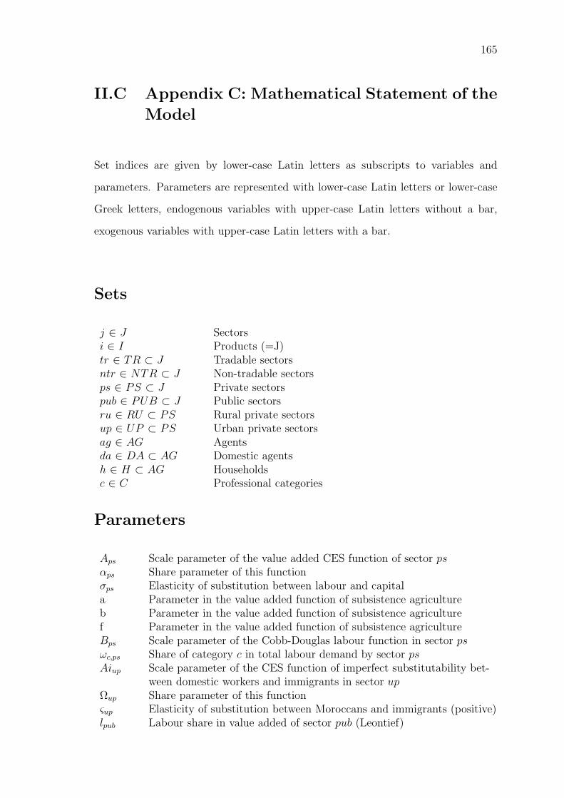
165

II.C Appendix C: Mathematical Statement of the

Model

Set indices are given by lower-case Latin letters as subscripts to variables and

parameters. Parameters are represented with lower-case Latin letters or lower-case

Greek letters, endogenous variables with upper-case Latin letters without a bar,

exogenous variables with upper-case Latin letters with a bar.

Sets

j ∈ J Sectorsi ∈ I Products (=J)tr ∈ TR ⊂ J Tradable sectorsntr ∈ NTR ⊂ J Non-tradable sectorsps ∈ PS ⊂ J Private sectorspub ∈ PUB ⊂ J Public sectorsru ∈ RU ⊂ PS Rural private sectorsup ∈ UP ⊂ PS Urban private sectorsag ∈ AG Agentsda ∈ DA ⊂ AG Domestic agentsh ∈ H ⊂ AG Householdsc ∈ C Professional categories

Parameters

Aps Scale parameter of the value added CES function of sector psαps Share parameter of this functionσps Elasticity of substitution between labour and capitala Parameter in the value added function of subsistence agricultureb Parameter in the value added function of subsistence agriculturef Parameter in the value added function of subsistence agricultureBps Scale parameter of the Cobb-Douglas labour function in sector psωc,ps Share of category c in total labour demand by sector psAiup Scale parameter of the CES function of imperfect substitutability bet-

ween domestic workers and immigrants in sector upΩup Share parameter of this functionςup Elasticity of substitution between Moroccans and immigrants (positive)lpub Labour share in value added of sector pub (Leontief)

166 II. Is International Migration a Cure for Moroccan Unemployment?

kpub Capital share in value added of sector pub (Leontief)lcc,pub Share of category c in total labour demand (Leontief) by public sector pubioj Share of intermediary consumption in the production (Leontief) of sector jvj Share of value added in the production of sector j (Leontief)aiji,j Intermediary consumption of good i by unit of production of sector jtxj Indirect tax rate on product jtmtr Import tariff rate on product trtetr Export tariff rate on product trtyh Direct tax rate on household h’s incometye Direct tax rate on firms’ incomeBrc Scale parameter of the CET function of the rural population of category c$c Share parameter of this functionεc Elasticity of transformation between international rural migrants and nat-

ional workers (negative)Buc Scale parameter of the CET function of the rural population of category c

that decides to stay in Moroccoϑc Share parameter of this function%c Elasticity of transformation between internal migrants and rural workers

(negative)Bic Scale parameter of the CET function of the urban population of category cξc Share parameter of this functionoc Elasticity of transformation between international urban migrants and urban

workers (negative)Betr Scale parameter of the CET production function of sector trδtr Share parameter of this functionκtr Transformation elasticity of the CET production function (negative)ϕtr Price elasticity of export demand of product tr (positive)Amtr Scale parameter of the Armington CES function of product trθtr Share parameter of this functionχtr Substitution elasticity in the Armington function (positive)γi,h Budgetary share of good i in the supernumerary income of household hβc Leisure share in the income of rural household’s member cβ′c Leisure share in the income of urban household’s member clsmaxc Maximal number of working hours offered by rural worker clsmax′c Maximal number of working hours offered by urban worker cλc Share of member c in rural household’s non-labour incomeζ1c Share of internal migrants in labour supply of category cζ2c Share of African immigrants in labour supply of category cλ′c Share of member c in urban household’s non-labour incomeµi Share of product i in total investmentθj Share of the value added of sector j in GDP at factor costψh Household h’s propensity to save

167

ηag Share of capital remuneration received by agent agφag Share of labour remuneration received by agent agDc Scale parameter of the wage curveζ The absolute value of the wage elasticity with respect to unemploymentmc International migration costsimc Internal migration costscs Social security contributionsθ1i Weight of commodity i in the consumer price indexθ2i,“hr” Weight of commodity i in rural consumer price indexθ2i,“hu” Weight of commodity i in urban consumer price index

Endogenous variables

a) Prices

wj Average wage rate of sector jwrc Rural wage rate of professional category cwuc Wage rate of category c in the urban private sectorwgc Wage rate of category c in the urban public sectorwic International wage rate of category c, in foreign currencywnc National wage rate of category cwugc Average urban wage rate of category cwupup Average wage of “warehousemen” in private urban sector upwac Expected urban wage of category crj Capital return in sector jPVj Value added price of sector jPLj Producer price of local product jPDj Market price of local product j sold on the domestic marketPj Production price of sector jPCj Market price of the composite good belonging to sector jPwmtr International import price of product tr, in foreign currencyPwetr International export price of product tr, in foreign currencyPMtr Domestic price of the imported good trPEtr Producer price of the exported good trPfobtr FOB price of the exported good trPINV Aggregate price of investmentPlrc Leisure price of rural household’s member cP luc Leisure price of urban household’s member ce Nominal exchange rate (the price of a unit of foreign currency in

domestic currency)CPI Consumer price indexCPIR Consumer price index in rural areasCPIU Consumer price index in urban areasPindex GDP deflator, numeraire

168 II. Is International Migration a Cure for Moroccan Unemployment?

b) Production

XSj Production of sector j (volume)V Aj Value added of sector j (volume)DIi,j Intermediary demand of product i by sector j (volume)CIj Total intermediary consumption of sector j (volume)

c) Factors of production

KDj Capital demand by sector j (volume)LDRru Labour demand by rural sector ru (volume)LRc,ru Labour demand of category c by rural sector ru (volume)LDUup Labour demand by urban private sector up (volume)LUc,up Labour demand of category c by urban private sector up (volume)LDGpub Labour demand by public sector pub (volume)LGc,pub Labour demand of category c by urban public sector pub (volume)LSRc Rural population belonging to category cLSUc Urban population belonging to category cuc Urban unemployment rate of category c

d) Migration

NATc Rural workers of category c who decide to stay in MoroccoEMRc Rural emigrant flow of category cNATRc Rural workers of category c who decide to stay in rural areasMIGc Rural migrant flow of category c to urban areasNATUc Urban workers of category c who decide to stay in urban areasEMUc Urban emigrant flow of category cIMMIGcThe stock of Sub-Saharan immigrants belonging to category cNATIup The demand of national “warehousemen” by urban private sector upETRup The demand of Sub-Saharan “warehousemen” by urban private sector up

e) Income/Savings

Yag Agent ag’s incomeY Dh Disposable income of household hSag Agent ag’s savingsTag,ag Transfers between agents

f) Tax revenues

TIj Indirect taxes on product jTIMtr Import tariffs on product trTIEtr Export tariffs on product tradj Compensatory tax

169

g) External trade

EXStr Export supply of product tr (volume)DOMj Domestic production of sector j sold on the domestic market (volume)Qj Supply of the composite product belonging to sector j (volume)EXDtr Export demand of product tr (volume)Mtr Import demand of product tr (volume)

h) Final demand

CTi,h Consumption of good i by household h (volume)Cmini,h Minimum consumption of good i by household h (volume)BCh Consumption budget of household hIBCc,h Consumption budget of member c belonging to household hGi Public consumption of product i (volume)DITi Total intermediary consumption of product i (volume)INVi Investment demand of product i (volume)STKi Stock variation of product i (volume)ITV OL Gross fixed capital formation (volume)IT Gross fixed capital formation (value)

Exogenous variables

wgc Wage rate of category c in the urban public sectorwic International wage rate of category c, in foreign currencyrpub Capital return of public sector pubKDps Capital demand by sector psPwmtr International import price of product tr, in foreign currencyPwetr International export price of product tr, in foreign currencyIMMIGcThe stock of Sub-Saharan immigrants belonging to category cCmini,h Minimum consumption of product i by household hGi Public consumption of product iSTKi Stock variation of product iITV OL Gross fixed capital formation (volume)S“row” External savingsTh,da Transfers by agent da to household hT“fm”,da Transfers by agent da to firmsT“row”,da Transfers by agent da to the RoW, in foreign currencyT“gv”,“gv” Transfers made by the government to itselfTag,“row” Transfers by the RoW to agent ag, in foreign currencyPindex GDP deflator, numeraire

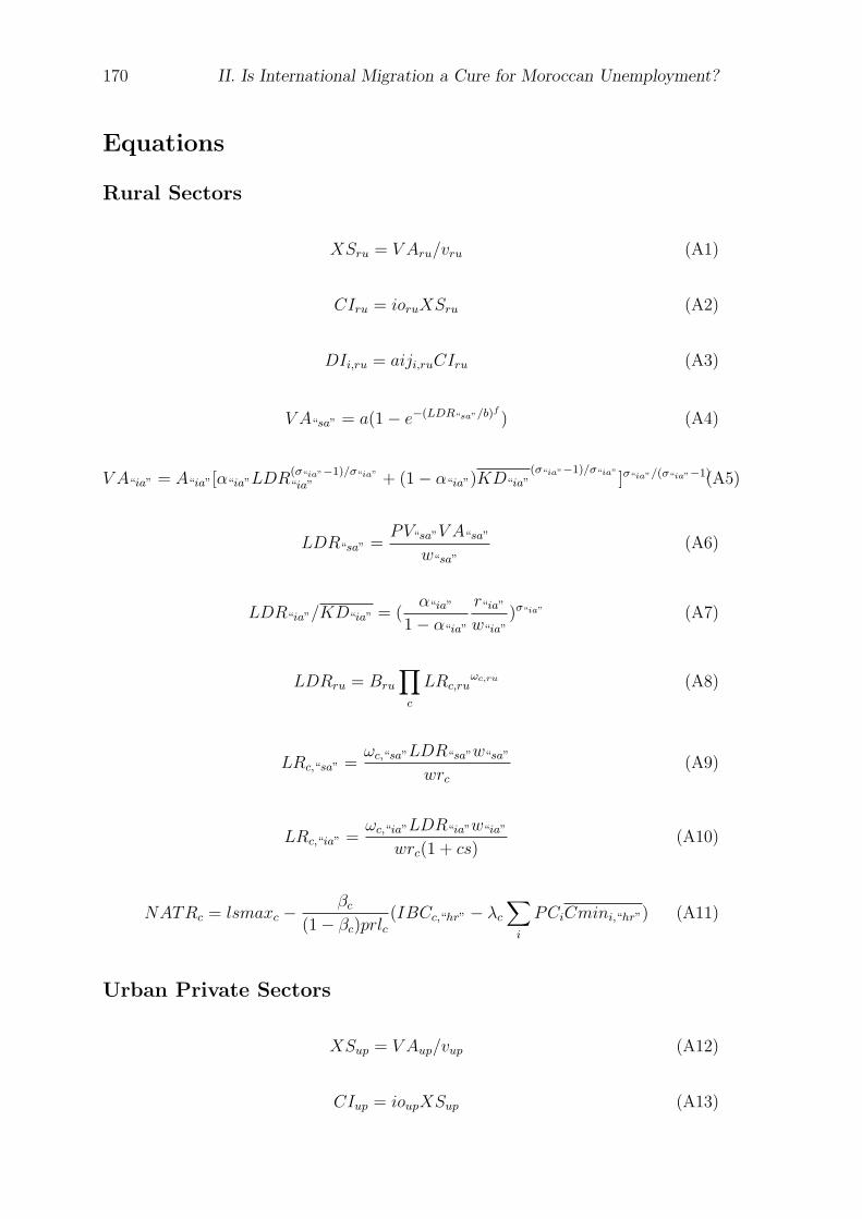
170 II. Is International Migration a Cure for Moroccan Unemployment?

Equations

Rural Sectors

XSru = V Aru/vru (A1)

CIru = ioruXSru (A2)

DIi,ru = aiji,ruCIru (A3)

V A“sa” = a(1− e−(LDR“sa”/b)f

) (A4)

V A“ia” = A“ia”[α“ia”LDR(σ“ia”−1)/σ“ia”

“ia” + (1− α“ia”)KD“ia”(σ“ia”−1)/σ“ia”

]σ“ia”/(σ“ia”−1)(A5)

LDR“sa” =PV“sa”V A“sa”

w“sa”

(A6)

LDR“ia”/KD“ia” = (α“ia”

1− α“ia”

r“ia”

w“ia”

)σ“ia” (A7)

LDRru = Bru

∏c

LRc,ruωc,ru (A8)

LRc,“sa” =ωc,“sa”LDR“sa”w“sa”

wrc(A9)

LRc,“ia” =ωc,“ia”LDR“ia”w“ia”

wrc(1 + cs)(A10)

NATRc = lsmaxc −βc

(1− βc)prlc(IBCc,“hr” − λc

∑i

PCiCmini,“hr”) (A11)

Urban Private Sectors

XSup = V Aup/vup (A12)

CIup = ioupXSup (A13)

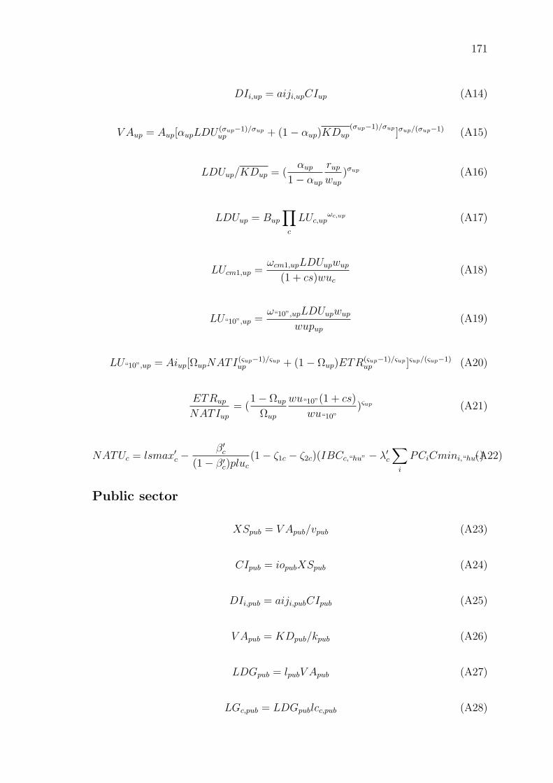
171

DIi,up = aiji,upCIup (A14)

V Aup = Aup[αupLDU(σup−1)/σupup + (1− αup)KDup

(σup−1)/σup]σup/(σup−1) (A15)

LDUup/KDup = (αup

1− αuprupwup

)σup (A16)

LDUup = Bup

∏c

LUc,upωc,up (A17)

LUcm1,up =ωcm1,upLDUupwup

(1 + cs)wuc(A18)

LU“10”,up =ω“10”,upLDUupwup

wupup(A19)

LU“10”,up = Aiup[ΩupNATI(ςup−1)/ςupup + (1− Ωup)ETR

(ςup−1)/ςupup ]ςup/(ςup−1) (A20)

ETRup

NATIup= (

1− Ωup

Ωup

wu“10”(1 + cs)

wu“10”

)ςup (A21)

NATUc = lsmax′c −β′c

(1− β′c)pluc(1− ζ1c − ζ2c)(IBCc,“hu” − λ′c

∑i

PCiCmini,“hu”)(A22)

Public sector

XSpub = V Apub/vpub (A23)

CIpub = iopubXSpub (A24)

DIi,pub = aiji,pubCIpub (A25)

V Apub = KDpub/kpub (A26)

LDGpub = lpubV Apub (A27)

LGc,pub = LDGpublcc,pub (A28)

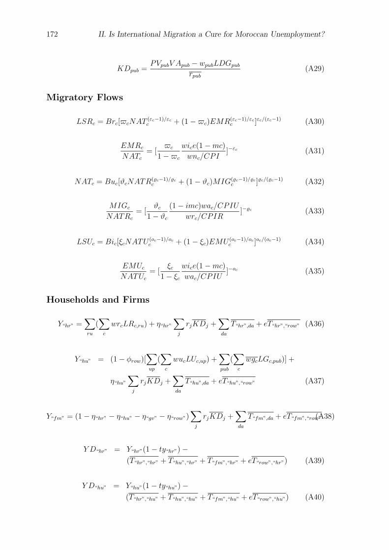
172 II. Is International Migration a Cure for Moroccan Unemployment?

KDpub =PVpubV Apub − wpubLDGpub

rpub(A29)

Migratory Flows

LSRc = Brc[$cNAT(εc−1)/εcc + (1−$c)EMR(εc−1)/εc

c ]εc/(εc−1) (A30)

EMRc

NATc= [

$c

1−$c

wice(1−mc)wnc/CPI

]−εc (A31)

NATc = Buc[ϑcNATR(%c−1)/%cc + (1− ϑc)MIG(%c−1)/%c

c ]%c/(%c−1) (A32)

MIGc

NATRc

= [ϑc

1− ϑc(1− imc)wac/CPIU

wrc/CPIR]−%c (A33)

LSUc = Bic[ξcNATU(oc−1)/occ + (1− ξc)EMU (oc−1)/oc

c ]oc/(oc−1) (A34)

EMUcNATUc

= [ξc

1− ξcwice(1−mc)wac/CPIU

]−oc (A35)

Households and Firms

Y“hr” =∑ru

(∑c

wrcLRc,ru) + η“hr”

∑j

rjKDj +∑da

T“hr”,da + eT“hr”,“row” (A36)

Y“hu” = (1− φrow)[∑up

(∑c

wucLUc,up) +∑pub

(∑c

wgcLGc,pub)] +

η“hu”

∑j

rjKDj +∑da

T“hu”,da + eT“hu”,“row” (A37)

Y“fm” = (1− η“hr” − η“hu” − η“gv” − η“row”)∑j

rjKDj +∑da

T“fm”,da + eT“fm”,“row”(A38)

Y D“hr” = Y“hr”(1− ty“hr”)−(T“hr”,“hr” + T“hu”,“hr” + T“fm”,“hr” + eT“row”,“hr”) (A39)

Y D“hu” = Y“hu”(1− ty“hu”)−(T“hr”,“hu” + T“hu”,“hu” + T“fm”,“hu” + eT“row”,“hu”) (A40)

173

Sh = ψhY Dh (A41)

BCh = Y Dh − Sh (A42)

S“fm” = Y“fm” −∑da

Tda,“fm” − eT“row”,“fm” (A43)

The Government

TItr = txtradj(PtrXStr − PEtrEXStr) + txtradj(1 + tmtr)ePmwtrMtr (A44)

TIntr = txntradjPLntrXSntr (A45)

TIMtr = tmtrePwmtrMtr (A46)

TIEtr = tetrPEtrEXStr (A47)

T“gv”,h = tyhYh (A48)

T“gv”,“fm” = tyeY“fm” (A49)

Y“gv” = η“gv”

∑j

rjKDj +∑tr

TIMtr +∑tr

TIEtr +∑j

TIj +∑da

T “gv”,da +

eT“gv”,“rw” + (∑up

wupLDUup −∑up

(∑c

wucLUc,up)) +

(w“ar”LDR“ar” −∑c

wrcLRc,“ar”)) (A50)

S“gv” = Y“gv” −∑i

PCiGi −∑da

Tda,“gv” − eT“row”,“gv” (A51)

External Trade

XStr = Betr[δtrEXS(κtr−1)/κtrtr + (1− δtr)DOM (κtr−1)/κtr

tr ]κtr/(κtr−1) (A52)

XSntr = DOMntr (A53)

174 II. Is International Migration a Cure for Moroccan Unemployment?

EXStrDOMtr

= (δtr

1− δtrPLtrPEtr

)κtr (A54)

EXDtr = EXDOtr(PwetrPfobtr

)ϕtr (A55)

Qtr = Amtr[θtrM(χtr−1)/χtrtr + (1− θtr)DOM (χtr−1)/χtr

tr ]χtr/(χtr−1) (A56)

Qntr = DOMntr (A57)

Mtr

DOMtr

= (θtr

1− θtrPDtr

PMtr

)χtr (A58)

S“row” =∑tr

PwmtrMtr + η“row”

∑j rjKDj

e+

∑ag

T“row”,ag +

φrow

∑up(

∑cwucLUc,up) +

∑pub(

∑cwgcLGc,pub)

e− (A59)∑

tr

PfobtrEXStr −∑ag

Tag,row

Final Demand

CTi,“hr” = Cmini,“hr” +γi,“hr”PCi

(BC“hr” −∑i

PCiCmini,“hr”) (A60)

CTi,“hu” = Cmini,“hu” +γi,“hu”

PCi(BC“hu” −

∑i

PCiCmini,“hu”) (A61)

IBCc,“hr” = (1− ψ“hr”)(1− ty“hr”)wrc∑ru

LRc,ru + (A62)

λc(1− ψ“hr”)(1− ty“hr”)[Y“hr” −∑c

(wrc∑ru

LRc,ru)]

IBCc,“hu” = (1− ψ“hu”)(1− ty“hu”)(wuc∑up

LUc,up + wgc∑pub

LGc,pub) (A63)

+λ′c(1− ψ“hu”)(1− ty“hu”)[Y“hu” −∑c

(wuc∑up

LUc,up + wgc∑pub

LGc,pub)]

INVi = µiIT/PCi (A64)

175

DITi =∑i

aiji,jCIj (A65)

Prices

lnwucCPIU

= Dc − ζ lnuc (A66)

wgc wuc (A67)

wnc =wrc

∑ru LRc,ru + wuc

∑up LUc,up + wgc

∑pub LGc,pub∑

ru LRc,ru +∑

up LUc,up +∑

pub LGc,pub

(A68)

wugc =wuc

∑up LUc,up + wgc

∑pub LGc,pub∑

up LUc,up +∑

pub LGc,pub

(A69)

wpub =∑c

wgcLGc,pub

LDGpub

(A70)

wac = wugc

∑up LUc,up +

∑pub LGc,pub

NATUc + (1− imc)MIGc + IMMIGc

(A71)

wupup =(1 + cs)wu“10”NATIup + wu“10”ETRup

LU“10”,up

(A72)

r“ia” =PV“ia”V A“ia” − w“ia”LDR“ia”

KD“ia”

(A73)

rup =PVupV Aup − wupLDUup

KDup

(A74)

PVj =PjXSj −

∑i PCiDIi,j

V Aj(A75)

PMtr = ePwmtr(1 + tmtr)(1 + txtradj) (A76)

PEtr =ePfobtr

(1 + tetr)(A77)

176 II. Is International Migration a Cure for Moroccan Unemployment?

PCtr =DOMtrPDtr +MtrPMtr

Qtr

(A78)

PCntr = PDntr (A79)

PDj = PLj(1 + txjadj) (A80)

Ptr =PLtrDOMtr + PEtrEXStr

XStr(A81)

Pntr = PLntr (A82)

PINV =∏i

(PCiµi

)µi

(A83)

Plrc = (1− ψ“hr”)(1− ty“hr”)wrc (A84)

Pluc = (1− ψ“hu”)(1− ty“hu”)(1− uc)wugc (A85)

CPI =∑i

θ1iPCi (A86)

CPIR =∑i

θ2i,“hr”PCi (A87)

CPIU =∑i

θ2i,“hu”PCi (A88)

Pindex =∑j

θjPVj (A89)

Equilibrium Conditions and Closure

NATRc =∑ru

LRc,ru (A90)

(NATUc + (1− imc)MIGc + IMMIGc)(1− uc) =∑up

LUc,up +∑pub

LGc,pub(A91)

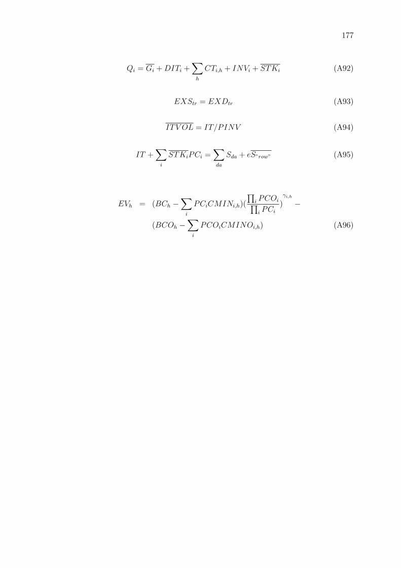
177

Qi = Gi +DITi +∑h

CTi,h + INVi + STKi (A92)

EXStr = EXDtr (A93)

ITV OL = IT/PINV (A94)

IT +∑i

STKiPCi =∑da

Sda + eS”row” (A95)

EVh = (BCh −∑i

PCiCMINi,h)(

∏i PCOi∏i PCi

)γi,h

−

(BCOh −∑i

PCOiCMINOi,h) (A96)

178 II. Is International Migration a Cure for Moroccan Unemployment?

II.D Appendix D: Sensitivity Analysis

Table II.11: Unemployment For Selected Values of Wage Elasticity ζPercentage Change with Respect to the Base Year with Shock SIM3Categories ζ = 0.05 ζ = 0.2 ζ = 0.3 ζ = 0.4 ζ = 0.5Directors 0.23 0.11 0.08 0.06 0.05Senior executive -0.05 -0.10 -0.09 -0.08 -0.07Junior staff 0.12 0.07 0.05 0.04 0.03Employees 0.05 0.02 0.01 0.01 0.01Commercants -0.23 -0.18 -0.14 -0.12 -0.10Farmers 16.98 4.32 2.88 2.16 1.73Craftsmen 0.18 0.11 0.08 0.07 0.06Farm labourers 15.11 4.74 3.24 2.46 1.98Drivers 0.17 0.10 0.08 0.06 0.05Warehousemen 0.98 0.64 0.51 0.43 0.37

Notes: ζ: The absolute value of the wage elasticity with respect to unemployment.Source: Author’s calculations.

Table II.12: Unemployment For Selected Combinationsof Rural and Urban Income Elasticities of Labour Supply

Percentage Change with Respect to the Base Year with Shock SIM3Rural Urban Senior JuniorElasticity Elasticity Directors Executive Staff Employees Commercants-0.1 -0.1 0.17 -0.09 0.10 0.04 -0.22-0.1 -0.2 0.17 -0.09 0.10 0.04 -0.22-0.1 -0.4 0.17 -0.09 0.10 0.04 -0.22-0.2 -0.1 0.17 -0.09 0.10 0.04 -0.22-0.2 -0.2 0.17 -0.09 0.10 0.04 -0.22-0.2 -0.4 0.17 -0.09 0.10 0.04 -0.22-0.4 -0.1 0.17 -0.09 0.10 0.04 -0.22-0.4 -0.2 0.17 -0.09 0.10 0.04 -0.22-0.4 -0.4 0.17 -0.09 0.10 0.04 -0.22

Source: Author’s calculations.

Rural Urban FarmElasticity Elasticity Farmers Craftsmen Labourers Drivers Warehousemen-0.1 -0.1 8.60 0.15 8.77 0.14 0.83-0.1 -0.2 8.60 0.15 8.77 0.14 0.83-0.1 -0.4 8.60 0.15 8.77 0.14 0.83-0.2 -0.1 8.60 0.15 8.77 0.14 0.83-0.2 -0.2 8.60 0.15 8.77 0.14 0.83-0.2 -0.4 8.60 0.15 8.77 0.14 0.83-0.4 -0.1 8.60 0.15 8.77 0.14 0.83-0.4 -0.2 8.60 0.15 8.77 0.14 0.83-0.4 -0.4 8.60 0.15 8.77 0.14 0.83

Table II.13: Unemployment For Selected Combinationsof Migration Elasticities

Percentage Change with Respect to the Base Year with Shock SIM3Senior Junior

ε % o Directors Executive Staff Employees Commercants-0.75 -1.25 -1 0.13 -0.09 0.08 0.02 -0.22-0.75 -1.25 -2 0.13 -0.09 0.08 0.02 -0.22-0.75 -1.25 -4 0.13 -0.09 0.08 0.02 -0.22-0.75 -2.5 -1 0.17 -0.09 0.10 0.04 -0.22-0.75 -2.5 -2 0.17 -0.09 0.10 0.04 -0.22-0.75 -2.5 -4 0.17 -0.09 0.10 0.04 -0.22-0.75 -5 -1 0.23 -0.11 0.12 0.07 -0.26-0.75 -5 -2 0.23 -0.11 0.12 0.07 -0.26-0.75 -5 -4 0.23 -0.11 0.12 0.07 -0.26-1.5 -1.25 -1 0.13 -0.09 0.08 0.02 -0.22-1.5 -1.25 -2 0.13 -0.09 0.08 0.02 -0.22-1.5 -1.25 -4 0.13 -0.09 0.08 0.02 -0.22-1.5 -2.5 -1 0.17 -0.09 0.10 0.04 -0.22-1.5 -2.5 -2 0.17 -0.09 0.10 0.04 -0.22-1.5 -2.5 -4 0.17 -0.09 0.10 0.04 -0.22-1.5 -5 -1 0.23 -0.11 0.12 0.07 -0.26-1.5 -5 -2 0.23 -0.11 0.12 0.07 -0.26-1.5 -5 -4 0.23 -0.11 0.12 0.07 -0.26-3 -1.25 -1 0.13 -0.09 0.08 0.02 -0.22-3 -1.25 -2 0.13 -0.09 0.08 0.02 -0.22-3 -1.25 -4 0.13 -0.09 0.08 0.02 -0.22-3 -2.5 -1 0.17 -0.09 0.10 0.04 -0.22-3 -2.5 -2 0.17 -0.09 0.10 0.04 -0.22-3 -2.5 -4 0.17 -0.09 0.10 0.04 -0.22-3 -5 -1 0.23 -0.11 0.12 0.07 -0.26-3 -5 -2 0.23 -0.11 0.12 0.07 -0.26-3 -5 -4 0.23 -0.11 0.12 0.07 -0.26Notes: (1)εc: Elasticity of transformation between international rural migrants and national workers.(2)%c: Elasticity of transformation between internal migrants and rural workers.(3)oc: Elasticity of transformation between international urban migrants and urban workers.Source: Author’s calculations.

Farmε % o Farmers Craftsmen Labourers Drivers Warehousemen-0.75 -1.25 -1 7.88 0.13 8.62 0.10 0.76-0.75 -1.25 -2 7.88 0.13 8.62 0.10 0.76-0.75 -1.25 -4 7.88 0.13 8.62 0.10 0.76-0.75 -2.5 -1 8.60 0.15 8.77 0.14 0.83-0.75 -2.5 -2 8.60 0.15 8.77 0.14 0.83-0.75 -2.5 -4 8.60 0.15 8.77 0.14 0.83-0.75 -5 -1 9.24 0.19 8.83 0.21 0.97-0.75 -5 -2 9.24 0.19 8.83 0.21 0.97-0.75 -5 -4 9.24 0.19 8.83 0.21 0.97-1.5 -1.25 -1 7.88 0.13 8.62 0.10 0.76-1.5 -1.25 -2 7.88 0.13 8.62 0.10 0.76-1.5 -1.25 -4 7.88 0.13 8.62 0.10 0.76-1.5 -2.5 -1 8.60 0.15 8.77 0.14 0.83-1.5 -2.5 -2 8.60 0.15 8.77 0.14 0.83-1.5 -2.5 -4 8.60 0.15 8.77 0.14 0.83-1.5 -5 -1 9.24 0.19 8.83 0.21 0.97-1.5 -5 -2 9.24 0.19 8.83 0.21 0.97-1.5 -5 -4 9.24 0.19 8.83 0.21 0.97-3 -1.25 -1 7.88 0.13 8.62 0.10 0.76-3 -1.25 -2 7.88 0.13 8.62 0.10 0.76-3 -1.25 -4 7.88 0.13 8.62 0.10 0.76-3 -2.5 -1 8.60 0.15 8.77 0.14 0.83-3 -2.5 -2 8.60 0.15 8.77 0.14 0.83-3 -2.5 -4 8.60 0.15 8.77 0.14 0.83-3 -5 -1 9.24 0.19 8.83 0.21 0.97-3 -5 -2 9.24 0.19 8.83 0.21 0.97-3 -5 -4 9.24 0.19 8.83 0.21 0.97

Chapter III

When Migrant Remittances Are

Not Everlasting, How Can

Morocco Make Up?

The static CGE model built in Chapter 2 helped determine the direct impact of

migration on Moroccan labour market. Nevertheless, migration has as well indirect

effects on the sending economy through remittances. This indirect effect was not

taken into account in Chapter 2 so that the results would be comparable with those

of the literature on the subject. It is however investigated in the present chapter.

According to data from the IMF’s Balance of Payments Yearbook, Morocco is the

fourth-largest recipient of official remittances among developing countries, totalling

USD 3.3 billion (MAD 37 billion) in 2001. After their surge in 2001, their level

remained high compared to other developing countries, about 9% of GDP and 25%

of exports. For instance, they amounted to only 3% of GDP and 16% of exports in

Egypt, 1% of GDP and 3% of exports in Turkey, 5% of GDP and 13% of exports in

Tunisia (Bouhga-Hagbe, 2004). Since the early 70s, they have become increasingly

0 This chapter is based on Karam (2008).

181

182 III. When Migrant Remittances Are Not Everlasting, How Can Morocco Make Up?

important for the Moroccan BoP. In 2001, they were six times higher than ODA

and five times higher than FDI (de Haas, 2007). They represent the country’s major

source of foreign currency receipts and exceed receipts from phosphate and tourism

(Nyberg-Sorensen, 2004).

Unlike the best part of the literature that focuses on households, ignoring linkages

that transmit the influence of migration and remittances to other households and

economic sectors, I use a CGE approach to investigate the impact of remittances

on Morocco. To take into account the use of remittances for investment needs, I

adopt a dynamic framework that allows the allocation of investment to the different

sectors. I further assume a segmentation of the savings market in order to show

clearly that remittances, unlike other sources of savings, mainly finance investment

in real estate.

The scale and growth of remittances by destination of developing countries

have attracted increased attention regarding their development impact. Many

studies were concerned by their effect on poverty and inequality, on the balance

of payments, and others by their use for consumption and investment needs.

Putting aside the poverty reducing effect of remittances on which the different

studies agree (Adams, 2006; Yang and Martinez, 2006), the results are mixed.

To begin with, empirical works on the income distribution effects of remittances

are not conclusive1. Secondly, remittances are supposed to affect unemployment,

productivity and growth, depending on the breakdown between consumption and

investment. If they are invested, they will promote output and employment and

thereby finance future consumption in a sustainable way. Alternatively, if they

are spent only on current consumption goods, then future consumption has to be

1 For example, Ahlburg (1996) and Taylor and Wyatt (1996) find that remittances have anequalising effect on income distribution in Tonga and Mexico. By contrast, evidence fromEgypt (Adams, 1991), Pakistan (Adams, 1998) and the Philippines (Rodriguez, 1998) showthat remittances induced income inequality to rise. Adams (2006) shows that internal andinternational remittances have little impact on income inequality in Guatemala. The evidencefrom the Mexican case found support to the inverse U-shape relationship between migration andinequality (McKenzie and Rapoport, 2005).

183

financed by future remittances. However, Glytsos (1993) argues that remittances,

even when not invested, can have an important multiplier effect. His study applied

to Greece shows that this multiplier effect arises when consumption stimulates the

demand of goods and services, which promotes, in turn, output and employment.

Third, remittances affect the BoP and they have a more positive impact than

other monetary flows such as financial aid, FDI and loans because they are a more

stable source of foreign currency, bear no interest and do not have to be repaid.

But one should be cautious here because remittance flows can also have negative

inflationary effects if they stimulate demand more than supply and this demand

falls on non-tradable goods. Finally, they can induce a moral hazard problem where

people choose to work less due to the positive income effect of remittances (Chami,

Fullenkamp and Jahjah, 2005).

The results of the previous works show that the effects of remittances are

heterogeneous across space and depend on the amount of remittances received

and other macroeconomic variables that are country-specific. In this context, it is

worth mentioning that the literature is unevenly distributed with regard to country

analyses. A lot of works have been done on Latin migrants living in the US while

the interest for migrants from MENA countries in the EU has just begun, in spite of

the large flows of remittances received by these countries. According to the IMF’s

Balance of Payments Yearbook, MENA countries received in 2001, as well as South

Asia, the largest flow of remittances in percentage of GDP (2.3%) and the second

largest flow, after Latin America and the Caribbean, in billions of US dollars (USD

14 billion v/s USD 23 billion). In particular, Morocco is ranked first between MENA

countries and stood internationally after India, Mexico and the Philippines in 2001.

Despite its place among the largest developing countries receiving remittances, works

concerned by the impact of remittances on Morocco are limited to unpublished

reports, theses or working papers on particular regions2. On the national level,

only general surveys like those of Hamdouch (2000) and Nyberg-Sorensen (2004)

2 See for example Berriane (1996), Lazaar (1987, 1989), McMurray (1992) cited in Nyberg-Sorensen(2004) on the Rif Mountains, and Bijaad (1987), de Haas (2003, 2006) on Southern Morocco.

184 III. When Migrant Remittances Are Not Everlasting, How Can Morocco Make Up?

are available. Regardless of empirical gaps and methodological flaws, available

evidence suggests that migration and remittances have considerably improved living

conditions, education, and triggered economic activity, from which non-migrants

have indirectly profited. However, this impact is fundamentally heterogeneous

across space and time, as well as across socio-ethnic and gender groups. In many

cases, the development of migrant-sending regions is a prerequisite for return and/or

investment rather than a consequence of migration. Consequently, additional works

are needed to assess the effects of migration on marginal propensities to invest and

multiplier effects of remittance expenditure (de Haas, 2007).

Yet, the literature based on households or on CGE models3 has given less

attention to the sectoral distribution of remittances invested, especially when the

largest part of remittances in developing countries is invested in real estate. The

problem with this sector is that construction services are offered domestically, unlike

other sectors that export to international markets and compete with international

products. On the one hand, increasing openness generates strong competitive

pressures that drive costs down and ameliorate the product quality. On the

other hand, it accelerates institutional change that reduces transaction costs for

all business activities. This is the export-growth relationship in the heart of export-

led growth strategy. In order to model the particular investment of remittances

in real estate in a dynamic CGE framework, I resort to a segmentation of the

savings market: unlike FDI and domestic savings that finance productive sectors,

remittances finance mainly the real estate sector. Indeed, remittances by Moroccans

residing abroad (MRA) are driven by altruistic motives: they tend to satisfy the

family basic needs, among other things having more comfortable and decent houses.

If remittances are treated analogously to foreign and domestic savings that finance

productive sectors, this will overestimate the volume of capital invested in these

sectors and create an illusion of a sustainable growth. This is the main contribution

of this chapter. Then, I look to the long-term tendency of migratory flows and

3 I could identify only few CGE models studying the impact of remittances in a dynamic framework.See for example the paper of Taylor and Dyer (2006) on Mexico.

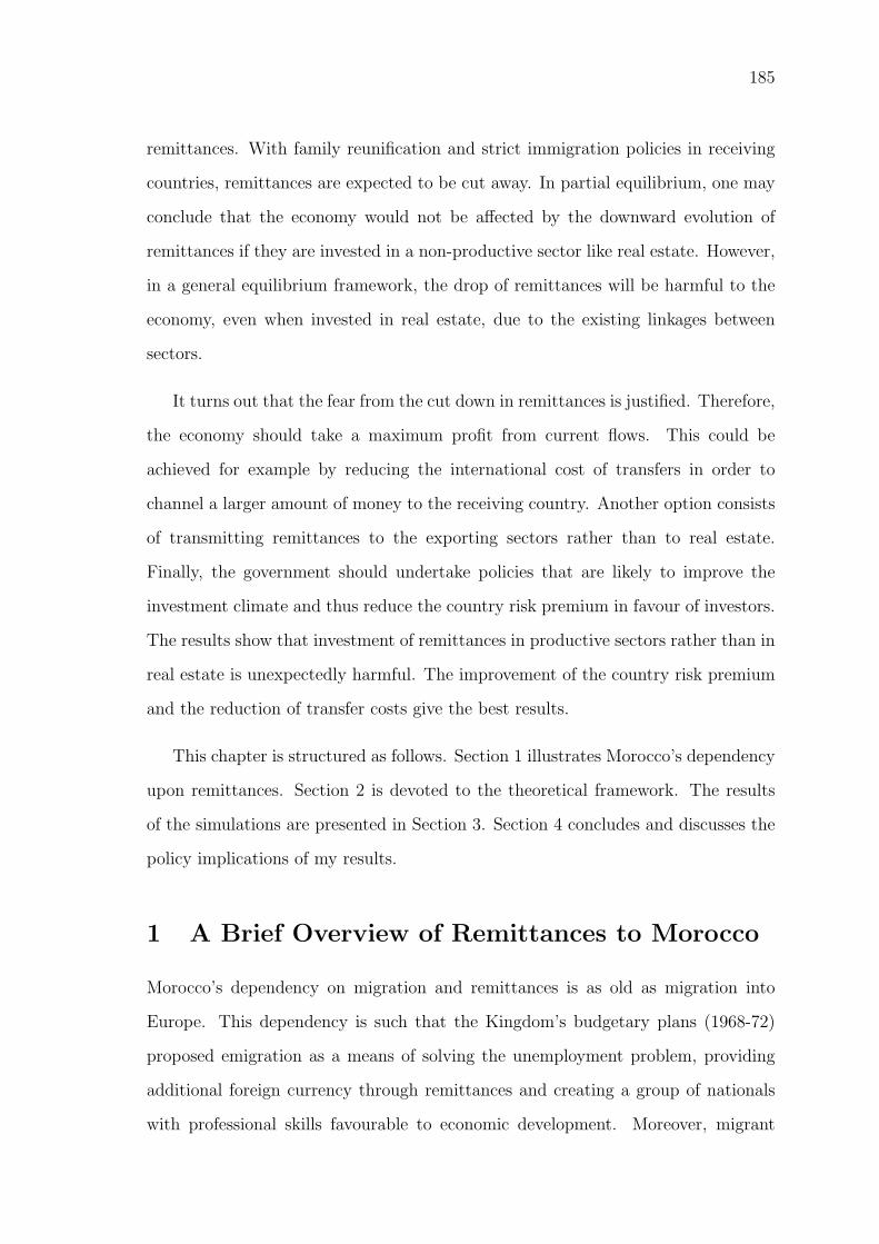
185

remittances. With family reunification and strict immigration policies in receiving

countries, remittances are expected to be cut away. In partial equilibrium, one may

conclude that the economy would not be affected by the downward evolution of

remittances if they are invested in a non-productive sector like real estate. However,

in a general equilibrium framework, the drop of remittances will be harmful to the

economy, even when invested in real estate, due to the existing linkages between

sectors.

It turns out that the fear from the cut down in remittances is justified. Therefore,

the economy should take a maximum profit from current flows. This could be

achieved for example by reducing the international cost of transfers in order to

channel a larger amount of money to the receiving country. Another option consists

of transmitting remittances to the exporting sectors rather than to real estate.

Finally, the government should undertake policies that are likely to improve the

investment climate and thus reduce the country risk premium in favour of investors.

The results show that investment of remittances in productive sectors rather than in

real estate is unexpectedly harmful. The improvement of the country risk premium

and the reduction of transfer costs give the best results.

This chapter is structured as follows. Section 1 illustrates Morocco’s dependency

upon remittances. Section 2 is devoted to the theoretical framework. The results

of the simulations are presented in Section 3. Section 4 concludes and discusses the

policy implications of my results.

1 A Brief Overview of Remittances to Morocco

Morocco’s dependency on migration and remittances is as old as migration into

Europe. This dependency is such that the Kingdom’s budgetary plans (1968-72)

proposed emigration as a means of solving the unemployment problem, providing

additional foreign currency through remittances and creating a group of nationals

with professional skills favourable to economic development. Moreover, migrant

186 III. When Migrant Remittances Are Not Everlasting, How Can Morocco Make Up?

remittances would help finance internal investments. The five-year plan of 1973-77

further proposed to set up a network of social bureaus abroad.

Morocco is the fourth-largest developing country receiving official remittances,

totalling MAD 37 billion (USD 3.3 billion) in 2001. Remittance flows moved from

MAD 2 billion in 1975 to MAD 10 billion in 1985 and MAD 19 billion in 1998. They

reached a record level of nearly MAD 37 billion in 2001 before moving down to MAD

32 billion in 2002. In 2003, they rose again to MAD 35 billion. They have particularly

increased during the past five years, encouraged by some events such as the renewed

interest of the new king for the Moroccan community living abroad, the adoption

of the Euro that dismantled the savings made in the old European currencies, the

devaluation of the Dirham in 2001, the strong increase in the number of Moroccan

immigrants to Italy and Spain and the remarkable attachment of Moroccans to

their country of origin. Remittances role in the BoP is often higher than phosphate,

tourism, foreign investments and private loans (Figure III.1).

Figure III.1:Remittances and other flows of the BoP, 1998-2007 (MAD million)

0

10000

20000

30000

40000

50000

60000

70000

1998 1999 2000 2001 2002 2003 2004 2005 2006 2007

Phosphate Exports Remittances Tourism Foreign Investments and Private Loans

Notes: The word remittances refers here to workers’ remittances that are registered as currenttransfers.Source: Ministry of Foreign Trade, Rabat.

187

As it is shown in Figure III.2, remittances almost cover the trade deficit and have

contributed to the recent surpluses of the external current account, as well as the

overall BoP surplus. In spite of their magnitude in the balance of payments, they do

not seem to constitute a significant risk in terms of stability because they are mainly

driven by altruism and attachment to the home country. Portfolio diversification

motives are not significant among the long run explanatory factors of remittances

to Morocco (Bouhga-Hagbe, 2004). According to van Dalen et al. (2005), it is the

parent-child relation that determines the motive for remitting money.

Figure III.2:Remittances as % of trade deficit, 1998-2007 (Values in MAD million)

-150000

-100000

-50000

0

50000

100000

1998 1999 2000 2001 2002 2003 2004 2005 2006 2007

Remittances Trade Deficit

64% 59% 53%84% 72% 66% 53% 48% 49%

41%

Notes: The word remittances refers here to workers’ remittances that are registered as currenttransfers.Source: Ministry of Foreign Trade, Rabat.

However, the long term tendency goes against the increase of remittances.

With the restriction of Western immigration policies, the rise in the number of

educated migrants that tend to settle abroad, family reunification, naturalisation,

and the succession of generations living abroad, remittances are expected to decrease,

negatively affecting the Moroccan economy largely dependent on this source of

foreign currency. That is why it is important to know the treatment reserved for

188 III. When Migrant Remittances Are Not Everlasting, How Can Morocco Make Up?

them: are they consumed or invested? And if invested, are they in productive

sectors? In this context, the allocation of remittances between sectors plays an

essential role, mainly because the best part is invested in real estate. First,

construction services are offered domestically and do not profit from technical

progress due to competitiveness with international products. Secondly, real estate

only accounts for 4% of GDP at factor costs, compared to 17% for agriculture, 14%

for trade and repair and 11% for rental services. Besides, it only constitutes 3%

of the wage payroll compared to 34% in agriculture. At first sight, one concludes

that remittances should be channelled to productive sectors in order to promote the

economic activity and guarantee the conditions of a sustainable growth.

The main purpose of sending money to Morocco is to support the family and

other close relatives and/or build a house. Real estate monopolizes the lion’s share

with nearly 83.7% of investments by MRA in their country of origin. There is only

limited evidence of investments in productive sectors (Table III.1). Migrants find

it difficult and unattractive to make investments in Morocco because of the lack of

information about investment opportunities, a slow bureaucratic system, widespread

corruption and the insecurity resulting from the economic and political situation. To

this is added, especially in rural villages, the lack of infrastructure such as electricity,

water and roads that deeply inhibits the productive use of remittances.

However, things are changing: first, fewer migrants consider investing in the

future. Secondly, future projects are more concentrated into productive sectors

(Table III.1). Real estate, while remaining the principal sector of investment,

consists of no more than 35.6% of the projects. This reflects the change in migrants’

behaviour, especially the second generation of migrants, and also the fact that MRA

have already invested heavily in real estate.

Transfers are increasingly taking place through official channels after the tighter

control imposed by the authorities on financial flows to and from Arab countries in

the wave of the “war on terror” declared by the United Nations (FEMISE, 2004).

Official remittance flows have also been stimulated by the expansion of the national

189

Table III.1: Sectoral distribution of MRA’s investments (%)Sectors MRA’s investments MRA’s investment

projectsReal estate 83.7 35.6Agriculture 7.5 10.6Trade 4.9 27.4Tourism 1.4 12.1Manufacturing 1.3 7.5Other services 1.1 5.3Other sectors 0.1 1.5

Source: Hamdouch (2000).

banking system and the extension of banking services to the principal immigration

countries. More than 62% of migrants transfer their funds through Moroccan banks4

compared with only 4.4% for foreign banks. 16% of migrants use the post office and

3.4% private intermediaries (Hamdouch, 2000). The Banque Populaire charges low

commission for money transfer (the half of that charged by private companies).

However, according to Hamdouch (2000), transfer costs should be further reduced

and transfer delays shortened. Table III.2 presents an example of transfer costs

charged by different channels from the Netherlands to Morocco. Moreover, the

major problem is the lack of transparency on the cost and speed of the transaction:

product information can only be obtained through the actual use of the different

transfer services. Money transfer organisation are transparent on fee costs and speed

prior to the transaction, but only provide exchange rate costs when the transaction

takes place. The bank channel seems even less transparent: they do not provide

information on total fee costs prior to the transaction nor on exchange rates, and

only give an estimate of the transaction time (Barendse et al., 2006).

4 At present, migrant remittances are monopolised by two main banks: the Banque Populaire andBank Al Amal. The first one has been the main reference for residents abroad since the 1970s. Itcharges relatively low commission for money transfer and gives access to normal bank credit withfavourable interest rates. Bank Al Amal is an investment bank established in 1989, following thedemand by residents abroad to have an Islamic investment bank supporting their entrepreneurialinitiatives. It is specialised in financing investments and it does not transfer money and doesnot open bank accounts. Its main function is to encourage migrants to transfer their money toMorocco in order to invest.

190 III. When Migrant Remittances Are Not Everlasting, How Can Morocco Make Up?

Table III.2: Cost of remitting 250 euros from the Netherlands to MoroccoOfficial channels Cost in eurosWestern Union 21.14MoneyGram 23.95Postbank (internet) 7.5ABN Amro (urgent at counter) 39.6ABN Amro (internet) 16.10

Source: Barendse et al. (2006).

2 Theoretical Framework

As mentioned earlier, I am interested in the impact of remittances on Morocco, a

country that has been subject to various surveys on remittances and studies applied

to specific regions. The general conclusion is analogous to the one of Hamdouch

(2000): given the expected downward trend of remittances due to the restriction

of immigration policies in the Western countries and to permanent migration,

it is necessary to alleviate in the short run the barriers to remit and make the

economy less dependent on this source of foreign currency. This could be done for

example by moderating the high cost and the long delay of transfers, by channelling

them to productive investments, and by improving the investment climate. Such

policies involve all economic agents and sectors: a shock on remittances has its

most direct impact on household income. But since remittances are also invested,

the shock affects as well the economic sectors, and consequently the demand for

production factors and their corresponding prices. In turn, households’ income

changes because of the wage variation. In addition, remittances contribute to the

receipts of the BoP, and therefore induce an appreciation or a depreciation of the

exchange rate. The exchange rate variation affects the value in domestic currency of

the international wage and thus, the decision to migrate and remit. In sum, this is

a general equilibrium problem, requiring a CGE approach to illustrate the linkages

that transmit the influence of remittances on economic agents and sectors.

This section provides a short description of the benchmark small open-economy

191

model inspired from Decaluwe et al. (2001) and developed by Cockburn et al.

(2006). Very briefly, this version of the model contains 34 mono-productive sectors

distributed between two aggregate sectors: a rural sector (agriculture and fishing)

and an urban sector (industry, tradable and non-tradable services); five agents (rural

and urban households, firms, government, and the RoW). The production process

employs two factors of production: labour and capital. The capital is sector-specific.

Rural labour is perfectly mobile between rural sectors and urban labour is mobile

between urban sectors but urban labour market is considered imperfect due to the

existence of unemployment. Finally, labour movement between rural and urban

blocks involves transactions costs. The migration block is borrowed from Chapter

2, based on Karam and Decaluwe (2008): migratory flows are triggered by the

observed wage differential between the region of destination and the region of origin,

net of migration costs. The rural worker has the possibility to migrate abroad or

to urban areas. He carries out a choice in two stages: initially, he maximises his

expected income considering the choice of staying in Morocco (staying in rural zones

or migrating to the cities) or leaving the country. In the second stage, the rural

worker who has decided to stay in Morocco carries out the choice of staying in rural

areas or migrating to the cities. Similarly, the urban worker maximises his expected

income by choosing to stay in Morocco or to migrate abroad. The last model is

a static one where remittances are treated as exogenous. Because the impact of

remittances is different depending on whether they are spent on consumption or

investment, it would be more cautious to adopt a dynamic version of the migration

model. The advantage of dynamic models is that they allow to investigate the

allocation of investment between sectors. The innovation with respect to traditional

dynamic CGE models, and especially the very few ones interested in the impact

of remittances, consists in a segmentation of the savings market. In other words,

remittances are not invested in the same way as other sources of savings. They

mainly finance real estate. On the contrary, the proportion of domestic and foreign

savings not funding the public debt is invested in productive sectors, mainly in

192 III. When Migrant Remittances Are Not Everlasting, How Can Morocco Make Up?

industry and services. Putting aside the fact that different sources of savings

finance different sectors distort the share of investment going to the most or the

least productive sectors, and consequently bias the results.

For the sake of brevity, I only deal here with the segmentation of the savings

market and the dynamics. All equations can be examined in Appendix B. The

model is calibrated on a disaggregated SAM for 1998. Data on migration come from

OECD (2006). Appendix A presents a detailed explanation of all data sources. The

model is implemented in GAMS (Brooke et al., 1988) and solved with MILES, a

solver for mixed complementarity problems.

2.1 The Segmentation of the Savings Market

Traditional dynamic CGE models postulate that total savings are distributed

between sectors according to their rental rate of capital, which means that all kinds of

savings are identically treated. This would be however contestable when investment

by MRA occurs mainly in real estate. Construction has become one of the pillars

of the Moroccan economy, not least because of migrant investments. By contrast,

FDI and firms’ investments take place mostly in productive sectors, particularly in

services and industry.

But why is investment in real estate so frowned? In fact, the nature of real

estate services limits the scope of supply to local markets. On the contrary, tradable

products are offered on international markets and compete with international

products. Export expansion has a positive effect on total factor productivity

(TFP) growth, through exploiting economies of scale, technology transfer, or

increasing competitive incentives. Indeed, openness to international trade enforces

the mastering of foreign technology in order to meet world market quality standards,

distribution and marketing, and to reduce production costs. Export promotion

also accelerates institutional change which contributes to productivity growth by

reducing transaction costs for all business activities. This is the relation between

193

exports and growth at the heart of the export-led industrialisation strategy. De Melo

and Robinson (1990) captured these effects by introducing an export externality.

In their model, exports affect the scale parameter of the CET function between

production to domestic and international markets. I follow the specification of

Rodrigo and Thorbecke (1997) and add the externality by stating that value added

of tradable sectors is an increasing function of exports EXStr,t beyond some base

level volume of exports:

V Atr,t = Atr,t[αtrLD(σtr−1)/σtrtr,t + (1− αtr)KD(σtr−1)/σtr

tr,t ]σtr/(σtr−1)

and

Atr,t = Atr,t−1( EXStr,tEXStr,t−1

)ς for EXStr,t EXStr,t−1

Atr,t = Atr,t−1 for EXStr,t ≤ EXStr,t−1

where

V Atr,t is the value added of tradable sector tr at period t,

Atr,t the export externality shift parameter in value added at period t,

αtr the share parameter of the CES function,

LDtr,t the labour demand of sector tr at period t,

KDtr,t the capital demand of sector tr at period t,

σtr the elasticity of substitution (positive),

ς the export externality parameter (positive).

Following the study of de Melo and Robinson (1990) applied to Korea, I choose a

fairly small value of 0.1 for ς to describe the export externality for Morocco5. Now,

it is time to depict the specific use of each source of savings.

5 Table III.11 in Appendix C shows GDP change for selected values of export externality parameter.As expected, the higher the parameter is, the more GDP grows or the less GDP decreases.However, the results are qualitatively the same as the model simulations reported below.

194 III. When Migrant Remittances Are Not Everlasting, How Can Morocco Make Up?

Scholars and policy makers blame migrants for investing essentially in real estate,

what they call a “refugee sector”, which reflects a lack of entrepreneurial mentality.

Indeed, the first objective of migrants is to meet the household’s immediate needs

such as space, safety, privacy, fewer conflicts and better health. Second, there are

specific social and cultural reasons that explain the priority for housing construction,

such as the priority for migrants’ wives to have their own house, away from the

authority of their parents-in-law, in order to enjoy their personal freedom and

privacy. This means that investment in real estate by MRA depends on exogenous

personal factors such as the willingness to maintain ties with the country of origin.

Consequently, I find it plausible to consider investment in housing as a fixed part of

the amount of remittances invested. According to Hamdouch (2000), this proportion

represents 80% of investments by MRA in their country of origin. Thus, investment

by MRA in real estate is given by the following equation:

∑h

estate(1− consh)(1− tyh)(1− tc)REMh,t = MRAtPINVt

where

estate is the proportion of remittances after consumption invested in real esta-

te,

consh the proportion of remittances consumed by household h,

tyh the direct tax rate on household h income,

tc the transfer cost,

REMh,t the value of remittances received by household h at period t,

MRAt the investment in real estate financed by remittances at period t (volume),

PINVt the aggregate price of investment at period t.

The remainder of remittances not consumed6 and not invested in real estate,

together with households and firms’ savings, help finance investment in productive

6 According to the National Survey on Household Living Standards of 1998-1999, the proportionof remittances going to consumption is the quarter of the total amount of remittances recordedin the BoP (Bourchachen, 2000).

195

sectors DINVt according to the differential between the sectoral rental rate of capital

and the aggregate price of investment, as well as the domestic public debt: when

government savings are negative and the external sources of funding are limited, the

government is obliged to borrow from domestic agents, particularly from the urban

household and firms7, in order to finance public investment. This domestic funding

of the public debt is positively dependent on the country risk premium ε2. In other

words, if the country risk premium rises making domestic agents reluctant to invest,

they will opt for a risk-free investment, such as lending to the government, and the

latter will have a crowding-out effect on private investment.

DDt = Kt(F × ε2ξ)(S“hu”,t + (1− estate)(1− cons“hu”)

(1− ty“hu”)(1− tc)REM“hu”,t + S“fm”,t)

where

DDt is the domestic public debt at period t financed by urban household and

firms,

Kt an adjustment variable in the debt equation at period t,

F a scale parameter,

ε2 the country risk premium perceived by domestic investors,

ξ the elasticity of internal public debt funding with respect to the coun-

try risk premium (positive),

Sag,t Agent ag’s savings (hu for urban household and fm for firms) at period t.

Public investment is financed by government savings S“gv”,t, if they are positive,

and the public debt. It is composed of investment in infrastructure INV Gt

and the additional capital required to support the increased production of non-

tradable services V ARKDt. Public investment in infrastructure INV Gt is treated

as exogenous since it comes from a public decision while V ARKDt is endogenously

7 The data in the SAM show that only urban households and firms lend to the government(Abdelkhalek and Zaoujal, 2004).

196 III. When Migrant Remittances Are Not Everlasting, How Can Morocco Make Up?

determined due to the specification of public sectors where capital stock is supposed

endogenous (detailed in the next section).

S“gv”,t +DDt + etFDt = V ARKDtPINVt + INV GtPINVt

where

et is the nominal exchange rate at period t (the price of foreign currency in

domestic currency),

FDt the foreign public debt at period t.

Foreign savings S“row”,t finance foreign public debt, as well as foreign investment8

and a fraction of the stock variation. Foreign investment9 is triggered by the

differential between the rental rate of capital and the international return on capital.

et(S“row”,t − FDt) =∑pro

FDIpro,tPINVt + FDI“con”,tPINVt + υ∑i

STKi,tPCi,t

where

FDIpro,t is the foreign direct investment in productive sector pro at period t (vol-

ume),

FDI“con”,tthe foreign direct investment in the construction sector at period t (vol-

ume),

υ the fraction of the stock variation at period t financed by foreign savings,

STKi,t the stock variation of product i at period t (volume),

PCi,t the composite price of product i at period t.

8 Foreign direct investment in Morocco surged in the 90s after the Structural Adjustment Programof 1983 that dismantled the “Moroccanisation” Decree of foreign ownership restriction andpromoted trade liberalisation. The government adopted attractive measures of foreign investmentsuch as the possibility of full foreign ownership of local companies, the repatriation of capital anddividends, fiscal incentives, and guaranteed foreign investment against the risks of nationalisationand expropriation.

9 Foreign direct investment in the construction sector, contrary to MRA’s investments in realestate, is motivated by economic factors.

197

To sum up, each sector receives two kinds of investments: domestic investment

funded by firms and households’ savings as well as the proportion of remittances

not consumed, and foreign investment funded by foreign savings. In addition, the

determinants of domestic and foreign investments are different. Domestic investment

is motivated by the differential between the sectoral rental rate of capital and

the investment aggregate price. In contrast, foreign investment is triggered by

the differential between the domestic and international return on capital in the

corresponding sector.

The macroeconomic equilibrium should be still verified despite the segmentation

of the savings market, in the sense that all savings should match total investment

value (gross fixed capital formation + stock variation).

ITt +∑i

STKi,tPCi,t = etS”row”,t +∑da

Sda,t +∑h

(1− consh)(1− tyh)(1− tc)REMh,t

where

ITt is the gross fixed capital formation at period t (value),

da for domestic agents.

None of right-hand side values is free to equilibrate aggregate savings-investment

balance. Government savings is a fixed share of GDP. Uniform adjustments in

the rate of value-added tax across all sectors assure that the government savings

target is met. Foreign savings are fixed. A flexible real exchange rate clears the

current account balance. For each household category, savings is a fixed share of

his disposable income. Hence, the model is savings-driven, in accordance with other

studies on Morocco (Agenor et al., 2003; Lofgren et al., 1999): gross fixed capital

formation adjusts to achieve savings-investment equilibrium.

The gross fixed capital formation in volume, ITV OLt, is the sum of investments

198 III. When Migrant Remittances Are Not Everlasting, How Can Morocco Make Up?

by sectors of destination.

ITV OLt = ITt/PINVt

ITV OLt = SIt(∑pro

INV Dpro,t + INV D“con”,t + V ARKDt)

where

SIt is the investment adjustment variable at period t.

INV Dpro,t the investment by destination of sector pro at period t given by:

INV Dpro,t = DINVpro,t + FDIpro,t

INV D“con”,tthe investment by destination of the construction sector at period

t given by:

INV D“con”,t = MRAt +DINV“con”,t + INV Gt + FDI“con”,t

2.2 The Dynamics

I develop a sequential (recursive) dynamic CGE model where agents have myopic

behaviour. It consists of multiple static CGE models linked between periods by

an exogenous variable updating procedure, mainly for the capital stock and the

population. Capital stock is updated endogenously at each period with investment

and the population is updated between periods with an exogenous growth rate.

It is also possible to add updating mechanisms for other variables, such as public

expenditures, transfers and debt if they are supposed fixed in the first period. I

begin with the accumulating mechanism of the capital stock. The stock of capital

of private sector ps in the following period is equal to the current capital stock net

199

of depreciation, plus current investment in this sector:

KDps,t+1 = (1− depps)KDps,t + INV Dps,t

where

depps is the capital depreciation rate of sector ps (parameter).

In line with the segmentation of the savings market where each source of

savings finance a particular investment category, investment by sector of destination

INV Dps,t is not homogeneous. It consists of two kinds of investments: foreign

investment funded by external savings and domestic investment funded by local

savings. The former is stimulated by the differential between the domestic and

international rental rate of capital in the corresponding sector whereas the second

is triggered by the differential between the rental rate of capital and the aggregate

investment price. For both types of investment, I adopt the quadratic form proposed

by Bourguignon et al. (1989).

I assume that multinationals first distribute their investment choices between

sectors then between countries. In other words, after having selected a sector, the

multinational will choose between investing inside or outside Morocco. In line with

FDI theories, many factors intervene in the investment decision across countries,

such as market size, production costs, the exchange rate, institutional credibility and

other factors that affect the country risk premium. For lack of data on the nature

of FDI (horizontal/vertical) that occurs in the different sectors, I use the differential

between the international and local rental rate of capital as a determinant of FDI

in a particular sector, and take into account the negative effect of the exchange

rate depreciation on profit repatriation and the positive effect of the country risk

200 III. When Migrant Remittances Are Not Everlasting, How Can Morocco Make Up?

premium on the investment decision:

FDIpro,tKDpro,t

= D1pro(rpro,t

etr∗t (it + ε1 + deppro))2 +

D2pro(rpro,t

etr∗t (it + ε1 + deppro))

FDI“con”,t

KD“con”,t

= D1“con”(r“con”,t

etr∗t (it + ε1 + dep“con”))2 +

D2“con”(r“con”,t

etr∗t (it + ε1 + dep“con”))

where

D1pro is a scale parameter,

rpro,t the rental rate of capital in sector pro at period t,

r∗t the international rental rate of capital at period t (exogenous),

it the interest rate on domestic public debt at period t (exogenous),

ε1 the country risk premium perceived by foreign investors (parameter),

D2pro a scale parameter.

I think that the rental rate of capital is a good determinant of FDI because

it incorporates the influence of many FDI determinants identified in the empirical

literature such as market size, growth rate or production costs. Indeed, it is given

residually after deducing the value of intermediary consumption∑

i PCi,tDIi,ps,t and

labour cost wtLDps,t from the value of production Pps,tXSps,t.

rps,t =Pps,tXSps,t −

∑i PCi,tDIi,ps,t − wtLDps,t

KDps,t

Domestic firms make their investment choice between sectors. Following

Bourguignon et al. (1989), domestic investment increases with respect to the ratio

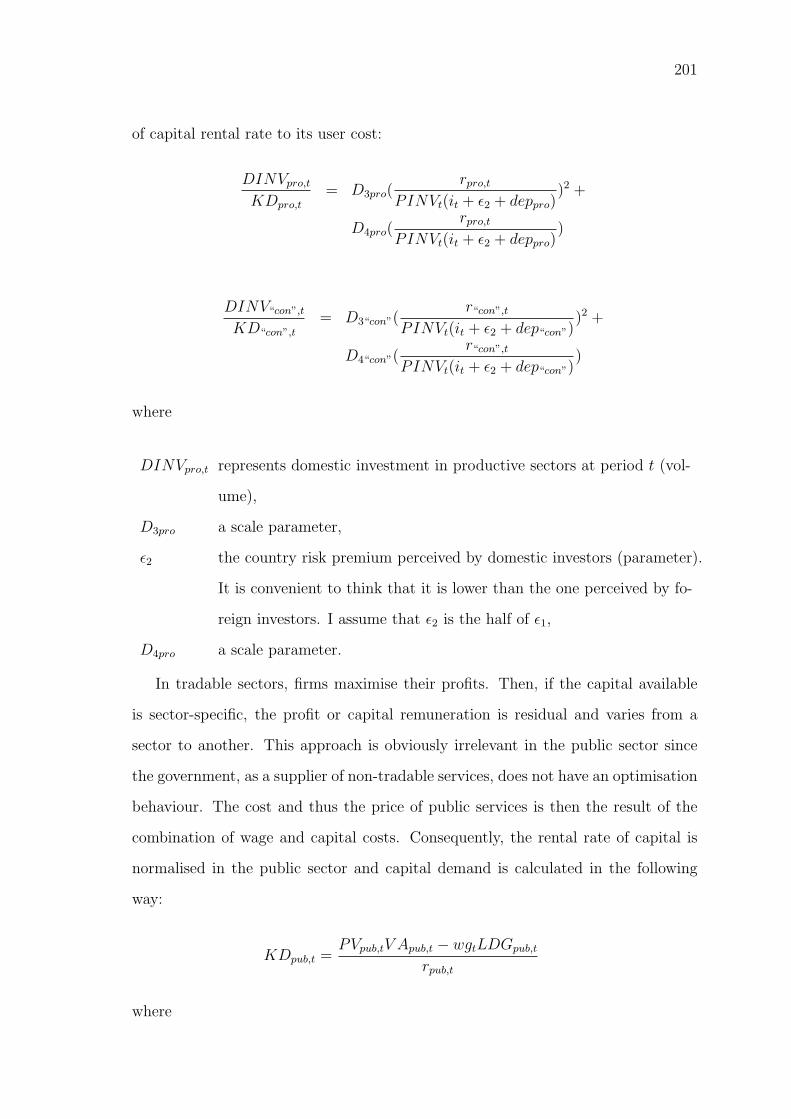
201

of capital rental rate to its user cost:

DINVpro,tKDpro,t

= D3pro(rpro,t

PINVt(it + ε2 + deppro))2 +

D4pro(rpro,t

PINVt(it + ε2 + deppro))

DINV“con”,t

KD“con”,t

= D3“con”(r“con”,t

PINVt(it + ε2 + dep“con”))2 +

D4“con”(r“con”,t

PINVt(it + ε2 + dep“con”))

where

DINVpro,t represents domestic investment in productive sectors at period t (vol-

ume),

D3pro a scale parameter,

ε2 the country risk premium perceived by domestic investors (parameter).

It is convenient to think that it is lower than the one perceived by fo-

reign investors. I assume that ε2 is the half of ε1,

D4pro a scale parameter.

In tradable sectors, firms maximise their profits. Then, if the capital available

is sector-specific, the profit or capital remuneration is residual and varies from a

sector to another. This approach is obviously irrelevant in the public sector since

the government, as a supplier of non-tradable services, does not have an optimisation

behaviour. The cost and thus the price of public services is then the result of the

combination of wage and capital costs. Consequently, the rental rate of capital is

normalised in the public sector and capital demand is calculated in the following

way:

KDpub,t =PVpub,tV Apub,t − wgtLDGpub,t

rpub,t

where

202 III. When Migrant Remittances Are Not Everlasting, How Can Morocco Make Up?

PVpub,t is the value added price of sector pub at period t,

wgt the public wage at period t (exogenous),

LDGpub,t the labour demand of sector pub at period t.

Therefore, the evolution of capital stock in public sectors can not agree with

the updating mechanism of capital stock in private sectors, and investment in non-

tradable sectors is endogenously determined by the model:

V ARKDt+1 = KD“edu”,t+1 −KD“edu”,t

As well, I need to add updating mechanisms for the following exogenous variables.

Over time, rural population LSRt grows at the exogenous population growth rate

gLSR, net of migration to urban areas MIGt and of international migration from

rural areas EMRt.

LSRt+1 = LSRt(1 + gLSR)−MIGt − EMRt

Urban population LSUt grows at the exogenous growth rate gLSU . It receives internal

migrants from rural areas MIGt and sends migrants abroad EMUt.

LSUt+1 = LSUt(1 + gLSU) +MIGt − EMUt

Migrant stock at period t is updated periodically with current migrant flows.

This means that migrant stock at each period is composed of several generations of

migrants that obviously have different remitting behaviours. Assuming that there

is only three migrant generations, one should expect that new migrants remit more

because they have the strongest ties with the family left behind. In contrast, the

second generation that later brought spouses and children in the process of family

reunification has lost some of its attachment to the country of origin, but still remits

in order to support the parents left behind. The amount remitted is lower than the

203

amount it should remit if all the family was still behind. The third generation of

migrants is supposed to be highly integrated in the country of destination and barely

remits. To sum up, the remitting behaviour depends on migrant generations that are

determined by the length of migration. However, the duration of living abroad can

not be reproduced in sequential dynamic models because they do not accommodate

calculations that involve variables from an indefinite long past. Therefore, some

simplifications need to be done. I present the adjustment mechanism of rural

and urban migrant stocks in the following way: I assume that rural and urban

migrant stocks of each period are composed of three generations according to the

age of migrants and that the first generation always receives current migrants. This

assumption is plausible since 74% of current migrant flows are aged between 15 and

29, according to Erf and Heering (2002). And, after years of migration, those young

migrants pass to the second and third generations of older migrants. At the base

year and for lack of data, I postulate that rural and urban migrant stocks have the

same age distribution: 35% of migrants are aged between 15 and 29, 42% between

30 and 44, and 23% more than 45 (Erf and Heering, 2002). At the following period,

a fraction of the first generation looses some of its attachment to the home country

and is added to the second generation. As well, a fraction of the second generation

becomes more disconnected from the family left behind and is added to the third

generation.

STKR1,t+1 = STKR1,t(1− χ1) + EMRt

for the first generation of rural migrants and:

STKU1,t+1 = STKU1,t(1− χ1) + EMUt

for the first generation of urban migrants, where

STKR1,t is the first generation of rural migrants at period t

204 III. When Migrant Remittances Are Not Everlasting, How Can Morocco Make Up?

EMRt the flow of rural migrants at period t,

STKU1,t the first generation of urban migrants at period t

EMUt the flow of urban migrants at period t,

χ1 the proportion of the first generation that passes periodically to the

second generation. Assuming that migrants who are 29 years old at

t will pass to the second generation at t+ 1 and that the number of

migrants aged between 25 and 29 is equally distributed between age

brackets, this parameter will be equal to 13%.

Now, the second generation of migrants at the following period is given by:

STKR2,t+1 = STKR2,t(1− χ2) + χ1STKR1,t

for rural migrants and,

STKU2,t+1 = STKU2,t(1− χ2) + χ1STKU1,t

for urban ones. where

χ2 is the proportion of the second generation that passes periodically to

the third one. Assuming that migrants who are 44 years old at t will

pass to the third generation at t+ 1 and that the number of migran-

ts aged between 30 and 44 is equally distributed between age bracke-

ts, this parameter will be equal to 7%.

Finally, the evolution of the third generation is given by:

STKR3,t+1 = STKR3,t + χ2STKR2,t

STKU3,t+1 = STKU3,t + χ2STKU2,t

205

The first generation of migrants remits to support the family left behind. Since

remittances are motivated by altruism, the remittance rate by migrant rises with his

income in the country of destination and decreases with the family real disposable

income10. The remittance rate for rural and urban households is respectively given

by:

RR“hr”,t = V1“hr”(Y D“hr”,t

CPIRt

)γ1“hr”wiγ2“hr”t

RR“hu”,t = V1“hu”(Y D“hu”,t

CPIUt)γ1“hu”wiγ2“hu”

t

where

RRh,t is the remittance rate to household h at period t,

V1h a scale parameter,

Y Dh,t the disposable income of household h at period t,

CPIRt the consumer price index in rural areas at period t,

CPIUt the consumer price index in urban areas at period t,

γ1,h the elasticity of remittance rate with respect to household h’s income

(-4.2% according to Bouhga-Hagbe, 2004),

wit the international wage rate at period t (exogenous),

γ2,h the elasticity of remittance rate with respect to the international wage

(1.8% according to Bouhga-Hagbe, 2004).

I arbitrarily assume that an individual belonging to the second generation of

10 Tables III.12, III.13 and III.14 in Appendix C present some selected results of the sensitivityanalysis on selected combinations of remittance elasticities with respect to household real incomeand with respect to the international wage. As expected, the results are not sensitive to the changeof remittance elasticity with respect to the international wage because the latter is kept exogenousall along the model. By contrast, the change of remittance elasticity with respect to householdreal income alter the results. A lower elasticity implies a smaller reaction of remittances tohousehold real income. Remittances increase or decrease less, for the same change of householdreal income. A higher elasticity generally increases the reaction of remittances to a changein household real disposable income. However, the results of the forthcoming simulations arequalitatively the same.

206 III. When Migrant Remittances Are Not Everlasting, How Can Morocco Make Up?

migrants remits the half of what it is supposed to remit, i.e. the half of the remittance

rate by migrant, and that the third generation does not remit at all. Therefore, the

value of remittances REMh,t received by household h at period t is:

REM“hr”,t = RR“hr”,tSTKR1,t + 1/2RR“hr”,tSTKR2,t

for the rural household and:

REM“hu”,t = RR“hu”,tSTKU1,t + 1/2RR“hu”,tSTKU2,t

for the urban household. The parameters χ1 and χ2 will be subject, later on, to a

shock (a rise of 20%) in order to reflect how the restriction of Western immigration

policies or permanent migration reduce the amount of remittances and thus affect

the Moroccan economy.

Migratory movements involve financial costs (travel cost, search for an apart-

ment, search for a job...) and psychological costs (change of the way of life,

adaptation to a new culture and a new community...). However, the more people

migrate to a particular destination, the more these costs are likely to decline.

The existence of migrant networks improves the access to information by potential

migrants left behind. For example, old migrants help reducing search costs regarding

jobs and housing, providing additional insurance in case of anticipated events... The

relation between migration costs and migrant networks is described as follows11:

MCt = V3(TSTKt)ν

where

11 Tables III.15, III.16 and III.17 in Appendix C present some results of the sensitivity analysis forselected value of migration cost elasticity with respect the total migrant stock. The higher theelasticity is, the greater migration costs react to the change of migrant stock. With a higherelasticity, migration costs decrease or increase more. The results show that when migration costsfall more, rural and urban emigration flows generally rise more, and vice versa. However, thechange of migration flows is so close to the results of the model simulations reported below.

207

MCt represents migration costs at period t,

V3 a scale parameter,

TSTKt the total stock of migrants at period t:

TSTKt = STKR1,t+STKR2,t+STKR3,t+STKU1,t+STKU2,t+STKU3,t

ν the elasticity of migration costs with respect to the total stock of mi-

grants (=-1.5).

The stock of internal migrants to urban areas at the following period ISTKt+1

is equal to the current stock to which is added the current internal migration flow:

ISTKt+1 = ISTKt +MIGt

Another adjustment equation is required for both domestic and external public

debts. The stock of domestic public debt at the following period SDDt+1 is equal to

the current stock SDDt to which are added the interest rate on the current stock it

and the accumulated debt during the current period DDt. Besides, at each period,

an adjustment variable for internal debt IAt is introduced so that to keep the ratio

of internal debt to GDP fixed and avoid infinite growth of interest rates paid by the

government. The same adjustment mechanism prevails for the external public debt

SFDt12.

SDDt+1 = (1 + it)SDDt +DDt − IAt

SFDt+1 = (1 + i∗t )SFDt + FDt − EAt12 Internal and external public debt are respectively fixed to 56% and 15% of GDP (Ministry of

Finance, Rabat).

208 III. When Migrant Remittances Are Not Everlasting, How Can Morocco Make Up?

The remaining exogenous variables evolve according to an average annual growth

rate calculated over 5 or 10 years, depending on the availability of the data (See

Appendix A). For instance, the evolution of public expenditures and investment is

given by:

Gi,t+1 = Gi,t(1 + gG)

INV Gt+1 = INV Gt(1 + gIG)

where

Gi,t represents government expenditures on good i at period t,

gG the average annual growth rate of government expenditures,

gIG the average annual growth rate of public investment in infrastructure.

3 Simulation Experiments

The long-term tendency goes against the maintenance or increase of remittances.

This is due to restrictive immigration policies especially in Europe and to the basic

immigration tendencies: permanent installation of Moroccans in the immigration

countries, family reunification, naturalisation, integration, ageing, and the succession

of generations living abroad. Is this fear of remittance shortage justified? I answer

this question by allowing a reduction in the number of migrants expected to remit.

This shock, called SIM1, consists of a 20% rise in the erosion rate of the first

and second generation of migrants, χ1 and χ2. As long as this fear of remittance

scarcity is economically approved, what would be the best policies in order to take

profit from current flows? According to Hamdouch (2000), this could be done

by channelling remittances away from real estate to productive sectors in order

to guarantee the conditions for a sustainable growth. Another option consists of

reducing international transfer costs in order to increase the value of remittances

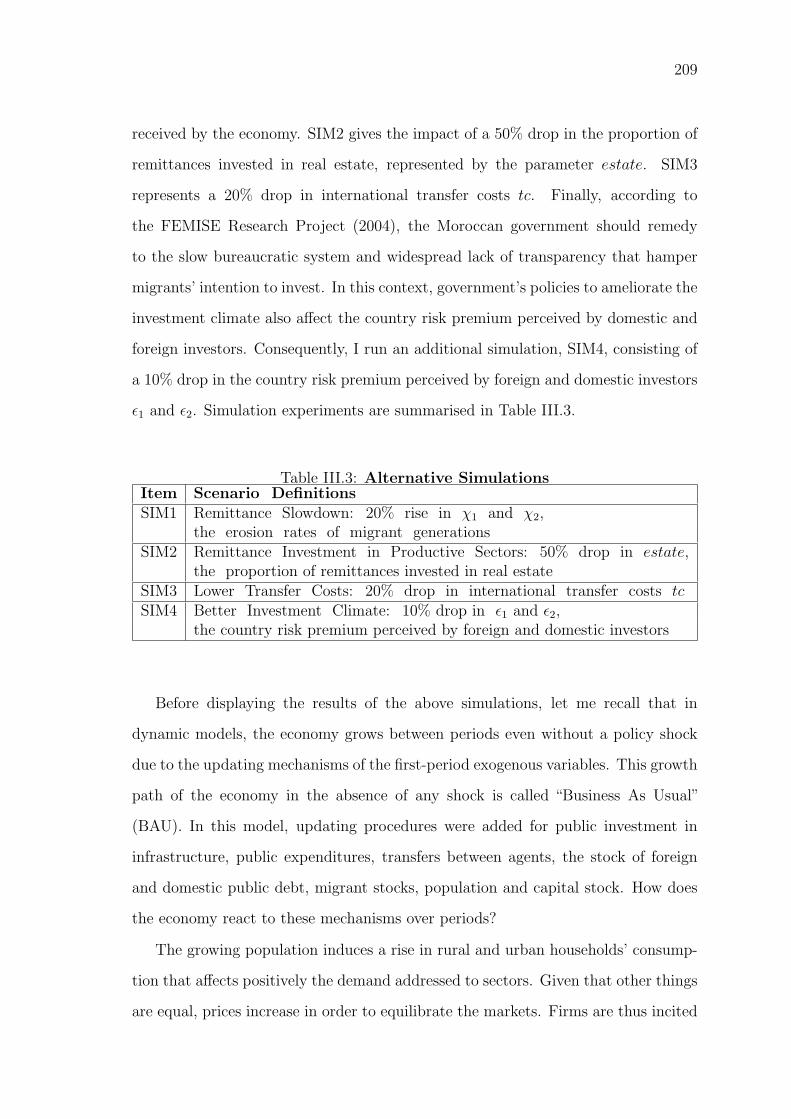
209

received by the economy. SIM2 gives the impact of a 50% drop in the proportion of

remittances invested in real estate, represented by the parameter estate. SIM3

represents a 20% drop in international transfer costs tc. Finally, according to

the FEMISE Research Project (2004), the Moroccan government should remedy

to the slow bureaucratic system and widespread lack of transparency that hamper

migrants’ intention to invest. In this context, government’s policies to ameliorate the

investment climate also affect the country risk premium perceived by domestic and

foreign investors. Consequently, I run an additional simulation, SIM4, consisting of

a 10% drop in the country risk premium perceived by foreign and domestic investors

ε1 and ε2. Simulation experiments are summarised in Table III.3.

Table III.3: Alternative SimulationsItem Scenario DefinitionsSIM1 Remittance Slowdown: 20% rise in χ1 and χ2,

the erosion rates of migrant generationsSIM2 Remittance Investment in Productive Sectors: 50% drop in estate,

the proportion of remittances invested in real estateSIM3 Lower Transfer Costs: 20% drop in international transfer costs tcSIM4 Better Investment Climate: 10% drop in ε1 and ε2,

the country risk premium perceived by foreign and domestic investors

Before displaying the results of the above simulations, let me recall that in

dynamic models, the economy grows between periods even without a policy shock

due to the updating mechanisms of the first-period exogenous variables. This growth

path of the economy in the absence of any shock is called “Business As Usual”

(BAU). In this model, updating procedures were added for public investment in

infrastructure, public expenditures, transfers between agents, the stock of foreign

and domestic public debt, migrant stocks, population and capital stock. How does

the economy react to these mechanisms over periods?

The growing population induces a rise in rural and urban households’ consump-

tion that affects positively the demand addressed to sectors. Given that other things

are equal, prices increase in order to equilibrate the markets. Firms are thus incited

210 III. When Migrant Remittances Are Not Everlasting, How Can Morocco Make Up?

to produce more. This is translated in a higher economic growth (Table III.4). The

additional demand for labour creates a pressure on rural and urban labour markets.

Rural wage adjusts upward in order to balance rural labour market. Surprisingly,

unemployment increases in urban areas, in spite of higher labour demand. Indeed,

urban population grows not only accordingly to the population natural growth rate,

but also due to internal migration from rural areas. In other words, labour supply

growth exceeds the increase in labour demand so that unemployment rises. The wage

curve insures that real urban wage decreases following the rise of unemployment.

Furthermore, increasing prices raise the value of intermediary consumption by sector.

Given that wages also increase, production costs grow and ceteris paribus, capital

remuneration that is calculated residually decreases in most sectors. In sum, total

factor remuneration increases in rural areas, inducing a rise in rural household

income and a welfare13 improvement by about 0.5% of his consumption budget.

However, starting period 15, the price increase is such that rural household real

disposable income decreases as well as rural welfare by 5% of his consumption budget.

Despite the lower remuneration of urban labour and capital, urban household income

also grows. Indeed, urban household receives interest payments on his lending to

the government14. Given that other things are equal, the government borrows more

in order to meet its investment in infrastructures. This results in higher interest

payments to urban household and firms. Urban household welfare increases by

about 2% of his consumption budget.

The increasing rural wage dampens migration intentions. On the contrary,

urban individuals are motivated to leave the country. Additional migration of

urban individuals helps reduce migration costs due to the increased network effect.

Besides, urban household receives, as expected, a higher amount of remittances.

Rural household also receives migrant remittances, although a lower amount than

urban household, mainly because of the altruistic motive. It happens that rural

13 Households’ welfare is given by the equivalent variation (Equation 120 in Appendix C).14 Let me recall that in Morocco, only urban households and firms lend to the government

(Abdelkhalek and Zaoujal, 2004).

211

household’s real disposable income declines starting period 15, encouraging rural

migrants to remit more in order to support their family left behind. The total

amount of remittances grows and helps explain, besides economic growth, the rise

of GNP. Given that other things are equal, it also induces an appreciation of the

real exchange rate15. On the one hand, the appreciated real exchange rate hampers

exports. On the other hand, it lowers the price of the foreign good in domestic

currency and promotes imports. While the “nominal” exchange rate appreciation16

should stimulate FDI due to profit repatriation, the diminishing rental rate of capital

impedes FDI flows in almost all sectors. Domestic investment also decreases for the

same reason.

After the shock, the economy will have another growth path due to the

simultaneous effect of the shock and the updating mechanisms of the first-period

exogenous variables. Consequently, the analysis should be done with respect to the

BAU growth path. In other words, the value of a given variable at period t after

the shock should be compared to its value at period t before the shock.

3.1 SIM1: Remittance Slowdown

A 20% rise in the erosion rate of migrant stocks has its first immediate impact on

household income. When migrant stock is eroded, fewer rural and urban migrants

will remit in the following period, leading, ceteris paribus, to a drop in rural and

urban households’ income (Table III.5). In addition, a part of remittances enters

households’ total savings and helps fund the domestic public debt. Since the

amount of money remitted decreases, the government will be less able to borrow

domestically and thus will have to pay a smaller amount of interest rates to the urban

household and firms. Consequently, urban household income decreases after the

15 The price of a unit of foreign currency in domestic currency.16 Let me recall that this is a real model. All variables are expressed in terms of GDP deflator

that stands for the numeraire. I only use the term “nominal exchange rate” for convenience tooutline the conversion unit of profits in foreign currency. However, since the real exchange rate(in terms of the numeraire) appreciates, it is also true to say that the “nominal” exchange rateor the conversion unit decreases.

212 III. When Migrant Remittances Are Not Everlasting, How Can Morocco Make Up?

Table III.4: The BAU Growth PathPercentage Change with Respect to the Base Year

t t+5 t+10 t+15 t+20Economic growthReal GDP at factor cost 0.00 1.47 3.46 4.71 5.13Real GNP 0.00 4.99 10.07 15.09 20.16Real wageRural 0.00 11.84 14.39 13.76 10.76Urban 0.00 -1.15 -1.47 -1.85 -2.64Unemployment 0.00 26.12 40.94 52.64 62.53Migration flowsRural 0.00 -12.01 -13.68 -13.42 -11.61Urban 0.00 29.12 63.28 94.68 128.02Internal 0.00 -40.04 -53.42 -59.02 -61.59Migration costs 0.00 -30.78 -53.28 -66.84 -75.59Households’ real disposable incomeRural 0.00 2.14 1.51 -0.08 -2.54Urban 0.00 1.50 2.98 3.73 3.59RemittancesTo rural household 0.00 7.94 22.95 40.04 62.84To urban household 0.00 17.25 47.78 84.22 129.34External tradeTotal export volume 0.00 -5.13 -9.19 -15.92 -25.80Total import volume 0.00 4.69 6.73 7.51 7.26Real exchange rate 0.00 -2.18 -2.32 -2.16 -1.77Total investment volumeAverage rental rate of capital 0.00 -6.28 -10.31 -14.15 -18.12FDI 0.00 -0.02 -0.05 -0.08 -0.12Domestic investment 0.00 -5.82 -12.64 -21.81 -32.68Source: Author’s calculations.

simultaneous drop of remittances and interest rates received from the government.

Given this evolution of households’ income, it is not surprising to see households’

consumption budget and welfare reduced. Rural and urban households’ welfare

maximum decreases with respect to the BAU growth path at the last period,

respectively by 0.64% and 0.85% of their consumption budget. If all prices remain

constant with respect to the BAU growth path, households will consume less goods

and services, inducing ceteris paribus a drop in total internal demand addressed to

each industry. Producers should reduce their production in order to meet the falling

demand.

Since the proportion of remittances not consumed is saved and channelled to

investment, one should expect, after the fall in the number of migrants who remit, a

drop in domestic investments by destination of all sectors, and especially in real

213

estate. Since the real estate sector is so integrated in the economy by highly

consuming intermediate inputs from other sectors, the real estate contraction further

helps reduce the demand addressed to sectors. However, domestic investment

becomes more profitable in some sectors because, as it will be shown below, the rental

rate of capital increases with respect to the investment aggregate price (agriculture,

mining industry, textile and clothing, leather industry, chemistry, rubber and plastic,

metallurgy, radios and TV, medical instruments, manufacture of other transport

means). In these sectors, domestic investment increases, and consequently the

volume of production, in spite of lower domestic demand. But finally, the overall

economic activity slows down with respect to the BAU growth path. GNP decreases

more than GDP due to lower remittances. On the one hand, the contraction of the

overall urban activity induces a drop of urban labour demand. Consequently, urban

unemployment rate increases, inducing a drop in urban real wage. On the other

hand, the expansion of the agricultural sectors stimulates rural labour demand.

Rural wage adjusts upward in order to balance the market.

Remittances to Morocco are computed in the BoP as current transfers. Since

external savings are constant for a given period, the drop in remittances should be

compensated by a decrease of the payments to the rest of the world. Therefore,

a depreciation of the real exchange rate is necessary. On the one hand, the

depreciated real exchange rate boosts exports. On the other hand, it raises the

price of imports in domestic currency and thus affects upward the composite price

of tradable goods. This results in higher consumer price indexes in rural and urban

areas. Domestic agents prefer then to rely on domestic products. Total import

volume decreases. It happens that the above-expanding sectors compete the most

with imports. Therefore, when imports become more expensive, domestic agents

consume mostly domestic products and sectors that initially highly compete with

imports expand. In those sectors, labour demand thus increases and, given that

other things are equal, the physical marginal productivity of capital as well as capital

remuneration increases.

214 III. When Migrant Remittances Are Not Everlasting, How Can Morocco Make Up?

The rise in rural consumer price index decreases rural real wage. The depreciated

“nominal” exchange rate also raises the wage of international migrants in domestic

currency. With the “nominal” exchange rate depreciation and the real wage drop,

rural and urban people are motivated to migrate. At each period, the network

effect increases with the accumulation of migrant flows, and reduces migration costs.

This further stimulates migration in the following period. Despite the increase of

migration flows, the total value of remittances continues to shrink because at each

period, fewer migrants are supposed to remit. Internal migration first decreases

because the rural real wage increases with respect to the urban expected real

wage. However, it starts increasing after period 15 when the rural real wage further

decreases.

The“nominal”exchange rate depreciation reduces the value of repatriated profits

in foreign currency and consequently discourages FDI. After few periods, the

increasing domestic investment in some of the above-mentioned sectors (agriculture,

leather industry, rubber and plastic, metallurgy) is more than compensated by falling

FDI. In total, the aggregate volume of capital invested in these sectors decreases.

Given that other things are equal, the initially expanded sectors shrink. In sum,

it turns out that the drop in capital invested in the different sectors is higher than

the fall in labour demand so that the marginal productivity of capital, and ceteris

paribus the return on capital, increases.

The segmentation of the savings market better draws the allocation of investment

between sectors, by allowing different types of savings to finance different invest-

ments. While domestic investment is driven by the differential between the sectoral

rental rate of capital and the aggregate price of investment, foreign investment is

triggered by the differential between the domestic and international rental rate

of capital, and public investment is exogenous because it stems from a public

decision. Therefore, there is no reason at all to have the same evolution for these

different types of investments with respect to the BAU growth path. Domestic

investment could be rising in some sectors and foreign investment decreasing due to

215

the “nominal” exchange rate depreciation (such as agriculture, textile and clothing,

chemistry, rubber and plastic, metallurgy, manufacture of other transport means).

Therefore, the evolution of total investment in these sectors is ambiguous: it depends

on the magnitude of each investment flow. The results show that the change

in domestic investment outweighs the change in foreign investment. Without a

segmentation of the savings market, investment by destination of all sectors will

have the same determinants and the results will absolutely be different from above

because investment determines the volume of capital used in the production process

and, ceteris paribus, the volume of production. Depending on the evolution of the

production in the different sectors, the economy will grow or shrink, affecting the

demand for labour and factor remuneration.

Table III.5: SIM1: Remittance SlowdownPercentage Change with Respect to the BAU Growth Path

t t+5 t+10 t+15 t+20Economic growthReal GDP at factor cost 0.00 -0.04 -0.13 -0.27 -0.46Real GNP 0.00 -0.08 -0.17 -0.29 -0.47Real wageRural 0.00 -0.03 -0.15 -0.32 -0.54Urban 0.00 -0.04 -0.07 -0.10 -0.17Unemployment 0.00 0.24 0.31 0.42 0.55Migration flowsRural 0.00 0.42 0.75 1.01 1.29Urban 0.00 0.71 1.15 1.55 2.01Internal 0.00 -0.24 -0.17 -0.05 0.05Migration costs 0.00 -0.06 -0.30 -0.58 -0.88Households’ real disposable incomeRural 0.00 -0.31 -0.65 -0.99 -1.33Urban 0.00 -0.32 -0.59 -0.85 -1.13RemittancesTo rural household 0.00 -3.05 -5.24 -6.28 -6.49To urban household 0.00 -2.77 -4.12 -4.37 -4.01External tradeTotal export volume 0.00 0.40 0.93 1.16 1.21Total import volume 0.00 -0.42 -0.73 -1.04 -1.37Real exchange rate 0.00 0.28 0.42 0.53 0.64Total investment volumeAverage rental rate of capital 0.00 0.04 0.22 0.47 0.59FDI 0.00 -0.55 -0.85 -1.18 -1.59Domestic investment 0.00 -0.30 -0.61 -1.02 -1.55

Source: Author’s calculations.

216 III. When Migrant Remittances Are Not Everlasting, How Can Morocco Make Up?

3.2 SIM2: Remittance Investment in Productive Sectors

As mentioned earlier, the proportion of remittances invested in real estate is

considered exogenous because the main purpose of sending money to Morocco is to

support the family left behind and/or to build a large new house offering the family

more convenient living, privacy and safety that were virtually absent in traditional

dwellings (de Haas, 2003; FEMISE, 2004). This means that investment in real

estate is driven by altruistic motives and not by profitability, like investment in

other sectors. Real estate absorbs 80% of investments by MRA in their country of

origin. However, Hamdouch (2000) noticed a change in the investment intentions

of the migrants interviewed, who plan to accord, from now on, only 36% of their

investment projects to real estate, mainly because they have intensively invested

in real estate. How does this change in MRA’s investment behaviour affect the

Moroccan economy?

A 50% drop in the proportion of remittances invested in real estate should

raise the proportion of remittances going to productive sectors and thus, domestic

investment in productive sectors. Given that other things are equal, this should lead

to a contraction of the construction sector and to a expansion of productive sectors.

Surprisingly, the vast majority of productive sectors shrink, negatively affecting the

overall economic activity (Table III.6). But this does not look odd anymore when one

looks deeply to the structure of the construction sector: intermediary consumption

accounts for 66% of the production value. So, when investment is reduced, inducing

ceteris paribus a contraction of this sector, producers cut down their consumption

of intermediary inputs, given the existing complementarity between production and

intermediary consumption. Thus, internal demand addressed to the different sectors

decreases, and producers choose to restrain their production. Only the following

sectors (agriculture, food industry, editing, furniture and non financial services) are

not affected because they offer no or little intermediary inputs to the real estate

sector.

The expanding sectors increase rural and urban labour demand. This causes

217

rural wage to rise and urban unemployment rate to fall in order to balance rural and

urban labour markets. The wage curve guarantees that real urban wage increases

following the lower unemployment rate. Given that other things are equal, the

lower labour demand in the contracted sectors induces a drop in the marginal

productivity of capital, and ceteris paribus a fall in the rental rate of capital that

negatively affects overall capital remuneration. The downward evolution of capital

remuneration reduces rural household income, consumption budget and welfare.

Welfare deterioration with respect to the BAU growth path reaches -0.68% of

rural household’s consumption budget. However, urban household income rises and

his welfare maximum improves at period 6 by 0.08% of his consumption budget.

Lower consumption further depresses the demand addressed to the different sectors,

whatever the goods are imported or produced domestically. Given that other things

are equal, producers lower their prices. After some periods, agriculture is also

affected by diminishing consumption. Labour demand decreases in rural areas

and rural wage falls in order to equilibrate the market. Later on, the initially

expanding urban sectors are touched as well. Urban labour demand then decreases

and unemployment increases. Real urban wage falls, as expected. Now, urban

household income also decreases with respect to the BAU growth path, and so does

his welfare. Welfare deterioration reaches 0.21% of his conusmption budget at the

final period.

Migration intentions to foreign countries are dampened with the wage improve-

ment. When fewer people migrate, in comparison with the BAU growth path, the

network effect is lessened and migration becomes more expensive. This further

discourages international migration. However, since internal migration costs are

supposed constant, the wage differential between rural and urban areas stimulates

internal migration. Although lower migration is expected to reduce the amount of

money remitted, this is only true, over some periods, for urban household. Indeed,

in accordance with the altruistic motive, rural migrants remit a greater amount

because rural household’s real disposable income falls. But in sum, the total amount

218 III. When Migrant Remittances Are Not Everlasting, How Can Morocco Make Up?

of remittances increases, inducing an appreciation of the real exchange rate in

order to maintain external savings fixed. The competitiveness of local producers

on international markets is thus deteriorated. While one expects that the “nominal”

exchange rate appreciation would have a stimulating effect on FDI, the results show

that this positive effect is counterbalanced by the detrimental role of a lower rental

rate of capital on FDI intentions in the different sectors. By contrast, the drop of

the aggregate price of investment compensates the negative evolution of the rental

rate of capital over some periods, so that domestic investment increases until period

15. The positive evolution of remittances also induces a lower drop of GNP, when

compared to GDP.

The predictions of this shock are unexpected. Scholars think that the allocation

of migrant investment to productive sectors should promote economic growth by

allowing a better productivity growth. However, it appears that there is a strong

demand effect that comes into play. This demand effect is related to the linkages

that transmit the negative impact of a particular shock on the production of the

real estate sector to the other ones, through lower intermediary consumption.

3.3 SIM3: Lower Transfer Costs

As shown in section 2, the cost and delay of transfers are high. I evaluate here the

impact of a 20% drop in international transfer costs and look if this could constitute

a good opportunity to take the maximum profit from remittances before their long-

term downward evolution.

When transfer costs decrease, households receive a larger value of remittances

with respect to the BAU growth path, that increases their income, consumption

budget and welfare (Table III.7). Welfare improvement is maximum at the last

period, reaching 0.16% of the consumption budget for rural household and 0.2% for

urban household.

Furthermore, as long as a fraction of remittances is invested, the drop in transfer

costs should, ceteris paribus, boost domestic investment in all sectors, and mostly

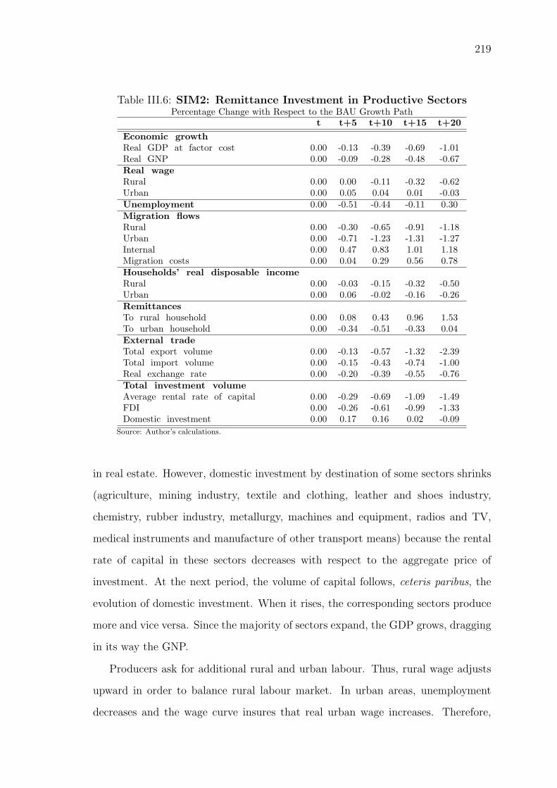
219

Table III.6: SIM2: Remittance Investment in Productive SectorsPercentage Change with Respect to the BAU Growth Path

t t+5 t+10 t+15 t+20Economic growthReal GDP at factor cost 0.00 -0.13 -0.39 -0.69 -1.01Real GNP 0.00 -0.09 -0.28 -0.48 -0.67Real wageRural 0.00 0.00 -0.11 -0.32 -0.62Urban 0.00 0.05 0.04 0.01 -0.03Unemployment 0.00 -0.51 -0.44 -0.11 0.30Migration flowsRural 0.00 -0.30 -0.65 -0.91 -1.18Urban 0.00 -0.71 -1.23 -1.31 -1.27Internal 0.00 0.47 0.83 1.01 1.18Migration costs 0.00 0.04 0.29 0.56 0.78Households’ real disposable incomeRural 0.00 -0.03 -0.15 -0.32 -0.50Urban 0.00 0.06 -0.02 -0.16 -0.26RemittancesTo rural household 0.00 0.08 0.43 0.96 1.53To urban household 0.00 -0.34 -0.51 -0.33 0.04External tradeTotal export volume 0.00 -0.13 -0.57 -1.32 -2.39Total import volume 0.00 -0.15 -0.43 -0.74 -1.00Real exchange rate 0.00 -0.20 -0.39 -0.55 -0.76Total investment volumeAverage rental rate of capital 0.00 -0.29 -0.69 -1.09 -1.49FDI 0.00 -0.26 -0.61 -0.99 -1.33Domestic investment 0.00 0.17 0.16 0.02 -0.09

Source: Author’s calculations.

in real estate. However, domestic investment by destination of some sectors shrinks

(agriculture, mining industry, textile and clothing, leather and shoes industry,

chemistry, rubber industry, metallurgy, machines and equipment, radios and TV,

medical instruments and manufacture of other transport means) because the rental

rate of capital in these sectors decreases with respect to the aggregate price of

investment. At the next period, the volume of capital follows, ceteris paribus, the

evolution of domestic investment. When it rises, the corresponding sectors produce

more and vice versa. Since the majority of sectors expand, the GDP grows, dragging

in its way the GNP.

Producers ask for additional rural and urban labour. Thus, rural wage adjusts

upward in order to balance rural labour market. In urban areas, unemployment

decreases and the wage curve insures that real urban wage increases. Therefore,

220 III. When Migrant Remittances Are Not Everlasting, How Can Morocco Make Up?

migration flows are dampened. The network effect is then reduced, inducing a

rise in migration costs. Moreover, when the economy receives a larger amount

of remittances, an appreciation of the real exchange rate is necessary in order

to increase the payments to the rest of the world and maintain external savings

constant. The “nominal” exchange rate appreciation reduces the value of the

international wage in domestic currency and besides higher migration costs, further

discourages international migration. Fewer people migrate, and the less will be the

amount of remittances in the following period.

On the one hand, the real exchange rate appreciation restrains export compet-

itiveness on international markets, inducing a drop in total export volume. On

the other hand, it decreases the relative price of imports in domestic currency,

and thus encourages domestic agents to consume cheaper imported products. It

happens that the above-contracted sectors compete the most with imports. Given

that other things are equal, producers facing lower internal demand are obliged to

reduce their sales. The contracted sectors release labour, and ceteris paribus, the

marginal productivity of capital as well as the rental rate of capital go down. This

explains the drop of investment by destination of these sectors.

FDI, triggered by the differential between the domestic and international return

on capital, is more profitable in almost all sectors (in comparison with the BAU

growth path) due to the “nominal” exchange rate appreciation. This is however not

the case of domestic investment that rises only in some sectors. Therefore, the total

volume of capital invested in each sector depends on the magnitude of each kind

of investment financed by different sources of savings. This is how the assumption

about a segmentation of the savings market affects the result.

Now, should transfer costs be reduced in the short run? What about the effect

of a late implementation of this measure? I answer this question by simulating

an additional shock, SIM3B, that explores the simultaneous impact of permanent

migration and lower international transfer costs, i.e the combination of SIM1 and

SIM3 (Table III.8). I find that permanent migration reduces the positive effect

221

Table III.7: SIM3: Lower Transfer CostsPercentage Change with Respect to the BAU Growth Path

t t+5 t+10 t+15 t+20Economic growthReal GDP at factor cost 0.02 0.04 0.07 0.11 0.14Real GNP 0.04 0.05 0.07 0.09 0.11Real wageRural 0.01 0.04 0.08 0.11 0.15Urban 0.03 0.01 0.02 0.02 0.03Unemployment -0.22 -0.10 -0.11 -0.13 -0.15Migration flowsRural 0.00 -0.18 -0.18 -0.19 -0.21Urban 0.00 -0.27 -0.26 -0.31 -0.36Internal 0.00 0.03 -0.03 -0.05 -0.05Migration costs 0.00 0.07 0.13 0.18 0.22Households’ real disposable incomeRural 0.14 0.15 0.18 0.21 0.25Urban 0.16 0.15 0.17 0.21 0.24RemittancesTo rural household -0.59 -0.69 -0.86 -1.02 -1.19To urban household -0.66 -0.73 -0.91 -1.09 -1.29External tradeTotal export volume -0.11 -0.19 -0.17 -0.12 -0.05Total import volume 0.23 0.16 0.19 0.22 0.26Real exchange rate -0.18 -0.08 -0.07 -0.08 -0.08Total investment volumeAverage rental rate of capital 0.04 -0.04 -0.09 -0.09 -0.15FDI 0.36 0.18 0.21 0.26 0.32Domestic investment 0.16 0.15 0.21 0.28 0.36

Source: Author’s calculations.

of lower transfer costs on household income. Rural and urban households’ income

increase over the first periods by less than SIM3 and so does households’ consumption

budget. Households’ demand motivates producers to adjust upward their production

and this promotes economic growth. Economic performance is however inferior

to the one obtained when SIM3 is run alone. In addition, the negative effect of

permanent migration on the amount remitted compensates the positive effect of

lower transfer costs. On the BoP level, the drop in the amount remitted induces a

depreciation of the real exchange rate that encourages exports and discourages more

expensive imports. The “nominal” exchange rate depreciation dampens FDI because

of lower profit repatriation. On the household level, decreasing remittances reduce

households’ income and welfare. On the one hand, domestic investment financed

by remittances falls. On the other hand, private consumption decreases. Producers

222 III. When Migrant Remittances Are Not Everlasting, How Can Morocco Make Up?

adjust their production downward in order to meet the lower demand. But the

slowdown of economic activity is lower than SIM1. Wages decrease following the

lower demand for labour and people are motivated to leave the country. In sum,

if this option should be undertaken, this has to be done before the slowdown of

remittances.

Table III.8: SIM3B: Remittance Slowdown and Lower Transfer CostsPercentage Change with Respect to the BAU Growth Path

t t+5 t+10 t+15 t+20Economic growthReal GDP at factor cost 0.02 0.00 -0.06 -0.17 -0.32Real GNP 0.04 -0.04 -0.10 -0.20 -0.30Real wageRural 0.01 0.01 -0.07 -0.21 -0.39Urban 0.03 -0.03 -0.05 -0.08 -0.13Unemployment -0.22 0.15 0.20 0.29 0.40Migration flowsRural 0.00 0.24 0.57 0.83 1.08Urban 0.00 0.45 0.90 1.24 1.65Internal 0.00 -0.21 -0.20 -0.09 0.00Migration costs 0.00 0.02 -0.17 -0.41 -0.67Households’ real disposable incomeRural 0.14 -0.17 -0.48 -0.79 -1.09Urban 0.16 -0.18 -0.42 -0.65 -0.90RemittancesTo rural household -0.59 -3.71 -6.04 -7.21 -7.58To urban household -0.66 -3.47 -4.98 -5.41 -5.24External tradeTotal export volume -0.11 0.22 0.70 1.01 1.17Total import volume 0.23 -0.26 -0.55 -0.82 -1.12Real exchange rate -0.18 0.21 0.35 0.45 0.55Total investment volumeAverage rental rate of capital 0.04 0.00 0.13 0.37 0.49FDI 0.36 -0.38 -0.64 -0.93 -1.28Domestic investment 0.16 -0.15 -0.41 -0.75 -1.20

Source: Author’s calculations.

3.4 SIM4: Better Investment Climate

There is a widespread perception that migrants might invest in their country of

origin if they possessed the necessary information and were encouraged to do so.

The increased allocation of remittances for private investment could then contribute

to sustained and higher economic growth. In this regard, measures to enhance the

223

investment climate characterised by a slow bureaucratic system and widespread lack

of transparency should help (FEMISE, 2004). Such measures influence the country

risk premium. Its improvement can perfectly reflect the policies adopted by the

government in order to attract investments. For this reason, I assess the impact

of a 10% drop in the country risk premium perceived by domestic investors. As

pointed out earlier, the risk premium perceived by local investors is lower than

the one perceived by foreign investors because the formers are more familiar with

investment procedures and business atmosphere in their country. However, when

the country risk premium perceived by local investors is improved, foreigners will

also have a better perception of the investment climate that should trigger foreign

investment.

As expected, foreign and domestic investors have greater confidence in in-

vestment: this is reflected by a simultaneous increase of domestic and foreign

investments in comparison with the BAU growth path (Table III.9). Given that

other things are equal, the capital used in the production of all sectors rises in the

next period. The production follows, ceteris paribus, the evolution of the capital

volume. This is translated in higher GDP and GNP. Since domestic producers offer

their production on local and international markets, the production growth should be

reflected in increased exports and local supply. A depreciation of the real exchange

rate is therefore necessary to guarantee the competitiveness of local producers on

international markets and stimulate exports. I recall that export expansion increases

total factor productivity growth in the corresponding sectors. Imports also increase

in order to maintain external savings fixed.

Rural and urban labour demand increase with the expansion of rural and urban

sectors. Rural wage rises, as expected in order to balance rural labour market. In

urban areas, unemployment falls and real urban wage rises, as predicted by the wage

curve. While one should expect a drop in international migration from rural and

urban areas after the increase in rural and urban wages, it seems that the exchange

rate depreciation counterbalances the downward effect of the wage improvement

224 III. When Migrant Remittances Are Not Everlasting, How Can Morocco Make Up?

on migration intentions. However, this is only true over the first periods. Later

on, international migration flows decrease. The network effect strengthens with

migrant number and is inversely related to migration costs. Internal migration

is dampened, as expected. Households’ income and welfare increase following

the improvement of labour remuneration. Welfare improvement is the greatest

here, reaching respectively about 2% and 1.55% of rural and urban hoseholds’

consumption budget at the last period. Since remittances are motivated by altruism,

migrants remit a smaller amount. That is why GNP grows less than GDP.

Households consumption further stimulates the economic activity. The growing

labour demand is such that the marginal productivity of capital increases as well

as, ceteris paribus, capital remuneration. This further encourages FDI and domestic

investment.

The improvement of the risk premium reduces the possibilities for the government

to borrow domestically by channelling a part of local savings to investment. But

the government’s investment objective in infrastructures is met thanks to the

improvement of public savings. Indeed, the amount of direct taxes and imports

tariffs collected by the government induces a rise in public savings. This leads

to a downward adjustment of the indirect tax rate in order to keep the ratio of

government savings to GDP fixed.

I should also point out that this policy needs to be settled before the cut down in

remittances. Indeed, I run SIM4B that is a combination of SIM1 and SIM4 (Table

III.10) and find that permanent migration reduces the economic performance due

to the improvement of the country risk premium, because permanent migration is

translated in lower remittances, and thus, lower domestic investment. It also reduces

households’ welfare with respect to SIM4: permanent migration causes a negative

economic growth that induces a lower labour demand. Consequently, wages fall

down in comparison to SIM4, dragging in their way households’ income and welfare.

The economy receives now a smaller amount of remittances because of permanent

migration (SIM1) and the altruistic motive (SIM4). Therefore, the real exchange

225

Table III.9: SIM4: Better Investment ClimatePercentage Change with Respect to the BAU Growth Path

t t+5 t+10 t+15 t+20Economic growthReal GDP at factor cost 0.00 0.49 1.12 1.67 2.12Real GNP 0.00 0.22 0.68 1.05 1.29Real wageRural 0.00 0.60 1.14 1.64 2.09Urban 0.00 0.00 0.00 0.04 0.10Unemployment 0.00 -0.65 -1.64 -2.22 -2.47Migration flowsRural 0.00 0.34 0.13 -0.03 -0.01Urban 0.00 0.43 -0.64 -1.50 -1.93Internal 0.00 -0.84 -0.77 -0.81 -0.97Migration costs 0.00 -0.16 -0.16 0.05 0.33Households’ real disposable incomeRural 0.00 0.38 0.78 1.12 1.37Urban 0.00 0.21 0.62 0.92 1.11RemittancesTo rural household 0.00 -1.47 -3.06 -4.43 -5.48To urban household 0.00 -0.61 -2.46 -4.18 -5.48External tradeTotal export volume 0.00 1.23 2.89 4.89 7.27Total import volume 0.00 0.01 0.46 0.81 0.93Real exchange rate 0.00 0.35 0.36 0.39 0.52Total investment volumeAverage rental rate of capital 0.00 0.09 0.31 0.66 1.08FDI 2.73 3.28 4.00 4.59 4.96Domestic investment 1.56 2.52 3.67 4.64 5.45

Source: Author’s calculations.

rate depreciates more in order to maintain external savings fixed. On the one hand,

the real exchange rate depreciation further boosts exports. On the other hand, it

raises the price of imported products in domestic currency. This is translated in

higher composite prices of tradable goods. Real urban wage decreases because the

wage increase is more than compensated by the growth of the urban consumer price

index.

4 Conclusion

This chapter tackles a debatable issue regarding the impact of remittances on the

Moroccan economy. Policy makers in less developed as well as developed countries

have implicitly assumed that remittances benefit the country of origin. Morocco has

226 III. When Migrant Remittances Are Not Everlasting, How Can Morocco Make Up?

Table III.10: SIM4B: Permanent Migration and Better Investment ClimatePercentage Change with Respect to the BAU Growth Path

t t+5 t+10 t+15 t+20Economic growthReal GDP at factor cost 0.00 0.45 0.99 1.40 1.67Real GNP 0.00 0.14 0.52 0.77 0.89Real wageRural 0.00 0.56 1.00 1.33 1.57Urban 0.00 -0.07 -0.06 -0.06 -0.06Unemployment 0.00 -0.41 -1.34 -1.83 -1.94Migration flowsRural 0.00 0.75 0.85 0.94 1.21Urban 0.00 1.14 0.46 -0.05 -0.06Internal 0.00 -1.08 -0.93 -0.85 -0.92Migration costs 0.00 -0.21 -0.45 -0.51 -0.51Households’ real disposable incomeRural 0.00 0.07 0.14 0.15 0.06Urban 0.00 -0.11 0.05 0.09 0.00RemittancesTo rural household 0.00 -4.50 -8.21 -10.56 -11.81To urban household 0.00 -3.37 -6.56 -8.55 -9.53External tradeTotal export volume 0.00 1.63 3.77 6.04 8.53Total import volume 0.00 -0.42 -0.24 -0.19 -0.39Real exchange rate 0.00 0.63 0.76 0.89 1.12Total investment volumeAverage rental rate of capital 0.00 0.09 0.54 1.12 1.67FDI 2.73 2.71 3.16 3.42 3.38Domestic investment 1.56 2.23 3.06 3.64 3.90

Source: Author’s calculations.

even used these possible benefits to underpin its emigration policy. But now, this is

not the main question. Surveys on Morocco showed that remittances have most of

the time been beneficial. The question is how to take the maximum profit from this

external source of funding in a way to enhance the development of this country and

cushion its transition to be gradually less dependent on remittances.

This chapter fills the gap in the Moroccan literature on remittances by assessing

the impact of remittances and their alternative uses. In this sense, it differs from the

work on Morocco that consists of surveys and studies on particular regions. It also

adds to the literature on MENA countries that have been generally ruled out in this

context, in spite of their high dependency on remittances. The main contribution

of this chapter is to model a segmentation of the savings market, where remittances

do not finance the same sectors as domestic investment or FDI. This is supposed to

227

better draw the reality since different sources of investment do not have the same

determinants and affect differently the sectors of destination.

The fear from the cut down of remittances seems to be justified. The overall

economic growth and households’ welfare are reduced. I use a dynamic CGE model

of the Moroccan economy, calibrated on the SAM of the year 1998, to investigate

policies allowing to take the best profit from current remittance flows. I simulate

the effects of a 50% drop in the proportion of remittances invested in real estate, a

20% drop in transfer costs and a 10% drop in the country risk premium perceived by

investors. Nonetheless, not all the policies proposed by surveys are advantageous.

Surprisingly, it turns out that the drop of the proportion of remittances invested

in real estate reduces economic growth and welfare. Indeed, the linkages between

construction and other sectors appear to be important so that a negative shock

on real estate production also affects others sectors through a drop in intermediary

demand addressed to them. Lower transfer costs and the improvement of the country

risk premium both lead to an overall activity growth and to welfare improvement,

still more pronounced in the second case.

228 III. When Migrant Remittances Are Not Everlasting, How Can Morocco Make Up?

III.A Appendix A: Data

The model is calibrated on the Moroccan SAM described in Appendix A of Chapter

1. I further decompose the SAM in order to distinguish between rural and urban

areas and take into account two categories of household: a rural household offering

his working hours to rural sectors and an urban household offering his working hours

to urban sectors17.

FDI flows are distributed between sectors according to data from the Moroccan

BoP of 1998. Even though the number of sectors considered in the SAM does not

match those of the BoP, the correspondence between sectors is easy to establish. The

repartition of the gross fixed capital formation between aggregate sectors is derived

from national accounts. The difference between total gross fixed capital formation

and FDI volume gives the volume of investment by domestic agents (households,

firms and the government). Public investment in infrastructure represents 3.5%

of GDP (author’s calculation from national accounts). In 1998, the public debt

represented 89% of GDP with 51% of GDP external and 38% internal (Ministry of

Finance, Rabat).

Finally, migration data are taken from several sources:

1- To quantify Moroccan emigration, I resort to the data published by the OECD in

2006 on immigrant inflows by nationality in some OECD countries. I approximate

Moroccan emigration by the flows of Moroccan migrants to their traditional

destinations in 1999, such as Belgium, France, Italy, the Netherlands and Spain.

The sum of these flows (63,200 migrants) is reported to the Moroccan working

population of 1999 in order to calculate the annual percentage of emigrants (0.6%).

I also use the stocks of Moroccan migrants in the previous selected countries in order

to approximate the stock of migrants necessary to the adjustment of the model in

the dynamic framework.

2- According to a report of the International Organisation of Migration (Erf and

17 For further details, see Appendix A in Chapter 2.

229

Heering, 2002), Moroccan emigration to European countries is more originated from

rural areas. Therefore, I suppose that 60% of the national emigration flow/stock

take place from rural areas and 40% from urban areas.

3- Agenor and El Aynaoui (2003) point out that each year, around 200,000 workers

migrate from rural to urban areas. This corresponds approximately to 4% of the

1999 rural working population.

For the majority of exogenous variables, I observed their evolution over 5 or 10

years, according to data availability, and calculated their average annual growth

rate. I retained respectively the following values for public expenditures and public

investment in infrastructure: 2.9%, 2.3%. The rural population natural growth rate

(2.6%) is taken from Agenor and El Aynaoui (2003). The urban population natural

growth rate (0.8%) is based on author’s calculations. For lack of data, minimum

consumption and exogenous transfers to and from households are updated according

to the population growth rate.

Finally, I report the values of some parameters imported from external sources:

the absolute value of the wage elasticity with respect to unemployment is fixed to

0.1 (See Chapter 2), transfer costs represent 9% of the amount of the transaction

(Barendse, Hiddink, Janszen and Stavast, 2006), the risk premium is fixed at 4.88%

(United States Agency for International Development (USAID)) and the capital

depreciation rate at 8% (Agenor and El Aynaoui, 2003). Armington and exports

elasticities, respectively 2 and -5, are borrowed from the literature on Morocco

(Lofgren et al., 1999; Rutherford et al., 1997).

230 III. When Migrant Remittances Are Not Everlasting, How Can Morocco Make Up?

III.B Appendix B: Mathematical Statement of

the Model

Set indices are given by lower-case Latin letters as subscripts to variables and

parameters. Parameters are represented with lower-case Latin letters or lower-case

Greek letters, endogenous variables with upper-case Latin letters without a bar,

exogenous variables with upper-case Latin letters with a bar.

Sets

j ∈ J Sectorsi ∈ I Products (=J)tr ∈ TR ⊂ J Tradable sectorsntr ∈ NTR ⊂ J Non-tradable sectorsps ∈ PS ⊂ J Private sectorspub ∈ PUB ⊂ J Public sectorspro ∈ PRO ⊂ PS Productive sectorsru ∈ RU ⊂ PS Rural private sectorsup ∈ UP ⊂ PS Urban private sectorsag ∈ AG Agentsda ∈ DA ⊂ AG Domestic agentsh ∈ H ⊂ AG Householdst ∈ T Time period

Parameters

αps Share parameter of the CES value added of sector psσps Elasticity of substitution between labour and capital (positive)lpub Labour share in public value added (Leontief)kpub Capital share in public value added (Leontief)ioj Share of intermediary consumption in the production (Leontief) of se-

ctor jvj Share of value added in the production (Leontief) of sector jaiji,j Intermediary consumption of good i by unit of production of sector jB1 Scale parameter of the CET function of the rural population$1 Share parameter of this functionε1 Elasticity of transformation between international rural migrants and

national workers (negative)

231

B2 Scale parameter of the CET function of the rural population that de-cides to stay in Morocco

$2 Share parameter of this functionε2 Elasticity of of transformation between internal migrants and rural w-

orkers (negative)B3 Scale parameter of the CET function of the urban population$3 Share parameter of this functionε3 Elasticity of of transformation between international urban migrants

and urban workers (negative)imc Internal migration costsηag Share of capital remuneration received by agent agφag Share of labour remuneration received by agent agtc transfer costsϑag Part of interest rates on domestic public debt going to agent agV1h Parameter in the international remittance rate function of household hυ Part of stock variation financed by foreign firmsγ1,h Elasticity of international remittance rate with respect to household h’s

real incomeγ2,h Elasticity of international remittance rate to household h with respect to

the international wageV2 Parameter in the remittance rate function from urban to rural householdγ3 Elasticity of internal remittance rate with respect to rural household real

incomeψh Household’s h propensity to savetyh Direct tax rate on household h’s incometye Direct tax rate on firms’ incometxj Indirect tax rate on sector j productstmtr Import tariff rate on product trtetr Export tariff rate on product trς Export externality parameter (positive)C1tr Scale parameter of the CET production functionδ1tr Share parameter of this functionκ1tr Transformation elasticity of the CET production function (negative)ϕtr Price elasticity of export demandC2tr Scale parameter of the Armington CES functionδ2tr Share parameter of this functionκ2tr Substitution elasticity of the Armington function (positive)βi,h Budgetary share of good i in the supernumerary income of household hµi Share of product i in total investment valueD Scale parameter of the wage curveζ The absolute value of the wage elasticity with respect to unemploymentθ1i Weight of commodity i in the consumer price indexθ2i,“hr” Weight of commodity i in rural consumer price indexθ2i,“hu” Weight of commodity i in urban consumer price index

232 III. When Migrant Remittances Are Not Everlasting, How Can Morocco Make Up?

θj Share of sector j value added in GDP at factor costχ1 Erosion rate of the first generation of migrantsχ2 Erosion rate of the second generation of migrantsdepps Capital depreciation rate of sector psD1ps Parameter in the FDI equationD2ps Parameter in the FDI equationε1 The country risk premium perceived by foreign investorsε2 The country risk premium perceived by domestic investorsD3ps Parameter in the equation of domestic investment by households and firmsD4ps Parameter in the equation of domestic investment by households and firmsV3 Parameter in the international migration cost functionν Elasticity of international migration costs to the stock of international mig-

rants (negative)gG Growth rate of government expendituresgIG Growth rate of public investment in infrastructuregLSR Natural growth rate of rural populationgLSU Natural growth rate of urban populationF Parameter in the domestic public debt functionξ Elasticity of domestic public debt financed by households and firms with

respect to the risk factor (positive)cons Part of international remittances going to consumptionestate Part of international remittances (net of the amount consumed) going to

real estate

Endogenous Variables

a) Prices

wrt Rural wage ratewut The wage rate paid by urban private sectorswgt The wage rate paid by urban public sectorswit International wage rate, in foreign currencywnt National wage ratewugt Average urban wage ratewat Expected urban wage raterj,t Capital return in sector jr∗t International average rate of capitalPVj,t Value added price of sector jPLj,t Producer price of local product jPDj,t Market price of local product j sold on the domestic marketPj,t Production price of sector jPCj,t Market price of the composite good belonging to sector jPwmtr,t International import price of product tr, in foreign currency

233

Pwetr,t International export price of product tr, in foreign currencyPMtr,t Domestic price of the imported good trPEtr,t Producer price of the exported good trPfobtr,t FOB price of the exported good trPINVt Aggregate price of investmentet Nominal exchange rate (the price of a unit of foreign currency in

domestic currency)it Interest rate on domestic public debti∗t Interest rate on foreign public debtCPIt Consumer price indexCPIRt Consumer price index in rural areasCPIUt Consumer price index in urban areasPindext GDP deflator, numeraire

b) Production

XSj,t Production of sector j (volume)Aps,t Export externality shift parameter in the production of sector psV Aj,t Value added of sector j (volume)DIi,j,t Intermediary demand of product i by sector j (volume)CIj,t Total intermediary consumption of sector j (volume)

c) Factors of production

KDj,t Capital demand by sector j (volume)LDRru,t Labour demand by rural sector ru (volume)LDUup,t Labour demand by urban private sector up (volume)LDGpub,t Labour demand by public sector pub (volume)LSRt Rural populationLSUt Urban populationut Urban unemployment rate

d) Migration

NATt Rural workers who decide to stay in MoroccoEMRt Rural emigrant flowNATRt Rural workers who decide to stay in rural areasMIGt Rural migrant flow towards urban areasNATUt Urban workers who decide to stay in urban areasEMUt Urban emigrant flowSTKR1,t The first generation of rural migrantsSTKU1,t The first generation of urban migrants

234 III. When Migrant Remittances Are Not Everlasting, How Can Morocco Make Up?

STKR2,t The second generation of rural migrantsSTKU2,t The second generation of urban migrantsSTKR3,t The third generation of rural migrantsSTKU3,t The third generation of urban migrantsTSTKt Total stock of international migrantsISTKt Stock of internal migrants from rural to urban areasMCt International migration costs

e) Income/Savings

Yag,t Agent ag’s incomeYWRh,t Income of household h, excluding remittancesY Dh,t Disposable income of household hY DWRh,tDisposable income of household h, excluding remittancesPROFt The proportion of capital remuneration repatriated by foreign firmsSag,t Agent ag’s savingsTag,ag,t Transfers between agentsRRh,t Remittance rate to household hIRt Internal remittance rate from urban to rural householdREMh,t Migrant remittancesDDt Domestic public debtKt Adjustment variable in the debt equationFDt Foreign public debtSDDt Stock of domestic public debtSFDt Stock of foreign public debtIAt Internal debt reimbursementEAt External debt reimbursement

f) Tax revenues

TIj,t Indirect taxes on product jTIMtr,t Import tariffs on product trTIEtr,t Export tariffs on product tradjt Compensatory tax

g) External trade

EXStr,t Export supply of product tr (volume)DOMj,t Domestic production of sector j sold on the domestic market (volume)Qj,t Supply of composite product belonging to sector j (volume)EXDtr,t Export demand of product tr (volume)Mtr,t Import demand of product tr (volume)

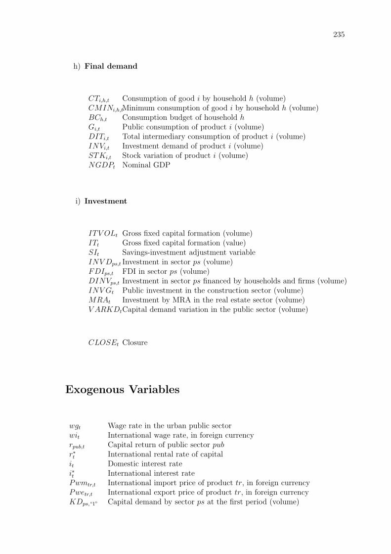
235

h) Final demand

CTi,h,t Consumption of good i by household h (volume)CMINi,h,tMinimum consumption of good i by household h (volume)BCh,t Consumption budget of household hGi,t Public consumption of product i (volume)DITi,t Total intermediary consumption of product i (volume)INVi,t Investment demand of product i (volume)STKi,t Stock variation of product i (volume)NGDPt Nominal GDP

i) Investment

ITV OLt Gross fixed capital formation (volume)ITt Gross fixed capital formation (value)SIt Savings-investment adjustment variableINV Dps,t Investment in sector ps (volume)FDIps,t FDI in sector ps (volume)DINVps,t Investment in sector ps financed by households and firms (volume)INV Gt Public investment in the construction sector (volume)MRAt Investment by MRA in the real estate sector (volume)V ARKDtCapital demand variation in the public sector (volume)

CLOSEt Closure

Exogenous Variables

wgt Wage rate in the urban public sectorwit International wage rate, in foreign currencyrpub,t Capital return of public sector pubr∗t International rental rate of capitalit Domestic interest ratei∗t International interest ratePwmtr,t International import price of product tr, in foreign currencyPwetr,t International export price of product tr, in foreign currencyKDps,“1” Capital demand by sector ps at the first period (volume)

236 III. When Migrant Remittances Are Not Everlasting, How Can Morocco Make Up?

CMINi,h,“1”Minimum consumption of product i by household h (volume)Gi,“1” Public consumption of product i, at the first period (volume)STKi,t Stock variation of product i (volume)Srow,t External savingsLSR“1” Rural population, at the first periodLSU“1” Urban population, at the first periodSTKR1,“1” The first generation of rural migrants, at the first periodSTKU1,“1” The first generation of urban migrants, at the first periodSTKR2,“1” The second generation of rural migrants, at the first periodSTKU2,“1” The second generation of urban migrants, at the first periodSTKR3,“1” The third generation of rural migrants, at the first periodSTKU3,“1” The third generation of urban migrants, at the first periodTSTK“1” Total stock of international migrants, at the first periodISTK“1” Stock of internal migrants, at the first periodSDD“1” Stock of internal public debt, at the first periodSFD“1” Stock of external public debt, at the first periodINV G“1” Public investment in the construction sector, at the first period (volume)CLOSEt ClosurePindext GDP deflator, numeraire

All transfers between agents except direct taxes paid by households and firms.Transfers to and from households as well as minimum consumption by productare fixed at the first period and updated exogenously between periods with thepopulation growth rate.

Equations

Rural Sectors

XSru,t = V Aru,t/vru (A1)

CIru,t = ioruXSru,t (A2)

DIi,ru,t = aiji,ruCIru,t (A3)

V Aru,t = Aru,t[αruLDR(σru−1)/σruru,t + (1− αu)KD

(σru−1)/σruru,t ]σru/(σru−1) (A4)

LDRru,t/KDru,t = (αru

1− αrurru,twrt

)σru (A5)

237

Urban Private Sectors

XSup,t = V Aup,t/vup (A6)

CIup,t = ioupXSup,t (A7)

DIi,up,t = aiji,upCIup,t (A8)

V Aup,t = Aup,t[αupLDU(σup−1)/σupup,t + (1− αup)KD

(σup−1)/σupup,t ]σup/(σup−1) (A9)

LDUup,t/KDup,t = (αup

1− αuprup,twut

)σup (A10)

Public Sectors

XSpub,t = V Apub,t/vpub (A11)

CIpub,t = iopubXSpub,t (A12)

DIi,pub,t = aiji,pubCIpub,t (A13)

V Apub,t = KDpub,t/kpub (A14)

LDGpub,t = lpubV Apub,t (A15)

KDpub,t =PVpub,tV Apub,t − wgtLDGpub,t

rpub,t(A16)

Migratory Flows

LSRt = B1[$1NAT(ε1−1)/ε1t + (1−$1)EMR

(ε1−1)/ε1t ]ε1/(ε1−1) (A17)

EMRt

NATt= (

$1

1−$1

wit−1et−1(1−MCt−1)

wnt−1/CPIt−1

)−ε1 (A18)

NATt = B2[$2NATR(ε2−1)/ε2t + (1−$2)MIG

(ε2−1)/ε2t ]ε2/(ε2−1) (A19)

238 III. When Migrant Remittances Are Not Everlasting, How Can Morocco Make Up?

MIGt

NATRt

= ($2

1−$2

wat−1(1− imc)/CPIUt−1

wrt−1/CPIRt−1

)−ε2 (A20)

LSU t = B3[$3NATU(ε3−1)/ε3t + (1−$3)EMU

(ε3−1)/ε3t ]ε3/(ε3−1) (A21)

EMUtNATUt

= ($3

1−$3

wit−1et−1(1−MCt−1)

wat−1/CPIUt−1

)−ε3 (A22)

Households and Firms

Y“hr”,t =∑ru

wrtLDRru,t + η“hr”

∑j

rjKDj,t +∑da

T “hr”,da,t +

etT “hr”,”row”,t + IRtISTKt + (1− tc)REM“hr”,t (A23)

Y“hu”,t = (1− φrow)[∑up

wutLDUup,t +∑pub

wgtLDGpub,t] +

η“hu”

∑j

rj,tKDj,t +∑da

T “hu”,da,t + etT “hu”,”row”,t +

ϑ“hu”(itSDDt) + (1− tc)REM“hu”,t (A24)

YWR“hr”,t =∑ru

wrtLDRru,t + η“hr”

∑j

rjKDj,t +∑da

T “hr”,da,t +

etT “hr”,”row”,t + IRtISTKt (A25)

YWR“hu”,t = (1− φrow)[∑up

wutLDUup,t +∑pub

wgtLDGpub,t] + η“hu”

∑j

rj,tKDj,t +∑da

T “hu”,da,t + etT “hu”,”row”,t + ϑ“hu”(itSDDt) (A26)

Y DWR“hr”,t = YWR“hr”,t(1− ty“hr”)− T “hr”,“hr”,t −T “hu”,“hr”,t − T “fm”,“hr”,t − etT “row”,“hr”,t (A27)

Y DWR“hu”,t = YWR“hu”,t(1− ty“hu”)− T “hr”,“hu”,t − T “hu”,“hu”,t −T “fm”,“hu”,t − etT “row”,“hu”,t − IRtISTKt (A28)

Y D“hr”,t = Y“hr”,t(1− ty“hr”)− T “hr”,“hr”,t −T “hu”,“hr”,t − T “fm”,“hr”,t − etT “row”,“hr”,t (A29)

239

Y D“hu”,t = Y“hu”,t(1− ty“hu”)− T “hr”,“hu”,t − T “hu”,“hu”,t −T “fm”,“hu”,t − etT “row”,“hu”,t − IRtISTKt (A30)

REM“hr”,t = RR“hr”,tSTKR1,t + 1/2RR“hr”,tSTKR2,t (A31)

REM“hu”,t = RR“hu”,tSTKU1,t + 1/2RR“hu”,tSTKU2,t (A32)

RR“hr”,t = V1“hr”(Y D“hr”,t

CPIRt

)γ1“hr”witγ2“hr” (A33)

RR“hu”,t = V1“hu”(Y D“hu”,t

CPIUt)γ1“hu”wit

γ2“hu” (A34)

IRt = V2(Y D“hr”,t

CPIRt

)γ3 (A35)

Sh,t = ψhY DWRh,t (A36)

BC“hr”,t = Y“hr”,t(1− ty“hr”)− T “hr”,“hr”,t − T “hu”,“hr”,t −T “fm”,“hr”,t − etT “row”,“hr”,t − S“hr”,t −(1− cons“hr”)(1− ty“hr”)(1− tc)REM“hr”,t (A37)

BC“hu”,t = Y“hu”,t(1− ty“hu”)− T “hr”,“hu”,t − T “hu”,“hu”,t −T “fm”,“hu”,t − etT “row”,“hu”,t − IRtISTKt − S“hu”,t −(1− cons“hu”)(1− ty“hu”)(1− tc)REM“hu”,t (A38)

Y“fm”,t = (1− η“hr” − η“hu” − η“gv” − η“row” − PROFt)∑j

rj,tKDj,t +∑da

T “fm”,da,t + etT“fm”,”row”,t + (1− ϑ“hu”)(itSDDt) (A39)

PROFt =

∑ps FDIps,t

ITV OLt(A40)

S“fm”,t = Y“fm”,t(1− tye)− T “hr”,“fm”,t − T “hu”,“fm”,t −T“fm”,“fm”,t − etT“row”,“fm”,t (A41)

240 III. When Migrant Remittances Are Not Everlasting, How Can Morocco Make Up?

The Government

TItr,t = txtradjt(Ptr,tXStr,t − PEtr,tEXStr,t) +

txtradjt(1 + tmtr)etPmwtr,tMtr,t (A42)

TIntr,t = txntradjtPLntr,tXSntr,t (A43)

TIMtr,t = tmtretPwmtr,tMtr,t (A44)

TIEtr,t = tetrPEtr,tEXStr,t (A45)

T“gv”,h,t = tyhYh,t (A46)

T“gv”,“fm”,t = tyeY“fm”,t (A47)

Y“gv”,t = η“gv”

∑j

rj,tKDj,t +∑tr

TIMtr,t +∑tr

TIEtr,t +∑j

TIj,t +∑h

T“gv”,h,t + T“gv”,“fm”,t + T“gv”,“gv”,t + etT“gv”,“row”,t (A48)

S“gv”,t = Y“gv”,t −∑i

PCi,tGi,t −∑da

T da,“gv”,t −

etT“row”,“gv”,t − itSDDt − eti∗tSFDt (A49)

External Trade

If EXStr,t EXStr,t−1,

Atr,t = Atr,t−1(EXStr,tEXStr,t−1

)ς (A50)

If EXStr,t ≤ EXStr,t−1

Atr,t = Atr,t−1 (A51)

XStr,t = C1tr[δ1trEXS(κ1tr−1)/κ1tr

tr,t + (1− δ1tr)DOM(κ1tr−1)/κ1tr

tr,t ]κ1tr/(κ1tr−1) (A52)

XSntr,t = DOMntr,t (A53)

241

EXStr,tDOMtr,t

= (δ1tr

1− δ1tr

PLtr,tPEtr,t

)κ1tr (A54)

EXDtr,t = EXDtr,t−1(Pwetr,tPfobtr,t

)ϕtr (A55)

Qtr,t = C2tr[δ2trM(κ2tr−1)/κ2tr

tr,t + (1− δ2tr)DOM(κ2tr−1)/κ2tr

tr,t ]κ2tr/(κ2tr−1) (A56)

Qntr,t = DOMntr,t (A57)

Mtr,t

DOMtr,t

= (δ2tr

1− δ2tr

PDtr,t

PMtr,t

)κ2tr (A58)

S“row”,t =∑tr

Pwmtr,tMtr,t + φrow

∑upwutLDUup,t +

∑pubwgtLDGpub,t

et

+(η“row” + PROFt)

∑j rj,tKDj,t

et+

∑ag

T “row”,ag,t + i∗tSFDt

−∑tr

Pfobtr,tEXStr,t −∑ag

T ag,row,t −∑

h(1− tc)REMh,t

et(A59)

Final Demand

CTi,“hr”,t = CMIN i,“hr”,t +βi,“hr”PCi,t

(BC“hr”,t −∑i

PCi,tCMIN i,“hr”,t) (A60)

CTi,“hu”,t = CMIN i,“hu”,t +βi,“hu”

PCi,t(BC“hu”,t −

∑i

PCi,tCMIN i,“hu”,t) (A61)

INVi,t = µiITt/PCi,t (A62)

DITi,t =∑i

aiji,jCIj,t (A63)

ITV OLt = ITt/PINVt (A64)

242 III. When Migrant Remittances Are Not Everlasting, How Can Morocco Make Up?

NGDPt =∑i

PCi,tGi,t +∑h

∑i

PCi,tCTi,h,t +∑i

PCi,tINVi,t +∑i

PCi,tSTKi,t +∑tr

etPfobtr,tEXDtr,t −∑tr

Pwmtr,tetMtr,t (A65)

Prices

lnwut

CPIUt= D − ζ lnut (A66)

wgt wut (A67)

wnt =wrt

∑ru LDRru,t + wut

∑up LDUup,t + wgt

∑pub LDGpub,t∑

ru LDRru,t +∑

up LDUup,t +∑

pub LDGpub,t

(A68)

wugt =wut

∑up LDUup,t + wgt

∑pub LDGpub,t∑

up LDUup,t +∑

pub LDGpub,t

(A69)

wat = wugt(1− ut) (A70)

rru,t =PVru,tV Aru,t − wrtLDRru,t

KDru,t

(A71)

rup,t =PVup,tV Aup,t − wutLDUup,t

KDup,t

(A72)

PVj,t =Pj,tXSj,t −

∑i PCi,tDIi,j,t

V Aj,t(A73)

PMtr,t = etPwmtr,t(1 + tmtr)(1 + txtradjt) (A74)

PEtr,t =etPfobtr,t(1 + tetr)

(A75)

PCtr,t =DOMtr,tPDtr,t +Mtr,tPMtr,t

Qtr,t

(A76)

PCntr,t = PDntr,t (A77)

243

PDj,t = PLj,t(1 + txjadjt) (A78)

Ptr,t =PLtr,tDOMtr,t + PEtr,tEXStr,t

XStr,t(A79)

Pntr,t = PLntr,t (A80)

PINVt =∏i

(PCi,tµi

)µi

(A81)

CPIt =∑i

θ1iPCi,t (A82)

CPIRt =∑i

θ2i,“hr”PCi,t (A83)

CPIUt =∑i

θ2i,“hu”PCi,t (A84)

Pindext =∑j

θjPVj,t (A85)

Dynamics

STKR1,t+1 = STKR1,t(1− χ1) + EMRt (A86)

STKU1,t+1 = STKU1,t(1− χ1) + EMUt (A87)

STKR2,t+1 = STKR2,t(1− χ2) + χ1STKR1,t (A88)

STKU2,t+1 = STKU2,t(1− χ2) + χ1STKU1,t (A89)

STKR3,t+1 = STKR3,t + χ2STKR2,t (A90)

STKU3,t+1 = STKU3,t + χ2STKU2,t (A91)

244 III. When Migrant Remittances Are Not Everlasting, How Can Morocco Make Up?

TSTKt = STKR1,t + STKR2,t + STKR3,t + (A92)

STKU1,t + STKU2,t + STKU3,t

ISTKt+1 = ISTKt +MIGt (A93)

KDps,t+1 = (1− depps)KDps,t + INV Dps,t (A94)

FDIps,tKDps,t

= D1ps(rps,t

etr∗t (it + ε1 + depps))2 + (A95)

D2ps(rps,t

etr∗t (it + ε1 + depps))

DINVps,tKDps,t

= D3ps(rps,t

PINVt(it + ε2 + depps))2 + (A96)

D4ps(rps,t

PINVt(it + ε2 + depps))

V ARKDt = KD“edu”,t −KD“edu”,t−1 (A97)

INV Dpro,t = DINVpro,t + FDIpro,t (A98)

INV D“con”,t = MRAt +DINV“con”,t + INV Gt + FDI“con”,t (A99)

SDDt+1 = (1 + it)SDDt +DDt − IAt (A100)

SFDt+1 = (1 + i∗t )SFDt + FDt − EAt (A101)

MCt = V3(TSTKt)ν (A102)

Gi,t+1 = Gi,t(1 + gG) (A103)

INV Gt+1 = INV Gt(1 + gIG) (A104)

LSRt+1 = LSRt(1 + gLSR)−MIGt − EMRt (A105)

LSUt+1 = LSU t(1 + gLSU) +MIGt − EMUt (A106)

245

Equilibrium Conditions and Closure

NATRt =∑ru

LDRru,t (A107)

(NATUt + (1− imc)MIGt)(1− ut) =∑up

LDUup,t +∑pub

LDGpub,t (A108)

Qi,t = Gi,t +DITi,t +∑h

CTi,h,t + INVi,t + STKi,t (A109)

EXStr,t = EXDtr,t (A110)

S“gv”,t +DDt + etFDt = V ARKDtPINVt + INV GtPINVt (A111)

DDt = Kt(F × εξ2)(S“hu”,t + (1− estate)(1− cons“hu”) (A112)

(1− ty“hu”)(1− tc)REM“hu”,t + S“fm”,t)

∑h

estate(1− consh)(1− tyh)(1− tc)REMh,t = MRAtPINVt (A113)

et(S“row”,t − FDt) =∑pro

FDIpro,tPINVt +

FDI“con”,tPINVt + υ∑i

STKi,tPCi,t (A114)

ITt +∑i

STKi,tPCi,t = etS”row”,t +∑da

Sda,t + (A115)∑h

(1− consh)(1− ty)(1− tc)REMh,t

ITV OLt = SIt(∑pro

INV Dpro,t + INV D“con”,t + V ARKDt) (A116)

CLOSEt = S“gv”,t/NGDPt (A117)

SDDt+1 = share1NGDPt+1 (A118)

246 III. When Migrant Remittances Are Not Everlasting, How Can Morocco Make Up?

etSFDt+1 = share2NGDPt+1 (A119)

EVh = (BCh,t −∑i

PCi,tCMINi,h,t)(

∏i PCOi∏i PCi,t

)βi,h

−

(BCOh −∑i

PCOiCMINOi,h) (A120)

247

III.C Appendix C: Sensitivity Analysis

Table III.11: Real GDP at Factor Cost For Selected Valuesof Export Externality Parameter

Percentage Change with Respect to the BAU Growth PathExternality Scenario t t+5 t+10 t+15 t+20

0.2 SIM1 0.00 -0.03 -0.07 -0.18 -0.34SIM2 0.00 -0.13 -0.38 -0.67 -0.98SIM3 0.02 0.04 0.08 0.11 0.16SIM4 0.00 0.57 1.37 2.12 2.80

0.05 SIM1 0.00 -0.06 -0.17 -0.33 -0.52SIM2 0.00 -0.13 -0.39 -0.70 -1.02SIM3 0.02 0.04 0.07 0.10 0.14SIM4 0.00 0.44 0.97 1.41 1.75

Source: Author’s calculations.

Table III.12: Real GDP at Factor Cost For Selected Combinationsof Remittance Elasticities

Percentage Change with Respect to the BAU Growth Pathγ1,h γ2,h Scenario t t+5 t+10 t+15 t+20-4.2 0.9 SIM1 0.00 -0.04 -0.13 -0.27 -0.46

SIM2 0.00 -0.13 -0.39 -0.69 -1.01SIM3 0.02 0.04 0.07 0.11 0.14SIM4 0.00 0.49 1.12 1.67 2.12

-4.2 3.6 SIM1 0.00 -0.04 -0.13 -0.27 -0.46SIM2 0.00 -0.13 -0.39 -0.69 -1.01SIM3 0.02 0.04 0.07 0.11 0.14SIM4 0.00 0.49 1.12 1.67 2.12

-2.1 1.8 SIM1 0.00 -0.05 -0.16 -0.34 -0.58SIM2 0.00 -0.13 -0.40 -0.71 -1.05SIM3 0.02 0.05 0.09 0.13 0.18SIM4 0.00 0.50 1.14 1.73 2.23

-8.4 1.8 SIM1 0.00 -0.03 -0.10 -0.20 -0.32SIM2 0.00 -0.13 -0.38 -0.66 -0.95SIM3 0.01 0.03 0.05 0.08 0.10SIM4 0.00 0.48 1.09 1.60 2.00

Notes: (1) γ1,h: Elasticity of international remittance rate with respect tohousehold h’s real income.(2) γ2,h: Elasticity of international remittance rate with respect to theinternational wage.Source: Author’s calculations.

Table III.13: Household Real Disposable IncomeFor Selected Combinations of Remittance Elasticities

Percentage Change with Respect to the BAU Growth Pathγ1,h γ2,h Scenario Household t t+5 t+10 t+15 t+20-4.2 0.9 SIM1 Rural 0.00 -0.31 -0.65 -0.99 -1.33

Urban 0.00 -0.32 -0.59 -0.85 -1.13SIM2 Rural 0.00 -0.03 -0.15 -0.32 -0.50

Urban 0.00 0.06 -0.02 -0.16 -0.26SIM3 Rural 0.14 0.15 0.18 0.21 0.25

Urban 0.16 0.15 0.17 0.21 0.24SIM4 Rural 0.00 0.38 0.78 1.12 1.37

Urban 0.00 0.21 0.62 0.92 1.11-4.2 3.6 SIM1 Rural 0.00 -0.31 -0.65 -0.99 -1.33

Urban 0.00 -0.32 -0.59 -0.85 -1.13SIM2 Rural 0.00 -0.03 -0.15 -0.32 -0.50

Urban 0.00 0.06 -0.02 -0.16 -0.26SIM3 Rural 0.14 0.15 0.18 0.21 0.25

Urban 0.16 0.15 0.17 0.21 0.24SIM4 Rural 0.00 0.38 0.78 1.12 1.37

Urban 0.00 0.21 0.62 0.92 1.11-2.1 1.8 SIM1 Rural 0.00 -0.38 -0.80 -1.22 -1.66

Urban 0.00 -0.39 -0.73 -1.09 -1.49SIM2 Rural 0.00 -0.03 -0.17 -0.39 -0.65

Urban 0.00 0.07 -0.01 -0.17 -0.35SIM3 Rural 0.17 0.18 0.23 0.27 0.33

Urban 0.19 0.18 0.22 0.27 0.33SIM4 Rural 0.04 0.45 0.93 1.37 1.76

Urban 0.00 0.25 0.74 1.13 1.42-8.4 1.8 SIM1 Rural 0.00 -0.17 -0.40 -0.60 -0.78

Urban 0.00 -0.18 -0.33 -0.45 -0.55SIM2 Rural 0.00 -0.15 -0.36 -0.57 -0.74

Urban 0.00 -0.08 -0.23 -0.37 -0.49SIM3 Rural 0.07 0.09 0.11 0.13 0.14

Urban 0.08 0.09 0.10 0.11 0.12SIM4 Rural 0.10 0.46 0.72 0.87 0.92

Urban 0.01 0.25 0.48 0.58 0.57Notes: (1) γ1,h: Elasticity of international remittance rate with respect to household h’sreal income.(2) γ2,h: Elasticity of international remittance rate with respect to the international wage.Source: Author’s calculations.

Table III.14: Households’ RemittancesFor Selected Combinations of Remittance Elasticities

Percentage Change with Respect to the BAU Growth Pathγ1,h γ2,h Scenario To Household t t+5 t+10 t+15 t+20-4.2 0.9 SIM1 Rural 0.00 -3.05 -5.24 -6.28 -6.49

Urban 0.00 -2.77 -4.12 -4.37 -4.01SIM2 Rural 0.00 0.08 0.43 0.96 1.53

Urban 0.00 -0.34 -0.51 -0.33 0.04SIM3 Rural -0.59 -0.69 -0.86 -1.02 -1.19

Urban -0.66 -0.73 -0.91 -1.09 -1.29SIM4 Rural 0.00 -1.47 -3.06 -4.43 -5.48

Urban 0.00 -0.61 -2.46 -4.18 -5.48-4.2 3.6 SIM1 Rural 0.00 -3.05 -5.24 -6.28 -6.49

Urban 0.00 -2.77 -4.12 -4.37 -4.01SIM2 Rural 0.00 0.08 0.43 0.96 1.53

Urban 0.00 -0.34 -0.51 -0.33 0.04SIM3 Rural -0.59 -0.69 -0.86 -1.02 -1.19

Urban -0.66 -0.73 -0.91 -1.09 -1.29SIM4 Rural 0.00 -1.47 -3.06 -4.43 -5.48

Urban 0.00 -0.61 -2.46 -4.18 -5.48-2.1 1.8 SIM1 Rural 0.00 -3.55 -6.22 -7.69 -8.30

Urban 0.00 -3.27 -4.93 -5.42 -5.25SIM2 Rural 0.00 0.03 0.17 0.44 0.79

Urban 0.00 -0.24 -0.52 -0.52 -0.27SIM3 Rural -0.35 -0.46 -0.60 -0.73 -0.88

Urban -0.40 -0.51 -0.68 -0.85 -1.04SIM4 Rural 0.00 -0.80 -1.79 -2.77 -3.67

Urban 0.00 -0.27 -1.51 -2.90 -4.14-8.4 1.8 SIM1 Rural 0.00 -2.41 -4.01 -4.55 -4.39

Urban 0.00 -2.13 -3.15 -3.19 -2.73SIM2 Rural 0.00 0.15 0.77 1.55 2.25

Urban 0.00 -0.48 -0.51 -0.13 0.34SIM3 Rural -0.90 -0.97 -1.16 -1.33 -1.49

Urban -0.99 -1.00 -1.17 -1.35 -1.53SIM4 Rural 0.00 -2.41 -4.72 -6.34 -7.24

Urban 0.00 -1.02 -3.71 -5.82 -7.03Notes: (1) γ1,h: Elasticity of international remittance rate with respect to household h’s realincome.(2) γ2,h: Elasticity of international remittance rate with respect to the international wage.Source: Author’s calculations.

Table III.15: Migration CostsFor Selected Values of Migration Cost Elasticity ν

Percentage Change with Respect to the BAU Growth Pathν Scenario t t+5 t+10 t+15 t+20

-0.75 SIM1 0.00 -0.03 -0.15 -0.28 -0.43SIM2 0.00 0.02 0.14 0.27 0.38SIM3 0.00 0.04 0.06 0.09 0.11SIM4 0.00 -0.08 -0.08 0.02 0.17

-3 SIM1 0.00 -0.11 -0.61 -1.17 -1.77SIM2 0.00 0.09 0.59 1.14 1.61SIM3 0.00 0.15 0.27 0.36 0.45SIM4 0.00 -0.32 -0.32 0.08 0.65

Notes: ν: Elasticity of international migration costs to the stock ofinternational migrants.Source: Author’s calculations.

Table III.16: Rural Emigration FlowFor Selected Values of Migration Cost Elasticity ν

Percentage Change with Respect to the BAU Growth Pathν Scenario t t+5 t+10 t+15 t+20

-0.75 SIM1 0.00 0.41 0.74 1.01 1.29SIM2 0.00 -0.30 -0.65 -0.90 -1.16SIM3 0.00 -0.17 -0.17 -0.19 -0.21SIM4 0.00 0.33 0.12 -0.04 -0.04

-3 SIM1 0.00 0.42 0.74 1.00 1.28SIM2 0.00 -0.30 -0.66 -0.91 -1.19SIM3 0.00 -0.18 -0.18 -0.19 -0.21SIM4 0.00 0.35 0.14 -0.01 -0.02

Notes: ν: Elasticity of international migration costs to the stock ofinternational migrants.Source: Author’s calculations.

Table III.17: Urban Emigration FlowFor Selected Values of Migration Cost Elasticity ν

Percentage Change with Respect to the BAU Growth Pathν Scenario t t+5 t+10 t+15 t+20

-0.75 SIM1 0.00 0.71 1.15 1.55 2.02SIM2 0.00 -0.71 -1.22 -1.29 -1.23SIM3 0.00 -0.27 -0.26 -0.31 -0.37SIM4 0.00 0.42 -0.66 -1.53 -1.99

-3 SIM1 0.00 0.71 1.15 1.53 2.00SIM2 0.00 -0.71 -1.23 -1.32 -1.29SIM3 0.00 -0.27 -0.26 -0.31 -0.36SIM4 0.00 0.44 -0.63 -1.46 -1.87

Notes: ν: Elasticity of international migration costs to the stock ofinternational migrants.Source: Author’s calculations.

Chapter IV

On The Relation Between Trade

Liberalisation and Migration in

Morocco

Morocco is in the bulk of the trade liberalisation process. The country is about to

achieve a free trade area with the EU by 2012 and has signed free trade agreements

with the US, Turkey and other Arab countries, at the same time as it adjusts its

trade policies to match the WTO rules. In this context, the major concern stems

from the potential labour market effects of integration and enlargement. A sketchy

analysis suggests that trade liberalisation should expand the low protected sectors

and contract the highly protected ones. If the expanding sectors are labour-intensive,

trade liberalisation will dampen unemployment rates. Given that unemployment is

the most important cause for migration in Morocco, it is true to think that trade

liberalisation may reduce migration incentives. This issue is of prime importance at

a time industrialised countries closed their doors to Southern workers for economic,

social and security reasons. Another concern is whether and to what extent Morocco

should pursue additional trade liberalisation: does the FTA with the EU promote

enough growth and employment in Morocco so that migration incentives decrease

or should the country carry on additional efforts for multilateral liberalisation?

251

252 IV. On The Relation Between Trade Liberalisation and Migration in Morocco

This chapter explores the link between trade liberalisation and migration in

Morocco. Because trade agreements involve substantial changes in prices, resource

allocation and income, and affect capital stock through savings as well as human

capital and technology, the analysis is done with a dynamic CGE model of the

Moroccan economy. Based on a robust and widely accepted modelling of agents’

behaviour, CGE models are able to provide a detailed description of the impact

of such shocks on the economy. A particular attention is given to Morocco and

the Euro-Mediterranean partnership at a time where illegal migration is a matter

of discordance between the EU and South-Mediterranean countries. Two trade

liberalisation scenarios are considered, the first corresponding to the FTA creation,

and the second dealing with multilateral liberalisation.

The relation between trade and migration has extensively been analysed on

both theoretical and empirical grounds. Factor mobility is a substitute for trade

if trade liberalisation allows factor price equalisation. Mundell (1957) showed that

trade and migration are substitutes in the standard HO model of trade with two

production factors under the usual assumptions: if labour migrates from the labour-

abundant country, the production of the exportable good will fall and the output of

the importable one will increase along traditional Rybczynski lines. Consequently,

trade will decline. Similarly, in the labour-scarce country, migration will boost

the production of the importable good and lead to a decline in the output of

the exportable one, and hence to a reduction in trade. However, the Mundell

model (1957) and related evidence have been questioned both at the theoretical

and empirical levels. In their literature review, Faini et al. (1999) clearly explain

how the conclusions of Mundell (1957) can be reversed simply by using more realistic

253

assumptions1.

Empirically, little is known about the effects of trade liberalisation on emigration

flows in developing countries. The available computational literature has focused,

for the most part, on US-Mexico migration patterns after the creation of the North

American Free Trade Agreement (NAFTA). Hill and Mendez (1984) show that a

removal of trade barriers reduces migration flows from Mexico to the US, but that

the reduction is fairly modest. By contrast, Robinson et al. (1993) argue that

trade liberalization in agriculture greatly increases rural-urban migration within

Mexico and migration from Mexico to the US, and that lower migration is only

possible if Mexico grows relative to the US and if it retains farm support programs.

Melchor del Rio and Thorwarth (2006) give support to Robinson et al. (1993) by

showing, using monthly data from 1966 to 2004, that greater trade flows cause larger

illegal migration from Mexico to the US. More recent works were interested in the

relation between trade liberalisation and emigration in Morocco. The CGE analyses

of Bouzahzah et al. (2007) and Cogneau and Tapinos (1995), based respectively on

1985 and 19802 data, both conclude that trade liberalisation did not help reduce

migration flows. By contrast, Faini and de Melo (1995) develop a macroeconometric

model calibrated for the year 1988 and show that trade liberalisation induces a

real exchange rate depreciation that, on the one hand, results in higher production

costs and lower supply, and on the other hand, boosts labour-intensive exports and

1 For example, when the difference in technology is allowed in a Ricardian framework and if therich country is more productive in the labour-intensive sector, it will export the labour intensivegood, and then display a higher wage. If labour mobility is now allowed, labour will migrate fromthe poor to the rich country, and, through standard Rybczynski effects, this will strengthen thespecialisation of the rich country in the labour-intensive sector. Specific-factors models can alsoinduce a relation between trade liberalisation and migration that is different from the standardHO model. Trade liberalisation reduces the price of the importable good and then depresses thedemand for labour, the mobile factor, in the import sector. Both the nominal wage and the realwage in terms of the exportable good fall. However, the real wage in terms of the importablegood will increase and this will be translated to the whole wage only if the weight of importablegoods in the consumption budget is high. Without being exhaustive, a final example concernfinancial-constraints models. Lopez and Schiff (1998) show that, when migrants are financiallyconstrained and unable to migrate due to migration costs, and if trade liberalisation raises thewage in the labour-abundant sending country according to the HO model, financial constraintswill be relaxed and, paradoxically, migration will increase.

2 Nevertheless, the SAM of Cogneau and Tapinos (1995) was updated by data on external tradeand taxation in 1990.

254 IV. On The Relation Between Trade Liberalisation and Migration in Morocco

labour demand. The second effect dominates so that trade liberalisation is found to

promote employment creation and thus discourage migration.

However, none of the previous works investigated the different impacts of trade

liberalisation on skilled and unskilled migration. In the standard HO model, and

given that Morocco is unskilled-labour abundant, it must export unskilled-labour

intensive goods and import skilled-labour intensive ones. In order to meet increasing

exports, labour demand of unskilled workers must rise and unskilled wage must

adjust upward to balance the labour market. In this context, international labour

mobility and trade liberalisation are substitutes. By contrast, if Moroccan imports

are skilled-labour intensive and when imports replace domestic production, skilled

labour demand decreases and so does the wage of skilled workers. Consequently,

skilled workers choose to leave. In this context, migration and trade liberalisation

are complements. Given that Morocco’s main trading partners are developed skilled-

abundant countries and since Moroccan imports mainly consist of capital and

technology goods, it is true to think that they are skilled-labour intensive. Therefore,

one would expect that unskilled migration decreases and skilled migration increases,

following tariff removal.

This chapter looks at the labour-market effects of Moroccan trade liberalisation

with a special interest in its impact on the skill-composition of migration. The

analysis is done with a CGE framework adapted to migration and trade liberal-

isation. International and internal migration are motivated by wage differentials

and the effect of urban unemployment rate on migration incentives is taken into

consideration. A sequential dynamic module is added making possible the allocation

of savings, including remittances, to investment. Therefore, the evolution of

migration flows also affects capital accumulation through skilled and unskilled

migrants’ abilities to remit. The model is calibrated on a disaggregated SAM of

2003, thus offering an updated analysis of this subject, in contrast to the previous

works. Indeed, the structure of Moroccan external trade displayed many changes

between the 1980s, where the country was still in the bulk of structural adjustment,

255

and 2000. Besides, the previous studies are characterised by a sectoral aggregation

level that is likely to hide the diversity of protection applied to the disaggregated

sectors, and thus affect winners and losers from liberalisation. Finally, and limiting

the comparison to the works using the same methodology, it is worth mentioning that

Bouzahzah et al. (2007) may have underestimated the impact of trade liberalisation

because their analysis was done in a static framework, neglecting the dynamic

effects of liberalisation coming from physical and human capital accumulation.

Nevertheless, the analysis was made in an imperfect competition framework with

scale economies, according to the new CGE literature following the work of Harris

(1984). Dynamic effects of trade liberalisation are deeply examined in Cogneau and

Tapinos (1995), but in a perfect competition framework.

Two trade liberalisation scenarios are considered, the first consisting of the

Morocco-EU FTA and the second of multilateral liberalisation. The simulations are

run twice, in a perfect and imperfect competition commodity market structure. The

results of the perfect competition model show that trade liberalisation is complement

to migration, as it is the case in Bouzahzah et al. (2007) and Cogneau and Tapinos

(1995). This complementarity prevails for both skilled and unskilled individuals.

However, in urban areas, migration is explained by pull factors and not by push

factors, as it is the case in the two previously mentioned works. By contrast,

the results of the imperfect competition model show that trade liberalisation is

a substitute for migration in the medium and long run, as Faini and de Melo (1995)

pointed out, for both skilled and unskilled workers.

The chapter is organised as follows: Section 1 provides a brief background of the

Moroccan economy, with a focus on trade policy. Section 2 depicts the theoretical

framework. Section 3 discusses the results of the simulation experiments and Section

4 concludes.

256 IV. On The Relation Between Trade Liberalisation and Migration in Morocco

1 Background

The structure of Moroccan trade is analogous to a developing country one. Table

IV.1 summarises the structure of Moroccan foreign trade in 2003, with a particular

description of the relations with the EU. Morocco’s comparative advantage resides in

the following sectors: wearing apparel, phosphates and derivatives, Mediterranean

agricultural products (fresh and canned). Exports of phosphates and derivatives

continue to be important, but the strategy of the 1970s focusing on phosphate

exports after the boom of primary material prices was replaced by industrial

exports. Industrial products constitute more than half of Moroccan exports.

They mainly concern light industries such as wearing apparel and electronics.

Agricultural products, including fruits, vegetables and seafood, fresh or canned, are

also important, representing about 25% of exports. Comparative disadvantages are

concentrated in capital goods, consumption goods of large and medium value-added,

intermediary products, food and oil products. Many intermediary products, such as

textile, electronic components and agricultural products, are temporarily imported,

transformed and then re-exported. Imports of agricultural products reflect a food

shortage situation in the country, and are heavily dependent on climate change.

Imports of products with high value added, such as machines, aviation and transport

equipments or consumer electronic products reflect the country’s technological gap.

Since 1993, Morocco has dramatically liberalised its foreign trade. By 1993, the

maximum rate for customs duties had been lowered to 45% and, most impressively,

no imports required a license (other than for health and safety reasons). On the

export side only minor restraints remain. Therefore, a trade regime free of non-tariff

barriers is taken as a departure point. Morocco has also completed its tariff binding

and transformed quantitative restriction on agricultural products in equivalent

tariffs. However, 30% of tariff lines are higher than maximum tariff negotiated at

WTO. The unweighted average tariff is around 25%, which is favourable with respect

to Mediterranean partners: only Jordan and Lebanon have lower rates, while Egypt,

Tunisia and Libya rates are 10 percentage points above the Moroccan one. Yet, the

257

comparison of Morocco with Gulf countries, South-East Asia or Latin America is

much less favourable, with import duty of 20 points more on average (Escribano and

Lorca, 2003). Tariff rates of 2003 by sector are presented in column 5 of Table IV.1.

High tariffs are applied on products that closely enter in competition with Moroccan

products such as agriculture3, food industry, tobacco, wood products, rubber and

plastics, cars and other industries. The lowest tariffs are applied on intermediary

products, capital goods and high value added consumption products that are not

produced in Morocco such as machines and equipment, office machinery, electrical

machines, radio and TV, medical instruments, mining, chemicals, oil refining, other

transport means.

The EU(27) is Morocco’s major trading partner, representing in 2003 60% of

Moroccan imports and 75% of exports (Ministry of Foreign Trade, Rabat). In 1996,

Morocco signed an association agreement with the EU to establish a free trade area

between the two partners over a transitional period lasting a maximum of twelve

years. The agreement entered into force in March 2000 and the free trade area has

to be achieved in 2012. For industrial imports from EU, Morocco is committed

to a gradual elimination of tariff rates, and the abolishment of any quantitative

restrictions, taxes, and other measures that have the same effect as tariffs. In return,

Morocco will receive aid for education and infrastructure projects over a period

of five years (Caupin, 2005) and with few exceptions, Morocco’s non-agricultural

exports will continue to enjoy unrestrained access to the EU. As expected, the last

column of Table IV.1 shows zero tariff rates on most industrial products, mainly

intermediary products, capital goods and high value-added consumption goods.

Tariff rates remain particularly high on agriculture, food and tobacco products,

wood products, rubber and plastics, non-metallic minerals and car industry. The

average tariff on agriculture is slightly higher than the rate applied on agricultural

imports from the RoW. This can be explained by the fact that the RoW contains all

3 The highest tariffs are applied on cereals and meat and they result from the transformation ofquantitative restrictions in equivalent tariffs. For animals, the tariff rate reaches 300% and isoften higher for meat (Escribano and Lorca, 2003).

258 IV. On The Relation Between Trade Liberalisation and Migration in Morocco

non-EU countries, including Arab ones, who signed several agreements with Morocco

(such as the Agadir agreement and the Arab FTA).

Table IV.1: External Trade and Import Tariffs, in 2003

Tradable Imports % from Exports % to Tariff TariffSectors (MAD bn) EU (MAD bn) EU Rate from EU

(%) (%)

Agriculture 3.32 60 36.69 80 72 74Fishing 0.06 66 2.11 54 3 4Coal mining 10.83 8 0.00 0 3 0Metal ore mining 0.16 87 0.46 81 0 0Other ore 1.66 8 4.12 51 0 0Food industry 6.91 54 11.07 96 43 40Tobacco industry 0.50 77 0.00 67 24 21Textile industry 16.45 71 3.56 61 1 0Clothing industry 2.21 87 25.20 94 2 0Leather industry 1.28 90 2.45 72 6 0Wood products 2.11 31 0.52 84 12 10Paper industry 2.45 47 0.59 69 5 5Editing 0.73 47 0.04 68 3 3Oil refining 10.27 52 0.89 84 5 7Chemical industry 14.93 67 10.85 29 3 3Rubber and plastics 3.75 74 0.34 20 10 9Non-metallic minerals 1.42 77 0.66 45 13 12Metallurgy 7.32 63 2.08 79 6 0Metal processing 2.81 63 0.41 79 8 8Machines and equip. 13.36 70 0.23 80 3 0Office machinery 2.16 50 0.00 0 2 0Electrical machines 5.73 67 5.29 66 4 0Radio and TV 6.60 67 5.99 66 3 0Medical instruments 1.54 50 0.21 50 3 0Car industry 6.82 62 0.49 66 11 9Other transport means 3.74 62 0.12 66 1 0Other industries 1.84 77 0.53 45 10 0Electricity and water 0.29 70 0.73 57 0 0Hotels and restaurants 2.12 70 0.37 57 0 0Transports Services 10.78 70 8.82 57 0 0Post and telecom. 0.47 70 3.23 57 0 0Financial activities 0.35 70 0.34 57 0 0Rental services 3.46 70 6.00 57 0 0Non-financial services 0.20 70 0.01 54 0 0Source: Author’s calculations and SAM (See Appendix A).

259

2 Model Structure

There are some crucial features to be incorporated in the conceptualised model

for assessing the effects of trade liberalisation on migration incentives. First of

all, migratory flows must be endogenised so that to depend on wage differentials

between the host and the home countries. Undoubtedly, trade liberalisation is able to

influence migration incentives through its labour market effects. Secondly, since the

tariff rate on agricultural products is the highest and given that agriculture employs

more than 80% of rural workers, any liberalisation scenario affecting agriculture

has its most direct effects on the rural labour market, and indirectly via internal

migration, on the urban labour market. Internal migration needs to be included,

first because it moslty fuels Morocco’s urban population growth4, then because

it is important for the incidence of changes in agricultural protection. Thirdly,

urban unemployment, accounting for 18.3% of the working population in 2003,

is the principal cause for emigration in Morocco (Hamdouch, 2000). It should

be then taken into consideration in the analysis especially when massive internal

migration may exert upward pressures on unemployment in urban areas, depite

urban emigration to foreign countries (Karam and Decaluwe, 2008). Fourthly, a

distinction should be made between skilled and unskilled workers because the labour

market effects of tariff removal are different for these types of workers and should

then have different consequences on migration incentives. Lastly, the time dimension

should be introduced in order to describe adjustment periods, and the corresponding

dynamic effects of trade liberalisation.

The present model is a real small open-economy one that draws on existing

economy-wide models of Morocco (Agenor and El Aynaoui, 2003; Karam and

Decaluwe, 2008; Karam, 2008; Lofgren et al., 1999; Rutherford et al., 1997).

The model parameters are calibrated on a disaggregated SAM for 2003 provided

by Touhami Abdelkhalek. The disaggregated version of the SAM gathers three

4 According to Agenor and El Aynaoui (2003), approximately 200,000 migrants move annuallyinto urban areas, which is equivalent to 40% of the total increase in urban population.

260 IV. On The Relation Between Trade Liberalisation and Migration in Morocco

production factors: rural and urban labour as well as capital; 39 multi-productive

sectors distributed between rural and urban areas; five agents (rural and urban

households, firms, the government, and the RoW). Appendix A and B give more

information about the data. The model is implemented in GAMS (Brooke et

al., 1988) and solved with NLP, a non-linear programming solver. The following

presentation uses a minimum of mathematical formulations. Appendix C includes

the mathematical statement of the model.

2.1 Migration Flows

The model allows international migration from rural and urban areas as well as

internal migration from rural to urban areas. Migration flows are determined by

observed real wage differentials between the region of destination and the region

of origin, net of migration costs. Urban unemployment is also able to affect

the determinants of internal migration from rural to urban areas, as well as the

determinants of international migration from urban areas. Following Karam and

Decaluwe (2008), migration from rural areas is modelled as a two-stage decision

process: the rural worker first maximises his expected income considering the choice

of staying in Morocco (staying in rural zones or migrating to the cities) or leaving

the country. Then, the rural worker who has decided to stay in Morocco carries out

the choice of staying in rural areas or migrating to the cities. Similarly, the urban

worker maximises his expected income by choosing to stay in Morocco or migrate

abroad. Migration decisions are summarised in Figure IV.1.

Note that only urban population is composed of skilled and unskilled workers

and then any possible migration of skilled workers only occurs from urban areas.

This assumption is not contestable as soon as unskilled labour accounted for

90% of rural working population in 2003 (Royaume du Maroc, 2003). As it is

highlighted in the “brain drain” literature, skilled workers contribute to innovation,

technological adaptation and adoption, and are able to raise productivity through

mutual interaction. The negative externality of skilled migration on skilled labour

261

Figure IV.1:Migration Flows

Rural Unskilled

Population

CET

International Unskilled

Rural Migrants

Domestic Unskilled Workers

Internal Unskilled Migrants

Rural Unskilled Workers

International Urban Migrants

(Skilled / Unskilled)

Domestic Urban Workers (Skilled /

Unskilled)

CET

CETUrban Population (Skilled /

Unskilled)

Urban Unskilled Labour Market

Unskilled

Urban Skilled Labour Market

Skilled

supply is represented by the following equation:

A2up,t = A2up,t−1NATU“sk”,t

NATU“sk”,t−1

ske

where

A2up,t is the total productivity of the composite factor (See below) at period t,

NATU“sk”,turban skilled labour supply at period t,

ske the positive externality parameter of skilled workers.

The externality parameter is fixed to 0.1, a fair low value. Table IV.12 in

Appendix D shows that GDP growth is hardly affected by reasonable values for

this parameter.

The distinction between skilled and unskilled labour sounds important for this

analysis. Indeed, if Moroccan trade is governed by comparative advantage, and

since Morocco is unskilled-labour abundant, trade liberalisation should induce the

expansion of unskilled-labour intensive sectors, and the contraction of skilled-labour

intensive ones. Therefore, unskilled labour demand should rise and unskilled wage

should adjust upward, reducing migration incentives. By contrast, skilled labour

262 IV. On The Relation Between Trade Liberalisation and Migration in Morocco

demand as well as skilled wage should decrease, stimulating skilled migration. In

other words, unskilled migration would be a substitute for trade liberalisation while

skilled migration and trade would be complements.

2.2 Production Activities

Producers maximise profits for a given technology and input and output prices. The

production function is described in Figure IV.2. Perfect complementarity is assumed

between value added and intermediate consumption. Intermediate consumption

aggregate is, in turn, a Leontief function of sectoral inputs, imported or locally

produced. Value added is a CES function of unskilled labour and a composite factor,

that is, in turn, a CES bundle of capital and skilled labour. This structure is intended

to take into account the well documented skill-capital relative complementarity.

Following the MIRAGE model (Bchir et al., 2002), the elasticity of substitution

between capital and skilled labour is set to 0.6 while the elasticity between this

bundle and unskilled labour is set to 1.1.

Figure IV.2:Technology for Production Activities

Output (Leontief)

Value Added (CES)

Intermediary Consumption (Leontief)

Skilled Labour and Capital (CES)

Unskilled LabourSectoral Inputs

(CES)

Skilled Labour Imported Domestic Capital

The model is distinguished by an explicit separation of activities and households

into rural and urban. Rural sectors consist of agriculture and fishing. The non-

263

agricultural and non-fishing sectors of the economy are urban. Rural activities only

use unskilled labour. Rural value added is thus a CES combination of unskilled

labour and capital. In urban areas, the labour force of each activity includes both

skilled and unskilled labour and urban value added has the form described in Figure

IV.2.

Production functions display constant returns to scale. Producers, operating in

competitive markets, are price-takers and do not earn pure profits. However, the new

CGE literature since Harris (1984) argues that features of industrial organisations

such as economies of scale and imperfect competition may play a significant role in

determining the extent of the effects of trade policy shocks. For instance, according

to Harris (1984), the estimated static long-run gains to Canada of free trade are in

the range of 8-12%, considerably larger than suggested by conventional methods. In

line with the new CGE literature, the simulations are run twice, first in a perfect

commodity structure, then in an oligopolistic competition structure. Oligopolistic

competition with increasing returns to scale is only assumed to hold in urban

industrial sectors (Bouzahzah et al., 2007). Every industry consists of N identical

firms, each producing a single commodity that is a close substitute for the products

of its domestic competitors. In the short run, the number of firms is held constant

and profits may vary. In the long run, the free entry-exit of firms brings profits

back to their benchmark value5. The marginal production cost is constant at given

factor prices, and production involves each year a fixed cost, expressed as a fixed

quantity of capital. The scale economies referred to in this chapter are at the level

of the individual plant in the manufacturing sector and hence internal to the firm.

Thus, average cost exceeds marginal cost, so that perfectly competitive, marginal

5 The common case would be to consider a long run equilibrium in the base year (with zerobenchmark profits) and suppose that the free entry-exit of firms generated by the model bringsback profits to zero. In this model, profits are supposed to be equal to 10% of the base year capitalremuneration by sector and the free entry-exit of firms brings profits back to their benchmarkvalue. Indeed, Morocco, like other developing countries, is subject to barriers to firm entries.Therefore, profits can hardly be brought back to zero. However, the last two lines of Table IV.13in Appendix D show that the change of GDP when profits are brought back to zero is close to theresults reported for the model simulations below. Table IV.13 shows as well that GDP changesfor selected benchmark profit values are close to the results of the present model.

264 IV. On The Relation Between Trade Liberalisation and Migration in Morocco

cost pricing would result in losses. In other words, firms enjoy some market power,

enabling them to price over marginal cost6.

2.3 Institutions

Rural and urban households receive the bulk of their incomes from labour remu-

neration in their respective regions. Urban household’s labour income is composed

of both skilled and unskilled labour remunerations. In addition to labour income,

households receive capital remuneration, migrant remittances and constant transfers

from the government (such as interests on domestic public debt) and the other

agents. Total household income is used to pay direct taxes and fixed amounts of

transfers to other agents, to save and consume. Direct tax rates are fixed shares

of households’ income. Savings are fixed shares of households’ disposable income.

Consumption demand is determined by a linear expenditure system. In addition

to capital remuneration, government income consists of direct taxes, production

and sales taxes as well as import and export tariffs (with different rates applying

to EU and non-EU products). All taxes are ad-valorem. Besides transfers to the

other agents (interests on domestic public debt to households and firms, on foreign

public debt to the RoW...), the government uses its income to buy a fixed quantity

of consumption goods. Firms’ income is composed of capital remuneration and

fixed transfers. The RoW receives import sales and transfers (such as interests

paid by firms and the government, distributed profits from local firms ..., fixed in

foreign currency), and pays the FOB value of exports in addition to remittances and

6 Introducing imperfect competition with increasing returns to scale raises problems when a singleactivity produces many commodities. Indeed, as far as imperfect competition is concerned, itrelates to commodities not activities. Increasing returns to scale however relate to activities. Ifa single activity produces two commodities, one in a perfect competition structure and the otherwith an imperfect competition structure, different pricing rules should be adopted for the twocommodities. This also means that different technologies should be used inside a single activity.However, this raises the problem of factor intensity to be used for calibration of labour andcapital by technology at the base year. For lack of data, it is supposed here that good imc isproduced in an imperfect market structure, independently of the activity that produces it, butfixed costs required for production are only financed by activity imc (Activity imc is the onewith at least 80% of production devoted to commodity imc). In exchange, the latter earns allprofits coming from market power. Average cost of producing one unit of imc is approximatedby the average cost of producing the composite commodity in sector imc.

265

transfers (such as interests paid to the government and firms, distributed profits

paid to local firms and aid for the government..., also fixed in foreign currency).

2.4 System Constraints

System constraints or “closure rules” describe on the one hand the behaviour of

labour and commodity markets and on the other hand, the macroeconomic aggre-

gates like the government and RoW accounts and savings-investment adjustment

mechanisms. These constraints have to be satisfied by the economic system, but are

not considered in the decisions of any microeconomic agent.

2.4.1 Commodity Markets

Figure IV.3 summarises the commodity flows underlying the market for a given

product that is produced by two activities and is traded in both directions, with

EU and non-EU countries. Tradable sectors sell their production on domestic and

international markets, according to a CET function. Export supply depends on

domestic and export FOB prices, the export capacity of the firm represented by

the share of production exported, and the degree of transformation of domestic

sales into international exports represented by the elasticity of transformation. As

well, exports to EU vs. non-EU countries are imperfectly transformable. Exports of

domestic firms face the economic constraints of international markets materialised by

a finite export elasticity. Consequently, increasing exports is not achievable without

a drop in FOB prices so that to balance export supply and demand.

Domestic demand for goods and services is satisfied by local production and

imports. These are supposed to be imperfect substitutes for local products, following

the Armington assumption (Armington, 1969). Thus, domestic agents make a choice

between local and imported products according to a CES function. The relative

demand for local and imported products depends on their relative prices, import

penetration rate and the elasticity of substitution between imported and locally

266 IV. On The Relation Between Trade Liberalisation and Migration in Morocco

produced commodities. Imperfect substitutability is also assumed for imports from

different regions (here EU and non-EU countries).

Each type of consumption is a vertical combination of goods and services and

a horizontal combination of local and imported products. Given the lack of data

on the horizontal combination of commodities for different consumption types, the

horizontal structure of each composite product is supposed to be identical for

final consumption by households and the government, intermediary consumption,

investment demand by firms and stock variation.

Figure IV.3:Commodity flows

Output from Activity 2

Output from Activity 1

Aggregate Output

Linear CET

Aggregate Exports

Domestic Sales

Exports to RoW (non-EU)

Exports to EU

Aggregate Imports

Imports from RoW (non-EU)

Imports from EU

CET

CESComposite

Commodity

CES

Consumption (Households and

Government) +

Investment +

Stock Variation +

Intermediate Use

2.4.2 Factor Markets

Installed capital is sector-specific, so that the rental rate of capital varies across

sectors. Therefore and given that other things are equal, capital will be invested

in sectors where it is highly remunerated. Rural labour is unskilled and perfectly

mobile between rural sectors. It is assumed to be fully employed: a market-clearing

price generates demand-supply balance. Skilled and unskilled urban workers are

mobile between urban sectors but urban labour markets are imperfect due to the

existence of unemployment. In this case, the unemployment rate is the clearing

variable. The wage curve insures a negative relation between urban real wage and

unemployment rate. Finally rural and urban labour are also mobile between regions

267

but labour mobility across countries and between rural and urban areas occurs at

transaction costs.

2.4.3 Macroeconomic Constraints

The macroeconomic closure adopted here is the one found in the literature on

Morocco. This closure fits Moroccan reforms after the structural adjustment period:

government savings are a fixed share of GDP. Uniform adjustments in the rate

of sales tax insure that the government savings target is met. Foreign savings

are fixed. A flexible real exchange rate clears the balance of the RoW. For each

household, savings are a fixed share of his disposable income. Firms’ savings are also

determined by the model. Hence, none of savings sources is free to equilibrate the

aggregate savings-investment balance: the model has a savings-driven determination

of investment.

2.4.4 The Dynamic Module

The model is a sequential (recursive) dynamic one where agents have myopic

behaviour. Between the static-model solutions, selected first-period exogenous

variables are updated between periods, either by using lagged endogenous variables

(from solutions in previous periods) or exogenous trends. Public expenditures, total

factor productivity by activity, minimum consumption as well as transfers to and

from households are all updated exogenously (See Appendix A). Capital stock is

updated endogenously on the basis of previous investment and depreciation.

The evolution of migration flows affects capital accumulation through skilled

and unskilled migrants’ abilities to remit. Following Karam (2008), remittances are

motivated by altruism. They decrease with households’ real wage and increase with

migrant wage. Unskilled and skilled migrants have different remitting behaviours

(Faini, 2007): the elasticity of skilled remittances with respect to households’ real

268 IV. On The Relation Between Trade Liberalisation and Migration in Morocco

income is lower than unskilled labour elasticity7, because skilled migrants spend

more time and reunite with their family in the host country. Conversely, since

skilled migrants earn more, they are expected to remit more. This is reflected by

a higher international skilled wage8. Remittances enter households’ income and are

allocated to investment through households’ savings.

Rural and urban populations are updated between periods according to an

exogenous natural population growth rate as well as migration flows. More

specifically, rural population LSRt (unskilled) grows at the exogenous population

growth rate gLSR, net of migration to urban areas MIGt and of international

migration from rural areas EMRt.

LSRt+1 = LSRt(1 + gLSR)−MIGt − EMRt

Following Agenor et al. (2003), I make the assumption that urban individuals are

born unskilled, so that urban unskilled population grows according to the natural

urban population growth rate gLSU and migration of unskilled labour from rural

areas. Moreover, at each period, an exogenous fraction of urban unskilled workers

ska acquires skills and leaves the unskilled labour force to increase the supply of

skilled labour. In other words, I do not take into account the induced effect of

skilled migration on the education of those left behind. Indeed, it is true to think

7 The elasticity is equal to -4.2 for unskilled migrants, following Bouhga-Hagbe (2004), and to-2.2 for skilled ones. Tables IV.14, IV.15 and IV.16 in Appendix D give the change in GDP,remittances and households’ real disposable income for different combinations of skilled andunskilled migrant elasticities with respect to households’ real disposable income. As expected,the higher the elasticity is, the more remittances increase for the same drop in households’ realdisposable income or the more they decrease for the same increase of this income. The oppositeoccurs when the elasticity is lower. As soon as remittances affect in turn households’ income,one would expect them to significantly alter this income. However, the changes in households’real disposable income illustrated in Table IV.16 are generally close to the results of the modelbecause households’ income is mainly driven by labour remuneration. Since remittances affectas well capital accumulation, one would also expect GDP to be altered. However, Table IV.14shows that GDP change is also close to the results of the model. Remittance change followingdifferent combinations of skilled and unskilled elasticities are not strong enough to reverse theresults.

8 Following Bouhga-Hagbe (2004), the elasticity of skilled and unskilled workers with respect totheir international wage is set to 1.8. This elasticity is not supposed to alter the results becausethe international wage is kept constant in all scenarios.

269

that migration prospects may foster investment in education because of higher return

to education abroad. However, estimates about the elasticity of induced education

with respect to skilled migration are not available for Morocco9. Finally, there are

international migration flows of skilled and unskilled urban workers EMUqu,t. Thus,

the evolution of urban unskilled and skilled population is given respectively by:

LSU“un”,t+1 = LSU“un”,t(1 + gLSU)− skaLSU“sk”,t +MIGt − EMU“un”,t

LSU“sk”,t+1 = LSU“sk”,t(1 + ska)− EMU“sk”,t

Following Chapter 3 based on Karam (2008), I also distinguish between different

migrant generations having different remitting behaviours. The first generation of

migrants still has strong ties with the family left behind and remits more. The

second generation that later brought spouses and children in the process of family

reunification has lost some of its attachment to the country of origin, but still remits

(lower amounts than the first generation) in order to support the parents left behind.

The third generation of migrants is supposed to be highly integrated in the country

of destination and barely remits. The first generation of migrants receives, at each

period, current flows. Also, a fraction of the first generation looses, at each period,

some of its attachment to the home country and joins the second generation. As

well, a fraction of the second generation becomes more disconnected from the family

left behind and joins the third generation.

3 Simulation Experiments

The simulations explore the impact of two scenarios for trade liberalisation on

migration incentives. The first simulation FTA defines the commitment made

9 Beine et al. (2001) use cross-section data to estimate the impact of skilled migration oninvestment in education. However, they do not take into consideration country heterogeneity.Given the potential high impact of the elasticity choice on skilled formation and thus on skilledlabour market, this feature is not taken into account.

270 IV. On The Relation Between Trade Liberalisation and Migration in Morocco

with the EU to gradually implement a free trade area by 2012. The second

simulation MULTI assumes that Morocco gradually liberalises its external trade with

all partners, including EU countries. Both simulations are run in a competitive and

imperfect competitive framework, with a quick look to the effects of the liberalisation

calendar on the results. Trade liberalisation with the EU does not exactly obey to

the FTA agenda by product because the commodity classification in the agreement

does not match the sectoral classification of the SAM. Instead, tariffs are gradually

removed until free trade takes place in 2012. It should be also pointed out that

the analysis focuses on a reduction of protection in Morocco. In other words,

imports tariffs are unilaterally removed in Morocco. Tariff removal means free

access to the Moroccan market of industrial and agricultural products originated

from EU(27). Multilateral liberalisation of Moroccan imports in agriculture and

industry also occurs gradually until 2012. Complete liberalisation in agriculture is

a strong assumption as soon as agriculture is a sensitive topic in trade negotiations

between developing and developed countries. However, it is adopted here like in

Bouzahzah et al. (2007) and Cogneau et Tapinos (1995) so that to make the results

comparable with their works. The results are summarised in tables in Appendix D.

What is the expected relation between labour mobility and trade liberalisation?

As pointed out earlier, this relationship is different for skilled and unskilled workers.

In the standard HO model, and given that Morocco is abundant in unskilled labour10,

it must export unskilled-labour intensive goods and import skilled-labour intensive

ones. In order to meet increasing exports, labour demand of unskilled workers must

rise and unskilled wage must adjust upward in order to balance the labour market.

By contrast, labour demand of unskilled workers must decrease in countries that

import unskilled-labour intensive goods. This wage evolution of unskilled workers

inside and outside Morocco reduces migration incentives of Moroccan unskilled

workers. In this context, labour mobility and trade liberalisation are substitutes.

10 Skilled workers (with tertiary education) only account for 10% of Moroccan working population(Royaume du Maroc, 2003).

271

By contrast, if Moroccan imports are skilled-labour intensive and when imports

replace domestic production, skilled labour demand decreases and so does the wage

of Moroccan skilled workers. Consequently, skilled workers choose to leave. In this

context, migration and trade liberalisation are complements. Indeed, as soon as

Morocco’s main trading partners are developed skilled-labour abundant countries

(France, Spain, Italy, Germany) and since Moroccan imports mainly consist of

capital and technology goods, it is true to think that they are skilled-labour intensive.

In this model, the “other economies” are composed of two regions: the EU(27) and

the RoW. Each region consists of countries with different technologies, sometimes

skilled-labour intensive, sometimes unskilled-labour intensive. In other words, the

evolution of the international wage following imports of unskilled-labour intensive

products is ambiguous. Therefore, I normalise the international wage in foreign

currency and let migration incentives only depend on the real wage differential,

migration costs and the exchange rate in Morocco.

Before looking at the effects of the above-mentioned shocks, I present the

evolution of the economy in the absence of any shock, what is called “Business

as Usual” (BAU). This growth path results from the updating mechanisms, between

periods, of the first-period exogenous variables. How does the economy react to

these mechanisms over periods?

3.1 The BAU Growth Path

The growing urban population over periods is translated, ceteris paribus, in higher

consumption by urban household, that in turn affects positively the demand

addressed to sectors. Given that other things are equal, prices rise and incite firms

to produce more. In the imperfect competition model, the price increase means

positive profits that encourage new firms to enter the market in the long run in

order to bring profits back to their benchmark value. The perceived price elasticity

of demand by a single firm thus increases. Consequently, an individual firm should

272 IV. On The Relation Between Trade Liberalisation and Migration in Morocco

lower its price in order to sell more. Non-efficient firms leave the market and the

remaining firms benefit from scale economies. In the short run, when the number of

firms is fixed, positive profits emerge. Since only a part of those profits is distributed

to households, households’ income increases ceteris paribus, further stimulating the

demand addressed to sectors. In the perfect and imperfect competition models,

higher production is translated in a higher economic growth, still more pronounced

in the imperfect competition case (on average 3.3% by year in perfect competition,

3.6% in imperfect competition - long run (LR) and 3.5% in the short run (SR)).

This is due to the fact that lower prices in the long run and positive profits in the

short run enhance household consumption. To this is added increasing demand for

intermediary inputs by expanding sectors.

In spite of population growth, the rising demand for production factors necessary

to achieve sectoral expansion, is high enough to increase the wage in rural areas, and

reduce skilled and unskilled unemployment in urban areas. Urban unemployment

rates decrease more, as expected, in the imperfect competition model. The wage

curve insures that skilled and unskilled real wage rise in urban areas following lower

unemployment rates. Despite the positive evolution of rural consumer price index

in the perfect competition model, the rural wage increases enough so that rural

real wage also rises. Given that other things are equal, the real wage increase

explains the improvement of rural and urban households’ real disposable income.

Rural household income increases the most in the perfect competition model (PC)

because the rural wage rises the most in that model. By contrast, urban household

real income increases more in the imperfect competition model where urban real

wages rise more. Given that other things are equal, rising labour demand increases

the marginal productivity of capital as well as capital remuneration. This helps

explain why the income of the other agents also increases.

Since internal demand is composed of domestically produced and imported

products, rising demand is translated in higher imports. The macroeconomic closure

that maintains external savings fixed induces, ceteris paribus, a depreciation of the

273

real exchange rate11 in order to boost exports. But since non-competitive sectors sell

their production on foreign markets due to lower domestic prices, the real exchange

rate needs to depreciate less in the imperfect competition model to maintain foreign

savings fixed. In terms of GDP deflator that stands here for the numeraire, the

“nominal”12 exchange rate also depreciates.

The exchange rate depreciation raises the value of the foreign wage in domestic

currency and hence motivates rural and urban emigration, despite higher real wages.

Migration flows are lower in the imperfect competition case because real wages are

higher and the depreciation of the real exchange rate is lower. Besides, starting

period 5 in the imperfect competition model and period 10 in the perfect competition

one, rising real wages compensate the exchange rate depreciation and dampen

migration incentives for rural and urban workers. In rural areas, unskilled wage

strongly rises due to the expansion of the agricultural sector, that has an important

weight in households’ consumption. Finally, internal migration is reduced due the

increase of rural real wage, in comparison to urban expected real wage of unskilled

workers.

Two factors determine the evolution of remittances: migration flows and the

altruistic motive. Households’ real disposable income increases over periods.

Therefore, according to the altruistic motive, remittances by rural and urban

migrants must decrease. The results show that the evolution of migration flows

dominates the altruistic effect until period 5 for rural migrants and urban unskilled

migrants in the imperfect competition model, and until period 10 for urban unskilled

migrants in the perfect competition case. Remittances received by urban households

are even lower in the imperfect competition model where the higher real income of

urban household reduces the altruistic motive. The lower amount of remittances

received by the economy as well as terms of trade deterioration due to the real

11 The price of a unit of foreign currency in domestic currency.12 Let me recall that this is a real model. All variables are expressed in terms of GDP deflator

that stands for the numeraire. I only use the term “nominal exchange rate” for convenience tooutline the conversion unit of the international wage in domestic currency. However, since thereal exchange rate (in terms of the numeraire) depreciates, it is also true to say that the“nominal”exchange rate or the conversion unit rises.

274 IV. On The Relation Between Trade Liberalisation and Migration in Morocco

exchange rate depreciation both explain why GNP increases less than GDP.

Recall that remittances affect capital accumulation through households’ savings.

Despite lower remittances, households’ income increases due to higher factor

remuneration13. Therefore, households’ savings increase too. It is also the case

of firms and government’s savings. In sum, the investment capacity of the economy

grows, with greater extent in the imperfect competition model.

After the shock, the economy will have another growth path due to the

simultaneous effect of the shock and the updating mechanisms of the first-period

exogenous variables. Consequently, the analysis should be done with respect to the

BAU growth path.

3.2 FTA: The Morocco-EU Free Trade Area

A gradual tariff removal on EU products induces lower import prices from the EU

relatively to the RoW. Given that other things are equal, imports of EU products

increase and imports from the RoW decrease. In addition, the price of domestic

products increases relatively to imports from the EU, encouraging the consumption

of European products. Imports are greater from period to period because import

duties are gradually reduced, until the 10th period of the model (year 2012). Since

the macroeconomic closure considers external savings fixed, higher import volume

should be compensated, ceteris paribus, by higher exports. This is made possible

by a depreciation of the real exchange rate. Total import volume increases more

in the imperfect competition model because in most sectors, the pro-competitive

effect of trade liberalisation is offset by lower demand for local products after tariff

removal. However, the real exchange rate is unexpectedly lower in the imperfect

competition model. Indeed, besides the real exchange rate depreciation that boosts

exports, the drop of domestic prices in non-competitive sectors so that to meet

13 It was pointed out earlier that urban real wages (in terms of the urban consumer price index)increase. Despite the positive evolution of urban consumer price index in the perfect competitivecase, what I call here for convenience the “nominal” wage, i.e. the wage not corrected with theconsumer price index, also increases.

275

import competition makes exports more attractive. Hence, export expansion is

much higher than imports, so that the real exchange rate depreciates less in the

imperfect competition model than in the perfect competition case. In addition, in

the short run imperfect competition simulation, the number of firms is fixed. So

even if lower demand for local products offsets the pro-competitive effect, firms do

not leave the market. They produce, even if profits are negative in the short run.

In other words, imports need not to increase as much as in the long run simulation,

and the real exchange rate depreciates less.

According to the standard HO model, trade liberalisation should boost exports of

unskilled-intensive products, those where Morocco has a comparative advantage. By

contrast, imports must increase in skilled-intensive disadvantaged sectors and, given

that other things are equal, depress local production. It is indeed the case of capital

and technology goods such as machines (in both models) as well as cars (only in the

perfect competition model) and medical instruments. Nevertheless, the results also

show a contraction of some unskilled-labour intensive sectors: agriculture, food (in

the perfect competition model), tobacco, rubber and plastic industry, non-metallic

minerals, metallurgy, metal processing, furniture and other industries. According to

Table IV.1, those sectors are the most protected ones. Therefore, they experience

the greatest competition from European products after tariff removal and imports

replace domestic production. However, the negative demand effect in food and car

industries is more than compensated by the pro-competitive effect in the imperfect

competition model. In the expanding sectors, production growth is made possible

by increased exports to foreign countries stimulated by the depreciation of the real

exchange rate and cheaper intermediary inputs. The expansion of these activities

offsets the negative effect of the contracted ones on GDP so that the overall economic

activity grows over the five first periods. GDP growth is even higher when the shock

is run with an imperfect commodity market structure because the pro-competitive

effect in many sectors compensates the lower demand addressed to local producers

and enhances production growth (food and wood industries, paper industry, edition,

276 IV. On The Relation Between Trade Liberalisation and Migration in Morocco

chemicals, radio and equipment and car industry). This pro-competitive effect is

also responsible for lower rural and urban consumer price indexes in comparison to

the perfect competition model. In the imperfect competition model, GDP grows

less in the short run simulation because lower prices induce lower profits that

negatively affect households’ income and consumption, given that other things are

equal. However, after two periods of tariff removal, the negative effect of losses

on households’ income is offset by better factor remuneration, as it will be shown

below. Besides, a single firm that faces the same negative demand effect in the short

and the long run simulations, can choose to leave the market in the long run. By

contrast, in the short run, it produces even if profits are negative. That is why GDP

grows more in the short run simulation (Figure IV.4). Despite GDP growth, the

GNP decreases due to terms of trade deterioration following the real exchange rate

depreciation.

Labour demand of skilled and unskilled workers evolves according to the skill

intensity of the contracted and expanded sectors. If the contracted ones are skilled-

labour intensive sectors in which Morocco is disadvantaged, skilled labour demand

will decrease and so will the skilled wage. Skilled workers will then be motivated

to leave the country. On the other hand, the demand for unskilled labour used

intensively in the expanded sectors will increase and so will the unskilled wage.

Consequently, unskilled workers will choose to stay at home. This is what the

comparative advantage theory predicts. However, as pointed out earlier, the results

also depend on the initial tariff structure. For example, agriculture and food

products are highly protected and still unskilled-labour intensive. Consequently,

when those sectors contract following tariff removal, the decreasing unskilled

labour demand could compensate the increasing unskilled labour demand from the

expanded sectors and induce a drop in unskilled wage, with what follows in terms

of higher migration incentives. Symmetrically, if the initial tariff on skilled-labour

intensive sectors was close to zero in the base year, as it is the case for example in

office machinery and financial services, the FTA creation will not necessarily induce a

277

contraction of those sectors, nor a lower skilled labour demand. Then, if other things

are equal, skilled wage needs not to decrease and skilled workers to leave. In other

words, the initial tariff structure could reverse the results. Does the comparative

advantage theory or the initial tariff structure effect dominate?

In rural areas, the high protection level of agricultural products makes them less

competitive with European goods, once tariffs are removed. Agricultural imports

replace then domestic production and the agricultural sector shrinks. Consequently,

unskilled labour demand decreases in rural areas and, given that other things are

equal, rural unskilled wage falls in order to balance the market. Let me point out

that the consumer price index increases in the perfect competition model despite

lower tariff rates, due to the exchange rate depreciation that increases the value of

import prices in domestic currency. That is why rural real wage decreases more in

the perfect competition case. The agricultural sector shrinks less in the imperfect

competition short run model because the expansion of the food sector that mostly

uses agricultural inputs is higher. That is why the rural wage decreases the less

in comparison with the two other simulations. While the initial protection effect

dominates in rural areas, the results show a little bit of both effects in urban

areas. Labour demand for unskilled workers increases, following the prediction of

the comparative advantage theory. Unskilled unemployment then falls and the wage

curve insures that urban unskilled real wage increases. By contrast, for skilled

workers, the low protection structure of skilled-labour intensive sectors does not

induce a sharp competition with EU products after tariff removal. Instead, on the

one hand, higher exports made possible by the real exchange rate depreciation and

cheaper inputs, allow the expansion of those sectors. On the other hand, the CES

value added insures that expanding urban sectors raise the demand for the composite

factor. Given the relative complementarity between capital and skilled labour, the

increasing demand for the composite factor induces a rise of skilled labour demand.

This is able to reduce skilled unemployment and raise the skilled real wage14. The

14 In this simulation, “nominal” wages follow the evolution of real wages (in terms of rural/urbanconsumer price index).

278 IV. On The Relation Between Trade Liberalisation and Migration in Morocco

drop of unemployment rates are even greater with the imperfect competition model

where the pro-competitive effect of trade liberalisation further stimulates production

growth.

Household real disposable income follows the evolution of rural and urban

real wages. Higher urban wages in the imperfect competition framework induce

higher urban household real income and, ceteris paribus, higher urban consumption,

when compared to the perfect competition model. As expected, rural household

real disposable income decreases less and urban household real disposable income

increases more in the short run model due to higher real wages. When greater

intermediary consumption by expanding sectors is added to higher urban household

consumption with respect to the perfect competition model, total demand increases

more in the imperfect competition case. Because demand is satisfied by local

and imported products, imports from the EU further increase in the imperfect

competition simulations with respect to the perfect competition model.

Here, it is brought to attention how real wages affect migration flows. In rural

areas, the deterioration of rural real wage motivates people to leave. Migration flows

are particularly important in the perfect competition model where the real rural

wage degenerates more in comparison with the imperfect competition case. Internal

migration flows are the highest with the long run imperfect competition model

because the real rural wage decreases the most with respect to the urban unskilled

expected real wage. While urban migration flows are expected to decrease following

real wage improvement, the results show higher migration incentives because the

exchange rate depreciation raises the value of the international wage in domestic

currency. Migration flows are however lower in the long run imperfect competition

model because unskilled real wage is higher in comparison to the perfect competition

case. Most importantly, unskilled urban migration decreases in the short run

imperfect competition case. However, migration of skilled individuals increases until

period 5 because the exchange rate depreciation compensates the higher skilled real

wage. Migration of skilled individuals negatively affects the productivity of the

279

composite factor, because skilled workers contribute to innovation, technological

adaptation and adoption, and are able to raise productivity through mutual

interaction. Furthermore, if one looks at the composition of migrant flows, it is

possible to notice that the proportion of unskilled migrants increases with respect

to skilled ones. This result is contradictory to the HO theory.

Remittances are motivated by altruism, they depend on households’ real

disposable income. The amount remitted to the rural household increases, as

expected more in the perfect competition model. While urban migrants are expected

to remit less, in the perfect competition model, due to higher urban household real

disposable income, the results show that remittances received by urban household

increase due higher migration flows. However, with the imperfect competition model,

urban household receives less remittances because urban migration flows are lower

and urban household real income is greater. Note that the drop of the amounts

remitted by skilled migrants is lower than those remitted by unskilled migrants

because skilled individuals have a lower elasticity of remittances with respect to

urban household real disposable income, as argued in Section 2. In sum, the total

amount of remittances increases, more with the perfect competition model. However,

the greater amount of remittances received by the economy does not compensate

the negative effect of the terms of trade deterioration on GNP. The evolution of

remittances is also important because they affect capital accumulation through their

impact on household savings. Indeed, the overall value of savings increases, allowing

more investment capacity. It should be pointed out here that public savings increase,

in spite of lower import tariffs. This is particularly coming from the savings-driven

macroeconomic closure: in order to maintain fixed the share of public savings in

nominal GDP, the rate of sales tax should adjust upward (uniform across sectors)

to compensate import tariff loss.

At the beginning of period 5, with increasing tariff removal, the contracted sectors

are unable to resist to EU product competition. The above-mentioned contracting

sectors shrink more as soon as tariffs are cut and compensate the positive effect

280 IV. On The Relation Between Trade Liberalisation and Migration in Morocco

of expanding sectors on GDP growth. The negative GDP growth occurs later on

in the long run imperfect competition model, starting period 8, and in the short

run model starting period 12. In the last case, lower GDP growth is explained by a

negative demand effect stemming from lower rural household consumption and lower

intermediary consumption by the contracted sectors. The increasing contraction of

highly protected unskilled-labour intensive sectors explains the drop of unskilled

labour demand, after period 5 in the perfect competition case and after period 10

in the long run imperfect competition model. Also, the increasing contraction of

disadvantaged skilled-labour intensive sectors explains the drop of skilled labour

demand, starting period 10. Unemployment then rises and the wage curve insures

that urban real wages fall. This causes urban household income to decrease. All

along the periods, household welfare15 follows the evolution of households’ real

disposable income. That is why rural and urban household welfare finally decrease by

about 0.5% of their consumption budget. It becomes clear now why migration flows

are further motivated. Skilled migration decreases after period 5 in the short run

imperfect competition model because the exchange rate depreciation is not strong

enough to stimulate migration, in presence of a higher real wage. Even when the

real wage decreases, skilled migration decreases because it is discouraged by the

exchange rate appreciation.

However, after the transition period, when all tariffs are removed (period 10 of

the model), some contracting sectors (machines and equipment, furniture and other

industries) grow again in the perfect competition case. The logic is as follows:

total factor productivity improves exogenously between periods, allowing those

sectors to better face foreign competition after tariff removal. This is also made

possible by cheaper intermediary products. Finally, it is worth mentioning that rural

wage increases again starting period 10: first, because the fishing sector expansion

compensates the contraction of agriculture, then because labour supply decreases

in rural areas due higher migration flows. Rural real wage also increases due to

15 Welfare is given by the equivalent variation of household’s consumption budget, see equationA126 in Appendix C.

281

tariff removal, reducing internal migration incentives. In the imperfect competition

model, rural real wage decreases less after tariff removal but does not turn positive

in the long run simulation. Surprisingly, rural emigration change becomes negative

starting period 10 in the imperfect competition framework, despite the negative

change of real rural wage in the long run simulation. This is explained by the fact

that rural migration is affected by the observed national unskilled wage, because the

rural worker makes a choice of migrating to urban areas or to foreign countries. It

happens that the national unskilled wage is driven up by the urban unskilled wage.

At present, the composition of migrants is skilled-biased.

Bouzahzah et al. (2007) are interested, like in this chapter, by the impact of

Moroccan-EU FTA on migration incentives. They find that trade liberalisation is

complementary to migration because it induces a drop of the wage rate, that in

turn stimulates migration. In this chapter, the results of the perfect competition

model show that trade liberalisation is also complementary to migration. However,

the transmission channels here are different. The real wage only decreases in rural

areas until period 10 and since period 8 for unskilled urban workers. By contrast, the

purchasing power of urban workers improves and it is the exchange rate depreciation,

that motivates skilled migration. Migration is thus due to a pull factor and not a

push factor like in Bouzahzah et al. (2007). Furthermore, in the short run imperfect

competition case, both rural and urban migration decrease.

Recall that the results of the long run imperfect competition framework are

more comparable to those of Bouzahzah et al. (2007) who make use of an imperfect

competition commodity market structure. The authors found that the agricultural

sector expands while industry and services shrink. Exports sharply decrease and,

besides higher imports, deteriorate the current account. The sectoral impacts of

the FTA creation found here are different: the results show a depression of the

agricultural sector and an expansion of many industrial and service sectors where

Morocco is advantaged, or that were not highly protected in the base year. One

possible explanation of this difference is that the authors use an aggregated SAM of

282 IV. On The Relation Between Trade Liberalisation and Migration in Morocco

1985, while the FTA trade agreement entered into force in march 2000. First, sectoral

aggregation hides the diversity of protection applied to the disaggregated sectors and

then affects losers and winners from liberalisation. Secondly, in 1985, tariff and non-

tariff barriers were still high and Morocco was in the midst of structural adjustment.

Thirdly, the international market shares of Moroccan main exports changed in 15

years. The part of Moroccan exports in international export value passed from 0.27

to 0.35% for food industry, from 0.34 to 0.66% for textile and leather, from 0.47 to

0.19% for chemicals. But the big change concerned the Moroccan export shares in

European markets (from 0.22% to 0.25%): the Moroccan market share raised from

0.46% to 0.53% in the food sector and from 0.68% to 1.74% in textile and leather

industry, while the part of chemicals fell from 0.58% to 0.16% (Moroccan Ministry

of Finance and Privatization, 2005). Another explanation is that Bouzahzah et al.

(2007) did not take into account the dynamic effects of trade liberalisation and the

possibility of different behaviours for skilled and unskilled labour.

What about the liberalisation calendar? Should tariffs be gradually removed?

How does the economy react to the immediate tariff removal? I briefly display here

some results of the instantaneous liberalisation shock. The transmission channels

are analogous to the FTA gradual establishment but the reaction of variables is

always greater at the first period. After the shock, the variables evolve according

to some dynamic effects. An immediate tariff abolition sharply increases imports

of EU products, since the first period, at the expense of domestic production and

imports from the RoW. Consequently, the real exchange rate highly depreciates in

the first period of the model, in order to increase exports and keep external savings

fixed. The above contracted sectors sharply shrink immediately after tariff removal,

due to higher import competition. Therefore, the overall economy activity decreases

since period 1. Only in the imperfect competition framework, the economy grows

over the 3 first periods of the model because of the pro-competitive effect of trade

liberalisation. Later on, the negative demand effect stemming from lower household

consumption and lower intermediary demand by the contracting sectors further

283

induces sectoral contraction, so that GDP growth becomes negative. The GNP

sharply decreases due to the simultaneous effect of higher terms of trade deterioration

and lower GDP. In the short run imperfect competition model, the real exchange

rate appreciates starting period 3 because non-competitive sectors channel their

production abroad after the drop of domestic prices following the pro-competitive

effect of trade liberalisation. However, the appreciation is not strong enough to

increase GNP, in presence of negative GDP growth. Because most of the contracted

sectors are unskilled-labour intensive, unskilled labour demand decreases, leading

to higher unemployment and lower real wage. Surprisingly, skilled labour demand

also decreases starting period 10, because household consumption and intermediary

input demand of the contracting sectors fall enough so that the overall economic

contraction worsens. Besides, when the production of unskilled-intensive sectors

decreases, the drop of the composite factor demand induces a drop of skilled labour

demand too. With instantaneous liberalisation, the push factors exist in rural and

urban areas, like in Bouzahzah et al. (2007).

In sum, the results show that a gradual creation of the FTA is better

because it cushions the transition of the economy by exposing gradually Moroccan

products to European competition. Meanwhile, capital accumulation and total

factor productivity growth as well as cheaper intermediary inputs improve the

competitiveness of domestic sectors.

3.3 MULTI: Multilateral Liberalisation

This shock consists of a gradual tariff removal affecting all Moroccan imports,

including those originated from non-European countries. If Morocco has the same

trade characteristics with the EU and the RoW, then the transmission channels of

this shock must be the same as before but with greater magnitude because all import

tariffs are now removed. As expected, multilateral liberalisation further reduces

the aggregate import price by product and boosts imports from the EU and the

RoW in both models, in comparison to the FTA case. Surprisingly, imports of the

284 IV. On The Relation Between Trade Liberalisation and Migration in Morocco

Figure IV.4:GDP Growth with Gradual Liberalisation

-0.8

-0.6

-0.4

-0.2

0

0.2

0.4

0.6

0.8

1

1.2

2001

2002

2003

2004

2005

2006

2007

2008

2009

2010

2011

2012

2013

2014

2015

FTA-IC-SR MULTI-IC-SR FTA-IC-LR

MULTI-IC-LR FTA-PC MULTI-PC

Notes: (1) PC: Perfect competition.(2) IC: Imperfect competition.(3) LR: Long run.(4) SR: Short run.Source: Author’s calculations.

following European products fall: fishing, mining, tobacco, textile, clothing, leather,

wood, paper, chemistry, metallurgy, machines and equipment, office machinery,

electrical machines, radio and TV, medical instruments, car industry, manufacture

of other transport means, furniture and other industries. This is mainly explained by

increased competition of South-East Asia and Arab countries. The macroeconomic

closure that considers external savings fixed imposes that additional exports should

compensate, ceteris paribus, the higher import volume. This means that the real

exchange rate should depreciate more than the FTA case. This is true to a lesser

extent in the imperfect competition model. Indeed, later on, the sharper the

competition becomes, the more non-competitive sectors reduce their prices, and

the more they prefer to sell on foreign markets. Export expansion is high enough to

compensate the previous depreciation of the real exchange rate, partly or completely.

Besides, higher imports from the RoW and from the EU replace domestic production

on local markets.

Highly protected sectors shrink more, because all import tariffs are now lowered,

including those on imports from the RoW. The remaining sectors profit from the

285

stronger real exchange rate depreciation and cheaper inputs in order to channel their

production to foreign markets. Higher export growth with respect to the gradual

FTA case induces a greater expansion of production and insures a growth of the

overall economic activity (Figure IV.4). GDP growth is higher than the gradual FTA

case and the GNP decreases more due to greater terms of trade deterioration. In the

imperfect competition model, the low depreciation or sometimes the appreciation

of the real exchange rate explains the positive evolution of GNP starting period

5. However, as soon as tariffs are further lowered, increasing import competition

induces a greater contraction of highly protected sectors. The sharp contraction of

those sectors is no more compensated by the expansion of the remaining sectors

at period 9, so that GDP growth becomes negative in the perfect competition

model. But the GDP drop is lower than the gradual FTA case because the greater

depreciation of the real exchange rate induces higher export expansion. By contrast,

in the imperfect competition model, GDP grows over all periods. Indeed, additional

tariff removal is accompanied by increasing import competition so that efficient firms

reduce their prices and sell more.

Before period 9, the higher expansion of the low protected urban sectors is

translated in greater demand of urban skilled and unskilled workers. Skilled and

unskilled unemployment rates thus decrease and real wages increase according

to the wage curve. The drop of unemployment is even higher in the imperfect

competition model, as it was the case in the FTA shock. Note that in contrast to

the FTA case, skilled and unskilled unemployment do not increase with additional

liberalisation because the overall activity now grows more and released workers

from contracted activities are employed in the expanding sectors. In rural areas,

multilateral liberalisation is more harmful to the agricultural sector than partial

liberalisation, due to Arab competition. Consequently, labour demand of unskilled

rural workers decreases with respect to the FTA shock as well as the rural wage.

This result is contradictory to what Cogneau and Tapinos (1995) found: according

to the authors, multilateral trade liberalisation reduces the overall economic activity

286 IV. On The Relation Between Trade Liberalisation and Migration in Morocco

and induces a specialisation of the economy in agriculture. Households’ real income

follows the evolution of rural and urban real wages. Rural household income then

decreases and urban household income increases with respect to the FTA shock.

Again, the negative influence of increasing urban real wages on migration

incentives is outweighed by the stimulating effect of the exchange rate depreciation.

In the perfect competition model, migration flows are greater, when compared to

the FTA shock, due to the higher exchange rate depreciation. It is worth mentioning

that the proportion of skilled migrants in total migrant flow decreases with respect

to the growth BAU path, and this could be seen as a contradiction with the HO

model. However, when multilateral liberalisation is completed, migration flows

increase at a slower pace than the FTA case, because lower prices further decrease

urban and rural consumer price indexes, making real wages higher. Their evolution

even becomes negative with the imperfect competition model, where prices further

decrease following the pro-competitive effect of trade liberalisation. But the drop of

migration flows in the short run imperfect competition model is greater than the FTA

case because now real wages are higher. Even rural emigration becomes negative

due to the improvement of the rural wage. Indeed, the greater expansion of the food

sector increases the demand for agricultural inputs, hence the lower contraction of

the agricultural sector. In the perfect and imperfect models, internal migration

increases motivated by higher urban expected real wage for unskilled workers.

As expected, the better welfare improvement occurs in the short run imperfect

competition model where rural and urban household real incomes increase. Rural

and urban household welfare increase by about 1% and 3.2% of their consumption

budget, respectively.

The more people migrate, the more households receive remittances, in spite of

urban household’s higher income. Like in the FTA shock, the amount received

by urban household decreases in the imperfect competition model. But with

multilateral liberalisation, they decrease more due to lower migration flows and

higher household real income.

287

Let me point out that the skilled wage improves more than the unskilled one after

period 10 because, in the perfect competition model, skilled migration exacerbates

the scarcity of skilled workers in the economy. However, skilled migration continues

to rise in the perfect competition model due the stimulating effect of the exchange

rate depreciation, but at a slower pace. At present, the evolution of migrant flow

composition becomes skilled-biased, and this gives support to the HO model.

In sum, the results of the perfect competition framework show that multilateral

trade liberalisation is complementary to migration, as it is found in Cogneau and

Tapinos (1995). However, Cogneau and Tapinos (1995) argue about the existence of

a push factor for migration. In their model, only internal migration is modelled

endogenously, according to wage differentials. The conclusion of the authors

concerning the relation between migration and trade is a logical implication of the

fact that gradual multilateral trade liberalisation did not succeed to reduce poverty

and unemployment. In the present chapter, urban unemployment rates of skilled

and unskilled workers decrease reflecting the absence of any push factor. Migration

is only motivated by the high exchange rate depreciation that improves the value

of international wage in domestic currency. This however does not mean that the

previous studies are wrong, but shows how some complications to the model are

likely to reverse the results. For instance, the adoption of the imperfect competition

framework comes out with a reduction of both skilled and unskilled flows, because

the pull factor, here the depreciation of the exchange rate, is weaker.

What about an instantaneous liberalisation? Like it was the case with the

instantaneous FTA shock, the results of an instantaneous multilateral liberalisation

are analogous to the gradual liberalisation case, but of greater amplitude since the

first period. Indeed, total tariff abolition increases import competition of products

originated from the EU and the RoW. Reliance on imports sharply increases at the

expense of domestic production. That is why the real exchange rate depreciates more

since the first period, in order to increase exports and keep external savings fixed.

288 IV. On The Relation Between Trade Liberalisation and Migration in Morocco

As expected, the above contracted sectors shrink more, due to higher tariff removal

since the first period. Consequently, the overall economy activity decreases in the

perfect competition model. The GNP sharply decreases due to the simultaneous

effect of higher terms of trade deterioration and lower GDP. Interestingly, GDP

grows in the imperfect competition model since the first period because greater

competition encourages firms to further reduce their price and sell more. Besides,

the pro-competitive effect of trade liberalisation compensates the negative demand

effect in some previously contracting sectors such as metal processing and medical

instruments.

In the perfect competition model, unskilled labour demand decreases now due

the greater contraction of highly protected sectors, because the economy is not able

to meet immediately foreign competition without factor productivity improvement.

However, after some periods of migration and given that other things are equal,

urban skilled and unskilled labour become scarce, and unemployment decreases.

The wage curve insures that the real wage increases. Over the last two periods

of the model, skilled unemployment goes up again. Indeed, there is a negative

demand effect affecting some skilled-intensive sectors such as financial and rental

services as well as editing. This demand effect stems from decreasing rural household

consumption, besides lower intermediate demand of the contracting sectors. By

contrast, in the imperfect competition model, unemployment and wages evolve as

before but with greater change at the first period. In addition, in the last case, the

real exchange rate appreciation dampens migration incentives since the fifth period.

Rural and urban households’ welfare evolves in the same direction as before but with

smaller magnitude.

To summarise, a gradual liberalisation, like a gradual FTA, cushions the

exposition of the economy to foreign competition. The results of a gradual

liberalisation shock are better in terms of economic growth and welfare because

the economy gets gradually used to foreign competition. A gradual multilateral

liberalisation is also better than a gradual FTA establishment in terms of welfare

289

and economic growth, as well as in terms of reduction of migration incentives.

4 Conclusion

The multiplicity of free trade agreements signed by Morocco as well as trade

policy adjustments according to WTO rules raise the interest about the potential

impact of trade liberalisation on the economy. In a country with a long history of

migration, one of the crucial effects of tariff removal relates to labour market: trade

liberalisation is able to affect migration incentives by its impact on unemployment

and wages. The nature of the relation between tariff removal and emigration sounds

of primary importance at a time developed countries closed their doors in face of

South migration. The latter is only able to decrease if trade liberalisation improves

living conditions in sending countries. Another concern is the skill composition of

migrant flows. In the standard HO model, trade liberalisation is seen as a substitute

for unskilled migration. By contrast, skilled migration and trade liberalisation are

seen as complements. In an unskilled-labour abundant country, loosing unskilled

labour is accepted as soon as it decreases the pressure on unskilled labour market.

However, skilled migration is less accepted. This was at the origin of the “brain

drain” literature.

This chapter looks at the effects of trade liberalisation on the skill composition

of migrant flows, giving a new answer to the question with respect to previous

works on Morocco. Bouzahzah et al. (2007), and Cogneau and Tapinos (1995) show

that trade liberalisation and migration are complements. Migration is motivated

by push factors such as a lower wage or a higher unemployment rate, resulting

from trade liberalisation. This chapter deals with a new dimension of the question

by distinguishing between skilled and unskilled migration. The results of the

perfect competition model confirm the complementarity relationship between trade

liberalisation and migration. Gradual liberalisation deteriorates rural wage and

thus motivates rural migration. However, it improves the situation of skilled and

290 IV. On The Relation Between Trade Liberalisation and Migration in Morocco

unskilled workers in urban areas, at least in the short run. Despite the absence of

any push factor, skilled and unskilled emigration from urban areas is motivated by

the exchange rate depreciation that raises the value of international wage in foreign

currency. Furthermore, when an imperfect market structure is adopted, migration

incentives in rural and urban areas are reduced, like in Faini and de Melo (1995),

for both skilled and unskilled workers. This is explained by the pro-competitive

effect of trade liberalisation that makes the economy grow more. The results of this

chapter are a step forward with respect to the literature, made possible by only some

complications that better draw the reality of migration flows and their impact on

the economy.

Different liberalisation scenarios are investigated. The multilateral liberalisation

shock replicates most of the FTA results, but with greater changes in the variables,

due to higher tariff removal. It sounds better in terms of welfare and economic

growth. Besides, international migration flows are further reduced. Instanta-

neous liberalisation increases the exposition of the Moroccan economy to foreign

competition since the first period and thus deteriorates the situation of rural and

urban unskilled workers, in the perfect competition model. In other words, gradual

liberalisation sounds better because it cushions the exposition of the economy to

external competition by allowing an improvement of total factor productivity over

periods. The overall conclusion from the model simulations is that efforts should be

pursued for additional liberalisation. With multilateral liberalisation, the economy

grows more and the results show that the more the economy grows, the more

migration flows are able to decrease.

291

IV.A Appendix A: Data

The model data is based on a disaggregated SAM for 2003, to which the model

parameters are calibrated. The SAM was constructed on the basis of various data

sources, most importantly: the input-output table of the Moroccan economy for

2003, the National Survey on Household Living Standards, documents from the

Ministry of the Economy and Finance, from External Trade department, from the

Ministry of Agriculture, from Foreign Exchange department, and from Bank Al-

Maghrib. The SAM gathers two production factors (labour and capital), five types of

agents (households, non-financial institutions, financial institutions, the government

and the RoW), 39 production sectors. I further decompose the SAM in order to

distinguish between rural and urban areas and take into account two categories of

household: a rural household offering his working hours to rural sectors and an

urban household offering his working hours to urban sectors16.

The SAM describes the Moroccan economy in 2003. At this period, GDP

amounted to MAD 477 billion. On the output side, the primary and secondary

sector are relatively small accounting for respectively 18% and 28% of real GDP.

By contrast, the tertiary sector accounts for 54% of real GDP. On the demand

side, households consumption accounts for 58% of GDP, while government current

expenditures account for 18% of GDP. At the same time, total investment

expenditures represent 26% of GDP, implying that Morocco is running a trade

deficit equivalent to 2% of GDP. Indeed, exports and imports represent respectively

29% and 31% of GDP. Industrial imports constitute 86% of total imports whereas

agricultural products and services only account for 7% of total imports each.

Industrial exports are also the most important, about 60% of total exports, followed

by agricultural products that represent 25% of total exports whereas services only

account for 15% of total exports.

Migration data are taken from several sources:

16 For further details, see Appendix A in Chapter 2.

292 IV. On The Relation Between Trade Liberalisation and Migration in Morocco

1- To quantify Moroccan emigration, I resort to the data published by the OECD in

2006 on immigrant inflows by nationality in some OECD countries. I approximate

Moroccan emigration by the flows of Moroccan migrants to their traditional

destinations, such as Belgium, France, Italy, the Netherlands and Spain. The

sum of these flows (102,000 migrants in 2003) is reported to the Moroccan working

population of 2003 in order to calculate the annual percentage of emigrants (0.9%).

I also use the stocks of Moroccan migrants in the previous selected countries in order

to approximate the stock of migrants necessary to the adjustment of the model in

the dynamic framework.

2- According to a report of the International Organisation of Migration (Erf and

Heering, 2002), Moroccan emigration towards European countries is more originated

from rural areas. I suppose that 60% of the national emigration flow/stock take place

from rural areas and 40% from urban areas.

3- Agenor and El Aynaoui (2003) point out that each year, around 200,000 workers

migrate from rural to urban areas. This corresponds approximately to 4% of the

2003 rural working population.

4- Finally, for lack of data on skilled and unskilled migration, I resort to OECD

data on migrant stock by educational level in 2005 in order to calculate the stock of

skilled migrants (26% of total migrant stock). The percentage of skilled flows (31%

of total migrant flows) is calculated from Hamdouch (2005). Skilled wage premium

for migrants is calculated on the basis of a weighted average of skilled wage premium

in the main OECD countries receiving Moroccans. This results in a wage of 1.5 times

higher for skilled migrants with respect to unskilled ones. Skilled wage premium in

Morocco is calculated from the Investment Climate Assessment study by the World

Bank and the Moroccan Ministry of Industry and Trade (Royaume du Maroc, 2005).

Moroccan skilled wage premium is also evaluated at 1.5.

Trade data come from various sources: aggregate exports and imports by product

are taken from the SAM. Export and import percentages to and from the EU

are calculated using data from the Moroccan Ministry of External Trade, Rabat.

293

Average applied tariff rates are taken from national accounts. Tariff rates applied

on EU products come from Caupin (2005) and from author’s calculations based

on CEPII’s17 “Trade and Production” database, available on CEPII’s website. This

database is based on the data of Nicita and Olarreaga (2001) coming from the United

Nations sources: COMTRADE and UNIDO. Despite a wide covering, the World

Bank files contain a lot of missing values for production figures in recent years.

This is the reason why the Trade and Production database was largely extended

using more recent versions of the UNIDO CD-ROM together with OECD STAN

data for OECD members. Regarding trade data, the mirror inflows, available in

Nicita and Olarreaga (2001), were used with the CEPII database on international

trade (BACI)18, which is also based on COMTRADE data. The data used is a cross

section in 2001.

The calibration procedure is more difficult in an imperfect competition market

structure. Baseline values are needed for fixed costs, the number of firms, and the

perceived price elasticity of demand. None of these are given in the original SAM.

Furthermore, those variables are linked within sectors by the zero-profit constraint.

It is also easy to show that the price elasticity of domestic demand depends on

Armington elasticities (Cockburn et al., 1998). Consequently, two of them are taken

from external sources and the third one is calibrated. In the Moroccan case, no

information is available on the number of firms by sector. Therefore, it is calibrated

from Armington elasticities and the scale parameter. The scale parameter is set to

1.05, which is equivalent to say that fixed costs account for 5% of total costs by firm.

Finally, the following parameters are imported from external sources: the

absolute value of the wage elasticity with respect to unemployment is fixed to

0.1 (See Chapter 2), transfer costs represent 9% of the amount of the transaction

(Barendse, Hiddink, Janszen and Stavast, 2006) and the capital depreciation rate is

set to 8% (Agenor and El Aynaoui, 2003). CES Armington function elasticities for

aggregation of imports from different regions and of imports and domestic output

17 Centre d’Etudes Prospectives et d’Informations Internationales.18 BACI is the new CEPII world database for international trade analysis at the product-level.

294 IV. On The Relation Between Trade Liberalisation and Migration in Morocco

are respectively set to 5 and 2. CET function elasticities for transformation of

domestic output to aggregate exports and domestic sales, and of aggregate exports

to exports disaggregated by region are set to -5 and -8 respectively. These elasticities

are borrowed from the literature on Morocco (Lofgren et al., 1999; Rutherford et al.,

1997). The annual growth rate for public expenditures (3.5%) is calculated using

data from national accounts. The rural population natural growth rate (2.6%) is

taken from Agenor and El Aynaoui (2003). The urban population natural growth

rate (0.8%) is based on author’s calculations. For lack of data, exogenous transfers

to and from households as well as minimum consumption by product are supposed

to grow at the population growth rate.

295

IV.B Appendix B: Sectoral Aggregation

AGR AgricultureFIS FishingMIN1 Mining of coal, lignite and peatMIN2 Metal ore miningMIN3 Other oresFOO Food industryTOB Tobacco industryTEX Textile industryCLO Clothing industryLEA Leather and shoes industryWOO Fabrication of wood and wood-based productsPAP Paper industryEDI Editing, printing and reproductionOIL Oil refiningCHE Chemical industryRUB Rubber and plastic industryMIN Manufacture of other non-metallic mineral productsMET MetallurgyMEP Metal processingMAC Machines and equipment manufacturingOFF Office machineryMAE Electric machinesRAD Radio and TV equipmentsMED Medical instrument manufacturingCAR Car industryMTR Manufacture of other transport meansFUR Furniture manufacturing, other industriesREC RecuperationELE Electricity and water - production and distributionCON ConstructionTRR Trade and repairHOT Hotels and restaurantsTRA Transport and telecommunicationTELE Post and telecommunicationsFIN Financial activities and insuranceREN Rental servicesADM Public administration and social securityEDU Education ad healthSER Other non financial services

296 IV. On The Relation Between Trade Liberalisation and Migration in Morocco

IV.C Appendix C: Mathematical Statement of

the Model

Set indices are given by lower-case Latin letters as subscripts to variables and

parameters. Parameters are represented with lower-case Latin letters or lower-case

Greek letters, endogenous variables with upper-case Latin letters without a bar,

exogenous variables with upper-case Latin letters with a bar.

Sets

j ∈ J Sectorsi ∈ I Products (=J)tr ∈ TR ⊂ J Tradable sectorsntr ∈ NTR ⊂ J Non-tradable sectorsps ∈ PS ⊂ J Private sectorspub ∈ PUB ⊂ J Public sectorsru ∈ RU ⊂ PS Rural private sectorsup ∈ UP ⊂ PS Urban private sectorsimc ∈ IMC ⊂ UP Imperfect competition productsag ∈ AG Agentsda ∈ DA ⊂ AG Domestic agentsh ∈ H ⊂ AG Householdsre ∈ RE Regions (EU, RoW)qu ∈ QU Worker qualificationst ∈ T Time period

Parameters

αru Share parameter of the CES value added of rural sector ruσru Elasticity of substitution between labour and capital (positive)α1up Share parameter of the CES value added of urban private sector up

297

σ1up Elasticity of substitution between unskilled labour and the compositefactor (positive)

α2up Share parameter of the CES composite factor in urban private sector upσ2up Elasticity of substitution between skilled labour and capital (positive)ske Skilled labour externality parameter (positive)lpub Labour share in public value added (Leontief)kpub Capital share in public value added (Leontief)ioj Share of intermediary consumption in the production (Leontief) of se-

ctor jvj Share of value added in the production (Leontief) of sector jaiji,j Intermediary consumption of good i by unit of production of sector jB1 Scale parameter of the CET function of the rural population$1 Share parameter of this functionε1 Elasticity of transformation between international rural migrants and

national workers (negative)B2 Scale parameter of the CET function of the rural population that de-

cides to stay in Morocco$2 Share parameter of this functionε2 Elasticity of of transformation between internal migrants and rural w-

orkers (negative)B3qu Scale parameter of the CET function of the urban population by qua-

lification$3qu Share parameter of this functionε3qu Elasticity of of transformation between international urban migrants

and urban workers (negative)imc Internal migration costsηag Share of capital remuneration received by agent agφag Share of labour remuneration received by agent agtc Transfer costsV1qu,h Parameter in the international remittance rate function of household hγ1qu,h Elasticity of international remittance rate with respect to household h’s

real incomeγ2qu,h Elasticity of international remittance rate to household h with respect to

the international wageV2 Parameter in the remittance rate function from urban to rural householdγ3 Elasticity of internal remittance rate with respect to rural household real

incomeψh Household’s h propensity to savetyh Direct tax rate on household h’s incometye Direct tax rate on firms’ incometxj Sales tax rate on sector j’s producttpj Production tax rate on sector jtmtr,re Import tariff rate on product tr from region retetr,re Export tariff rate on product tr to region reC1tr Scale parameter of the CET production functionδ1tr Share parameter of this function

298 IV. On The Relation Between Trade Liberalisation and Migration in Morocco

κ1tr Transformation elasticity of the CET production function (negative)ϕtr,re Price elasticity of export demand by region reC2tr Scale parameter of the Armington CES functionδ2tr Share parameter of this functionκ2tr Substitution elasticity of the Armington function (positive)C3tr Scale parameter of the CET export function by region of destinationδ3tr Share parameter of this functionκ3tr Transformation elasticity of the CET export function (negative)C4tr Scale parameter of the CES import function by region of originδ4tr Share parameter of this functionκ4tr Substitution elasticity of the CES import function (positive)βi,h Budgetary share of good i in the supernumerary income of household hµi Share of product i in total investment valuectmtr Quantity of trade input by import unit of good trctrmtr Quantity of transport input by import unit of good trctetr Quantity of trade input by export unit of good trctretr Quantity of transport input by export unit of good trctdi Quantity of trade input by unit of domestic sales of good ictrdi Quantity of transport input by unit of domestic sales of good iD Scale parameter of the wage curveζ The absolute value of the wage elasticity with respect to unemploymentθ1i Weight of commodity i in the consumer price indexθ2i,“hr” Weight of commodity i in rural consumer price indexθ2i,“hu” Weight of commodity i in urban consumer price indexθj Share of sector j value added in GDP at factor costχ1qu Erosion rate of the first generation of migrantsχ2qu Erosion rate of the second generation of migrantsdepps Capital depreciation rate of sector psD1ps Parameter in the investment equationD2ps Parameter in the investment equationV3 Parameter in the international migration cost functionν Elasticity of international migration costs to the stock of international mig-

rants (negative)gG Growth rate of government expendituresgA1 Total factor productivity growth rategLSR Natural growth rate of rural populationgLSU Natural growth rate of urban populationska Skill acquisition rate

Endogenous Variables

a) Prices

299

wrt Rural wage ratewuqu,t The wage rate by qualification paid by urban private sectorswgqu,t The wage rate by qualification paid by urban public sectorswiqu,t International wage rate by qualification, in foreign currencywnt National wage rate of unskilled workerswugqu,t Average urban wage rate by qualificationwaqu,t Expected urban wage rate by qualificationrj,t Capital return in sector jit Domestic interest ratePVj,t Value added price of sector jPCOMup,t Composite factor price in private urban sector upPLj,t Producer price of local product jPDj,t Market price of local product j sold on the domestic market (sales

tax exclusive)Pi,t Producer price of product iPXSj,t Gross price for production activity jPCj,t Market price of the composite good belonging to sector jPwmtr,re,t International import price of product tr from region re, in foreign

currencyPwetr,re,t International export price of product tr to region re, in foreign cur-

rencyPMCtr,t Domestic price of the aggregate imported good trPMtr,re,t Domestic price of the imported good tr originated from region rePECtr,t Producer price of the aggregate exported good trPEtr,re,t Producer price of the exported good tr by destination of region rePfobtr,re,t Fob price of the exported good tr to region rePINVt Aggregate price of investmentet Nominal exchange rate (the price of a unit of foreign currency in

domestic currency)CPIt Consumer price indexCPIRt Consumer price index in rural areasCPIUt Consumer price index in urban areasPindext GDP deflator, numeraire

b) Production

XSj,t Production of sector j (volume)XXSj,t Production of sector j at base priceDSj,i,t Production of product i by sector j (volume)DDi,t Total production of product i (volume)V Aj,t Value added of sector j (volume)A1ps,t Total factor productivity in sector psDIi,j,t Intermediary demand of product i by sector j (volume)CIj,t Total intermediary consumption of sector j (volume)

c) Factors of production

300 IV. On The Relation Between Trade Liberalisation and Migration in Morocco

KDj,t Capital demand by sector j (volume)LDRru,t Labour demand by rural sector ru (volume)LDUqu,up,t Labour demand by urban private sector up (volume)COMup,t Composite factor in urban private sector up (volume)A2up,t Skilled labour shift parameter in the CES function of the composite

factor in sector upLDGqu,pub,tLabour demand by public sector pub (volume)LSRt Rural populationLSUqu,t Urban population by qualificationuqu,t Urban unemployment rate by qualification

d) Migration

NATt Rural workers who decide to stay in MoroccoEMRt Rural emigrant flowNATRt Rural workers who decide to stay in rural areasMIGt Rural migrant flow towards urban areasNATUqu,t Urban workers by qualification who decide to stay in urban areasEMUqu,t Urban emigrant flow by qualificationSTKR1,t The first generation of rural migrantsSTKU1qu,,t The first generation of urban migrants by qualificationSTKR2,t The second generation of rural migrantsSTKU2qu,,t The second generation of urban migrants by qualificationSTKR3,t The third generation of rural migrantsSTKU3qu,,t The third generation of urban migrants by qualificationTSTKt Total stock of international migrantsISTKt Stock of internal migrants from rural to urban areasMCt International migration costs

e) Income/Savings

Yag,t Agent ag’s incomeY Dh,t Disposable income of household hSag,t Agent ag’s savingsTag,ag,t Transfers between agentsRRqu,h,t Remittance rate by qualification to household hIRt Internal remittance rate from urban to rural householdREMqu,h,t Migrant remittances by qualification

f) Tax revenues

TIj,t Sales taxes on product jTIMtr,re,t Import tariffs on product tr from region reTIEtr,re,t Export tariffs on product tr to region reTIPj,t Production taxes on sector jadjt Compensatory tax

301

g) External trade

EXStr,t Export supply of product tr (volume)EXtr,re,t Export supply of product tr to region re (volume)EXDtr,re,t Export demand of product tr by region re (volume)DOMj,t Domestic production of sector j sold on the domestic market (volume)Qj,t Supply of composite product belonging to sector j (volume)Mtr,t Import demand of product tr (volume)MRtr,re,t Import demand of product tr from region re (volume)

h) Final demand

CTi,h,t Consumption of good i by household h (volume)CMINi,h,t Minimum consumption of good i by household h (volume)BCh,t Consumption budget of household hGi,t Public consumption of product i (volume)DITi,t Total intermediary consumption of product i (volume)INVi,t Investment demand of product i (volume)STKi,t Stock variation of product i (volume)TMAi,t Total trade inputs for product iTRMi,t Total transport inputs for product iNGDPt Nominal GDP

i) Imperfect Competition

ACimc,t Average cost by firmRDimc,t Scale parameterV Cimc,t Marginal cost by firmFCimc,t Total fixed cost in sector imcKDVimc,t Variable capital by sectorKDFimc,t Fixed capital by firmNBRimc,t Number of firms by sectorPROFimc,t Total profits by sectorPELASimc,tPrice elasticity of domestic demand

j) Investment

ITV OLt Gross fixed capital formation (volume)ITt Gross fixed capital formation (value)SIt Savings-investment adjustment variableINV Dps,t Investment in sector ps (volume)V ARKDt Capital demand variation in the public sector (volume)

CLOSEt Closure

302 IV. On The Relation Between Trade Liberalisation and Migration in Morocco

Exogenous Variables

wgqu,t Wage rate by qualification in the urban public sectorwiqu,t International wage rate by qualification, in foreign currencyrpub,t Capital return in public sector pubit Domestic interest ratePwmtr,re,t International import price of product tr from region re, in foreign currencyPwetr,re,t International export price of product tr to region re, in foreign currencyKDps,t Capital demand by sector ps (volume)CMINi,h,“1”Minimum consumption of product i by household h (volume)Gi,“1” Public consumption of product i, at the first period (volume)STKi,t Stock variation of product i (volume)Srow,t External savingsA1ps,“1” Total factor productivity in sector ps, at the first periodLSR“1” Rural population, at the first periodLSUqu,“1” Urban population, at the first periodSTKR1,“1” The first generation of rural migrants, at the first periodSTKU1qu,“1”The first generation of urban migrants, at the first periodSTKR2,“1” The second generation of rural migrants, at the first periodSTKU2qu,“1”The second generation of urban migrants, at the first periodSTKR3,“1” The third generation of rural migrants, at the first periodSTKU3qu,“1”The third generation of urban migrants, at the first periodTSTK“1” Total stock of international migrants, at the first periodISTK“1” Stock of internal migrants, at the first periodKDFimc,t Fixed capital by sectorNBRimc,t Number of firms by sector (short run)PROFimc,t Total profits by sector (long run)CLOSEt ClosurePindext GDP deflator, numeraire

All transfers between agents except direct taxes paid by households and firms.Transfers to and from households as well as minimum consumption by productare fixed at the first period and updated exogenously between periods with thepopulation growth rate.

Equations

Supply Block

XSj,t = V Aj,t/vj (A1)

XXSj,t = XSj,t(1 + tpj) (A2)

DSj,i,t = xj,iXXSj,t (A3)

303

DDi,t =∑j

DSj,i,t (A4)

CIj,t = iojXSj,t (A5)

DIi,j,t = aiji,jCIj,t (A6)

Rural Value-Added

V Aru,t = A1ru,t[αruLDR(σru−1)/σruru,t + (1− αru)KD

(σru−1)/σruru,t ]σru/(σru−1) (A7)

LDRru,t/KDru,t = (αru

1− αrurru,twrt

)σru (A8)

Urban Value-Added

V Aup,t = A1up,t[α1upLDU(σ1up−1)/σ1up

“un”,up,t + (1− α1up)COM(σ1up−1)/σ1up

up,t ]σ1up/(σ1up−1)(A9)

LDU“un”,up,t/COMup,t = (α1up

1− α1up

PCOMup,t

wu“un”,t

)σ1up (A10)

COMup,t = A2up,t[α2upLDU(σ2up−1)/σ2up

“sk”,up,t + (1− α2up)KD(σ2up−1)/σ2up

up,t ]σ2up/(σ2up−1)(A11)

LDU“sk”,up,t/COMup,t = (α2up

1− α2up

rup,twu“sk”,t

)σ2up (A12)

A2up,t = A2up,t−1NATU“sk”,t

NATU“sk”,t−1

ske

(A13)

Public Value-Added

V Apub,t = KDpub,t/kpub (A14)

LDGqu,pub,t = lqu,pubV Apub,t (A15)

KDpub,t =PVpub,tV Apub,t −

∑quwgqu,tLDGqu,pub,t

rpub,t(A16)

304 IV. On The Relation Between Trade Liberalisation and Migration in Morocco

Migration Block

LSRt = B1[$1NAT(ε1−1)/ε1t + (1−$1)EMR

(ε1−1)/ε1t ]ε1/(ε1−1) (A17)

EMRt

NATt= (

$1

1−$1

wi“un”,t−1et−1(1−MCt−1)

wnt−1/CPIt−1

)−ε1 (A18)

NATt = B2[$2NATR(ε2−1)/ε2t + (1−$2)MIG

(ε2−1)/ε2t ]ε2/(ε2−1) (A19)

MIGt

NATRt

= ($2

1−$2

wa“un”,t−1(1− imc)/CPIUt−1

wrt−1/CPIRt−1

)−ε2 (A20)

LSU qu,t = B3qu[$3quNATU(ε3qu−1)/ε3ququ,t + (1−$3qu)EMU

(ε3qu−1)/ε3ququ,t ]ε3qu/(ε3qu−1)(A21)

EMUqu,tNATUqu,t

= ($3

1−$3

wiqu,t−1et−1(1−MCt−1)

waqu,t−1/CPIUt−1

)−ε3 (A22)

Households and Firms

Y“hr”,t =∑ru

wrtLDRru,t + η“hr”

∑j

rjKDj,t +∑da

T“hr”,da,t +

etT “hr”,“row”,t + IRtISTKt + (1− tc)REM“un”,“hr”,t (A23)

Y“hu”,t = (1− φrow)[∑qu,up

wuqu,tLDUqu,up,t +∑qu,pub

wgqu,tLDGqu,pub,t] +

η“hu”

∑j

rj,tKDj,t +∑da

T“hu”,da,t + etT “hu”,“row”,t +

(1− tc)∑qu

REMqu,“hu”,t (A24)

Y D“hr”,t = Y“hr”,t(1− ty“hr”)− T “hr”,“hr”,t − T “hu”,“hr”,t −T “fm”,“hr”,t − etT “row”,“hr”,t (A25)

Y D“hu”,t = Y“hu”,t(1− ty“hu”)− T “hr”,“hu”,t − T “hu”,“hu”,t −T “fm”,“hu”,t − etT “row”,“hu”,t − IRtISTKt (A26)

Sh,t = ψhY Dh,t (A27)

305

BCh,t = Y Dh,t − Sh,t (A28)

REM“un”,“hr”,t = RR“un”,“hr”,tSTKR1t + 1/2RR“un”,“hr”,tSTKR2t (A29)

REMqu,“hu”,t = RRqu,“hu”,tSTKU1qu,t + 1/2RRqu,“hu”,tSTKU2qu,t (A30)

RR“un”,“hr”,t = V1“un”,“hr”(Y D“hr”,t

CPIRt

)γ1“un”,“hr”wiγ2“un”,“hr”

“un”,t (A31)

RRqu,“hu”,t = V1qu,“hu”(Y D“hu”,t

CPIUt)γ1qu,“hu”wi

γ2qu,“hu”

qu,t (A32)

IRt = V2(Y D“hr”,t

CPIRt

)γ3 (A33)

Y“fm”,t = (1− η“hr” − η“hu” − η“gv” − η“row”)∑j

rj,tKDj,t +∑da

T“fm”,da,t + etT“fm”,“row”,t (A34)

S“fm”,t = Y“fm”,t −∑da

Tda,“fm”,t − etT“row”,“fm”,t (A35)

The Government

TItr,t = adjttxtrPDtr,tDOMtr,t + adjttxtrPMCtr,tMtr,t (A36)

TIntr,t = adjttxntrPDntr,tDDntr,t (A37)

TIMtr,re,t = tmtr,reetPwmtr,re,tMtr,re,t (A38)

TIEtr,re,t = tetr,reetPfobtr,re,tEXtr,re,t (A39)

TIPj,t = tpjPXSj,tXSj,t (A40)

T“gv”,h,t = tyhYh,t (A41)

306 IV. On The Relation Between Trade Liberalisation and Migration in Morocco

T“gv”,“fm”,t = tyeY“fm”,t (A42)

Y“gv”,t = η“gv”

∑j

rj,tKDj,t +∑tr,re

TIMtr,re,t +∑tr,re

TIEtr,re,t +∑j

TIj,t +∑j

TIPj,t +∑da

T“gv”,da,t + etT“gv”,“row”,t (A43)

S“gv”,t = Y“gv”,t −∑i

PCi,tGi,t −∑da

T da,“gv”,t − etT“row”,“gv”,t (A44)

Trade Block

DDtr,t = C1tr[δ1trEXS(κ1tr−1)/κ1tr

tr,t + (1− δ1tr)DOM(κ1tr−1)/κ1tr

tr,t ]κ1tr/(κ1tr−1) (A45)

DDntr,t = DOMntr,t (A46)

EXStr,tDOMtr,t

= (δ1tr

1− δ1tr

PLtr,tPECtr,t

)κ1tr (A47)

EXStr,t = C3tr[δ3trEX(κ3tr−1)/κ3tr

tr,“eu”,t + (1− δ3tr)EX(κ3tr−1)/κ3tr

tr,“rw”,t ]κ3tr/(κ3tr−1) (A48)

EXtr,“eu”,t

EXtr,“rw”,t

= (δ3tr

1− δ3tr

PEtr,“rw”,t

PEtr,“eu”,t

)κ3tr (A49)

EXDtr,re,t = EXDtr,re,t−1(Pwetr,re,tPfobtr,re,t

)ϕtr,re (A50)

Qtr,t = C2tr[δ2trM(κ2tr−1)/κ2tr

tr,t + (1− δ2tr)DOM(κ2tr−1)/κ2tr

tr,t ]κ2tr/(κ2tr−1) (A51)

Qntr,t = DOMntr,t (A52)

Mtr,t

DOMtr,t

= (δ2tr

1− δ2tr

PDtr,t

PMCtr,t)κ2tr (A53)

Mtr,t = C4tr[δ4trMR(κ4tr−1)/κ4tr

tr,“eu”,t + (1− δ4tr)MR(κ4tr−1)/κ4tr

tr,“rw”,t ]κ4tr/(κ4tr−1) (A54)

307

MRtr,“eu”,t

MRtr,“rw”,t

= (δ4tr

1− δ4tr

PMtr,“rw”,t

PMtr,“eu”,t

)κ4tr (A55)

S“row”,t =∑tr,re

Pwmtr,re,tMRtr,re,t +∑ag

T “row”,ag,t −∑ag

T ag,“row”,t −

∑tr,re

Pfobtr,re,tEXStr,re,t −∑

h(1− tc)REMh,t

et(A56)

Final Demand

CTi,“hr”,t = CMIN i,“hr”,t +βi,“hr”PCi,t

(BC“hr”,t −∑i

PCi,tCMIN i,“hr”,t) (A57)

CTi,“hu”,t = CMIN i,“hu”,t +βi,“hu”

PCi,t(BC“hu”,t −

∑i

PCi,tCMIN i,“hu”,t) (A58)

INVi,t = µiITt/PCi,t (A59)

ITV OLt = ITt/PINVt (A60)

DITi,t =∑i

aiji,jCIj,t (A61)

TMAtr,t =∑re

ctmtrMRtr,re,t +∑re

ctetrEXtr,re,t + ctdtrDOMtr,t (A62)

TMAntr,t = ctdntrDOMntr,t (A63)

TRMtr,t =∑re

ctrmtrMRtr,re,t +∑re

ctretrEXtr,re,t + ctrdtrDOMtr,t (A64)

TRMntr,t = ctrdtrDOMntr,t (A65)

NGDPt =∑i

PCi,tGi,t +∑h

∑i

PCi,tCTi,h,t +∑i

PCi,tINVi,t +∑i

PCi,tSTKi,t +∑tr,re

etPfobtr,re,tEXDtr,re,t −∑tr,re

Pwmtr,re,tetMRtr,re,t (A66)

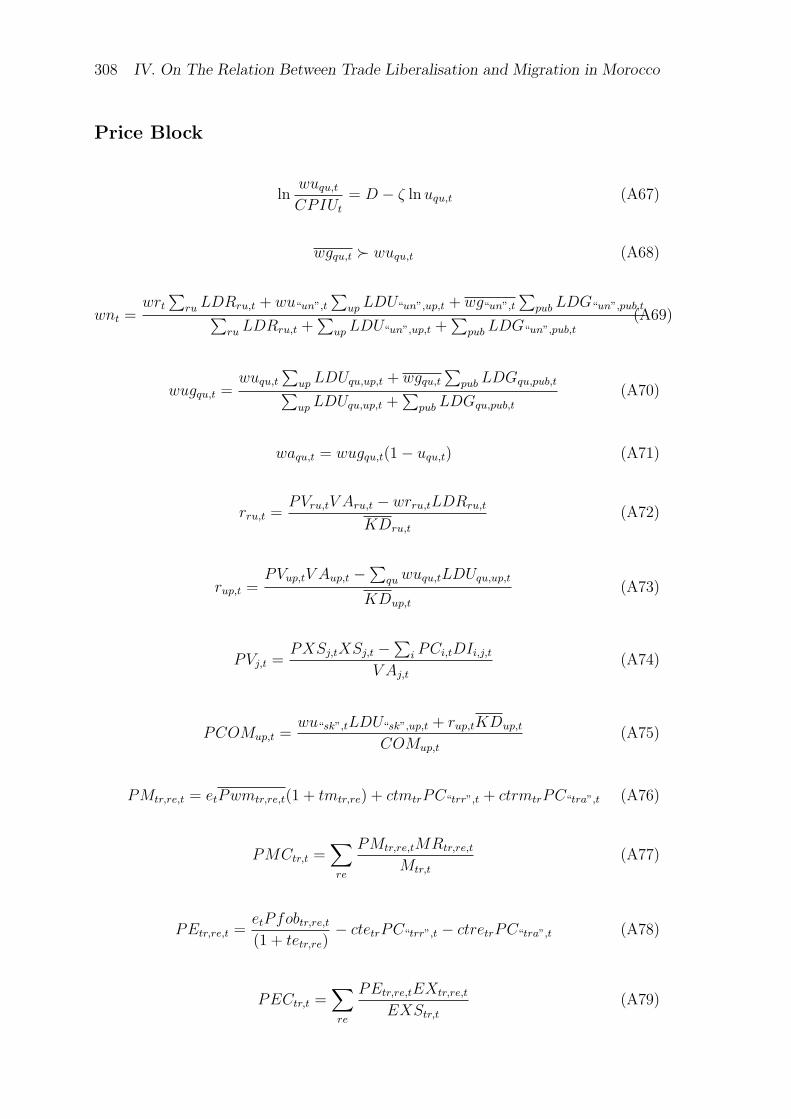
308 IV. On The Relation Between Trade Liberalisation and Migration in Morocco

Price Block

lnwuqu,tCPIUt

= D − ζ lnuqu,t (A67)

wgqu,t wuqu,t (A68)

wnt =wrt

∑ru LDRru,t + wu“un”,t

∑up LDU“un”,up,t + wg“un”,t

∑pub LDG“un”,pub,t∑

ru LDRru,t +∑

up LDU“un”,up,t +∑

pub LDG“un”,pub,t

(A69)

wugqu,t =wuqu,t

∑up LDUqu,up,t + wgqu,t

∑pub LDGqu,pub,t∑

up LDUqu,up,t +∑

pub LDGqu,pub,t

(A70)

waqu,t = wugqu,t(1− uqu,t) (A71)

rru,t =PVru,tV Aru,t − wrru,tLDRru,t

KDru,t

(A72)

rup,t =PVup,tV Aup,t −

∑quwuqu,tLDUqu,up,t

KDup,t

(A73)

PVj,t =PXSj,tXSj,t −

∑i PCi,tDIi,j,t

V Aj,t(A74)

PCOMup,t =wu“sk”,tLDU“sk”,up,t + rup,tKDup,t

COMup,t

(A75)

PMtr,re,t = etPwmtr,re,t(1 + tmtr,re) + ctmtrPC“trr”,t + ctrmtrPC“tra”,t (A76)

PMCtr,t =∑re

PMtr,re,tMRtr,re,t

Mtr,t

(A77)

PEtr,re,t =etPfobtr,re,t(1 + tetr,re)

− ctetrPC“trr”,t − ctretrPC“tra”,t (A78)

PECtr,t =∑re

PEtr,re,tEXtr,re,t

EXStr,t(A79)

309

PCtr,t = (1 + txtradjt)DOMtr,tPDtr,t +

∑reMRtr,re,tPMtr,re,t

Qtr,t

(A80)

PCntr,t = PDntr,t (A81)

PDj,t = PLj,t + ctdjPC“trr”,t + ctrdjPC“tra”,t (A82)

Ptr,t =PLtr,tDOMtr,t + PECtr,tEXStr,t

DDtr,t

(A83)

Pntr,t = PLntr,t (A84)

PXSj,t =∑i

Pi,tDSj,i,tXXSj,t

(A85)

PINVt =∏i

(PCi,tµi

)µi

(A86)

CPIt =∑i

θ1iPCi,t (A87)

CPIRt =∑i

θ2i,“hr”PCi,t (A88)

CPIUt =∑i

θ2i,“hu”PCi,t (A89)

Pindext =∑j

θjPVj,t (A90)

Dynamics

STKR1t+1 = STKR1t(1− χ1“un”) + EMRt (A91)

STKU1qu,t+1 = STKU1qu,t(1− χ1qu) + EMUqu,t (A92)

STKR2t+1 = STKR2t(1− χ2“un”) + χ1“un”STKR1t (A93)

310 IV. On The Relation Between Trade Liberalisation and Migration in Morocco

STKU2qu,t+1 = STKU2qu,t(1− χ2qu) + χ1quSTKU1qu,t (A94)

STKR3t+1 = STKR3t + χ2“un”STKR2t (A95)

STKU3qu,t+1 = STKU3qu,t + χ2quSTKU2qu,t (A96)

TSTKt = STKR1t + STKR2t + STKR3t + (A97)∑qu

(STKU1qu,t + STKU2qu,t + STKU3qu,t)

ISTKt+1 = ISTKt +MIGt (A98)

KDps,t+1 = (1− depps)KDps,t + INV Dps,t (A99)

INV Dps,t

KDps,t

= D1ps(rps,t

PINVt(depps + it))2 +

D2psrps,t

PINVt(depps + it)(A100)

V ARKDpub,t = KDpub,t −KDpub,t−1 (A101)

MCt = V3(TSTKt)ν (A102)

Gi,t+1 = Gi,t(1 + gG) (A103)

A1ps,t+1 = A1ps,t(1 + gA1) (A104)

LSRt+1 = LSRt(1 + gLSR)−MIGt − EMRt (A105)

LSU“un”,t+1 = LSU“un”,t(1 + gLSU)− skaLSU“sk”,t +

MIGt − EMU“un”,t (A106)

LSU“sk”,t+1 = LSU“sk”,t(1 + ska)− EMU“sk”,t (A107)

311

Equilibrium Conditions and Closure

NATRt =∑ru

LDRru,t (A108)

(NATU“un”,t + (1− imc)MIGt)(1− u“un”,t) =∑up

LDU“un”,up,t +∑pub

LDG“un”,pub,t (A109)

NATU“sk”,t(1− u“sk”,t) =∑up

LDU“sk”,up,t +∑pub

LDG“sk”,pub,t (A110)

Qi,t = Gi,t +DITi,t +∑h

CTi,h,t + INVi,t + STKi,t (A111)

Q“trr”,t = G“trr”,t +DIT“trr”,t +∑h

CT“trr”,h,t + INV“trr”,t +

STK“trr”,t +∑i

TMAi,t (A112)

Q“tra”,t = G“tra”,t +DIT“tra”,t +∑h

CT“tra”,h,t + INV“tra”,t +

STK“tra”,t +∑i

TRMi,t (A113)

EXStr,t = EXDtr,t (A114)

ITt +∑i

STKi,tPCi,t = etS”row”,t +∑da

Sda,t (A115)

CLOSEt = S“gv”,t/NGDPt (A116)

ITV OLt = SIt(∑ps

INV Dps,t + V ARKDt) (A117)

The Imperfect Competition Module

PDimc,t − V Cimc,tPDimc,t

=1

NBRimc,tPELASimc,t(A118)

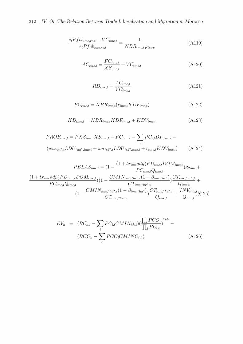
312 IV. On The Relation Between Trade Liberalisation and Migration in Morocco

etPfobimc,re,t − V Cimc,tetPfobimc,re,t

=1

NBRimc,tϕtr,re(A119)

ACimc,t =FCimc,tXSimc,t

+ V Cimc,t (A120)

RDimc,t =ACimc,tV Cimc,t

(A121)

FCimc,t = NBRimc,t(rimc,tKDFimc,t) (A122)

KDimc,t = NBRimc,tKDFimc,t +KDVimc,t (A123)

PROFimc,t = PXSimc,tXSimc,t − FCimc,t −∑i

PCi,tDIi,imc,t −

(wu“un”,tLDU“un”,imc,t + wu“sk”,tLDU“sk”,imc,t + rimc,tKDVimc,t) (A124)

PELASimc,t = (1− (1 + tximcadjt)PDimc,tDOMimc,t

PCimc,tQimc,t

)κ2imc +

(1 + tximcadjt)PDimc,tDOMimc,t

PCimc,tQimc,t

((1− CMINimc,“hr”,t(1− βimc,“hr”)

CTimc,“hr”,t)CTimc,“hr”,tQimc,t

+

(1− CMINimc,“hu”,t(1− βimc,“hu”)

CTimc,“hu”,t

)CTimc,“hu”,t

Qimc,t

+INVimc,tQimc,t

))(A125)

EVh = (BCh,t −∑i

PCi,tCMINi,h,t)(

∏i PCOi∏i PCi,t

)βi,h

−

(BCOh −∑i

PCOiCMINOi,h) (A126)

313

IV.D Appendix D: Tables

Table IV.2: The BAU Growth Path - Perfect CompetitionPercentage Change with Respect to the Base Year

t t+5 t+10 t+15Economic growthReal GDP at factor cost 0.00 11.48 31.51 59.15Real GNP 0.00 11.00 30.45 56.85Real wageRural 0.00 11.29 24.19 38.81Urban unskilled 0.00 0.99 6.00 16.97Urban skilled 0.00 2.93 10.35 43.23UnemploymentUnskilled 0.00 -9.34 -44.17 -79.14Skilled 0.00 -25.05 -62.65 -97.25Migration flowsRural 0.00 1.79 -2.64 -13.18Urban unskilled 0.00 21.06 19.86 2.91Urban skilled 0.00 3.08 -10.53 -30.91Internal 0.00 -18.10 -21.38 -17.05Household real disposable incomeRural 0.00 6.39 13.79 22.00Urban 0.00 9.41 26.84 52.80RemittancesTo rural household 0.00 1.47 -6.83 -23.77To urban household:From unskilled migrants 0.00 45.30 22.89 -31.52From skilled migrants 0.00 -34.99 -62.20 -79.59External tradeTotal export volume 0.00 12.31 38.61 77.43To the EU 0.00 11.61 36.03 71.54To the RoW 0.00 14.18 45.53 93.18Total import volume 0.00 8.60 26.90 54.96From the EU 0.00 8.39 26.51 54.47From the RoW 0.00 8.92 27.50 55.69Real exchange rate 0.00 4.24 6.41 6.77

Source: Author’s calculations.

314 IV. On The Relation Between Trade Liberalisation and Migration in Morocco

Table IV.3: The BAU Growth Path - Imperfect Competition (LR)Percentage Change with Respect to the Base Year

t t+5 t+10 t+15Economic growthReal GDP at factor cost 0.00 12.26 34.70 65.98Real GNP 0.00 10.73 29.28 55.60Real wageRural 0.00 9.96 22.17 37.48Urban unskilled 0.00 2.09 10.67 29.44Urban skilled 0.00 3.06 11.22 53.61UnemploymentUnskilled 0.00 -18.71 -63.71 -92.43Skilled 0.00 -26.01 -65.46 -98.63Migration flowsRural 0.00 -1.08 -11.27 -28.71Urban unskilled 0.00 12.43 -1.03 -23.77Urban skilled 0.00 -2.13 -21.53 -44.66Internal 0.00 -11.60 -5.90 -6.28Household real disposable incomeRural 0.00 6.11 13.13 20.72Urban 0.00 11.27 33.23 66.78RemittancesTo rural household 0.00 2.16 -6.78 -25.10To urban household:From unskilled migrants 0.00 32.81 -7.10 -58.81From skilled migrants 0.00 -37.76 -67.31 -84.62External tradeTotal export volume 0.00 14.73 48.93 99.20To the EU 0.00 13.53 44.01 87.56To the RoW 0.00 17.93 62.08 130.30Total import volume 0.00 11.58 37.14 76.61From the EU 0.00 11.55 37.33 77.33From the RoW 0.00 11.61 36.86 75.51Real exchange rate 0.00 2.06 1.59 -0.28

Source: Author’s calculations.

315

Table IV.4: The BAU Growth Path - Imperfect Competition (SR)Percentage Change with Respect to the Base Year

t t+5 t+10 t+15Economic growthReal GDP at factor cost 0.00 12.13 33.88 64.41Real GNP 0.00 10.65 28.67 54.19Real wageRural 0.00 9.77 21.95 37.32Urban unskilled 0.00 1.77 9.07 22.92Urban skilled 0.00 3.04 10.99 47.53UnemploymentUnskilled 0.00 -16.09 -58.02 -91.12Skilled 0.00 -25.86 -64.75 -97.69Migration flowsRural 0.00 -0.36 -8.86 -23.81Urban unskilled 0.00 14.31 4.51 -15.58Urban skilled 0.00 -1.15 -18.76 -40.54Internal 0.00 -12.52 -9.72 -1.20Household real disposable incomeRural 0.00 6.03 13.06 21.06Urban 0.00 10.99 31.76 63.35RemittancesTo rural household 0.00 2.60 -5.95 -24.63To urban household:From unskilled migrants 0.00 34.75 -0.89 -53.22From skilled migrants 0.00 -37.35 -66.23 -83.51External tradeTotal export volume 0.00 14.80 47.87 97.01To the EU 0.00 13.66 43.53 87.15To the RoW 0.00 17.85 59.46 123.38Total import volume 0.00 11.72 36.40 74.39From the EU 0.00 11.73 36.63 75.10From the RoW 0.00 11.72 36.07 73.30Real exchange rate 0.00 2.41 2.72 1.77

Source: Author’s calculations.

316 IV. On The Relation Between Trade Liberalisation and Migration in Morocco

Table IV.5: Economic growthPercentage Change with Respect to the BAU Growth Path

t t+5 t+10 t+15Gradual FTA - Perfect CompetitionReal GDP at factor cost 0.01 -0.05 -0.31 -0.66Real GNP -7.57 -7.04 -5.41 -3.27Gradual FTA - Imperfect Competition (LR)Real GDP at factor cost 0.05 0.09 -0.09 -0.43Real GNP -0.10 -0.03 -0.17 -0.42Gradual FTA - Imperfect Competition (SR)Real GDP at factor cost 0.04 0.13 0.06 -0.24Real GNP -0.10 -0.03 -0.10 -0.32Gradual MULTI - Perfect CompetitionReal GDP at factor cost 0.01 0.03 -0.04 -0.20Real GNP -7.70 -7.05 -5.26 -3.23Gradual MULTI - Imperfect Competition (LR)Real GDP at factor cost 0.09 0.35 0.52 0.44Real GNP -0.17 0.10 0.26 0.33Gradual MULTI - Imperfect Competition (SR)Real GDP at factor cost 0.08 0.45 0.87 1.01Real GNP -0.17 0.11 0.45 0.72Instantaneous FTA - Perfect CompetitionReal GDP at factor cost -0.02 -0.33 -0.73 -1.13Real GNP -8.37 -7.15 -5.62 -3.91Instantaneous FTA - Imperfect Competition (LR)Real GDP at factor cost 0.18 -0.14 -0.52 -0.81Real GNP -0.55 -0.08 -0.43 -0.75Instantaneous FTA - Imperfect Competition (SR)Real GDP at factor cost 0.16 -0.03 -0.27 -0.47Real GNP -0.55 -0.07 -0.30 -0.53Instantaneous MULTI - Perfect CompetitionReal GDP at factor cost -0.08 -0.19 -0.36 -0.55Real GNP -8.91 -7.08 -5.38 -3.50Instantaneous MULTI - Imperfect Competition (LR)Real GDP at factor cost 0.28 0.28 0.26 0.19Real GNP -0.82 0.19 0.16 0.09Instantaneous MULTI - Imperfect Competition (SR)Real GDP at factor cost 0.25 0.52 0.83 0.61Real GNP -0.81 0.26 0.49 0.40

Source: Author’s calculations.

317

Table IV.6: Real WagePercentage Change with Respect to the BAU Growth Path

t t+5 t+10 t+15Gradual FTA - Perfect CompetitionRural -0.77 -0.94 -1.28 1.00Urban unskilled 0.02 0.06 -0.09 -4.86Urban skilled 0.01 0.05 0.01 -0.20Gradual FTA - Imperfect Competition (LR)Rural -0.80 -0.88 -1.03 -0.16Urban unskilled 0.07 0.20 0.09 -0.46Urban skilled 0.02 0.06 0.02 -0.95Gradual FTA - Imperfect Competition (SR)Rural -0.76 -0.51 -0.39 0.24Urban unskilled 0.10 0.31 0.39 1.29Urban skilled 0.02 0.07 0.06 -0.56Gradual MULTI - Perfect CompetitionRural -1.18 -1.03 -1.24 -0.73Urban unskilled 0.01 0.16 0.23 0.34Urban skilled 0.01 0.10 0.17 0.54Gradual MULTI - Imperfect Competition (LR)Rural -1.33 -1.20 -1.19 0.07Urban unskilled 0.12 0.50 0.88 0.77Urban skilled 0.03 0.13 0.26 0.81Gradual MULTI - Imperfect Competition (SR)Rural -1.24 -0.58 -0.11 1.16Urban unskilled 0.18 0.75 1.55 3.19Urban skilled 0.03 0.15 0.35 3.07Instantaneous FTA - Perfect CompetitionRural -5.24 -0.65 -0.87 -1.08Urban unskilled -0.04 -0.16 -0.41 -0.87Urban skilled 0.01 0.02 -0.13 -1.37Instantaneous FTA - Imperfect Competition (LR)Rural -5.46 -0.43 -0.23 -0.10Urban unskilled 0.23 -0.05 -0.52 -1.13Urban skilled 0.05 0.02 -0.20 -2.06Instantaneous FTA - Imperfect Competition (SR)Rural -5.23 0.15 0.53 0.41Urban unskilled 0.37 0.12 -0.13 -0.47Urban skilled 0.05 0.03 -0.14 -1.07Instantaneous MULTI - Perfect CompetitionRural -6.39 -0.57 -0.72 -0.93Urban unskilled -0.20 -0.01 0.00 0.01Urban skilled 0.00 0.08 0.06 -0.05Instantaneous MULTI - Imperfect Competition (LR)Rural -7.36 -0.59 -0.11 0.28Urban unskilled 0.34 0.35 0.36 0.21Urban skilled 0.07 0.10 0.07 -0.07Instantaneous MULTI - Imperfect Competition (SR)Rural -6.97 0.36 1.25 1.64Urban unskilled 0.65 0.74 1.18 2.82Urban skilled 0.07 0.14 0.21 2.34

Source: Author’s calculations.

318 IV. On The Relation Between Trade Liberalisation and Migration in Morocco

Table IV.7: UnemploymentPercentage Change with Respect to the BAU Growth Path

t t+5 t+10 t+15Gradual FTA - Perfect CompetitionUnskilled -0.19 -0.61 0.89 3.87Skilled -0.08 -0.51 -0.15 3.50Gradual FTA - Imperfect Competition (LR)Unskilled -0.74 -1.98 -0.91 3.95Skilled -0.16 -0.64 -0.20 5.66Gradual FTA - Imperfect Competition (SR)Unskilled -1.00 -3.05 -3.84 -0.84Skilled -0.16 -0.68 -0.56 3.71Gradual MULTI - Perfect CompetitionUnskilled -0.07 -1.58 -2.28 -3.34Skilled -0.10 -0.95 -1.69 -5.20Gradual MULTI - Imperfect Competition (LR)Unskilled -1.23 -4.89 -8.40 -7.35Skilled -0.26 -1.31 -2.54 -7.76Gradual MULTI - Imperfect Competition (SR)Unskilled -1.83 -7.20 -14.26 -16.83Skilled -0.26 -1.44 -3.40 -9.52Instantaneous FTA - Perfect CompetitionUnskilled 0.45 1.58 4.19 9.08Skilled -0.09 -0.16 1.33 14.77Instantaneous FTA - Imperfect Competition (LR)Unskilled -2.26 0.53 5.38 12.04Skilled -0.48 -0.17 2.05 23.20Instantaneous FTA - Imperfect Competition (SR)Unskilled -3.67 -1.22 1.26 4.86Skilled -0.46 -0.32 1.45 11.36Instantaneous MULTI - Perfect CompetitionUnskilled 2.01 0.10 -0.03 -0.08Skilled 0.03 -0.78 -0.62 0.46Instantaneous MULTI - Imperfect Competition (LR)Unskilled -3.34 -3.47 -3.52 -2.04Skilled -0.71 -1.04 -0.74 0.66Instantaneous MULTI - Imperfect Competition (SR)Unskilled -6.23 -7.10 -11.05 -13.73Skilled -0.69 -1.40 -2.07 -4.81

Source: Author’s calculations.

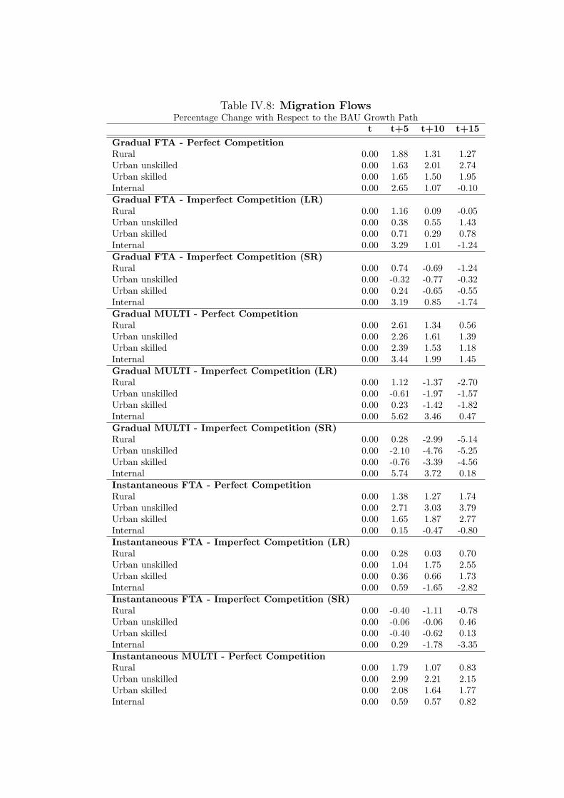
Table IV.8: Migration FlowsPercentage Change with Respect to the BAU Growth Path

t t+5 t+10 t+15Gradual FTA - Perfect CompetitionRural 0.00 1.88 1.31 1.27Urban unskilled 0.00 1.63 2.01 2.74Urban skilled 0.00 1.65 1.50 1.95Internal 0.00 2.65 1.07 -0.10Gradual FTA - Imperfect Competition (LR)Rural 0.00 1.16 0.09 -0.05Urban unskilled 0.00 0.38 0.55 1.43Urban skilled 0.00 0.71 0.29 0.78Internal 0.00 3.29 1.01 -1.24Gradual FTA - Imperfect Competition (SR)Rural 0.00 0.74 -0.69 -1.24Urban unskilled 0.00 -0.32 -0.77 -0.32Urban skilled 0.00 0.24 -0.65 -0.55Internal 0.00 3.19 0.85 -1.74Gradual MULTI - Perfect CompetitionRural 0.00 2.61 1.34 0.56Urban unskilled 0.00 2.26 1.61 1.39Urban skilled 0.00 2.39 1.53 1.18Internal 0.00 3.44 1.99 1.45Gradual MULTI - Imperfect Competition (LR)Rural 0.00 1.12 -1.37 -2.70Urban unskilled 0.00 -0.61 -1.97 -1.57Urban skilled 0.00 0.23 -1.42 -1.82Internal 0.00 5.62 3.46 0.47Gradual MULTI - Imperfect Competition (SR)Rural 0.00 0.28 -2.99 -5.14Urban unskilled 0.00 -2.10 -4.76 -5.25Urban skilled 0.00 -0.76 -3.39 -4.56Internal 0.00 5.74 3.72 0.18Instantaneous FTA - Perfect CompetitionRural 0.00 1.38 1.27 1.74Urban unskilled 0.00 2.71 3.03 3.79Urban skilled 0.00 1.65 1.87 2.77Internal 0.00 0.15 -0.47 -0.80Instantaneous FTA - Imperfect Competition (LR)Rural 0.00 0.28 0.03 0.70Urban unskilled 0.00 1.04 1.75 2.55Urban skilled 0.00 0.36 0.66 1.73Internal 0.00 0.59 -1.65 -2.82Instantaneous FTA - Imperfect Competition (SR)Rural 0.00 -0.40 -1.11 -0.78Urban unskilled 0.00 -0.06 -0.06 0.46Urban skilled 0.00 -0.40 -0.62 0.13Internal 0.00 0.29 -1.78 -3.35Instantaneous MULTI - Perfect CompetitionRural 0.00 1.79 1.07 0.83Urban unskilled 0.00 2.99 2.21 2.15Urban skilled 0.00 2.08 1.64 1.77Internal 0.00 0.59 0.57 0.82

Instantaneous MULTI - Imperfect Competition (LR)Rural 0.00 -0.52 -2.09 -2.41Urban unskilled 0.00 -0.89 -1.42 -0.85Urban skilled 0.00 -0.90 -1.59 -1.32Internal 0.00 2.93 0.66 -1.31Instantaneous MULTI - Imperfect Competition (SR)Rural 0.00 -1.88 -4.26 -5.33Urban unskilled 0.00 -3.25 -5.05 -5.08Urban skilled 0.00 -2.52 -4.18 -4.49Internal 0.00 3.02 0.91 -1.76

Source: Author’s calculations.

Table IV.9: Household Real Disposable IncomePercentage Change with Respect to the BAU Growth Path

t t+5 t+10 t+15Gradual FTA - Perfect CompetitionRural -0.20 -0.17 -0.37 -0.38Urban 0.12 0.18 -0.01 -0.17Gradual FTA - Imperfect Competition (LR)Rural -0.20 -0.04 -0.29 -0.11Urban 0.14 0.40 0.14 -0.27Gradual FTA - Imperfect Competition (SR)Rural -0.18 -0.00 -0.03 -0.04Urban 0.10 0.41 0.31 -0.40Gradual MULTI - Perfect CompetitionRural -0.32 -0.11 -0.24 -0.26Urban 0.19 0.36 0.31 0.40Gradual MULTI - Imperfect Competition (LR)Rural -0.32 -0.14 -0.29 0.05Urban 0.24 0.86 1.07 1.06Gradual MULTI - Imperfect Competition (SR)Rural -0.29 -0.09 -0.15 0.40Urban 0.16 0.99 1.52 1.34Instantaneous FTA - Perfect CompetitionRural -1.50 -0.07 -0.31 -0.59Urban -0.81 -0.82 -0.50 -0.96Instantaneous FTA - Imperfect Competition (LR)Rural -1.48 -0.02 -0.11 -0.10Urban 0.00 -0.08 -0.50 -1.00Instantaneous FTA - Imperfect Competition (SR)Rural -1.39 0.20 0.20 0.10Urban 0.08 0.19 -0.22 -1.03Instantaneous MULTI - Perfect CompetitionRural -1.85 -0.10 -0.14 -0.45Urban 0.96 0.20 0.05 -0.06Instantaneous MULTI - Imperfect Competition (LR)Rural -1.96 -0.04 -0.05 -0.09Urban 1.23 0.77 0.64 0.52Instantaneous MULTI - Imperfect Competition (SR)Rural -1.81 0.39 0.48 0.56Urban 0.82 1.06 1.29 0.99

Source: Author’s calculations.

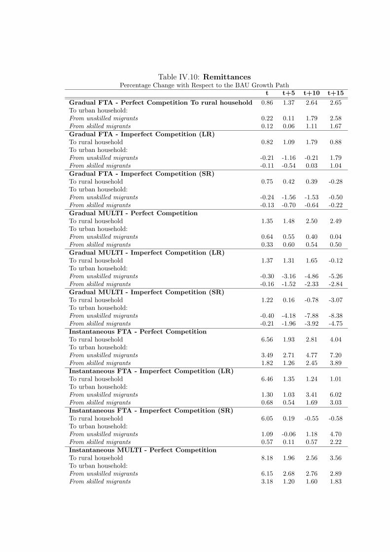
Table IV.10: RemittancesPercentage Change with Respect to the BAU Growth Path

t t+5 t+10 t+15Gradual FTA - Perfect Competition To rural household 0.86 1.37 2.64 2.65To urban household:From unskilled migrants 0.22 0.11 1.79 2.58From skilled migrants 0.12 0.06 1.11 1.67Gradual FTA - Imperfect Competition (LR)To rural household 0.82 1.09 1.79 0.88To urban household:From unskilled migrants -0.21 -1.16 -0.21 1.79From skilled migrants -0.11 -0.54 0.03 1.04Gradual FTA - Imperfect Competition (SR)To rural household 0.75 0.42 0.39 -0.28To urban household:From unskilled migrants -0.24 -1.56 -1.53 -0.50From skilled migrants -0.13 -0.70 -0.64 -0.22Gradual MULTI - Perfect CompetitionTo rural household 1.35 1.48 2.50 2.49To urban household:From unskilled migrants 0.64 0.55 0.40 0.04From skilled migrants 0.33 0.60 0.54 0.50Gradual MULTI - Imperfect Competition (LR)To rural household 1.37 1.31 1.65 -0.12To urban household:From unskilled migrants -0.30 -3.16 -4.86 -5.26From skilled migrants -0.16 -1.52 -2.33 -2.84Gradual MULTI - Imperfect Competition (SR)To rural household 1.22 0.16 -0.78 -3.07To urban household:From unskilled migrants -0.40 -4.18 -7.88 -8.38From skilled migrants -0.21 -1.96 -3.92 -4.75Instantaneous FTA - Perfect CompetitionTo rural household 6.56 1.93 2.81 4.04To urban household:From unskilled migrants 3.49 2.71 4.77 7.20From skilled migrants 1.82 1.26 2.45 3.89Instantaneous FTA - Imperfect Competition (LR)To rural household 6.46 1.35 1.24 1.01To urban household:From unskilled migrants 1.30 1.03 3.41 6.02From skilled migrants 0.68 0.54 1.69 3.03Instantaneous FTA - Imperfect Competition (SR)To rural household 6.05 0.19 -0.55 -0.58To urban household:From unskilled migrants 1.09 -0.06 1.18 4.70From skilled migrants 0.57 0.11 0.57 2.22Instantaneous MULTI - Perfect CompetitionTo rural household 8.18 1.96 2.56 3.56To urban household:From unskilled migrants 6.15 2.68 2.76 2.89From skilled migrants 3.18 1.20 1.60 1.83

Instantaneous MULTI - Imperfect Competition (LR)To rural household 8.69 1.46 0.66 -0.44To urban household:From unskilled migrants 1.72 -1.91 -2.70 -2.64From skilled migrants 0.89 -0.86 -1.39 -1.71Instantaneous MULTI - Imperfect Competition (SR)To rural household 7.96 -0.47 -2.56 -4.28To urban household:From unskilled migrants 1.13 -4.34 -7.38 -7.30From skilled migrants 0.59 -1.87 -3.82 -4.45

Source: Author’s calculations.

Table IV.11: External TradePercentage Change with Respect to the BAU Growth Path

t t+5 t+10 t+15Gradual FTA - Perfect CompetitionTotal export volume 0.88 3.19 4.07 4.68To the EU 0.92 3.50 4.66 5.31To the RoW 0.76 2.39 2.61 3.20Total import volume 0.17 2.66 3.84 3.69From the EU 2.03 9.03 12.43 12.01From the RoW -2.64 -6.94 -9.08 -8.82Real exchange rate 0.94 0.87 1.18 0.71Gradual FTA - Imperfect Competition (LR)Total export volume 1.01 3.82 4.91 3.95To the EU 1.04 4.15 5.70 4.88To the RoW 0.95 2.98 3.04 1.93Total import volume 0.37 3.15 4.51 4.01From the EU 2.25 9.47 12.87 11.97From the RoW -2.46 -6.41 -8.19 -8.16Real exchange rate 0.72 0.48 0.55 0.16Gradual FTA - Imperfect Competition (SR)Total export volume 0.97 3.75 5.06 3.61To the EU 1.00 4.07 5.89 4.73To the RoW 0.91 2.93 3.06 1.11Total import volume 0.36 3.00 4.49 3.74From the EU 2.23 9.29 12.84 11.72From the RoW -2.48 -6.53 -8.21 -8.47Real exchange rate 0.67 0.38 0.31 -0.14Gradual MULTI - Perfect CompetitionTotal export volume 1.55 5.52 7.52 7.01To the EU 1.63 6.02 8.45 8.17To the RoW 1.36 4.24 5.22 4.24Total import volume 0.31 4.51 6.82 7.17From the EU -1.38 -1.21 -1.18 -0.86From the RoW 2.88 13.14 18.84 19.23Real exchange rate 1.63 1.29 1.55 0.81Gradual MULTI - Imperfect Competition (LR)Total export volume 1.85 7.04 9.86 9.42To the EU 1.91 7.72 11.61 12.05To the RoW 1.69 5.30 5.70 3.69Total import volume 0.76 5.84 9.01 9.38From the EU -0.91 0.09 0.89 1.15From the RoW 3.29 14.54 21.37 21.98Real exchange rate 1.17 0.39 0.17 -0.47Gradual MULTI - Imperfect Competition (SR)Total export volume 1.75 6.94 10.29 9.58To the EU 1.81 7.62 12.14 12.48To the RoW 1.60 5.19 5.83 3.08Total import volume 0.71 5.57 9.10 9.47From the EU -0.96 -0.17 0.96 1.19From the RoW 3.24 14.25 21.48 22.15Real exchange rate 1.05 0.15 -0.36 -1.14

Instantaneous FTA - Perfect CompetitionTotal export volume 4.99 4.36 3.38 2.52To the EU 5.27 4.94 4.09 3.28To the RoW 4.25 2.84 1.59 0.72Total import volume 1.31 4.37 3.78 2.97From the EU 9.55 13.28 12.46 11.30From the RoW -11.17 -9.06 -9.26 -9.55Real exchange rate 5.50 0.67 0.63 0.78Instantaneous FTA - Imperfect Competition (LR)Total export volume 5.72 5.33 4.28 3.26To the EU 5.94 6.17 5.55 4.52To the RoW 5.13 3.16 1.27 0.53Total import volume 2.35 5.05 4.35 3.38From the EU 10.70 13.93 12.81 11.32From the RoW -10.30 -8.40 -8.52 -8.78Real exchange rate 4.38 0.13 0.01 0.16Instantaneous FTA - Imperfect Competition (SR)Total export volume 5.48 5.39 4.67 3.11To the EU 5.70 6.24 6.06 4.65To the RoW 4.91 3.20 1.34 -0.34Total import volume 2.24 4.88 4.49 3.27From the EU 10.58 13.72 12.97 11.26From the RoW -10.38 -8.50 -8.41 -8.97Real exchange rate 4.07 -0.02 -0.30 -0.22Instantaneous MULTI - Perfect CompetitionTotal export volume 7.62 7.65 7.13 6.54To the EU 8.02 8.52 8.25 7.82To the RoW 6.57 5.36 4.34 3.51Total import volume 1.85 7.22 7.17 6.83From the EU -5.91 -0.72 -0.81 -1.15From the RoW 13.61 19.21 19.16 18.84Real exchange rate 8.32 0.98 0.79 0.82Instantaneous MULTI - Imperfect Competition (LR)Total export volume 9.01 10.09 9.91 9.24To the EU 9.37 11.59 12.47 12.52To the RoW 8.05 6.26 3.82 2.09Total import volume 3.96 9.22 9.54 9.22From the EU -3.82 1.16 1.38 0.98From the RoW 15.74 21.42 21.95 21.83Real exchange rate 6.01 -0.24 -0.61 -0.57Instantaneous MULTI - Imperfect Competition (SR)Total export volume 8.52 10.29 10.88 9.78To the EU 8.88 11.83 13.67 13.45To the RoW 7.55 6.33 4.14 1.55Total import volume 3.71 8.99 10.00 9.64From the EU -4.03 0.97 1.80 1.32From the RoW 15.42 21.15 22.48 22.37Real exchange rate 5.42 -0.60 -1.26 -1.35

Source: Author’s calculations.

Table IV.12: GDP at Factor CostFor Selected Values of Skilled Externality Parameter ske

Percentage Change with Respect to the BAU Growth Pathske Model Scenario t t+5 t+10 t+150.20 Imperfect Competition (LR) FTA 0.05 0.09 -0.09 -0.43

MULTI 0.09 0.35 0.51 0.48Imperfect Competition (SR) FTA 0.04 0.13 0.06 -0.19

MULTI 0.08 0.45 0.87 1.030.05 Imperfect Competition (LR) FTA 0.05 0.09 -0.09 -0.43

MULTI 0.09 0.35 0.52 0.44Imperfect Competition (SR) FTA 0.04 0.13 0.06 -0.19

MULTI 0.08 0.44 0.87 1.03Notes: FTA and MULTI stand here for gradual free trade agreement and gradual multilateralliberalisation.Source: Author’s calculations.

Table IV.13: GDP at Factor CostFor Selected Values of Base Year Profits

Percentage Change with Respect to the BAU Growth PathProfits Model Scenario t t+5 t+10 t+15

0 Imperfect Competition (LR)∗ FTA 0.06 0.10 -0.08 -0.43MULTI 0.10 0.37 0.53 0.44

Imperfect Competition (SR) FTA 0.05 0.13 0.06 -0.19MULTI 0.09 0.45 0.85 1.00

20% of capital Imperfect Competition (LR)∗ FTA 0.05 0.09 -0.08 -0.42remuneration MULTI 0.08 0.34 0.52 0.46

Imperfect Competition (SR) FTA 0.04 0.13 0.06 -0.55MULTI 0.07 0.45 0.90 0.69

10% of capital Imperfect Competition (LR)∗∗ FTA 0.05 0.10 -0.08 -0.36remuneration MULTI 0.09 0.36 0.53 0.47

Notes: (1) FTA and MULTI stand here for gradual free trade agreement and gradual multilateralliberalisation.(2) *: In the LR simulation, profits are brought back to their benchmark value.(3) **: Profits are brought back to zero.Source: Author’s calculations.

Table IV.14: GDP at Factor Cost - Imperfect CompetitionFor Selected Combinations of Remittance Elasticities

Percentage Change with Respect to the BAU Growth Pathγ1”un”,h γ1”sk”,h Model Scenario t t+5 t+10 t+15

-8.4 -2.2 LR FTA 0.05 0.10 -0.08 -0.44MULTI 0.09 0.36 0.52 0.43

SR FTA 0.05 0.13 0.06 -0.59MULTI 0.08 0.45 0.88 0.64

-8.4 -1.1 LR FTA 0.05 0.10 -0.08 -0.44MULTI 0.09 0.36 0.52 0.44

SR FTA 0.05 0.13 0.06 -0.59MULTI 0.08 0.45 0.88 0.65

-8.4 -4.2 LR FTA 0.05 0.10 -0.09 -0.45MULTI 0.09 0.35 0.52 0.43

SR FTA 0.05 0.13 0.06 -0.60MULTI 0.08 0.44 0.88 0.63

-4.2 -1.1 LR FTA 0.05 0.09 -0.09 -0.43MULTI 0.09 0.35 0.52 0.44

SR FTA 0.05 0.13 0.06 -0.54MULTI 0.08 0.45 0.87 0.67

Notes: (1) γ1”un”,h: Elasticity of international remittance rate by unskilled workerswith respect to household h’s real income.(2) γ1”sk”,h: Elasticity of international remittance rate by skilled workers withrespect to household h’s real income.Source: Author’s calculations.

Table IV.15: Remittances - Imperfect CompetitionFor Selected Combinations of Remittance Elasticities

Percentage Change with Respect to the BAU Growth Pathγ1”un”,h γ1”sk”,h Model Scenario Household t t+5 t+10 t+15

-8.4 -2.2 LR FTA Rural 1.17 1.39 2.59 1.32UrbanFrom unskilled migrants -0.49 -2.53 -0.61 3.79From skilled migrants -0.13 -0.50 0.07 1.25

MULTI Rural 1.95 1.67 2.51 -0.04UrbanFrom unskilled migrants -0.73 -6.25 -9.12 -8.91From skilled migrants -0.19 -1.43 -2.39 -2.74

SR FTA Rural 1.06 0.43 0.42 -0.36UrbanFrom unskilled migrants -0.54 -3.04 -2.76 -4.08From skilled migrants -0.14 -0.65 -0.65 -0.93

MULTI Rural 1.73 0.01 -1.19 -4.61UrbanFrom unskilled migrants -0.88 -7.64 -14.01 -13.19From skilled migrants -0.23 -1.83 -4.09 -4.77

-8.4 -1.1 LR FTA Rural 1.17 1.39 2.60 1.34UrbanFrom unskilled migrants -0.51 -2.60 -0.66 3.69From skilled migrants -0.07 -0.13 0.19 0.83

MULTI Rural 1.95 1.67 2.51 -0.05UrbanFrom unskilled migrants -0.75 -6.38 -9.23 -9.02From skilled migrants -0.10 -0.57 -1.25 -1.69

SR FTA Rural 1.06 0.43 0.44 -0.36UrbanFrom unskilled migrants -0.56 -3.11 -2.82 -3.96From skilled migrants -0.07 -0.24 -0.33 -0.33

MULTI Rural 1.73 0.01 -1.19 -4.62UrbanFrom unskilled migrants -0.91 -7.79 -14.13 -13.29From skilled migrants -0.12 -0.85 -2.45 -3.42

-8.4 -4.2 LR FTA Rural 1.17 1.39 2.58 1.32UrbanFrom unskilled migrants -0.46 -2.45 -0.55 3.92From skilled migrants -0.23 -1.15 -0.13 2.06

MULTI Rural 1.95 1.67 2.51 -0.05UrbanFrom unskilled migrants -0.68 -6.07 -9.02 -8.81From skilled migrants -0.34 -2.92 -4.39 -4.59

SR FTA Rural 1.06 0.42 0.41 -0.34UrbanFrom unskilled migrants -0.50 -2.95 -2.71 -4.24From skilled migrants -0.25 -1.36 -1.21 -2.07

MULTI Rural 1.73 0.01 -1.20 -4.60UrbanFrom unskilled migrants -0.82 -7.43 -13.91 -13.11From skilled migrants -0.41 -3.53 -6.98 -7.16

Notes: (1) γ1”un”,h: Elasticity of international remittance rate by unskilled workers with respect to household h’sreal income.(2) γ1”sk”,h: Elasticity of international remittance rate by skilled workers with respect to household h’s realincome.(3) FTA and MULTI stand here for gradual free trade agreement and gradual multilateral liberalisation.Source: Author’s calculations.

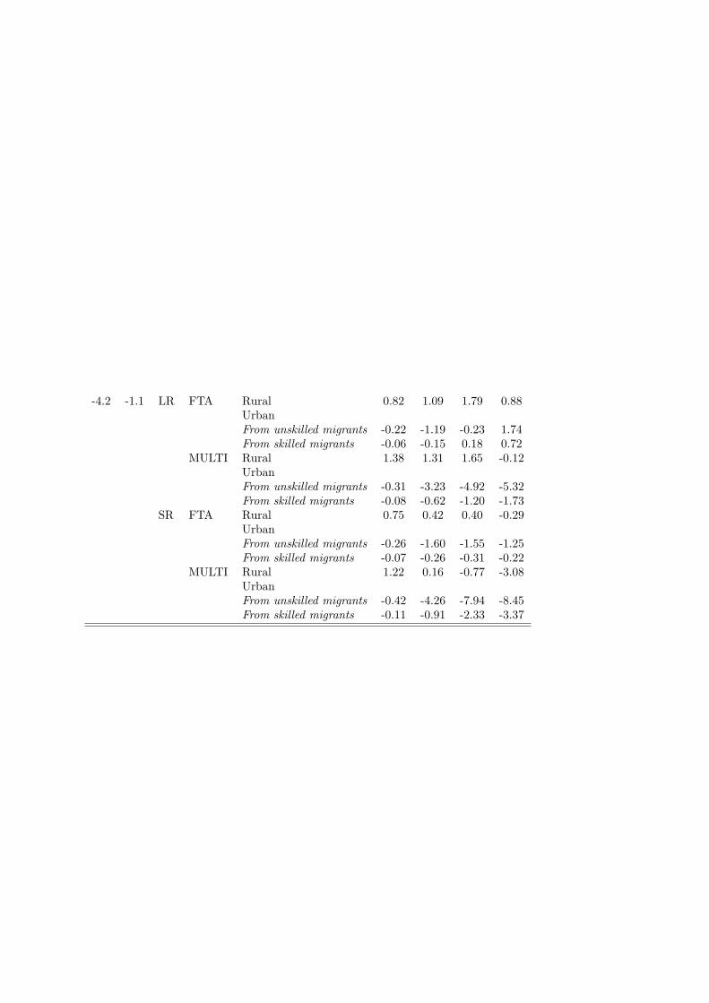
-4.2 -1.1 LR FTA Rural 0.82 1.09 1.79 0.88UrbanFrom unskilled migrants -0.22 -1.19 -0.23 1.74From skilled migrants -0.06 -0.15 0.18 0.72

MULTI Rural 1.38 1.31 1.65 -0.12UrbanFrom unskilled migrants -0.31 -3.23 -4.92 -5.32From skilled migrants -0.08 -0.62 -1.20 -1.73

SR FTA Rural 0.75 0.42 0.40 -0.29UrbanFrom unskilled migrants -0.26 -1.60 -1.55 -1.25From skilled migrants -0.07 -0.26 -0.31 -0.22

MULTI Rural 1.22 0.16 -0.77 -3.08UrbanFrom unskilled migrants -0.42 -4.26 -7.94 -8.45From skilled migrants -0.11 -0.91 -2.33 -3.37

Table IV.16: Household Real Disposable Income - Imperfect CompetitionFor Selected Combinations of Remittance Elasticities

Percentage Change with Respect to the BAU Growth Pathγ1”un”,h γ1”sk”,h Model Scenario Household t t+5 t+10 t+15

-8.4 -2.2 LR FTA Rural -0.14 -0.11 -0.24 -0.11Urban 0.06 0.35 0.11 -0.37

MULTI Rural -0.23 -0.11 -0.25 0.05Urban 0.09 0.81 1.07 1.00

SR FTA Rural -0.13 0.00 -0.02 -0.03Urban 0.06 0.39 0.30 -0.52

MULTI Rural -0.20 -0.06 -0.12 0.38Urban 0.10 0.93 1.57 1.30

-8.4 -1.1 LR FTA Rural -0.14 -0.11 -0.24 -0.11Urban 0.06 0.36 0.12 -0.36

MULTI Rural -0.23 -0.11 -0.25 0.05Urban 0.09 0.83 1.09 1.01

SR FTA Rural -0.13 0.00 -0.02 -0.03Urban 0.07 0.39 0.31 -0.51

MULTI Rural -0.20 -0.06 -0.12 0.39Urban 0.11 0.95 1.59 1.31

-8.4 -4.2 LR FTA Rural -0.14 -0.11 -0.24 -0.11Urban 0.05 0.34 0.11 -0.38

MULTI Rural -0.23 -0.11 -0.25 0.05Urban 0.08 0.79 1.06 0.98

SR FTA Rural -0.13 0.00 -0.02 -0.02Urban 0.06 0.38 0.29 -0.54

MULTI Rural -0.20 -0.06 -0.12 0.38Urban 0.10 0.91 1.56 1.29

-4.2 -1.1 LR FTA Rural -0.20 -0.14 -0.29 -0.11Urban 0.05 0.38 0.14 -0.26

MULTI Rural -0.32 -0.14 -0.29 0.05Urban 0.07 0.87 1.08 1.07

SR FTA Rural -0.18 0.00 -0.03 -0.04Urban 0.06 0.42 0.31 -0.38

MULTI Rural -0.29 -0.09 -0.15 0.41Urban 0.10 1.01 1.53 1.36

Notes: (1) γ1”un”,h: Elasticity of international remittance rate by unskilled workers with respect tohousehold h’s real income.(2) γ1”sk”,h: Elasticity of international remittance rate by skilled workers with respect to householdh’s real income.(3) FTA and MULTI stand here for gradual free trade agreement and gradual multilateral liberalisa-tion.Source: Author’s calculations.

General Conclusion

After the large interest in the impact of South-North migration on developed

countries, economists were particularly busy for years in looking at its effects

on developing countries. Undoubtedly, South-North migration is quantitatively

important. But as much tremendous as South-North migration is South-South

migration, accounting for 47% of total emigration from the South. In the real world,

the common case is a developing country having both the status of emigration and

immigration countries. This is for example the case of North African countries such

as Mauritania, Algeria, Libya, Morocco and Tunisia. They send migrants to the EU

and receive, in turn, immigrants from Sub-Saharan Africa (Senegal, Gambia, Sierra

Leone, Liberia, Mali and others) for transit or for stay. This is also true for many

other developing countries. The coexistence of inflows and outflows of workers raises

doubts about the effects of South-North migration on developing countries, especially

when they concern its impact on labour market. Indeed, if emigration helps raise

wages or diminish unemployment in the sending country, immigration acts in the

opposite direction. Besides, an interesting interdependency arises between inflows

and outflows of workers. On the one hand, if the labour market is taken into account

in the emigration decision, the pressure exerted by South-South migration on wages

and unemployment in the developing country may motivate people to leave. On the

other hand, the alleviating effect of South-North emigration on the labour market in

the sending country is able to attract immigration from another developing country.

What would be the overall impact of inflows and outflows of workers on the labour

market of the developing country?

331

332 General Conclusion

***

With respect to the literature on “Migration and Development”, this thesis

proposes to look over the scope of South-North migration. It gives a particular

attention to inflows and outflows of workers affecting a developing country. If South-

North migration helps raise wages or diminish unemployment in the sending region,

the conditions of the labour market make this region attractive for immigrants or for

internal migrants inside the country. Indeed, internal migration from disadvantaged

regions has been largely documented in the literature. Furthermore, immigration

and internal migration increase the pressure on the labour market of the receiving

region, stimulating outflows of workers from this region. This interdependency

between inflows and outflows of workers has been omitted in the literature on

the impact of emigration on labour market in the sending country. That is why

the literature argues that emigration reduces unemployment and/or increases the

wage rate. However, when inflows and outflows of workers coexist, the overall

impact of all migratory flows on domestic labour market is ambiguous. It depends

on the magnitude of inflows and outflows: if outflows are higher, unemployment

decreases, as it is found in the migration literature. By contrast, if inflows are

greater, unemployment increases.

The answer to this question is brought in the second chapter of this thesis.

Morocco is the country of application. It is the typical example of a developing

country undergoing the combination of inflows and outflows of workers. Chapter

2 proposes a modelling of all migration flows affecting the Moroccan urban labour

market: rural and urban emigration, internal migration from rural to urban areas,

and Sub-Saharan immigration to Moroccan urban areas. Migration flows depend

on the wage differential between the sending and receiving regions net of migration

costs. Therefore, this is a general equilibrium problem and to deal with, the analysis

is done with a static CGE model. Only African immigration does not depend on

wage differentials because it mainly occurs for security and personal reasons. Thus,

General Conclusion 333

the stock of African immigrants is exogenised and is subject to a shock reflecting

higher African immigration. The increase of international and internal migration is

simulated by a drop of internal and international migration costs. The results show

that the pressure of immigration and internal migration on Moroccan urban labour

market outweighs the alleviating effect of urban emigration, so that unemployment

rates by professional category increase. This result is contradictory to the literature

and suggests that the impact of migration on labour market should be apprehended

cautiously, by taking into consideration the characteristics of migratory flows in the

corresponding country.

The second question is related to the investment of remittances in developing

countries. Case studies argue that they are mainly invested in real estate, that is

called a “refugee sector”. The problem of the real estate activity is that construction

services are offered domestically and do not compete with exports. Therefore,

they do not profit from total factor productivity improvement, for example through

technology transfer in order to meet the world market quality standards. A sketchy

analysis suggests that the investment of remittances in productive exportable sectors

should create the conditions of a sustainable growth. This problem is dealt with in

a dynamic CGE model that shows the transmission channels by which remittances

affect households and sectors as well as the interactions between economic agents. In

contrast to the literature that is interested in the household impact of remittances,

this thesis proposes a overall view of the economy. To begin with, remittances

affect household income. But since a fraction of remittances is invested, they also

affect production and the demand for factors. In turn, wage variation modifies

household income. Besides, remittances affect the BoP and induce an appreciation

or a depreciation of the real exchange rate. Since the evolution of the exchange

rate enters in migration decision by changing the value of foreign wage in domestic

currency, it affects migration flows and thus the amount remitted. In order to

investigate the specific investment of remittances in real estate, a segmentation of

the savings markets is necessary where different savings sources finance investment

334 General Conclusion

in different sectors.

The answer to this question is given in Chapter 3. This chapter proposes a

dynamic CGE model applied to Morocco, with each source of savings being devoted

to investment in specific sectors. The application to Morocco is interesting especially

since it is the fourth developing country and the first MENA country in terms of

remittances received. Besides, 80% of remittances invested finance the real estate

sector. A 50% drop of the amount of remittances invested in the real estate sector is

then simulated. The results show that the investment of remittances in productive

sectors unexpectedly reduces the overall economic activity. This is due to the fact

that the real estate sector is highly integrated in the economy. It consumes an

important volume of intermediary inputs from the other sectors. Therefore, when

the real estate sector contracts after receiving less investment, the other sectors also

shrink because of a negative demand effect. Positive effects in terms of welfare and

economic growth only stem from government ability to attract investors through an

improvement in the country risk premium, and private efforts to reduce international

transfer costs. Indeed, with a better investment climate, foreign and domestic

investors have greater confidence in investment. Given that other things are equal,

the capital used in the production of all sectors rises and the production follows,

ceteris paribus, the evolution of the capital volume. This is translated in a higher

economic growth. Similarly, when transfer costs decrease, households receive a larger

value of remittances that increases their income, consumption budget and welfare.

Furthermore, as long as a fraction of remittances is invested, the drop in transfer

costs should, ceteris paribus, boost domestic investment in all sectors, and mostly

in real estate, enhancing economic growth.

The third question in which this thesis is interested concerns the labour market

effects of trade liberalisation for unskilled and skilled workers, and their indirect

effects on migration incentives. The relation between tariff removal and unskilled

and skilled migration is largely investigated on the theoretical ground, beginning

by the HO model. In an unskilled-labour abundant country that is advantaged in

General Conclusion 335

unskilled-labour intensive sectors, trade liberalisation should raise unskilled-labour

intensive exports as well as unskilled labour demand. Unskilled wage then increases,

reducing migration incentives. The opposite is true for skilled labour. But some

complications of this model are sufficient to reverse the results. Therefore, empirical

country-specific works must be done. The analysis is conducted with a dynamic

CGE model because trade agreements involve substantial changes in prices, resource

allocation and income, and affect capital stock through savings as well as human

capital and technology. Based on a robust and widely accepted modelling of agents’

behaviour, CGE models are able to provide a detailed description of the impact of

such shocks on the economy.

The CGE model is calibrated on the newest Moroccan SAM for the year 2003.

The country is in the bulk of the trade liberalisation process. It is about to achieve

a free trade area with the EU and has signed FTAs with the US, Turkey and other

Arab countries. The application to Morocco also allows to compare the results

with previous works on migration and trade liberalisation in Morocco, and to show

how some complications of the model are likely to reverse the results. Morocco is

unskilled-labour abundant and is advantaged in unskilled-labour intensive sectors.

Therefore, trade liberalisation should be a substitute for unskilled migration, and

a complement for skilled migration. However, the results show that the final effect

on labour demand also depends on the initial protection structure. Indeed, some

unskilled-intensive sectors, initially highly protected, shrink after tariff removal.

This is for example the case of agriculture. Rural unskilled labour demand then

decreases and the rural wage falls in order to balance the market. Unskilled rural

migration is thus stimulated. In urban areas, both skilled and unskilled labour

demand increase in the short run as well as wages. Skilled labour demand increases

in the short run because skilled-intensive sectors expand, selling more on foreign

markets thanks to the real exchange rate depreciation and to cheaper intermediary

inputs. Skilled and unskilled demand however decrease in the long run with increased

foreign competition, and so do wages. Despite falling unemployment in the short

336 General Conclusion

run, unskilled and skilled urban people choose to migrate, motivated by the exchange

rate depreciation that increases the value of the foreign wage in domestic currency.

In other words, there is a pull factor for urban emigration. When the FTA shock

is run with an imperfect competition framework, migration flows of skilled and

unskilled workers decrease, even in rural areas in the long run. Indeed, with

imperfect competition, the pro-competitive effect of trade liberalisation allows a

greater expansion of the economic activity, and thus a greater labour demand that

reduces unemployment and increases wages. Gradual multilateral liberalisation

strengthens the previous effects. The economic growth is even higher than the FTA

case because of cheaper inputs and greater real exchange rate depreciation that

improves export competitiveness on foreign markets. In the imperfect competition

model, all emigration flows decrease, more than the FTA shock, meaning that trade

liberalisation and migration are substitutes. In other words, the more the economy

grows, the lower are migration flows. The results of this chapter are contradictory

with the works of Bouzahzah et al. (2007) and Cogneau and Tapinos (1995) on

Morocco where migration is motivated by push factors due to tariff removal. In this

model, migration is mostly due to pull factors and may even decrease. This does

not mean that the previous works are wrong, but it puts forward the importance of

the conceptualised model, especially when some complications are likely to reverse

the results.

It is worth mentioning that the three above-mentioned CGE models are built on

the basis of Chapter 1 that presents a useful exercise to examine the functioning

of such models. The first chapter is an attempt to determine the appropriate

CGE framework adapted to use. It investigates how the results of a trade

liberalisation shock change under different structures of CGE models. It discusses

how trade liberalisation outcomes are affected by the change of the functional

forms corresponding to production (CES vs. Leontief), value added (CES vs.

Cobb Douglas), intermediary consumption (CES vs. Leontief), investment (CES

vs. Cobb-Douglas) and utility (Stone-Geary vs. Cobb-Douglas), as well as the

General Conclusion 337

choice of the numeraire, the macroeconomic closure (investment-driven vs. savings-

driven), the structure of the commodity market (imperfect vs. perfect competition)

and the time dimension (dynamic vs. static). The results are not considerably

affected when the functional forms are modified: only the classification of winners

and losers is altered as well as the magnitude of variable changes. They are, however,

more sensitive to changes of the intermediate consumption Leontief function, the

macroeconomic closure, the commodity market structure and the time horizon

adopted. Many changes are detected in signs. The importance of the imperfect

vs. perfect commodity market structure is felt in the last chapter of this thesis,

with imperfect competition leading to somewhat opposite results when compared to

those of perfect competition.

***

In economics as well as other model-based sciences, a modeller has to do a

sensitivity analysis to show the validity of the results generated from his numerical

model simulations. Indeed, results from simulation models are dependent on values

chosen for critical parameters such as elasticities or time preference parameters. A

sensitivity analysis is the study of how the output of a model varies, qualitatively

or quantitatively, following different sources of variation in input parameters. In

this thesis, a sensitivity analysis followed each chapter. The results come out to be

sufficiently robust to reasonable variation or combined variation of key parameters.

Some selected results of the sensitivity analysis are summarised in tables at the end

of each chapter and pointed out to in the analysis.

***

What is behind the scope of this thesis? The present work tackles some

interesting issues on “Migration and Development”. However, other aspects merit to

338 General Conclusion

be apprehended as well. For example, Chapter 2 does not consider the possibility

of changing the professional category when migrating from rural to urban areas.

Nevertheless, it is often true that rural workers occupy unskilled job in industry or

services after moving to the cities, especially when agricultural jobs are scare in urban

areas. Accurate estimations of cross-elasticities of labour supply by professional

category help capture this issue. Then, internal migrants would shift to professions

whose expected real wage increases the most and consequently, raise the pressure on

this segment of labour market and not the others. The pressure on some segments

of labour markets may be further exacerbated by return migration that is not taken

into consideration in this thesis. Unskilled migrants may return with newly acquired

skills and occupy a job belonging to another professional category. They are then

able to affect the unemployment rate of a more skilled profession. These are very

few examples of what could also be done about “Migration and Development”. As

the General Secretary of the United Nations Kofi Annan said, on the occasion of the

High-level Dialogue on International Migration and Development held in 14-15 of

September 2006, in a report prepared in anticipation of the meeting: “We are only

beginning to learn how to make migration work more consistently for development.

Each of us holds a piece of the migration puzzle, but none has the whole picture. It

is time to start putting it together.”

Bibliography

[1] Abdelkhalek T. and N. Zaoujal (2004), Une Matrice de Comptabilite Sociale

de l’Economie Marocaine Base 1998 : Cadre Comptable d’un MCEG Micro

Simule, Cahier de recherche de l’equipe MIMAP-Maroc, INSEA, Rabat.

[2] Abdelkhalek T. (2003), Construction d’Une Matrice de Comptabilite Sociale de

l’Economie Marocaine : Base Comptable du Modele IMMPA, mimeo.

[3] Adams, R.Jr. (1991), The Effects of International Remittances on Poverty,

Inequality and Development in Rural Egypt, Research Report No. 96, Inter-

national Food Policy Research Institute, Washington D.C.

[4] Adams, R.Jr. (1998), Remittances, Investment, and Rural Asset Accumulation

in Pakistan, Economic Development and Cultural Change, 47(1), 155-173.

[5] Adams, R.Jr. (2006), Remittances, Poverty, and Investment in Guatemala, in

International Migration, Remittances and the Brain Drain, The World Bank,

Washington D.C.

[6] Agenor, P.R. and K. El Aynaoui (2003), Labour Market Policies and Unem-

ployment in Morocco: A Quantitative Analysis, Policy Research Working Paper

Series 3091, The World Bank, Washington D.C.

[7] Abdelkhalek T. (2005), Liberalisation Commerciale et Pauvrete au Maroc: Une

Analyse en Equilibre General Micro Simule, Cahier de recherche de l’equipe

MIMAP-Maroc, INSEA, Rabat.

[8] Ahlburg, D.A. (1996), Remittances and the Income Distribution in Tonga,

Population Research and Policy Review, 15(4), 391-400.

[9] Annabi, N. and T. Rajhi (2001), Dynamics of Trade Liberalization: An Inter-

Temporal Computable General Equilibrium Model Applied to Tunisia, mimeo.

[10] Armington, P.S. (1969), A Theory of Demand for Products Distinguished by

Place of Production, IMF Staff Papers, 16, 159-178.

[11] Barendse, J., C. Hiddink, A. Janzsen and A. Stavast (2006), The Remittance

Corridor the Netherlands-Morocco: Review of Obstacles and Recommendations

on How to Increase the Use of the Bank Channel, mimeo.

339

340 Bibliography

[12] Bchir, M.H., Y. Decreux, J.L. Guerin and S. Jean (2002), MIRAGE, A CGE

Model for Trade Policy Analysis, CEPII Working Paper 2002-17, Paris.

[13] Beine, M., F. Docquier and H. Rapoport (2001), Brain Drain and Economic

Growth: Theory and Evidence, Journal of Development Economics, 64(1),

275-289.

[14] Bernstein, J., A. Regmi and J. Seale (2003), International Evidence on

Food Consumption Patterns, Technical Bulletin number 1904, United States

Department of Agriculture.

[15] Berriane, M. (1996), Migration Internationale et Extension du Cadre Bati: Le

Cas des Villes du Maroc Nord, mimeo.

[16] Bijaad, H. (1987), Consequences Socio-Economiques des Migrants Maghrebins

de Retour: Enquete dans la region Sud du Maroc, Doctoral dissertation, Aix-

Marseille University.

[17] Blanchflower D. and A. Oswald (1995), An Introduction to the Wage Curve,

The Journal of Economic Perspectives, 9(3), 153-167.

[18] Borjas, G.J. (1999), The Economic Analysis of Immigration, In Handbook

of Labour Economics, 3(1), 1697-1760, ed. O. Ashenfelter and D. Card,

Amsterdam,New York, and Oxford: Elsevier Science North-Holland.

[19] Bouhga-Hagbe, J. (2004), A Theory of Workers’ Remittances With an Applica-

tion to Morocco, IMF Working Paper WP/04/194, IMF International Monetary

Fund, Washington D.C.

[20] Bourchachen, J. (2000), Apports des Transferts des Residents a l’Etranger a

la Reduction de la Pauvrete: Cas du Maroc, Paper presented at the seminar

“Statistique, developpement et droits de l’homme”, Montreux, 4-8 September.

[21] Bourguignon, F., W.H. Branson and J. de Melo (1989), Macroeconomic

Adjustment and Income Distribution: A Macro-Micro Simulation Model,

Technical paper No. 1, OECD, Paris.

[22] Bouzahzah, M., H. Esmaeili and A. Ihadiyan (2007), Ouverture Commerciale et

Migration: Un Modele d’Equilibre General Calculable pour le Maroc, L’Actualie

Economique, 83(1), 71-90.

[23] Brockmeier, M. (2001), A Graphical Exposition of the GTAP Model, GTAP

Technical Paper No.8, Center for Global Trade Analysis, Purdue University.

[24] Brooke, A., D. Kendrick and A. Meeraus (1988), GAMS: A user’s guide,

Scientific Press, Redwood City, CA.

[25] Bruyn, T. de and U. Kuddus (2005), Dynamics of Remittance Utilization in

Bangladesh, International Organisation of Migration, Geneva.

Bibliography 341

[26] Caupin, V. (2005), Libre-Echange Euro-Mediterraneen: Premier Bilan en

Maroc et en Tunisie, Agence Francaise de Developpement, Paris.

[27] Chami, R., C. Fullenkamp and S. Jahjah (2005), Are Immigrant Remittance

Flows a Source of Capital for Development?, IMF Staff Papers, 52(1),

International Monetary Fund, Washington D.C.

[28] Chan, N., T.K. Dung, M. Ghosh and J. Whalley (2005), Adjustment Costs

in Labour Markets and the Distributional Effects of Trade Liberalization:

Analytics and Calculation for Vietnam, Journal of Policy Modeling, 27, 1009-

1024.

[29] Chiappori, P-A. (1992), Collective Labour Supply and Welfare, Journal of

Political Economy, 100, 437-67.

[30] Cockburn, J., B. Decaluwe and B. Dostie (1998), Les Lecons du Mariage entre

les Modeles d’Equilibre General Calculable et la Nouvelle Theorie du Commerce

International: Application a la Tunisie, L’Actualite Economique, 74(3), 381-

413.

[31] Cockburn, J., B. Decaluwe, I. Fofana and V. Robichaud (2006), Un Modele

Standard d’Equilibre General Calculable pour l’Analyse de l’Impact des

Politiques Economiques, mimeo.

[32] Cogneau, D. and G. Tapinos (1995), Libre-Echange, Repartition du Revenu et

Migration au Maroc, Revue d’Economie du Developpement, 1, 27-52.

[33] Dalen, H.P. van, G. Groenewold and T. Fokkema (2005), The Effect of Re-

mittances on Emigration Intentions in Egypt, Morocco and Turkey, Population

Studies, 59(3), 375-392.

[34] Decaluwe, B., A. Martens and L. Savard (2001), La Politique Economique du

Developpement et les Modeles d’Equilibre General Calculable, Les Presses de

l’Universite de Montreal, Montreal.

[35] Decaluwe, B., A. Lemelin, D. Bahan and N. Annabi (2005), Offre de

Travail Endogene et Mobilite du Capital dans un Modele d’Equilibre General

Calculable Biregional, Travaux de recherche 2005-001, Ministere des Finances

du Quebec, Quebec.

[36] Deaton, A. and J. Muellbauer (1980), Economics and Consumer Behavior,

Cambridge University Press, Cambridge.

[37] Dixit, A.K. and J.E. Stiglitz (1977), Monopolistic Competition and Optimum

Product Diversity, American Economic Review, 67(3), 297-308.

[38] Docquier, F. and A. Marfouk (2004), Measuring the International Mobility

of Skilled Workers (1990-2000) - Release 1.0, Policy Research Working Paper

Series 3381, The World Bank, Washington D.C.

342 Bibliography

[39] Drinkwater, S., P. Levine, E. Lotti and J. Pearlman (2003), The Economic

Impact of Migration: A Survey, Department of Economics Discussion Papers

103, University of Surrey, United Kingdom.

[40] Erf, R. van der and L. Heering (2002), Moroccan Migration Dynamics:

Prospects for the Future, IOM Migration Research Series No.10, International

Organisation for Migration, Geneva.

[41] Escribano, G. and A. Lorca (2003), La Politique Commerciale du Maroc: Entre

Liberalisation et Modernisation, mimeo.

[42] Faini, R. (2002), Migration, Remittances and Growth, paper presented at

the Conference on Poverty, International Migration and Asylum, Helsinki,

September 27-28.

[43] Faini, R. (2007), Remittances and the Brain Drain: Do More Skilled Migrants

Remit More?, The World Bank Economic Review, 21(2), 177-191.

[44] Faini, R. and J. de Melo (1995), Trade Liberalization, Employment and

Migration. Some Simulations for Morocco, CEPR Discussion Paper Series No.

1198, Centre for Economic Policy Research, London.

[45] Faini, R., J. de Melo and K. Zimmermann (1999) eds., Migration: The

Controversies and the Evidence, Cambridge University Press, Cambridge.

[46] Femise Research Project (2004), A Favourable Macro-economic Environment,

Innovative Financial Instruments and International Partnership to Channel

Workers’ Remittances Towards the Promotion of Local Development. Two Case

Studies in Morocco and Tunisia, Research N.FEM-21-08, directed by Bruno

Amoroso, Federico Caffe Center - Dept. of Social Sciences, Roskilde University,

Denmark.

[47] Gasiorek, M., A. Smith and A. Venables (1992), Trade and Welfare, A General

Equilibrium Model, CEPR Discussion Paper 672.

[48] Glytsos, N.P. (1993), Measuring the Income Effects of Migrant Remittances:

A Methodological Approach Applied to Greece, Economic Development and

Cultural Change, 42(1), 131-168.

[49] Glytsos, N.P. and L.T. Katseli (2006), Greek Migration: The Two Faces of

Janus, in K. Zimmermann (ed.), European Migration: What Do We Know?,

Oxford University Press, Oxford, pp.337-388.

[50] Haas, H. de (2003), Migration and Development in Southern Morocco. The

Disparate Socio-Economic Impacts of Out-Migration on the Todgha Oasis

Valley, Unpublished PhD Thesis, Radboud University, Nijmegen.

Bibliography 343

[51] Haas, H. de (2006), Migration, Remittances and Regional Development in

Southern Morocco, Geoforum, 37(4), 565-580.

[52] Haas, H. de (2007), The Impact of International Migration on Social and

Economic Development in Moroccan Sending Regions: a Review of the

Empirical Literature, Working paper 3, International Migration Institute,

University of Oxford.

[53] Hamdouch, B. (2000), Les Marocains Residant a l’Etranger, une Enquete

Socioeconomique, INSEA, Rabat.

[54] Hamdouch, B. (2005), Les Effets Economiques de la Migration Internationale

au Maroc, Fondation Friedrich Ebert, Rabat.

[55] Hanoch (1965), The “Backward-Bending” Supply of Labour, The Journal of

Political Economy, 73, 635-642.

[56] Harris, R. (1984), Applied General Equilibrium Analysis of Small Open

Economies with Scale Economies and Imperfect Competition, American Eco-

nomic Review, 74(5), 1016-1032.

[57] Harrison, G.W., T.F. Rutherford, D.G. Tarr and A. Gurgel (2003), Trade policy

and poverty reduction in Brazil, mimeo.

[58] Head, K. and J. Ries (1998), Immigration and Trade Creation: Econometric

Evidence from Canada, Canadian Journal of Economics, 31(1), 47-62.

[59] Hildebrandt, N. and D. McKenzie (2004), The Effects of Migration on Child

Health in Mexico, Economia, forthcoming.

[60] Hill, J. and J. Mendez (1984) The Effect of Commercial Policy on International

Migration Flows: The Case of the US and Mexico, Journal of International

Economics, 17, 41-53.

[61] IOM, World Migration 2008, International Organisation for Migration, Geneva.

[62] Karam, F. (2008), When Migrant Remittances Are Not Everlasting, How Can

Morocco Make Up?, CES Working Papers 2008.81, Paris School of Economics,

University of Paris 1.

[63] Karam, F. and B. Decaluwe (2006), Une Analyse des Effets de la Liberalisation

Commerciale sous des Hypotheses Alternatives d’un MEGC, mimeo.

[64] Karam, F. and B. Decaluwe (2008), Migration Impact on Moroccan Unem-

ployment: a Static Computable General Equilibrium Analysis, CES Working

Papers 2008.52, Paris School of Economics, University of Paris 1.

[65] Katseli, L.T., R.E.B. Lucas and T. Xenogiani (2006), Effects of Migration on

Sending Countries: What Do We Know?, OECD Development Center Working

Paper No.250, OECD, Paris.

344 Bibliography

[66] Lahlou, M. (2003), Le Maghreb et les Migrations des Africains du Sud du

Sahara, presente lors du colloque “Entre mondialisation et protection des droits

- Dynamiques migratoires marocaines : histoire, economie, politique et culture”,

Casablanca, 13, 14 et 15 Juin.

[67] Lazaar, M. (1987), International Migration and its Consequences in the Central

Rif (Morocco), European Review of International Migration, 3, 3, 97-114.

[68] Lazaar, M. (1989), La Migration Internationale de Travail et Ses Effets sur les

Campagnes du Rif, mimeo.

[69] Lluch, C. (1973), The Extended Linear Expenditure System, European Eco-

nomic Review, 4, 21-32.

[70] Lopez, R. and M. Schiff (1998), Migration and the Skill Composition of the

Labor Force: The Impact of Trade Liberalization in LDCs, Canadian Journal

of Economics, 31(2), 318-336.

[71] Lofgren, H., M. El-Said and S. Robinson (1999), Trade Liberalization and Com-

plementary Domestic Policies: A Rural-Urban General Equilibrium Analysis of

Morocco, TMD Discussion Paper No.41, International Food Policy Research

Institute, Washington D.C.

[72] Lofgren, H., R.L. Harris, and S. Robinson (2002), A Standard Computable

General Equilibrium (CGE) Model in GAMS, International Food Policy

Research Institute, Washington D.C.

[73] Lucas, R.E.B. (1987), Emigration to South Africa’s Mines, American Economic

Review, 77, 313-330.

[74] Lucas, R.E.B. (2005a), International Migration and Economic Development:

Lessons from Low-Income Countries, Edward Elgar in association with the

Expert Group on Development Issues, Swedish Ministry for Foreign Affairs,

Cheltenham, UK and Northampton, MA, USA.

[75] Lucas, R.E.B. (2005b), International Migration: Lessons from Recent Data,

Presentation in the Migration Seminar Series, the World Bank. Washington

D.C., 8 March.

[76] McKenzie, D.J. (2005), Beyond Remittances: The Effects of Migration on

Mexican Households, in Schiff, M. and C. Ozden (eds.), International Migration,

Remittances, and the Brain Drain, the World Bank, Washington, D.C.

[77] McKenzie, D. and H. Rapoport (2005), Migration Incentives, Migration

Networks and the Dynamics of Education Inequality in Rural Mexico, presented

at the ”Economic Integration, Remittances, and Development” Conference,

Inter-American Development Bank, Washington, DC.

Bibliography 345

[78] Melchor del Rio A. and S. Thorwarth (2006), Tomatoes or Tomato Pickers? -

Free Trade and Migration in the NAFTA Case, Discussion Paper Series No.

429, University of Heidelberg, Department of Economics.

[79] Melo, J. de and S. Robinson (1990), Productivity and Externalities: Models of

Export-Led Growth, Working paper 387, The World Bank, Washington D.C.

[80] Melo, J. de and D. Tarr (1992), A General Equilibrium Analysis of US Foreign

Trade Policy, The MIT Press.

[81] Mercenier, J. (1992), Completing the European Market: A General Equilibrium

Evaluation Under Alternative Market Structure Assumptions, Cahiers du

CRDE 0892, Universite de Montreal, Montreal.

[82] Mountford, A. (1997), Can a Brain Drain be Good for Growth in the Source

Economy?, Journal of Development Economics, 53, 287-303.

[83] Mundell, R.A. (1957), International Trade and Factor Mobility, American

Economic Review, 47, 321-335.

[84] Nicita, A. and M. Olarreaga (2001), Trade and production, 1976-99, Policy

Research Working Paper Series 2701, The World Bank, Washington D.C.

[85] Nyberg-Sorensen, N. (2004), Migrant Remittances as a Development Tool:

The Case of Morocco, IOM Migration Research Series No.2, International

Organisation for Migration, Geneva.

[86] OECD, International Migration Outlook, Annual Report, 2006 Edition, Organ-

isation for Economic Co-operation and Development, Paris.

[87] Pieke, F.N., N. van Hear and A. Lindley (2005), Synthesis Study. A Part of

the Report on Informal Remittance Systems in Africa, Caribbean and Pacific

(ACP) Countries, commissioned by DFID, EC-PREP, Deloitte and Touche,

COMPAS, University of Oxford, Oxford.

[88] Ratha, D. (2005), Workers’ Remittances: An Important and Stable Source

of External Development Finance in S.M. Maimbo and D. Ratha (eds.),

Remittances. Development Impact and Future Prospects, the World Bank,

Washington DC, pp. 19-52.

[89] Ratha, D. and W. Shaw (2007), South-South Migration and Remittances, World

Bank Working Paper Series no. 102, The World Bank, Washington D.C.

[90] Robinson, S., M.E. Burfisher, R. Hinojosa-Ojeda and K.E. Thierfelder (1993),

Agricultural Policies and Migration in a U.S.-Mexico Free Trade Area: A

Computable General Equilibrium Analysis, Journal of Policy Modeling, 15(5-

6), 673-701.

346 Bibliography

[91] Rodrigo, G.C. and E. Thorbecke (1997), Sources of Growth: A Reconsidera-

tion and General Equilibrium Application to Indonesia, World Development,

25(10), 1609-1625.

[92] Rodriguez, E. (1998), International Migration and Income Distribution in the

Philippines, Economic Development and Cultural Change, 46(2), 329-350.

[93] Royaume du Maroc, Activite, Emploi et Chomage en 1999, Rapport de

synthese, Direction de la Statistique, Rabat.

[94] Royaume du Maroc (2001), Nomenclature Analytique des Professions, Direction

de la Statistique, Rabat.

[95] Royaume du Maroc, Enquete Nationale sur la Consommation et les Depenses

des Menages 2000/2001 Rapport de synthese, Direction de la Statistique, Rabat.

[96] Royaume du Maroc (2003), Activite, Emploi et Chomage, Premiers Resultats,

Direction de la Statistique, Rabat.

[97] Royaume du Maroc (2005a), Activite, Emploi et Chomage, Premiers Resultats,

Direction de la Statistique, Rabat.

[98] Royaume du Maroc (2005b), Evaluation du Climat de l’Investissement, Banque

Mondiale et Ministere de l’Industrie et du Commerce, Rabat.

[99] Rutherford, T.F, E.E. Rutstrom and D. Tarr (1997), Morocco’s Free Trade

Agreement with the EU: A Quantitative Assessment, Economic Modelling, 14,

237-269.

[100] Saith, A. (1997), Emigration Pressures and Structural Change: Case on

the Philippines, International Migration Papers No. 19, International Labour

Office, Geneva.

[101] Saxenian, A.L. (1999), Silicon Valley’s New Immigrant Entrepreneurs, Public

Policy Institute of California, San Francisco, CA.

[102] Srinivasan, T.N. and J. Whalley (1986), General Equilibrium Trade Policy

Modeling, Cambridge, Massachusetts, the MIT Press.

[103] Stark, O. and Y. Wang (2002), Inducing Human Capital Formation: Migration

as a Substitute for Subsidies, Journal of Public Economics, 86(1), 29-46.

[104] Stone, J.R.N. (1954), Linear Expenditure Systems and Demand Analysis: An

Application to the Pattern of British Demand, Economic Journal, 64, 511-527.

[105] Taylor, J.E. and G. Dyer (2006), Migration and the Sending Economy: A

Disaggregated Rural Economy Wide Analysis, ARE Working Papers 06-002,

Department of Agricultural and Resource Economics, University of California,

Davis.

Bibliography 347

[106] Taylor, J.E. and T.J. Wyatt (1996), The Shadow Value of Migrant Re-

mittances, Income and Inequality in a Household-Farm Economy, Journal of

Development Studies, 32(6), 899-912.

[107] United Nations, International Migration Report 2006: A Global Assessment.

[108] Wagner, D., K. Head and J. Ries (2002), Immigration and the Trade of

Provinces, Scottish Journal of Political Economy, 49(5), 507-525.

[109] Winters, A. (2007), Introducing a Global Database on Migrant Stocks, CEPR

Discussion Paper Series No. 17, Centre for Economic Policy Research, London.

[110] World Bank (2002), Kingdom of Morocco: Public Expenditure Review, draft,

Social and Economic Development Group (MNSED), Middle East and North

Africa, Washington, D.C.

[111] World Bank (2005), Global Development Finance 2005. Mobilizing Finance

and Managing Vulnerability, the World Bank, Washington D.C.

[112] Yang, D. and C.A. Martinez (2006), Remittances and Poverty in Migrants’

Home Areas: Evidence from the Philippines, in International Migration,

Remittances and the Brain Drain, the World Bank, Washington D.C.

[113] Zachariah, K.C., E.T. Matthews and S. Irudaya Rajan (1999), Impact of

Migration on Kerala’s Economy and Society, W orking Paper No.297, Centre

for Development Studies, Trivandrum.

[114] Zouhar, Y. (2005), Human Capital and Economic Growth in Morocco, mimeo.

List of Tables

I.1 Composite Products . . . . . . . . . . . . . . . . . . . . . . . . . . 55

I.2 Production . . . . . . . . . . . . . . . . . . . . . . . . . . . . . . . . 56

I.3 Final Demand . . . . . . . . . . . . . . . . . . . . . . . . . . . . . . 58

I.4 Value Added . . . . . . . . . . . . . . . . . . . . . . . . . . . . . . 61

I.5 Alternative Scenarios . . . . . . . . . . . . . . . . . . . . . . . . . 63

I.6 SIM1: The CES Production Function, Some Selected Results 66

I.7 SIM1: Comparing CES and Leontief Production Functions, . 69

I.8 SIM2: The Effects on Production . . . . . . . . . . . . . . . . . 73

I.9 SIM3: Comparing CES and Cobb-Douglas Value Added . . . 77

I.10 SIM4: Comparing CES and Cobb-Douglas Investment . . . . 80

I.11 SIM4: The effects on Production . . . . . . . . . . . . . . . . . . 81

I.12 SIM5: Comparing LES and Cobb-Douglas Consumption . . . 85

I.13 SIM6: The Effect on Income of Investment and Savings-driven 87

I.14 SIM6: Investment-driven vs. Savings-driven Closures, . . . . 89

I.15 SIM8: The Effects on Production . . . . . . . . . . . . . . . . . 100

I.16 SIM8: Perceived Price Elasticity of Domestic Demand . . . . 101

I.17 SIM8: Imperfect Commodity Market Structure, . . . . . . . . 102

I.18 SIM9: The effects on Production . . . . . . . . . . . . . . . . . . 108

II.1 Employment by Activity, in 2005 (%) . . . . . . . . . . . . . . . 125

II.2 Employment by professional category, in 2005 (%) . . . . . . . 126

II.3 Unemployment rates by professional category, in 2005 . . . . 126

II.4 Alternative Simulations . . . . . . . . . . . . . . . . . . . . . . . . 151

II.5 SIM1: Lower Migration Costs . . . . . . . . . . . . . . . . . . . . 154

II.6 SIM1: Lower Migration Costs . . . . . . . . . . . . . . . . . . . . 154

II.7 SIM2: Increasing Sub-Saharan Immigration . . . . . . . . . . . 156

II.8 SIM2: Increasing Sub-Saharan Immigration . . . . . . . . . . . 157

II.9 SIM3: The Mutual Impact of All Migration Flows . . . . . . . 159

II.10 SIM3: The Mutual Impact of All Migration Flows . . . . . . . 159

II.11 Unemployment For Selected Values of Wage Elasticity ζ . . . 178

II.12 Unemployment For Selected Combinations . . . . . . . . . . . 178

349

350 List of tables

II.13 Unemployment For Selected Combinations . . . . . . . . . . . 179

III.1 Sectoral distribution of MRA’s investments (%) . . . . . . . . 189

III.2 Cost of remitting 250 euros from the Netherlands to Morocco190

III.3 Alternative Simulations . . . . . . . . . . . . . . . . . . . . . . . . 209

III.4 The BAU Growth Path . . . . . . . . . . . . . . . . . . . . . . . . 212

III.5 SIM1: Remittance Slowdown . . . . . . . . . . . . . . . . . . . . 215

III.6 SIM2: Remittance Investment in Productive Sectors . . . . . 219

III.7 SIM3: Lower Transfer Costs . . . . . . . . . . . . . . . . . . . . . 221

III.8 SIM3B: Remittance Slowdown and Lower Transfer Costs . . 222

III.9 SIM4: Better Investment Climate . . . . . . . . . . . . . . . . . 225

III.10SIM4B: Permanent Migration and Better Investment Climate226

III.11Real GDP at Factor Cost For Selected Values . . . . . . . . . 247

III.12Real GDP at Factor Cost For Selected Combinations . . . . . 247

III.13Household Real Disposable Income . . . . . . . . . . . . . . . . 248

III.14Households’ Remittances . . . . . . . . . . . . . . . . . . . . . . . 249

III.15Migration Costs . . . . . . . . . . . . . . . . . . . . . . . . . . . . 250

III.16Rural Emigration Flow . . . . . . . . . . . . . . . . . . . . . . . . 250

III.17Urban Emigration Flow . . . . . . . . . . . . . . . . . . . . . . . 250

IV.1 External Trade and Import Tariffs, in 2003 . . . . . . . . . . . 258

IV.2 The BAU Growth Path - Perfect Competition . . . . . . . . . 313

IV.3 The BAU Growth Path - Imperfect Competition (LR) . . . . 314

IV.4 The BAU Growth Path - Imperfect Competition (SR) . . . . 315

IV.5 Economic growth . . . . . . . . . . . . . . . . . . . . . . . . . . . . 316

IV.6 Real Wage . . . . . . . . . . . . . . . . . . . . . . . . . . . . . . . . 317

IV.7 Unemployment . . . . . . . . . . . . . . . . . . . . . . . . . . . . . 318

IV.8 Migration Flows . . . . . . . . . . . . . . . . . . . . . . . . . . . . 319

IV.9 Household Real Disposable Income . . . . . . . . . . . . . . . . 320

IV.10Remittances . . . . . . . . . . . . . . . . . . . . . . . . . . . . . . . 321

IV.11External Trade . . . . . . . . . . . . . . . . . . . . . . . . . . . . . 323

IV.12GDP at Factor Cost . . . . . . . . . . . . . . . . . . . . . . . . . . 325

IV.13GDP at Factor Cost . . . . . . . . . . . . . . . . . . . . . . . . . . 325

IV.14GDP at Factor Cost - Imperfect Competition . . . . . . . . . . 326

IV.15Remittances - Imperfect Competition . . . . . . . . . . . . . . . 327

IV.16Household Real Disposable Income - Imperfect Competition 329

List of Figures

I.1 Technology for Production Activities . . . . . . . . . . . . . . . . . . 50

I.2 Commodity flows . . . . . . . . . . . . . . . . . . . . . . . . . . . . . 52

II.1 Value Added Form of Subsistence Agriculture . . . . . . . . . . . . . 139

II.2 “Backward-bending” Labour Supply Curve . . . . . . . . . . . . . . . 143

II.3 The Wage Curve . . . . . . . . . . . . . . . . . . . . . . . . . . . . . 150

III.1 Remittances and other flows of the BoP, 1998-2007 (MAD million) . . 186

III.2 Remittances as % of trade deficit, 1998-2007 (Values in MAD million) 187

IV.1 Migration Flows . . . . . . . . . . . . . . . . . . . . . . . . . . . . . . 261

IV.2 Technology for Production Activities . . . . . . . . . . . . . . . . . . 262

IV.3 Commodity flows . . . . . . . . . . . . . . . . . . . . . . . . . . . . . 266

IV.4 GDP Growth with Gradual Liberalisation . . . . . . . . . . . . . . . 284

351

Resume

L’interet croissant des economistes dans la migration Sud-Nord a donne au Sud lestatut de pays d’emigration et au Nord le statut de pays d’immigration. Toutefois,lorsque l’on observe de pres les donnees, on trouve que la migration Sud-Sud estaussi importante que la migration Sud-Nord. L’ampleur des migrations Sud-Suda fait de certains pays en developpement, des pays d’origine, de transit et dedestination. Quant a l’impact sur le marche du travail, deux effets contradictoirespeuvent etre observes: d’une part, l’immigration ainsi que les migrations entreregions a l’interieur du pays augmentent la pression sur le marche du travail localet par la suite, l’incitation a emigrer. D’autre part, l’emigration peut servir soita augmenter les salaires, soit a reduire le chomage dans les regions d’origine, cequi permet, de renforcer la migration interne ainsi que l’immigration. Alors que laplupart des economistes ont particulierement neglige cet aspect, cette these cherche,en premier lieu, a illustrer l’interdependance entre ces differents flux migratoires.Elle conclut que l’impact de la migration sur le marche du travail dans le paysd’origine devrait etre analyse avec precaution en tenant compte des entrees et dessorties de travailleurs. Cette these met egalement l’accent sur l’investissement destransferts dans le secteur immobilier et conclut que la canalisation des transfertsvers les secteurs productifs n’a pas de retombees positives sur l’economie lorsquele secteur immobilier est tres integre dans cette derniere. Elle conclut aussi quel’economie marocaine a interet a poursuivre ses efforts de liberalisation commercialeen vue de reduire les flux migratoires.

Mots-cles : Migration, Marche du travail, Envoi de fonds, Libre-echange, Modele

d’equilibre general calculable

Abstract

The growing interest of economists in South-North migration has given the Souththe status of emigration countries and the North the status of immigration countries.However, when we look closely at the data, we find that South-South migration is asimportant as South-North migration. The magnitude of South-South migration hasmade some developing countries, countries of origin, of transit and of destination.Concerning the impact on the labour market, two contradictory effects can beobserved: first, immigration and migration between regions within countries increasethe pressure on the local labour market and consequently, the incentive to emigrate.On the other hand, migration can increase wages or reduce unemployment in theregions of origin, that in turn, strengthens internal migration and immigration.While most economists have neglected this aspect, this thesis tries to shed the lighton the interdependency between migration flows. It concludes that the impact ofmigration on the labour market in the country of origin should be carefully analysedby taking into account the entry and exit of workers. This thesis also focuses on theinvestment of remittances in real estate and concludes that channeling remittancesto productive sectors has no positive impact on the economy when the real estatesector is highly integrated in the latter. It also concludes that the Moroccan economymust continue its efforts to liberalise trade in order to reduce migration flows.

Keywords : Migration, Labour market, Remittances, Free trade, Computable

general equilibrium model