ORI GIN AL PA PER

A framework for economic loss estimation due to seismictransportation network disruption: a spatial computablegeneral equilibrium approach

Hirokazu Tatano Æ Satoshi Tsuchiya

Received: 22 August 2006 / Accepted: 9 June 2007 / Published online: 31 October 2007� Springer Science+Business Media B.V. 2007

Abstract This paper presents a framework for assessing the economic impact of dis-

ruption in transportation that can relate the physical damage to transportation networks to

economic losses. A spatial computable general equilibrium (SCGE) model is formulated

and then integrated with a transportation model that can estimate the traffic volumes of

freight and passengers. Economic equilibrium under a disruption in the transportation

network is computed subject to the condition that the adjustment of labor and capital inputs

is restricted; the model reflects slow adjustment of these linked to the state of recovery. As

a case study, the model reviews the large Niigata-Chuetsu earthquake of 2004. Considering

the damage to the transportation infrastructure, the model indicates the extent of the

economic losses arising from the earthquake distributed over regions as a consequence of

the intra- and interregional trade in a regional economy. The results show that 20% of the

indirect losses occur in the Niigata region directly affected by the earthquake, whereas

40% of the total losses are experienced in the Kanto region and non-negligible losses reach

rather remote zones of the country such as Okinawa.

Keywords Natural disaster � Economic impact assessment � Indirect loss estimation �Spatial computable general equilibrium (SCGE) model

1 Introduction

The transportation system is one of the crucial lifelines for people’s lives and the regional

economy because of the role it plays in sustaining socioeconomic activities and its network

H. Tatano (&)Disaster Prevention Research Institute, Kyoto University, Kyoto, Japane-mail: tatano@imdr.dpri.kyoto-u.ac.jp

S. TsuchiyaDepartment of Civil and Environmental Engineering,Nagaoka University of Technology, Nagaoka, Japan

123

Nat Hazards (2008) 44:253–265DOI 10.1007/s11069-007-9151-0

characteristics (Rose and Benavides 1998). The interregional transportation network

contributes to regional economic progress through an increase in interregional trade and

human mobility. Hence, a disruption in the transportation system from a seismic catas-

trophe is likely to have an enormous impact on the regional economy, as witnessed in the

Northridge earthquake of 1994, the Hanshin-Awaji earthquake of 1995, and the Niigata-

Chuetsu earthquake (mid-Niigata earthquake) of 2004.

The Northridge earthquake that occurred in California in 1994 affected the expressway

networks. Based on integrated models of highway transportation and the regional econ-

omy, i.e., regional input–output (I-O) models, Gordon et al. (1998) estimated the indirect

transport-related economic losses resulting from the Northridge earthquake. They con-

cluded that the amount of indirect transport-related loss in the Northridge earthquake in

that year was about one-third of the direct economic loss. Indirect economic losses caused

by highway disruption are expected to account for a major part of the indirect economic

losses caused by an earthquake. In a similar way, using an I-O analysis of the Hanshin-

Awaji earthquake, Toyoda and Kochi (1997) indicated that the indirect losses arising from

a catastrophe cannot be overlooked compared with the direct losses.

This paper presents a framework for assessing the economic impact of disruption in

transportation that can relate the physical damage to transportation networks to economic

losses. In this way a tool is offered for decision makers to choose appropriate risk control

measures (redundancy, structural strengthening, etc.). A spatial computable general equi-

librium (SCGE) model is formulated; this is then integrated with a transportation model

that can estimate the traffic volumes of freight and passengers. Economic equilibrium

under a disruption in the transportation network is computed subject to the condition that

the adjustment of labor and capital inputs is restricted; this is because it is unrealistic to

assume instantaneous adjustment of labor and capital and the model reflects slow adjust-

ment of these related to the state of the recovery. As a case study, the model reviews the

Niigata-Chuetsu earthquake of 2004. Considering damage to the transportation infra-

structure, the model indicates the extent of the economic losses arising from the

earthquake, which are distributed over regions as a consequence of the intra- and inter-

regional trade in a regional economy.

2 The framework for economic loss estimation of a seismic disaster

Figure 1 shows the methodological framework used in this paper to estimate the economic

losses induced by malfunctions of transportation networks due to an earthquake disaster. In

this system, the physical damage to the transportation networks are calculated by inputting

the earthquake scenarios. The outputs are then used as a set of inputs in further models to

estimate regional economic losses.

The economic recovery of an affected area might be delayed for a number of reasons,

including change in trade patterns as a result of the economic interdependency between

regions and industries, and the spread of economic losses across regions. To focus on the

economic losses arising from such disasters, a computable general equilibrium model

(CGE) developed for multiple regions was adopted. As an input to the model, this paper

considers transit time or transportation cost, which varies as a consequence of damage to

the transportation infrastructure.

One of the features of our approach is the multimodal treatment of the interregional

transportation networks, considering both highway and railway networks. Sohn et al.

(2004) integrates a transportation network model, a final demand loss estimation model

254 Nat Hazards (2008) 44:253–265

123

based on a multiregional input–output model, and an interregional commodity flow model

that deals with highway and railway network. Ueda et al. (2001) proposes an economic

estimation method for losses induced by disruption of high-speed rail networks, where

passenger trips are explicitly treated as a factor input for production. In our model, both

commodity flows and passenger trips are considered.

A computable general equilibrium approach is a loss estimation framework that con-

siders spillover effects of catastrophes (Rose 2004). When extended to a multiregional

framework, the model is called a spatial CGE (SCGE) model. An SCGE model is more

powerful since it provides decision makers with spatial information on how much the

losses extend into each region because of intra- and interregional trading disruption after

the occurrence of a disaster. Compared to an I-O analysis, it has several advantages:

flexibility in terms of a firm’s production function and a household’s utility function

depending on the purpose of the analysis; resource constraints; calculation of the behavior

of consumers; and the provision of price information in equilibrium. None of these

characteristics can be considered and observed using an I-O analysis.

A major shortcoming of CGE (SCGE) models lies in their assumption of immediate

return to equilibrium state, attributable to the optimal decision making of economic

agents. This means they assume that realistic changes in real wages or in the cost of

capital lead to very significant and quick movements in demand for labor and capital.

Moreover, the quick adjustment of capital stock should cause huge variation in the flows

of investment.

Recent studies have developed modeling frameworks to resolve this problem. For

instance, Rose and Guha (2004) applied a CGE model to measure electric utility lifeline

losses caused by earthquakes, comparing three time frames with their corresponding

parameters. Another application for examining the impact of natural disasters on disruption

to the regional water system considers social resiliency issues such as the inherent ability

and adaptive response of firms and regions to avoid potential losses (Rose and Liao 2005).

Alternatively, short equilibrium runs rather than long runs should be described with

additional conditions. For example, by imposing restrictions on the movements of labor

EarthquakeScenario

TransportationNetwork Data

InfrastructureDamage Function

Economic Losses(by Transportation mode,

by Region)

InfrastructureDamage

Transportation Cost(Highway, Railroad)

Fig. 1 The process of economicloss estimation due totransportation network disruptionfrom earthquake disasters

Nat Hazards (2008) 44:253–265 255

123

and capital, since these inputs could hardly be assumed to adjust perfectly during a period

of loss measurement. This idea is reflected in this paper.

Cadiou et al. (2003) claimed that a traditional CGE model usually assumes a so-called

putty-putty technology, characterized by a variable capital–labor ratio before and after the

investment occurs. This assumption implies that the capital intensity of the production

process can be instantaneously changed without cost. The quick adjustment of the capital

stock should cause huge variations in the flows of investment. However, actual employ-

ment and capital stock exhibit much weaker movement than those predicted by this

approach.

An alternative assumption for production technology in CGE models is the so-called

putty-clay technology: ex post production technology has no factor substitutability, i.e.,

Leontief technology, but ex ante a factor substitution ratio can be chosen that is con-

sistent with the ex ante substitutable technology such as that adopted by Cobb-Douglas,

CES technologies (see Varian 1992). Our assumption on the short-run equilibrium is

consistent with the putty-clay approach in which no adjustment of labor and capital is

possible ex post.

3 The SCGE model to assess the interregional spillovers of direct damage throughtransportation networks

3.1 Firm’s behavior

In the following, a SCGE model that considers two kinds of interregional flows of freight

and passenger movements is formulated. It is assumed that a country consists of N regions

connected by transportation networks, i.e., railroads for passenger trips and highways for

commodity transport. In each of the N regions, there are M kinds of industries and the ithindustry in region k is represented by a firm.

Firm ik in region k produces commodity i by using the following factors of production:

intermediate goods j transported from region l, labor and capital inputs provided by

households in region k, and business trip inputs for face-to-face communication. It is

further assumed that the production technology of these firms exhibits the property of

constant returns to scale.

Each firm maximizes its profit, which is equivalent to the following three-staged

optimization problems.

[Stage 1]

pki ¼ max

Qki ;X

kji;V

ki

pki Qk

i �XM

j¼1

qkj Xk

ji � cvki wk; r; skl� �

Vki ð1Þ

subject to Qki ¼ min

Xk1i

ak1i

; � � � ;XkMi

akMi

;Vk

i

akVi

� �ð2Þ

[Stage 2]

cvki Vk

i ¼ minLk

i ;Kki ;j

ki

wkLki þ rKk

i þ ctki j

ki ð3Þ

256 Nat Hazards (2008) 44:253–265

123

subject to Vki ¼ Lk

i

� �dki Kk

i

� �1�dki

n o1�bki

ðjki Þ

bki ð4Þ

[Stage 3]

ctki j

ki ¼ min

nkli

XN

l¼1

sklnkli ð5Þ

subject to jki ¼

YN

l¼1

ðnkli Þ

dkln ð6Þ

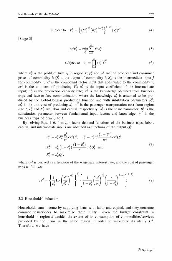
where pik is the profit of firm ik in region k; pi

k and qik are the producer and consumer

prices of commodity i; Qik is the output of commodity i; Xji

k is the intermediate input jfor commodity i; Vi

k is the compound factor input that adds value to the commodity i;cvi

k is the unit cost of producing Vik; aji

k is the input coefficient of the intermediate

input; avik is the production capacity rate; ji

k is the knowledge obtained from business

trips and face-to-face communication, where the knowledge jik is assumed to be pro-

duced by the Cobb-Douglas production function and with substitution parameters dnkl;

ctik is the unit cost of producing ji

k; skl is the passenger transportation cost from region

k to l; Lik and Ki

k are labor and capital, respectively; dik is the share parameter; bi

k is the

substitution parameter between fundamental input factors and knowledge; nikl is the

business trips of firm ik to l.By solving Eqs. 1–6, firm ik’s factor demand functions of the business trips, labor,

capital, and intermediate inputs are obtained as functions of the output Qik:

nkli ¼ ak

vidkln

bki

sklcvk

i Qki ; Lk

i ¼ akvid

ki

1� bki

� �

wkcvk

i Qki ;

Kki ¼ ak

vi 1� dki

� � 1� bki

� �

rcvk

i Qki ; and

Xkji ¼ ak

jiQki :

ð7Þ

where cvik is derived as a function of the wage rate, interest rate, and the cost of passenger

trips as follows:

cVli ¼

1

blj

Pl0sll0

dll0

n

!dll0n

8<

:

9=

;

blj

1

1� blj

wl

dlj

!dlj

r

1� dlj

!1�dlj

8<

:

9=

;

1�blj

ð8Þ

3.2 Households’ behavior

Households earn income by supplying firms with labor and capital, and they consume

commodities/services to maximize their utility. Given the budget constraint, a

household in region k decides the extent of its consumption of commodities/services

provided by the firms in the same region in order to maximize its utility Uk.

Therefore, we have

Nat Hazards (2008) 44:253–265 257

123

Uk dk� �

¼ maxdk

i

XM

i¼1

ðcki Þ

1rðdk

i Þr�1r

( ) rr�1

ð9Þ

subject toXM

i¼1

qki dk

i � yk ¼XM

i¼1

wkLki þ rKk

i

� �ð10Þ

where yk is income of the household which comprises the labor income and the rent on

capital, cik and r are the parameters of the model, and di

k is the demand for commodity i.By solving Eqs. 9 and 10, we obtain the following demand function:

dki ðqk; ykÞ ¼ ck

i ðqki Þ

1�r

PMi¼1 ck

i ðqki Þ

1�r

yk

qki

: ð11Þ

By substituting Eq. 11 in Eq. 9, the indirect utility function of a consumer is obtained as

Ukðqk; ykÞ ¼XM

i¼1

cki ðqk

i Þ1�r

( ) 1r�1

yk: ð12Þ

3.3 Interregional trade

The model consists of various regions, and the interregional trade needs to be described.

Our model assumes the iceberg formulation of transportation costs (Samuelson 1952), and

the transportation costs can be treated by evaporation of trading products themselves

during transport, instead of configuring unique transport sectors.

Let sikl denote the trade coefficient, i.e., the probability that industry i in region l buys

commodity i from region k. Consequently, we define the trade coefficient as

skli ¼

Qki exp �kip

ki 1þ /kl

i

� �� �PN

m¼1 Qmi exp �kip

mi 1þ /ml

i

� �� � ð13Þ

where /ikl is the rate of transportation cost which evaporates during transport, and ki

is a parameter. The trade coefficient represents the volume share of the commodity

demand. The term pik (1 + /i

kl) means the price of commodity i produced in region

k at region l. A higher pik (1 + /i

kl) means a smaller share in the consuming region

l. Applying Eq. 13, the following expression links the producer and consumer

prices:

qli ¼

XN

k¼1

pki 1þ /kl

i

� �skl

i : ð14Þ

Spatial price equilibrium theory is employed with regard to the interregional trade.

258 Nat Hazards (2008) 44:253–265

123

3.4 Equilibrium conditions before a disaster

Before a disaster occurs, a long-run equilibrium is assumed to be achieved without any

restrictions. The commodity market achieves equilibrium between regions with spatial

price equilibrium. The labor market is closed in each region and the capital market is

closed across the country. This assumption means that labor can move between sectors in a

region but cannot move between regions. This model considers these conditions as a set of

equilibrium conditions in an economic system prior to a disaster. Balances across all the

markets are described in the following manner.

First, the equilibrium conditions of the labor and capital markets areX

i

Lki ¼ Lk; ð15Þ

rX

k

X

i

Kki � K

!¼X

k

X

i

EXki �

X

k

X

i

IMki ; ð16Þ

where EXik and IMi

k denote the export and import to/from overseas countries, respectively.

In this paper, import and export are regarded as exogenous factors. They are added or

subtracted in advance.

Secondly, the equilibrium condition in the commodity market is formulated as

Qki ¼

XN

l¼1

skli dl

i þXM

j¼1

Xlij

( )1þ /kl

i

� �: ð17Þ

The left-hand side of Eq. 17 is the commodity supply from region k and the right-hand

side indicates a summation of the share of region k in the commodity demand in region l,while considering the transportation cost as a loss. In other words, the difference between

the right hand side and the left hand side equals the excess demand for commodity i in

region k.

Solving Eqs. 7, 11, 13, 15, 16, and 17 simultaneously, the equilibrium prices and

quantities of goods and factors are determined.

3.5 Equilibrium conditions after a disaster

In contrast to many other studies (see Okuyama and Chang 2004) conducted to date, this

study assumes no adjustments in labor, capital, and their prices, while allowing the

commodities and their prices to fluctuate across regions, when earthquakes cause a dis-

ruption in transport.

For convenience, the suffixes (0) and (1) are added in the following to distinguish the

variables before a disaster from those after a disaster. A new equilibrium will be derived

within this short-run equilibrium by solving the set of equations simultaneously, in which

the exogenous variables skl(0) and /ikl(0) are replaced by skl(1) and /i

kl(1), respectively.

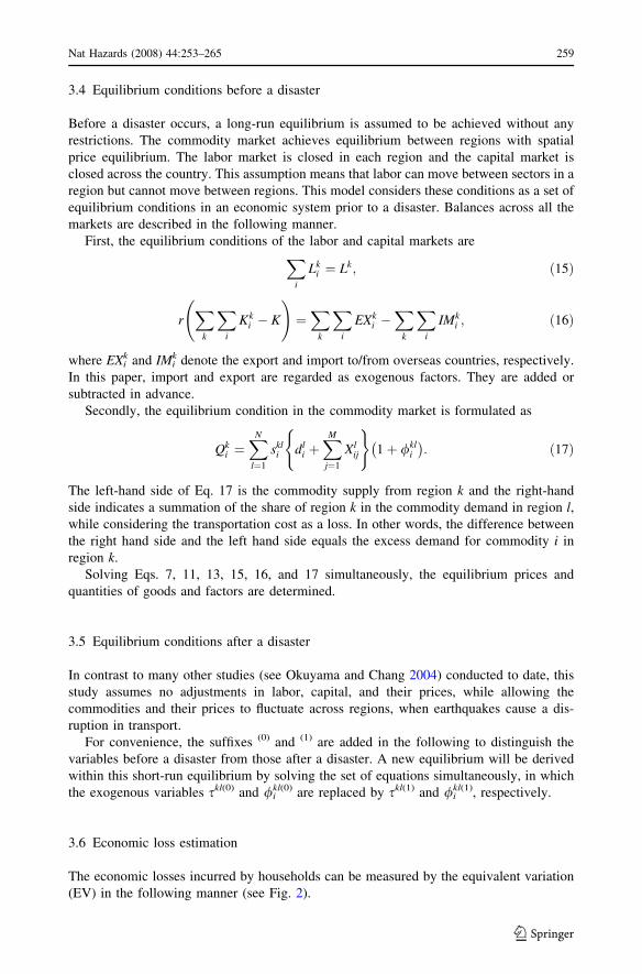
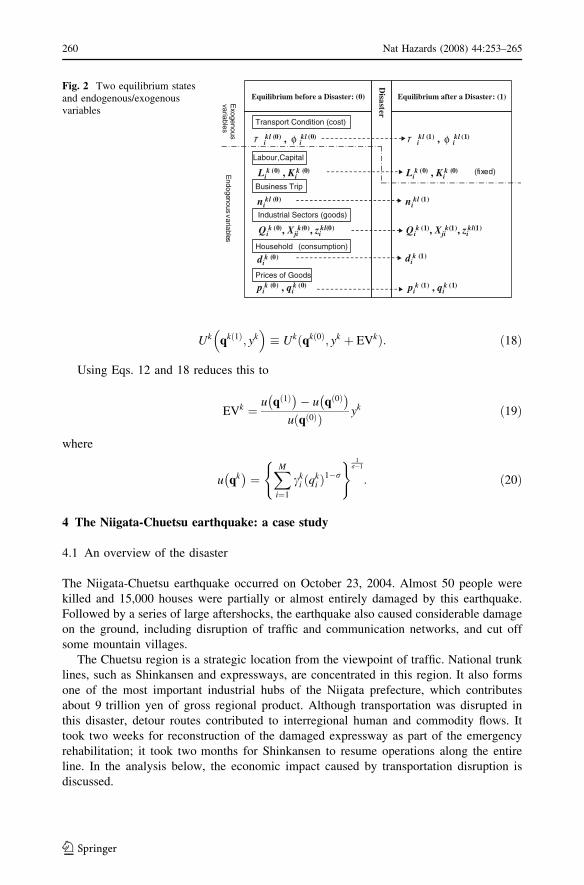
3.6 Economic loss estimation

The economic losses incurred by households can be measured by the equivalent variation

(EV) in the following manner (see Fig. 2).

Nat Hazards (2008) 44:253–265 259

123

Uk qkð1Þ; yk� �

� Ukðqkð0Þ; yk þ EVkÞ: ð18Þ

Using Eqs. 12 and 18 reduces this to

EVk ¼u qð1Þ� �

� u qð0Þ� �

u qð0Þð Þ yk ð19Þ

where

u qk� �

¼XM

i¼1

cki ðqk

i Þ1�r

( ) 1r�1

: ð20Þ

4 The Niigata-Chuetsu earthquake: a case study

4.1 An overview of the disaster

The Niigata-Chuetsu earthquake occurred on October 23, 2004. Almost 50 people were

killed and 15,000 houses were partially or almost entirely damaged by this earthquake.

Followed by a series of large aftershocks, the earthquake also caused considerable damage

on the ground, including disruption of traffic and communication networks, and cut off

some mountain villages.

The Chuetsu region is a strategic location from the viewpoint of traffic. National trunk

lines, such as Shinkansen and expressways, are concentrated in this region. It also forms

one of the most important industrial hubs of the Niigata prefecture, which contributes

about 9 trillion yen of gross regional product. Although transportation was disrupted in

this disaster, detour routes contributed to interregional human and commodity flows. It

took two weeks for reconstruction of the damaged expressway as part of the emergency

rehabilitation; it took two months for Shinkansen to resume operations along the entire

line. In the analysis below, the economic impact caused by transportation disruption is

discussed.

pik (0) , qi

k (0)Prices of Goods

Disaster

Transport Condition (cost)

Lik (0) , Ki

k (0)

Equilibrium before a Disaster: (0) Equilibrium after a Disaster : (1)

Lik (0) , Ki

k (0)

pik (1) , qi

k (1)

Household (consumption)

dik (0) di

k (1)

Qik (0), Xji

k(0), zikl(0) Qi

k (1), Xjik(1), zi

kl(1)

nikl (0) ni

kl (1)

ikl (0) , i

kl (0)ikl (1) , i

kl (1)

Endogenous variables

(fixed)

Labour,Capital

Business Trip

Industrial Sectors (goods)

Exogenous

variables

Fig. 2 Two equilibrium statesand endogenous/exogenousvariables

260 Nat Hazards (2008) 44:253–265

123

4.2 The database and parameters for quantitative analysis

An interregional input–output table that assumes economic equilibrium in a benchmark

year is necessary for the SCGE analysis. Many parameters are determined with this table

and with the conditions derived from firms’ behaviors. This analysis set the benchmark

year as 1995 due to the availability of statistical data.

The input–output database for this paper was prepared from the interregional input–

output table released by the Ministry of Economy, Trade, and Industry (METI), which

contains nine regions and three sectors trades, the input–output table of the Niigata pre-

fecture, and the national distribution census. The input–output of the Niigata prefecture

was used to decompose the directly affected area (Niigata prefecture) from the peripheries

(the rest of the Kanto region). The 1995 national distribution census, published by the

Ministry of Land, Infrastructure ,and Transport (MLIT), was used to estimate interregional

trade flow between Niigata and the other areas.

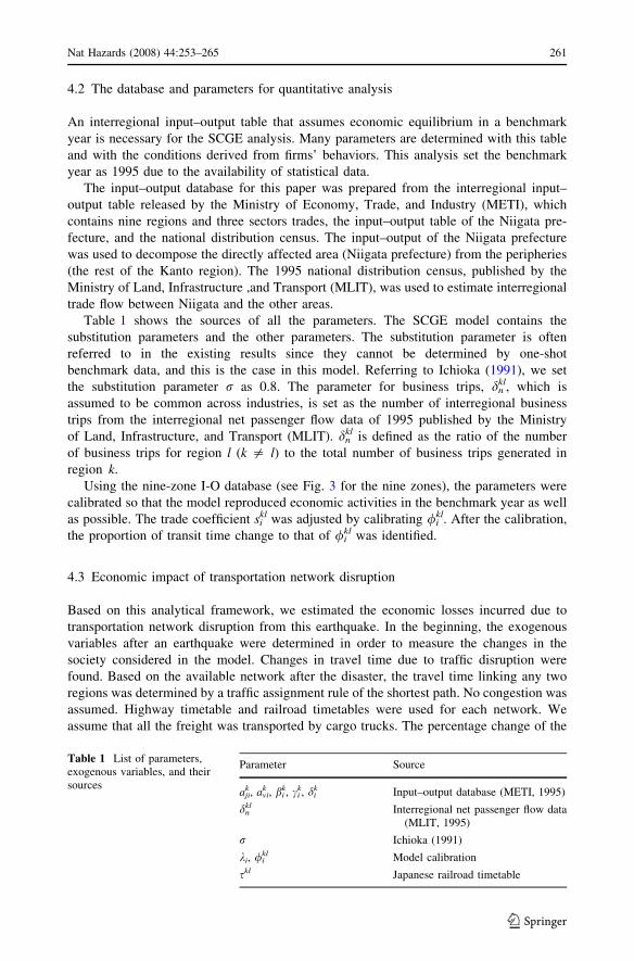
Table 1 shows the sources of all the parameters. The SCGE model contains the

substitution parameters and the other parameters. The substitution parameter is often

referred to in the existing results since they cannot be determined by one-shot

benchmark data, and this is the case in this model. Referring to Ichioka (1991), we set

the substitution parameter r as 0.8. The parameter for business trips, dnkl, which is

assumed to be common across industries, is set as the number of interregional business

trips from the interregional net passenger flow data of 1995 published by the Ministry

of Land, Infrastructure, and Transport (MLIT). dnkl is defined as the ratio of the number

of business trips for region l (k = l) to the total number of business trips generated in

region k.

Using the nine-zone I-O database (see Fig. 3 for the nine zones), the parameters were

calibrated so that the model reproduced economic activities in the benchmark year as well

as possible. The trade coefficient sikl was adjusted by calibrating /i

kl. After the calibration,

the proportion of transit time change to that of /ikl was identified.

4.3 Economic impact of transportation network disruption

Based on this analytical framework, we estimated the economic losses incurred due to

transportation network disruption from this earthquake. In the beginning, the exogenous

variables after an earthquake were determined in order to measure the changes in the

society considered in the model. Changes in travel time due to traffic disruption were

found. Based on the available network after the disaster, the travel time linking any two

regions was determined by a traffic assignment rule of the shortest path. No congestion was

assumed. Highway timetable and railroad timetables were used for each network. We

assume that all the freight was transported by cargo trucks. The percentage change of the

Table 1 List of parameters,exogenous variables, and theirsources

Parameter Source

ajik , avi

k , bik, ci

k, dik Input–output database (METI, 1995)

dnkl Interregional net passenger flow data

(MLIT, 1995)

r Ichioka (1991)

ki, /ikl Model calibration

skl Japanese railroad timetable

Nat Hazards (2008) 44:253–265 261

123

transit time in the vicinity of the disaster is reflected in the change of /ikl; all commuters

making business trips were assumed to use the railroad. The generalized travel cost (skl)

was the sum of the passenger fare and travel time and was measured in terms of monetary

value. After the disaster, some passengers had to make a detour due to disruption. Con-

sequently, the generalized travel cost before a disaster skl(0) was replaced by the cost after

the disaster skl(1).

The transportation disruption scenario caused by the disaster is summarized as follows.

• First period: until the 13th day after the earthquake occurred.

In this period, both the highway/expressway and railroad linking Tokyo (Kanto region)

and Niigata prefecture were disrupted. Freight transit time between Kanto and Niigata

increases by 25%, and the generalized travel costs for business trips from/to Niigata

rise by 9*30%.

• Second period: from the 14th to 66th day.

The disrupted roads were rehabilitated and only business trips were affected in this

period because of railroad transport disruption. For model inputs, we use the same

generalized travel costs as the first period, and freight transit time before the disaster.

Figure 4 shows the losses to the entire nation for the first period due to disruptions in the

transportation network. The transport-related losses are estimated according to transpor-

tation mode: trucks for commodity transport and trains for passenger trips. The share of

each mode to the total losses for the first period is almost 50%. It is found that the loss

under the simultaneous disruption scenario of the two transportation modes is not exactly

Fig. 3 Regions and transportation networks: (a) the nine zones for loss estimation, (b) major expressway/highway network, (c) major rail network and detour routes

262 Nat Hazards (2008) 44:253–265

123

equal to the sum of the losses when each mode is separately disrupted, although the

difference is extremely small in this case study. Because of this interactive effect, the loss

should be simultaneously measured for multiple disruption scenarios.

Figure 5 presents the regional economic losses arising from transportation disruptions

from the Niigata-Chuetsu earthquake. The impact of the disruption in the Tokyo-Niigata

transportation links spreads across the region. The whole cumulative transport-related

losses accounts amount to 9.2 and 19.0 billion yen for the first and second period,

respectively. Nearly 40% of the total losses are attributable to the Kanto region because of

its geographical location and economic importance. The Niigata prefecture suffers the

second largest losses of 5.5 billion yen, or 20% of the total losses. Tohoku, Chubu, and

Kinki regions share about 10% each, and the other 10% falls on the four regions Hokkaido,

Chugoku, Shikoku, and Kyushu-Okinawa.

Compared to the interregional transport, the transit time for intraregional commodity

transport is not easy to set, since the model treats each zone as a centroid. Sensitivity

0.0

2.0

4.0

6.0

8.0

10.0

12.0

14.0

(billion yen)

Bar ChartCumulative losses during the 1st periodCumulative losses during the 2nd period

Line Plot --Cumulative losses during the 1st period when

intra-regional transit time of Niigata prefectureincreases by:

10% (0.1 hour), 25%, 75%, 100%.

(base case: 50% = 0.5 hour)

Kyushu &Okinawa

ShikokuChugokuKinkiChubuNiigataKantoTohokuHokkaido

Fig. 5 The total transport-related losses by region

0.0

2.0

4.0

6.0

8.0

10.0

45.6

Highway Disruption Scenario(WO: No disruption, W: Disruption)

46.5

92.1

0.0

(billion yen)

WW

Railroad Disruption Scenario(WO: No disruption,

W: Disruption)

WO

W

Fig. 4 The cumulative transport-related losses during the first period

Nat Hazards (2008) 44:253–265 263

123

analysis on the intraregional transit time in the Niigata prefecture shows that the estimated

losses to Niigata can change greatly if the intraregional time changes significantly. The line

plots in Fig. 5 are cumulative losses during the first period with different transit time

inputs. Compared to the base case, in which it takes 30 min more than usual for commodity

transit inside Niigata prefecture, the cumulative losses for the first period can rise by 60%

if the intraregional transit time doubled.

For passenger transport, the model mainly considers the railroad network, and assumes

that alternative buses are available for detours while the transportation network is dis-

rupted. One more real alternative mode was airline travel between Tokyo and Niigata, for

which there is no service ordinarily. In this case, losses due to passenger transport dis-

ruption would be lower than predicted by the model simulation. However, airline service

was not comparable to Shinkansen in terms of transport capacity and frequency, as the

Shinkansen network has such a high capacity and frequency. Thus it is hard to compare the

service provided by Shinkansen in terms of generalized costs only. This is why the model

only considers ground transportation.

5 Conclusion

This paper presented an analytical framework to estimate the economic losses incurred due

to transportation network disruption after a catastrophic earthquake. The spatial comput-

able general equilibrium model developed in this paper can capture properties involving

time and integration with the transportation network. First, a short-run equilibrium is

emphasized and the labor and capital markets are restricted with respect to their adjust-

ments in response to a change in the external conditions arising from an earthquake.

Secondly, two types of transportation networks are considered in the model: the road

network for the transport of freight and the railway network for passenger trips.

The model was applied to estimate the transport-related loss arising from the Niigata-

Chuetsu earthquake. The loss was considerable and spread across multiple regions. This

observation implies that countermeasures are needed to reduce negative spillovers to the

unaffected regions as well as the adoption of mitigation policies for the reduction of

damage to houses and facilities. For future research, further aspects of transportation such

as road traffic congestion and service frequency of passenger trips could be incorporated

into this model.

There are other aspects to be incorporated within the loss estimation framework. The

SCGE model is such a promising approach in the context of disaster management that it

can be developed into a more-sophisticated framework by integrating, for example, pro-

duction capital loss and lifeline disruptions.

References

Cadiou L, Dees S, Laffargue JP (2003) A computable general equilibrium model with vintage capital.J Econ Dyn Control 27:1961–1991

Gordon P, Richardson H, Davis B (1998) Transport-related impacts of the Northridge earthquake. J TranspStat 1(2):21–36

Ichioka O (1991) Applied general equilibrium analysis. Yuhikaku (in Japanese)Okuyama Y, Chang SE (2004) Modeling spatial and economic impacts of disasters (Advances in spatial

science). Springer-Verlag, BerlinRose A (2004) Economic principles, issues, and research priorities in hazard loss estimation. In: Okuyama

Y, Chang SE (eds) Modeling spatial and economic impacts of disasters (Advances in spatial science).Springer-Verlag, Berlin, pp 13–36

264 Nat Hazards (2008) 44:253–265

123

Rose A, Benavides J (1998) Regional economic impacts. In: Shinozuka M, Rose A, Eguchi RT (eds)Engineering and socioeconomic impacts of earthquakes—an analysis of electricity lifeline disruptions inthe New Madrid area. Multidisciplinary Center for Earthquake Engineering Research, USA, pp 95–124

Rose A, Guha G (2004) Computable general equilibrium modeling of electric utility lifeline losses fromearthquakes. In: Okuyama Y, Chang SE (eds) Modeling spatial and economic impacts of disasters(Advances in spatial science). Springer-Verlag, Berlin, pp 119–142

Rose A, Liao S (2005) Modeling regional economic resilience to disasters: a computable general equilib-rium analysis of water service disruptions. J Reg Sci 45(1):75–112

Samuelson P (1952) The transfer problem and transport costs: the terms of trade when impediments areabsent. Econ J 62:278–304

Sohn J, Hewings GJD, Kim TJ, Lee JS, Jang SG (2004) Analysis of economic impacts of an earthquake ontransportation network. In: Okuyama Y, Chang SE (eds) Modeling spatial and economic impacts ofdisasters (Advances in spatial science). Springer-Verlag, Berlin, pp 233–256

Toyoda T, Kochi A (1997) Estimation of economic damages in the industrial sector by the great Hanshin-Awaji earthquake. J Polit Econ Commer Sci 176(2):1–16 (in Japanese)

Ueda T, Koike A, Iwakami K (2001) Economic damage assessment of catastrophe in high speedrail network. Proceedings of 1st workshop for ‘‘Comparative Study on Urban Earthquake DisasterManagement,’’ pp 13–19, Kobe, Japan, Jan. 18–19, 2001 http://www.drs.dpri.kyoto-u.ac.jp/us-japan/first.html

Varian HR (1992) Micro economic analysis, 3rd edn. WW Norton & Co Inc., p 563

Nat Hazards (2008) 44:253–265 265

123