A comprehensive study across methods and time scales to estimate surface fluxes from Lake Kinneret,...

This article appeared in a journal published by Elsevier. The attachedcopy is furnished to the author for internal non-commercial researchand education use, including for instruction at the authors institution

and sharing with colleagues.

Other uses, including reproduction and distribution, or selling orlicensing copies, or posting to personal, institutional or third party

websites are prohibited.

In most cases authors are permitted to post their version of thearticle (e.g. in Word or Tex form) to their personal website orinstitutional repository. Authors requiring further information

regarding Elsevier’s archiving and manuscript policies areencouraged to visit:

http://www.elsevier.com/copyright

http://www.elsevier.com/copyright

Author's personal copy

A comprehensive study across methods and time scales to estimate surfacefluxes from Lake Kinneret, Israel

Alon Rimmer a,*, Rana Samuels b, Yuri Lechinsky a

a Israel Oceanographic and Limnological Research Ltd., The Yigal Alon Kinneret Limnological Laboratory, P.O.B. 447, Migdal 14950, Israelb Department of Geophysics and Planetary Sciences, Faculty of Exact Sciences, Tel Aviv University, Tel Aviv 69978, Israel

a r t i c l e i n f o

Article history:Received 18 June 2009Received in revised form 8 September 2009Accepted 5 October 2009

This manuscript was handled by K.Georgakakos, Editor-in-Chief, with theassistance of A.A. Tsonis, Associate Editor

Keywords:Surface fluxesLatent heat fluxSensible heat fluxEvaporation methodsEnergy balanceHeat storage

s u m m a r y

Estimation of surface fluxes in general, and evaporation rates over lake surfaces in particular, is a difficulttask. While previous studies of Lake Kinneret, Israel, have looked at evaporation rate using a single time-scale or single measurement method, this is the first comprehensive study to reconcile and explain thedifferences between a variety of measurement and calculation methods (pan evaporation, water and heatbalance, aerodynamic methods and Penman simplified methods) across a multitude of temporal scales(10 min, 1 h, daily, monthly). The cross validation of the methods suggests that the hourly calculationwith the aerodynamic methods may result in a better estimation of the monthly Bowen Ratio for theenergy balance methods, and therefore may increase its reliability. We also show that comprehensivemeasurements and calculations of monthly heat storage change in the lake can be used to verify thehourly results of the hydrodynamic method, and the daily calculations of the Penman’s equation method.Moreover, using the Penman’s equation it is suggested that daily Pan A evaporation measurements arenearly similar to the evaporation from the deep water lake when the heat storage change is not taken intoaccount. It is suggested that subject to data availability, the cross validation of multiple methodsincreases the reliability and confidence of the measured and calculated surface fluxes.

� 2009 Elsevier B.V. All rights reserved.

Introduction

Estimation of surface fluxes in general, and evaporation ratesover lake surfaces in particular, is a difficult task given the multi-tude of factors involved in these processes, the various time scales,and the type of measurements needed to verify the estimations.(i.e. net radiation, heat energy of inflows and outflows, meteoro-logical variables governing the sensible and latent heat fluxes, spa-tial distribution of these variables and heat storage change in thelake). Consequently, a multitude of methods exists for the mea-surement and estimation of these fluxes (Morton, 1986; Gianniouand Antonopoulos, 2007), each method with its specific advantagesand disadvantages: (1) The water and energy budget approach(Winter, 1981; Assouline, 1993 – Lake Kinneret), is considered asthe most accurate method for long term periods, however, beingapplied usually on a monthly basis, it uses the monthly averagedBowen Ratio, a value not physically valid for long time periods(Assouline and Mahrer, 1993). (2) Pan A measurements (Ponce,1989) obviously reflect the conditions for evaporation, but the re-sults are usually applied for potential evaporation from shallowwet surfaces rather than deep lakes where heat storage plays animportant role. (3) The eddy correlation technique (Assouline

and Mahrer, 1993 – Lake Kinneret; Tanny et al., 2008) is consideredthe most reliable and accurate for direct evaporation estimation,however this method is difficult to perform since it requires spe-cialized and highly accurate instrumentation, and is therefore bestsuited for short-term observations (Ikebuchi et al., 1988). (4) Thehydrodynamic methods are the most popular technique for esti-mation of water surface fluxes (Rayner, 1980; Imberger and Patter-son, 1990; Imboden and Wüest, 1995; Fairall et al., 1996; Gal et al.,2003 – Lake Kinneret), but although they are physically based, andeasily applied for short time intervals, their results are difficult toverify on the basis of energy balance because of the difficulties inestimation of the short-term net vertical heat flux into the watercolumn. (5) The simplified energy budget related methods (Brutsa-ert, 1982; Katul and Parlange, 1992; Allen et al., 1998; Valiantzas,2006; Tanny et al., 2008) originate from hydrological and agricul-tural considerations, and therefore are based on meteorologicalmeasurements at a single elevation above the surface. This methodis especially useful for evaporation estimations when data from thelake itself do not exist. Unlike other methods it was never testedfor Lake Kinneret.

The purpose of this study is to present an improved understand-ing of the role of surface fluxes in the energy balance of Lake Kin-neret (northern Israel) using various methods and a large database. In addition, it serves to verify this suite of methods for calcu-lating evaporation and sensible heat flux across a multitude of time

0022-1694/$ - see front matter � 2009 Elsevier B.V. All rights reserved.doi:10.1016/j.jhydrol.2009.10.007

* Corresponding author. Tel.: +972 4 4909320.E-mail address: [email protected] (A. Rimmer).

Journal of Hydrology 379 (2009) 181–192

Contents lists available at ScienceDirect

Journal of Hydrology

journal homepage: www.elsevier .com/ locate / jhydrol


scales. Lake Kinneret is the only freshwater surface lake in thecountry and provides about 35% of the annual water supply. Evap-oration accounts for between 35–50% of water losses during anygiven year and plays an important role in determining the salinityof the lake (Rimmer, 2003, 2007). Evaporation rates have been alsoshown to have important impacts on water quality in the lake(Hambright et al., 2000; Gal et al., 2003), hence a better under-standing of evaporation rates at a multitude of time scales isneeded for water planning and management, as well as an im-proved understanding of limnological processes. Currently, sys-tematic evaporation calculations are based on a single mass andenergy balance method (Assouline 1993; Mekorot, 1987–2008,21 annual reports of Lake Kinneret water, solutes and heat bal-ances) using meteorological data from a single location. However,the multiple measurements currently available from the lake area(the type of data used in this study are elaborated in Table 1) andthe multiple available calculation techniques call for an improvedand comprehensive understanding that will enable identificationof methods which can provide consistent surface flux estimatesat different time scales, and for various purposes.

To this end, we apply seven different algorithms for calculatingevaporation rates and compare the results and variables of the dif-ferent approaches at different time scales. The seven algorithms in-clude: (1) Pan A evaporation measurements and its annual trendanalysis; (2) Heat balance calculations; (3–4) two different algo-rithms of aerodynamic methods with atmospheric stability consid-erations, (5) Empirical algorithm of the aerodynamic method; (6)the Penman approach for daily calculations of surface fluxes; and(7) the Penman–Brutsaert method, which is an intermediate algo-rithm between the Penman approach and the aerodynamic meth-ods. The usage of several methods, compared to various measuredvariables and using data from a multitude of meteorological sta-tions increases the confidence of current surface fluxes estimationsboth from the lake itself as well as from the surroundingwatershed.

The next section (Section ‘‘Study area, physical measurementsand typical trends”) describes the area of Lake Kinneret, and thenature of the physical and meteorological measurements takenboth in and around the lake. It also presents evaporation analysisbased on Pan A measurements at the vicinity of the lake shore,and the considerations of lake heat storage measurements. The fol-

lowing section, ‘‘Energy budget”, describes the fundamentals of theenergy balance calculations and the associated surface flux mea-surements. Section ‘‘Methods of surface fluxes analysis” describesthe monthly energy balance method, the short time scale aerody-namic method, the daily Penman’s approach, and discusses the re-sults of each method. In the final section, ‘‘Discussion”, we comparethe measurements, calculations and assumptions specific to eachof the methods and suggest how they can be integrated andcross-validated to inform one another. In the ‘‘Appendix” we pro-vide a table listing the symbols used throughout the paper as con-stants, parameters and variables for the surface fluxes analysis.

Study area, physical measurements and typical trends

Lake description

Lake Kinneret is a natural monomictic lake located in the north-ern part of Israel (Fig. 1). It is the most important surface water re-source in the country providing 35% of annual drinking waterthrough the National Water Carrier (NWC) canal and local pump-ing. The average area of the lake surface is 166 km2, the averagevolume is 4100 Mm3, the average annual available water is�450 Mm3, and the average residence time is �8–10 years. TheJordan River is the major inflow to the lake, while the waterpumped into the NWC constitutes the major outflow. The Lake isreplenished during the colder rainy season which lasts fromaround October to April.

Meteorological measurements

Physical meteorological measurements are taken from four sta-tions located around and offshore Lake Kinneret (Table 1, Fig. 1).The major source for the current study is the Tabgha Station (MTin Fig. 1) with data available since 1996. The station is locatedabove the lake surface, �700 m offshore (35�33.01 E and32�51.95 N), at an elevation of �210 ASL. The station providesthe following data at 10 min time intervals: air temperature (�C)and relative humidity are measured using YOUNG relative humid-ity and temperature probe model 43372C, at �5 m above water le-vel. Global short wave radiation (305–2800 nm, W m�2) measuredwith Kipp & Zonen DELFT BV shortwave radiometer CM11, at �5 m

Table 1Summary of data type and data sources used in this study.

Type of data Years Source Time scale Remarks

1 Measured and calculated stream flow, spring discharge and directrainfall on Lake Kinneret

1987–2008 IHS, Mekorot Daily (con.) Used in water balance

2 Meteorological measurements (air temperature, water surfacetemperaturea, relative humidity, global radiation, long waveradiationa, wind speed, wind direction) from 5 stations onshoreand on the surface of Lake Kinneret

1987–2008 KLL, IMS, Mekorot 10–60 min (frc.) Various starting dates in stations

3 Pan evaporation from 15 stations in the Lake Kinneret watershed 1970–2008 IMS, ASUGRC, Mekorot Daily (frc.) Various starting dates in stations4 Water consumption from Lake Kinneret 1987–2008 IWA, Mekorot Monthly (con.) Used in water balance5 Heat storage of Lake Kinneret, based on manual heat profile

measurements in 45 locations, distributed around the lake areaduring a 4 h survey

1986–2008 Mekorot Monthly (con.) Used in water balance

6 Manual heat profile measurements in the center of the lake 1969–2008 KLL Weekly (con.) Various starting dates7 Automated heat profile measurements in the center of the lake 1999–2008 KLL, CWR 10 min (frc.)

IHS: Israel Hydrological Service.IMS: Israel Meteorological Service.IWA: Israel Water Authority.ASUGRC: Agrometeorology Services of the Upper Galilee Regional Council.KLL: Kinneret Limnological Laboratory.Mekorot: Israel National Water Supply Company.CWR: Center of Water Research, university of Western Australia.frc.: Data are fractured to various time periods.con.: Data are continuous for the entire period.

a Measurements in Tabgha station only.

182 A. Rimmer et al. / Journal of Hydrology 379 (2009) 181–192


above water level. Wind speed and direction measured with Youngwind monitor MA-05106, at �8 m above sea level. Downwellinglongwave radiation (5–25 nm W m�2) measured by KIPP & ZONENDELFT BV longwave radiometer CG1, at �5 m above water level.Water surface temperature (�C) measured by YOUNG platinumfloating temperature probe model 41342, at a depth of �0.05 m.Other stations (Beit Zeida – BZ, Station A – TA and Tzemach – TZin Fig. 1) provide temperature, global radiation, and wind speedand direction with similar equipment.

The seasonal and diurnal trends of air temperature, water sur-face temperature, long wave radiation, short wave radiation,humidity and wind speed for the year 2005 at the Tabgha stationare shown in Fig. 2. While the diurnal oscillations are oftendamped out at the daily scale, they provide important informationfor hourly calculations, necessary for understanding the dynamicsof the meteorology in the lake area.

Throughout the entire year low wind speed (<2 m s�1) is typicalbetween the hours 00:00 to 10:00, but during the summer monthsa daily north-westerly wind, caused by the Mediterranean Seabreeze (�10–15 m s�1), reaches the surface of the lake, and usuallypeaks at 15:00 (U in Fig. 2). The relative humidity (RH in Fig. 2) isinversely correlated with the wind speed because the wind re-moves the wet air above the lake surface bringing dry air fromthe land, and reducing RH by �20% above the lake surface. Air tem-perature (Ta in Fig. 2) fluctuates annually between daily means of12–32 �C. Together with intense short and long wave radiation(RSWin and RLWin in Fig. 2, respectively) this results in the lake beingstrongly temperature stratified from about mid-April to lateDecember. Typical water surface temperature (Ts in Fig. 2) variesfrom between �15 �C in January to �30 �C in August while thehypolimnion temperatures remains at �15 �C throughout the year.The daily temperature variations of the air are by far larger thanthe variations of daily water surface temperature. The thermocline

depth (defined as the peak temperature gradient throughout thewater profile) is located at around the depth of �10 m in April,and then it drops to a depth of �14, and�17 m by June and August,respectively, and finally to �30 m just before the lake overturn inDecember–January.

Typical annual trends

A simple cross validation between various calculated/measuredmethods of surface fluxes using different timescales is carried outby comparing the results of the meteorological parameters to thelong term means of daily averages. Mean annual trends can oftenbe calculated for each of the meteorological parameters, usingthe results of mass and energy balance, approximated with anempirical equation of the form:

Y ¼ b½1þ a� sinðk � ðJDþxÞÞ� ð1Þ

where Y is the parameter being calculated, JD is the day of the year,a and b are constants, x is the phase shift, and k is the angular fre-quency in radians which for characteristics with yearly rotationshas a set value of k ¼ 2� p=365:25. The typical annual trends of se-lected meteorological variables are characterized by the parametersin Table 2, and will be used later as a reference for variouscalculations.

Lake temperature measurements

Two types of lake temperature measurements are relevant tothis study (Table 1).

(1) For the monthly energy balances (Section ‘‘The monthlyenergy balance”) conducted by Mekorot (Israel NationalWater Co.) since 1987, temperature profiles were measuredon a monthly basis using STD-12 Plus (Applied Microsys-tems Ltd.) with an error of ±0.005 �C. The device monitoredprofile temperatures at 45 locations distributed around thelake area during a 4 h survey. The large number of profilesreduces the uncertainties associated with the calculationsof the heat storage due to internal heat waves (Antenucciet al., 2000).

(2) For short time analysis of lake temperature, profileswere measured at Station TA (center of the lake, seeFig. 1) using Precision Measurement Engineering (PME)Thermistor Chain, a single cable thermistor chain with40 thermistors along the cable at 1 m intervals (every20 s). Temperatures were measured with an error of±0.005 �C.

Pan A evaporation

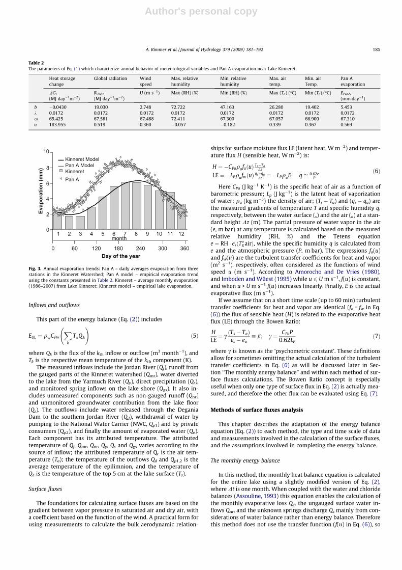
Long term measurements of Pan A evaporation in the Upper Jor-dan River catchments and Lake Kinneret area (Table 1) are usedhere to provide an additional reference trend. Measurements weretaken as described by Ponce (1989). The typical annual trend ofthese evaporation measurements was calculated using the empir-ical Eq. (1), with the specific attributed parameter values as shownin Table 2. Daily means of Pan A evaporation from three stations for30 years, and monthly means of evaporation from Lake Kinneretfor 21 years are shown in Fig. 3, together with the results of theempirical trend for both cases (Eq. (1)). There are significant differ-ences between the annual trends of Pan A evaporation and LakeKinneret evaporation measurements (Fig. 3). The physical causesfor these differences will be discussed in Section ‘‘Penmanapproach”.

-215-220

-225 -230-235

-245

-240

-250

32o54’

32o48’

32o52’

32o50’

32o46’

32o44’

35o35’

35o37’

35o31’

35o33’

35o39’

Jordan River N.

0 3

km

6

TZ

Lake Kinneret

N

32o42’

MT

TA

BZ

NWC

Jordan River S.-215-220

-225 -230-235

-245

-240

-250

o ’

o ’

o ’

o ’

o ’

o ’

o’

o’

o’

o’

o’

Jordan River N.

0 3

km

6

TZ

Lake Kinneret

N

o ’

MT

TA

BZ

NWC

Jordan River S.

Fig. 1. Location of Lake Kinneret and the four meteorological stations: Station A(TA), Tabgha (MT), Tzemach (TZ), and Beit Zidah (BZ).

A. Rimmer et al. / Journal of Hydrology 379 (2009) 181–192 183


Energy budget

The general energy budget equation is based on the conservationof energy law, which accounts for incoming and outgoing energy,balanced by the amount of energy stored in the system. It shouldbe noted however, that the following equation of energy balancedoes not include changes of potential, kinetic, or biological energy,since these are orders of magnitude smaller than the heat energy(Imberger, 1985; Imboden and Wüest, 1995). Omitting these com-ponents, the energy balance equation, for an average square meterof the lake, and for a certain period of time Dt can be calculated as:

DGL

AL¼ Rn þ

EQL

AL� ðLEþ HÞ

� �Dt ð2Þ

where DGL (J) is the change in heat storage in the lake per unit oftime, AL (m2) is the lake water surface, Rn (W m�2) is the net radia-tion on the lake surface, EQL (J t�1) is the total net heat advectionfrom inflows and outflows including withdrawal of evaporatedwater, LE (W m�2) the latent heat fluxes and H (W m�2) the sensibleheat flux over the surface of the lake. Eq. (2) does not take into ac-count heat entering from the floor of the lake, since this is consid-ered negligible in Lake Kinneret, other than the contribution ofthe saline springs (Rimmer and Gal, 2003) which enter Eq. (2)through the EQL component. The following sections describe thecomponents of the energy balance equation.

Measurements of heat storage changes

The change in the heat storage of the water body (DGL) can bedetermined by measurements of the lake’s temperature using athermistor chain stretched throughout the entire water profile.The measurements can be taken at various time intervals depend-ing on the time scale of the heat budget desired (e.g., hour, day,week or month). The heat storage change can then be calculated by:

DGL ¼ GLjt2� GLjt1

GLðtÞ ¼ CPwR z¼zm

z¼0 qwðz; tÞTwðz; tÞAðzÞdzð3Þ

where CPw (J kg�1 K�1) is the specific heat capacity of water, A(z) isthe horizontal surface area (m2) as a function of elevation z, zm is thelake level, Tw(z, t) is the water temperature measurement at eleva-tion z and time t, and qw(z, t) is the attributed water density. Itshould be noted, however, that continuous GL measurements basedon a single thermistor chain location can produce large measurederrors in DGL due to internal waves that may alter significantlythe distribution of temperature in deep layers during time. Theusage of DGL within the calculations of short-term energy balanceis therefore not trivial. This issue will be discussed further in Sec-tion ‘‘Aerodynamic method”.

Net radiation

The net radiation Rn is computed from meteorological monitor-ing. It can either be measured directly, or calculated with therelation:

Rn ¼ RSWin � RSWout þ RLWin � RLWout

RSWout ¼ aSWRSWin

RLWout ¼ aLWRLWin þ BeT4s

ð4Þ

where RLWin and RSWin are the measured incoming long and shortwave radiation, respectively; RLWout and RSWout are the calibratedoutgoing long and short wave radiation, respectively; the parame-ters aLW and aSW are calibrated reflection constants for long andshort wave radiation, respectively, and BeT4

s is the emitted longwave radiation from the lake surface calculated from the surfacetemperature Ts, the Boltzman constant, B, and the emissivity ofthe lake surface e.

23456789

101112

40455055606570

123456789

16182022242628

141618202224262830

0 5 10 15 20320

340

360

380

400

420

123456789

101112

mon

th

0 5 10 15 20

100200300400500600700800

hour

23456789

101112

RH

Ta

RSWinRLWin

Ts

U

Fig. 2. Typical seasonal and diurnal trends of air temperature (Ta, �C), water surface temperature (Ts, �C), long wave radiation (RLWin, W m�2), short wave radiation (RSWin,W m�2), relative humidity (RH, %) and wind speed (U, m s�1) for the year 2005 at the Tabgha station.



Inflows and outflows

This part of the energy balance (Eq. (2)) includes

EQL ¼ qwCPw

Xk

TkQ k

!ð5Þ

where Qk is the flux of the kth inflow or outflow (m3 month�1), andTk is the respective mean temperature of the kth component (K).

The measured inflows include the Jordan River (Qj), runoff fromthe gauged parts of the Kinneret watershed (Qmr), water divertedto the lake from the Yarmuch River (Qy), direct precipitation (Qr),and monitored spring inflows on the lake shore (Qgs). It also in-cludes unmeasured components such as non-gauged runoff (Qnr)and unmonitored groundwater contribution from the lake floor(Qs). The outflows include water released through the DeganiaDam to the southern Jordan River (Qd), withdrawal of water bypumping to the National Water Carrier (NWC, Qp1) and by privateconsumers (Qp2), and finally the amount of evaporated water (Qe).Each component has its attributed temperature. The attributedtemperature of Qj, Qmr, Qnr, Qy, Qs and Qgs varies according to thesource of inflow; the attributed temperature of Qr is the air tem-perature (Ta); the temperature of the outflows Qd and Qp1,2 is theaverage temperature of the epilimnion, and the temperature ofQe is the temperature of the top 5 cm at the lake surface (Ts).

Surface fluxes

The foundations for calculating surface fluxes are based on thegradient between vapor pressure in saturated air and dry air, witha coefficient based on the function of the wind. A practical form forusing measurements to calculate the bulk aerodynamic relation-

ships for surface moisture flux LE (latent heat, W m�2) and temper-ature flux H (sensible heat, W m�2) is:

H ¼ �CPaqafaðuÞ Ts�TaDz

LE ¼ �LPqafwðuÞ qs�qaDz � �LPqaE; q ffi 0:62e

P

ð6Þ

Here CPa (J kg�1 K�1) is the specific heat of air as a function ofbarometric pressure; Lp (J kg�1) is the latent heat of vaporizationof water; qa (kg m�3) the density of air; (Ts � Ta) and (qs � qa) arethe measured gradients of temperature T and specific humidity q,respectively, between the water surface (s) and the air (a) at a stan-dard height Dz (m). The partial pressure of water vapor in the air(e, m bar) at any temperature is calculated based on the measuredrelative humidity (RH, %) and the Tetens equatione ¼ RH � esðTo

K airÞ, while the specific humidity q is calculated frome and the atmospheric pressure (P, m bar). The expressions fa(u)and fw(u) are the turbulent transfer coefficients for heat and vapor(m2 s�1), respectively, often considered as the functions of windspeed u (m s�1). According to Amorocho and De Vries (1980),and Imboden and Wüest (1995) while u 6 U m s�1, f(u) is constant,and when u > U m s�1 f(u) increases linearly. Finally, E is the actualevaporative flux (m s�1).

If we assume that on a short time scale (up to 60 min) turbulenttransfer coefficients for heat and vapor are identical (fa = fw in Eq.(6)) the flux of sensible heat (H) is related to the evaporative heatflux (LE) through the Bowen Ratio:

HLE¼ cðTs � TaÞes � ea

� b; c ¼ CPaP0:62LP

ð7Þ

where c is known as the ‘psychometric constant’. These definitionsallow for sometimes omitting the actual calculation of the turbulenttransfer coefficients in Eq. (6) as will be discussed later in Sec-tion ‘‘The monthly energy balance” and within each method of sur-face fluxes calculations. The Bowen Ratio concept is especiallyuseful when only one type of surface flux in Eq. (2) is actually mea-sured, and therefore the other flux can be evaluated using Eq. (7).

Methods of surface fluxes analysis

This chapter describes the adaptation of the energy balanceequation (Eq. (2)) to each method, the type and time scale of dataand measurements involved in the calculation of the surface fluxes,and the assumptions involved in completing the energy balance.

The monthly energy balance

In this method, the monthly heat balance equation is calculatedfor the entire lake using a slightly modified version of Eq. (2),where Dt is one month. When coupled with the water and chloridebalances (Assouline, 1993) this equation enables the calculation ofthe monthly evaporative loss Qe, the ungauged surface water in-flows Qnr, and the unknown springs discharge Qs mainly from con-siderations of water balance rather than energy balance. Thereforethis method does not use the transfer function (f(u) in Eq. (6)), so

Table 2The parameters of Eq. (1) which characterize annual behavior of meteorological variables and Pan A evaporation near Lake Kinneret.

Heat storagechange

Global radiation Windspeed

Max. relativehumidity

Min. relativehumidity

Max. airtemp.

Min. airTemp.

Pan Aevaporation

DGL

(MJ day�1m�2)RSWin

(MJ day�1m�2)U (m s�1) Max (RH) (%) Min (RH) (%) Max (Ta) (�C) Min (Ta) (�C) EPanA

(mm day�1)

b �0.0430 19.030 2.748 72.722 47.163 26.280 19.402 5.453k 0.0172 0.0172 0.0172 0.0172 0.0172 0.0172 0.0172 0.0172x 65.425 67.581 67.488 72.411 67.300 67.057 66.900 67.310a 183.955 0.519 0.360 �0.057 �0.182 0.339 0.367 0.569

0

2

4

6

8

10

0 60 120 180 240 300 360Day of the year

Evap

orat

ion

(mm

)

Pan A

Pan A ModelKinneret

1 2 3 4 5 6 7 8 9 10 11 12month

Kinneret Model

Fig. 3. Annual evaporation trends: Pan A – daily averages evaporation from threestations in the Kinneret Watershed; Pan A model – empirical evaporation trendusing the constants presented in Table 2. Kinneret – average monthly evaporation(1986–2007) from Lake Kinneret; Kinneret model – empirical lake evaporation.



that wind speed measurements are actually not included in thecalculations. Note further that this is a case where the sensible heatflux can not be calculated since it is not part of the water balance.Therefore H is replaced with H = LE � b (Eq. (7)) where b is theaverage monthly Bowen Ratio, resulting in:

DGL ¼ ALRn þ qwCPw

Xk

TkQk

!� Q e ðqwCPwTsÞ þ Lpð1þ bÞ

� �

b ¼ cðTs � TaÞ

es � ea

ð8Þ

Here DGL is the measured change in heat storage in the entirelake based on a monthly survey of water profile temperature at45 points, Rn is the accumulated measured net radiation at the en-tire water surface AL, the TkQk component is the measured heatcontribution of all monthly inflows and outflows, and Qe = ALEwhere E is the evaporation rate (m s�1). The nature of monthlyaveraged Bowen Ratio will be discussed later when we comparethe definition from Eq. (8) with b ¼ H=LE.

Fig. 4 shows the monthly averaged heat balance components ofthe lake (1991–2006). It is clear that net radiation and the latentheat flux control the change of heat storage in the lake. Sensibleheat is positive during winter (lake contributes heat) and negativeduring summer (lake gains heat). Heat gain from inflows is rela-tively large during winter and heat loss from outflows is large dur-ing summer. In terms of the surface fluxes, latent heat is orders ofmagnitude larger than sensible heat and vapor temperature flux.

Back to Fig. 3, it presents a comparison of monthly evaporationcalculated by using the heat balance equation versus Pan A evapo-ration. The seasonality of these two types of evaporation is clearlydifferent, with Pan A evaporation significantly larger than evapora-tion from Lake Kinneret, characterized by a peak in July and a lowin January, compared to the heat balance calculation that peaks inJuly–August and is lowest in February. We will look at additionalmethods for estimating evaporation rate and their components inorder to understand better the basis of these discrepancies.

Aerodynamic method

In the monthly energy balance algorithm we used periodic mea-sured heat storage change in the lake and accumulated net radia-tion in order to calculate the surface fluxes as the residual, whileomitting the wind measurements. As opposed to this approach,with the aerodynamic method the surface fluxes are calculatedfirst, through temperature and relative humidity measurementsat two heights above the lake water surface, and wind speed mea-surements at a given height (Eq. (6)). The surface fluxes, and the

energy balance are calculated at a single point while Dt is only10–60 min, using direct analysis of the meteorological and lakewater temperature measurements. The general equations appliedfor these calculations are:

H ¼ �CHW CPqauðTs � TaÞLE ¼ �CHW LPqauðqs � qaÞ

ð9Þ

where CHW is the bulk transfer coefficient taking into account theroughness length of the lake surface, and u* is the water frictionvelocity given by:

u ¼ qa

qwCDU2

10

� �1=2

ð10Þ

Here U10 is the measured wind velocity at 10 m above the watersurface, and CD is the drag coefficient (which is approximated to be0.001–0.0013).

The contribution of inflows and outflows to the overall energybalance is practically negligible, especially during the dry months(Fig. 4). Moreover, the short time scale of the aerodynamic methodis not suitable for including energy inflows and outflows in a lakeas large as Lake Kinneret. Therefore, the energy balance (Eq. (2))takes the form:

DG ffi ½Rn � ðLEþ HÞ�Dt ð11Þ

where the right hand side of Eq. (11) is calculated with Eqs. (4), (9),and (10), and DG is the residual heat storage change.

Two algorithms of the aerodynamic methods based on Eqs. (9),(10) were applied during this study: (1) CWR – developed by theCenter of Water Research at the University of West Australia (Ray-ner, 1980; Imberger and Patterson, 1990); and (2) AIR–SEA basedon the Fairall TOGA COARE code version 2.0 which can be foundon the internet (Fairall et al., 1996). These algorithms take into ac-count conditions of atmospheric stability and instability using theMonin–Obukhov length (Brutsaert, 1982, p. 65; Imberger and Patt-erson, 1990, p. 325). In addition, a third empirically simpler algo-rithm based on Imboden and Wüest (1995) and using Eq. (6) tocalculate latent and sensible heat flux was carried out (herein willbe referred to as the KLL algorithm). The purpose was to test thedifferences between the first two physically based approachesand the third empirically based one. In all three algorithms thesensible heat flux H is related to the evaporative heat flux LEthrough the Bowen Ratio (Eq. (7)).

Latent and sensible heat fluxes were calculated at 10 min inter-vals (Fig. 5, describing 11 days in July, 2000). In the Lake Kinneretregion there is no significant difference between the methodswhich take into consideration atmospheric stability and thosewhich do not. For all algorithms, net radiation is calculated directly

-10

-5

0

5

10

15

20

1 2 3 4 5 6 7 8 9 10 11 12MonthH

eat f

luxe

s (M

J/da

y/m

2 )

Rn-LE

G-H

-EQ0EQin-EQout

Δ

Fig. 4. Monthly average of heat balance components (MJ day�1m2) from the period 1989–2007. DG heat storage change, Rn net radiation, EQin heat advection from inflows,EQout heat release from outflows, LE latent heat flux, H sensible heat flux, and EQ0 heat flux from evaporated water (Note the signs of each component: +incoming, �outgoing).



from the radiation measurements (Eq. (4)), surface fluxes are cal-culated using the attributed algorithm of aerodynamic method,and heat storage change is calculated as the residual of the10 min balance (Eq. (11)). The results indicate that the intensesummer radiation heats the (upper) water column significantlyduring the day time; however the strong daily winds cool downthe lake surface during the afternoon hours through evaporation(latent heat flux), but at the same time contribute additional heatto the lake through sensible heat flux. On the average, the dailysummary of DG at this time of the year (July) indicates thatalthough the radiation is at the peak, heat storage change is lessthan during April, May and June.

Given that the heat storage change (DG) here is calculated asthe residual of the other components in order to close the heat bal-ance equation, we would like to compare it to calculated heat stor-age change from measurements of water profile temperature.

Unlike the measurements of monthly DGL (Section ‘‘Themonthly energy balance”), for such short time periods (10–60 min) we assumed that heat transport to deep water layers bydiffusion and wind-induced turbulence is negligible. With thisassumption heat storage change is expected only in the upper partof the epilimnion, from the lake surface to a depth slightly belowthe maximal penetration of radiation into the lake water. The radi-ation on the lake surface decreases with depth according to theBeer–Lambert law I(z, t) = I0(t)exp(�Kdd) where I0 is the globalradiation on the water surface (W m�2), t is the time (sec), d isthe depth (m), and Kd the constant of radiation decrease with depth(m�1). In Lake Kinneret, typically Kd ffi 0.4 (Yacobi, 2006) and there-fore the hourly heat storage change can be expressed similarly toEq. (3) but with the heat storage integrated only for the top�10 m, where the radiation reduces to �1% from its value at thewater surface.

Hourly heat storage change DG was therefore calculated (Eq.(3)) only for the top 10 m where the influence of the internal wavesis small. It was then compared to those calculated using the aero-dynamic methods. While the fit during the autumn and wintermonths is good (Fig. 6), the fit for the spring and summer monthsis less so with the calculated values from the direct measurements

of the water temperature fluctuating significantly around the val-ues calculated from Eq. (11). This could be due to the mild windand deep epilimnion during the autumn and winter months, com-pared to the significantly strong winds (Fig. 2) and relatively thinepilimnion during the spring and summer months (Rimmer,2006). Spring and summer winds probably caused heat transportto and from deep water layers by wind-induced turbulence, addinga heat flux, not taken into account in Eq. (11) that changed themomentary water temperature at the top epilimnion.

The seasonal and diurnal trends of b, presented in Fig. 7, sum-marize the trends of air temperature, water temperature and rela-tive humidity in Fig. 2. Since es � ea in Eq. (7) is always positive, thedirection (� or +) of b depends only on Ts � Ta. During the night andearly morning hours the lake surface is warmer than the air(Ts > Ta), and therefore b is positive; during the early noon hoursTs ffi Ta and therefore b ffi 0; and during the afternoon hours Ts < Ta

and therefore b < 0. The low relative humidity during the after-noons of the spring, summer and autumn (Fig. 2) causes b to beparticularly negative during these hours. We can summarize theserelationships by claiming that sensible heat is more significantduring the mornings of the winter months, while the latent heatis at its peak during the afternoons in the spring and summer.

Penman approach

The Penman approach is part of the energy budget relatedmethods. Using the Bowen Ratio, and assuming that EQL ffi 0, theenergy balance Eq. (2) may be written in the form:

LEð1þ bÞ ¼ Rn � DG ð12Þ

Brutsaert (1982) showed how Eq. (12) can be transformed toPenman’s equation:

LE ¼ DDþc ðRn � DGÞ þ c

Dþc EA

D ¼ ðes�eaSTs�TaÞ ¼ De

DT

��T¼Ta

; EA ¼ f ðuÞðeaS � eaÞð13Þ

where EA (W m�2) is an atmosphere drying power function whichrepresents the capacity of the atmosphere to transport water vapor,

Rn LEG H

-2000

200400600800

KLL

W/m

2

CWR

-2000

200400600800

Air Sea

-2000

200400600800

800

Date 24/07 29/07

PB

-2000

200400600

23/07 28/0722/07 27/0721/07 26/0720/07 25/07

Δ

Fig. 5. Calculated heat balance components (W m�2), based on 10 min interval measurements, in July 2000, using four algorithms: KLL, CWR, AIR–SEA and PB. Rn netradiation; LE latent heat flux, H sensible heat flux, and DG the residual, representing lake heat storage change.



and D is the slope of the saturation water vapor pressure tempera-ture curve (m bar K�1). The first term is the ‘radiation component’including net radiation Rn and heat storage change DG. The secondterm is the ‘wind component’ including the wind function f(u) andthe saturated and dry vapor pressure of the air, respectively(eaS � ea) .

The Penman’s approach calculates evaporation explicitly frommeteorological data at a single elevation above the surface (Allenet al., 1998; Valiantzas, 2006). In fact if DG is not measured, thereare two unknowns (DG and LE) in Eq. (13), and it can not be solved.In previous approaches measurements from the lake itself helpedto complete the balances calculation: in the energy balance theheat storage change of the lake was measured directly, while inthe aerodynamic method the temperature of the lake surface wasmeasured as a proxy for the changes in the lake heat storage.The advantage of using the Penman approach is it’s structure: IfDG can be estimated a priori, it is probably the simplest approach

to predict evaporation rates based on data from meteorologicalmeasurements only, giving a robust methodology for estimatingevaporation rates under evolving climatic conditions. It is thereforeshown here how to include DG in Eq. (13).

We used the algorithms of Allen et al. (1998) and Valiantzas(2006) to calculate daily evaporation using Penman’s approach.The data used are the average daily data from Tabgha station aswere used for the other algorithms. We found that when the calcu-lation is performed without the lake heat storage change (i.e.DG = 0 in Eq. (13)), the calculated evaporation is a good approxi-mation of the actual Pan A evaporation (Fig. 8A, 1996). Similar re-sults were observed for the data from 2005, (Fig. 8B) or any otheryear that both Pan A and meteorological data were available. More-over, if heat storage change in Eq. (13) is assumed as equal to thedaily average calculated with Eq. (1) and Table 2, the evaporationrate follows the daily trend that was calculated from lake balances(Fig. 8C) with slight calibration of the ‘radiation’ and ‘wind’components.

Penman–Brutsaert method

A variation of the Penman’s approach is the Penman–Brutsaertmethod (Brutsaert, 1982). Following Katul and Parlange (1992 Eqs.(2)–(11)) an iterative procedure can be employed to calculate thelatent and sensible heat fluxes for short time intervals (10–60 min in our case). Unlike the above aerodynamic methods, herethere is no need to calculate the friction velocity u* in advance. Aslight variation of this method can be applied for lakes and reser-voirs when water surface temperature (Ts) is measured, and there-fore b can be evaluated (Eq. (6)). With this additional informationEqs. (12) and (13) (Eqs. (1) and (11) in Katul and Parlange, 1992)may be combined to:

LE ¼ 1�W1�Wð1þ bÞ

� �EA; W ¼ D

Dþ cð14Þ

and replace Eq. (13) in the iterative procedure. In the proposed algo-rithm DG is added to the unknowns as a first guess (unlike the

Hea

t sto

rage

cha

nge

(J m

2 )

Date

-900-600-300

0300600900

5/3/05 5/5/05 5/7/05 5/9/05 5/11/05 5/13/05

-700-400-100200500

9/1/05 9/3/05 9/5/05 9/7/05 9/9/05 9/11/05

-500-300-100100300500

11/1/05 11/3/05 11/5/05 11/7/05 11/9/05 11/11/05

M C

Fig. 6. Measured hourly DG with thermistor chain (M), compared to calculated DG from CWR algorithm (C) for 10 days in May, September and November 2005.

0 5 10 15 20123456789

101112

hour

mon

th

-0.25

-0.20

-0.15-0.10

-0.05

0

0.05

0.10

0.15

0.20

Fig. 7. Typical seasonal and diurnal trends of Bowen Ratio at Lake Kinneret,calculated for the year 2005 at the Tabgha station (MT).



example of Katul and Parlange, 1992 where it was measured), butwe also add b from its definition in Eq. (7). The advantage of thisprocedure is that the three unknown components LE, H and DGare determined from the iterative procedure rather than by subjec-tive evaluation as done by the aerodynamic methods. Neverthelessthe results were shown to be not far from the other two algorithmswith non-stability options (Fig. 5).

Discussion

The methodologies presented in the previous section for calcu-lating various surface fluxes are based on different sets of calcula-tions and measurements. In addition, each methodology has itsown set of assumptions. It is important, therefore, to be able to val-idate surface flux estimates both across methods and time scales.In this section, we will discuss the aspects which are common tothe different methods, how they are evaluated and calculatedand how they can be used to inform each other.

Bowen Ratio

The monthly heat balance is the most reliable method for calcu-lating long term energy fluxes for the entire lake, but although it

allows us to estimate mean monthly surface fluxes, it can not re-flect their diurnal trends. On the other hand the aerodynamicmethods are physically based, and reliable for short interval esti-mations in a single location, but less reliable if we look for energybalance of the entire lake, including inflows and outflows. The fol-

E (m

m d

ay-1

)

123456789

WindRad.

50 100 150 200 250 300 350

123456789

Day of the year

B. 2005

C. 2005

Pan A, (m)PenmanPan A, (a)Kinneret (a)

2

4

6

8

10

A.1996

3

5

7

9

11

1

Fig. 8. Daily potential evaporation calculated using the Penman method, with datafrom the Tabgha station. A. Penman’s approximation with DG = 0 compared toactual Pan A measurements (Pan A(m)) onshore Lake Kinneret in 1996. B. Same as Awith evaporation in 2005 (the sum of the wind and radiation components)compared to annual average evaporation. C. Penman’s approximation with DG frommonthly heat balances compared to actual evaporation from Lake Kinneret(Kinneret (a)).

RnLE GH-100

102030

KLL

MJ/

m2 -10

01020

CWR

-100

1020

Air Sea

Day of the year 50 100 150 200 250 300 350

PB -10

01020

Δ

Fig. 9. Calculated daily heat balance components (MJ m�2), based on 60 mininterval measurements, in 2005, compared to multi annual averages from monthlyheat balances. Four algorithms are shown KLL, CWR, AIR–SEA and PB. Rn netradiation; LE latent heat flux, H sensible heat flux, and DG the residual, representinglake heat storage change.

-100

1020

Mon

thly

ave

rage

hea

t flu

xes

(MJm

-2)

-100

1020

-100

1020

1 2 3 4 5 6 7 8 9 10 11 12-10

01020

Month

KLL

CWR

Air Sea

PB

RnLE GH Δ

Fig. 10. Calculated monthly heat balance components (MJ m�2), based on 60 mininterval measurements, in 2005, using four algorithms: KLL, CWR, AIR–SEA and PB,and compared to the monthly values from energy balance method in 2005. Rn netradiation; LE latent heat flux, H sensible heat flux, and DG lake heat storage change.



lowing combination of both methods may results in a better esti-mation of the monthly Bowen Ratio, and therefore may increasethe reliability of monthly heat balances.

Daily and monthly heat balance components from the aerody-namic methods are calculated and compared to the annual trendsfrom energy balance method (Figs. 9 and 10, respectively).Although the calculations are based on different methods there isgenerally a good agreement between them. The calculated fluctu-ations around the average latent heat from energy balance are atapproximately the same scale as the measured fluctuations of thePan A measurements. A problematic period is from October–December where the latent heat flux from the energy balancemethod is usually larger then the flux calculated with the aerody-namic methods. The reasons for this gap are not entirely clear. Inaddition, calculated monthly evaporation and average Bowen Ratio(b) are compared to results from the heat balance method (Fig. 11).As shown, despite the obvious differences between the methods,daily and monthly calculations using the summation of resultsfrom the aerodynamic methods capture well the seasonal trendof the heat balance calculations.

One obvious difference between the methods is the monthlyBowen Ratio calculated for heat balances (bBAL in Eq. (15) andFig. 11), which differ significantly from the monthly Bowen Ratiofrom the aerodynamic methods (bAIR) (Eq. (15)).

monthlyðbAIRÞ– monthlyðbBALÞwheremonthlyðbAIRÞ � hourlyðHÞ=hourlyðLEÞ

monthlyðbBALÞ ¼ c ðTs�TaÞes�ea

ð15Þ

The bBAL is actually an averaged value that does not take into ac-count significant diurnal variations of meteorological parameters.The daily or monthly averaging cancels out both the negativeand positive values of (Ts � Ta), eliminating the effect of the wind,especially during the afternoon hours and therefore bBAL is lessnegative during the period of strong winds in the spring and sum-mer. The more representative value is bAIR, which summarizes theactual sensible to latent heat flux. It is suggested that an improvedestimation of the monthly surface fluxes based on the energy bal-

ance, may be achieved simply by a preliminary calculation of thesurface fluxes using the aerodynamic method, and use of (bAIR) inEq. (8) rather than (bBAL). Although some of the differences be-tween the results of these two methods are qualitatively defined,more research is needed in order to quantify these differences.

Heat storage change

Our analysis revealed that the measured evaluation of the heatstorage change, DG, is an essential variable for any attempt to ver-ify surface fluxes measurements. The importance of DG was clearlyreflected while cross validating the Penman’s equation with Pan Aevaporation measurements, and with lake evaporation from theheat balances. The Penman’s method proved to be a simple toolfor daily evaporation estimates. Being similarly sensitive to mete-orological parameters such as wind speed, air temperature and rel-ative humidity as the lake surface, the Pan A measurements aregood references for the daily ‘wind component’ of evaporation inthe Penman’s equation. However, an additional essential compo-nent of Penman’s method for daily evaporation is the DG compo-nent, which is difficult to measure on a daily time scale. Weshowed that applying the annual trend of DG from historical heatbalances is a good approximation, and results in good daily evapo-ration estimates. The triple cross validation mainly shown in Fig. 8proved that our approach provides a simple tool to distinguish be-tween the evaporative flux where DG is negligible (i.e. potentialevaporation of shallow water surfaces, similar to evaporation fromPan A), and the flux when DG is significant (i.e. evaporation fromdeep lake).

Lake surface temperature

The use of lake surface temperature measurements in the en-ergy balance and aerodynamic methods is straight forward. How-ever, surface temperature was not originally included in thePenman’s equation method (Eq. (13)) and the Penman–Brutsaertmethod (Katul and Parlange, 1992, Eq. (14)), as these methodswere originally developed for evaporation over agricultural landsurface, where ‘‘surface temperature” is not easily determined. Inour case though, the (lake) surface is well defined, as is its temper-ature for any time scale. This advantage was used in order to adaptthe Penman–Brutsaert method to calculate the lake surface fluxesby the following steps: First, an initial DG time series is introducedinto the algorithm of Katul and Parlange (1992). This can be forexample the residual DG of the heat balance that we calculatedfrom the simple empirical KLL algorithm. Second, Ts was intro-duced into the equation through the Bowen Ratio estimation (Eq.(14)). Third, the iterative procedure was implemented, in orderto solve the evaporation, LE, the sensible heat, H, and the heat stor-age change, DG. The results (PB in Figs 9 and 10) indicate that thesurface fluxes estimation with this method is usually similar to theother aerodynamic methods, excluding the winter time when theresults show more instability of the surface fluxes. This new proce-dure probably results in better estimation of the surface fluxes, butmore research is needed in order to optimize its application todeep water bodies.

Summary

Reliable methods for the calculation of surface fluxes across dif-ferent time scales is important for water budget studies, waterplanning and management, as well as understanding physical, bio-logical and other limnological processes of any lake or water body.We present a variety of methods, all originating from the energybalance equation. Each method uses various assumptions, which

123456

Mon

thly

eva

pora

tion

(mm

)

AIR KLLAIR CWR

2 4 6 8 10 12

-0.10

-0.05

0

0.05

0.10

0.15

Month

Mon

thly

Bow

en R

atio

(-) BAL

1 3 5 7 9 11

A

B

KLLCWRAir Sea

Kinneret

AIR AIR-SEA

ββββ

Fig. 11. Monthly calculations from aerodynamic methods in Lake Kinneret during2005: A. Average daily evaporation using KLL, CWR and AIR–SEA algorithms,compared to annual trend of evaporation from balances. B. Bowen Ratio fromaerodynamic methods (bAIR) compared to average ratio used for heat balancemethod (bBAL).



leads to evaluation of different parts of the equation by measure-ments, while calculating the unknowns. In the monthly waterand energy balance algorithm the evaporation was calculated asthe residual of the water balance, while the Bowen Ratio was usedto estimate the unknown sensible heat. With the aerodynamicmethod the surface fluxes are calculated through lake surfaceand air temperature, relative humidity and wind speed. It is onlyfor the purpose of closing energy balance, that we introduced netradiation. The Pan A measurement is a direct method to calculateevaporation, but it does not take into account the heat storagechange. Both the Penman and Penman–Brutsaert approaches canbe completed only after additional knowledge of heat storagechange has been attained through empirical methods: (1) dailyheat storage change for the Penman method (using Eq. (2)) and(2) hourly heat storage change for the Penman–Brutsaert approachusing the KLL algorithm.

Acknowledgements

This research is part of the GLOWA – Jordan River Project,funded by the German Ministry of Science and Education (BMBF),in collaboration with the Israeli Ministry of Science and Technol-ogy (MOST). We also want to thank the Israeli Water Authorityfor supporting this study.

Appendix

The following is a list of the symbols used in Eqs. (1)–(15) asconstants, parameters and variables for the surface fluxes analysisfrom Lake Kinneret.

Symbol Variable description Units Equations

A(z) Horizontal lake surface area asa function of level

m2 3

FL Lake water surface m2 2, 8B Boltzman constant W m�2

K�44

CD The drag coefficient (–) 10CPw Specific heat capacity of water J kg�1

K�13, 5, 8

CPa Specific heat capacity of air J kg�1

K�16, 9

CHW Bulk transfer coefficient (–) 9E Actual evaporative flux m s�1 6EA Atmosphere drying power

functionW m�2 14

TQL Total net heat advection frominflows and outflows

J s�1 2

GL Heat storage in the lake J 3DGL Heat storage change in the

lakeJ 2, 3, 8, 12

DG Heat storage change in the top10 m’

J 11

H Sensible heat flux over thelake surface

W m�2 2, 6, 7, 9,11

I0 Global radiation on the watersurface

W m�2 text

I Global radiation at any depth W m�2 textJD Day of the year from 1st of

Januaryday 1

Kd Constant of radiation decreasewith depth

m�1 text

LE Latent heat flux over the lakesurface

W m�2 2, 6, 7, 9,11, 12, 13,14

LP Heat of vaporization of water J kg�1 6, 7, 8, 9

(continued on next page)

Appendix (continued)


P Atmospheric pressure m bar 6Qk Flux of the kth inflow or

outflowm3

month�15, 8

Qj, mr, nr, y,s, gs, r, d,p, e

Flux components of the LakeKinneret water balance

m3

month�18

RH Relative humidity % 6Rn Net radiation on the lake

surfaceW m�2 2, 8, 11, 12

RLWin Incoming long wave radiation W m�2 4RSWin Incoming short wave radiation W m�2 4RLWout Outgoing long wave radiation W m�2 4RSWout Outgoing short wave radiation W m�2 4T0 Lake surface temperature �C 4Ta Air temperature at standard

height above the water�C 6, 7, 8, 9,

13Tk Monthly mean temp. of a

water balance component�C 5, 8

Tw Temperature measurements inthe water profile

�C 3

Ts Temperature at the watersurface

�C 6, 7, 8, 9

U10 Wind velocity at 10m abovelake surface

m s�1 10

W ðD=Dþ cÞ (–) 14Y Parameter being calculated for

annual trendvarious 1

Dz Standard height of met.measurement

m 6

zm Lake level m 3a Constant (–) 1b Constant Same as

Y1

d Depth m texte Partial pressure of water vapor

in the airm bar 6

es Partial pressure of water vaporin saturated air

m bar 6, 7, 8, 15

eaS Partial pressure of water vaporin saturated air

m bar 13

ea Partial pressure of water vaporin the air

m bar 7, 8, 13, 15

fa Turbulent transfer coefficientsfor heat

m2 s�1 6

fw Turbulent transfer coefficientsfor vapor

m2 s�1 6

qs Specific air humidity at thewater surface

(–) 6, 9

qa Specific air humidity atstandard height

(–) 6, 9

t Time (general) Variousunits

u Wind speed m s�1 6u* Water friction velocity m s�1 9aLW Reflection constant for long

wave radiation(–) 4

aSW Reflection constant for shortwave radiation

(–) 4

b Bowen Ratio (–) 7, 8, 12, 14bAIR Bowen Ratio from ðHÞ=ðLEÞ (–) 15bBAL Bowen Ratio from

cðTs � TaÞ=ðes � eaÞ(–) 15

k Angular frequency radday�1

1

c Psychometric constant m barK�1

7, 8, 13, 14,15

qw water density kg m3 3, 5, 8, 10

(continued on next page)



Appendix (continued)


qa Air density kg m3 6, 9, 10e Emissivity of the lake surface (–) 4D Slope of the saturation water

vapor pressure temperaturecurve

m barK�1

13, 14

x Phase shift day 1

References

Allen, R.G., Pereira, L.S., Raes, D., Smith, M., 1998. Crop evapotranspiration:guidelines for computing crop water requirements, FAO Irrigation andDrainage Paper 56, Rome, 300 pp.

Amorocho, J., DeVries, J.J., 1980. A new evaluation of the wind stress coefficient overwater surfaces. J. Geophys. Res. 85 (C1), 433–442.

Antenucci, P.J., Imberger, J., Saggio, A., 2000. Seasonal evolution of the basin-scaleinternal wave field in a large stratified lake. Limnol. Oceanogr. 45, 1621–1638.

Assouline, S., 1993. Estimation of lake hydrologic budget terms using thesimultaneous solution of water, heat and salt balances and a Kalman filteringapproach: application to Lake Kinneret. Water Resour. Res. 29, 3041–3048.

Assouline, S., Mahrer, Y., 1993. Evaporation from Lake Kinneret: Eddy correlationsystem measurements and energy budget estimates. Water Resour. Res. 29,901–910.

Brutsaert, W., 1982. Evaporation into the Atmosphere. D. Reidel Publishing Co.. 299pp..

Fairall, C.W., Bradley, E.F., Rogers, D.P., Edson, J.B., Young, G.S., 1996. Bulkparameterization of air–sea fluxes for tropical ocean–global atmospherecoupled–ocean atmosphere response. Exp. J. Geophys. Resour. 101 (C2),3747–3764.

Gal, G., Imberger, J., Zohary, T., Antenucci, J., Anis, A., Rozenberg, T., 2003. Simulatingthe thermal dynamics of Lake Kinneret. Ecol. Model. 162, 69–86.

Gianniou, S.K., Antonopoulos, V.Z., 2007. Evaporation and energy budget in LakeVegoritis. Greece J. Hydrol. 345, 212–223.

Hambright, K., Parparov, A., et al., 2000. Indices of water quality for sustainable andconservation of an arid region lake, Lake Kinerret (Sea of Galilee). Israel Mar.Freshwater Ecosyst. 10, 393–406.

Ikebuchi, S., Seki, M., Ohtoh, A., 1988. Evaporation from Lake Biwa. J. Hydrol. 102,427–449.

Imberger, J., 1985. The diurnal mixed layer. Limnol. Oceanogr. 30 (4), 737–770.Imberger, J., Patterson, J., 1990. Physical Limnology. In: Wu, T. (Ed.), Adv. Appl.

Mech., vol. 27. Academic Press, pp. 303–475.Imboden, D.M., Wüest, A., 1995. Mixing mechanisms in lakes. In: Lerman, A.,

Imboden, D.M., Gat, J.R. (Eds.), Physics and Chemistry of Lakes. Springer Verlag,pp. 83–138.

Katul, G.G., Parlange, M.B., 1992. A Penman–Brutsaert model for wet surfaceevaporation. Water Resour. Res. 28 (1), 121–126.

Mekorot Watershed Unit, 1987–2008. The water, solutes and heat balances of LakeKinneret, Annual Report. Mekorot water supply co. Sapir Site, Israel.

Morton, F.I., 1986. Practical estimates of lake evaporation. J. Clim. Appl. Meteorol.25, 371–387.

Ponce, V.M., 1989. Engineering Hydrology, Principles and Practices. Prentice Hall,Englewood Cliffs, NJ.

Rayner, K. N. 1980. Diurnal energetics of a reservoir surface layer. University ofWestern Australia, M.Sc Thesis, 227 pp.

Rimmer, A., 2003. The mechanism of Lake Kinneret salinization as a linear reservoir.J. Hydrol. 281/3, 177–190.

Rimmer, A., 2006. Empirical classification of stratification patterns in warmmonomictic lakes. Verh. Internat. Vertein. Limnol. 29/4, 1773–1776.

Rimmer, A., 2007. System approach hydrology tools for the upper catchment of theJordan River and Lake Kinneret, Israel. Israel J. Earth Sci. 56, 1–17.

Rimmer, A., Gal, G., 2003. The saline springs in the solute and water balance of LakeKinneret. Israel. J. Hydrol. 284, 228–243.

Tanny, J., Cohen, S., Assouline, S., Lange, F., Grava, A., Berger, D., Teltch, B., Parlange,M.B., 2008. Evaporation from a small water reservoir: direct measurements andestimates. J. Hydrol. 351, 218–229. doi:10.1016/j.jhydrol.2007.12.012.

Valiantzas, J.D., 2006. Simplified versions for the Penman evaporation equationusing routine weather data. J. Hydrol. 331, 690–702.

Winter, T.C., 1981. Uncertainties in estimating the water balance of lakes. WaterResour. Bull. 17 (1), 82–115.

Yacobi, Y.Z., 2006. Temporal and vertical variation of chl a concentration,phytoplankton photosynthetic activity and light attenuation in Lake Kinneret:possibilities and limitations for simulation by remote-sensing. J. Plankton Res.28, 725–736.


A comprehensive study across methods and time scales to estimate surface fluxes from Lake Kinneret,...

Documents

Transcript of A comprehensive study across methods and time scales to estimate surface fluxes from Lake Kinneret,...