
A Comparison of Neural Network Architectures in Reinforcement Learning in the Game of Othello
131
A Comparison of Neural Network Architectures in Reinforcement Learning in the Game of Othello by Dmitry Kamenetsky, Bsc. A dissertation submitted to the School of Computing in partial fulfilment of the requirements for the degree of Bachelor of Computing with Honours University of Tasmania November, 2005.
-
Upload
independent -
Category
Documents
-
view
1 -
download
0
Transcript of A Comparison of Neural Network Architectures in Reinforcement Learning in the Game of Othello

A Comparison of Neural Network Architectures in Reinforcement Learning in the Game of Othello
by
Dmitry Kamenetsky, Bsc.
A dissertation submitted to the
School of Computing
in partial fulfilment of the requirements for the degree of
Bachelor of Computing with Honours
University of Tasmania
November, 2005.

ii
Declaration
This thesis contains no material which has been accepted for the award of any other degree or diploma in any tertiary institution, and to the best of my knowledge and belief, contains no material previously published or written by another person, except where due reference is made in the text of the thesis.
Signed
Dmitry Kamenetsky, BSc.
iii
Abstract
Over the past two decades, Reinforcement Learning has emerged as a promising
Machine Learning technique that is capable of solving complex dynamic problems.
The benefit of this technique lies in the fact that the agent learns from its experience
rather than being told directly. For problems with large state-spaces, Reinforcement
Learning algorithms are combined with function approximation techniques, such as
neural networks. The architecture of the neural networks plays a significant role in the
agent’s learning. Past research has demonstrated that networks with a constructive
architecture outperform those with a fixed architecture on some benchmark problems.
This study compares the performance of these two architectures in Othello – a
complex deterministic board game. Three networks are used in the comparison: two
with constructive architecture – Cascade and Resource Allocating Network, and one
with fixed architecture - Multilayer Perceptron. Investigation is also made with
respect to input representation, number of hidden nodes and other parameters used by
the networks. Training is performed with both on-policy (Sarsa) and off-policy (Q-
Learning) algorithms.
Results show that agents were able to learn the positional strategy (novice strategy in
Othello) and could beat each of the three built-in opponents. Agents trained with
Multilayer Perceptron perform better, but converge slower than those trained with
Cascade.

iv
Acknowledgments
First of all I want to thank my supervisor Dr. Peter Vamplew. Peter has never stopped
to amaze me by his knowledge, patience and commitment. It was due to his brilliant
guidance that I was able to complete this work, despite various problems and
complications. Throughout the year, he proofread this thesis and made it considerably
better.
I also want to thank all the staff involved in the neural networks research group:
David Benda, Adam Berry, Richard Dazeley, Mark Hepburn and Robert Ollington.
They have made us (honours students) feel welcome and were always ready to answer
questions. In particular, I want to thank Rob for providing valuable suggestions. Also,
I want to thank Richard for validating my algorithms and offering feedback on my
results.
My other acknowledgements go to my fellow honours students who have made this
year less stressful and more enjoyable. Special thanks go to my room mates: Dave,
Emma, Hallzy, Ivan, James and Tristan. I thank Emma for keeping me company and
asking me questions that made me rethink my ideas. I thank Hallzy for sharing my
enthusiasm and coming up with new network architectures. I also want to thank
Stephen Joyce for frequent discussions in Reinforcement Learning that helped me to
gain a better understanding of the subject.
I am grateful to all my friends who have supported my work by visiting, calling and
emailing me. You guys have been great and made me feel important.
Finally, my biggest thanks go to my sister, parents and grandparents. These people
were right behind me every step of the way. They have made me believe in myself
and shown me that nothing is impossible. My parents have always been my source of
inspiration and have taught me all the intricacies of research. I thank my lovely sister
for showing me that life does not have to be all work – it can also be fun!

v
Table of Contents
DECLARATION ...................................................................................................................................II
ABSTRACT ......................................................................................................................................... III
ACKNOWLEDGMENTS....................................................................................................................IV
TABLE OF CONTENTS...................................................................................................................... V
LIST OF FIGURES..............................................................................................................................IX
LIST OF EQUATIONS .......................................................................................................................IX
CHAPTER 1 INTRODUCTION .....................................................................................................1
CHAPTER 2 GAME-PLAYING WITH ARTIFICIAL INTELLIGENCE.................................3
2.1 HISTORY ................................................................................................................................3 2.2 INTRODUCTION.......................................................................................................................4 2.3 GAME TREE SEARCH..............................................................................................................4
2.3.1 Minimax............................................................................................................................4 2.3.2 Alpha-beta pruning...........................................................................................................6 2.3.3 Heuristic Pruning .............................................................................................................8 2.3.4 Progressive Deepening.....................................................................................................8
2.4 FUNCTION IMPROVEMENT ......................................................................................................9 2.4.1 Genetic Algorithms ...........................................................................................................9 2.4.2 Reinforcement Learning .................................................................................................10
CHAPTER 3 REINFORCEMENT LEARNING ......................................................................... 11
3.1 INTRODUCTION.....................................................................................................................11 3.2 HISTORY ..............................................................................................................................11 3.3 ENVIRONMENT .....................................................................................................................12 3.4 REWARD ..............................................................................................................................13 3.5 RETURN................................................................................................................................13 3.6 POLICY.................................................................................................................................14 3.7 EXPLORATION AND EXPLOITATION ......................................................................................15
3.7.1 ε-greedy Selection...........................................................................................................15 3.7.2 Softmax Selection............................................................................................................16
3.8 MARKOV PROPERTY ............................................................................................................17 3.9 MARKOV DECISION PROCESSES ...........................................................................................17 3.10 STATE-VALUE FUNCTION ....................................................................................................18 3.11 ACTION-VALUE FUNCTION ..................................................................................................18
vi
3.12 TEMPORAL DIFFERENCE LEARNING .....................................................................................19 3.12.1 Advantages of TD methods ........................................................................................21
3.12.2 Sarsa: On-policy TD algorithm .................................................................................22 3.12.3 Q-Learning: Off-policy TD algorithm ....................................................................... 23
3.13 ELIGIBILITY TRACES ............................................................................................................24 3.13.1 n-Step TD methods.....................................................................................................25 3.13.2 TD(λ)..........................................................................................................................26
3.14 FUNCTION APPROXIMATION .................................................................................................29
CHAPTER 4 NEURAL NETWORKS .......................................................................................... 30
4.1 BIOLOGICAL BRAIN..............................................................................................................30 4.2 ARTIFICIAL BRAIN ...............................................................................................................31 4.3 ARTIFICIAL NEURON ............................................................................................................31 4.4 LEARNING WITH PERCEPTRONS ............................................................................................33 4.5 LIMITATIONS OF PERCEPTRONS ............................................................................................35 4.6 MULTILAYER PERCEPTRON..................................................................................................36
4.6.1 Sigmoid function .............................................................................................................37 4.6.2 Backpropagation ............................................................................................................39 4.6.3 MLP strengths................................................................................................................. 39 4.6.4 MLP weaknesses.............................................................................................................41
4.7 CONSTRUCTIVE ARCHITECTURE...........................................................................................43 4.7.1 Cascade-Correlation ......................................................................................................43 4.7.2 Cascade networks vs MLPs ............................................................................................46 4.7.3 Two spirals problem .......................................................................................................47
4.8 RESOURCE-ALLOCATING NETWORK.....................................................................................48 4.9 RL WITH NEURAL NETWORKS ..............................................................................................50
4.9.1 TD with Multilayer Perceptrons ..................................................................................... 50 4.9.2 TD with cascade networks .............................................................................................. 51
CHAPTER 5 OTHELLO ...............................................................................................................53
5.1 HISTORY OF THE GAME ........................................................................................................53 5.2 RULES OF THE GAME ............................................................................................................54 5.3 STRATEGIES .........................................................................................................................55
5.3.1 Disc Difference (Greedy)................................................................................................ 55 5.3.2 Positional........................................................................................................................56 5.3.3 Mobility...........................................................................................................................57
5.4 INTERESTING PROPERTIES ....................................................................................................58 5.5 WHY OTHELLO?...................................................................................................................59
5.5.1 Board smoothness...........................................................................................................60 5.5.2 Game divergence ............................................................................................................61

vii
5.5.3 Forced exploration .........................................................................................................62 5.5.4 State-space complexity....................................................................................................62
5.6 CLASSIC OTHELLO PROGRAMS.............................................................................................64 5.6.1 IAGO...............................................................................................................................64 5.6.2 BILL................................................................................................................................65 5.6.3 LOGISTELLO.................................................................................................................66
5.7 OTHELLO PROGRAMS USING TD...........................................................................................67
CHAPTER 6 METHOD .................................................................................................................70
6.1 TRAINING ENVIRONMENT.....................................................................................................70 6.1.1 Input representation .......................................................................................................70
6.1.1.1 Simple..................................................................................................................................71 6.1.1.2 Simple2................................................................................................................................71 6.1.1.3 Walker .................................................................................................................................71 6.1.1.4 Advanced.............................................................................................................................72 6.1.1.5 Partial ..................................................................................................................................73
6.1.2 Action Selection ..............................................................................................................74 6.1.2.1 ε-greedy ...............................................................................................................................74 6.1.2.2 Softrank ...............................................................................................................................75 6.1.2.3 Softmax ...............................................................................................................................75
6.1.3 Reward............................................................................................................................76 6.1.4 Parameters common to all network architectures ..........................................................77
6.1.4.1 Training length ....................................................................................................................77 6.1.4.2 Discount ..............................................................................................................................77 6.1.4.3 Lambda................................................................................................................................77 6.1.4.4 Eligibility traces...................................................................................................................78 6.1.4.5 Weight initialization ............................................................................................................78
6.1.5 Fixed architecture network.............................................................................................78 6.1.5.1 Training algorithms .............................................................................................................78 6.1.5.2 Learning rate........................................................................................................................81 6.1.5.3 Number of hidden nodes......................................................................................................81
6.1.6 Constructive architecture network..................................................................................81 6.1.6.1 Weight update algorithm .....................................................................................................82 6.1.6.2 Training algorithms .............................................................................................................82 6.1.6.3 Learning rate........................................................................................................................83 6.1.6.4 Number of candidates..........................................................................................................84 6.1.6.5 Maximum number of hidden nodes .....................................................................................84 6.1.6.6 Patience threshold................................................................................................................84 6.1.6.7 Patience length.....................................................................................................................84
6.2 TESTING ENVIRONMENT .......................................................................................................85

viii
6.2.1 Built-in Opponents..........................................................................................................87 6.2.2 Measuring learning ........................................................................................................ 88 6.2.3 Other features .................................................................................................................89
CHAPTER 7 RESULTS AND DISCUSSION .............................................................................. 91
7.1 MLP VS CASCADE................................................................................................................91 7.2 WHAT DID THE NETWORKS LEARN?......................................................................................93
7.2.1 Move evaluation .............................................................................................................93 7.2.2 Weights map ...................................................................................................................98 7.2.3 Playing against in-built opponents ............................................................................... 100
7.3 INPUT COMPARISON............................................................................................................ 102 7.4 HIDDEN NODES .................................................................................................................. 104 7.5 SARSA(Λ) VS Q-LEARNING(Λ)............................................................................................ 106 7.6 RESULTS WITH RAN .......................................................................................................... 107
CHAPTER 8 CONCLUSION AND FUTURE WORK ............................................................. 108
8.1 MLP VS CASCADE.............................................................................................................. 108 8.2 LEARNED KNOWLEDGE ...................................................................................................... 108 8.3 INPUT REPRESENTATION..................................................................................................... 111 8.4 COMPARISON TO OTHER OTHELLO PROGRAMS................................................................... 113 8.5 NUMBER OF HIDDEN NODES ............................................................................................... 113 8.6 FURTHER IMPROVEMENTS .................................................................................................. 114
CHAPTER 9 REFERENCES....................................................................................................... 115

ix
List of Figures
FIGURE 2.1 DEMONSTRATION OF THE MINIMAX PROCEDURE.....................................................................5 FIGURE 2.2 DEMONSTRATION OF ALPHA-BETA PRUNING APPLIED TO THE MINIMAX PROCEDURE..............7 FIGURE 3.1 THE AGENT-ENVIRONMENT INTERACTION IN REINFORCEMENT LEARNING...........................13 FIGURE 3.2 TABULAR TD(0) FOR ESTIMATING VΠ. ..................................................................................21 FIGURE 3.3 CLIFF WALKING TASK (SUTTON & BARTO 1998). ................................................................22 FIGURE 3.4 SARSA ALGORITHM...............................................................................................................23 FIGURE 3.5 Q-LEARNING ALGORITHM.....................................................................................................24 FIGURE 3.6 TD(Λ) ALGORITHM. ..............................................................................................................28 FIGURE 4.1 STRUCTURE OF THE BIOLOGICAL NEURON (BEALE & JACKSON 1992, P. 6)...........................31 FIGURE 4.2 STEP FUNCTION USED IN THE NEURON. .................................................................................32 FIGURE 4.3 BASIC MODEL OF A NEURON (BEALE & JACKSON 1992, P. 44). .............................................33 FIGURE 4.4 PERCEPTRON LEARNING ALGORITHM (MITCHELL 1997).......................................................34 FIGURE 4.5 EVOLUTION OF THE CLASSIFICATION LINE LN FROM A RANDOM ORIENTATION L1. ................35 FIGURE 4.6 GRAPHICAL REPRESENTATION OF THE XOR PROBLEM. ........................................................36 FIGURE 4.7 MULTILAYER PERCEPTRON...................................................................................................37 FIGURE 4.8 ASYMMETRIC SIGMOID FUNCTION. .......................................................................................38 FIGURE 4.9 SYMMETRIC SIGMOID FUNCTION...........................................................................................38 FIGURE 4.10 MLP LEARNING ALGORITHM (MITCHELL 1997). ................................................................39 FIGURE 4.11 XOR PROBLEM SOLVED BY MLP........................................................................................40 FIGURE 4.12 EXAMPLES OF CONVEX REGIONS (BEALE & JACKSON 1992, P. 85). ....................................40 FIGURE 4.13 CASCOR TRAINING (FAHLMAN & LEBIERE 1990). ..............................................................46 FIGURE 4.14 TWO SPIRALS PROBLEM (FAHLMAN & LEBIERE 1990). .......................................................48 FIGURE 5.1 INITIAL SETUP OF THE BOARD WITH COMMON NAMES OF SQUARES SHOWN. .........................54 FIGURE 5.2 LEGAL MOVES IN OTHELLO. ..................................................................................................55 FIGURE 5.3 DISC DIFFERENCE STRATEGY................................................................................................56 FIGURE 5.4 A COUNTER-EXAMPLE. .........................................................................................................57 FIGURE 5.5 AN EXAMPLE OF POOR MOBILITY.. ........................................................................................58 FIGURE 5.6 INTERESTING OTHELLO PROPERTIES. ....................................................................................59 FIGURE 5.7 DIVERGENCE OF OTHELLO WHEN THE GAME IS PLAYED RANDOMLY. ...................................61 FIGURE 5.8 BRANCHING FACTOR WHEN THE GAME IS PLAYED RANDOMLY. ............................................64 FIGURE 6.1 VALUES USED BY THE ADVANCED INPUT REPRESENTATION. ................................................73 FIGURE 6.2 AN EXAMPLE OF A PARTIALLY CONNECTED NETWORK FOR A 3X3 BOARD.. ..........................74 FIGURE 6.3 SELECT METHOD. ...............................................................................................................79 FIGURE 6.4 SARSA(Λ) ALGORITHM FOR TRAINING MLPS. .......................................................................80 FIGURE 6.5 Q-LEARNING(Λ) ALGORITHM FOR TRAINING MLPS..............................................................80
x
FIGURE 6.6 MODIFIED VERSION OF CASCADE-SARSA (VAMPLEW & OLLINGTON 2005B). ......................83 FIGURE 6.7 RATE OF ADDITION OF HIDDEN NODES FOR CASCOR (10 TRIALS). .........................................85 FIGURE 6.8 OTHELLODK TESTING ENVIRONMENT. .................................................................................86 FIGURE 6.9 GAME ANALYSIS PRODUCED BY WZEBRA (ANDERSSON & IVANSSON 2004)........................90 FIGURE 7.1 MLP AND CASCADE PERFORMANCE FOR LOW LEARNING RATES (10 TRIALS). ......................92 FIGURE 7.2 MLP AND CASCADE PERFORMANCE FOR HIGH LEARNING RATES (10 TRIALS). .....................92 FIGURE 7.3 LEARNING TO PREDICT THE FUTURE OUTCOME. ....................................................................94 FIGURE 7.4 LEARNING MOBILITY. ...........................................................................................................94 FIGURE 7.5 LEARNING TO SURVIVE. ........................................................................................................96 FIGURE 7.6 LEARNING TO ELIMINATE THE OPPONENT. ............................................................................96 FIGURE 7.7 LEARNING TO PROTECT CORNERS. ........................................................................................97 FIGURE 7.8 LEARNING TO RECOGNIZE CORNER-SEIZING MOVES..............................................................97 FIGURE 7.9 POSITIONAL STRATEGY (VAN ECK & VAN WEZEL 2004). .....................................................99 FIGURE 7.10 WEIGHTS MAP LEARNED BY MLP WITH ADVANCED INPUT (1 TRIAL). ................................99 FIGURE 7.11 MLP USING SIMPLE AGAINST IN-BUILT OPPONENTS (1 TRIAL). ......................................... 101 FIGURE 7.12 MLPS WITH VARIOUS INPUTS AGAINST IN-BUILT OPPONENTS (1 TRIAL). .......................... 103 FIGURE 7.13 WINNING MARGIN OF MLPS WITH VARIOUS INPUTS AGAINST IN-BUILT OPPONENTS......... 104 FIGURE 7.14 MLPS USING SIMPLE WITH VARIOUS NUMBERS OF HIDDEN NODES. .................................. 105 FIGURE 7.15 WEIGHTS MAP OF MLP WITH 5 HIDDEN NODES................................................................. 105 FIGURE 7.16 MLPS USING Q-LEARNING AND SARSA AGAINST IN-BUILT OPPONENTS (1 TRIAL). ........... 106 FIGURE 7.17 COMPARISON BETWEEN SARSA(Λ) AND Q-LEARNING(Λ) FOR MLP USING SIMPLE. ......... 107 FIGURE 8.1 SYMMETRY VALUES FOR EACH STAGE IN THE GAME. .......................................................... 110 FIGURE 8.2 WEIGHT SHARING (LEOUSKI 1995). ....................................................................................112

xi
List of Equations
EQUATION 2.1 COMPLEXITY OF THE ALPHA-BETA ALGORITHM.................................................................7 EQUATION 2.2 PROPOSED BRANCHING FACTOR FOR HEURISTIC PRUNING. ................................................8 EQUATION 3.1 EXPECTED RETURN. .........................................................................................................14 EQUATION 3.2 Ε-GREEDY ACTION SELECTION ALGORITHM......................................................................15 EQUATION 3.3 PROBABILITY OF CHOOSING AN ACTION A USING SOFTMAX SELECTION ALGORITHM. ......16 EQUATION 3.4 VALUE OF Τ AT TIME T. K IS THE DECAY CONSTANT BETWEEN 0 AND 1. ...........................16 EQUATION 3.5 PROBABILITY OF THE NEXT STATE IN A MDP...................................................................17 EQUATION 3.6 EXPECTED VALUE OF THE NEXT REWARD IN A MDP........................................................18 EQUATION 3.7 STATE-VALUE FUNCTION FOR POLICY Π. ..........................................................................18 EQUATION 3.8 ACTION-VALUE FUNCTION FOR POLICY Π.........................................................................18 EQUATION 3.9 OPTIMAL STATE AND VALUE FUNCTIONS. ........................................................................19 EQUATION 3.10 Q* WRITTEN IN TERMS OF V*..........................................................................................19 EQUATION 3.11 UPDATING THE ESTIMATE FOR V(ST) USING TD(0).........................................................20 EQUATION 3.12 UPDATING THE ESTIMATE FOR Q(ST,AT) USING Q-LEARNING. ........................................23 EQUATION 3.13 EXPECTED RETURN AGAIN. ............................................................................................25 EQUATION 3.14 N-STEP TARGET CALCULATION.......................................................................................25 EQUATION 3.15 AVERAGE TARGET BACKUP............................................................................................26 EQUATION 3.16 Λ-RETURN. .....................................................................................................................26 EQUATION 3.17 DETAILED VERSION OF THE Λ-RETURN...........................................................................26 EQUATION 3.18 ELIGIBILITY TRACE UPDATE (ACCUMULATING TRACE). .................................................27 EQUATION 3.19 ELIGIBILITY TRACE UPDATE (REPLACING TRACE). .........................................................27 EQUATION 3.20 UPDATING THE ESTIMATE FOR V(ST) USING TD(Λ). .......................................................27 EQUATION 4.1 TOTAL INPUT OF THE NEURON..........................................................................................32 EQUATION 4.2 DERIVATIVE OF THE SIGMOID FUNCTION..........................................................................38 EQUATION 4.3 CORRELATION SCORE. .....................................................................................................44 EQUATION 4.4 GRADIENT OF THE CORRELATION.....................................................................................45 EQUATION 5.1 DIVERGENCE OF A BOARD STATE. ....................................................................................61 EQUATION 5.2 IAGO'S EVALUATION FUNCTION......................................................................................65 EQUATION 5.3 BILL'S QUADRATIC DISCRIMINANT FUNCTION.................................................................66 EQUATION 5.4 BILL'S EVALUATION FUNCTION.......................................................................................66 EQUATION 6.1 SOFTRANK SELECTION. ....................................................................................................75 EQUATION 6.2 DETERMINING THE VALUE OF Τ (VAN ECK & VAN WEZEL 2004). ....................................76 EQUATION 6.3 CONFIDENCE INTERVAL. ..................................................................................................89 EQUATION 6.4 WI CALCULATION.............................................................................................................90 EQUATION 6.5 WI NORMALIZATION.........................................................................................................90 EQUATION 8.1 SYMMETRY VALUE OF A GIVEN BOARD S. ...................................................................... 109

xii
List of Tables
TABLE 4.1 XOR LOGICAL FUNCTION.......................................................................................................36 TABLE 5.1 COMPLEXITY OF SOME GAMES (VAN DEN HERIK, UITERWIJK & VAN RJISWIJCK 2002). .......63 TABLE 6.1 PERCENTAGE OF WINS, TIES AND LOSSES FOR THE FIRST PLAYER...........................................87 TABLE 6.2 EFFECT OF Ε (DURING TESTING) ON MLP'S PERFORMANCE AGAINST RANDOM PLAYER.........87 TABLE 7.1 STATISTICS FOR MLP AGAINST IN-BUILT OPPONENTS (1 TRIAL). ......................................... 101 TABLE 8.1 MLP USING WALKER AGAINST WINDOWS REVERSI. ........................................................... 113
Chapter 1 – Introduction
1
Chapter 1 Introduction
Computers are ideally suited for calculation-intensive and repetitive tasks. They can
plough through masses of data without getting tired or making any mistakes. But is
that all they can do or can we make them think and make decisions like we humans
can? It was this question that has always fascinated researchers and started the field of
Artificial Intelligence. Following in the steps of those before us we too attempt to find
the answer.
Teaching a computer to think should be similar to teaching a child or an animal. A
common method of training animals is to reinforce their actions with rewards and
punishments. For example to teach the animal a particular action, trainers reward the
animal with food when it performs that action. Similarly, an undesirable action can be
eliminated by appropriately punishing the animal. Reinforcement Learning is an
Artificial Intelligence technique that applies the above methods to computing. The
concept has not changed – the computer agent learns from its experience via a system
of rewards and punishments that are represented by integer values. The agent receives
input describing the current state of the environment and must select actions that
maximize its long-term reward.
Early work in Reinforcement Learning has mostly concentrated on problems with
small state-spaces, where each state can be stored in memory. These problems are
great for validating new algorithms, but are not complex enough for detailed analysis.
As we increase the complexity of a problem, storing every state becomes impractical.
For such problems, Reinforcement Learning algorithms must be combined with
function approximation techniques, such as neural networks. Neural networks come in
many shapes and sizes, but most work has involved fixed architecture networks.
These networks, otherwise known as MLPs, have a predetermined number of units
and this number does not change during training. MLPs have been successful in a
number of problem domains, especially in Backgammon, where an agent trained via
self-play has been able to match the performance of world-class human players
(Tesauro 1992, 1994, 1995). In other domains however, fixed-architecture networks
Chapter 1 – Introduction
2
perform poorly, as demonstrated by their failure in the two spirals problem (Lang &
Witbrock 1988).
In 1990 Fahlman and Lebiere introduced a new type of neural network, called the
constructive neural network. Constructive neural networks begin with no hidden
nodes and add new hidden nodes one at a time during training. Due to the nature of
their training algorithm, these networks are able to recognize complex patterns, while
forming compact solutions at the same time. They have outperformed MLPs in the
two spirals problem (Fahlman & Lebiere 1990) and on some benchmark
Reinforcement Learning problems (Vamplew & Ollington 2005b).
There has been no research that compares these two network architectures in a more
complex environment and hence that is the aim of this project. Due to its relatively
high complexity (~1028 states), the game of Othello was chosen as a testing
environment. To test the true learning ability of the networks, no game-tree search
was used and the provided input contained only the bare essentials describing the state
of the game.
Chapter 2 – Game-playing with Artificial Intelligence
3
Chapter 2 Game-playing with Artificial Intelligence
2.1 History
Since the advent of personal computers, computer games have been an ideal domain
for exploring the capabilities of Artificial Intelligence (AI). Unlike real-world
problems, the rules of games are fixed and well defined, the search space is
constrained and the variables are discrete. Games research acts a stepping stone
towards solving more complex real-world problems (Schaeffer 2001).
Research into computer games was begun in 1950 by Shannon, who attempted to describe a program that could play Chess. In his phenomenal work, Shannon laid down the foundations for all future game-playing programs (Shannon 1950). A decade later, Arthur Samuel introduced his famous Checkers-playing program (Samuel 1959, 1967). One of the earliest goals of AI researchers was to build a program that could challenge human world champions in the game of Chess. This task proved to be more difficult than originally envisioned. It took 50 years, as well as great leaps in technology and algorithmic knowledge before the task could be completed. In an exhibition match in 1997 a machine called Deep Blue became the first program to defeat the reigning Chess grandmaster Garry Kasparov.
A great deal of success has been achieved in numerous games. Some games have been solved, meaning that there exists an optimal strategy that allows a player to force a draw or better. Solved games include Connect Four (Allis 1988), Dakon (Donkers et al. 2000), Go Moku (Allis et al. 1995), Kalah (Irving et al. 2000), Nine-Men’s Morris (Gasser 1996), Qubic (Allis 1994) and Tic-Tac-Toe with its varieties (Uiterwijk & van den Herik 2000). For other games there exist programs that can equal or even exceed the abilities of the best human players. These games include Backgammon, Checkers, Chess, Draughts, Othello and Scrabble (Schaeffer 2000; van den Herik et al. 2002). However the pinnacle for AI research remains the ancient Chinese game Go. Computer Go is still in its infancy with the best computer programs only playing at the level of an amateur human. Go has a massive search space of 10172 moves which make it infeasible for the standard game tree search approach.
Chapter 2 – Game-playing with Artificial Intelligence
4
2.2 Introduction
The most difficult aspect of playing a game is selecting the best action of play for a
given situation. When selecting a move, the player must consider all available moves
and choose a move which is likely to lead to a favourable situation for that player. The
quality of a move can be evaluated in a number of ways, with some measures being
more accurate than others. For simple games like Tic-Tac-Toe it is possible to find the
perfect evaluation function; a function that provides perfect information about every
move and guarantees a draw or better. However for most games there exists no such
function and hence game-playing agents must rely on approximations to the perfect
function. Artificial Intelligence approaches to game-playing divide into two
categories. The first category aims to improve the evaluation function to bring it
closer to the perfect function. The second category accepts the fact that the evaluation
function is not perfect and attempts to improve the agent’s playing abilities by other
means, such as searching a game tree.
2.3 Game Tree Search
Many approaches to game playing involve the process of searching a game tree. Each
node in a game tree represents a particular state in the game, such as the board
configuration. Nodes are linked by branches that signify transitions or moves from
one game state to another. The standard approach to game tree searching is the
minimax approach. Although the minimax approach is accurate it can be inefficient
since it has to consider all the states in a game tree. Alpha-beta and heuristic pruning
are techniques that aim to reduce the number of nodes that need to be considered by
minimax. Other improvements to minimax include progressive deepening.
2.3.1 Minimax
The minimax approach was introduced by Claude Shannon who was well ahead of his
time (Shannon 1950). Suppose we have a function f: GameState → Value. f takes the
Chapter 2 – Game-playing with Artificial Intelligence
5
current state of the game and returns a value reflecting the likelihood of the first
player winning from the given state of the game. If the returned value is positive then
the first player has a better chance of winning than his opponent. If the returned value
is negative then the first player is more likely to loose as his opponent is in a winning
position. Finally if the value is close to zero then both players are equally likely to
win from here.
In a two-player game, the first player always attempts to maximize the output of f,
while the second player tries to minimize this output. These ideas lead directly to the
minimax approach to game-playing. In minimax, the first player is called the
maximizing player, while his opponent is the minimizing player. The goal of the
maximizing player is to follow a path that leads to a state s where f(s) is maximal. The
maximizing player assumes that his opponent is doing the opposite by forcing play to
lead to small state values (Winston 1984). Thus in a game tree, the score at each node
is either the minimum or the maximum of its sibling nodes; hence the name minimax.
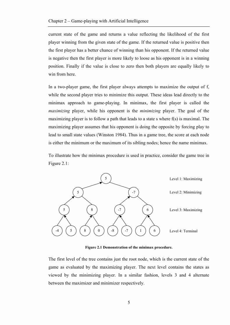
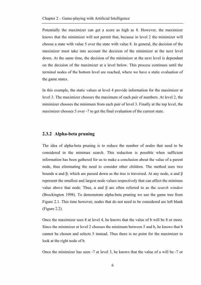
To illustrate how the minimax procedure is used in practice, consider the game tree in
Figure 2.1:
Figure 2.1 Demonstration of the minimax procedure.
The first level of the tree contains just the root node, which is the current state of the
game as evaluated by the maximizing player. The next level contains the states as
viewed by the minimizing player. In a similar fashion, levels 3 and 4 alternate
between the maximizer and minimizer respectively.
5
5 8
-4 5 8 0 61-8 -7
6-7
5 -7
Level 1: Maximizing
Level 4: Terminal
Level 3: Maximizing
Level 2: Minimizing
Chapter 2 – Game-playing with Artificial Intelligence
6
Potentially the maximizer can get a score as high as 8. However, the maximizer
knows that the minimizer will not permit that, because in level 2 the minimizer will
choose a state with value 5 over the state with value 8. In general, the decision of the
maximizer must take into account the decision of the minimizer at the next level
down. At the same time, the decision of the minimizer at the next level is dependant
on the decision of the maximizer at a level below. This process continues until the
terminal nodes of the bottom level are reached, where we have a static evaluation of
the game states.
In this example, the static values at level 4 provide information for the maximizer at
level 3. The maximizer chooses the maximum of each pair of numbers. At level 2, the
minimizer chooses the minimum from each pair of level 3. Finally at the top level, the
maximizer chooses 5 over -7 to get the final evaluation of the current state.
2.3.2 Alpha-beta pruning
The idea of alpha-beta pruning is to reduce the number of nodes that need to be
considered in the minimax search. This reduction is possible when sufficient
information has been gathered for us to make a conclusion about the value of a parent
node, thus eliminating the need to consider other children. The method uses two
bounds α and β, which are passed down as the tree is traversed. At any node, α and β
represent the smallest and largest node values respectively that can affect the minimax
value above that node. Thus, α and β are often referred to as the search window
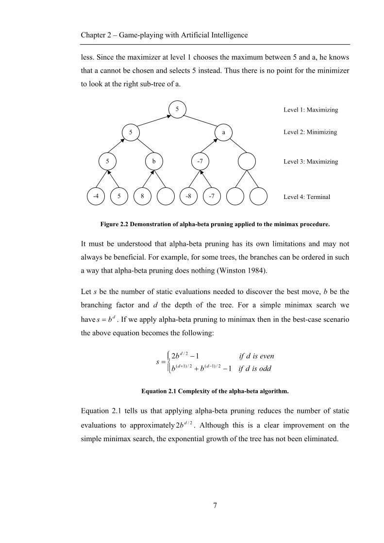
(Brockington 1998). To demonstrate alpha-beta pruning we use the game tree from
Figure 2.1. This time however, nodes that do not need to be considered are left blank
(Figure 2.2).
Once the maximizer sees 8 at level 4, he knows that the value of b will be 8 or more.
Since the minimizer at level 2 chooses the minimum between 5 and b, he knows that b
cannot be chosen and selects 5 instead. Thus there is no point for the maximizer to
look at the right node of b.
Once the minimizer has seen -7 at level 3, he knows that the value of a will be -7 or
Chapter 2 – Game-playing with Artificial Intelligence
7
less. Since the maximizer at level 1 chooses the maximum between 5 and a, he knows
that a cannot be chosen and selects 5 instead. Thus there is no point for the minimizer
to look at the right sub-tree of a.
Figure 2.2 Demonstration of alpha-beta pruning applied to the minimax procedure.
It must be understood that alpha-beta pruning has its own limitations and may not
always be beneficial. For example, for some trees, the branches can be ordered in such
a way that alpha-beta pruning does nothing (Winston 1984).
Let s be the number of static evaluations needed to discover the best move, b be the
branching factor and d the depth of the tree. For a simple minimax search we
have dbs = . If we apply alpha-beta pruning to minimax then in the best-case scenario
the above equation becomes the following:
⎪⎩
⎪⎨⎧
−+
−=
−+ oddisdifbbevenisdifb
sdd
d
112
2/)1(2/)1(
2/
Equation 2.1 Complexity of the alpha-beta algorithm.
Equation 2.1 tells us that applying alpha-beta pruning reduces the number of static
evaluations to approximately 2/2 db . Although this is a clear improvement on the
simple minimax search, the exponential growth of the tree has not been eliminated.
5
5 b
-4 5 8 -8 -7
-7
5 a
Level 1: Maximizing
Level 4: Terminal
Level 3: Maximizing
Level 2: Minimizing
Chapter 2 – Game-playing with Artificial Intelligence
8
2.3.3 Heuristic Pruning
Heuristic methods, like alpha-beta pruning, attempt to reduce the number of static
evaluations needed for a game tree. However, unlike alpha-beta pruning, heuristic
methods do not guarantee to retain the optimal result of a minimax search. Hence
these methods should be used with great caution. It seems obvious that we can reduce
the number of static evaluations by concentrating only on the best moves. Once the
best moves are known we can alter the branching factor so that these moves are
explored further than other moves:
BF(x) = BF(parentOf(x)) – rankOfNode(x)
Equation 2.2 Proposed branching factor for heuristic pruning.
In Equation 2.2 BF(x) is the branching factor for a node x, BF(parentOf(x)) is the
branching factor for the parent node of x and rankOfNode(x) is the rank in plausibility
of the node x among its siblings. For example, if a node is one of seven children and
ranks third most plausible amongst those seven, then it should itself have 7 – 3 = 4
children. This method not only concentrates on the best moves, but also avoids bad
moves, that could potentially lead to disastrous future situations (Winston 1984).
2.3.4 Progressive Deepening
In a tournament environment there are usually bounds set on the time limit allowed for each move. In those situations it may be impractical to search a game tree to a fixed depth, since the search may take too long and no final decision will be made. Progressive deepening is a commonly used technique that combats this problem. As the name suggests, the technique searches the game tree one level at a time, progressively deepening further into the tree. At each new level the best currently available move is recorded. This way, there is always a move available before the time limit is reached (Winston 1984).
Chapter 2 – Game-playing with Artificial Intelligence
9
2.4 Function improvement
As an alternative to search, game-playing systems can be improved by increasing the
accuracy of the board evaluation function. In principle, an ideal board evaluation
function guarantees to provide a correct evaluation for every possible board state, thus
eliminating the need for search. In reality however, such ideal functions can only be
generated for games with small game trees. For all other situations we must rely on
function improvement. There are two main methods by which functions can be
optimised: through natural selection - genetic algorithms and through experience –
Reinforcement Learning.
2.4.1 Genetic Algorithms
Genetic algorithms are well-suited for improving the evaluation function because they
are unlikely to get ‘trapped’ in bad local maxima. This property makes them perfectly
suited for complex domains. Furthermore, they do not depend on gradient information
and perform well where this information is not readily available.
Genetic algorithms have been successfully applied to Checkers (Chellapilla & Fogel
1999, 2001), Othello (Alliot & Durand 1996; Moriarty & Miikkulainen 1995) and
recently to Chess (Fogel et al. 2004). Genetic algorithms operate by evolving a
population of candidate solutions, whose aim is to maximize a given function. The
output of this function is used as a direct measure of the fitness of each candidate
solution. Resembling natural selection, solutions with the highest fitness are chosen.
These chosen solutions are then recombined and mutated to produce the next
generation of candidate solutions. The new candidates compete based on their fitness
with the old candidates for a place in the next generation. This process is repeated
until a sufficiently good candidate is found or until there is no more improvement
between successive generations (Eiben & Smith 2003).
Chapter 2 – Game-playing with Artificial Intelligence
10
2.4.2 Reinforcement Learning
In Reinforcement Learning (RL) the agent learns from its experience. The agent is
rewarded for winning and is punished for losing games. Based on this system, the
agent learns which moves lead to a winning situation and which moves should be
avoided. RL algorithms do not require a complete model of the game, but only its
rules and final outcomes. A popular RL algorithm is Temporal Difference (TD)
learning. In TD, the estimated value of the current board is updated based on the
immediate reward and the estimated value of the subsequent board. In the case of a
deterministic game like Othello, RL algorithms can be extended to learn the values of
subsequent states (afterstates), instead of the usual state-action values. If n states lead
to the same afterstate then by visiting just one of those states, the agent can assign
correct values to all n states (Sutton & Barto 1998).
RL algorithms have been extensively applied to games. The most successful
application was in Backgammon (Tesauro 1992, 1994, 1995), where a program (TD-
Gammon) trained via self-play was able to match top human players. Other
applications include: Chess (Beal & Smith 2000; Dazeley 2001; Thrun 1995),
Connect Four (Ghory 2004), Go (Schraudolph et al. 2000), Othello (Tournavitis 2003;
Walker et al. 1994) and Shogi (Beal & Smith 1999).
Chapter 3 - Reinforcement Learning
11
Chapter 3 Reinforcement Learning
3.1 Introduction
Reinforcement Learning (RL) is a Machine Learning technique, which has become
very popular in recent times. The technique has been applied to a variety of artificial
domains, such as game playing, as well as real-world problems. In principle, a
Reinforcement Learning agent learns from its experience by interacting with the
environment. The agent is not told how to behave and is allowed to explore the
environment freely. However once it has taken its actions, the agent is rewarded if its
actions were good and punished if they were bad. This system of rewards and
punishments teaches the agent which actions to take in the future, and guides it
towards a better outcome.
Usually in RL tasks the agent is not rewarded after each and every action. This creates
what is known as the “temporal credit assignment problem” - when the agent is
eventually awarded, how does it know which actions were most responsible for that
award? Temporal Difference (TD) learning is a RL algorithm that deals with this
problem. In TD learning, the agent learns which states of the environment correlate
highly with rewards, and then uses this knowledge to decide which actions to take.
Reinforcement Learning should not be confused with supervised learning. Unlike in
supervised learning, a Reinforcement Learning agent is not provided with
input/output pairs. Instead, the agent is only given the immediate reward and the next
state. The agent must rely on its experience of possible states, actions, transitions and
rewards to be able to act optimally (Kaelbling et al. 1996).
3.2 History
In the early stages of Artificial Intelligence several researchers began to explore trial-
and-error learning. In 1954, Minsky discussed computational models of
Chapter 3 - Reinforcement Learning
12
Reinforcement Learning. He described the construction of an analog machine
composed of components he called SNARCs (Stochastic Neural Analog
Reinforcement Calculators). Also in 1954, Farley and Clark described a neural-
network learning machine designed to learn by trial and error. In 1960s the terms
"reinforcement" and "reinforcement learning" were used for the first time in literature.
In 1961 Minsky was the first to discuss how to distribute credit among the many
actions that led to a particular goal (credit assignment problem). It is this problem that
the methods of Reinforcement Learning have been trying to solve. In 1968, Michie
and Chambers introduced a Reinforcement Learning controller called BOXES, which
they applied to the pole-balancing task. The pole-balancing task was one of the
earliest tasks involving incomplete knowledge and it soon became the testing ground
for many future RL algorithms. In 1972, Klopf became the first to make a distinction
between supervised and Reinforcement Learning. He argued that supervised methods
prevented the agent from developing adaptive behaviours, which enable it to control
the environment toward desired goals and away from undesired outcomes. Klopf’s
ideas formed the foundation of Reinforcement Learning as we know it today.
3.3 Environment
The agent cannot exist on its own. It must interact with its surroundings by
performing actions and receiving rewards if those actions were deemed appropriate.
In Reinforcement Learning the agent’s surroundings are called the environment.
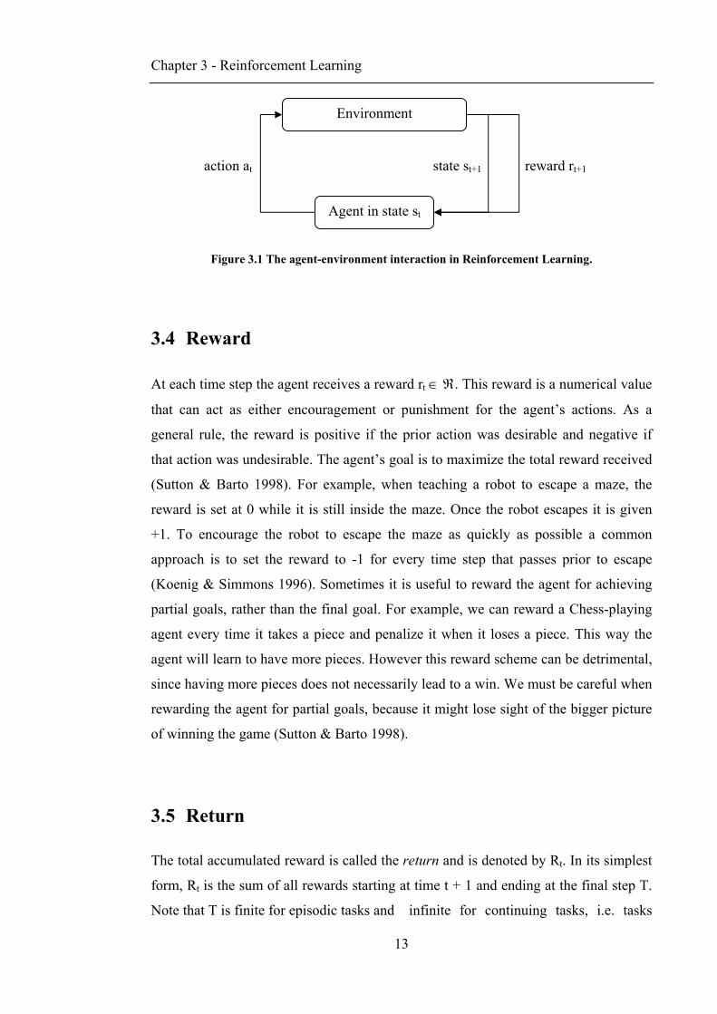
The agent interacts with the environment at each discrete time step t = 0, 1, 2, 3, … At
each time step the agent receives the environment’s representation of the state st from
a set of possible states S. Based on state st, the agent selects an appropriate action at
from a set of available actions for that state A(st). As the consequence of the action at,
the agent receives a reward rt+1 and finds itself at a new state st+1 one time step later
(Sutton & Barto 1998).
Chapter 3 - Reinforcement Learning
13
Figure 3.1 The agent-environment interaction in Reinforcement Learning.
3.4 Reward
At each time step the agent receives a reward rt ∈ ℜ. This reward is a numerical value
that can act as either encouragement or punishment for the agent’s actions. As a
general rule, the reward is positive if the prior action was desirable and negative if
that action was undesirable. The agent’s goal is to maximize the total reward received
(Sutton & Barto 1998). For example, when teaching a robot to escape a maze, the
reward is set at 0 while it is still inside the maze. Once the robot escapes it is given
+1. To encourage the robot to escape the maze as quickly as possible a common
approach is to set the reward to -1 for every time step that passes prior to escape
(Koenig & Simmons 1996). Sometimes it is useful to reward the agent for achieving
partial goals, rather than the final goal. For example, we can reward a Chess-playing
agent every time it takes a piece and penalize it when it loses a piece. This way the
agent will learn to have more pieces. However this reward scheme can be detrimental,
since having more pieces does not necessarily lead to a win. We must be careful when
rewarding the agent for partial goals, because it might lose sight of the bigger picture
of winning the game (Sutton & Barto 1998).
3.5 Return
The total accumulated reward is called the return and is denoted by Rt. In its simplest
form, Rt is the sum of all rewards starting at time t + 1 and ending at the final step T.
Note that T is finite for episodic tasks and infinite for continuing tasks, i.e. tasks
Environment
Agent in state st
action at state st+1 reward rt+1
Chapter 3 - Reinforcement Learning
14
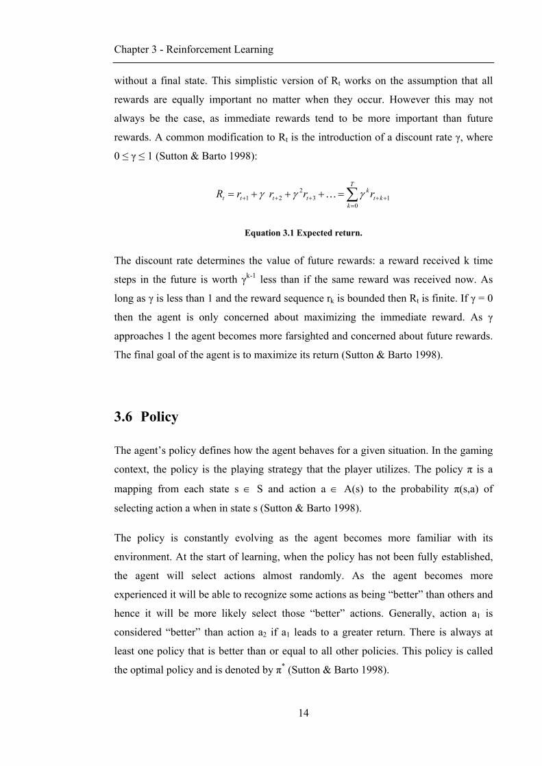
without a final state. This simplistic version of Rt works on the assumption that all
rewards are equally important no matter when they occur. However this may not
always be the case, as immediate rewards tend to be more important than future
rewards. A common modification to Rt is the introduction of a discount rate γ, where
0 ≤ γ ≤ 1 (Sutton & Barto 1998):
∑=
+++++ =+++=T
kkt
ktttt rrrrR
013
221 γγγ K
Equation 3.1 Expected return.
The discount rate determines the value of future rewards: a reward received k time
steps in the future is worth γk-1 less than if the same reward was received now. As
long as γ is less than 1 and the reward sequence rk is bounded then Rt is finite. If γ = 0
then the agent is only concerned about maximizing the immediate reward. As γ
approaches 1 the agent becomes more farsighted and concerned about future rewards.
The final goal of the agent is to maximize its return (Sutton & Barto 1998).
3.6 Policy
The agent’s policy defines how the agent behaves for a given situation. In the gaming
context, the policy is the playing strategy that the player utilizes. The policy π is a
mapping from each state s ∈ S and action a ∈ A(s) to the probability π(s,a) of
selecting action a when in state s (Sutton & Barto 1998).
The policy is constantly evolving as the agent becomes more familiar with its
environment. At the start of learning, when the policy has not been fully established,
the agent will select actions almost randomly. As the agent becomes more
experienced it will be able to recognize some actions as being “better” than others and
hence it will be more likely select those “better” actions. Generally, action a1 is
considered “better” than action a2 if a1 leads to a greater return. There is always at
least one policy that is better than or equal to all other policies. This policy is called
the optimal policy and is denoted by π* (Sutton & Barto 1998).
Chapter 3 - Reinforcement Learning
15
3.7 Exploration and exploitation
An important factor that needs to be considered by a Reinforcement Learning agent is
the balance between exploration and exploitation. In order to obtain rewards the agent
must explore the environment to find states that yield the rewards. At the same time,
the agent would much rather try states that have been rewarding in the past, i.e.
exploit previous knowledge. Exploration and exploitation must go hand in hand for
the agent to be successful. However, the agent must wisely balance their relative
amounts. If there is not enough exploration then there will be a potential goldmine of
unexplored states. On the other hand, insufficient exploitation can lead to a lack of
received reward.
When choosing an action, the agent should not simply select the best available action.
Occasionally it should select a lower ranked exploratory action as it may lead to the
discovery of a better strategy. The following section describes two common
approaches for selecting exploratory actions: ε-greedy and softmax selection.
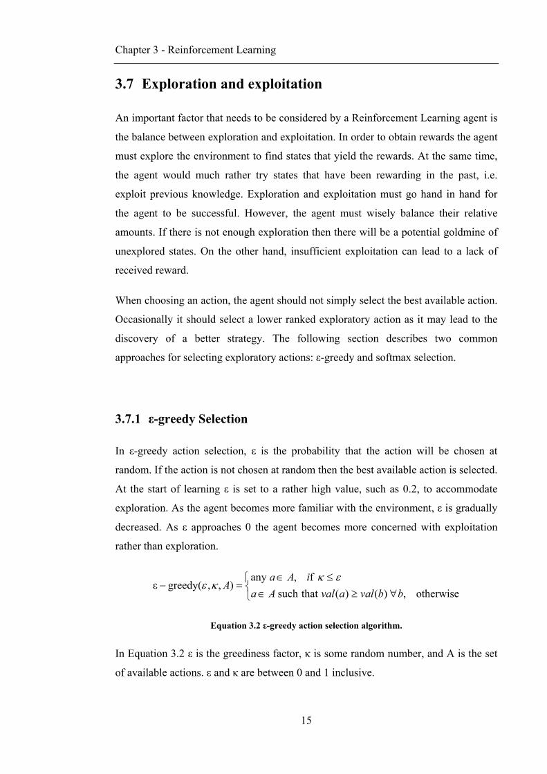
3.7.1 ε-greedy Selection
In ε-greedy action selection, ε is the probability that the action will be chosen at
random. If the action is not chosen at random then the best available action is selected.
At the start of learning ε is set to a rather high value, such as 0.2, to accommodate
exploration. As the agent becomes more familiar with the environment, ε is gradually
decreased. As ε approaches 0 the agent becomes more concerned with exploitation
rather than exploration.
⎩⎨⎧
∀≥∈≤∈
=−otherwise,)()(thatsuch
f,any),,(greedyε
bbvalavalAaiAa
Aεκ
κε
Equation 3.2 ε-greedy action selection algorithm.
In Equation 3.2 ε is the greediness factor, κ is some random number, and A is the set
of available actions. ε and κ are between 0 and 1 inclusive.

Chapter 3 - Reinforcement Learning
16
3.7.2 Softmax Selection
Although ε-greedy is easy to implement it has some major weaknesses. One
disadvantage of ε-greedy is that it can choose an action randomly, even if that action
is completely useless. Choosing the best action as a random choice is not wise either,
as you miss out on the opportunity of exploring the nearly-best actions. It is those
nearly-best actions that may lead to a better policy. Softmax is an action-selection
algorithm that attempts to rectify these problems. Softmax takes into account the
relative values of each action by assuming that they have a Boltzmann distribution.
An action whose value is high has a high probability of being chosen; similarly an
action whose value is low has a low probability of being chosen; finally if two actions
have a similar value then they are both as likely to be chosen. Equation 3.3 gives the
probability of an action being chosen using softmax selection:
∑∈
=
Ai
ival
aval
eeAayprobabilit τ
τ
τ /)(
/)(
),,(
Equation 3.3 Probability of choosing an action a using softmax selection algorithm.
In Equation 3.3 τ is a non-negative value called temperature. The temperature allows
us to control the balance between exploration and exploitation (Wyatt 1997). High
temperatures cause probabilities to be nearly equal, hence promoting exploration. As τ
approaches 0 the probabilities become unevenly distributed making softmax the same
as greedy action selection. In practice the temperature is slowly decayed as shown in
Equation 3.4, so that exploration is favored at the start, while exploitation is preferred
in the later stages of learning.
tkt )0()( ττ =
Equation 3.4 Value of τ at time t. k is the decay constant between 0 and 1.
The temperature decay outlined in Equation 3.4 is far from ideal and can lead to slow
convergence. Some circumstances require the temperature to be manually tuned with
great care (Kaelbling et al. 1996).
Chapter 3 - Reinforcement Learning
17
3.8 Markov Property
A state is called Markov or has the Markov Property if it is able to retain all relevant
information about its past states. For example, we do not require the complete history
of a shuttle cock’s path to predict its future path; it suffices to know its current
direction and speed. It can be shown that if all the past states have the Markov
property then the next state is only dependant on the current state. Iterating this
argument, a prediction that is based solely on the knowledge of the current state is just
as good as a prediction that is based on the knowledge of all the previous states. From
this, it follows that Markov states provide the best possible basis for choosing actions
(Sutton & Barto 1998).
3.9 Markov Decision Processes
A learning task that satisfies the Markov property is called a Markov Decision
Process (MDP). A MDP consists of the following (Kaelbling et al. 1996):
• A set of states S,
• A set of actions A,
• A reward function R: S × A → ℜ, and
• A state transition function T: S × A → Π(S). T(s, a, s’) gives the probability of
making a transition from state s to state s’ using action a.
From the above list we can see that MDPs are important since they can describe the
majority of Reinforcement Learning problems (Sutton & Barto 1998). Given any state
s and action a, the probability of each possible next state s’ is given by:
{ }aassssP ttta
ss ==== + ,|'Pr 1'
Equation 3.5 Probability of the next state in a MDP.
Similarly, given any current state s, action a and any next state s’, the expected value
Chapter 3 - Reinforcement Learning
18
of the next reward is:
{ }',,| 11' ssaassrER ttttass ==== ++
Equation 3.6 Expected value of the next reward in a MDP.
3.10 State-Value Function
A state-value function is a function that estimates the quality of a given state. The
quality of a state is defined in terms of the future rewards that can be expected from
that state. Given that the expected rewards depend on the actions taken by the agent,
the state-value function is defined in terms of the policy used (Sutton & Barto 1998).
The value of a state s under policy π is denoted by Vπ(s) and defined as:
{ }ssREsV tt == |)( ππ
Equation 3.7 State-value function for policy π.
where Eπ denotes the expected value given that the agent follows policy π.
3.11 Action-Value Function
For non-deterministic problems where the outcome state of an action is not known, it
is not sufficient to use the state-value function. For such problems the action-value
function is more appropriate. The action-value function is defined in a similar fashion
to the state-value function (Sutton & Barto 1998). The value of taking action a in state
s under a policy π is denoted by Qπ(s,a) and defined as:
{ }aassREasQ ttt === ,|),( ππ
Equation 3.8 Action-value function for policy π.
Chapter 3 - Reinforcement Learning
19
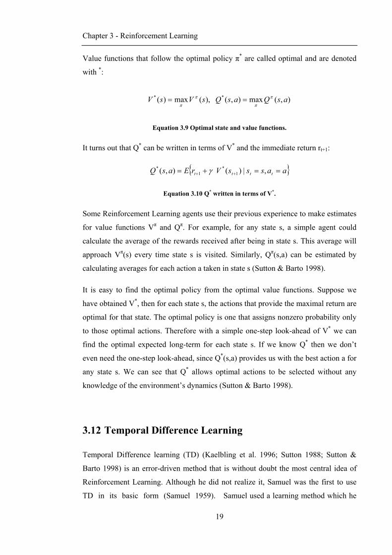
Value functions that follow the optimal policy π* are called optimal and are denoted
with *:
),(max),(),(max)( ** asQasQsVsV π
π
π
π==
Equation 3.9 Optimal state and value functions.
It turns out that Q* can be written in terms of V* and the immediate return rt+1:
{ }aasssVrEasQ tttt ==+= ++ ,|)(),( 1*
1* γ
Equation 3.10 Q* written in terms of V*.
Some Reinforcement Learning agents use their previous experience to make estimates
for value functions Vπ and Qπ. For example, for any state s, a simple agent could
calculate the average of the rewards received after being in state s. This average will
approach Vπ(s) every time state s is visited. Similarly, Qπ(s,a) can be estimated by
calculating averages for each action a taken in state s (Sutton & Barto 1998).
It is easy to find the optimal policy from the optimal value functions. Suppose we
have obtained V*, then for each state s, the actions that provide the maximal return are
optimal for that state. The optimal policy is one that assigns nonzero probability only
to those optimal actions. Therefore with a simple one-step look-ahead of V* we can
find the optimal expected long-term for each state s. If we know Q* then we don’t
even need the one-step look-ahead, since Q*(s,a) provides us with the best action a for
any state s. We can see that Q* allows optimal actions to be selected without any
knowledge of the environment’s dynamics (Sutton & Barto 1998).
3.12 Temporal Difference Learning
Temporal Difference learning (TD) (Kaelbling et al. 1996; Sutton 1988; Sutton &
Barto 1998) is an error-driven method that is without doubt the most central idea of
Reinforcement Learning. Although he did not realize it, Samuel was the first to use
TD in its basic form (Samuel 1959). Samuel used a learning method which he
Chapter 3 - Reinforcement Learning
20
called rote learning. The algorithm saved a description of each board position
encountered together with its backed-up value determined by the minimax search.
This meant, that if a position were to occur again as a terminal position of a search, its
cached value could be used, which in effect amplified the depth of the search. The
algorithm produced slow but continuous improvement that was most effective for
opening and endgame play.
Rote learning ensured that the value of a state is closely related to the values of the
states that follow it - strongly resembling TD learning. In other respects, the algorithm
differs from TD. Samuel’s method uses no rewards and has no special treatment of
terminal positions of the game. In contrast, TD provides rewards or gives a fixed
value to terminal states in order to bind the value function to the true values of the
states (Sutton & Barto 1998).
TD can be tabular, where the value of each state is stored in a table; or applied with
function approximation techniques such as neural networks. In practice however,
tabular TD is only used for simple problems, where the number of states is small and
storing their values is feasible.
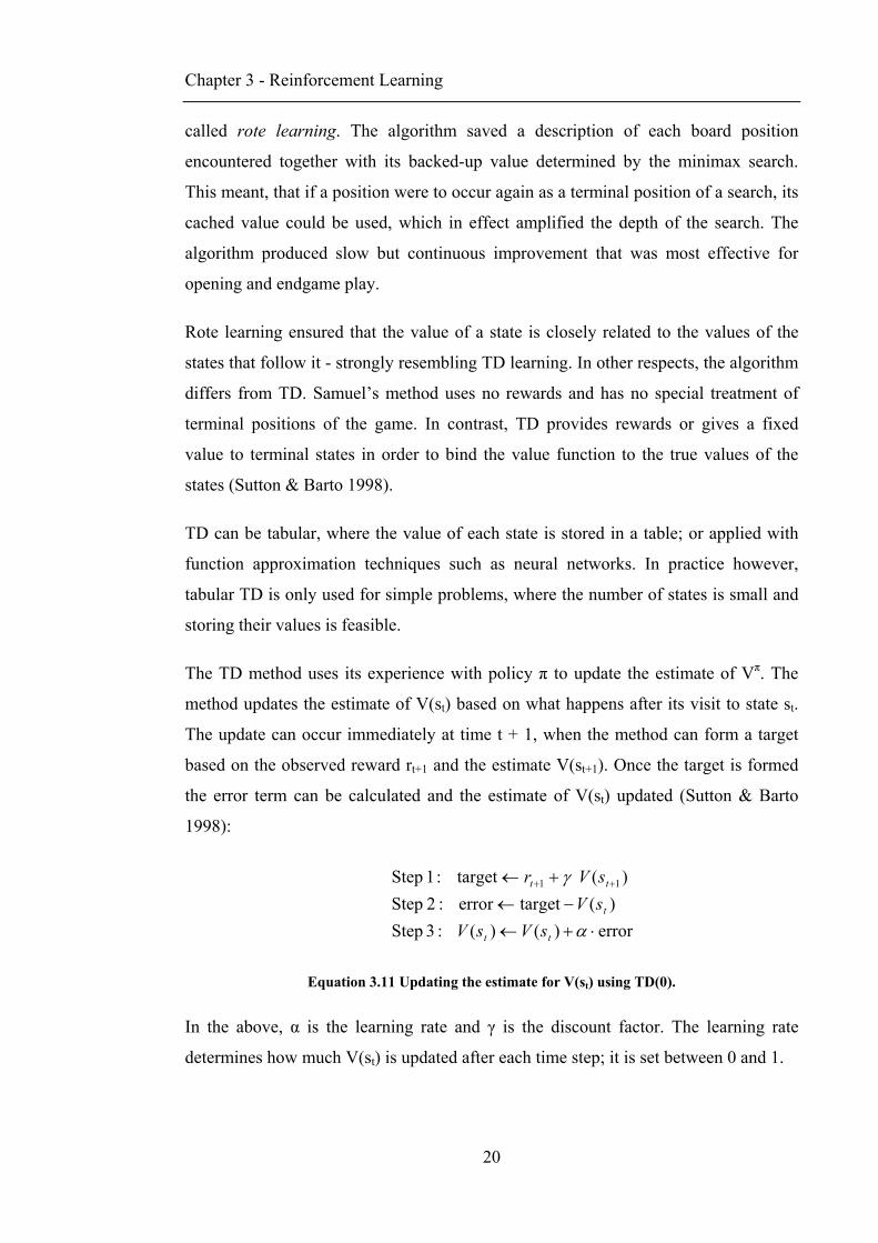
The TD method uses its experience with policy π to update the estimate of Vπ. The
method updates the estimate of V(st) based on what happens after its visit to state st.
The update can occur immediately at time t + 1, when the method can form a target
based on the observed reward rt+1 and the estimate V(st+1). Once the target is formed
the error term can be calculated and the estimate of V(st) updated (Sutton & Barto
1998):
error)()(:3 Step)(targeterror:2 Step
)(target:1Step 11
⋅+←−←
+← ++
α
γ
tt
t
tt
sVsVsVsVr
Equation 3.11 Updating the estimate for V(st) using TD(0).
In the above, α is the learning rate and γ is the discount factor. The learning rate
determines how much V(st) is updated after each time step; it is set between 0 and 1.

Chapter 3 - Reinforcement Learning
21
Figure 3.2 Tabular TD(0) for estimating Vπ.
3.12.1 Advantages of TD methods
TD methods have features that make them well-suited for Reinforcement Learning
tasks (Sutton & Barto 1998):
• They learn estimates based on previous estimates (bootstrap). This makes
learning faster and more accurate.
• They only need to wait one time-step before learning can take place. This is
especially noticeable in tasks with long episodes, where it would be too
inefficient to delay learning until the end of the episode.
• They do not require a model of the environment, its reward and next state
distributions. This is important for dynamic environments whose model is too
hard to compute.
• For any fixed policy π they have been shown to converge to Vπ. In practice,
TD methods have been shown to converge faster than other methods, although
there is no theory to support this.
Initialize V(s) with random values For each learning episode Initialize state s For each step of episode Execute action a given by π for s Observe reward r and next state s’ V(s) ← V(s) + α[r + γV(s’) - V(s)] s ← s’ Until s is terminal
Chapter 3 - Reinforcement Learning
22
3.12.2 Sarsa: On-policy TD algorithm
When it comes to the trade-off between exploration and exploitation, TD algorithms
can be divided into two types: on-policy and off-policy. On-policy algorithms make
no distinction between what is being learned and the policy being followed. These
algorithms treat exploration as part of the policy being learnt. Off-policy algorithms
on the other hand, attempt to learn one strategy (usually the greedy one), while
following a strategy that includes exploratory actions (Sutton & Barto 1998).
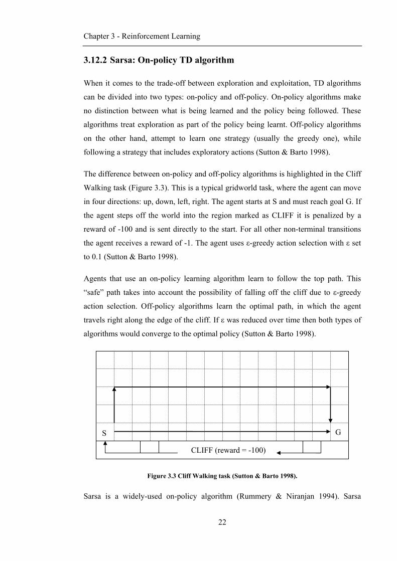
The difference between on-policy and off-policy algorithms is highlighted in the Cliff
Walking task (Figure 3.3). This is a typical gridworld task, where the agent can move
in four directions: up, down, left, right. The agent starts at S and must reach goal G. If
the agent steps off the world into the region marked as CLIFF it is penalized by a
reward of -100 and is sent directly to the start. For all other non-terminal transitions
the agent receives a reward of -1. The agent uses ε-greedy action selection with ε set
to 0.1 (Sutton & Barto 1998).
Agents that use an on-policy learning algorithm learn to follow the top path. This
“safe” path takes into account the possibility of falling off the cliff due to ε-greedy
action selection. Off-policy algorithms learn the optimal path, in which the agent
travels right along the edge of the cliff. If ε was reduced over time then both types of
algorithms would converge to the optimal policy (Sutton & Barto 1998).
Figure 3.3 Cliff Walking task (Sutton & Barto 1998).
Sarsa is a widely-used on-policy algorithm (Rummery & Niranjan 1994). Sarsa
S
CLIFF (reward = -100)
G
Chapter 3 - Reinforcement Learning
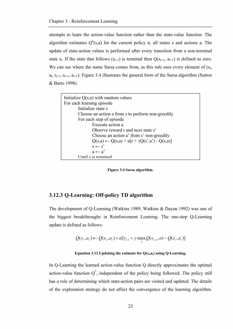
23
attempts to learn the action-value function rather than the state-value function. The
algorithm estimates Qπ(s,a) for the current policy π, all states s and actions a. The
update of state-action values is performed after every transition from a non-terminal
state st. If the state that follows (st+1) is terminal then Q(st+1, at+1) is defined as zero.
We can see where the name Sarsa comes from, as this rule uses every element of (st,
at, rt+1, st+1, at+1). Figure 3.4 illustrates the general form of the Sarsa algorithm (Sutton
& Barto 1998).
Figure 3.4 Sarsa algorithm.
3.12.3 Q-Learning: Off-policy TD algorithm
The development of Q-Learning (Watkins 1989; Watkins & Dayan 1992) was one of
the biggest breakthroughs in Reinforcement Learning. The one-step Q-Learning
update is defined as follows:
)],(),(max[),(),( 11 tttattttt asQasQrasQasQ −++← ++ γα
Equation 3.12 Updating the estimate for Q(st,at) using Q-Learning.
In Q-Learning the learned action-value function Q directly approximates the optimal
action-value function Q*, independent of the policy being followed. The policy still
has a role of determining which state-action pairs are visited and updated. The details
of the exploration strategy do not affect the convergence of the learning algorithm.
Initialize Q(s,a) with random values For each learning episode Initialize state s Choose an action a from s to perform non-greedily For each step of episode Execute action a Observe reward r and next state s’ Choose an action a’ from s’ non-greedily Q(s,a) ← Q(s,a) + α[r + γQ(s’,a’) - Q(s,a)] s ← s’ a ← a’
Until s is terminal
Chapter 3 - Reinforcement Learning
24
For this reason, Q-learning is the most popular algorithm when it comes to learning
from delayed rewards in a model-free environment (Kaelbling et al. 1996).
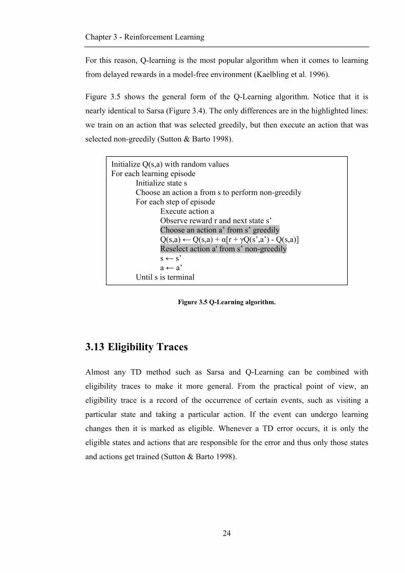
Figure 3.5 shows the general form of the Q-Learning algorithm. Notice that it is
nearly identical to Sarsa (Figure 3.4). The only differences are in the highlighted lines:
we train on an action that was selected greedily, but then execute an action that was
selected non-greedily (Sutton & Barto 1998).
Figure 3.5 Q-Learning algorithm.
3.13 Eligibility Traces
Almost any TD method such as Sarsa and Q-Learning can be combined with
eligibility traces to make it more general. From the practical point of view, an
eligibility trace is a record of the occurrence of certain events, such as visiting a
particular state and taking a particular action. If the event can undergo learning
changes then it is marked as eligible. Whenever a TD error occurs, it is only the
eligible states and actions that are responsible for the error and thus only those states
and actions get trained (Sutton & Barto 1998).
Initialize Q(s,a) with random values For each learning episode Initialize state s Choose an action a from s to perform non-greedily For each step of episode Execute action a Observe reward r and next state s’ Choose an action a’ from s’ greedily Q(s,a) ← Q(s,a) + α[r + γQ(s’,a’) - Q(s,a)]
Reselect action a' from s’ non-greedily s ← s’ a ← a’ Until s is terminal
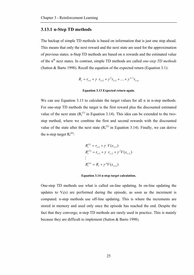
Chapter 3 - Reinforcement Learning
25
3.13.1 n-Step TD methods
The backup of simple TD methods is based on information that is just one step ahead.
This means that only the next reward and the next state are used for the approximation
of previous states. n-Step TD methods are based on n rewards and the estimated value
of the nth next states. In contrast, simple TD methods are called one-step TD methods
(Sutton & Barto 1998). Recall the equation of the expected return (Equation 3.1):
ntn
tttt rrrrR +−
+++ ++++= 13
221 γγγ K
Equation 3.13 Expected return again.
We can use Equation 3.13 to calculate the target values for all n in n-step methods.
For one-step TD methods the target is the first reward plus the discounted estimated
value of the next state (Rt(1) in Equation 3.14). This idea can be extended to the two-
step method, where we combine the first and second rewards with the discounted
value of the state after the next state (Rt(2) in Equation 3.14). Finally, we can derive
the n-step target Rt(n):
)(
)(
)(
)(
22
21)2(
11)1(
ntn
tn
t
tttt
ttt
sVRR
sVrrR
sVrR
+
+++
++
+=
++=
+=
γ
γγ
γ
M
Equation 3.14 n-step target calculation.
One-step TD methods use what is called on-line updating. In on-line updating the
updates to Vt(s) are performed during the episode, as soon as the increment is
computed. n-step methods use off-line updating. This is where the increments are
stored in memory and used only once the episode has reached the end. Despite the
fact that they converge, n-step TD methods are rarely used in practice. This is mainly
because they are difficult to implement (Sutton & Barto 1998).
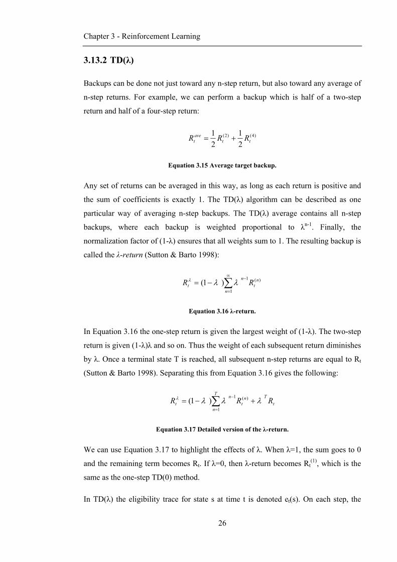
Chapter 3 - Reinforcement Learning
26
3.13.2 TD(λ)
Backups can be done not just toward any n-step return, but also toward any average of
n-step returns. For example, we can perform a backup which is half of a two-step
return and half of a four-step return:
)4()2(
21
21
ttavet RRR +=
Equation 3.15 Average target backup.
Any set of returns can be averaged in this way, as long as each return is positive and
the sum of coefficients is exactly 1. The TD(λ) algorithm can be described as one
particular way of averaging n-step backups. The TD(λ) average contains all n-step
backups, where each backup is weighted proportional to λn-1. Finally, the
normalization factor of (1-λ) ensures that all weights sum to 1. The resulting backup is
called the λ-return (Sutton & Barto 1998):
∑∞
=
−−=
1
)(1)1(n
nt
nt RR λλλ
Equation 3.16 λ-return.
In Equation 3.16 the one-step return is given the largest weight of (1-λ). The two-step
return is given (1-λ)λ and so on. Thus the weight of each subsequent return diminishes
by λ. Once a terminal state T is reached, all subsequent n-step returns are equal to Rt
(Sutton & Barto 1998). Separating this from Equation 3.16 gives the following:
tTn
t
T
n
nt RRR λλλλ +−= ∑
=
− )(
1
1)1(
Equation 3.17 Detailed version of the λ-return.
We can use Equation 3.17 to highlight the effects of λ. When λ=1, the sum goes to 0
and the remaining term becomes Rt. If λ=0, then λ-return becomes Rt(1), which is the
same as the one-step TD(0) method.
In TD(λ) the eligibility trace for state s at time t is denoted et(s). On each step, the
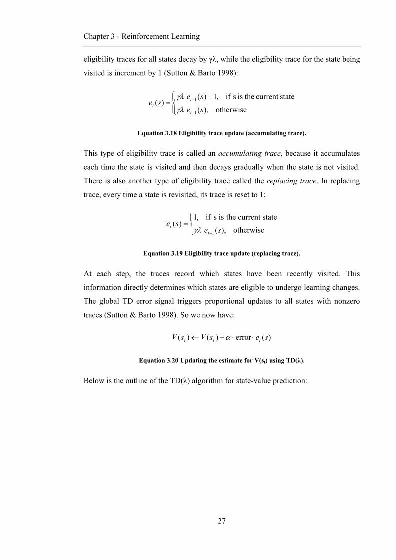
Chapter 3 - Reinforcement Learning
27
eligibility traces for all states decay by γλ, while the eligibility trace for the state being
visited is increment by 1 (Sutton & Barto 1998):
⎪⎩
⎪⎨⎧ +
=−
−
otherwise),(
statecurrent theis s if,1)()(
1
1
se
sese
t
tt γλ
γλ
Equation 3.18 Eligibility trace update (accumulating trace).
This type of eligibility trace is called an accumulating trace, because it accumulates
each time the state is visited and then decays gradually when the state is not visited.
There is also another type of eligibility trace called the replacing trace. In replacing
trace, every time a state is revisited, its trace is reset to 1:
⎩⎨⎧
=− otherwise),(
statecurrenttheissif,1)(
1 sese
tt γλ
Equation 3.19 Eligibility trace update (replacing trace).
At each step, the traces record which states have been recently visited. This
information directly determines which states are eligible to undergo learning changes.
The global TD error signal triggers proportional updates to all states with nonzero
traces (Sutton & Barto 1998). So we now have:
)(error)()( sesVsV ttt ⋅⋅+← α
Equation 3.20 Updating the estimate for V(st) using TD(λ).
Below is the outline of the TD(λ) algorithm for state-value prediction:
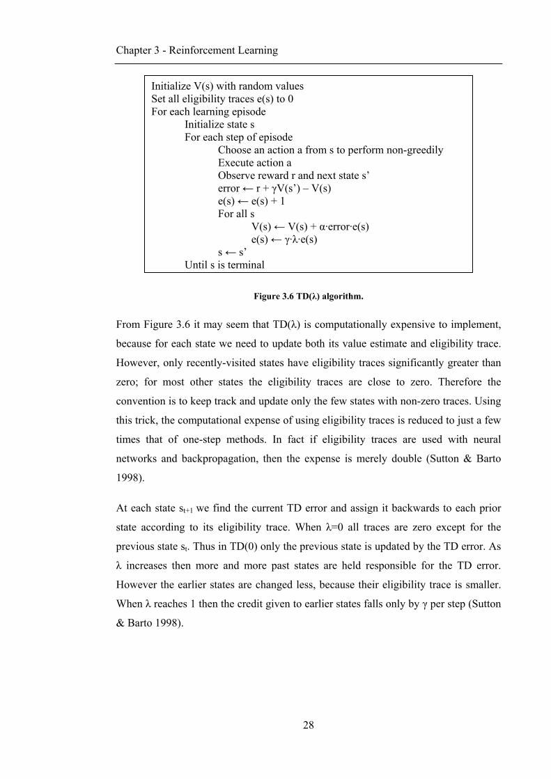
Chapter 3 - Reinforcement Learning
28
Figure 3.6 TD(λ) algorithm.
From Figure 3.6 it may seem that TD(λ) is computationally expensive to implement,
because for each state we need to update both its value estimate and eligibility trace.
However, only recently-visited states have eligibility traces significantly greater than
zero; for most other states the eligibility traces are close to zero. Therefore the
convention is to keep track and update only the few states with non-zero traces. Using
this trick, the computational expense of using eligibility traces is reduced to just a few
times that of one-step methods. In fact if eligibility traces are used with neural
networks and backpropagation, then the expense is merely double (Sutton & Barto
1998).
At each state st+1 we find the current TD error and assign it backwards to each prior
state according to its eligibility trace. When λ=0 all traces are zero except for the
previous state st. Thus in TD(0) only the previous state is updated by the TD error. As
λ increases then more and more past states are held responsible for the TD error.
However the earlier states are changed less, because their eligibility trace is smaller.
When λ reaches 1 then the credit given to earlier states falls only by γ per step (Sutton
& Barto 1998).
Initialize V(s) with random values Set all eligibility traces e(s) to 0 For each learning episode Initialize state s For each step of episode Choose an action a from s to perform non-greedily Execute action a Observe reward r and next state s’ error ← r + γV(s’) – V(s) e(s) ← e(s) + 1 For all s V(s) ← V(s) + α·error·e(s) e(s) ← γ·λ·e(s) s ← s’
Until s is terminal

Chapter 3 - Reinforcement Learning
29
3.14 Function approximation
For most real-world problems it is impossible to store state-values in a look-up-table
because there are simply too many possible states. For example, Othello has a state
space of 1028. For such tasks as Othello, function approximation must be used to
estimate the expected values. One commonly used form of function approximation is
the neural network which is described in detail in the next chapter.
Chapter 4 – Neural Networks
30
Chapter 4 Neural Networks
4.1 Biological Brain
The biological brain is the most powerful piece of ‘machinery’ known to mankind. At
one single point in time, the brain is able to process vast amounts of sensory input,
such as smell, sound, vision, taste and touch, as well as bodily information such as
temperature, pulse and blood pressure. After processing all this information, the brain
must make complex decisions and take appropriate actions by sending control signals
to each and every part of the body.
The brain happens to be one of the most studied organs and yet it is the least
understood. Nevertheless, we are able to describe its operation at a low level. We
know that the brain contains approximately 1010 basic units called neurons, where
each neuron is connected to 104 others (Beale & Jackson 1992).
Just like any machine a neuron accepts a number of inputs. The neuron becomes
activated when enough of these inputs are received at once, otherwise it remains
inactive. The body of the neuron is called the soma (Figure 4.1). The soma is attached
to strands called dendrites. It is through dendrites that the neuron receives inputs. The
dendrites combine inputs similar to a summation method. Another attachment to the
soma is the axon. Unlike the dendrite, the axon is electrically active and serves as the
output channel of the neuron. The axon produces a voltage pulse when a certain
critical threshold is reached. The axon terminates in a special contact called the
synapse (Figure 4.1). The synapse serves as a chemical gate between the axon and the
dendrite of another neuron; opening when its potential is raised enough by the axon’s
voltage pulse. Some synapses excite the dendrite they affect, whilst others serve to
inhibit it. In a mathematical sense, this is equivalent to altering the local potential of
the dendrite from positive to negative respectively (Beale & Jackson 1992).
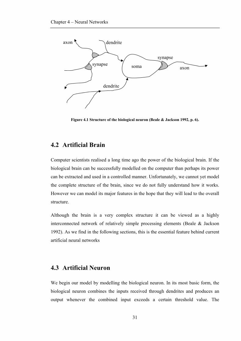
Chapter 4 – Neural Networks
31
Figure 4.1 Structure of the biological neuron (Beale & Jackson 1992, p. 6).
4.2 Artificial Brain
Computer scientists realised a long time ago the power of the biological brain. If the
biological brain can be successfully modelled on the computer than perhaps its power
can be extracted and used in a controlled manner. Unfortunately, we cannot yet model
the complete structure of the brain, since we do not fully understand how it works.
However we can model its major features in the hope that they will lead to the overall
structure.
Although the brain is a very complex structure it can be viewed as a highly
interconnected network of relatively simple processing elements (Beale & Jackson
1992). As we find in the following sections, this is the essential feature behind current
artificial neural networks
4.3 Artificial Neuron
We begin our model by modelling the biological neuron. In its most basic form, the
biological neuron combines the inputs received through dendrites and produces an
output whenever the combined input exceeds a certain threshold value. The
axon soma
axon
dendrite
synapse synapse
dendrite
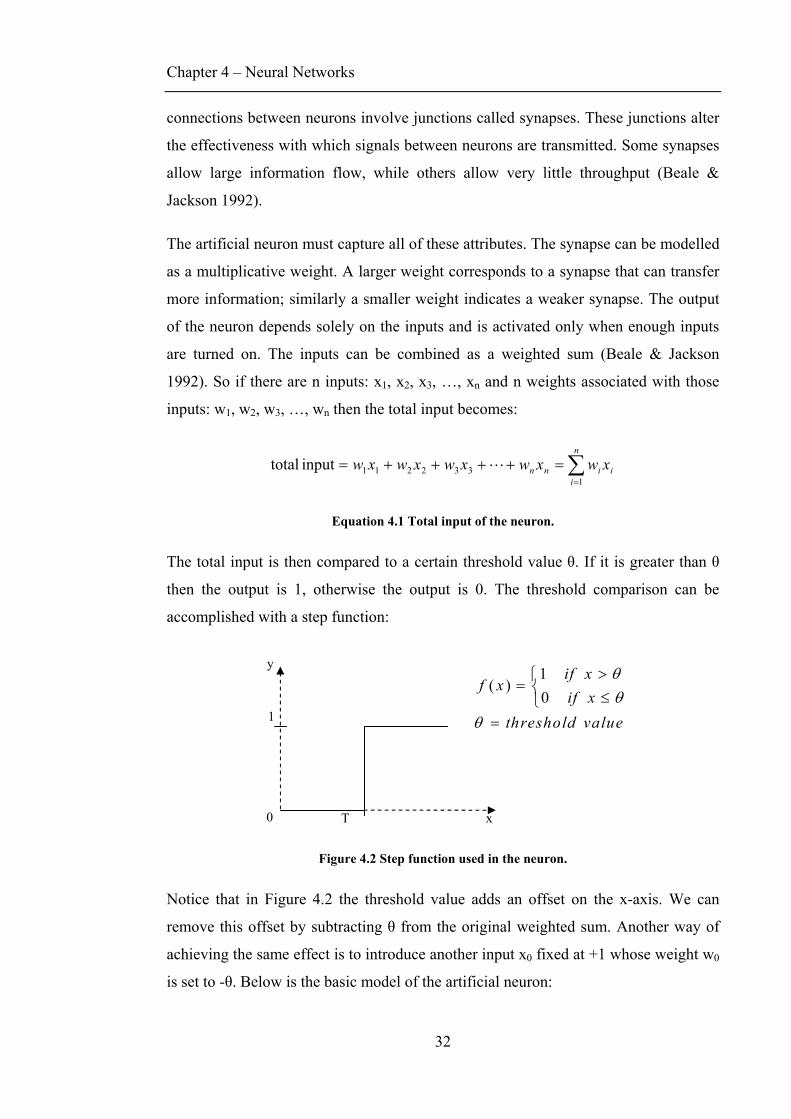
Chapter 4 – Neural Networks
32
connections between neurons involve junctions called synapses. These junctions alter
the effectiveness with which signals between neurons are transmitted. Some synapses
allow large information flow, while others allow very little throughput (Beale &
Jackson 1992).
The artificial neuron must capture all of these attributes. The synapse can be modelled
as a multiplicative weight. A larger weight corresponds to a synapse that can transfer
more information; similarly a smaller weight indicates a weaker synapse. The output
of the neuron depends solely on the inputs and is activated only when enough inputs
are turned on. The inputs can be combined as a weighted sum (Beale & Jackson
1992). So if there are n inputs: x1, x2, x3, …, xn and n weights associated with those
inputs: w1, w2, w3, …, wn then the total input becomes:
∑=
=++++=n
iiinn xwxwxwxwxw
1332211input total L
Equation 4.1 Total input of the neuron.
The total input is then compared to a certain threshold value θ. If it is greater than θ
then the output is 1, otherwise the output is 0. The threshold comparison can be
accomplished with a step function:
Figure 4.2 Step function used in the neuron.
Notice that in Figure 4.2 the threshold value adds an offset on the x-axis. We can
remove this offset by subtracting θ from the original weighted sum. Another way of
achieving the same effect is to introduce another input x0 fixed at +1 whose weight w0
is set to -θ. Below is the basic model of the artificial neuron:
0
1
y
xT
valuethresholdxifxif
xf
=⎩⎨⎧
≤>
=
θθθ
01
)(
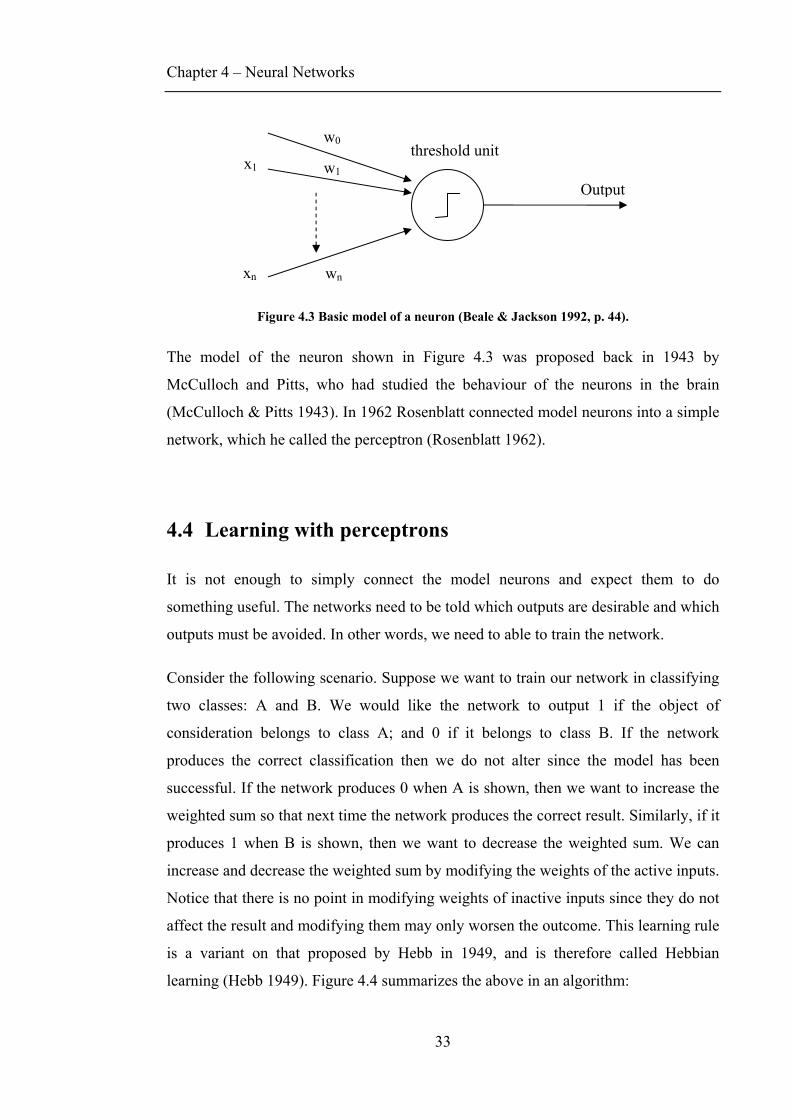
Chapter 4 – Neural Networks
33
Figure 4.3 Basic model of a neuron (Beale & Jackson 1992, p. 44).
The model of the neuron shown in Figure 4.3 was proposed back in 1943 by
McCulloch and Pitts, who had studied the behaviour of the neurons in the brain
(McCulloch & Pitts 1943). In 1962 Rosenblatt connected model neurons into a simple
network, which he called the perceptron (Rosenblatt 1962).
4.4 Learning with perceptrons
It is not enough to simply connect the model neurons and expect them to do
something useful. The networks need to be told which outputs are desirable and which
outputs must be avoided. In other words, we need to able to train the network.
Consider the following scenario. Suppose we want to train our network in classifying
two classes: A and B. We would like the network to output 1 if the object of
consideration belongs to class A; and 0 if it belongs to class B. If the network
produces the correct classification then we do not alter since the model has been
successful. If the network produces 0 when A is shown, then we want to increase the
weighted sum so that next time the network produces the correct result. Similarly, if it
produces 1 when B is shown, then we want to decrease the weighted sum. We can
increase and decrease the weighted sum by modifying the weights of the active inputs.
Notice that there is no point in modifying weights of inactive inputs since they do not
affect the result and modifying them may only worsen the outcome. This learning rule
is a variant on that proposed by Hebb in 1949, and is therefore called Hebbian
learning (Hebb 1949). Figure 4.4 summarizes the above in an algorithm:
wn
Output
threshold unit
x1
w0
w1
xn
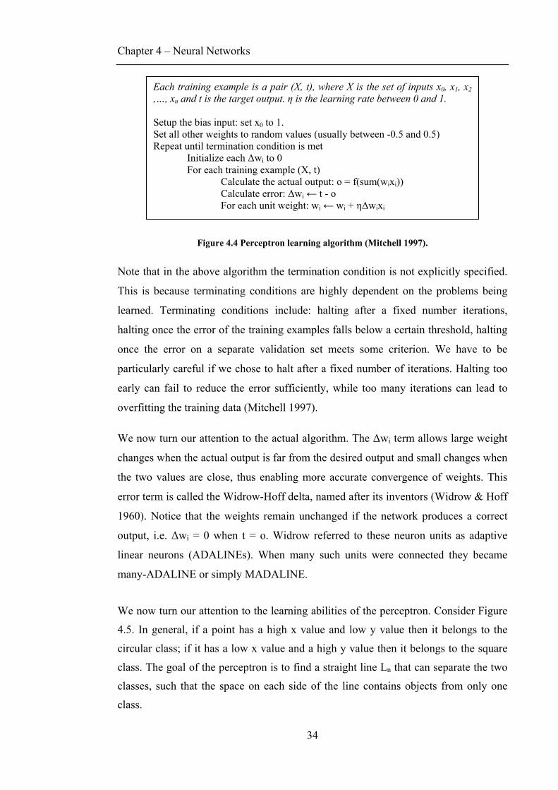
Chapter 4 – Neural Networks
34
Figure 4.4 Perceptron learning algorithm (Mitchell 1997).
Note that in the above algorithm the termination condition is not explicitly specified.
This is because terminating conditions are highly dependent on the problems being
learned. Terminating conditions include: halting after a fixed number iterations,
halting once the error of the training examples falls below a certain threshold, halting
once the error on a separate validation set meets some criterion. We have to be
particularly careful if we chose to halt after a fixed number of iterations. Halting too
early can fail to reduce the error sufficiently, while too many iterations can lead to
overfitting the training data (Mitchell 1997).
We now turn our attention to the actual algorithm. The Δwi term allows large weight
changes when the actual output is far from the desired output and small changes when
the two values are close, thus enabling more accurate convergence of weights. This
error term is called the Widrow-Hoff delta, named after its inventors (Widrow & Hoff
1960). Notice that the weights remain unchanged if the network produces a correct
output, i.e. Δwi = 0 when t = o. Widrow referred to these neuron units as adaptive
linear neurons (ADALINEs). When many such units were connected they became
many-ADALINE or simply MADALINE.
We now turn our attention to the learning abilities of the perceptron. Consider Figure
4.5. In general, if a point has a high x value and low y value then it belongs to the
circular class; if it has a low x value and a high y value then it belongs to the square
class. The goal of the perceptron is to find a straight line Ln that can separate the two
classes, such that the space on each side of the line contains objects from only one
class.
Each training example is a pair (X, t), where X is the set of inputs x0, x1, x2,…, xn and t is the target output. η is the learning rate between 0 and 1. Setup the bias input: set x0 to 1. Set all other weights to random values (usually between -0.5 and 0.5) Repeat until termination condition is met Initialize each Δwi to 0
For each training example (X, t) Calculate the actual output: o = f(sum(wixi)) Calculate error: Δwi ← t - o For each unit weight: wi ← wi + ηΔwixi
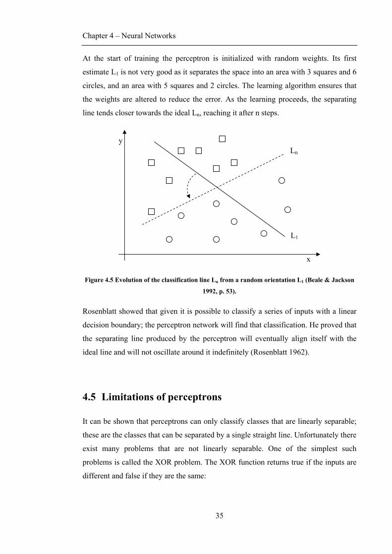
Chapter 4 – Neural Networks
35
At the start of training the perceptron is initialized with random weights. Its first
estimate L1 is not very good as it separates the space into an area with 3 squares and 6
circles, and an area with 5 squares and 2 circles. The learning algorithm ensures that
the weights are altered to reduce the error. As the learning proceeds, the separating
line tends closer towards the ideal Ln, reaching it after n steps.
Figure 4.5 Evolution of the classification line Ln from a random orientation L1 (Beale & Jackson
1992, p. 53).
Rosenblatt showed that given it is possible to classify a series of inputs with a linear
decision boundary; the perceptron network will find that classification. He proved that
the separating line produced by the perceptron will eventually align itself with the
ideal line and will not oscillate around it indefinitely (Rosenblatt 1962).
4.5 Limitations of perceptrons
It can be shown that perceptrons can only classify classes that are linearly separable;
these are the classes that can be separated by a single straight line. Unfortunately there
exist many problems that are not linearly separable. One of the simplest such
problems is called the XOR problem. The XOR function returns true if the inputs are
different and false if they are the same:
x
Ln
L1
y

Chapter 4 – Neural Networks
36
A B A XOR B
False False False
False True True
True False True
True True False
Table 4.1 XOR logical function.
Consider the graphical representation of the XOR problem (Figure 4.6). Clearly it is
not possible to draw a single straight line that separates squares from circles.
Therefore the perceptron will not be able to solve this problem, or any such linearly
inseparable problem. This fact, demonstrated by Minsky and Papert in 1969, was
regarded as a mortal blow to the area of neural networks (Minsky & Papert 1969). As
a result, the majority of the scientific community gave up on the idea and moved on to
more promising areas (Beale & Jackson 1992).
Figure 4.6 Graphical representation of the XOR problem.
4.6 Multilayer Perceptron
Minsky and Papert showed that the key to solving the XOR problem lies in using
B
True
False
True A False
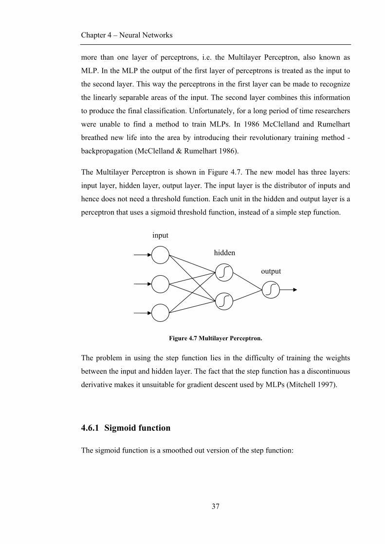
Chapter 4 – Neural Networks
37
more than one layer of perceptrons, i.e. the Multilayer Perceptron, also known as
MLP. In the MLP the output of the first layer of perceptrons is treated as the input to
the second layer. This way the perceptrons in the first layer can be made to recognize
the linearly separable areas of the input. The second layer combines this information
to produce the final classification. Unfortunately, for a long period of time researchers
were unable to find a method to train MLPs. In 1986 McClelland and Rumelhart
breathed new life into the area by introducing their revolutionary training method -
backpropagation (McClelland & Rumelhart 1986).
The Multilayer Perceptron is shown in Figure 4.7. The new model has three layers:
input layer, hidden layer, output layer. The input layer is the distributor of inputs and
hence does not need a threshold function. Each unit in the hidden and output layer is a
perceptron that uses a sigmoid threshold function, instead of a simple step function.
Figure 4.7 Multilayer Perceptron.
The problem in using the step function lies in the difficulty of training the weights
between the input and hidden layer. The fact that the step function has a discontinuous
derivative makes it unsuitable for gradient descent used by MLPs (Mitchell 1997).
4.6.1 Sigmoid function
The sigmoid function is a smoothed out version of the step function:
input
hidden
output
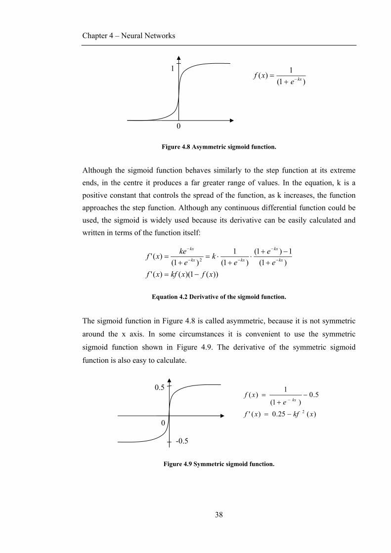
Chapter 4 – Neural Networks
38
Figure 4.8 Asymmetric sigmoid function.
Although the sigmoid function behaves similarly to the step function at its extreme ends, in the centre it produces a far greater range of values. In the equation, k is a positive constant that controls the spread of the function, as k increases, the function approaches the step function. Although any continuous differential function could be used, the sigmoid is widely used because its derivative can be easily calculated and written in terms of the function itself:
))(1)(()(')1(
1)1()1(
1)1(
)(' 2
xfxkfxfe
ee
ke
kexf kx
kx
kxkx
kx
−=+
−+⋅
+⋅=
+= −
−
−−
−
Equation 4.2 Derivative of the sigmoid function.
The sigmoid function in Figure 4.8 is called asymmetric, because it is not symmetric
around the x axis. In some circumstances it is convenient to use the symmetric
sigmoid function shown in Figure 4.9. The derivative of the symmetric sigmoid
function is also easy to calculate.
Figure 4.9 Symmetric sigmoid function.
)(25.0)('
5.0)1(
1)(
2 xkfxfe
xfkx
−=
−+
=−
0
0.5
0
)1(1)( kxe
xf −+=
1
-0.5
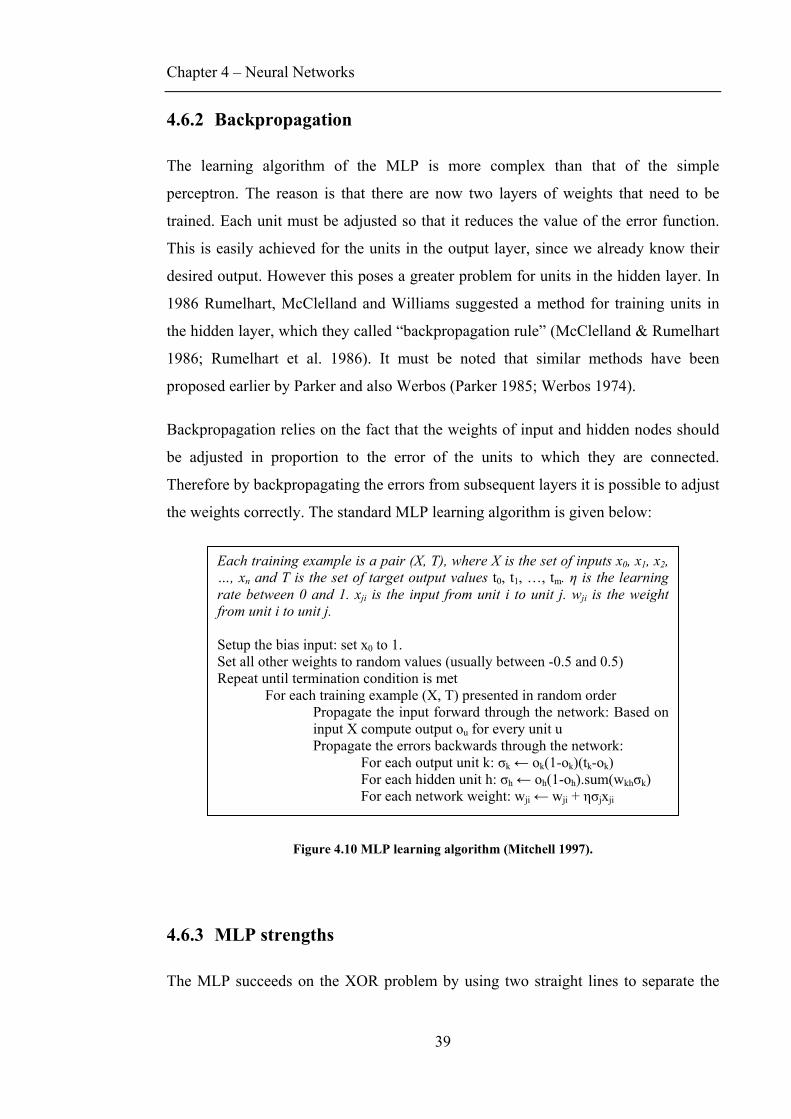
Chapter 4 – Neural Networks
39
4.6.2 Backpropagation
The learning algorithm of the MLP is more complex than that of the simple
perceptron. The reason is that there are now two layers of weights that need to be
trained. Each unit must be adjusted so that it reduces the value of the error function.
This is easily achieved for the units in the output layer, since we already know their
desired output. However this poses a greater problem for units in the hidden layer. In
1986 Rumelhart, McClelland and Williams suggested a method for training units in
the hidden layer, which they called “backpropagation rule” (McClelland & Rumelhart
1986; Rumelhart et al. 1986). It must be noted that similar methods have been
proposed earlier by Parker and also Werbos (Parker 1985; Werbos 1974).
Backpropagation relies on the fact that the weights of input and hidden nodes should
be adjusted in proportion to the error of the units to which they are connected.
Therefore by backpropagating the errors from subsequent layers it is possible to adjust
the weights correctly. The standard MLP learning algorithm is given below:
Figure 4.10 MLP learning algorithm (Mitchell 1997).
4.6.3 MLP strengths
The MLP succeeds on the XOR problem by using two straight lines to separate the
Each training example is a pair (X, T), where X is the set of inputs x0, x1, x2, …, xn and T is the set of target output values t0, t1, …, tm. η is the learning rate between 0 and 1. xji is the input from unit i to unit j. wji is the weight from unit i to unit j. Setup the bias input: set x0 to 1. Set all other weights to random values (usually between -0.5 and 0.5) Repeat until termination condition is met
For each training example (X, T) presented in random order Propagate the input forward through the network: Based on input X compute output ou for every unit u Propagate the errors backwards through the network: For each output unit k: σk ← ok(1-ok)(tk-ok) For each hidden unit h: σh ← oh(1-oh).sum(wkhσk) For each network weight: wji ← wji + ησjxji
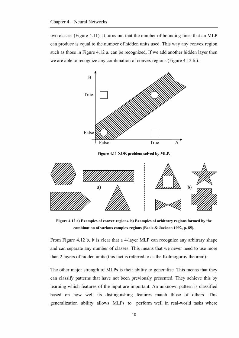
Chapter 4 – Neural Networks
40
two classes (Figure 4.11). It turns out that the number of bounding lines that an MLP
can produce is equal to the number of hidden units used. This way any convex region
such as those in Figure 4.12 a. can be recognized. If we add another hidden layer then
we are able to recognize any combination of convex regions (Figure 4.12 b.).
Figure 4.11 XOR problem solved by MLP.
Figure 4.12 a) Examples of convex regions. b) Examples of arbitrary regions formed by the
combination of various complex regions (Beale & Jackson 1992, p. 85).
From Figure 4.12 b. it is clear that a 4-layer MLP can recognize any arbitrary shape
and can separate any number of classes. This means that we never need to use more
than 2 layers of hidden units (this fact is referred to as the Kolmogorov theorem).
The other major strength of MLPs is their ability to generalize. This means that they
can classify patterns that have not been previously presented. They achieve this by
learning which features of the input are important. An unknown pattern is classified
based on how well its distinguishing features match those of others. This
generalization ability allows MLPs to perform well in real-world tasks where
True
False
TrueFalse A
B
a) b)
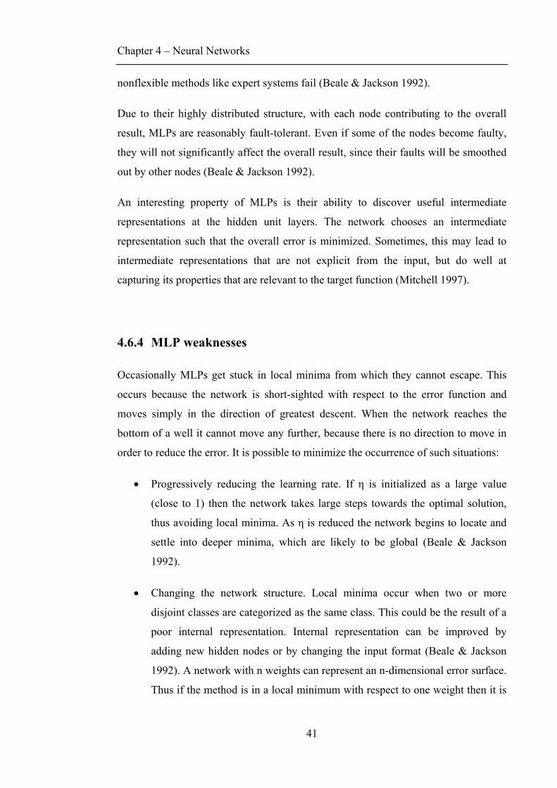
Chapter 4 – Neural Networks
41
nonflexible methods like expert systems fail (Beale & Jackson 1992).
Due to their highly distributed structure, with each node contributing to the overall
result, MLPs are reasonably fault-tolerant. Even if some of the nodes become faulty,
they will not significantly affect the overall result, since their faults will be smoothed
out by other nodes (Beale & Jackson 1992).
An interesting property of MLPs is their ability to discover useful intermediate
representations at the hidden unit layers. The network chooses an intermediate
representation such that the overall error is minimized. Sometimes, this may lead to
intermediate representations that are not explicit from the input, but do well at
capturing its properties that are relevant to the target function (Mitchell 1997).
4.6.4 MLP weaknesses
Occasionally MLPs get stuck in local minima from which they cannot escape. This
occurs because the network is short-sighted with respect to the error function and
moves simply in the direction of greatest descent. When the network reaches the
bottom of a well it cannot move any further, because there is no direction to move in
order to reduce the error. It is possible to minimize the occurrence of such situations:
• Progressively reducing the learning rate. If η is initialized as a large value
(close to 1) then the network takes large steps towards the optimal solution,
thus avoiding local minima. As η is reduced the network begins to locate and
settle into deeper minima, which are likely to be global (Beale & Jackson
1992).
• Changing the network structure. Local minima occur when two or more
disjoint classes are categorized as the same class. This could be the result of a
poor internal representation. Internal representation can be improved by
adding new hidden nodes or by changing the input format (Beale & Jackson
1992). A network with n weights can represent an n-dimensional error surface.
Thus if the method is in a local minimum with respect to one weight then it is
Chapter 4 – Neural Networks
42
not necessarily in a local minimum with respect to other weights. So, addition
of a weight acts as an extra escape route for the gradient descent algorithm
(Mitchell 1997).
• Introducing the momentum term α. The effect of α is to produce large changes
in weight if the previous changes have been large, and small changes if they
have been small. Momentum can also speed up convergence along shallow
gradients (Beale & Jackson 1992).
• Adding noise to the input. Random noise can cause the gradient descent
algorithm to circumvent the path of steepest descent, which is often enough to
escape from a local minimum. This approach is simple and does not
noticeably slow down the gradient descent algorithm (Beale & Jackson 1992).
• Train multiple networks with different random weights for the same data set.
This is likely to lead to produce networks with varying levels of ability. We
can then use the network with the best ability. Alternatively, we can combine
those networks to form what is known as an ensemble. The output of an
ensemble can be either the average of the individual network outputs or based
on some kind of a voting system (Mitchell 1997).
Whilst strong at generalisation, MLPs are not so good at extrapolation. When given
an unseen pattern that is a mixture of previously classified patterns, the network tends
to classify it as an example of the predominant pattern (Mitchell 1997).
One other problem with MLPs is their slow convergence rate. The networks require
many iterations through the same set of input patterns before they are able to settle
into a stable solution. This is especially the case in problems with a complex error
surface. There are ways of improving convergence rates, such as the addition of the
momentum term. Another method is to increase the learning rate η. Finally, it is also
possible to use the second order derivative of the gradient, which increases the
accuracy of the descent. However, this involves additional computational expenses
and is therefore rarely used in practice (Beale & Jackson 1992).
Chapter 4 – Neural Networks
43
4.7 Constructive Architecture
Constructive neural networks differ from MLPs in two significant ways. First of all
they have a constructive architecture in which the hidden nodes are not fixed, but are
added one at a time as the network learns. Such hidden units respond only to a local
region of the input space. Secondly, they have a different learning algorithm in which
only one hidden unit is trained at one time. These networks can form compact input
representations, while learning easily and rapidly. Constructive neural networks can
be divided into two categories based on the activation function of their hidden
neurons. Cascade networks use global activation functions, while resource-allocating
networks have local responsive activation functions (Vamplew & Ollington 2005b).
Various cascade-style networks have been developed: Cascade-Correlation, Modified
Cascade-Correlation, Cascade and Cascade Network (Lahnajarvi et al. 2002). Based
on the findings by Lahnajarvi et al., Cascade-Correlation outperforms all other
cascade networks on 5 of the 10 benchmark classification and regression tasks. For
the purpose of this thesis, Cascade2 has been used, which is a variation of Cascade-
Correlation.
4.7.1 Cascade-Correlation
Cascade-Correlation or simply Cascor networks receive their name due to the cascade
architecture and the fact that each new hidden node attempts to maximize the
correlation between itself and the residual error signal (Fahlman & Lebiere 1990).
The network begins with some predefined number of inputs and output, but no hidden
units. All the inputs (including the bias) are connected to the outputs. The output units
can use either a linear or a sigmoidal activation function (Fahlman & Lebiere 1990).
The cascading architecture removes the need for backpropagation and hence the units
can be trained with the standard perceptron learning algorithm. Cascor usually uses
the Quickprop algorithm (Fahlman 1988). Just like backpropagation Quickprop
computes partial derivatives, but instead of using gradient descent it updates weights
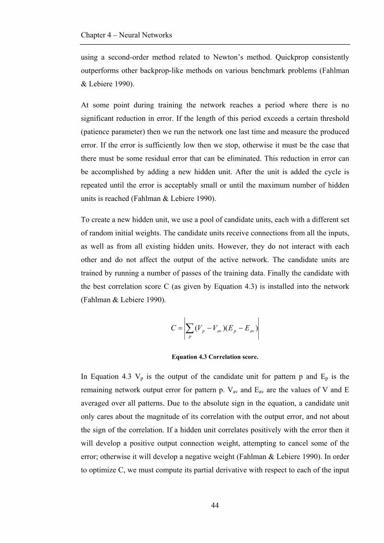
Chapter 4 – Neural Networks
44
using a second-order method related to Newton’s method. Quickprop consistently
outperforms other backprop-like methods on various benchmark problems (Fahlman
& Lebiere 1990).
At some point during training the network reaches a period where there is no
significant reduction in error. If the length of this period exceeds a certain threshold
(patience parameter) then we run the network one last time and measure the produced
error. If the error is sufficiently low then we stop, otherwise it must be the case that
there must be some residual error that can be eliminated. This reduction in error can
be accomplished by adding a new hidden unit. After the unit is added the cycle is
repeated until the error is acceptably small or until the maximum number of hidden
units is reached (Fahlman & Lebiere 1990).
To create a new hidden unit, we use a pool of candidate units, each with a different set
of random initial weights. The candidate units receive connections from all the inputs,
as well as from all existing hidden units. However, they do not interact with each
other and do not affect the output of the active network. The candidate units are
trained by running a number of passes of the training data. Finally the candidate with
the best correlation score C (as given by Equation 4.3) is installed into the network
(Fahlman & Lebiere 1990).
∑ −−=p
avpavp EEVVC ))((
Equation 4.3 Correlation score.
In Equation 4.3 Vp is the output of the candidate unit for pattern p and Ep is the
remaining network output error for pattern p. Vav and Eav are the values of V and E
averaged over all patterns. Due to the absolute sign in the equation, a candidate unit
only cares about the magnitude of its correlation with the output error, and not about
the sign of the correlation. If a hidden unit correlates positively with the error then it
will develop a positive output connection weight, attempting to cancel some of the
error; otherwise it will develop a negative weight (Fahlman & Lebiere 1990). In order
to optimize C, we must compute its partial derivative with respect to each of the input
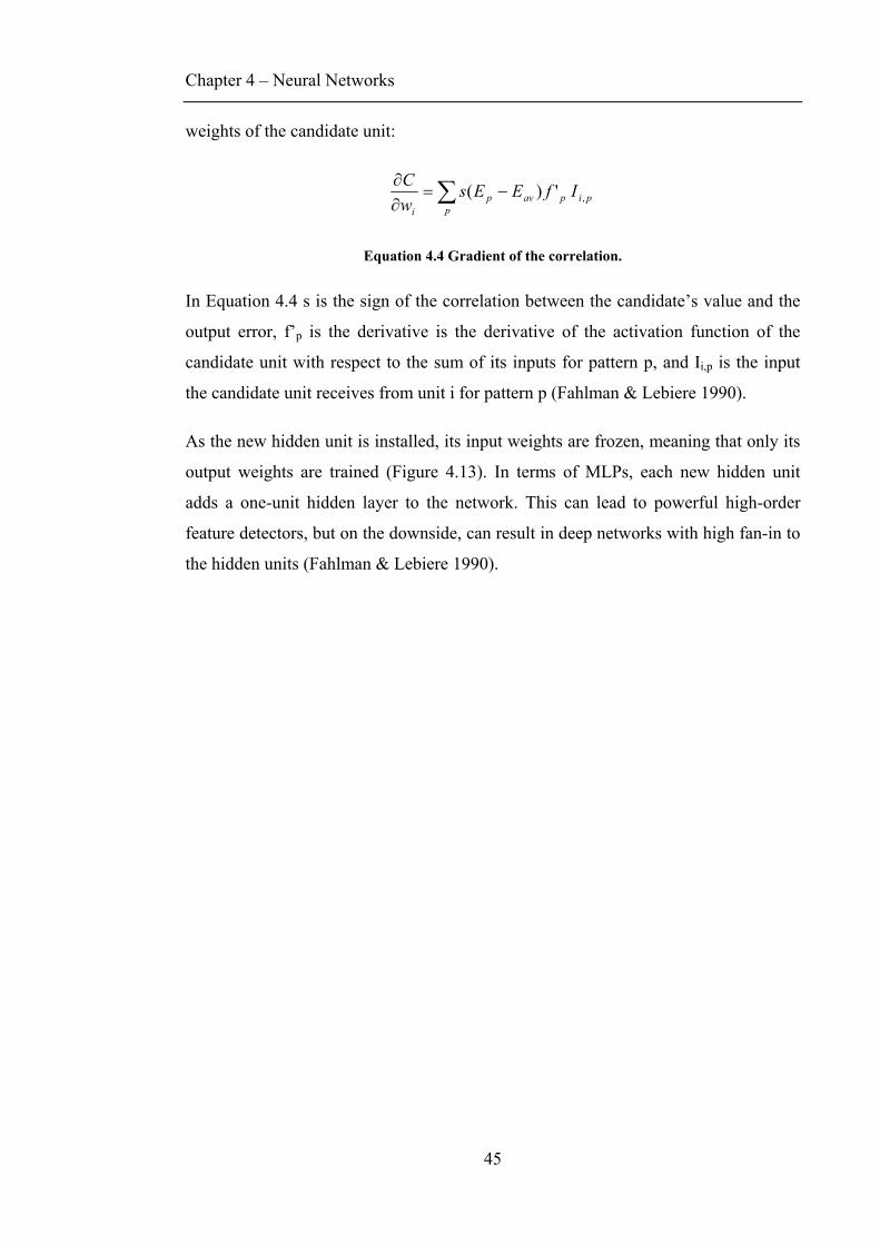
Chapter 4 – Neural Networks
45
weights of the candidate unit:
∑ −=∂∂
ppipavp
i
IfEEswC
,')(
Equation 4.4 Gradient of the correlation.
In Equation 4.4 s is the sign of the correlation between the candidate’s value and the
output error, f’p is the derivative is the derivative of the activation function of the
candidate unit with respect to the sum of its inputs for pattern p, and Ii,p is the input
the candidate unit receives from unit i for pattern p (Fahlman & Lebiere 1990).
As the new hidden unit is installed, its input weights are frozen, meaning that only its
output weights are trained (Figure 4.13). In terms of MLPs, each new hidden unit
adds a one-unit hidden layer to the network. This can lead to powerful high-order
feature detectors, but on the downside, can result in deep networks with high fan-in to
the hidden units (Fahlman & Lebiere 1990).
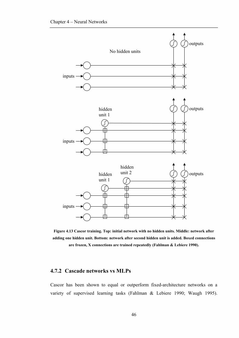
Chapter 4 – Neural Networks
46
Figure 4.13 Cascor training. Top: initial network with no hidden units. Middle: network after
adding one hidden unit. Bottom: network after second hidden unit is added. Boxed connections
are frozen, X connections are trained repeatedly (Fahlman & Lebiere 1990).
4.7.2 Cascade networks vs MLPs
Cascor has been shown to equal or outperform fixed-architecture networks on a
variety of supervised learning tasks (Fahlman & Lebiere 1990; Waugh 1995).
inputs
outputs
inputs
outputs hidden unit 1
inputs
outputs hidden unit 1
hidden unit 2
No hidden units
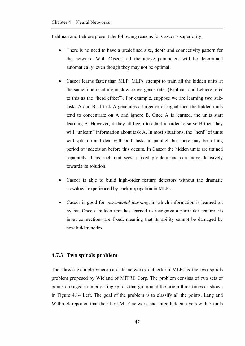
Chapter 4 – Neural Networks
47
Fahlman and Lebiere present the following reasons for Cascor’s superiority:
• There is no need to have a predefined size, depth and connectivity pattern for
the network. With Cascor, all the above parameters will be determined
automatically, even though they may not be optimal.
• Cascor learns faster than MLP. MLPs attempt to train all the hidden units at
the same time resulting in slow convergence rates (Fahlman and Lebiere refer
to this as the “herd effect”). For example, suppose we are learning two sub-
tasks A and B. If task A generates a larger error signal then the hidden units
tend to concentrate on A and ignore B. Once A is learned, the units start
learning B. However, if they all begin to adapt in order to solve B then they
will “unlearn” information about task A. In most situations, the “herd” of units
will split up and deal with both tasks in parallel, but there may be a long
period of indecision before this occurs. In Cascor the hidden units are trained
separately. Thus each unit sees a fixed problem and can move decisively
towards its solution.
• Cascor is able to build high-order feature detectors without the dramatic
slowdown experienced by backpropagation in MLPs.
• Cascor is good for incremental learning, in which information is learned bit
by bit. Once a hidden unit has learned to recognize a particular feature, its
input connections are fixed, meaning that its ability cannot be damaged by
new hidden nodes.
4.7.3 Two spirals problem
The classic example where cascade networks outperform MLPs is the two spirals
problem proposed by Wieland of MITRE Corp. The problem consists of two sets of
points arranged in interlocking spirals that go around the origin three times as shown
in Figure 4.14 Left. The goal of the problem is to classify all the points. Lang and
Witbrock reported that their best MLP network had three hidden layers with 5 units
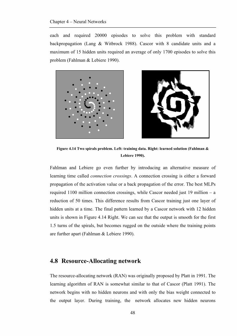
Chapter 4 – Neural Networks
48
each and required 20000 episodes to solve this problem with standard
backpropagation (Lang & Witbrock 1988). Cascor with 8 candidate units and a
maximum of 15 hidden units required an average of only 1700 episodes to solve this
problem (Fahlman & Lebiere 1990).
Figure 4.14 Two spirals problem. Left: training data. Right: learned solution (Fahlman &
Lebiere 1990).
Fahlman and Lebiere go even further by introducing an alternative measure of
learning time called connection crossings. A connection crossing is either a forward
propagation of the activation value or a back propagation of the error. The best MLPs
required 1100 million connection crossings, while Cascor needed just 19 million – a
reduction of 50 times. This difference results from Cascor training just one layer of
hidden units at a time. The final pattern learned by a Cascor network with 12 hidden
units is shown in Figure 4.14 Right. We can see that the output is smooth for the first
1.5 turns of the spirals, but becomes rugged on the outside where the training points
are further apart (Fahlman & Lebiere 1990).
4.8 Resource-Allocating network
The resource-allocating network (RAN) was originally proposed by Platt in 1991. The
learning algorithm of RAN is somewhat similar to that of Cascor (Platt 1991). The
network begins with no hidden neurons and with only the bias weight connected to
the output layer. During training, the network allocates new hidden neurons
Chapter 4 – Neural Networks
49
and connects them to all input neurons. The hidden neurons use a Gaussian activation
function which produces a response that is localised to a small region of the state
space.
A hidden neuron is added only if both novelty conditions are met. If one of the novel
conditions is not met then the output weights and the centres of the hidden nodes are
trained using standard gradient descent. In the first condition the distance between the
presented input and the centre of the closest hidden neuron response function must
exceed a distance threshold. In the second condition the difference between the
desired output and the output of the network must exceed the error threshold. The
distance threshold is slowly decayed over time. This ensures that initially the network
adds neurons with a broad response, while adding more finely-tuned neurons later in
training. The centre of the activation function of a new neuron is set to the current
input pattern; its width is set to a percentage of the distance to the closest existing
neuron. The weight of the new neuron is set to the error between desired and required
output, thus eliminating that error (Platt 1991).
RAN was compared to MLP based on its ability to predict the Mackey Glass chaotic
time series. Results show that the RAN was comparable to the MLP in accuracy and
complexity, but managed to achieve this with 5 times less computation (Platt 1991).
More recently, Vamplew and Ollington describe potential advantages and
disadvantages for RAN over Cascor specifically in RL problems. First of all, the
direct initialization of the hidden neuron parameters is potentially much faster than the
training of candidate neurons in Cascor. Secondly, the localised response of the
RAN’s hidden neurons should give it better generalization abilities, especially in
problems with sudden changes in the output function (Vamplew & Ollington 2005b).
On the other hand, the RAN’s single hidden-layer architecture prevents it from
forming higher-level feature detectors that are provided by Cascor. Furthermore the
RAN’s highly localised nature of hidden neurons forces it to add a much larger
number of hidden units. Hence, it is not yet clear which of these architectures is better
suited for a given task (Vamplew & Ollington 2005b).
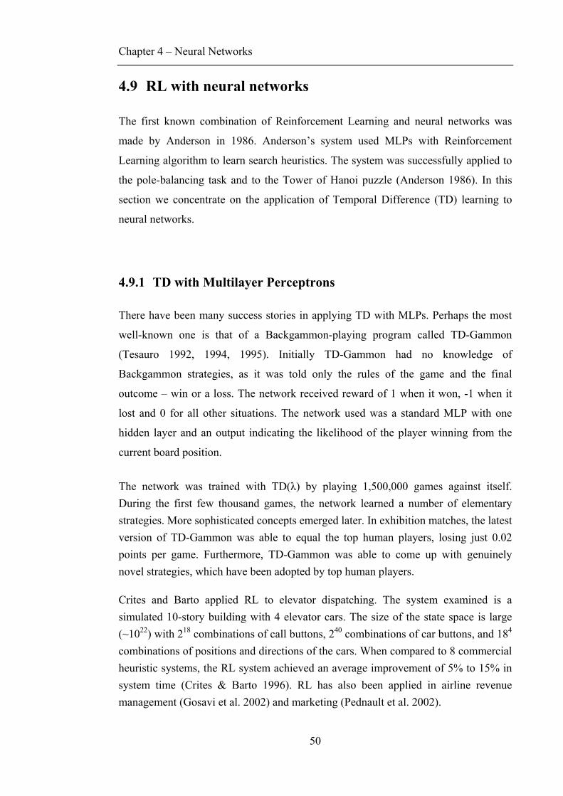
Chapter 4 – Neural Networks
50
4.9 RL with neural networks
The first known combination of Reinforcement Learning and neural networks was
made by Anderson in 1986. Anderson’s system used MLPs with Reinforcement
Learning algorithm to learn search heuristics. The system was successfully applied to
the pole-balancing task and to the Tower of Hanoi puzzle (Anderson 1986). In this
section we concentrate on the application of Temporal Difference (TD) learning to
neural networks.
4.9.1 TD with Multilayer Perceptrons
There have been many success stories in applying TD with MLPs. Perhaps the most
well-known one is that of a Backgammon-playing program called TD-Gammon
(Tesauro 1992, 1994, 1995). Initially TD-Gammon had no knowledge of
Backgammon strategies, as it was told only the rules of the game and the final
outcome – win or a loss. The network received reward of 1 when it won, -1 when it
lost and 0 for all other situations. The network used was a standard MLP with one
hidden layer and an output indicating the likelihood of the player winning from the
current board position.
The network was trained with TD(λ) by playing 1,500,000 games against itself. During the first few thousand games, the network learned a number of elementary strategies. More sophisticated concepts emerged later. In exhibition matches, the latest version of TD-Gammon was able to equal the top human players, losing just 0.02 points per game. Furthermore, TD-Gammon was able to come up with genuinely novel strategies, which have been adopted by top human players.
Crites and Barto applied RL to elevator dispatching. The system examined is a simulated 10-story building with 4 elevator cars. The size of the state space is large (~1022) with 218 combinations of call buttons, 240 combinations of car buttons, and 184 combinations of positions and directions of the cars. When compared to 8 commercial heuristic systems, the RL system achieved an average improvement of 5% to 15% in system time (Crites & Barto 1996). RL has also been applied in airline revenue management (Gosavi et al. 2002) and marketing (Pednault et al. 2002).
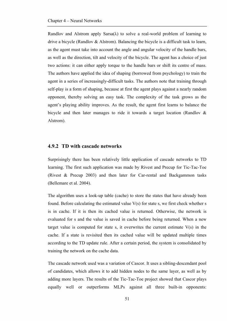
Chapter 4 – Neural Networks
51
Randlov and Alstrom apply Sarsa(λ) to solve a real-world problem of learning to
drive a bicycle (Randlov & Alstrom). Balancing the bicycle is a difficult task to learn,
as the agent must take into account the angle and angular velocity of the handle bars,
as well as the direction, tilt and velocity of the bicycle. The agent has a choice of just
two actions: it can either apply torque to the handle bars or shift its centre of mass.
The authors have applied the idea of shaping (borrowed from psychology) to train the
agent in a series of increasingly-difficult tasks. The authors note that training through
self-play is a form of shaping, because at first the agent plays against a nearly random
opponent, thereby solving an easy task. The complexity of the task grows as the
agent’s playing ability improves. As the result, the agent first learns to balance the
bicycle and then later manages to ride it towards a target location (Randlov &
Alstrom).
4.9.2 TD with cascade networks
Surprisingly there has been relatively little application of cascade networks to TD
learning. The first such application was made by Rivest and Precup for Tic-Tac-Toe
(Rivest & Precup 2003) and then later for Car-rental and Backgammon tasks
(Bellemare et al. 2004).
The algorithm uses a look-up table (cache) to store the states that have already been
found. Before calculating the estimated value V(s) for state s, we first check whether s
is in cache. If it is then its cached value is returned. Otherwise, the network is
evaluated for s and the value is saved in cache before being returned. When a new
target value is computed for state s, it overwrites the current estimate V(s) in the
cache. If a state is revisited then its cached value will be updated multiple times
according to the TD update rule. After a certain period, the system is consolidated by
training the network on the cache data.
The cascade network used was a variation of Cascor. It uses a sibling-descendant pool
of candidates, which allows it to add hidden nodes to the same layer, as well as by
adding more layers. The results of the Tic-Tac-Toe project showed that Cascor plays
equally well or outperforms MLPs against all three built-in opponents:
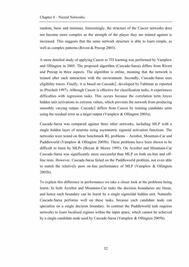
Chapter 4 – Neural Networks
52
random, basic and minimax. Interestingly, the structure of the Cascor networks does
not become more complex as the strength of the player they are trained against is
increased. This suggests that the same network structure is able to learn simple, as
well as complex patterns (Rivest & Precup 2003).
A more detailed study of applying Cascor to TD learning was performed by Vamplew and Ollington in 2005. The proposed algorithm (Cascade-Sarsa) differs from Rivest and Precup in three aspects. The algorithm is online, meaning that the network is trained after each interaction with the environment. Secondly, Cascade-Sarsa uses eligibility traces. Finally, it is based on Cascade2, developed by Fahlman as reported in (Prechelt 1997). Although Cascor is effective for classification tasks, it experiences difficulties with regression tasks. This occurs because the correlation term forces hidden unit activations to extreme values, which prevents the network from producing smoothly varying output. Cascade2 differs from Cascor by training candidate units using the residual error as a target output (Vamplew & Ollington 2005a).
Cascade-Sarsa was compared against three other networks, including MLP with a single hidden layer of neurons using asymmetric sigmoid activation functions. The networks were tested on three benchmark RL problems – Acrobot, Mountain-Car and Puddleworld (Vamplew & Ollington 2005b). These problems have been shown to be difficult to learn by MLPs (Boyan & Moore 1995). On Acrobot and Mountain-Car Cascade-Sarsa was significantly more successful than MLP on both on-line and off-line tests. However, Cascade-Sarsa failed on the Puddleworld problem, not even able to match the relatively poor on-line performance of MLP (Vamplew & Ollington 2005b).
To explain this difference in performance we take a closer look at the problems being learnt. In both Acrobot and Mountain-Car tasks the decision boundaries are linear, and hence each boundary can be learnt by a single sigmoidal hidden unit. Naturally Cascade-Sarsa performs well on these tasks, because each candidate node can specialize on a single decision boundary. In contrast the Puddleworld task requires networks to learn localised regions within the input space, which cannot be achieved by a single candidate node used by Cascade-Sarsa (Vamplew & Ollington 2005b).

Chapter 5 – Othello
53
Chapter 5 Othello
5.1 History of the game
Formally speaking, Othello is a two-person zero-sum deterministic finite board game
with perfect information. Two-person zero-sum games are characterized by the fact
that either one player wins and the other loses, or neither player wins (tie). It is not
possible for both players to win. Deterministic games are games where there are no
random events such as the roll of a dice. Othello is a finite game, because there is a
finite number of moves: at most 60. Othello has perfect information, because all the
game information such as piece position is available to all players.
The exact origins of Othello are not known, although it is believed to have originated
from the Chinese game ‘Fan Mian’, which translates to ‘reverse’ (hence the
alternative name Reversi). Until recently the game has been primarily played in Japan,
where it is the second most popular game next to Go.
In 1890’s a game called Reversi was being marketed in England by Jaques and Sons
of London. This game was very similar to the modern game except for two
differences:
1. Each player was given a set number of discs at the start of the game. If a
player ran out of discs, his opponent completed the remainder of the game.
2. The game began with an empty board.
In 1975 Goro Hasegawa introduced the modern version of Othello which has been
adopted across the world. In the modern version, players take from a central pool of
discs and the initial layout of four discs is provided. Othello is fast growing in
popularity with major international tournaments held every year. It has also been a
popular test-bed for AI research (Buro 1994; Lee & Mahajan 1990; Rosenbloom
1982).
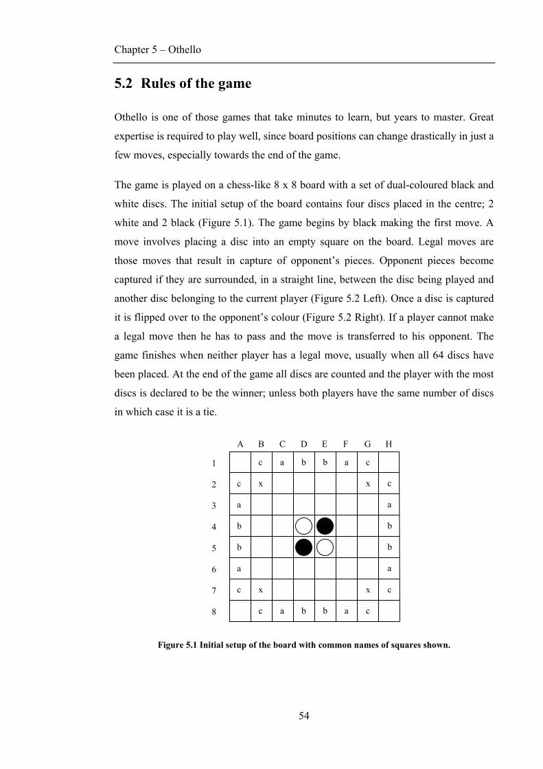
Chapter 5 – Othello
54
5.2 Rules of the game
Othello is one of those games that take minutes to learn, but years to master. Great
expertise is required to play well, since board positions can change drastically in just a
few moves, especially towards the end of the game.
The game is played on a chess-like 8 x 8 board with a set of dual-coloured black and
white discs. The initial setup of the board contains four discs placed in the centre; 2
white and 2 black (Figure 5.1). The game begins by black making the first move. A
move involves placing a disc into an empty square on the board. Legal moves are
those moves that result in capture of opponent’s pieces. Opponent pieces become
captured if they are surrounded, in a straight line, between the disc being played and
another disc belonging to the current player (Figure 5.2 Left). Once a disc is captured
it is flipped over to the opponent’s colour (Figure 5.2 Right). If a player cannot make
a legal move then he has to pass and the move is transferred to his opponent. The
game finishes when neither player has a legal move, usually when all 64 discs have
been placed. At the end of the game all discs are counted and the player with the most
discs is declared to be the winner; unless both players have the same number of discs
in which case it is a tie.
Figure 5.1 Initial setup of the board with common names of squares shown.
1
2
3
4
5
6
7
8
A B C D E F G H
a a b b c c
a a b b c c
c
a
b
b
a
c
c
a
b
b
a
c
x x
x x
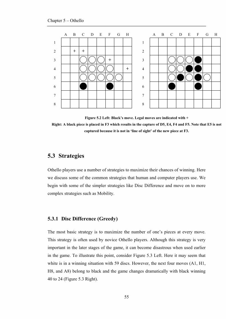
Chapter 5 – Othello
55
Figure 5.2 Left: Black’s move. Legal moves are indicated with +
Right: A black piece is placed in F3 which results in the capture of D5, E4, F4 and F5. Note that E5 is not
captured because it is not in ‘line of sight’ of the new piece at F3.
5.3 Strategies
Othello players use a number of strategies to maximize their chances of winning. Here
we discuss some of the common strategies that human and computer players use. We
begin with some of the simpler strategies like Disc Difference and move on to more
complex strategies such as Mobility.
5.3.1 Disc Difference (Greedy)
The most basic strategy is to maximize the number of one’s pieces at every move.
This strategy is often used by novice Othello players. Although this strategy is very
important in the later stages of the game, it can become disastrous when used earlier
in the game. To illustrate this point, consider Figure 5.3 Left. Here it may seem that
white is in a winning situation with 59 discs. However, the next four moves (A1, H1,
H8, and A8) belong to black and the game changes dramatically with black winning
40 to 24 (Figure 5.3 Right).
1
2
3
4
5
6
7
8
A B C D E F G H H
1
2
3
4
5
6
7
8
A B C D E F G
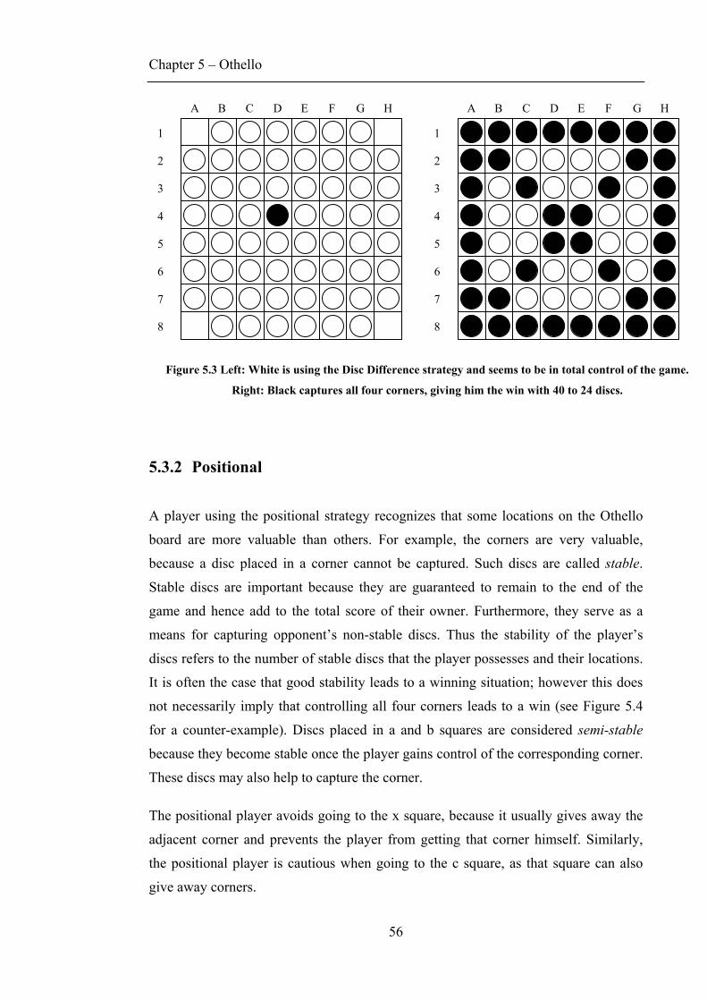
Chapter 5 – Othello
56
Figure 5.3 Left: White is using the Disc Difference strategy and seems to be in total control of the game.
Right: Black captures all four corners, giving him the win with 40 to 24 discs.
5.3.2 Positional
A player using the positional strategy recognizes that some locations on the Othello
board are more valuable than others. For example, the corners are very valuable,
because a disc placed in a corner cannot be captured. Such discs are called stable.
Stable discs are important because they are guaranteed to remain to the end of the
game and hence add to the total score of their owner. Furthermore, they serve as a
means for capturing opponent’s non-stable discs. Thus the stability of the player’s
discs refers to the number of stable discs that the player possesses and their locations.
It is often the case that good stability leads to a winning situation; however this does
not necessarily imply that controlling all four corners leads to a win (see Figure 5.4
for a counter-example). Discs placed in a and b squares are considered semi-stable
because they become stable once the player gains control of the corresponding corner.
These discs may also help to capture the corner.
The positional player avoids going to the x square, because it usually gives away the
adjacent corner and prevents the player from getting that corner himself. Similarly,
the positional player is cautious when going to the c square, as that square can also
give away corners.
1
2
3
4
5
6
7
8
A B C D E F G H
1
2
3
4
5
6
7
8
A B C D E F G H
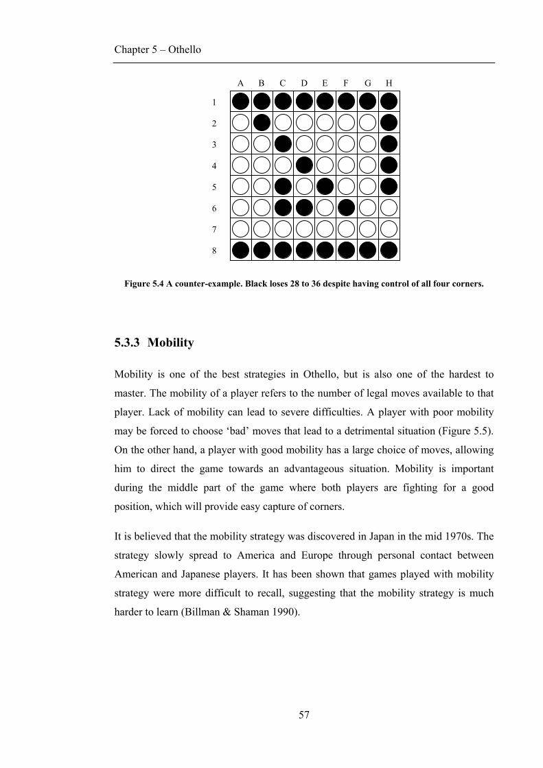
Chapter 5 – Othello
57
Figure 5.4 A counter-example. Black loses 28 to 36 despite having control of all four corners.
5.3.3 Mobility
Mobility is one of the best strategies in Othello, but is also one of the hardest to
master. The mobility of a player refers to the number of legal moves available to that
player. Lack of mobility can lead to severe difficulties. A player with poor mobility
may be forced to choose ‘bad’ moves that lead to a detrimental situation (Figure 5.5).
On the other hand, a player with good mobility has a large choice of moves, allowing
him to direct the game towards an advantageous situation. Mobility is important
during the middle part of the game where both players are fighting for a good
position, which will provide easy capture of corners.
It is believed that the mobility strategy was discovered in Japan in the mid 1970s. The
strategy slowly spread to America and Europe through personal contact between
American and Japanese players. It has been shown that games played with mobility
strategy were more difficult to recall, suggesting that the mobility strategy is much
harder to learn (Billman & Shaman 1990).
1
2
3
4
5
6
7
8
A B C D E F G H
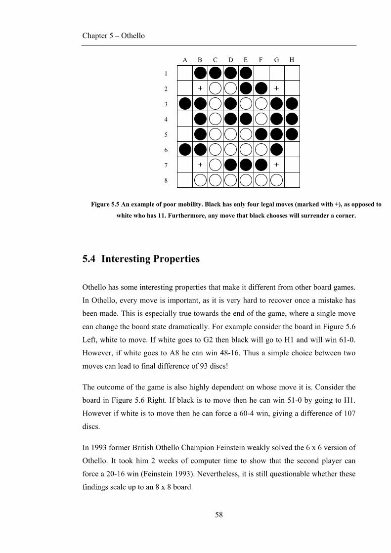
Chapter 5 – Othello
58
Figure 5.5 An example of poor mobility. Black has only four legal moves (marked with +), as opposed to
white who has 11. Furthermore, any move that black chooses will surrender a corner.
5.4 Interesting Properties
Othello has some interesting properties that make it different from other board games.
In Othello, every move is important, as it is very hard to recover once a mistake has
been made. This is especially true towards the end of the game, where a single move
can change the board state dramatically. For example consider the board in Figure 5.6
Left, white to move. If white goes to G2 then black will go to H1 and will win 61-0.
However, if white goes to A8 he can win 48-16. Thus a simple choice between two
moves can lead to final difference of 93 discs!
The outcome of the game is also highly dependent on whose move it is. Consider the
board in Figure 5.6 Right. If black is to move then he can win 51-0 by going to H1.
However if white is to move then he can force a 60-4 win, giving a difference of 107
discs.
In 1993 former British Othello Champion Feinstein weakly solved the 6 x 6 version of
Othello. It took him 2 weeks of computer time to show that the second player can
force a 20-16 win (Feinstein 1993). Nevertheless, it is still questionable whether these
findings scale up to an 8 x 8 board.
1
2
3
4
5
6
7
8
A B C D E F G H
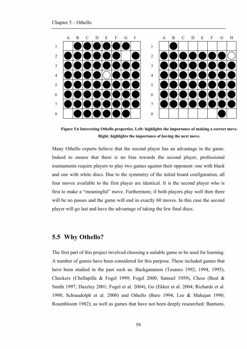
Chapter 5 – Othello
59
Figure 5.6 Interesting Othello properties. Left: highlights the importance of making a correct move.
Right: highlights the importance of having the next move.
Many Othello experts believe that the second player has an advantage in the game.
Indeed to ensure that there is no bias towards the second player, professional
tournaments require players to play two games against their opponent: one with black
and one with white discs. Due to the symmetry of the initial board configuration, all
four moves available to the first player are identical. It is the second player who is
first to make a “meaningful” move. Furthermore, if both players play well then there
will be no passes and the game will end in exactly 60 moves. In this case the second
player will go last and have the advantage of taking the few final discs.
5.5 Why Othello?
The first part of this project involved choosing a suitable game to be used for learning.
A number of games have been considered for this purpose. These included games that
have been studied in the past such as: Backgammon (Tesauro 1992, 1994, 1995),
Checkers (Chellapilla & Fogel 1999; Fogel 2000; Samuel 1959), Chess (Beal &
Smith 1997; Dazeley 2001; Fogel et al. 2004), Go (Ekker et al. 2004; Richards et al.
1998; Schraudolph et al. 2000) and Othello (Buro 1994; Lee & Mahajan 1990;
Rosenbloom 1982); as well as games that have not been deeply researched: Bantumi,
1
2
3
4
5
6
7
8
A B C D E F G H
1
2
3
4
5
6
7
8
A B C D E F G H
Chapter 5 – Othello
60
Chinese checkers and Lines. Othello was chosen for the following reasons:
• It is a well-studied game, researched by many authors using a variety of
techniques.
• The rules of the game are simple and easy to implement.
• It is easy to implement basic AI opponents, such as a random player and a
greedy player.
• From Table 5.1 in section 5.5.4, we can see that Othello has a reasonable
complexity. It is not as simple as Checkers and not as complex as Chess or
Go.
• Since every game is guaranteed to finish in 60 moves or less, Othello is
perfect for rapid training of neural networks.
Ghory identifies four game properties that are crucial for a successful game playing
agent that is based on TD-Learning: board smoothness, board divergence, forced
exploration, state-space complexity (Ghory 2004).
5.5.1 Board smoothness
It is known that neural networks are better at learning smooth functions. A function
f(x) is smooth if a small change in x implies a small change in f(x). Hence, if |A – B|
is the absolute difference between two board states A and B then we want a small
value in |A – B| to correspond to a small value in |e(A) – e(B)|, where e is the board
evaluation function. Board smoothness can be achieved by carefully selecting the
right board representation. The most natural way to represent an M x N board is to
have MN inputs, where each input stores the contents of a single board square. It is
hard to say whether this representation achieves the optimal board smoothness, but it
is a popular choice when it comes to representing Othello boards (Deshwal & Kasera
2003; Leouski 1995; Tournavitis 2003; Walker et al. 1994).
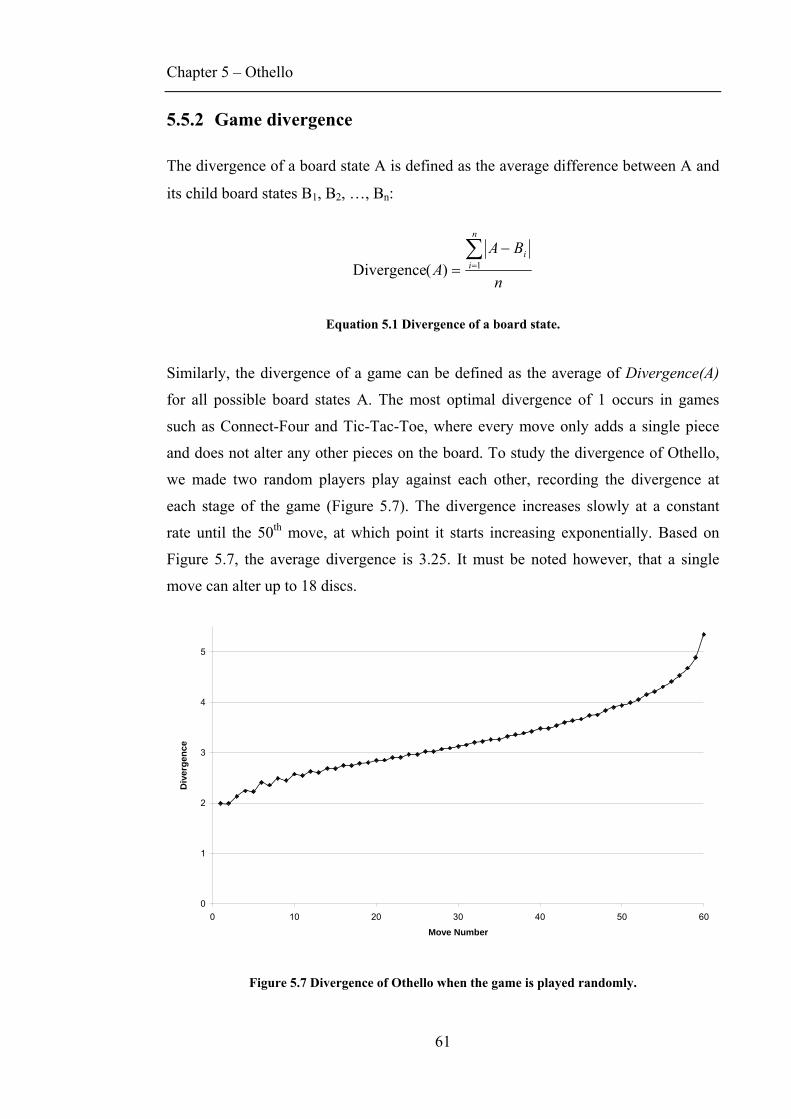
Chapter 5 – Othello
61
5.5.2 Game divergence
The divergence of a board state A is defined as the average difference between A and
its child board states B1, B2, …, Bn:
n
BAA
n
ii∑
=
−= 1)(Divergence
Equation 5.1 Divergence of a board state.
Similarly, the divergence of a game can be defined as the average of Divergence(A)
for all possible board states A. The most optimal divergence of 1 occurs in games
such as Connect-Four and Tic-Tac-Toe, where every move only adds a single piece
and does not alter any other pieces on the board. To study the divergence of Othello,
we made two random players play against each other, recording the divergence at
each stage of the game (Figure 5.7). The divergence increases slowly at a constant
rate until the 50th move, at which point it starts increasing exponentially. Based on
Figure 5.7, the average divergence is 3.25. It must be noted however, that a single
move can alter up to 18 discs.
0
1
2
3
4
5
0 10 20 30 40 50 60
Move Number
Div
erge
nce
Figure 5.7 Divergence of Othello when the game is played randomly.
Chapter 5 – Othello
62
5.5.3 Forced exploration
There is a general consensus amongst AI researchers that a learning agent should not
always choose the best move available as this will restrict his knowledge of the
environment. Occasionally, the agent should choose a weaker move in order to
explore new possibilities and hopefully learn a better strategy. Games that have a
random element such as Backgammon or Poker are ideal, because they force the agent
to explore. Pollack and Blair claim that forced exploration of Backgammon was one
of the main reasons for the success of Tesauro’s TD-Gammon (Pollack & Blair).
However, it is still possible to force exploration in deterministic games by introducing
randomness to the move selection strategy.
5.5.4 State-space complexity
State-space complexity is defined as the number of board states that can occur in a
game. It is important to know the state-space complexity as it defines the domain of
the board evaluation function. Thus the larger the state-space complexity the longer it
will take to train the board evaluation function. Van Den Herik et al. (2002) present
state-space and game tree complexities of some games (Table 5.1). If we assume that
any of Othello’s 64 board locations can take three values (black, empty, white) then
we can calculate the upper boundary for Othello’s state-space complexity to be 364 ≈
3.4 x 1030. This value indicates that less than 0.3% of theoretical board states are
possible during the actual game. Ghory estimates that it is possible to produce a
strong TD-Learning based agent for any game whose state-space complexity is less
than 1020. He goes on to claim that the state-space complexity of a game is the single
most important factor out of the four game properties discussed (Ghory 2004).
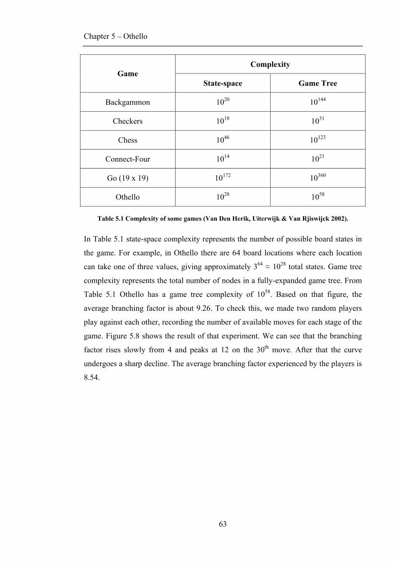
Chapter 5 – Othello
63
Complexity Game
State-space Game Tree
Backgammon 1020 10144
Checkers 1018 1031
Chess 1046 10123
Connect-Four 1014 1021
Go (19 x 19) 10172 10360
Othello 1028 1058
Table 5.1 Complexity of some games (Van Den Herik, Uiterwijk & Van Rjiswijck 2002).
In Table 5.1 state-space complexity represents the number of possible board states in
the game. For example, in Othello there are 64 board locations where each location
can take one of three values, giving approximately 364 ≈ 1028 total states. Game tree
complexity represents the total number of nodes in a fully-expanded game tree. From
Table 5.1 Othello has a game tree complexity of 1058. Based on that figure, the
average branching factor is about 9.26. To check this, we made two random players
play against each other, recording the number of available moves for each stage of the
game. Figure 5.8 shows the result of that experiment. We can see that the branching
factor rises slowly from 4 and peaks at 12 on the 30th move. After that the curve
undergoes a sharp decline. The average branching factor experienced by the players is
8.54.
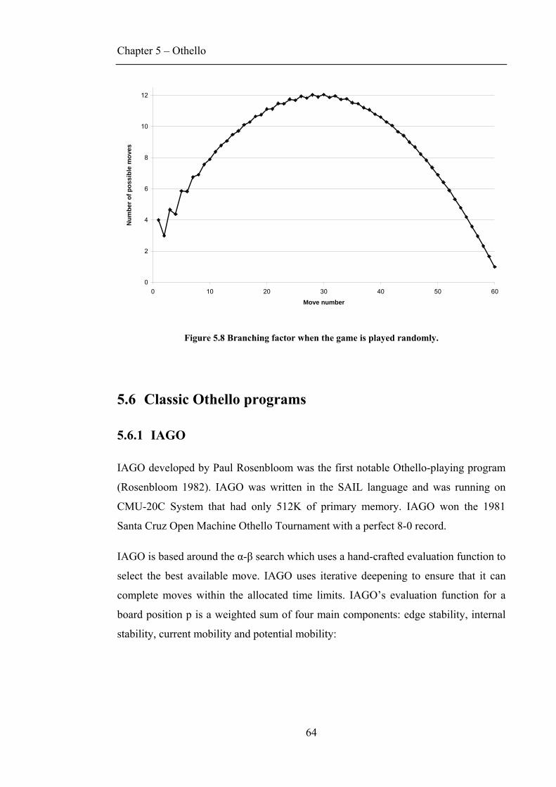
Chapter 5 – Othello
64
0
2
4
6
8
10
12
0 10 20 30 40 50 60
Move number
Num
ber o
f pos
sibl
e m
oves
Figure 5.8 Branching factor when the game is played randomly.
5.6 Classic Othello programs
5.6.1 IAGO
IAGO developed by Paul Rosenbloom was the first notable Othello-playing program
(Rosenbloom 1982). IAGO was written in the SAIL language and was running on
CMU-20C System that had only 512K of primary memory. IAGO won the 1981
Santa Cruz Open Machine Othello Tournament with a perfect 8-0 record.
IAGO is based around the α-β search which uses a hand-crafted evaluation function to
select the best available move. IAGO uses iterative deepening to ensure that it can
complete moves within the allocated time limits. IAGO’s evaluation function for a
board position p is a weighted sum of four main components: edge stability, internal
stability, current mobility and potential mobility:
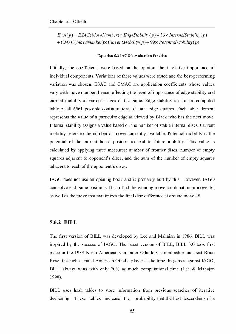
Chapter 5 – Othello
65
)(99)()()(36)()()(
pobilityPotentialMpilityCurrentMobMoveNumberCMACpabilityInternalStpityEdgeStabilMoveNumberESACpEval
×+×+×+×=
Equation 5.2 IAGO's evaluation function
Initially, the coefficients were based on the opinion about relative importance of
individual components. Variations of these values were tested and the best-performing
variation was chosen. ESAC and CMAC are application coefficients whose values
vary with move number, hence reflecting the level of importance of edge stability and
current mobility at various stages of the game. Edge stability uses a pre-computed
table of all 6561 possible configurations of eight edge squares. Each table element
represents the value of a particular edge as viewed by Black who has the next move.
Internal stability assigns a value based on the number of stable internal discs. Current
mobility refers to the number of moves currently available. Potential mobility is the
potential of the current board position to lead to future mobility. This value is
calculated by applying three measures: number of frontier discs, number of empty
squares adjacent to opponent’s discs, and the sum of the number of empty squares
adjacent to each of the opponent’s discs.
IAGO does not use an opening book and is probably hurt by this. However, IAGO
can solve end-game positions. It can find the winning move combination at move 46,
as well as the move that maximizes the final disc difference at around move 48.
5.6.2 BILL
The first version of BILL was developed by Lee and Mahajan in 1986. BILL was
inspired by the success of IAGO. The latest version of BILL, BILL 3.0 took first
place in the 1989 North American Computer Othello Championship and beat Brian
Rose, the highest rated American Othello player at the time. In games against IAGO,
BILL always wins with only 20% as much computational time (Lee & Mahajan
1990).
BILL uses hash tables to store information from previous searches of iterative
deepening. These tables increase the probability that the best descendants of a
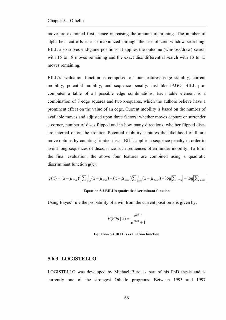
Chapter 5 – Othello
66
move are examined first, hence increasing the amount of pruning. The number of
alpha-beta cut-offs is also maximized through the use of zero-window searching.
BILL also solves end-game positions. It applies the outcome (win/loss/draw) search
with 15 to 18 moves remaining and the exact disc differential search with 13 to 15
moves remaining.
BILL’s evaluation function is composed of four features: edge stability, current
mobility, potential mobility, and sequence penalty. Just like IAGO, BILL pre-
computes a table of all possible edge combinations. Each table element is a
combination of 8 edge squares and two x-squares, which the authors believe have a
prominent effect on the value of an edge. Current mobility is based on the number of
available moves and adjusted upon three factors: whether moves capture or surrender
a corner, number of discs flipped and in how many directions, whether flipped discs
are internal or on the frontier. Potential mobility captures the likelihood of future
move options by counting frontier discs. BILL applies a sequence penalty in order to
avoid long sequences of discs, since such sequences often hinder mobility. To form
the final evaluation, the above four features are combined using a quadratic
discriminant function g(x):
∑∑∑∑ −+−−−−−=−−
LossWinLoss LossLossWin WinT
Win xxxxxg loglog)()()()()( 11 μμμμ
Equation 5.3 BILL's quadratic discriminant function
Using Bayes’ rule the probability of a win from the current position x is given by:
1)|( )(
)(
+= xg
xg
eexWinP
Equation 5.4 BILL's evaluation function
5.6.3 LOGISTELLO
LOGISTELLO was developed by Michael Buro as part of his PhD thesis and is
currently one of the strongest Othello programs. Between 1993 and 1997
Chapter 5 – Othello
67
LOGISTELLO dominated all computer Othello tournaments by winning 18 out of a
total of 25. In 1997 LOGISTELLO defeated the reigning World Champion Takeshi
Murakami by winning 6-0.
Although BILL showed a strong performance, many of its features still relied on
manually-tuned parameters. The main idea behind LOGISTELLO is to learn pattern
values from sample data – rather than guessing them (Buro 2003). LOGISTELLO
treats the game as 13 separate stages: 13-16 discs, 17-20 discs, … , 61-64 discs (for
fewer than 13 discs the opening book is used). Each game stage has a different set of
weights in the evaluation function. The evaluation function analyses 46 patterns of
squares that capture important strategic concepts such as mobility, stability and parity.
These patterns include all diagonals longer than 3 squares, all rows, as well as 2x5
and 3x3 corner regions. The evaluation of a particular board approximates the final
disc differential by summing up the weights associated with the matching patterns.
Buro made a considerable effort to develop LOGISTELLO’s opening book. The
opening book is a table of precomputed evaluations for most common game openings.
LOGISTELLO has learnt its opening book from 23000 tournament games and
evaluations of “best” move alternatives. Furthermore, it continues to learn with every
new game and thus is guaranteed not to make the same mistake twice.
To speed up the searching procedure Buro introduced a method called ProbCut.
ProbCut prunes sub-trees that are unlikely to yield a good solution. The time saved is
used to explore better possibilities (Buro 1995). An extension to ProbCut is Multi-
ProbCut, which can prune at different search depths, uses game-stage dependent cut
thresholds, and performs shallow check searches (Buro 2003). The combination of
these improvements allow LOGISTELLO to perform an outcome end-game search
with 22-26 moves remaining and an exact search with 20-24 moves remaining.
5.7 Othello programs using TD
There have been a number of applications of TD to Othello (Cranney 2002; Deshwal
& Kasera 2003; Leouski 1995; Tournavitis 2003; van Eck & van Wezel 2004; Walker
Chapter 5 – Othello
68
et al. 1994). In this section we discuss three applications that are most relevant to this
project.
The earliest application of TD to Othello was in 1994 (Walker et al. 1994). The aim of
that research was to replicate the results of Tesauro in Othello to form TD-Othello.
Unlike Backgammon, Othello is deterministic and noise needs to be added. The
authors simulate noise by adding a random value εm to the output of the network, with
εm uniformly distributed in the range [-0.1, 0.1]. In essence this is similar to softmax
selection: the moves that were ranked highly before noise was added are also likely to
rank highly with noise and hence will be selected; moves that ranked lowly will
remain ranked lowly and hence will not be selected. As the result of just 30,000 self-
play games the agent was able to win against the Novice (2nd) level player of
Windows Reversi (Version 2.03). Furthermore, by providing a one-step look ahead
the agent managed to consistently beat Windows Reversi at the Expert (3rd) level, and
even had occasional wins at the Master (4th) level. Due to its ability to beat a
commercial product, TD-Othello was chosen as a base model to develop the Othello
player for this project.
Leouski draws attention to the fact that the Othello board is symmetrical with respect
to reflections and rotations (Leouski 1995). This symmetry is incorporated into the
network by appropriate weight sharing (Rumelhart et al. 1986) and summing of
derivatives. The initial network was able to win 42% against Wystan (Clouse 1992), a
program that incorporates several high-level features such as mobility and stability.
Leouski then creates an agent that uses three separate networks – one for each stage of
the game. This improves the agent’s performance considerably as it is able to win
73% against Wystan. The author postulates that the agent’s performance can be
boosted further by growing the network dynamically as it learns. This is exactly what
our project aims to test.
Cranney makes comparisons between self-play and tournament-play learning applied
to Othello (Cranney 2002). In tournament-play, multiple agents are trained by playing
against each other. The author argues that tournament-play leads to greater
exploration, since the networks get to experience a wider range of strategies.
However, this also means that tournament-play is less likely to converge to a good

Chapter 5 – Othello
69
strategy. In conclusion, Cranney shows that self-play outperforms tournament-play
for simple input, but when advanced input encoding is introduced, tournament-play
gains an evident advantage. In this project we are mainly concerned with the agent’s
ability to learn from simple inputs and hence self-play was chosen as the training
method.
Chapter 6 – Method
70
Chapter 6 Method
6.1 Training environment
The program used in this project can be divided into two main environments: training
and testing. In training, the following were taken into account: various input schemes,
action selection strategies, reward function, parameters common to all neural
networks, those specific to the fixed architecture and those specific to the constructive
architecture. In testing, consideration was given to the following: built-in opponents,
ways of measuring learning and other potentially useful features.
6.1.1 Input representation
In Reinforcement Learning problems the success of the learning agent is highly
dependent upon the input representation used. It is important to remember that we are
teaching a computer agent to learn, not a human agent. Inputs that can be easily
interpreted by a human, such as a picture of a fish, are not necessarily easy to interpret
for a computer. Indeed this is one of the main reasons why computer vision is still in
its infancy. On the other hand, inputs that are long strings of ‘0’ and ‘1’ are difficult
for humans to interpret, but can be easily used by a computer. After all, computers are
designed to manipulate large amounts of information represented as strings of ‘0’ and
‘1’.
The input we provide must describe the environment without oversimplifying or
overcomplicating it. If the input is oversimplified then we risk losing some
information about the environment and hence our network will receive an incomplete
picture. If the input is overcomplicated then the network will struggle to make
generalizations from it and as a result will not learn.
The purpose of this project is not to develop a system that plays exceptionally well in
Othello. Instead, we want to develop a system that is able to learn good
Chapter 6 – Method
71
strategies starting from scratch, just like a novice human would. Therefore in order to
test the agent’s learning abilities, we try to avoid providing additional information
such as: disc count, mobility and stability.
6.1.1.1 Simple
The simple input representation, as the name suggests, is the simplest way of
representing the Othello board without losing any information. The contents of each
board square are represented by a single input. Since a white disc is an exact opposite
to a black disc it makes sense for them to have opposing input values. Continuing
with this logic the value of an empty square must be between that of white and black
to avoid any bias. Thus the inputs used were 0.0, 0.5 and 1.0 for white, empty and
black respectively. The last input in the representation indicates whose move it is,
which is a crucial piece of information for the learning agent. This input is set to 1 if it
is black’s move and 0 for white’s move.
6.1.1.2 Simple2
Unlike the Simple representation, Simple2 uses two inputs for each square. The first
input is on if the square contains black, while the second input is on if the square
contains white. If both inputs are off then the square is empty (note that both inputs
are never on). This representation has both advantages and disadvantages over the
Simple representation. Firstly it ensures that all inputs are binary, which is perhaps
easier for the network to learn. On the other hand, the amount of information needed
to be learned is doubled, which may reduce the convergence rate.
6.1.1.3 Walker
This representation was used by one of the first applications of TD to Othello, and
hence was also the one tried for this project (Walker et al. 1994). The input consists of
129 units: two sets of 64 units each and an extra unit indicating the player about
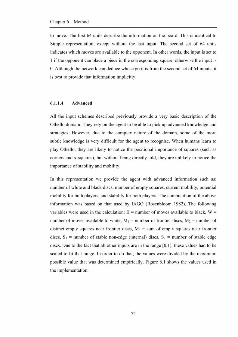
Chapter 6 – Method
72
to move. The first 64 units describe the information on the board. This is identical to
Simple representation, except without the last input. The second set of 64 units
indicates which moves are available to the opponent. In other words, the input is set to
1 if the opponent can place a piece in the corresponding square, otherwise the input is
0. Although the network can deduce whose go it is from the second set of 64 inputs, it
is best to provide that information implicitly.
6.1.1.4 Advanced
All the input schemes described previously provide a very basic description of the
Othello domain. They rely on the agent to be able to pick up advanced knowledge and
strategies. However, due to the complex nature of the domain, some of the more
subtle knowledge is very difficult for the agent to recognise. When humans learn to
play Othello, they are likely to notice the positional importance of squares (such as
corners and x-squares), but without being directly told, they are unlikely to notice the
importance of stability and mobility.
In this representation we provide the agent with advanced information such as:
number of white and black discs, number of empty squares, current mobility, potential
mobility for both players, and stability for both players. The computation of the above
information was based on that used by IAGO (Rosenbloom 1982). The following
variables were used in the calculation: B = number of moves available to black, W =
number of moves available to white, M1 = number of frontier discs, M2 = number of
distinct empty squares near frontier discs, M3 = sum of empty squares near frontier
discs, S1 = number of stable non-edge (internal) discs, S2 = number of stable edge
discs. Due to the fact that all other inputs are in the range [0,1], these values had to be
scaled to fit that range. In order to do that, the values were divided by the maximum
possible value that was determined empirically. Figure 6.1 shows the values used in
the implementation.
Chapter 6 – Method
73
⎭⎬⎫
⎩⎨⎧=
⎭⎬⎫
⎩⎨⎧=
+++
=
28,
36
84,
37,
27
21
21
321
SSStability
MMMobilityPotentialM
WBBilityCurrentMob
Figure 6.1 Values used by the Advanced input representation.
It must be noted that this input scheme was developed solely for the purpose of
creating a better Othello player, and not for testing the learning algorithms. The extra
inputs were not directly learned by the agent and were encoded manually.
6.1.1.5 Partial
In all previous representations the inputs were given as a stream with no distinction
made between different rows or columns. The problem with this is that the network
does not know the spatial relationships between each square. In other words, it has no
idea that the inputs represent a two-dimensional board, as far as it is concerned, the
squares are located completely randomly. There must be a way to tell the network that
square A1 is adjacent to A2, which in turn is adjacent to A3. Most importantly for
Othello, the networks must know that corner squares are adjacent to x-squares.
One method of doing this is to create a partially connected neural network, which has
a hidden node for each row, column and diagonal of length 3 or more, so 38 in total.
The idea behind this is to provide the network with all combinations of squares that
can experience flipping (flips in Othello occur only on straight lines). Figure 6.2
demonstrates this idea for a simple 3 x 3 board.

Chapter 6 – Method
74
Figure 6.2 An example of a partially connected network for a 3x3 board. For clarity, only
connections to Row 1, Column 1 and Diagonal 1 are highlighted.
6.1.2 Action Selection
In this study we train a single network for both players. This means that action
selection varies based on whose move it is. The way our reward system is set up, the
black player maximizes the reward, while the white player minimizes it. Similarly, the
black player must select actions that produce a high output, while the white player
selects actions that produce a low output. We have considered 3 strategies for action
selection: ε-greedy, softrank and softmax.
6.1.2.1 ε-greedy
ε-greedy action selection was the first selection algorithm used, because it is by far the
a b c
d e f
g h i
a
b
c
d
e
f
g
h
i
Row 1
Row 2
Row 3
Column 1
Column 2
Column 3
Diagonal 1
Diagonal 2
output
Row 1
Row 2
Row 3
Col
umn
1
Col
umn
2
Col
umn
3
Diagonal 2
Diagonal 1
Chapter 6 – Method
75
easiest to implement. As you recall from section 3.7.1, ε-greedy selects a random
action with probability ε and otherwise selects the best available action. The choice of
ε was based on the value used by (Vamplew & Ollington 2005a). In the initial
experiments ε was set to a constant value of 0.2. Benda suggested that after a period
of 15,000 games, exploration should be reduced by changing ε to 0.05 (Benda July
2005, personal communication). All subsequent experiments used this strategy.
Tournavitis proposes a variation to the ε-greedy strategy. The first n moves are played
randomly (4 ≤ n ≤ 8) and the remaining moves are chosen with ε-greedy. This strategy
was not considered, because it requires the tuning of an additional parameter.
6.1.2.2 Softrank
After using the ε-greedy strategy an attempt was made to implement softmax
selection. However, instead of selecting based on the relative values, like in softmax,
selection was based on the relative ranking of the actions. In other words, the best
ranked action has the highest probability of being selected, followed by the second-
best ranked action and so on. This selection method is referred to as softrank. The
probability of selecting the ith-ranked action from n available actions is given by:
⎟⎠
⎞⎜⎝
⎛−−
÷−− ∑
=
n
kki C
CCC
1 11
11
Equation 6.1 Softrank selection.
The constant C used by Equation 6.1 was chosen to be 1.5. For example, if n = 5 then
the probabilities are given as {55.3%, 22.1%, 11.6%, 6.8%, 4.2%}. Note that softrank
was only used as a trial and is not reported in the results section.
6.1.2.3 Softmax
Recall softmax selection described in section 3.7.2. In theory, this type of selection is
better than ε-greedy, because it gives “direction” to the exploration strategy. Softmax
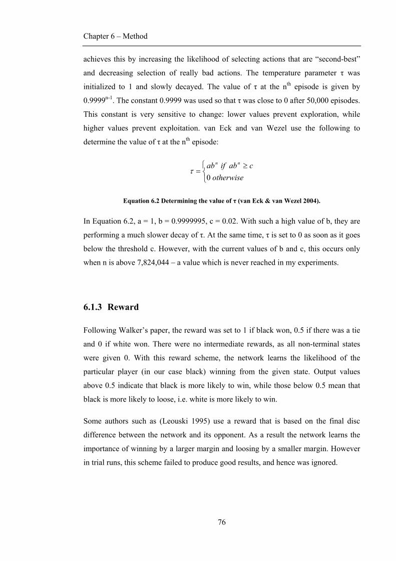
Chapter 6 – Method
76
achieves this by increasing the likelihood of selecting actions that are “second-best”
and decreasing selection of really bad actions. The temperature parameter τ was
initialized to 1 and slowly decayed. The value of τ at the nth episode is given by
0.9999n-1. The constant 0.9999 was used so that τ was close to 0 after 50,000 episodes.
This constant is very sensitive to change: lower values prevent exploration, while
higher values prevent exploitation. van Eck and van Wezel use the following to
determine the value of τ at the nth episode:
⎩⎨⎧ ≥
=otherwise
cabifab nn
0τ
Equation 6.2 Determining the value of τ (van Eck & van Wezel 2004).
In Equation 6.2, a = 1, b = 0.9999995, c = 0.02. With such a high value of b, they are
performing a much slower decay of τ. At the same time, τ is set to 0 as soon as it goes
below the threshold c. However, with the current values of b and c, this occurs only
when n is above 7,824,044 – a value which is never reached in my experiments.
6.1.3 Reward
Following Walker’s paper, the reward was set to 1 if black won, 0.5 if there was a tie
and 0 if white won. There were no intermediate rewards, as all non-terminal states
were given 0. With this reward scheme, the network learns the likelihood of the
particular player (in our case black) winning from the given state. Output values
above 0.5 indicate that black is more likely to win, while those below 0.5 mean that
black is more likely to loose, i.e. white is more likely to win.
Some authors such as (Leouski 1995) use a reward that is based on the final disc
difference between the network and its opponent. As a result the network learns the
importance of winning by a larger margin and loosing by a smaller margin. However
in trial runs, this scheme failed to produce good results, and hence was ignored.
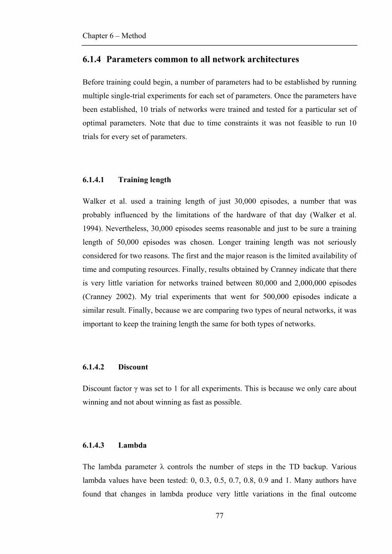
Chapter 6 – Method
77
6.1.4 Parameters common to all network architectures
Before training could begin, a number of parameters had to be established by running
multiple single-trial experiments for each set of parameters. Once the parameters have
been established, 10 trials of networks were trained and tested for a particular set of
optimal parameters. Note that due to time constraints it was not feasible to run 10
trials for every set of parameters.
6.1.4.1 Training length
Walker et al. used a training length of just 30,000 episodes, a number that was
probably influenced by the limitations of the hardware of that day (Walker et al.
1994). Nevertheless, 30,000 episodes seems reasonable and just to be sure a training
length of 50,000 episodes was chosen. Longer training length was not seriously
considered for two reasons. The first and the major reason is the limited availability of
time and computing resources. Finally, results obtained by Cranney indicate that there
is very little variation for networks trained between 80,000 and 2,000,000 episodes
(Cranney 2002). My trial experiments that went for 500,000 episodes indicate a
similar result. Finally, because we are comparing two types of neural networks, it was
important to keep the training length the same for both types of networks.
6.1.4.2 Discount
Discount factor γ was set to 1 for all experiments. This is because we only care about
winning and not about winning as fast as possible.
6.1.4.3 Lambda
The lambda parameter λ controls the number of steps in the TD backup. Various
lambda values have been tested: 0, 0.3, 0.5, 0.7, 0.8, 0.9 and 1. Many authors have
found that changes in lambda produce very little variations in the final outcome
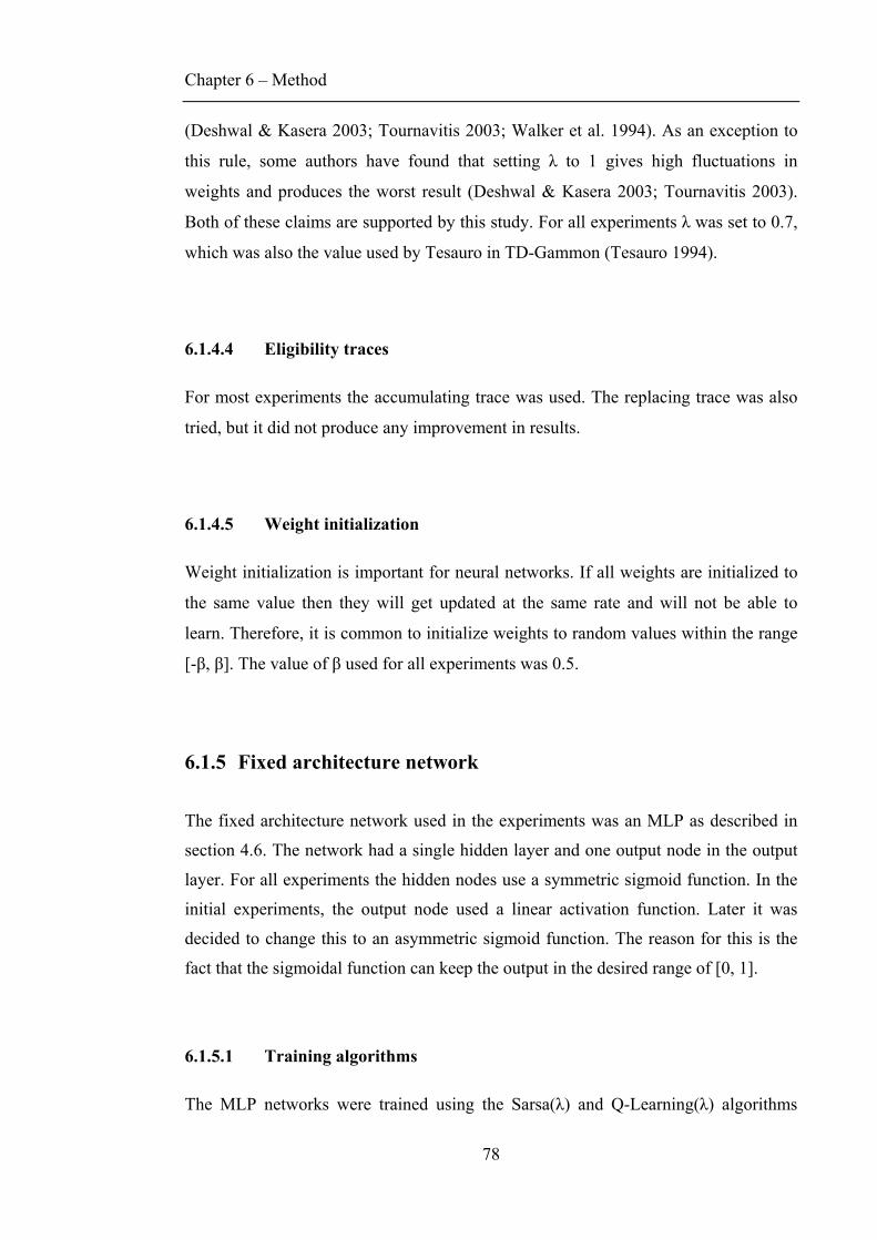
Chapter 6 – Method
78
(Deshwal & Kasera 2003; Tournavitis 2003; Walker et al. 1994). As an exception to
this rule, some authors have found that setting λ to 1 gives high fluctuations in
weights and produces the worst result (Deshwal & Kasera 2003; Tournavitis 2003).
Both of these claims are supported by this study. For all experiments λ was set to 0.7,
which was also the value used by Tesauro in TD-Gammon (Tesauro 1994).
6.1.4.4 Eligibility traces
For most experiments the accumulating trace was used. The replacing trace was also
tried, but it did not produce any improvement in results.
6.1.4.5 Weight initialization
Weight initialization is important for neural networks. If all weights are initialized to
the same value then they will get updated at the same rate and will not be able to
learn. Therefore, it is common to initialize weights to random values within the range
[-β, β]. The value of β used for all experiments was 0.5.
6.1.5 Fixed architecture network
The fixed architecture network used in the experiments was an MLP as described in
section 4.6. The network had a single hidden layer and one output node in the output
layer. For all experiments the hidden nodes use a symmetric sigmoid function. In the
initial experiments, the output node used a linear activation function. Later it was
decided to change this to an asymmetric sigmoid function. The reason for this is the
fact that the sigmoidal function can keep the output in the desired range of [0, 1].
6.1.5.1 Training algorithms
The MLP networks were trained using the Sarsa(λ) and Q-Learning(λ) algorithms
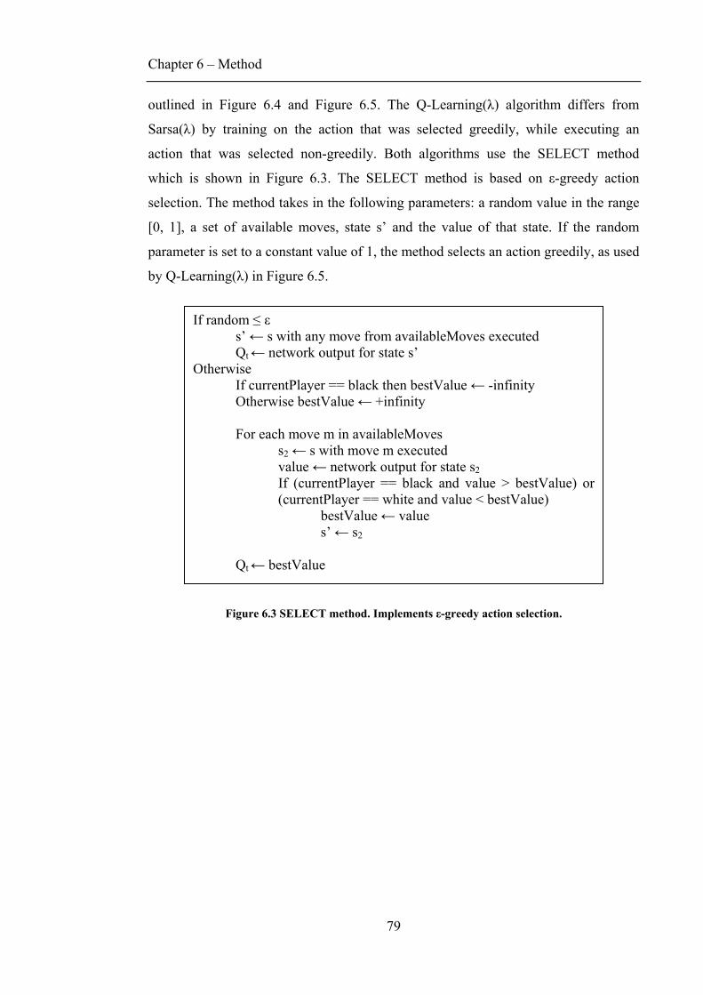
Chapter 6 – Method
79
outlined in Figure 6.4 and Figure 6.5. The Q-Learning(λ) algorithm differs from
Sarsa(λ) by training on the action that was selected greedily, while executing an
action that was selected non-greedily. Both algorithms use the SELECT method
which is shown in Figure 6.3. The SELECT method is based on ε-greedy action
selection. The method takes in the following parameters: a random value in the range
[0, 1], a set of available moves, state s’ and the value of that state. If the random
parameter is set to a constant value of 1, the method selects an action greedily, as used
by Q-Learning(λ) in Figure 6.5.
Figure 6.3 SELECT method. Implements ε-greedy action selection.
If random ≤ ε s’ ← s with any move from availableMoves executed
Qt ← network output for state s’ Otherwise If currentPlayer == black then bestValue ← -infinity Otherwise bestValue ← +infinity For each move m in availableMoves s2 ← s with move m executed value ← network output for state s2
If (currentPlayer == black and value > bestValue) or (currentPlayer == white and value < bestValue) bestValue ← value s’ ← s2
Qt ← bestValue
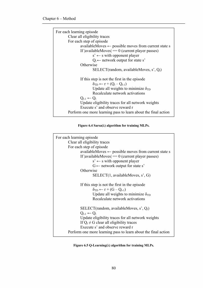
Chapter 6 – Method
80
Figure 6.4 Sarsa(λ) algorithm for training MLPs.
Figure 6.5 Q-Learning(λ) algorithm for training MLPs.
For each learning episode Clear all eligibility traces For each step of episode availableMoves ← possible moves from current state s If |availableMoves| == 0 (current player passes) s’ ← s with opponent player G ← network output for state s’ Otherwise
SELECT(1, availableMoves, s’, G) If this step is not the first in the episode δTD ← r + (G – Qt-1) Update all weights to minimize δTD Recalculate network activations
SELECT(random, availableMoves, s’, Qt) Qt-1 ← Qt Update eligibility traces for all network weights If Qt ≠ G clear all eligibility traces Execute s’ and observe reward r Perform one more learning pass to learn about the final action
For each learning episode Clear all eligibility traces For each step of episode availableMoves ← possible moves from current state s If |availableMoves| == 0 (current player passes) s’ ← s with opponent player Qt ← network output for state s’ Otherwise
SELECT(random, availableMoves, s’, Qt) If this step is not the first in the episode δTD ← r + (Qt – Qt-1) Update all weights to minimize δTD Recalculate network activations Qt-1 ← Qt Update eligibility traces for all network weights Execute s’ and observe reward r Perform one more learning pass to learn about the final action
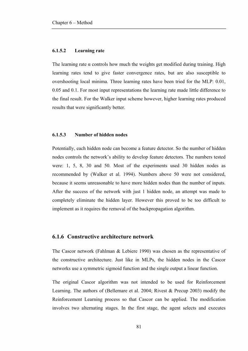
Chapter 6 – Method
81
6.1.5.2 Learning rate
The learning rate α controls how much the weights get modified during training. High
learning rates tend to give faster convergence rates, but are also susceptible to
overshooting local minima. Three learning rates have been tried for the MLP: 0.01,
0.05 and 0.1. For most input representations the learning rate made little difference to
the final result. For the Walker input scheme however, higher learning rates produced
results that were significantly better.
6.1.5.3 Number of hidden nodes
Potentially, each hidden node can become a feature detector. So the number of hidden
nodes controls the network’s ability to develop feature detectors. The numbers tested
were: 1, 5, 8, 30 and 50. Most of the experiments used 30 hidden nodes as
recommended by (Walker et al. 1994). Numbers above 50 were not considered,
because it seems unreasonable to have more hidden nodes than the number of inputs.
After the success of the network with just 1 hidden node, an attempt was made to
completely eliminate the hidden layer. However this proved to be too difficult to
implement as it requires the removal of the backpropagation algorithm.
6.1.6 Constructive architecture network
The Cascor network (Fahlman & Lebiere 1990) was chosen as the representative of
the constructive architecture. Just like in MLPs, the hidden nodes in the Cascor
networks use a symmetric sigmoid function and the single output a linear function.
The original Cascor algorithm was not intended to be used for Reinforcement
Learning. The authors of (Bellemare et al. 2004; Rivest & Precup 2003) modify the
Reinforcement Learning process so that Cascor can be applied. The modification
involves two alternating stages. In the first stage, the agent selects and executes
Chapter 6 – Method
82
actions, and then caches the input state with the target value generated via TD. Once
the cache is full, the network is trained on the cached examples using the Cascor
algorithm. After training, the cache is cleared and the algorithm returns to the first
stage. This new algorithm performs well on Tic-Tac-Toe and car-rental, but does not
do so well on the more complex Backgammon task.
In our experiments we modify the Cascor process so that it can be directly
incorporated into existing Reinforcement Learning algorithms. The new algorithm is
based on Cascade2, developed by Fahlman as reported in (Prechelt 1997). Cascade2
differs from Cascor by training candidates to directly minimise the residual error
rather than to maximise their correlation with that error. This is achieved by training
the output weights, as well as the input weights of each candidate. When the candidate
is added to the network, both its output and input weights are transferred.
6.1.6.1 Weight update algorithm
The original Cascor algorithm uses Quickprop to update the weights (Fahlman 1988).
Quickprop uses an estimate of the second derivative of the error with respect to the
weights to produce faster training of the network. However, Quickprop was designed
for batch-training applications, and hence cannot be used in our situation, where the
weights are updated after every forward pass of the network. For our experiments, the
standard backpropagation algorithm was used instead.
6.1.6.2 Training algorithms
For most experiments, the cascade networks were trained using the modified version
of the Cascade-Sarsa algorithm, which is described in (Vamplew & Ollington 2005a).
This algorithm (Figure 6.6) differs from Cascade-Sarsa, because it is learning state
values and not state-action pairs. For some experiments, the cascade networks were
trained using Q-Learning, which is a combination of Figure 6.5 and Figure 6.6.
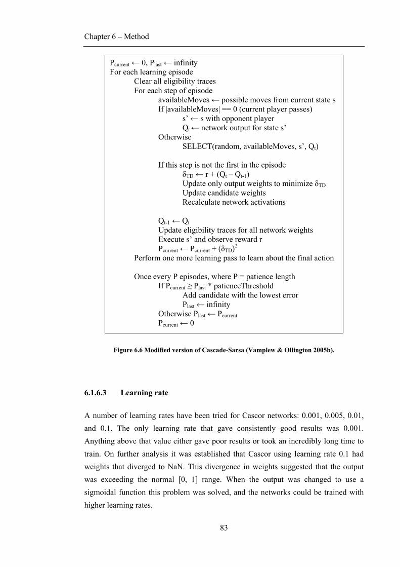
Chapter 6 – Method
83
Figure 6.6 Modified version of Cascade-Sarsa (Vamplew & Ollington 2005b).
6.1.6.3 Learning rate
A number of learning rates have been tried for Cascor networks: 0.001, 0.005, 0.01, and 0.1. The only learning rate that gave consistently good results was 0.001. Anything above that value either gave poor results or took an incredibly long time to train. On further analysis it was established that Cascor using learning rate 0.1 had weights that diverged to NaN. This divergence in weights suggested that the output was exceeding the normal [0, 1] range. When the output was changed to use a sigmoidal function this problem was solved, and the networks could be trained with higher learning rates.
Pcurrent ← 0, Plast ← infinity For each learning episode Clear all eligibility traces For each step of episode availableMoves ← possible moves from current state s If |availableMoves| == 0 (current player passes) s’ ← s with opponent player Qt ← network output for state s’ Otherwise
SELECT(random, availableMoves, s’, Qt) If this step is not the first in the episode δTD ← r + (Qt – Qt-1) Update only output weights to minimize δTD Update candidate weights Recalculate network activations Qt-1 ← Qt Update eligibility traces for all network weights Execute s’ and observe reward r Pcurrent ← Pcurrent + (δTD)2 Perform one more learning pass to learn about the final action Once every P episodes, where P = patience length If Pcurrent ≥ Plast * patienceThreshold Add candidate with the lowest error Plast ← infinity Otherwise Plast ← Pcurrent Pcurrent ← 0
Chapter 6 – Method
84
6.1.6.4 Number of candidates
The number of candidates is the number of units used to select a new hidden node.
This number was always set to 8 as used by (Vamplew & Ollington 2005b).
6.1.6.5 Maximum number of hidden nodes
This controls the maximum number of hidden nodes that can be added to the network.
As the MLPs used 30 hidden nodes, this number was also set to 30.
6.1.6.6 Patience threshold
The patience threshold controls how much the error is allowed to change before a new
hidden node is added. If currentError ≥ previousError x patienceThreshold then we
add a new hidden node. The patience threshold was always set to 0.95 as used by
(Vamplew & Ollington 2005b).
6.1.6.7 Patience length
The patience length is the minimum number of episodes that need to occur before a
new hidden node can be added. This number was adjusted such that the network
reaches the maximum number of hidden nodes before training is complete. For a
period of about 2,000 episodes the networks do not add any hidden nodes. After that
they add hidden nodes in a linear fashion, averaging about 833 episodes per hidden
node (~2.5 patience lengths). The networks reach their maximum capacity of 30
hidden nodes at about 27,000 episodes:
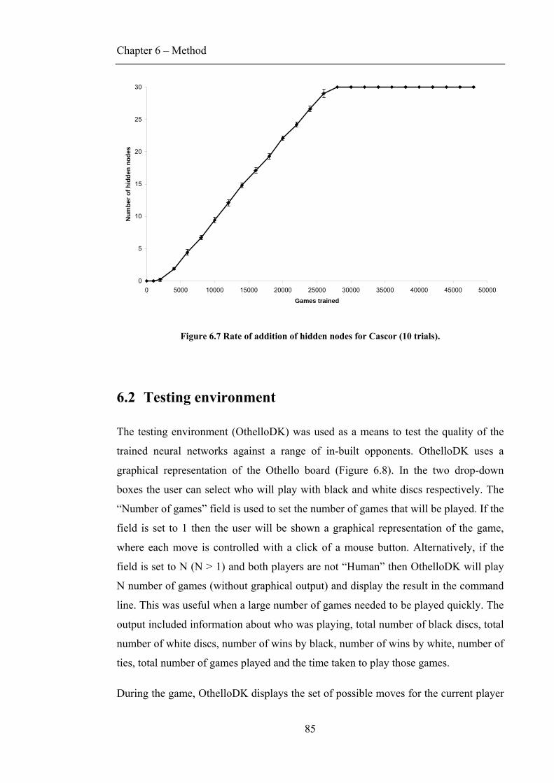
Chapter 6 – Method
85
0
5
10
15
20
25
30
0 5000 10000 15000 20000 25000 30000 35000 40000 45000 50000
Games trained
Num
ber o
f hid
den
node
s
Figure 6.7 Rate of addition of hidden nodes for Cascor (10 trials).
6.2 Testing environment
The testing environment (OthelloDK) was used as a means to test the quality of the
trained neural networks against a range of in-built opponents. OthelloDK uses a
graphical representation of the Othello board (Figure 6.8). In the two drop-down
boxes the user can select who will play with black and white discs respectively. The
“Number of games” field is used to set the number of games that will be played. If the
field is set to 1 then the user will be shown a graphical representation of the game,
where each move is controlled with a click of a mouse button. Alternatively, if the
field is set to N (N > 1) and both players are not “Human” then OthelloDK will play
N number of games (without graphical output) and display the result in the command
line. This was useful when a large number of games needed to be played quickly. The
output included information about who was playing, total number of black discs, total
number of white discs, number of wins by black, number of wins by white, number of
ties, total number of games played and the time taken to play those games.
During the game, OthelloDK displays the set of possible moves for the current player
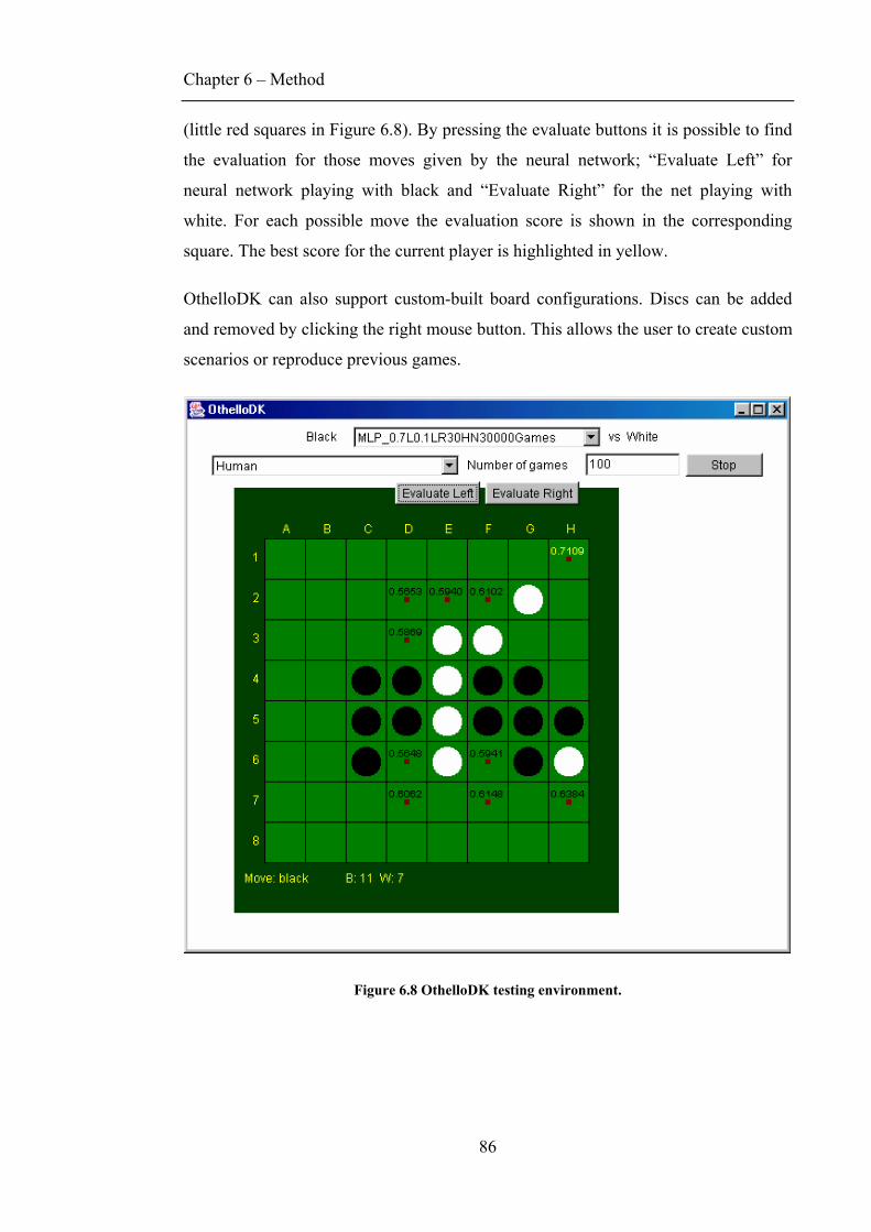
Chapter 6 – Method
86
(little red squares in Figure 6.8). By pressing the evaluate buttons it is possible to find
the evaluation for those moves given by the neural network; “Evaluate Left” for
neural network playing with black and “Evaluate Right” for the net playing with
white. For each possible move the evaluation score is shown in the corresponding
square. The best score for the current player is highlighted in yellow.
OthelloDK can also support custom-built board configurations. Discs can be added
and removed by clicking the right mouse button. This allows the user to create custom
scenarios or reproduce previous games.
Figure 6.8 OthelloDK testing environment.
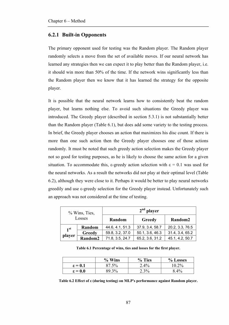
Chapter 6 – Method
87
6.2.1 Built-in Opponents
The primary opponent used for testing was the Random player. The Random player
randomly selects a move from the set of available moves. If our neural network has
learned any strategies then we can expect it to play better than the Random player, i.e.
it should win more than 50% of the time. If the network wins significantly less than
the Random player then we know that it has learned the strategy for the opposite
player.
It is possible that the neural network learns how to consistently beat the random
player, but learns nothing else. To avoid such situations the Greedy player was
introduced. The Greedy player (described in section 5.3.1) is not substantially better
than the Random player (Table 6.1), but does add some variety to the testing process.
In brief, the Greedy player chooses an action that maximizes his disc count. If there is
more than one such action then the Greedy player chooses one of those actions
randomly. It must be noted that such greedy action selection makes the Greedy player
not so good for testing purposes, as he is likely to choose the same action for a given
situation. To accommodate this, ε-greedy action selection with ε = 0.1 was used for
the neural networks. As a result the networks did not play at their optimal level (Table
6.2), although they were close to it. Perhaps it would be better to play neural networks
greedily and use ε-greedy selection for the Greedy player instead. Unfortunately such
an approach was not considered at the time of testing.
2nd player % Wins, Ties, Losses Random Greedy Random2
Random 44.6, 4.1, 51.3 37.9, 3.4, 58.7 20.2, 3.3, 76.5 Greedy 59.8, 3.2, 37.0 50.1, 3.6, 46.3 31.4, 3.4, 65.2 1st
player Random2 71.8, 3.5, 24.7 65.2, 3.6, 31.2 45.1, 4.2, 50.7
Table 6.1 Percentage of wins, ties and losses for the first player.
% Wins % Ties % Losses ε = 0.1 87.5% 2.4% 10.2% ε = 0.0 89.3% 2.3% 8.4%
Table 6.2 Effect of ε (during testing) on MLP's performance against Random player.
Chapter 6 – Method
88
Taking corners when they are available is an important part of winning in Othello.
Both Random and Greedy fail to do this and hence it was decided to introduce another
player – Random2. If there is a corner available then Random2 will take it, otherwise
it will choose a move randomly, just like the Random player. Random2 is
considerably better than both Random and Greedy players (Table 6.1).
6.2.2 Measuring learning
It is important to be able to evaluate the quality of the learned policy. Usually in
Reinforcement Learning problems, learning can be measured directly as the total
amount of received reward. However, this is not the case in a gaming context where
agents are trained through self-learning, because in these situations the accumulated
reward remains approximately constant. In such situations, the policy of the agent can
be evaluated by making it play against opponents whose abilities are known.
Sometimes the agent learns how to beat just one type of opponent and hence it is
important to test the agent against a range of opponents that have varying strategies.
The quality of a player can be measured as the likelihood of him winning against his
opponent. Since ties are possible in Othello they must also be taken into account. So a
better measure for a player’s quality would be the likelihood of him not losing against
his opponent.
Some authors (Leouski 1995; Moriarty & Miikkulainen 1995) have adopted the
following strategy for testing. Generate all the combinations of the first 4 legal moves
from the initial board configuration. Play a game from each of the 244 resulting board
states (60 unique states if we ignore rotations and reflections). However, it seems that
playing 244 games is not enough for meaningful statistical data. To prove this
hypothesis, 100 rounds of 244 games each were played between two Random players.
As the result of this experiment, the first player won 45.3% with a standard deviation
of 3.2%, while the second player won 50.5% with a standard deviation of 3.5%.
Based on the averages, we know that in a sample of many games the second player
will win more often than the first player. However in a sample of just 244 games,
statistically there is a 15.8% chance that the first player will win 48.5% or more, and a
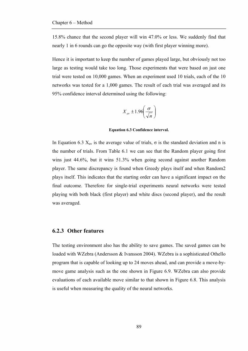
Chapter 6 – Method
89
15.8% chance that the second player will win 47.0% or less. We suddenly find that
nearly 1 in 6 rounds can go the opposite way (with first player winning more).
Hence it is important to keep the number of games played large, but obviously not too
large as testing would take too long. Those experiments that were based on just one
trial were tested on 10,000 games. When an experiment used 10 trials, each of the 10
networks was tested for a 1,000 games. The result of each trial was averaged and its
95% confidence interval determined using the following:
⎟⎟⎠
⎞⎜⎜⎝
⎛±
nX av
σ96.1
Equation 6.3 Confidence interval.
In Equation 6.3 Xav is the average value of trials, σ is the standard deviation and n is
the number of trials. From Table 6.1 we can see that the Random player going first
wins just 44.6%, but it wins 51.3% when going second against another Random
player. The same discrepancy is found when Greedy plays itself and when Random2
plays itself. This indicates that the starting order can have a significant impact on the
final outcome. Therefore for single-trial experiments neural networks were tested
playing with both black (first player) and white discs (second player), and the result
was averaged.
6.2.3 Other features
The testing environment also has the ability to save games. The saved games can be
loaded with WZebra (Andersson & Ivansson 2004). WZebra is a sophisticated Othello
program that is capable of looking up to 24 moves ahead, and can provide a move-by-
move game analysis such as the one shown in Figure 6.9. WZebra can also provide
evaluations of each available move similar to that shown in Figure 6.8. This analysis
is useful when measuring the quality of the neural networks.
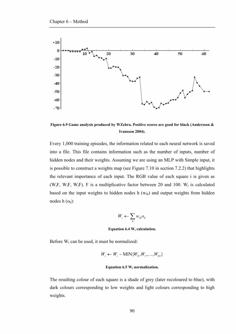
Chapter 6 – Method
90
Figure 6.9 Game analysis produced by WZebra. Positive scores are good for black (Andersson &
Ivansson 2004).
Every 1,000 training episodes, the information related to each neural network is saved
into a file. This file contains information such as the number of inputs, number of
hidden nodes and their weights. Assuming we are using an MLP with Simple input, it
is possible to construct a weights map (see Figure 7.10 in section 7.2.2) that highlights
the relevant importance of each input. The RGB value of each square i is given as
(WiF, WiF, WiF). F is a multiplicative factor between 20 and 100. Wi is calculated
based on the input weights to hidden nodes h (wih) and output weights from hidden
nodes h (oh):
∑←h
hihi owW
Equation 6.4 Wi calculation.
Before Wi can be used, it must be normalized:
},,,{MIN 6310 WWWWW ii K−←
Equation 6.5 Wi normalization.
The resulting colour of each square is a shade of grey (later recoloured to blue), with
dark colours corresponding to low weights and light colours corresponding to high
weights.
Chapter 7 – Results and Discussion
91
Chapter 7 Results and Discussion
7.1 MLP vs Cascade
In this section we compare the performance of MLP networks against Cascade
networks. To avoid any bias, both types of networks were trained with identical
parameters: Walker input scheme, softmax action selection, 30 hidden nodes, 50,000
training episodes and λ = 0.7. The only difference was in the learning rate, with
Cascade using 0.001 and MLP using 0.01. 10 trials of each type of network were
trained and tested against the Random player at intervals of 2,000 games (Figure 7.1).
The result for the first point (after 0 games trained) was obtained by playing Random
against Random; this is based on the assumption that the networks play completely
randomly at the start of training.
After the first 1,000 training episodes both networks improve equally to 60%, but
with a huge variation of ± 5%. After that, the performance of Cascade accelerates
rapidly, reaching a near-maximum of 80% after just 8,000 training episodes. In
contrast, the MLP network learns much slower, taking about 26,000 training episodes
to reach the same performance. After 26,000 training episodes the confidence
intervals of the networks overlap and we cannot conclude that one network is better
than the other. Due to its structure, Cascade uses less hidden nodes during the initial
training period. With fewer weights to adjust, Cascade is able to converge much faster
than MLP. One might wonder how the Cascade manages to reach good performance
with so few hidden nodes. In section 7.4 we show that the number of hidden nodes
does not affect performance.
As we increase the learning rate, the performance of Cascade stays the same, while
the performance of MLP improves (Figure 7.2). From Figure 7.2, we can see that
Cascade converges even faster than before (Figure 7.1), but its performance is poor
and very unstable, as indicated by long error bars. The performance of MLP on the
other hand is very consistent.
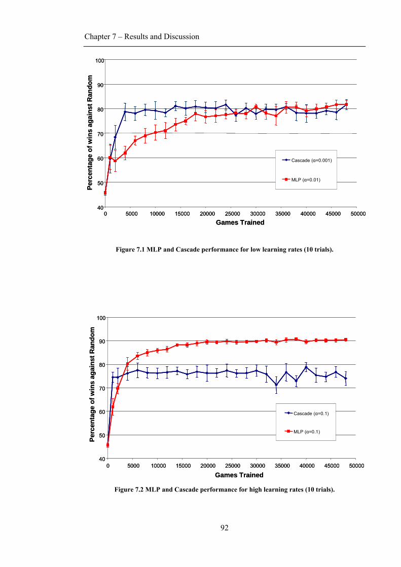
Chapter 7 – Results and Discussion
92
Figure 7.1 MLP and Cascade performance for low learning rates (10 trials).
Figure 7.2 MLP and Cascade performance for high learning rates (10 trials).
40
50
60
70
80
90
100
0 5000 10000 15000 20000 25000 30000 35000 40000 45000 50000
Games Trained
Perc
enta
ge o
f win
s ag
ains
t Ran
dom
Cascade (α=0.001)
MLP (α=0.01)
40
50
60
70
80
90
100
0 5000 10000 15000 20000 25000 30000 35000 40000 45000 50000
Games Trained
Perc
enta
ge o
f win
s ag
ains
t Ran
dom
Cascade (α=0.001)
MLP (α=0.01)
40
50
60
70
80
90
100
0 5000 10000 15000 20000 25000 30000 35000 40000 45000 50000
Games Trained
Perc
enta
ge o
f win
s ag
ains
t Ran
dom
Cascade (α=0.1)
MLP (α=0.1)
40
50
60
70
80
90
100
0 5000 10000 15000 20000 25000 30000 35000 40000 45000 50000
Games Trained
Perc
enta
ge o
f win
s ag
ains
t Ran
dom
Cascade (α=0.1)
MLP (α=0.1)

Chapter 7 – Results and Discussion
93
7.2 What did the networks learn?
In this section we analyse the networks’ learning ability. In particular, we show which
concepts the MLPs with Walker input have learnt and those that have eluded them. To
achieve this we use three methods: move evaluation, weights map and playing against
in-built opponents.
In move evaluation, the network is presented with a particular board, designed to test
its strengths and weaknesses. The network evaluates each available move, displaying
high values for good moves and low values for bad moves. The weights map
technique looks at the learned values for each square and is used to check the static
evaluation of the whole board. Finally, we play the networks against in-built
opponents to test their ability to generalize to different playing strategies.
7.2.1 Move evaluation
Consider Figure 7.3. The networks evaluate this position as highly winning for white.
We know from Figure 5.3 in section 5.3.1 that this is not true. The reason for this is
that the networks are trained with no look-ahead and hence they evaluate the board
statically. In this case, the white is given a high evaluation because he is controlling
important squares such as a-squares and b-squares. We also know that similarly-
matched opponents, like those used during self-play, are unlikely to experience such a
board position. So the networks are unlikely to evaluate it correctly.
The board position in Figure 7.4 was used by Cranney to determine whether the
networks have learned the mobility strategy (Cranney 2002). The best move for black
in this situation is E8, because then the white is left with just two moves (B2 and G2)
that both give away corners. Instead the network chooses H4.
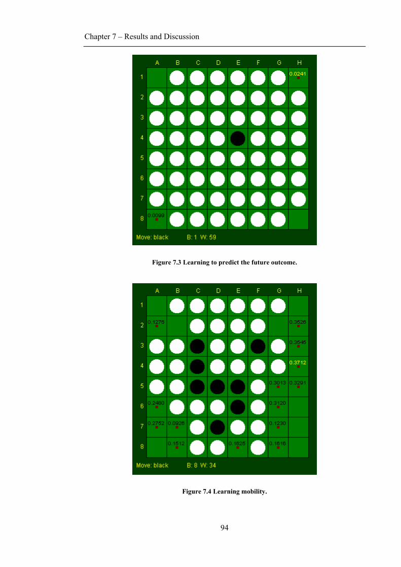
Chapter 7 – Results and Discussion
94
Figure 7.3 Learning to predict the future outcome.
Figure 7.4 Learning mobility.
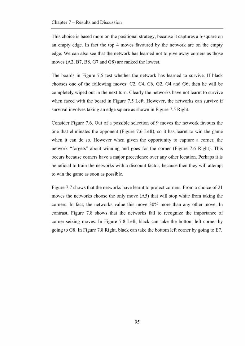
Chapter 7 – Results and Discussion
95
This choice is based more on the positional strategy, because it captures a b-square on
an empty edge. In fact the top 4 moves favoured by the network are on the empty
edge. We can also see that the network has learned not to give away corners as those
moves (A2, B7, B8, G7 and G8) are ranked the lowest.
The boards in Figure 7.5 test whether the network has learned to survive. If black
chooses one of the following moves: C2, C4, C6, G2, G4 and G6; then he will be
completely wiped out in the next turn. Clearly the networks have not learnt to survive
when faced with the board in Figure 7.5 Left. However, the networks can survive if
survival involves taking an edge square as shown in Figure 7.5 Right.
Consider Figure 7.6. Out of a possible selection of 9 moves the network favours the
one that eliminates the opponent (Figure 7.6 Left), so it has learnt to win the game
when it can do so. However when given the opportunity to capture a corner, the
network “forgets” about winning and goes for the corner (Figure 7.6 Right). This
occurs because corners have a major precedence over any other location. Perhaps it is
beneficial to train the networks with a discount factor, because then they will attempt
to win the game as soon as possible.
Figure 7.7 shows that the networks have learnt to protect corners. From a choice of 21
moves the networks choose the only move (A5) that will stop white from taking the
corners. In fact, the networks value this move 30% more than any other move. In
contrast, Figure 7.8 shows that the networks fail to recognize the importance of
corner-seizing moves. In Figure 7.8 Left, black can take the bottom left corner by
going to G8. In Figure 7.8 Right, black can take the bottom left corner by going to E7.
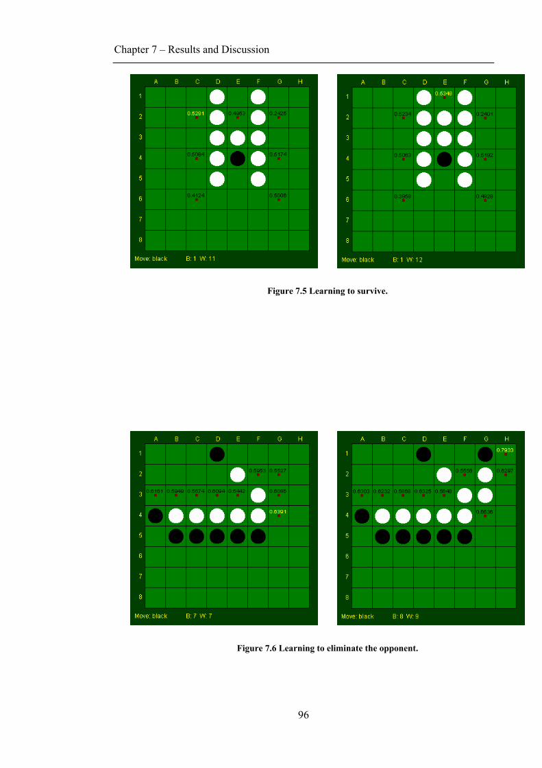
Chapter 7 – Results and Discussion
96
Figure 7.5 Learning to survive.
Figure 7.6 Learning to eliminate the opponent.
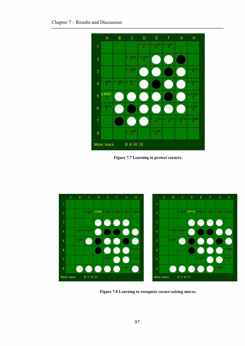
Chapter 7 – Results and Discussion
97
Figure 7.7 Learning to protect corners.
Figure 7.8 Learning to recognize corner-seizing moves.
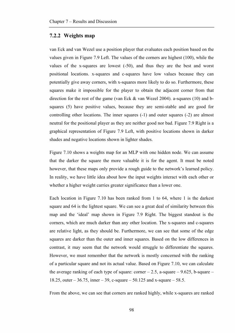
Chapter 7 – Results and Discussion
98
7.2.2 Weights map
van Eck and van Wezel use a position player that evaluates each position based on the
values given in Figure 7.9 Left. The values of the corners are highest (100), while the
values of the x-squares are lowest (-50), and thus they are the best and worst
positional locations. x-squares and c-squares have low values because they can
potentially give away corners, with x-squares more likely to do so. Furthermore, these
squares make it impossible for the player to obtain the adjacent corner from that
direction for the rest of the game (van Eck & van Wezel 2004). a-squares (10) and b-
squares (5) have positive values, because they are semi-stable and are good for
controlling other locations. The inner squares (-1) and outer squares (-2) are almost
neutral for the positional player as they are neither good nor bad. Figure 7.9 Right is a
graphical representation of Figure 7.9 Left, with positive locations shown in darker
shades and negative locations shown in lighter shades.
Figure 7.10 shows a weights map for an MLP with one hidden node. We can assume
that the darker the square the more valuable it is for the agent. It must be noted
however, that these maps only provide a rough guide to the network’s learned policy.
In reality, we have little idea about how the input weights interact with each other or
whether a higher weight carries greater significance than a lower one.
Each location in Figure 7.10 has been ranked from 1 to 64, where 1 is the darkest
square and 64 is the lightest square. We can see a great deal of similarity between this
map and the ‘ideal’ map shown in Figure 7.9 Right. The biggest standout is the
corners, which are much darker than any other location. The x-squares and c-squares
are relative light, as they should be. Furthermore, we can see that some of the edge
squares are darker than the outer and inner squares. Based on the low differences in
contrast, it may seem that the network would struggle to differentiate the squares.
However, we must remember that the network is mostly concerned with the ranking
of a particular square and not its actual value. Based on Figure 7.10, we can calculate
the average ranking of each type of square: corner – 2.5, a-square – 9.625, b-square –
18.25, outer – 36.75, inner – 39, c-square – 50.125 and x-square – 58.5.
From the above, we can see that corners are ranked highly, while x-squares are ranked

Chapter 7 – Results and Discussion
99
very low, closely followed by c-squares. The outer and inner squares are very
similarly ranked, although inner squares are ranked lower, which slightly contradicts
Figure 7.9 Left.
A B C D E F G H
1 100 -20 10 5 5 10 -20 100
2 -20 -50 -2 -2 -2 -2 -50 -20
3 10 -2 -1 -1 -1 -1 -2 10
4 5 -2 -1 -1 -1 -1 -2 5
5 5 -2 -1 -1 -1 -1 -2 5
6 10 -2 -1 -1 -1 -1 -2 10
7 -20 -50 -2 -2 -2 -2 -50 20
8 100 -20 10 5 5 10 -20 100
Figure 7.9 Positional strategy. Left: square values based on (van Eck & van Wezel 2004).
Right: values on the left converted to a weights map.
Figure 7.10 Weights map learned by MLP with Advanced input (1 trial).
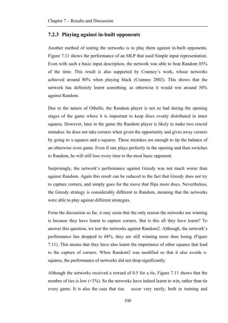
Chapter 7 – Results and Discussion
100
7.2.3 Playing against in-built opponents
Another method of testing the networks is to play them against in-built opponents.
Figure 7.11 shows the performance of an MLP that used Simple input representation.
Even with such a basic input description, the network was able to beat Random 85%
of the time. This result is also supported by Cranney’s work, whose networks
achieved around 80% when playing black (Cranney 2002). This shows that the
network has definitely learnt something, as otherwise it would win around 50%
against Random.
Due to the nature of Othello, the Random player is not so bad during the opening
stages of the game where it is important to keep discs evenly distributed in inner
squares. However, later in the game the Random player is likely to make two crucial
mistakes: he does not take corners when given the opportunity and gives away corners
by going to x-squares and c-squares. These mistakes are enough to tip the balance of
an otherwise even game. Even if one plays perfectly in the opening and then switches
to Random, he will still lose every time to the most basic opponent.
Surprisingly, the network’s performance against Greedy was not much worse than
against Random. Again this result can be reduced to the fact that Greedy does not try
to capture corners, and simply goes for the move that flips more discs. Nevertheless,
the Greedy strategy is considerably different to Random, meaning that the networks
were able to play against different strategies.
From the discussion so far, it may seem that the only reason the networks are winning
is because they have learnt to capture corners. But is this all they have learnt? To
answer this question, we test the networks against Random2. Although, the network’s
performance has dropped to 68%, they are still winning more than losing (Figure
7.11). This means that they have also learnt the importance of other squares that lead
to the capture of corners. When Random2 was modified so that it also avoids x-
squares, the performance of networks did not drop significantly.
Although the networks received a reward of 0.5 for a tie, Figure 7.11 shows that the
number of ties is low (<3%). So the networks have indeed learnt to win, rather than tie
every game. It is also the case that ties occur very rarely, both in training and
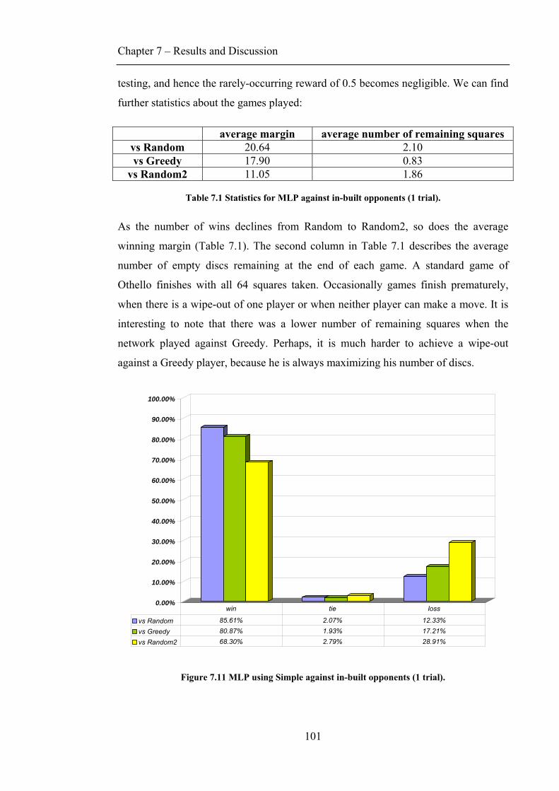
Chapter 7 – Results and Discussion
101
testing, and hence the rarely-occurring reward of 0.5 becomes negligible. We can find
further statistics about the games played:
average margin average number of remaining squares vs Random 20.64 2.10 vs Greedy 17.90 0.83
vs Random2 11.05 1.86
Table 7.1 Statistics for MLP against in-built opponents (1 trial).
As the number of wins declines from Random to Random2, so does the average
winning margin (Table 7.1). The second column in Table 7.1 describes the average
number of empty discs remaining at the end of each game. A standard game of
Othello finishes with all 64 squares taken. Occasionally games finish prematurely,
when there is a wipe-out of one player or when neither player can make a move. It is
interesting to note that there was a lower number of remaining squares when the
network played against Greedy. Perhaps, it is much harder to achieve a wipe-out
against a Greedy player, because he is always maximizing his number of discs.
0.00%
10.00%
20.00%
30.00%
40.00%
50.00%
60.00%
70.00%
80.00%
90.00%
100.00%
vs Random 85.61% 2.07% 12.33%vs Greedy 80.87% 1.93% 17.21%vs Random2 68.30% 2.79% 28.91%
win tie loss
Figure 7.11 MLP using Simple against in-built opponents (1 trial).
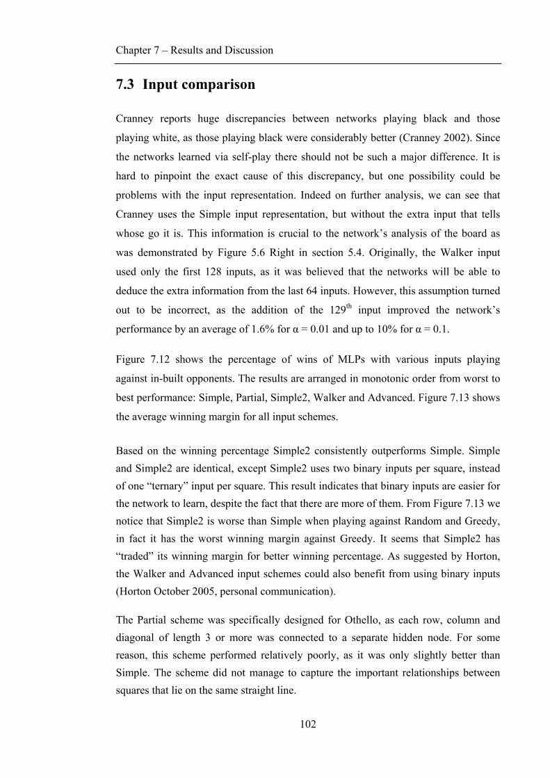
Chapter 7 – Results and Discussion
102
7.3 Input comparison
Cranney reports huge discrepancies between networks playing black and those
playing white, as those playing black were considerably better (Cranney 2002). Since
the networks learned via self-play there should not be such a major difference. It is
hard to pinpoint the exact cause of this discrepancy, but one possibility could be
problems with the input representation. Indeed on further analysis, we can see that
Cranney uses the Simple input representation, but without the extra input that tells
whose go it is. This information is crucial to the network’s analysis of the board as
was demonstrated by Figure 5.6 Right in section 5.4. Originally, the Walker input
used only the first 128 inputs, as it was believed that the networks will be able to
deduce the extra information from the last 64 inputs. However, this assumption turned
out to be incorrect, as the addition of the 129th input improved the network’s
performance by an average of 1.6% for α = 0.01 and up to 10% for α = 0.1.
Figure 7.12 shows the percentage of wins of MLPs with various inputs playing
against in-built opponents. The results are arranged in monotonic order from worst to
best performance: Simple, Partial, Simple2, Walker and Advanced. Figure 7.13 shows
the average winning margin for all input schemes.
Based on the winning percentage Simple2 consistently outperforms Simple. Simple and Simple2 are identical, except Simple2 uses two binary inputs per square, instead of one “ternary” input per square. This result indicates that binary inputs are easier for the network to learn, despite the fact that there are more of them. From Figure 7.13 we notice that Simple2 is worse than Simple when playing against Random and Greedy, in fact it has the worst winning margin against Greedy. It seems that Simple2 has “traded” its winning margin for better winning percentage. As suggested by Horton, the Walker and Advanced input schemes could also benefit from using binary inputs (Horton October 2005, personal communication).
The Partial scheme was specifically designed for Othello, as each row, column and diagonal of length 3 or more was connected to a separate hidden node. For some reason, this scheme performed relatively poorly, as it was only slightly better than Simple. The scheme did not manage to capture the important relationships between squares that lie on the same straight line.

Chapter 7 – Results and Discussion
103
The Walker input was the best input from those that were not given any extra strategic
information. The performance of Walker input is close to that of Advanced in both
winning percentage and winning margin. We conclude that its superiority against
simple inputs is due to the extra 64 “look-ahead” inputs.
It was no surprise that Advanced was the best input scheme. Its dominance is
primarily due to the mobility information that it received. When playing against in-
built opponents it often restricted their mobility, forcing them to give away corners.
Once it took control of corners, it ensured that the opponent had to pass, thus
maximizing its own disc count. We also notice that Walker and Advanced inputs have
the strongest generalization skills as they have the least decline in performance
(Figure 7.12).
0.00%
10.00%
20.00%
30.00%
40.00%
50.00%
60.00%
70.00%
80.00%
90.00%
100.00%
Simple 85.61% 80.87% 68.30%Partial 86.59% 85.80% 74.49%Simple2 88.15% 86.52% 78.46%Walker 91.77% 89.88% 84.97%Advanced 93.51% 90.36% 86.72%
vs Random vs Greedy vs Random2
Figure 7.12 MLPs with various inputs against in-built opponents (1 trial).
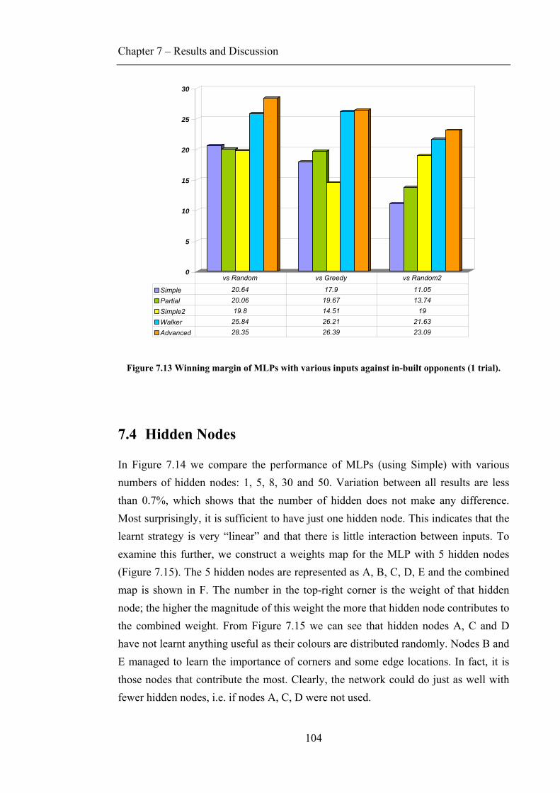
Chapter 7 – Results and Discussion
104
0
5
10
15
20
25
30
Simple 20.64 17.9 11.05Partial 20.06 19.67 13.74Simple2 19.8 14.51 19Walker 25.84 26.21 21.63Advanced 28.35 26.39 23.09
vs Random vs Greedy vs Random2
Figure 7.13 Winning margin of MLPs with various inputs against in-built opponents (1 trial).
7.4 Hidden Nodes
In Figure 7.14 we compare the performance of MLPs (using Simple) with various numbers of hidden nodes: 1, 5, 8, 30 and 50. Variation between all results are less than 0.7%, which shows that the number of hidden does not make any difference. Most surprisingly, it is sufficient to have just one hidden node. This indicates that the learnt strategy is very “linear” and that there is little interaction between inputs. To examine this further, we construct a weights map for the MLP with 5 hidden nodes (Figure 7.15). The 5 hidden nodes are represented as A, B, C, D, E and the combined map is shown in F. The number in the top-right corner is the weight of that hidden node; the higher the magnitude of this weight the more that hidden node contributes to the combined weight. From Figure 7.15 we can see that hidden nodes A, C and D have not learnt anything useful as their colours are distributed randomly. Nodes B and E managed to learn the importance of corners and some edge locations. In fact, it is those nodes that contribute the most. Clearly, the network could do just as well with fewer hidden nodes, i.e. if nodes A, C, D were not used.
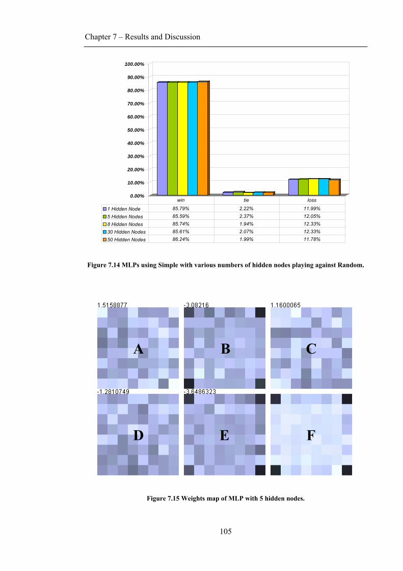
Chapter 7 – Results and Discussion
105
0.00%
10.00%
20.00%
30.00%
40.00%
50.00%
60.00%
70.00%
80.00%
90.00%
100.00%
1 Hidden Node 85.79% 2.22% 11.99%5 Hidden Nodes 85.59% 2.37% 12.05%8 Hidden Nodes 85.74% 1.94% 12.33%30 Hidden Nodes 85.61% 2.07% 12.33%50 Hidden Nodes 86.24% 1.99% 11.78%
win tie loss
Figure 7.14 MLPs using Simple with various numbers of hidden nodes playing against Random.
Figure 7.15 Weights map of MLP with 5 hidden nodes.
A B C
D E F

Chapter 7 – Results and Discussion
106
7.5 Sarsa(λ) vs Q-Learning(λ)
To compare the training algorithms and MLP using Simple input was trained with
both Sarsa(λ) and Q-Learning(λ). The results are shown in Figure 7.16. Clearly the
training algorithm did not make any impact on the final performance. A more
noticeable difference is observed when the training algorithms are compared based on
their learning curve (Figure 7.17). From Figure 7.17 we can see that Sarsa(λ)
converges faster but is very unstable, while Q-Learning(λ) is slow and consistent.
Whenever an exploratory action is chosen in Q-learning(λ), the eligibility traces for
all previous states are reset to zero, which should slow down the flow of information
from terminating states to initial states. This is particularly true in early episodes,
where we are choosing more exploratory actions. In Sarsa(λ) there is more variability
in the values being learnt, as we learn from both exploratory and greedy actions.
Therefore, if we have a large number of poor exploratory actions then this could
reduce the quality of the policy (Dr. Vamplew October 2005, personal
communication).
0.00%
10.00%
20.00%
30.00%
40.00%
50.00%
60.00%
70.00%
80.00%
90.00%
100.00%
Q-Learning(λ) 85.88% 80.58% 68.39%Sarsa(λ) 85.61% 80.87% 68.30%
vs Random vs Greedy vs Random2
Figure 7.16 MLPs using Q-Learning and Sarsa against in-built opponents (1 trial).
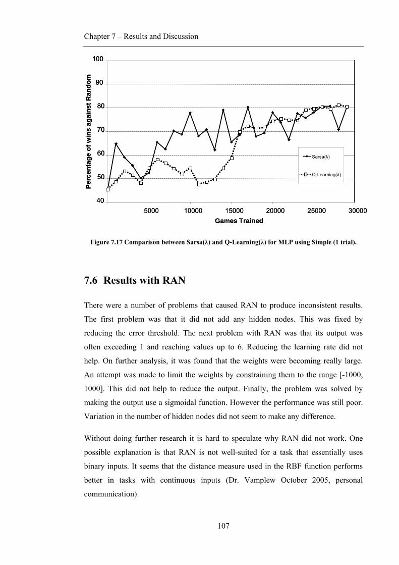
Chapter 7 – Results and Discussion
107
40
50
60
70
80
90
100
5000 10000 15000 20000 25000 30000Games Trained
Perc
enta
ge o
f win
s ag
ains
t Ran
dom
Sarsa(λ)
Q-Learning(λ)
40
50
60
70
80
90
100
40
50
60
70
80
90
100
5000 10000 15000 20000 25000 30000Games Trained
Perc
enta
ge o
f win
s ag
ains
t Ran
dom
Sarsa(λ)
Q-Learning(λ)
Figure 7.17 Comparison between Sarsa(λ) and Q-Learning(λ) for MLP using Simple (1 trial).
7.6 Results with RAN
There were a number of problems that caused RAN to produce inconsistent results.
The first problem was that it did not add any hidden nodes. This was fixed by
reducing the error threshold. The next problem with RAN was that its output was
often exceeding 1 and reaching values up to 6. Reducing the learning rate did not
help. On further analysis, it was found that the weights were becoming really large.
An attempt was made to limit the weights by constraining them to the range [-1000,
1000]. This did not help to reduce the output. Finally, the problem was solved by
making the output use a sigmoidal function. However the performance was still poor.
Variation in the number of hidden nodes did not seem to make any difference.
Without doing further research it is hard to speculate why RAN did not work. One
possible explanation is that RAN is not well-suited for a task that essentially uses
binary inputs. It seems that the distance measure used in the RBF function performs
better in tasks with continuous inputs (Dr. Vamplew October 2005, personal
communication).

Chapter 8 – Conclusion and Future Work
108
Chapter 8 Conclusion and Future Work
8.1 MLP vs Cascade
For slower learning rates, Cascade converges faster than MLP. The reason for this is
that Cascade uses less hidden nodes during training. Its policy is not greatly affected,
because the number of hidden nodes does not make any difference. Despite having
faster convergence, Cascade does not actually reach better performance.
For faster learning rates, Cascade stays the same, while the MLP converges to a much
better policy. The fact that Cascade works better with smaller learning rates is also
supported by (Vamplew & Ollington 2005b). Since the number of weights in Cascade
is increasing, it seems appropriate that its learning rate should also increase. Future
work could investigate the effects of starting with α = 0.001 and increasing it towards
0.1 every time a new node is added.
Vamplew and Ollington show that Cascade-Sarsa outperforms MLP on Acrobot and
Mountain-Car, but not on the Puddleworld task (Vamplew & Ollington 2005b). A
possible explanation is that in Puddleworld the puddles are convex polygons and
hence require more than one hidden node to learn. Cascade-Sarsa does not meet this
requirement because it adds just one node at a time. Cascade-Sarsa can be improved
by training triplets of candidate nodes and then adding all three nodes to the network.
Although this is likely to give better results on Puddleworld, it will probably not help
much in Othello.
8.2 Learned knowledge
In summary, the networks did not learn how to:
• Play using the mobility strategy
• Predict the future outcome
• Avoid being eliminated (survival)
Chapter 8 – Conclusion and Future Work
109
• Recognize corner-seizing moves
As discussed in section 5.3.3, mobility is an exceptionally difficult strategy to learn,
even for human players. It requires a deep understanding of the game and is not
evident from a straightforward examination. Clearly, we cannot expect the networks
to learn mobility without providing them with extra information, such as the count of
the available moves.
The next three items on the list are related, in that they all require a certain amount of
look-ahead. Predicting the final outcome in a situation like in Figure 7.3 is not easy,
because a number of major changes occur in those last moves. It is hard for networks
to learn to avoid being eliminated, because for them it is simply another loss, without
any features that distinguish it from other losses. Again, discounting techniques could
be useful for such situations.
Given the fact that the networks learned the importance of corners and ways of
protecting them, it was a surprise that they didn’t learn to recognize corner-seizing
moves. Similarly, it was surprising that the networks were able to eliminate the
opponent, but unable to survive. Since these notions are exact opposites, a network
that was trained by self-play should have either learnt both or none. In other words,
this is the same as learning that 2 + 3 = 5, but not being able to see that 3 + 2 = 5. One
possible explanation is that the learned value of a given board is not completely
symmetric with respect to each player. Below we define the symmetry value:
)(value)(value)(symmetry 1−+= sss WB
Equation 8.1 Symmetry value of a given board s.
In Equation 8.1, valueB(s) represents the value of the board s evaluated from black’s
perspective; valueW(s-1) represents the value of the board s with inverted colours,
evaluated from white’s perspective. Now we will define the symmetry property for a
game G: if G has the symmetry property then symmetry(s) = 1 for all s that occur in
G. The symmetry property was tested by playing an MLP with Walker input against
Random for 1,000 games. Figure 8.1 shows the average symmetry value for each
stage in the game:
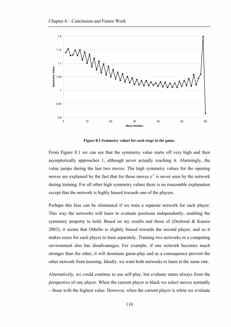
Chapter 8 – Conclusion and Future Work
110
0.9
0.95
1
1.05
1.1
1.15
1.2
0 10 20 30 40 50 60
Move Number
Sym
met
ry V
alue
Figure 8.1 Symmetry values for each stage in the game.
From Figure 8.1 we can see that the symmetry value starts off very high and then
asymptotically approaches 1, although never actually reaching it. Alarmingly, the
value jumps during the last two moves. The high symmetry values for the opening
moves are explained by the fact that for those moves s-1 is never seen by the network
during training. For all other high symmetry values there is no reasonable explanation
except that the network is highly biased towards one of the players.
Perhaps this bias can be eliminated if we train a separate network for each player.
This way the networks will learn to evaluate positions independently, enabling the
symmetry property to hold. Based on my results and those of (Deshwal & Kasera
2003), it seems that Othello is slightly biased towards the second player, and so it
makes sense for each player to train separately. Training two networks in a competing
environment also has disadvantages. For example, if one network becomes much
stronger than the other, it will dominate game-play and as a consequence prevent the
other network from learning. Ideally, we want both networks to learn at the same rate.
Alternatively, we could continue to use self-play, but evaluate states always from the
perspective of one player. When the current player is black we select moves normally
– those with the highest value. However, when the current player is white we evaluate
Chapter 8 – Conclusion and Future Work
111
his position from black’s perspective by reversing the colours on the board. This way
both selections are made from black’s perspective with high values corresponding to
good moves.
Despite the negative results, the networks did manage to learn:
• The importance of edge locations, especially corners
• The negative outcome of going to x-squares and c-squares
• How to protect corners
• How to eliminate the opponent
The first two points show that the networks learned the positional strategy, which
involves the correct evaluation of each board location. In particular the networks did
really well in learning the importance of corners and ranked them 1, 2, 3 and 4 (see
Figure 7.10 in section 7.2.2). However, they did not do as well for x-squares, ranking
them 52, 57, 62 and 64. The bottom-left x-square (52) can cause problems, as the
networks will go to that square unnecessarily often.
The last two points are of particular interest, because they show that the networks
have learned more than just the positional strategy. Protecting corners and eliminating
the opponent are relatively complex strategies to learn.
8.3 Input representation
It was found that Simple2 outperforms Simple. This indicates that binary inputs are easier to learn. We can expect further improvement if binary inputs are used for other inputs representations. Partial input does not perform well. Future work can involve applying partial input to Cascade. To achieve this, the Cascade networks will need to start with all the partial hidden nodes in place and add more nodes during training. Variations to the Partial input are also possible. For example, we can add hidden nodes for each block of 3x3 and 2x5 squares. This strategy was used with great success in LOGISTELLO (Buro 1994).
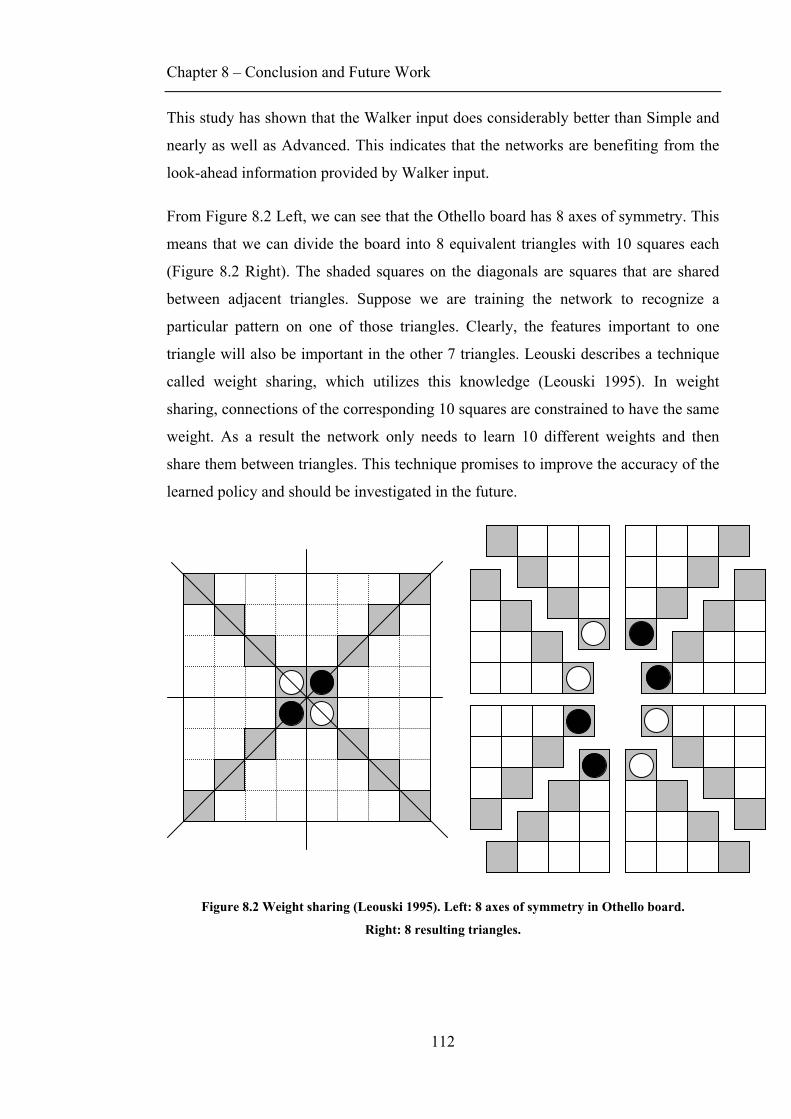
Chapter 8 – Conclusion and Future Work
112
This study has shown that the Walker input does considerably better than Simple and
nearly as well as Advanced. This indicates that the networks are benefiting from the
look-ahead information provided by Walker input.
From Figure 8.2 Left, we can see that the Othello board has 8 axes of symmetry. This
means that we can divide the board into 8 equivalent triangles with 10 squares each
(Figure 8.2 Right). The shaded squares on the diagonals are squares that are shared
between adjacent triangles. Suppose we are training the network to recognize a
particular pattern on one of those triangles. Clearly, the features important to one
triangle will also be important in the other 7 triangles. Leouski describes a technique
called weight sharing, which utilizes this knowledge (Leouski 1995). In weight
sharing, connections of the corresponding 10 squares are constrained to have the same
weight. As a result the network only needs to learn 10 different weights and then
share them between triangles. This technique promises to improve the accuracy of the
learned policy and should be investigated in the future.
Figure 8.2 Weight sharing (Leouski 1995). Left: 8 axes of symmetry in Othello board.
Right: 8 resulting triangles.
Chapter 8 – Conclusion and Future Work
113
8.4 Comparison to other Othello programs
Our agent performs similar to other TD-based Othello programs. Using Simple
representation our networks perform 6% better than those of Cranney. Although
Cranney also uses Simple, he does not provide whose move it is, which decreases the
performance of his networks.
The networks trained by Walker et al. tend to beat Windows Reversi at the Novice
(2nd level), but tend to lose to Expert (3rd level). Our networks trained with Walker
representation played a series of 10 games against each level of Windows Reversi
(Table 8.1). Note that it was not feasible to play more games, because the source code
for Windows Reversi is not publicly available. The results in Table 8.1 mirror those
reported by Walker et al. Interestingly, the networks play better against Novice (2nd
level) than Beginner (1st level). Perhaps the networks have learned how to beat a more
advanced player like Novice, but at the same time unlearned how to beat Beginner.
Wins Ties Losses vs Beginner 6 0 4 vs Novice 8 0 2 vs Expert 2 1 7
Table 8.1 MLP using Walker against Windows Reversi.
Not surprisingly our networks perform poorly when compared to other more
sophisticated programs (Deshwal & Kasera 2003; Leouski 1995; Tournavitis 2003).
But this is mainly because other studies heavily rely on move look-ahead to create a
stronger player. For example during the middle game, Leouski uses 2-ply search,
Deshwal et al. use 4-ply search and Tournavitis uses 8-ply. Furthermore, Leouski uses
exhaustive search for the last 10 moves, Deshwal et al. and Tournavitis use exhaustive
search for the last 16 moves.
8.5 Number of hidden nodes
This study has shown that the number of hidden nodes in neural networks makes little
difference to the performance. In fact this is one of the reasons why Cascade

Chapter 8 – Conclusion and Future Work
114
converges faster than MLP. It also means that the learned strategy is rather linear.
This can be improved by using a certain amount of look-ahead during training. It is
also possible that 8 x 8 Othello is too complex for the networks to learn input
dependencies. Future work can investigate applying these techniques to 6 x 6 Othello,
as used by (Yoshioka et al. 1999).
8.6 Further improvements
In Othello there are at least three distinct stages in the game: opening, middle and
end-game. Each stage lasts approximately 20 moves and requires a separate strategy.
During the opening, play is generally centred on the middle squares. Stability and
mobility play an important role during the middle stage, whereas the number of discs
is the main factor in the end-game. We can provide extra input that describes the
current stage of the game. Alternatively we can train three different networks, one for
each stage, as suggested by (Leouski 1995). Furthermore, the number of game stages
can be increased. For example, some authors use as many as 12 game stages
(Tournavitis 2003).
Ghory suggests that an agent learns better when playing against an opponent that is
stronger than itself (Ghory 2004). This way the stronger opponent can teach the agent
– an approach similar to supervised learning. To achieve this, we can apply shaping
(introduced in section 4.9.1). The agent can start by playing against Random. Once it
has learned to beat Random, it can be trained against Greedy, Random2 and other
more advanced opponents. An opponent can also be created by introducing game-tree
search to the current agent (Ghory 2004).
Chapter 9 – References
115
Chapter 9 References
Alliot, JM & Durand, N 1996, 'A genetic algorithm to improve an Othello program', Artificial Evolution, vol. 1063, pp. 307-19.
Allis, LV 1988, 'A knowledge-based approach of Connect Four: The game is over, white to move wins', M.Sc. thesis, Vrije Universiteit.
Allis, LV 1994, 'Searching for solutions in games and artificial intelligence', PhD thesis, University of Limburg.
Allis, LV, van den Herik, HJ & Huntjens, MPH 1995, 'Go-Moku solved by new search techniques', Computational Intelligence, vol. 12, no. 1, pp. 7-24.
Anderson, CW 1986, 'Learning and Problem Solving with Multilayer Connectionist Systems', PhD thesis, University of Massachusetts.
Andersson, G & Ivansson, L 2004, WZebra, 4.2.2 beta 1 edn.
Beal, DF & Smith, MC 1997, 'Learning piece values using temporal differences', ICCA Journal, vol. 20, no. 3, pp. 147-51.
Beal, DF & Smith, MC 1999, 'First results from using temporal difference learning in Shogi', Computers and Games, vol. 1558, pp. 113-25.
Beal, DF & Smith, MC 2000, 'Temporal difference learning for heuristic search and game playing', Information Sciences, vol. 122, no. 1, pp. 3-21.
Beale, R & Jackson, T 1992, Neural Computing: An Introduction, Institute of Physics Publishing, Bristol and Philadelphia.
Bellemare, MG, Precup, D & Rivest, F 2004, Reinforcement Learning Using Cascade-Correlation Neural Networks, McGill University, Canada.
Billman, D & Shaman, D 1990, 'Strategy Knowledge and Strategy Change in Skilled Performance - a Study of the Game Othello', American Journal of Psychology, vol. 103, no. 2, pp. 145-66.
Boyan, JA & Moore, AW 1995, 'Generalization in reinforcement learning: safely approximating the value function', Advances in Neural Information Processing Systems, vol. 7, pp. 369-76.
Brockington, MG 1998, 'Asynchronous parallel game-tree search', PhD thesis, University of Alberta.
Buro, M 1994, 'Logistello - a strong learning Othello program', paper presented to 19th Annual Conference Gesellschaft fur Klassifikation.
Buro, M 1995, 'Probcut - an Effective Selective Extension of the Alpha-Beta Algorithm', ICCA Journal, vol. 18, no. 2, pp. 71-6.
Buro, M 2003, 'The evolution of strong Othello programs', Entertainment Computing - Technology and Applications, pp. 81-8.
Chellapilla, K & Fogel, DB 1999, 'Evolving neural networks to play Checkers without relying on expert knowledge', IEEE Transactions on Neural Networks, vol. 10, no. 6, pp. 1382-91.

Chapter 9 – References
116
Chellapilla, K & Fogel, DB 2001, 'Evolving an expert Checkers playing program without using human expertise', IEEE Transactions on Evolutionary Computation, vol. 5, no. 4, pp. 422-8.
Clouse, J 1992, Wystan.
Cranney, PJ 2002, 'A comparison of self-play versus tournament-play in applying reinforcement learning to game playing', Honours thesis, University of Tasmania.
Crites, RH & Barto, AG 1996, 'Improving Elevator Performance Using Reinforcement Learning', paper presented to Advances in Neural Information Processing Systems 8.
Dazeley, R 2001, 'Investigations into playing Chess endgames using reinforcement learning', Honours thesis, University of Tasmania.
Deshwal, PS & Kasera, V 2003, Caesar - An Othello Program, Stanford University.
Donkers, HHLM, de Voogt, A & Uiterwijk, JWHM 2000, 'Human versus machine problem-solving: winning openings in Dakon', Board games studies, vol. 3, pp. 79-88.
Eiben, AE & Smith, JE 2003, Introduction to evolutionary computing, Springer-Verlag Berlin.
Ekker, R, van der Werf, ECD & Schomaker, LRB 2004, 'Dedicated TD-learning for stronger gameplay: applications to Go', Proceedings of Benelearn 2004 Annual Machine Learning Conference of Belgium and The Netherlands, pp. 46-52.
Fahlman, SE 1988, 'Faster-learning variations on Back-propagation: An empirical study', paper presented to Proceedings of the 1988 Connectionist Models Summer School.
Fahlman, SE & Lebiere, C 1990, 'The Cascade-Correlation Learning Architecture', in Touretzky (ed.), Advances in Neural Information Processing II, Morgan Kauffman, San Mateo, California, pp. 524-32.
Feinstein, J 1993, 'Amenor wins world 6 x 6 champtionships!' British Othello Federation Newsletter, pp. 6-9.
Fogel, DB 2000, 'Evolving a Checkers player without relying on human expertise', Intelligence, vol. 11, no. 2, pp. 20-7.
Fogel, DB, Hays, TJ, Hahn, SL & Quon, J 2004, 'A self-learning evolutionary Chess program', paper presented to Proceedings of the IEEE, DEC.
Gasser, RU 1996, 'Solving Nine-Men's-Morris', in RJ Nowakowski (ed.), Games of no chance, Cambridge University Press, Cambridge, USA, pp. 101-13.
Ghory, I 2004, 'Reinforcement learning in board games', Masters thesis, University of Bristol.
Gosavi, A, Bandla, N & Das, TK 2002, 'A reinforcement learning approach to a single leg airline revenue management problem with multiple fare classes and overbooking', IIE Transactions, vol. 9, pp. 729-42.
Hebb, DO 1949, The Organization of Behaviour, John Wiley & Sons, New York.
Irving, G, Donkers, HHLM & Uiterwijk, JWHM 2000, 'Solving Kalah', ICGA Journal, vol. 23, no. 3, pp. 139-47.
Chapter 9 – References
117
Kaelbling, LP, Littman, ML & Moore, AW 1996, 'Reinforcement Learning: A Survey', Journal of Artificial Intelligence Research, vol. 4, pp. 237-85.
Koenig, S & Simmons, R 1996, 'The Effect of Representation and Knowledge on Goal-Directed Exploration with Reinforcement Learning Algorithms', Machine Learning, no. 22, pp. 227-50.
Lahnajarvi, JJT, Lehtokangas, MI & Saarinen, JPP 2002, 'Evaluation of constructive neural networks with cascaded architectures', Neurocomputing, vol. 48, pp. 573-607.
Lang, KJ & Witbrock, MJ 1988, 'Learning to tell two spirals apart', paper presented to Proceedings of the 1988 Connectionist Models Summer School.
Lee, KF & Mahajan, S 1990, 'The Development of a World Class Othello Program', Artificial Intelligence, vol. 43, no. 1, pp. 21-36.
Leouski, A 1995, 'Learning of Position Evaluation in the Game of Othello', Masters thesis, University of Massachusetts.
McClelland, JL & Rumelhart, DE 1986, Parallel Distributed Processing, MIT Press, Cambridge, MA.
McCulloch, WS & Pitts, W 1943, 'A logical calculus of the ideas immanent in nervous activity', Bulletin of Mathematical Biophysics, vol. 5, pp. 115-33.
Minsky, M & Papert, SA 1969, Perceptrons: An Introduction to Computational Geometry, MIT Press, Cambridge, MA.
Mitchell, TM 1997, 'Artificial neural networks', in Machine Learning, McGraw Hill.
Moriarty, DE & Miikkulainen, R 1995, 'Discovering Complex Othello Strategies through Evolutionary Neural Networks', Connection Science, vol. 7, no. 3, pp. 195-209.
Parker, DB 1985, Learning logic, 47, Center for Computational Research in Economics and Management Science, MIT.
Pednault, E, Abe, N & Zadrozny, B 2002, 'Sequential cost-sensitive decision making with reinforcement learning', Proceedings of the Eighth International Conference on Knowledge Discovery and Data Mining, pp. 259-68.
Platt, J 1991, 'A resource-allocating network for function interpolation', Neural Computation, vol. 3, no. 2, pp. 213-25.
Pollack, JB & Blair, AD 1997, 'Why did TD-Gammon work?' Advances in Neural Information Processing Systems 9, pp. 10-6.
Prechelt, L 1997, 'Investigation of the CasCor family of learning algorithms', Neural Networks, vol. 10, no. 5, pp. 885-96.
Randlov, J & Alstrom, P 1998, 'Learning to Drive a Bicycle using Reinforcement Learning and Shaping', paper presented to Fifteenth International Conference in Machine Learning.
Richards, N, Moriarty, DE & Miikkulainen, R 1998, 'Evolving neural networks to play Go', Applied Intelligence, vol. 8, no. 1, pp. 85-96.
Rivest, F & Precup, D 2003, 'Combining TD-learning with Cascade-correlation Networks', paper presented to Twentieth International Conference on Machine Learning, Washington DC.
Chapter 9 – References
118
Rosenblatt, F 1962, Principles of Neurodynamics, Spartan, New York.
Rosenbloom, PS 1982, 'World-championship-level Othello program', Artificial Intelligence, vol. 19, no. 3, pp. 279-320.
Rumelhart, DE, Hinton, GE & Williams, RJ 1986, 'Learning internal representations by error propagation', Computational models of cognition and perception, vol. 1, pp. 319-62.
Rummery, GA & Niranjan, M 1994, On-line Q-Learning Using Connectionist Systems, CUED/F-INFENG/TR 166, Cambridge University Engineering Department, Cambridge.
Samuel, AL 1959, 'Some studies in machine learning using the game of Checkers', IBM Journal of Research and Development, vol. 44, no. 1-2, pp. 207-26.
Samuel, AL 1967, 'Some studies in machine learning using the game of Checkers', IBM Journal of Research and Development, vol. 11, pp. 607-17.
Schaeffer, J 2000, 'The games computers (and people) play', Advances in Computers, vol. 52, pp. 189-266.
Schaeffer, J 2001, 'A gamut of games', AI Magazine, vol. 22, no. 3, pp. 29-46.
Schraudolph, NN, Dayan, P & Sejnowski, TJ 2000, 'Learning to Evaluate Go Positions Via Temporal Difference Methods', in LC Jain & N Baba (eds), Soft Computing Techniques in Game Playing, Springer Verlag, Berlin.
Shannon, CE 1950, 'Programming a computer for playing Chess', Philosophical Magazine, vol. 41, pp. 256-75.
Sutton, RS 1988, 'Learning to predict by the method of temporal differences', Machine Learning, vol. 3, pp. 9-44.
Sutton, RS & Barto, AG 1998, Reinforcement Learning: An Introduction, MIT Press.
Tesauro, G 1992, 'Practical Issues in Temporal Difference Learning', Machine Learning, vol. 8, no. 3-4, pp. 257-77.
Tesauro, G 1994, 'TD-Gammon, a Self-Teaching Backgammon Program, Achieves Master-Level Play', Neural Computation, vol. 6, no. 2, pp. 215-9.
Tesauro, G 1995, 'Temporal Difference Learning and TD-Gammon', Communications of the ACM, vol. 38, no. 3, pp. 58-68.
Thrun, S 1995, 'Learning to play the game of Chess', Advances in Neural Information Processing Systems, vol. 7, pp. 1069-76.
Tournavitis, K 2003, 'MOUSE(mu): a self teaching algorithm that achieved master-strength at Othello', Computers and Games, vol. 2883, pp. 11-28.
Uiterwijk, JWHM & van den Herik, HJ 2000, 'The advantage of the initiative', Information Sciences, vol. 122, no. 1, pp. 43-58.
Vamplew, P & Ollington, R 2005a, 'On-Line Reinforcement Learning Using Cascade Constructive Neural Networks', Ninth international conference on knowledge-based intelligent information & engineering systems.
Vamplew, P & Ollington, R 2005b, 'Global versus local constructive function approximation for on-line reinforcement learning', paper presented to 18th Australian
Chapter 9 – References
119
Joint Conference on Artificial Intelligence.
van den Herik, HJ, Uiterwijk, JWHM & van Rjiswijck, J 2002, 'Games solved: Now and in the future', Artificial Intelligence, vol. 134, no. 1-2, pp. 277-311.
van Eck, NJ & van Wezel, M 2004, 'Reinforcement Learning and its Application to Othello', Submitted.
Walker, S, Lister, R & Downs, T 1994, 'A noisy temporal difference approach to learning Othello, a deterministic board game', ACNN, vol. 5, pp. 113-7.
Watkins, CJCH 1989, 'Learning from delayed rewards', PhD thesis, University of Cambridge.
Watkins, CJCH & Dayan, P 1992, 'Q-Learning', Machine Learning, vol. 8, no. 3-4, pp. 279-92.
Waugh, S 1995, 'Extending and benchmarking Cascade-Correlation: extensions to the Cascade-Correlation architecture and benchmarking of feed-forward supervised artificial neural networks', PhD thesis, University of Tasmania.
Werbos, PJ 1974, 'Beyond Regression: New Tools for Prediction and Analysis in the Behavioral Sciences', PhD thesis, Harvard University.
Widrow, B & Hoff, ME 1960, 'Adaptive switching circuits', IRE WESCON Convention Record, pp. 96-104.
Winston, PH 1984, Artificial Intelligence, Addison-Wesley, Massachusetts.
Wyatt, J 1997, 'Eploration and inference in learning from reinforcement', PhD thesis, University of Edinburgh.
Yoshioka, T, Ishii, S & Ito, M 1999, 'Strategy acquisition for the game "Othello" based on reinforcement learning', IEICE Transactions on Information and Systems, vol. E82D, no. 12, pp. 1618-26.