Visual Comparison of Software Architectures

Fabian Beck Stephan DiehlComputer Science

University of Trier, Germany{beckf,diehl}@uni-trier.de

ABSTRACTReverse engineering methods produce different descriptionsof software architectures. In this work we analyze and definethe task of exploring and comparing these descriptions. Wepresent a novel visualization technique to compare architec-tures based on the decomposition of the software system andon the dependencies among the code entities. A case studyrelated to software clustering shows how we can apply thistechnique in practice.

Categories and Subject DescriptorsH.5.m [Information Systems]: Information Interfaces andPresentation

General TermsDesign

Keywordssoftware architecture, hierarchy comparison, graph visual-ization

Note. This paper makes heavy use of colors. Please read acolored version of this paper to better understand the ideaspresented.

1. INTRODUCTIONUnderstanding the architecture of a software system is

important for maintaining and evolving the system. Thearchitecture is often described in manually created docu-ments and diagrams. But there is no guarantee that thesefiles match the architecture that is actually implemented.The only reliable data source of this factual architecture isthe source code itself. But it contains the architecture justimplicitly—in form of the code structure and its dependen-cies.

Permission to make digital or hard copies of all or part of this work forpersonal or classroom use is granted without fee provided that copies arenot made or distributed for profit or commercial advantage and that copiesbear this notice and the full citation on the first page. To copy otherwise, torepublish, to post on servers or to redistribute to lists, requires prior specificpermission and/or a fee.SOFTVIS’10, October 17–21, 2010, Salt Lake City, Utah, USA.Copyright 2010 ACM 978-1-4503-0028-5/10/10 ...$10.00.

There are different methods to extract the implicit archi-tecture from the code. We can just take the directory orpackage structure of a project. We might ask an expert tomanually decompose the system [5]. Or we apply a softwareclustering algorithm [21] to generate a hierarchical struc-ture of the source code. These methods provide differentdecompositions of the system as a partial description of itsarchitecture.

Dependencies between code entities reflect another im-portant part of the architecture. For instance, inheritancerepresents a dependency between two classes, while methodcalls form dependencies between methods. But there couldalso be hidden dependencies: Two code entities might be re-lated by their common evolution—they might have changedtogether frequently [34]. Documenting these dependencieson a high level of abstraction also makes implicitly containedarchitecture information explicit.

There are many possible descriptions of an architecture inform of different software decompositions and dependencytypes—there does not exist the architecture description of asystem. It is important to compare these different descrip-tions because this

• could approach the factual architecture of the system,

• might hint at the design and development process ofthe system, and

• may help to create more reliable architecture descrip-tions.

For instance, comparing the initial architecture of a sys-tem to the architecture at a later point of development couldreveal architectural drifts. Checking the implemented archi-tecture against the documented one may identify architec-ture violations. Or contrasting the architectures automat-ically extracted by different algorithm might enable us tocombine the advantages of the algorithms.

There are many tools that visualize software architec-tures [10]. But these tools only show one description of anarchitecture. In this work, we present a novel software ar-chitecture visualization that focuses on comparing differentarchitecture descriptions. The visualization helps to under-stand the similarities and differences of these descriptions.

At first, we need to identify concrete tasks that enablesuch a comparison of software architectures (Section 2). Weintroduce our visualization technique to explore and com-pare architectures based on software decompositions andcode dependencies (Section 3). In a case study we applythis visualization technique to analyze package structures

and clustering results (Section 4). Finally, we compare ourapproach to related techniques (Section 5) and draw someconclusions (Section 6).

2. COMPARING ARCHITECTURESIn a previous study [4] we compared the capabilities of dif-

ferent data sources to recover the architectures of softwaresystems. In particular, we used different dependency typesand applied a clustering algorithm that produced a hierar-chical decomposition of the system. To assess the qualityof the automatically generated decompositions, we had tocompare them to a reference decomposition. There existdifferent metrics that implement such a comparison of soft-ware decompositions [21]—we used MoJoFM [32], a metricthat counts the minimal number of move and join operationsnecessary to transform one decomposition into the other.This metric-based approach solved the problem of assessingthe quality of the decompositions but left some questionsunanswered:

• What are the matching and non-matching parts of thedecompositions?

• Why does the clustering algorithm produce a particu-lar result?

• How can we explain the different results when applyingthe algorithm to different software projects?

Starting from these questions, we felt that there is a needfor understanding the differences of software decompositionsand code dependencies. The experience gained from ourstudy now helps us to identify important tasks that enablesuch a comparison of software architectures. Later, we willreturn and apply our visualization technique to the data setof this previous study (Section 4).

2.1 Decompositions & DependenciesOur work is based on extracting the architecture of the

software system from source code. The extracted architec-ture consists of two parts: the decomposition of the systemand the dependencies among the parts of the system.

We call the elementary code units of the system code enti-ties. Depending on the particular application, these entitiescould be methods, classes, packages, or components. Let Vbe the set of all code entities. The dependency structureof the system is a directed graph on the set of code entitiesG = (V,EG) where the set of edges EG ⊂ V × V repre-sents the dependencies between the entities V . A softwaredecomposition divides these entities into groups or clustersof entities, which are usually hierarchically organized (e.g.,like in a package structure or as a result of a hierarchicalclustering algorithm). Thus, a software decomposition is a

hierarchy (i.e., a tree) H = (V , EH) where V = V ∪ C con-sists of all code entities V and all clusters C, and the treeedges EH ⊂ V × V express the containment relation suchthat V contains all leaf nodes and C all intermediate nodesof the hierarchy H. In terms of graph theory, such a com-bination of a graph and a hierarchy is called a compoundgraph.

Since our approach aims at the comparison of these datastructures, we want to contrast at least two such compoundgraphs on code entities.

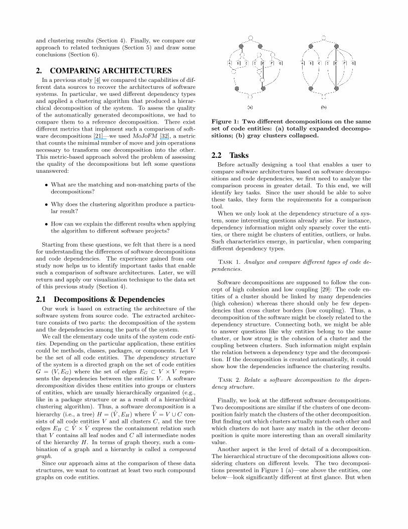
Figure 1: Two different decompositions on the sameset of code entities: (a) totally expanded decompo-sitions; (b) gray clusters collapsed.

2.2 TasksBefore actually designing a tool that enables a user to

compare software architectures based on software decompo-sitions and code dependencies, we first need to analyze thecomparison process in greater detail. To this end, we willidentify key tasks. Since the user should be able to solvethese tasks, they form the requirements for a comparisontool.

When we only look at the dependency structure of a sys-tem, some interesting questions already arise. For instance,dependency information might only sparsely cover the enti-ties, or there might be clusters of entities, outliers, or hubs.Such characteristics emerge, in particular, when comparingdifferent dependency types.

Task 1. Analyze and compare different types of code de-pendencies.

Software decompositions are supposed to follow the con-cept of high cohesion and low coupling [29]: The code en-tities of a cluster should be linked by many dependencies(high cohesion) whereas there should only be few depen-dencies that cross cluster borders (low coupling). Thus, adecomposition of the software might be closely related to thedependency structure. Connecting both, we might be ableto answer questions like why entities belong to the samecluster, or how strong is the cohesion of a cluster and thecoupling between clusters. Such information might explainthe relation between a dependency type and the decomposi-tion. If the decomposition is created automatically, it couldshow how the dependencies influence the clustering results.

Task 2. Relate a software decomposition to the depen-dency structure.

Finally, we look at the different software decompositions.Two decompositions are similar if the clusters of one decom-position fairly match the clusters of the other decomposition.But finding out which clusters actually match each other andwhich clusters do not have any match in the other decom-position is quite more interesting than an overall similarityvalue.

Another aspect is the level of detail of a decomposition.The hierarchical structure of the decompositions allows con-sidering clusters on different levels. The two decomposi-tions presented in Figure 1 (a)—one above the entities, onebelow—look significantly different at first glance. But when

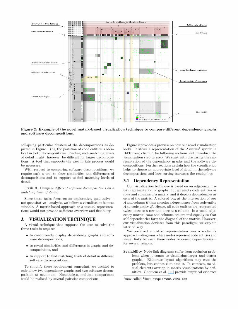
Figure 2: Example of the novel matrix-based visualization technique to compare different dependency graphsand software decompositions.

collapsing particular clusters of the decompositions as de-picted in Figure 1 (b), the partition of code entities is iden-tical in both decompositions. Finding such matching levelsof detail might, however, be difficult for larger decomposi-tions. A tool that supports the user in this process wouldbe necessary.

With respect to comparing software decompositions, werequire such a tool to show similarities and differences ofdecompositions and to support to find matching levels ofdetail.

Task 3. Compare different software decompositions on amatching level of detail.

Since these tasks focus on an explorative, qualitative—not quantitative—analysis, we believe a visualization is mostsuitable. A metric-based approach or a textual representa-tions would not provide sufficient overview and flexibility.

3. VISUALIZATION TECHNIQUEA visual technique that supports the user to solve the

three tasks is required

• to concurrently display dependency graphs and soft-ware decompositions,

• to reveal similarities and differences in graphs and de-compositions, and

• to support to find matching levels of detail in differentsoftware decompositions.

To simplify these requirement somewhat, we decided toonly allow two dependency graphs and two software decom-position at maximum. Nonetheless, multiple comparisonscould be realized by several pairwise comparisons.

Figure 2 provides a preview on how our novel visualizationlooks. It shows a representation of the Azureus1 system, aBitTorrent client. The following sections will introduce thevisualization step by step. We start with discussing the rep-resentation of the dependency graphs and the software de-compositions. Further sections explain how the visualizationhelps to choose an appropriate level of detail in the softwaredecompositions and how sorting increases the readability.

3.1 Dependency RepresentationOur visualization technique is based on an adjacency ma-

trix representation of graphs: It represents code entities asrows and columns of a matrix, and it depicts dependencies ascells of the matrix. A colored box at the intersection of rowA and column B thus encodes a dependency from code entityA to code entity B. Hence, all code entities are representedtwice, once as a row and once as a column. In a usual adja-cency matrix, rows and columns are ordered equally so thatself-dependencies form the diagonal of the matrix. However,our visualization deviates from this paradigm; we explainlater on why.

We preferred a matrix representation over a node-linkapproach—diagrams where nodes represent code entities andvisual links between these nodes represent dependencies—for several reasons:

Scalability Node-link diagrams suffer from occlusion prob-lems when it comes to visualizing larger and densergraphs. Elaborate layout algorithms may ease theproblem, but cannot eliminate it. In contrast, no vi-sual elements overlap in matrix visualizations by defi-nition. Ghoniem et al. [11] provide empirical evidence

1now called Vuze; http://www.vuze.com

for the superiority of matrix representations of largergraphs in many applications.

Edges Since we want to analyze differences in dependencygraphs, we are interested in the existence of particularedges (i.e., dependencies). In contrast, tracking longerpaths—an obvious shortcoming of matrix-based graphvisualizations—is less important for our application.A matrix visualization focuses on edges; it explicitlyshows existing and non-existing edges.

Clusters Depending on a good layout, both node-link andmatrix diagrams are able to reveal clusters. But asHenry et al. [14] point out, for dense clusters, matrixrepresentations still provide detailed information whilenode-link representations produce clutter.

Figure 2 shows that the matrix is the central part of ourvisualization. In this example, we used 477 classes as codeentities. Thus, each cell indicating a dependency has only afew pixels on screen, but we can still see and discern thesesmall points. Moreover, we observe that these colored cellsare not evenly distributed over the image. The visual clus-ters formed by these cells hint at clusters in the dependencystructure.

Our matrix-based approach is able to visualize two graphson the same set of code entities in the same diagram. Thedependencies just need to be drawn in different colors—onecolor for each graph and a third color to represent duplicatedependencies (i.e., dependencies that occur in both graphs).The legend depicts this color scheme. Concurrently visual-izing more than two graphs with this approach is possible,but would probably confuse the user by ambiguous colors.A comparison of n graphs would need 2n−1 different colorsplus a background color.

3.2 Decomposition RepresentationWe consider software decompositions as hierarchies. A

visual representation of a hierarchy can be easily attachedto the sides of the matrix. We use a layered icicle plot [16]to depict a hierarchy. Such an icicle plot lays out the nodessimilar to a usual tree diagram, but depicts each node asa box that fills the available space around the node. It ismore space-efficient and easier to label than an equivalentnode-link hierarchy diagram.

3.2.1 HierarchiesThe visualization in Figure 2 displays a software decom-

position in form of the package structure on the left handside of the diagram. Soft shadows separate the clusters, notonly in the hierarchy but also continuously in the matrix. Ifenough screen space is available, labels identify the clusters.

Since the rows and columns of the matrix can be sortedindependently, we are able to add a second software decom-position on top of the diagram. The example in Figure 2depicts a decomposition automatically generated by a clus-tering algorithm.

The hierarchical structure of each decomposition impliessome constraints on the order of the code entities: Onlysibling entities or clusters are allowed to be switched withoutdestroying the representation of the decomposition. Hence,code entities have to be sorted differently with respect torows than with respect to columns.

3.2.2 Similarity MetricThe task of comparing the two decompositions consists of

finding similarities and differences in the cluster structure.But without assistance, this would be a time-consuming andstrenuous task: Considering a particular cluster, it is hardto identify its most similar correspondent because it has tobe manually compared to every cluster in the other decom-position. A metric that is able to rank the possible corre-spondents with respect of their similarity to a selected nodemight solve the problem.

A cluster consists of a set of code entities. Thus, com-paring two clusters is equivalent to comparing two sets Aand B. To get a similarity measure, we are interested inhow many entities concurrently belong to both clusters inrelation to the size of both clusters. This can be expressedas the size of the intersection of the two sets divided by thesize of the union of the sets—the Jaccard coefficient:

sim(A,B) :=|A ∩B||A ∪B| .

We integrate the similarity information based on the Jac-card coefficients in the background of the matrix representa-tion. The clusters form a matrix-like meta-structure wherethe cluster—not the code entities—represent the rows andcolumns. Each comparison of two clusters can be repre-sented as a cell of this matrix. We use the backgroundbrightness of the cells to encode the Jaccard similarity valueof the according cluster: Dark backgrounds visualize highsimilarity values. Coloring each possible pair of clusters likethis would, however, lead to overlapping cells and thus am-biguous shadings. Hence, this approach is able to comparetwo decompositions only on one level of clusters for each de-composition. In our visualization the user is able to choosethis level manually or supported by an optimization algo-rithm (details will follow in Section 3.3).

Figure 2 shows that the visualization enables the user toidentify similar clusters at a glance: We can immediatelydetect the most similar cluster combinations with the help ofthis background structure. Moreover, non-matched clustersresult in rows or columns consisting only of a set of light-grayboxes without any darker one. Table 1 lists some examplesof such matched and non-matched clusters.

Table 1: Examples of matched and non-matchedclusters in Figure 2.

Package Decomposition Clustered Decomposition

disk 0.0.0tracker.pr.u 0.1.2.6.24

ipfil 0.1.3.3

util.# –– 0.1.1

3.3 Level of DetailNevertheless, when comparing two decompositions, it is

necessary to chose an appropriate level of detail. Especiallyclustered decompositions tend to be deep and fine-grainedhierarchies while, for instance, package structures are nor-mally flat and more coarse-grained.The user should be ableto collapse clusters to find an appropriate level. A level isappropriate if the following conditions are true:

Figure 3: The example from Figure 2 without andwith an appropriately chosen level of detail.

Conformance The decompositions match as far as possiblewith respect to a measure of similarity.

Significance The structure of both decompositions is pre-served (i.e., not too many clusters should be collapsed).

It is always possible to reach maximum conformance bytotally collapsing both decompositions. But this obviouslyviolates the condition of significance. Hence, these two con-ditions usually must be traded off against each other.

Figure 3 gives an example of how important the level ofdetail is. While in the default visualization on the left handside the background patterns are much too fine-grained toeasily find differences and similarities in both decomposi-tions, the right hand side image is much more readable be-cause it has an appropriately chosen level of detail.

3.4 InteractionThe visualization allows the user to collapse or expand

clusters by clicking on their visual representations. Further-more, slim markers on the side of the hierarchy enable theuser to collapse or expand whole hierarchy levels (Figure 2,top left). These markers also indicate which levels are totallycollapsed (light gray), partially collapsed (gray), or fully ex-panded (dark gray). A collapsed cluster still claims as muchspace as an expanded cluster. The main difference is thatcollapsing a cluster moves the cluster comparison to a higherlevel: Larger gray scale background boxes now display thecluster similarity metric values on this higher level.

The gray scale matrix in the background is the most im-portant criterion to assess the similarity of the two decom-positions at a particular level. Roughly speaking, few blackboxes and many white boxes indicate a high conformancewhile many low-contrast gray boxes indicate a low confor-mance. The interactive expand and collapse mechanism al-lows the user to explore different levels, but especially forlarger data sets, a good automatically proposed level of de-tail would be of great help.

3.5 Optimization CriterionTo implement an automatic algorithm, we had to find a

formal optimization criterion that assesses the quality of aparticular level of detail state. Such a state consists of thepartially collapsed decompositions. Each collapsed decom-position implies a partition of the code entities like presentedin the example of Figure 1. Hence, an optimization criterionis a real-valued objective function defined on two partitions.

We propose an objective function that counts the numberof matching clusters of the two partitions P1 and P2. Thedegree of similarity could be again computed by the Jaccard

similarity coefficient. Adding these similarity coefficients forall possible cluster combinations, we come up with the fol-lowing objective function.

f(P1, P2) =∑A∈P1

∑B∈P2

ωA,B ∗ sim(A,B)

To consider the different sizes of the cluster, we added aweighting coefficient ω. For two clusters A and B, the coeffi-cient just sums up the number of elements of both clusters:ωA,B := |A| + |B|. It is independent of the similarity ofthe clusters and gives larger cluster combinations a higherweight.

3.5.1 Significance Level ThresholdsThis objective function, however, only evaluates the level

of detail with respect to conformance and does not considersignificance. But it is difficult to balance significance andconformance in a single objective function. An appropriatebalance might also depend on the concrete application theuser has in mind.

To allow high conformance on different levels of signifi-cance, we introduce a significance level threshold for each ofthe two decompositions. This threshold prevents collapsingclusters beyond this level while optimizing the conformance.

The grid pattern in the upper left corner of the visualiza-tion displays the two significance level thresholds. The useris able to set both levels with a single click. For instance,in Figure 2 the user has clicked on the cell at the intersec-tion of the third column and the third row, indicated by ablack box. This means that both decompositions have tostay expanded up to the third level while optimizing theconformance of the decompositions.

3.5.2 Optimization AlgorithmThe two decompositions, the objective function, and the

two significance level thresholds form a constrained max-imization problem. As an optimization strategy for thisproblem, an exhaustive search, however, is not applicablefor nontrivial data sets. The number of possible partitionsinduced by a single hierarchy might already grow exponen-tially with the number of leaf nodes n: In the worst case—abinary hierarchy—at least the n

2intermediate nodes of the

lowest level can be independently collapsed and expanded.This leads to at least 2

n2 different partitions.

Instead, we use a hill climbing algorithm to find a localmaximum of the optimization problem. As an initializa-tion, the algorithm expands the two decompositions to theminimal level, which is defined by the two significance levelthresholds. Then it tries to maximize the objective func-tion as follows (expand operations that improve the objec-tive function persist while all other expand operations aredirectly undone):

1. Expand each collapsed node of the first hierarchy oneby one.

2. Repeat step (a) for all collapsed nodes of the secondhierarchy.

3. If nothing has improved in step 1 and 2, try to expandtwo nodes concurrently, one in the first and one inthe second hierarchy (systematically over all possiblecombinations).

These three steps are repeated until they cannot provideany further improvement. The third step turned out to behelpful to skip local maxima.

Thus, our optimization strategy provides an interactivelyselectable level of detail with an adaptive refinement to un-derline matching parts of the two decompositions. Clickingon a cell of the threshold visualization, the algorithm auto-matically produces a layout of few black boxes surroundedby many white ones. Figure 3 illustrates this process: Whilethe image on the left hand side shows two totally collapsedhierarchies, the image on the right hand side is actually cre-ated applying the optimization algorithm (this image is alsodepicted in Figure 2 in larger size). In our experiences usingthe visualization, the level of detail optimization turned outto be very valuable because it drastically reduces the timeto find an appropriate level of detail.

3.6 SortingThe linear ordering of the rows and columns is elementary

for the readability of a matrix graph visualization [22]. Witha random ordering no structure would be visible, whereasa good ordering would reveal important graph structureslike clusters, hub vertices, or outliers. Different approachesand algorithms exist to create a reasonable layout—Muelleret al. [22] as well as Henry and Fekete [13] survey thesetechniques in detail.

The hierarchical representation of the two software de-compositions, however, constrains this ordering in our visu-alization. If the decomposition follows a certain semantic,this mandatory sorting may already help to reveal the struc-ture of the dependency graphs. Nevertheless, the orderingstill leaves some degree of freedom: The positions of siblingclusters and code entities can be switched.

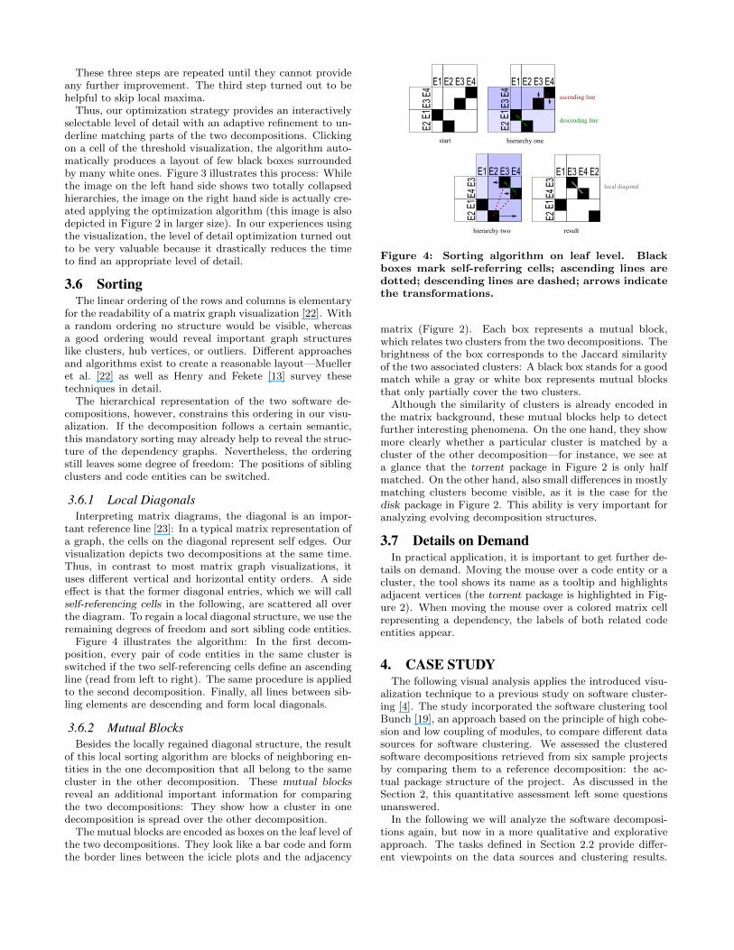
3.6.1 Local DiagonalsInterpreting matrix diagrams, the diagonal is an impor-

tant reference line [23]: In a typical matrix representation ofa graph, the cells on the diagonal represent self edges. Ourvisualization depicts two decompositions at the same time.Thus, in contrast to most matrix graph visualizations, ituses different vertical and horizontal entity orders. A sideeffect is that the former diagonal entries, which we will callself-referencing cells in the following, are scattered all overthe diagram. To regain a local diagonal structure, we use theremaining degrees of freedom and sort sibling code entities.

Figure 4 illustrates the algorithm: In the first decom-position, every pair of code entities in the same cluster isswitched if the two self-referencing cells define an ascendingline (read from left to right). The same procedure is appliedto the second decomposition. Finally, all lines between sib-ling elements are descending and form local diagonals.

3.6.2 Mutual BlocksBesides the locally regained diagonal structure, the result

of this local sorting algorithm are blocks of neighboring en-tities in the one decomposition that all belong to the samecluster in the other decomposition. These mutual blocksreveal an additional important information for comparingthe two decompositions: They show how a cluster in onedecomposition is spread over the other decomposition.

The mutual blocks are encoded as boxes on the leaf level ofthe two decompositions. They look like a bar code and formthe border lines between the icicle plots and the adjacency

Figure 4: Sorting algorithm on leaf level. Blackboxes mark self-referring cells; ascending lines aredotted; descending lines are dashed; arrows indicatethe transformations.

matrix (Figure 2). Each box represents a mutual block,which relates two clusters from the two decompositions. Thebrightness of the box corresponds to the Jaccard similarityof the two associated clusters: A black box stands for a goodmatch while a gray or white box represents mutual blocksthat only partially cover the two clusters.

Although the similarity of clusters is already encoded inthe matrix background, these mutual blocks help to detectfurther interesting phenomena. On the one hand, they showmore clearly whether a particular cluster is matched by acluster of the other decomposition—for instance, we see ata glance that the torrent package in Figure 2 is only halfmatched. On the other hand, also small differences in mostlymatching clusters become visible, as it is the case for thedisk package in Figure 2. This ability is very important foranalyzing evolving decomposition structures.

3.7 Details on DemandIn practical application, it is important to get further de-

tails on demand. Moving the mouse over a code entity or acluster, the tool shows its name as a tooltip and highlightsadjacent vertices (the torrent package is highlighted in Fig-ure 2). When moving the mouse over a colored matrix cellrepresenting a dependency, the labels of both related codeentities appear.

4. CASE STUDYThe following visual analysis applies the introduced visu-

alization technique to a previous study on software cluster-ing [4]. The study incorporated the software clustering toolBunch [19], an approach based on the principle of high cohe-sion and low coupling of modules, to compare different datasources for software clustering. We assessed the clusteredsoftware decompositions retrieved from six sample projectsby comparing them to a reference decomposition: the ac-tual package structure of the project. As discussed in theSection 2, this quantitative assessment left some questionsunanswered.

In the following we will analyze the software decomposi-tions again, but now in a more qualitative and explorativeapproach. The tasks defined in Section 2.2 provide differ-ent viewpoints on the data sources and clustering results.

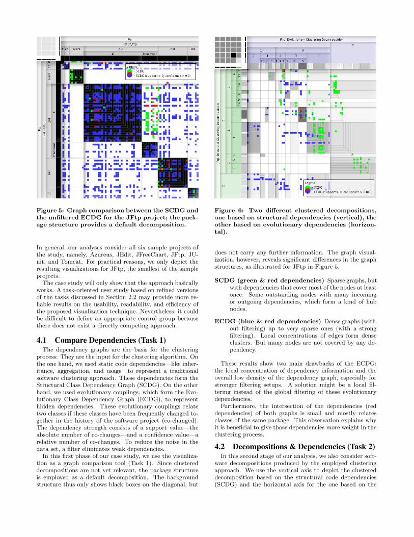
Figure 5: Graph comparison between the SCDG andthe unfiltered ECDG for the JFtp project; the pack-age structure provides a default decomposition.

In general, our analyses consider all six sample projects ofthe study, namely, Azureus, JEdit, JFreeChart, JFtp, JU-nit, and Tomcat. For practical reasons, we only depict theresulting visualizations for JFtp, the smallest of the sampleprojects.

The case study will only show that the approach basicallyworks. A task-oriented user study based on refined versionsof the tasks discussed in Section 2.2 may provide more re-liable results on the usability, readability, and efficiency ofthe proposed visualization technique. Nevertheless, it couldbe difficult to define an appropriate control group becausethere does not exist a directly competing approach.

4.1 Compare Dependencies (Task 1)The dependency graphs are the basis for the clustering

process: They are the input for the clustering algorithm. Onthe one hand, we used static code dependencies—like inher-itance, aggregation, and usage—to represent a traditionalsoftware clustering approach. These dependencies form theStructural Class Dependency Graph (SCDG). On the otherhand, we used evolutionary couplings, which form the Evo-lutionary Class Dependency Graph (ECDG), to representhidden dependencies. These evolutionary couplings relatetwo classes if these classes have been frequently changed to-gether in the history of the software project (co-changed).The dependency strength consists of a support value—theabsolute number of co-changes—and a confidence value—arelative number of co-changes. To reduce the noise in thedata set, a filter eliminates weak dependencies.

In this first phase of our case study, we use the visualiza-tion as a graph comparison tool (Task 1). Since clustereddecompositions are not yet relevant, the package structureis employed as a default decomposition. The backgroundstructure thus only shows black boxes on the diagonal, but

Figure 6: Two different clustered decompositions,one based on structural dependencies (vertical), theother based on evolutionary dependencies (horizon-tal).

does not carry any further information. The graph visual-ization, however, reveals significant differences in the graphstructures, as illustrated for JFtp in Figure 5.

SCDG (green & red dependencies) Sparse graphs, butwith dependencies that cover most of the nodes at leastonce. Some outstanding nodes with many incomingor outgoing dependencies, which form a kind of hubnodes.

ECDG (blue & red dependencies) Dense graphs (with-out filtering) up to very sparse ones (with a strongfiltering). Local concentrations of edges form denseclusters. But many nodes are not covered by any de-pendency.

These results show two main drawbacks of the ECDG:the local concentration of dependency information and theoverall low density of the dependency graph, especially forstronger filtering setups. A solution might be a local fil-tering instead of the global filtering of these evolutionarydependencies.

Furthermore, the intersection of the dependencies (reddependencies) of both graphs is small and mostly relatesclasses of the same package. This observation explains whyit is beneficial to give those dependencies more weight in theclustering process.

4.2 Decompositions & Dependencies (Task 2)In this second stage of our analysis, we also consider soft-

ware decompositions produced by the employed clusteringapproach. We use the vertical axis to depict the clustereddecomposition based on the structural code dependencies(SCDG) and the horizontal axis for the one based on the

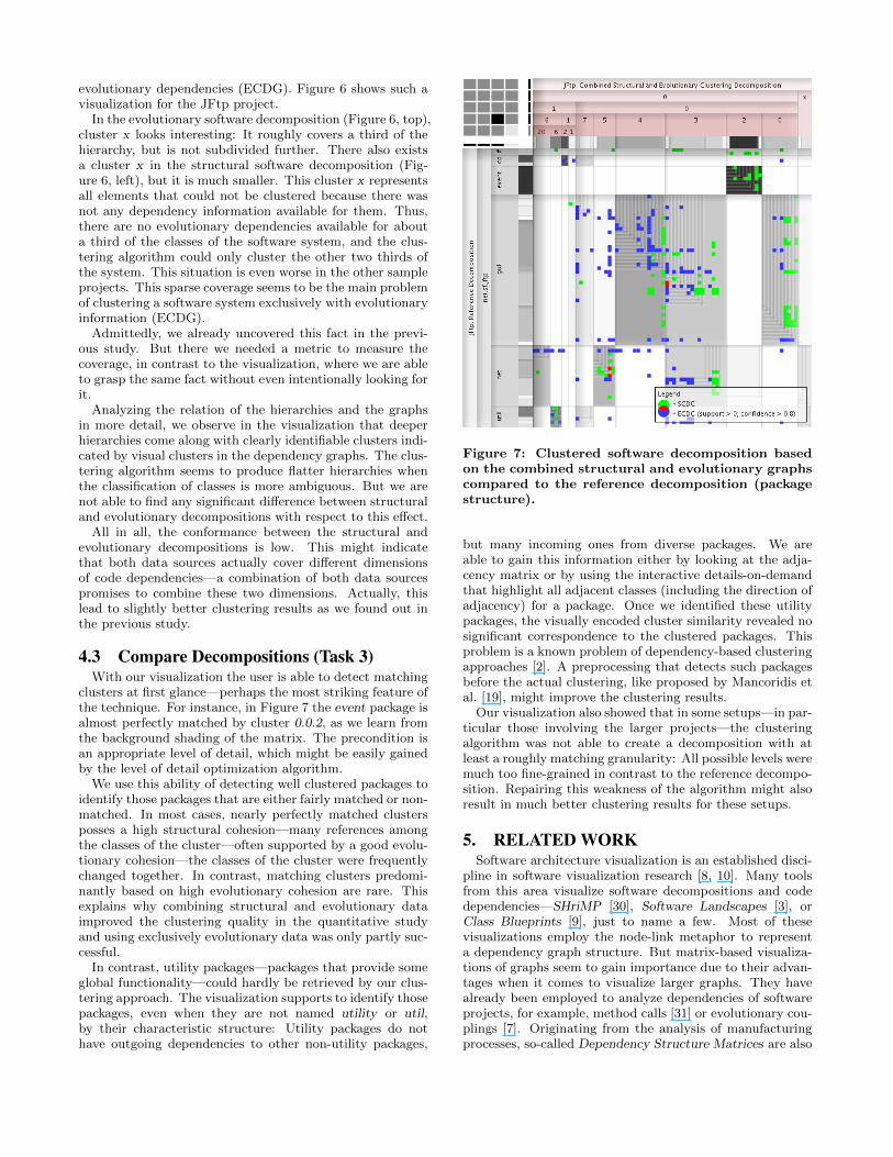
evolutionary dependencies (ECDG). Figure 6 shows such avisualization for the JFtp project.

In the evolutionary software decomposition (Figure 6, top),cluster x looks interesting: It roughly covers a third of thehierarchy, but is not subdivided further. There also existsa cluster x in the structural software decomposition (Fig-ure 6, left), but it is much smaller. This cluster x representsall elements that could not be clustered because there wasnot any dependency information available for them. Thus,there are no evolutionary dependencies available for abouta third of the classes of the software system, and the clus-tering algorithm could only cluster the other two thirds ofthe system. This situation is even worse in the other sampleprojects. This sparse coverage seems to be the main problemof clustering a software system exclusively with evolutionaryinformation (ECDG).

Admittedly, we already uncovered this fact in the previ-ous study. But there we needed a metric to measure thecoverage, in contrast to the visualization, where we are ableto grasp the same fact without even intentionally looking forit.

Analyzing the relation of the hierarchies and the graphsin more detail, we observe in the visualization that deeperhierarchies come along with clearly identifiable clusters indi-cated by visual clusters in the dependency graphs. The clus-tering algorithm seems to produce flatter hierarchies whenthe classification of classes is more ambiguous. But we arenot able to find any significant difference between structuraland evolutionary decompositions with respect to this effect.

All in all, the conformance between the structural andevolutionary decompositions is low. This might indicatethat both data sources actually cover different dimensionsof code dependencies—a combination of both data sourcespromises to combine these two dimensions. Actually, thislead to slightly better clustering results as we found out inthe previous study.

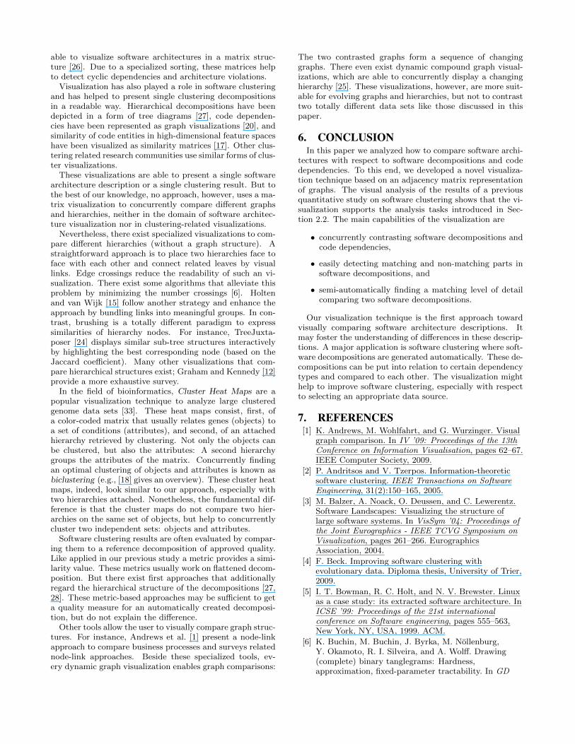
4.3 Compare Decompositions (Task 3)With our visualization the user is able to detect matching

clusters at first glance—perhaps the most striking feature ofthe technique. For instance, in Figure 7 the event package isalmost perfectly matched by cluster 0.0.2, as we learn fromthe background shading of the matrix. The precondition isan appropriate level of detail, which might be easily gainedby the level of detail optimization algorithm.

We use this ability of detecting well clustered packages toidentify those packages that are either fairly matched or non-matched. In most cases, nearly perfectly matched clustersposses a high structural cohesion—many references amongthe classes of the cluster—often supported by a good evolu-tionary cohesion—the classes of the cluster were frequentlychanged together. In contrast, matching clusters predomi-nantly based on high evolutionary cohesion are rare. Thisexplains why combining structural and evolutionary dataimproved the clustering quality in the quantitative studyand using exclusively evolutionary data was only partly suc-cessful.

In contrast, utility packages—packages that provide someglobal functionality—could hardly be retrieved by our clus-tering approach. The visualization supports to identify thosepackages, even when they are not named utility or util,by their characteristic structure: Utility packages do nothave outgoing dependencies to other non-utility packages,

Figure 7: Clustered software decomposition basedon the combined structural and evolutionary graphscompared to the reference decomposition (packagestructure).

but many incoming ones from diverse packages. We areable to gain this information either by looking at the adja-cency matrix or by using the interactive details-on-demandthat highlight all adjacent classes (including the direction ofadjacency) for a package. Once we identified these utilitypackages, the visually encoded cluster similarity revealed nosignificant correspondence to the clustered packages. Thisproblem is a known problem of dependency-based clusteringapproaches [2]. A preprocessing that detects such packagesbefore the actual clustering, like proposed by Mancoridis etal. [19], might improve the clustering results.

Our visualization also showed that in some setups—in par-ticular those involving the larger projects—the clusteringalgorithm was not able to create a decomposition with atleast a roughly matching granularity: All possible levels weremuch too fine-grained in contrast to the reference decompo-sition. Repairing this weakness of the algorithm might alsoresult in much better clustering results for these setups.

5. RELATED WORKSoftware architecture visualization is an established disci-

pline in software visualization research [8, 10]. Many toolsfrom this area visualize software decompositions and codedependencies—SHriMP [30], Software Landscapes [3], orClass Blueprints [9], just to name a few. Most of thesevisualizations employ the node-link metaphor to representa dependency graph structure. But matrix-based visualiza-tions of graphs seem to gain importance due to their advan-tages when it comes to visualize larger graphs. They havealready been employed to analyze dependencies of softwareprojects, for example, method calls [31] or evolutionary cou-plings [7]. Originating from the analysis of manufacturingprocesses, so-called Dependency Structure Matrices are also

able to visualize software architectures in a matrix struc-ture [26]. Due to a specialized sorting, these matrices helpto detect cyclic dependencies and architecture violations.

Visualization has also played a role in software clusteringand has helped to present single clustering decompositionsin a readable way. Hierarchical decompositions have beendepicted in a form of tree diagrams [27], code dependen-cies have been represented as graph visualizations [20], andsimilarity of code entities in high-dimensional feature spaceshave been visualized as similarity matrices [17]. Other clus-tering related research communities use similar forms of clus-ter visualizations.

These visualizations are able to present a single softwarearchitecture description or a single clustering result. But tothe best of our knowledge, no approach, however, uses a ma-trix visualization to concurrently compare different graphsand hierarchies, neither in the domain of software architec-ture visualization nor in clustering-related visualizations.

Nevertheless, there exist specialized visualizations to com-pare different hierarchies (without a graph structure). Astraightforward approach is to place two hierarchies face toface with each other and connect related leaves by visuallinks. Edge crossings reduce the readability of such an vi-sualization. There exist some algorithms that alleviate thisproblem by minimizing the number crossings [6]. Holtenand van Wijk [15] follow another strategy and enhance theapproach by bundling links into meaningful groups. In con-trast, brushing is a totally different paradigm to expresssimilarities of hierarchy nodes. For instance, TreeJuxta-poser [24] displays similar sub-tree structures interactivelyby highlighting the best corresponding node (based on theJaccard coefficient). Many other visualizations that com-pare hierarchical structures exist; Graham and Kennedy [12]provide a more exhaustive survey.

In the field of bioinformatics, Cluster Heat Maps are apopular visualization technique to analyze large clusteredgenome data sets [33]. These heat maps consist, first, ofa color-coded matrix that usually relates genes (objects) toa set of conditions (attributes), and second, of an attachedhierarchy retrieved by clustering. Not only the objects canbe clustered, but also the attributes: A second hierarchygroups the attributes of the matrix. Concurrently findingan optimal clustering of objects and attributes is known asbiclustering (e.g., [18] gives an overview). These cluster heatmaps, indeed, look similar to our approach, especially withtwo hierarchies attached. Nonetheless, the fundamental dif-ference is that the cluster maps do not compare two hier-archies on the same set of objects, but help to concurrentlycluster two independent sets: objects and attributes.

Software clustering results are often evaluated by compar-ing them to a reference decomposition of approved quality.Like applied in our previous study a metric provides a simi-larity value. These metrics usually work on flattened decom-position. But there exist first approaches that additionallyregard the hierarchical structure of the decompositions [27,28]. These metric-based approaches may be sufficient to geta quality measure for an automatically created decomposi-tion, but do not explain the difference.

Other tools allow the user to visually compare graph struc-tures. For instance, Andrews et al. [1] present a node-linkapproach to compare business processes and surveys relatednode-link approaches. Beside these specialized tools, ev-ery dynamic graph visualization enables graph comparisons:

The two contrasted graphs form a sequence of changinggraphs. There even exist dynamic compound graph visual-izations, which are able to concurrently display a changinghierarchy [25]. These visualizations, however, are more suit-able for evolving graphs and hierarchies, but not to contrasttwo totally different data sets like those discussed in thispaper.

6. CONCLUSIONIn this paper we analyzed how to compare software archi-

tectures with respect to software decompositions and codedependencies. To this end, we developed a novel visualiza-tion technique based on an adjacency matrix representationof graphs. The visual analysis of the results of a previousquantitative study on software clustering shows that the vi-sualization supports the analysis tasks introduced in Sec-tion 2.2. The main capabilities of the visualization are

• concurrently contrasting software decompositions andcode dependencies,

• easily detecting matching and non-matching parts insoftware decompositions, and

• semi-automatically finding a matching level of detailcomparing two software decompositions.

Our visualization technique is the first approach towardvisually comparing software architecture descriptions. Itmay foster the understanding of differences in these descrip-tions. A major application is software clustering where soft-ware decompositions are generated automatically. These de-compositions can be put into relation to certain dependencytypes and compared to each other. The visualization mighthelp to improve software clustering, especially with respectto selecting an appropriate data source.

7. REFERENCES[1] K. Andrews, M. Wohlfahrt, and G. Wurzinger. Visual

graph comparison. In IV ’09: Proceedings of the 13thConference on Information Visualisation, pages 62–67.IEEE Computer Society, 2009.

[2] P. Andritsos and V. Tzerpos. Information-theoreticsoftware clustering. IEEE Transactions on SoftwareEngineering, 31(2):150–165, 2005.

[3] M. Balzer, A. Noack, O. Deussen, and C. Lewerentz.Software Landscapes: Visualizing the structure oflarge software systems. In VisSym ’04: Proceedings ofthe Joint Eurographics - IEEE TCVG Symposium onVisualization, pages 261–266. EurographicsAssociation, 2004.

[4] F. Beck. Improving software clustering withevolutionary data. Diploma thesis, University of Trier,2009.

[5] I. T. Bowman, R. C. Holt, and N. V. Brewster. Linuxas a case study: its extracted software architecture. InICSE ’99: Proceedings of the 21st internationalconference on Software engineering, pages 555–563,New York, NY, USA, 1999. ACM.

[6] K. Buchin, M. Buchin, J. Byrka, M. Nollenburg,Y. Okamoto, R. I. Silveira, and A. Wolff. Drawing(complete) binary tanglegrams: Hardness,approximation, fixed-parameter tractability. In GD

’08: 16th International Symposium on Graph Drawing,Lecture Notes in Computer Science, pages 324–335.Springer, 2008.

[7] M. Burch, S. Diehl, and P. Weißgerber. Visual datamining in software archives. In SoftVis ’05:Proceedings of the 2005 ACM Symposium on SoftwareVisualization, pages 37–46, New York, NY, USA,2005. ACM Press.

[8] S. Diehl. Software Visualization: Visualizing theStructure, Behaviour, and Evolution of Software.Springer, May 2007.

[9] S. Ducasse and M. Lanza. The class blueprint:Visually supporting the understanding of classes.IEEE Transactions on Software Engineering,31(1):75–90, 2005.

[10] Y. Ghanam and S. Carpendale. A survey paper onsoftware architecture visualization. Technical report,2008.

[11] M. Ghoniem, J. D. Fekete, and P. Castagliola. Acomparison of the readability of graphs usingnode-link and matrix-based representations. InINFOVIS ’04: IEEE Symposium on InformationVisualization, pages 17–24, 2004.

[12] M. Graham and J. Kennedy. A survey of multiple treevisualisation. Information Visualization, 2009.

[13] N. Henry and J.-D. Fekete. Matrixexplorer: adual-representation system to explore social networks.IEEE Transactions on Visualization and ComputerGraphics, 12(5):677–684, September 2006.

[14] N. Henry, J. D. Fekete, and M. J. Mcguffin. Nodetrix:a hybrid visualization of social networks. IEEETransactions on Visualization and ComputerGraphics, 13(6):1302–1309, 2007.

[15] D. Holten and J. J. van Wijk. Visual comparison ofhierarchically organized data. Computer GraphicsForum, 27(3):759–766, 2008.

[16] J. B. Kruskal and J. M. Landwehr. Icicle plots: Betterdisplays for hierarchical clustering. The AmericanStatistician, 37(2):162–168, 1983.

[17] A. Kuhn, S. Ducasse, and T. Gırba. Enriching reverseengineering with semantic clustering. In WCRE ’05:Proceedings of the 12th Working Conference onReverse Engineering, pages 133–142, Washington, DC,USA, 2005. IEEE Computer Society.

[18] S. C. Madeira and A. L. Oliveira. Biclusteringalgorithms for biological data analysis: A survey.IEEE/ACM Transactions on Computational Biologyand Bioinformatics, 1(1):24–45, 2004.

[19] S. Mancoridis, B. S. Mitchell, Y. Chen, and E. R.Gansner. Bunch: A clustering tool for the recoveryand maintenance of software system structures. InICSM ’99: Proceedings of the IEEE InternationalConference on Software Maintenance, pages 50–59,Washington, DC, USA, 1999. IEEE Computer Society.

[20] S. Mancoridis, B. S. Mitchell, C. Rorres, Y. Chen, andE. R. Gansner. Using automatic clustering to producehigh-level system organizations of source code. InIWPC ’98: Proceedings of the 6th InternationalWorkshop on Program Comprehension, pages 45–52,Washington, DC, USA, 1998. IEEE Computer Society.

[21] O. Maqbool and H. A. Babri. Hierarchical clustering

for software architecture recovery. IEEE Transactionson Software Engineering, 33(11):759–780, 2007.

[22] C. Mueller, B. Martin, and A. Lumsdaine. Acomparison of vertex ordering algorithms for largegraph visualization. In APVIS ’07: Proceedings of the6th International Asia-Pacific Symposium onVisualization, pages 141–148, 2007.

[23] C. Mueller, B. Martin, and A. Lumsdaine.Interpreting large visual similarity matrices. In APVIS’07: Proceedings of the 6th International Asia-PacificSymposium on Visualization, pages 149–152, 2007.

[24] T. Munzner, F. Guimbretiere, S. Tasiran, L. Zhang,and Y. Zhou. Treejuxtaposer: scalable tree comparisonusing focus+context with guaranteed visibility. ACMTransactions on Graphics, 22(3):453–462, July 2003.

[25] M. Pohl and P. Birke. Interactive exploration of largedynamic networks. In VISUAL ’08: Proceedings of the10th international conference on Visual InformationSystems, pages 56–67, Berlin, Heidelberg, 2008.Springer-Verlag.

[26] N. Sangal, E. Jordan, V. Sinha, and D. Jackson. Usingdependency models to manage complex softwarearchitecture. In OOPSLA ’05: Proceedings of the 20thannual ACM SIGPLAN conference on Object-orientedprogramming, systems, languages, and applications,volume 40, pages 167–176, New York, NY, USA,October 2005. ACM.

[27] M. Shtern and V. Tzerpos. A framework for thecomparison of nested software decompositions. InWCRE ’04: Proceedings of the 11th WorkingConference on Reverse Engineering, pages 284–292,Washington, DC, USA, 2004. IEEE Computer Society.

[28] M. Shtern and V. Tzerpos. Lossless comparison ofnested software decompositions. In WCRE ’07:Proceedings of the 14th Working Conference onReverse Engineering, pages 249–258, Washington, DC,USA, 2007. IEEE Computer Society.

[29] W. P. Stevens, G. J. Myers, and L. L. Constantine.Structured design. IBM Systems Journal,13(2):115–139, 1974.

[30] M. A. Storey, C. Best, and J. Michaud. SHriMPviews: An interactive environment for exploring javaprograms. International Conference on ProgramComprehension, 0, 2001.

[31] F. van Ham. Using multilevel call matrices in largesoftware projects. In INFOVIS ’03: Proceedings of theIEEE Symposium on Information Visualization, pages227–232, 2003.

[32] Z. Wen and V. Tzerpos. An effectiveness measure forsoftware clustering algorithms. In IWPC ’04:Proceedings of the 12th International Workshop onProgram Comprehension, pages 194–203. IEEEComputer Society, 2004.

[33] L. Wilkinson and M. Friendly. The history of thecluster heat map. The American Statistician,63(2):179–184, 2009.

[34] T. Zimmermann, S. Diehl, and A. Zeller. How historyjustifies system architecture (or not). In IWPSE ’03:Proceedings of the 6th International Workshop onPrinciples of Software Evolution, Washington, DC,USA, 2003. IEEE Computer Society.