NORTII-HOLLAND

A Comparison of Methods for Representing Topological Relationships

ELISEO CLEMENTINI

and

PAOLINO DI FELICE

Department of Electrical Engineerzng, Universzty of L 'Aquzla, 67040 Poggio di Roio, L 'Aquila, Italy

ABSTRACT

In the field of spatial information systems, a primary need is to develop a sound theory of topological relationships between spatial objects. A category of formal methods for representing topological relationships is based on point-set theory. In this paper, a high level calculus-based method is compared with such point­set methods. It is shown that the calculus-based method is able to distinguish among finer topological configurations than most of the point-set methods. The advantages of the calculus-based method are the direct use in a calculus-based spatial query language and the capability of representing topological relationships among a significant set of spatial objects by means of only five relationship names and two boundary operators.

l. INTRODUCTION

Topological properties of spatial objects commonly used in Geographical Information Systems (GIS) are the primary information which users of such systems need to deal with (e.g., see [13]). Queries of the type, "Are these two regions bordering on each other?" and "vVhich are the rivers crossing this province?," are surely the most simple and widely addressed to a GIS, while queries involving metric properties and ordering properties represent a deeper step of spatial analysis. The importance of topological properties in a spatial query language is related directly to the learning process adopted by humans with regard to space. Transformations that do not preserve topology are the most radical ones and are difficult to learn [2].

INFORMATION SCIENCES 3,149-178 (1995) © ElseVIer SCience Inc., 1995 655 Avenue of the Amenca.s. New York. :.lY 10010

0020-0255/95/$9.50 SSDI 0020-0255(94)00033-8

150 E. CLEMENTINI AND P. DI FELICE

Early descriptions of topological relationships (e.g., [11]) did not have enough formal basis to support a spatial query language, which needs for­mal definitions in order to specify exact algorithms to assess relationships. The approach usually taken in a broad family of spatial query languages for various applications (e.g., ATLAS [21], .YIAPQUERY [10], KBCIS-II [19], PSQL [17], geo-relational algebra [12], spatial SQL [7], PIC QUERY +[3]) is that the language includes some topological operators among a given set of spatial operators, such as "touch," "adjacent," "within," etc. The problem is that none of the above spatial query languages discusses such issues like the expressive power of the topological operators being proposed or their completeness with respect to a certain depth of topological description.

The importance of defining a sound and complete set of topological re­lationships is recognized in [9, 18]. This allows an algebraic approach for spatial relationships, which supports a correct query processing and the possibility of pointing out exactly which is the category of topological con­figurations that can be recognized by posing spatial queries. A formal approach allows also to extend easily the basic tools in order to accom­modate users who need to distinguish topological configurations among a greater extent of granularity. The other important issue is, Which is the expressive power the users expect in a topological query language and what are the topological relationship names the users need to be available for a particular spatial application? The names for relationships should suit the needs of users in a large variety of cases or at a higher level of abstrac­tion the system should allow to rename spatial operators to fit specific requirements.

In the perspective presented in this paper, we regard the geographic space as a pure topological space without the additional load of a metric. There arc different levels of meaning at which spatial information may be organized. Some literature refers to vector and raster models; others refer to geometric objects, conceptual entities, and so on. Often, the approaches are difficult to understand because they do not state exactly at which level they want to be. A recent clear categorization of levels of meaning for geographic information can be found in [14], where five of them are iden­tified, varying from the bottom one related to physical data structures to the upper one related to real-world phenomena. Our work fits in the so­called "conceptual spatial object level," supporting descriptions of space in terms of the two-dimensional spatial object primitives, the point, the line, and the area, and also in terms of the spatial relationships between such primitives, and in particular topological relationships.

The methods taken into consideration herein are those based on point­set topology [8, 9, 16] and the one based on a formal calculus [6]. Both approaches satisfy the requirements that they provide formal definitions for

REPRESENTIKG TOPOLOGICAL RELATIONSHIPS 151

topological relationships and that such relationships are sound and com­plete. The comparison between the calculus-based method (CBM) and the point-set methods leads to be consideration that the CBM is equivalent to a combination of the other methods. in the sense that it is able to describe topological facts at the same level of detail. The advantage of the CBM with respect to the point-set methods is the small number of topological relationships with overloaded semantics that are valid for all three types of spatial object primitives. The CBM uses just five topological relation­ships (plus two boundary operators), against a rather higher number of relationships in the point-set methods.

The other advantage of the CBM is the ease of use also at a higher level of meaning. Even if our level of description is related to geometry, the five relationships can be used directly also at the entity object level [14] since their meaning is reasonably easy to understand for end-users. The CBM spatial primitives can be directly integrated in a formal spatial query language for an object-oriented geographic database, called the object cal­culus [4]. We added the object calculus features to GEO++ [22], which is an experimental GIS based on the Postgres extensible database system [20]. The implementation is described in [5].

In Section 2, we give the model for geographic space used throughout the paper. In Section 3, we recall the 4-intersection method (4IM), while in Section 4, we recall the 9-intersection method (9IM). In Section 5, we discuss briefly the dimension extended method (DEM). Section 6 gives the definitions for the CBM. In Section 7, we compare the CBM method with the latter point-set methods, shmving that they are less expressive than the CBM. Then, we define a new point-set method resulting from a combination of the others, and prove that such a combination is equivalent to the CBM. In addition, the category of topological cases that the CBM is able to recognize is explicitly identified.

2. THE SPATIAL MODEL

Geographic objects are usually represented on a geographic map as two­dimensional geometric features. In the present paper, we concentrate on the geometry of the geographic objects, namely, we see them either as points, lines, or areas, irrespective of their meaning at the user level.

In our investigation, we use the concepts of continuity, closure, interior, and boundary that are defined in terms of the neighborhood relation. This approach to give formal definitions of geometric objects (features) and re­lationships is based on point-set topology since features are sets and points are elements of these sets [15]. The study of topological relationships be­tween objects also depends on the embedding space, that we assume is

152 E. CLEMENTINI AND P. DI FELICE

IR2, since we are interested in relationships between features commonly used in GIS.

A topological space is generally described as a set of arbitrary elements (points) in which a concept of continuity is specified. Let X and Y be topological spaces. A mapping f: X ---+ Y is said to be continuous if for each open subset V of Y, the set f-l(V) is an open subset of X. If a mapping f is a bijection and if both f and the inverse f- 1

: Y ---+ X are continuous, then f is called a topological zsomorphism. Topological isomorphisms preserve the neighborhood relations between mapped points and include translation, rotation, and scaling. Topological relationships are those remaining invariant under a topological isomorphism.

To define topological relationships, the following set of operations is used: boundary (8), interior (0), exterior (-), set intersection (n), and dimension (dim). The latter one is a function, which returns the dimension of a point-set or nil (-) for the empty set. In case the point-set consists of multiple parts, then the highest dimension is returned.

In our investigation, we avoid taking into account all kinds of complex geometric objects since these objects may be later considered as extensions of simple ones. Specifically, we consider "simple" area, line, and point features of IR2, defined as follows:

• area features are the closure of simply connected two-dimensional open point-sets of IR?;

• line features are closed connected one-dimensional point-sets embed­ded in IR2 with no self-intersections and with exactly two end-points;

• point features are zero-dimensional sets consisting of only one element offfi2.

We give an algebraic definition [1] for the boundary, interior, and exterior of each of the three types of features. The letters P, L and A are used to indicate point, line, and area features. If it is necessary to distinguish between two features of the same type, then numbers are used, e.g., Ai and A 2 . The symbol>.. may represent anyone of the three feature types. The boundary of a feature is defined as follows:

• the boundary 8A of an area feature A is a closed curve homeomorphic to a I-sphere;

• the boundary 8L of a line feature L is a set containing the two end­points of L;

• the boundary of a point feature P is empty (8P = 0).

Since every feature>.. is a closed set, >.. is equal to its closure, that is, >.. = :\.

REPRESENTIKG TOPOLOGICAL RELATIONSHIPS 153

The interior A a of a generic feature A may be defined as

AO = A - (JA.

As a consequence, the interior of a point feature P is equal to the feature itself: po = P.

The exterior A - of a feature A is defined as

3. THE 4-INTERSECTION METHOD

In [16]' Pullar and Egenhofer originally described the 4IM for classifying to]'ological relationships between one-dimensional intervals of IRI. In [8], Egenhofer and Franzosa adopted the same method for classifying topolog­ical relationships between area features in m 2 . By considering also point and line features, we can distinguish among six major groups of binary relationships: area/area, line/area, point/area, line/line, point/line, and point/point. In the 4IM, the classification of relationships is based on the intersections of the boundaries and interiors of two features A1, A2. Each intersection may be empty (0) or non empty (-.0), resulting in a total of 24 = 16 combinations. Each case is represented by a matrix of values:

It is possible to apply some simple geometric considerations to assess that not all combinations make sense for simple objects. vVe call these combi­nations the impossible cases. Also, we point out the converse relationships, which correspond to pairs of matrices !vf1 , Nh such that M1 = !vfr

By not considering the impossible cases and considering just one case for each pair of converse relationships, we arrive at the result shown in Table 1, where there are in total 37 distinct and mutually exclusive re­lationships between features. In detail, in the area/area group, as there are 8 impossible cases and 2 pairs of converse relationships, the number of different types of relationships is G. Line/area cases are 11 because there are 5 impossible cases; line/line cases are 12 because there are 4 pairs of converse relationships. The possible cases are only 3 for the point/area and point/line groups and 2 for the point/point group.

154 E. CLEMENTINI AND P. DI FELICE

TABLE 1 A Summary of the 4I:Vr. The Number of Real Cases is Obtained from Possible

Cases by Considering Pairs of Converse Relationships as a Single Case

Relationship Groups

Area/area Line/area Point/area Line/line Point/line Point/point

Relationship Groups

Area/area Line/area Point / area Line/line Point/line Point/point

No. of Possible Cases No. of Real Cases

8 6 11 11 3 3

16 12 :3 3 2 2

Total 37

TABLE 2 A Summary of the 9IM

No. of Possible Cases No. of Real Cases

8 6 19 19

3 3 33 23

:3 3 :2 2

Total 56

4. THE 9-INTERSECTION METHOD

The 9IM is an extension of the 4IM based on also considering the exterior of features, besides interior and boundary [9]. Therefore, it is necessary to consider the following matrix of nine sets:

By considering the empty or nonempty content of such nine sets, the total is 29 = 512 theoretical combinations. Excluding the impossible cases, we have the 68 possible cases shown in Table 2. Considering also the converse relationships, we can exclude another 2 cases for the area/area group and 10 cases for the line/line group, having a total of 56 real cases.

REPRESE:-.ITING TOPOLOGICAL RELATIO~SHIPS 155

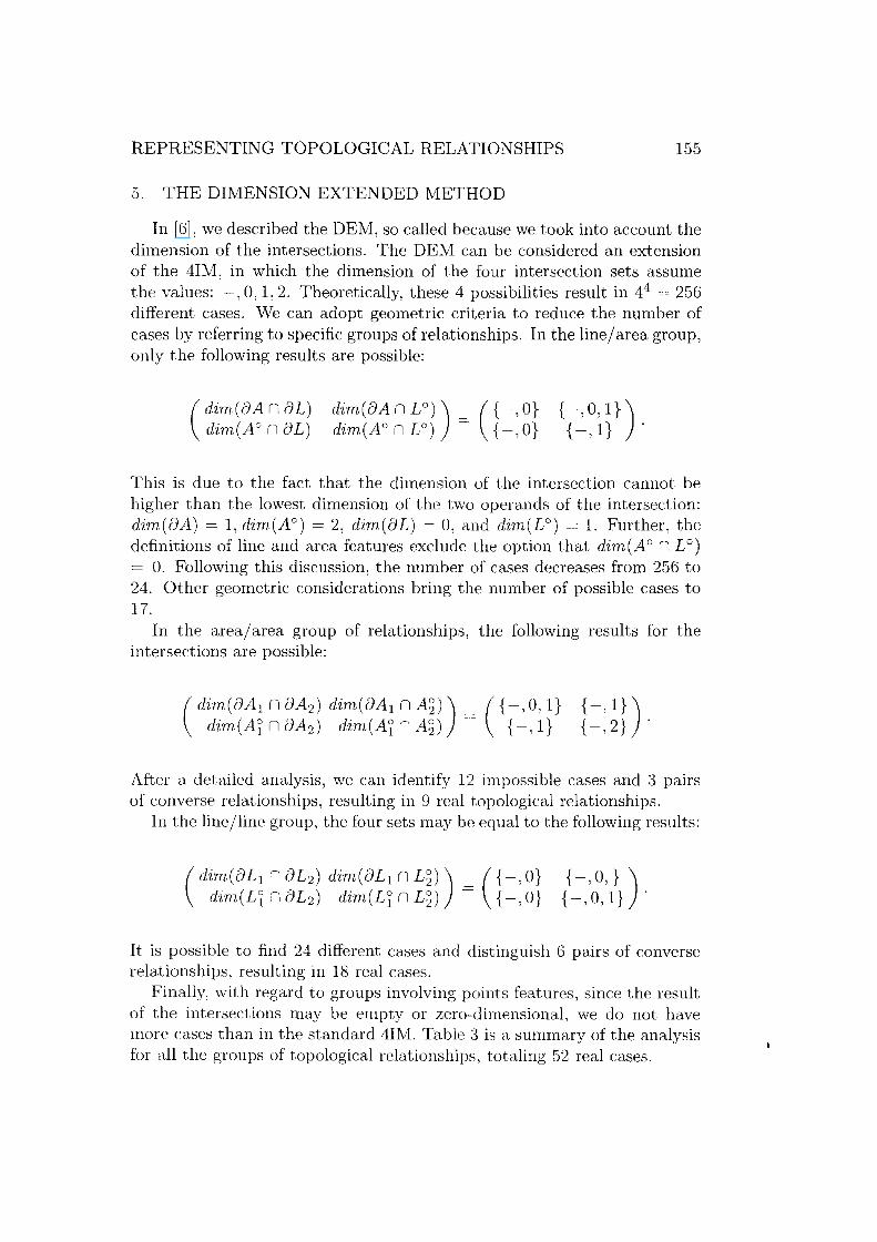
5. THE DIMENSION EXTENDED METHOD

In [6]' we described the DEM, so called because we took into account the dimension of the intersections. The DEM can be considered an extension of the 4I:vi, in which the dimension of the four intersection sets assume the values: ~,O, 1,2. Theoretically, these 4 possibilities result in 44 = 256 different cases. We can adopt geometric criteria to reduce the number of cases by referring to specific groups of relationships. In the line/area group, only the following results are possible:

( dirn(8A n 8L) dirn(AO n 8L)

{~, 0, I}) {~, I} .

This is due to the fact that the dimension of the intersection cannot be higher than the lowest dimension of the two operands of the intersection: dirn(8A) = 1, dirn(AO) = 2, dirn(8L) = 0, and dirn(LO) = 1. Further, the definitions of line and area features exclude the option that dirn(AO n LO) = o. Following this discussion, the number of cases decreases from 256 to 24. Other geometric considerations bring the number of possible cases to 17.

In the area/area group of relationships, the following results for the intersections are possible:

(dirn(8A 1 n8A2) dirn(8Al nA2)) = ({~,0,1} dim(A~ n 8A2) dirn(A~ n A~D {~, I}

{~, I}) {~, 2} .

After a detailed analysis, we can identify 12 impossible cases and;) pairs of converse relationships, resulting in 9 real topological relationships.

In the line/line group, the four sets may be equal to the following results:

{~,O,} ) {~,0,1} .

It is possible to find 24 different cases and distinguish 6 pairs of converse relationships, resulting in 18 real cases.

Finally, with regard to groups involving points features, since the result of the intersections may be empty or zero-dimensional, we do not have lllore cases than in the standard 4IM. Table 3 is a summary of the analysis for all the groups of topological relationships, totaling 52 real cases.

156 E. CLEME~TINI AND P. DI FELICE

TABLE 3 A Summary of the DEM

Relationship Groups No. of Possible Cases No. of Real Cases

Area/area 12 9 Line/area 17 17 Point/area 3 3 Line/line 24 18 Point/line 3 3 Point/point :2 2

Total 52

6. THE CALCULUS-BASED METHOD

In [6]' we introduced a different method for classifying topological rela­tionships based on an object calculus: the CBM. \Ve gave formal definitions for five relationships and for boundary operators. vVe proved that the five relationships are mutually exclusive, and they constitute a full covering of all topological situations.

In the following, we recall the definitions of the CBM. An object calculus fact involving a topological relationship is on the left side of the equivalence sign and its definition in the form of a point-set expression is given on the right side.

DEFIKITIO:--.r 1. The touch relationship (it applies to areal area, line/line, line/ area, point/area, point/line groups of relationships, but not to the point/point group):

DEFINITION 2. The in relationship (it applies to every group):

DEFINITIOl\" 3. The CTOSS relationship (it applies to line/line and line/area groups) :

(>q, cross, A2) ¢? (dim( A~ n A~) = max( dim (An, dim( A~)) - 1)

A (AI n A2 cf AI) A (AI n A2 cf A2)'

REPRESENTING TOPOLOGICAL RELATIONSHIPS 157

DEFINITION 4. The overlap relationship (it applies to areal area and line/line groups.):

(>'1, overlap, A2) ¢? (dim(An = dim(A~) = dim(A~ n A~)) /\ (AI In A2 =J AI) /\ (Aj n A2 f A2)'

DEFINITION 5. The disjoint relationship (it applies to every group):

In order to enhance the use of the above relationships, we defined operators able to extract boundaries from areas and lines. The boundary fJL of a line feature L is a set made up of two separate points. Since the O-dimensional features that we consider are limited to single poi:1ts, we need operators able to access each end-point, called j and t, respectively.

DEFINITIOl\" 6. The boundary operator b for an area feature A: The pair (A, b) returns the circular line fJA.

DEFINITION 7. The boundary operators j, t for a line feature L: The pairs (L,1) and (L, t) return the two point features corresponding to the set fJL.

It is worth noticing that only lines with two end-points are considered to be line features. Circular lines appear only as derived entities resulting from the use of the b operator. The five relationships can apply also to circular lines, while the f, t operators do not apply to them.

\Ve remark that line features are just point-sets, and we do not consider an orientation on the line. Therefore, the two operators j, t are used sym­metrically in order to avoid a distinction on which of the two end-points is called j and which is called t. In this way, the CBM is not sensitive to line orientation, and a comparison with point-set methods can be performed.

7. A COMPARISON

In this section, we perform a comparison among all the methods previ­ously seen. We will prove that the CBM is more expressive than point-set methods, and that we need to define a combination of the DEM and the 9IM (called the DE + 9IM) in order to find an equivalent point-set method which has the same expressive power of the CBM.

158 E. CLEMENTINI AND P. DI FELICE

7.1. THE CBM VERSUS THE DEM

In [6]' the authors proved the following theorem:

THEOREM 1. The CBlvI is expresswe enough to represent all the cases of the DEM.

It was also proved that the CR'v1 is more expressive than the DEM, that is, there are some topological situations that are undistinguishable in the DEM, but that can be represented with the CBM (see the examples in Figure 1). In Figure 1 (a), the two configurations between lines fall in the same case of the DEM, that is:

while we can make a difference with the CEM.

I. (Ll' t01Lch,L2 ) A ((((L 2 ,f), in,L 1 ) A ((L 2 ,t), dis]oint, L 1 ))

V( ((L 2 , t), in, Ld A ((L2' f), disjoint, L 1 ) ));

II. (Ll' touch, L2) A ((L2' f), in, L j ) A ((L2' t), in, Ll)'

The same applies to the configurations of Figure 1 (b), which are expressed by the DEM matrix:

and by the CBM expressions:

I. (L, C7'OSS, A) A (L, C7'08S, (A, b))

A((((L,f),in,(A,b)) A ((L,t),in,A))

V (((L, t), in, (A, b)) A ((L, f), in, A) ));

II. (L, in, A) A (L, e7'OS8, ( A, b))

A (( ((L, f), in, (A, b)) A ((L, t), in, A))

V (((L, t),in, (A, b)) A ((L, f), in, A) )).

This additional expressive power comes with the m relationship and the f and t operators. In fact, the in relationship allows to say that the result of the intersection of the two entities is equal to one of them (not only the dimension of the result like in the DEM); furthermore, the f and t operators allow to specify conditions on the single end-point of a line (in the DEM, the boundary of a line is a unitary concept).

REPRESENTING TOPOLOGICAL RELATIO~SHIPS 159

I II (a)

I II (b)

Fig. I. Comparison between the CBM and the DErv!.

7.2. THE GBM VERSUS THE 9IM

In a similar way, we will prove that the CBYI is more expressive than the 9IM. Let us consider the following theorem:

THEOREM 2. The GEM is expressive enough to r'epTesent all the cases of the 9IM.

Proof Each case of the 9IYf can be specified by a matrix M (see Sec­tion 4). This is equivalent to the logical conjunction of 9 terms expressing whether the nine intersections are empty or nonempty:

Tl (8Al n 8A2) 1\ T2( 8)'1 n A~) 1\ T3 (8Al n .\2)

1\ T4(A~ n 8A2) 1\ T5(A~ n A3) 1\ 1G(.\~ n >':2) 1\ 7'7(Xj n 8'\2) 1\ Ts(Xj n .\~) 1\ T<J(A1 n .\2)' (1)

For every term Ti above, we can find the equivalent logic expression Pi of the CBrvi. Each equivalence can be easily tested by applying the definitions given for the five relationships and boundary operators. By substituting each T, with the corresponding P" we obtain an expression

(2) ,= 1

160 E. CLEMEKTI)JI AND P. DI FELICE

that is equivalent to (1). Once all the equivalences are found, the claim of the theorem is proven. In the following, for each term of the 9IM, an equivalent term of the CBM is given: the equivalences are organized by groups of relationships:

Ar-ea/area

8A1 "I iJA 2 = 0 ~ ((A], b), disjoint, (ib, b))

8Al ndA2 ¥ 0 ~ ((A],b),cross,(A 2 ,b))

v((A l , b), overlap, (A2, b)) V ((A1' b), in, (A2' b))

dAI n A~ = 0 ~ (A2, in. A 1) V (A 2 , touch, AI)

v(A2 , disjoint, AI)

8AI n A~ ¥ 0 ~ ((A 1, in,A2 ) 1\ (((A],b), disjoint, (A2,b))

V((A 1,b), cross, (A2,b))

V((Al' b), oveTiap, (Az, b)))) V (A 1, oveTiap, A2)

DAI n Ai = '" ~ (AI, in, A2 )

IJA 1 n Ai ¥ 0 ~ ((Az, b), in, AI) V (AI, touch, A 2 )

V (A I, ove7'lap, A 2 ) V (AI' disjoint, A 2)

Ai n DA2 = 0 ~ (AI, in, A 2 ) V (AI, touch, A2)

VIAl, disjoint, A 2)

A~ n DAz ¥ 0 ~ ((ib, in, AI) 1\ (( (A2' b), disjoint, (A1 , b))

v((A2 , b), CTOSS, (AI, b))

V ((A2, b), oveTlap, (AI , b)))) V (A2' overlap, AI)

A~ n A~ = 0 ~ (AI, touch, A 2 ) V (AI, disjoint, A 2 )

Af n A~ ¥ 0 ~ (AI, in, A 2 ) V (A2, in, AI, ) V (AI, overlap, A 2 )

A~ 'I Ai = 0 ¢:? (AI, in, A 2 )

A~ n Ai ¥ 0 ¢:? ((A2,b),in,A]) V (A], touch,A2 )

VeAl, overlap, A 2) V (AI, disjoint, A 2 )

A] ]' dA 2 = 0 <=? (A2' in, A])

A] n DA2 ¥ 0 <=? ((A1' b), in, A2 ) V (AI, tOl1ch, A 2 )

VIA!, oveTlap, A 2 ) V (AI, disjoint, A 2 )

Al 'I A~ = 0 <=? (A2, in, AI)

A] 'I A~ ¥ 0 ¢:? ((Al,b), in,A2 ) V (A1' disjoint,A2)

VeAl, overiap,A2 ) V (AI, disjoint,A2)

Al n Ai = 0 false

A] (: Ai ¥ (/1 true

REPRESENTIKG TOPOLOGICAL RELATIONSHIPS

Line/line

aL 1 n aL2 = 0 ¢=? ((L], f), disjoint, (L2' f))

I\((L], t), disjoint, (L2' f))

1\( (L], f), disjoint, (L2' t))

I\((L], t), disjoint, (L2' tl)

aL I r, aL 2 eI 0 ¢=? ((L1' f), t011ch, L2) V ((Ll' t), tOl1ch, L2)

iJL1 n L~ = 0 ¢=? (((L], f), disjoint, L 2) V ((L1' f), tOl1ch, L 2 ))

1\( ((L), t l, disj(Yint, L2) V (( L), t), tOl1ch, L 2 ))

[n) :-" L~ * 0 ¢=? ((L], f), 'in, L2 ) V ((L 1, t), in, L2)

iJL) ~, L:; = 0 ¢=? (((L1' f), In, L2/1\ ((LI' t), In, L 2 ))

V( ((L), f), in, L2 ) 1\ ((L], t), tOl1ch, L 2))

V(((L],f), t0l1ch,L 2) 1\ ((L],t), in,L2))

V(((LI,f), t0l1(:h,L2) 1\ ((L],t), tOllch,L2))

iJL) n L:; el0 ¢=? ((L],f), disjoint,L2) V ((L),t), disjoint,L2)

L~ (l aL2 = 0 ¢=? (((L 2,f), disjoint,L 1) V ((L2 ,f,), to'uch,Ld)

1\( ((L2' t), disjoint, L)) V ((L2' t), tOllch, L 1))

L~ n aL2 el0 ¢=? ((L2' f), in, L 1) V ((L2, t), in, L1)

L~ n L~ = 0 ¢=? (L 1, disjoint, L 2 ) V (L1, t01u:h, L 2 )

L~ n L~ elf/! ¢=? (Ll' CTOSS, L2)

V(L1' overlap, L2) V (Ll' in, L 2 ) V (L2' in, L 1)

L~ n L:; = f/! ¢=? (L], in, L 2 )

161

L7 n L:; eI 0 ¢=? ((L2 ,in, L 1) 1\ (( (L2' f) ,in, L I, ) V (( L 2 , t), in, L I)))

V (L], tOl1ch, L 2 ) V (L 1, ovcrlap, L2)

V(L1' CTOSS, L2) V (Ll 1 diSJoint, L2)

Ll ncJL2 = 0 ¢=? (((L2,f),in,L1) 1\ ((L 2 ,t),in,L1))

v( ((L2, f), in, L1) 1\ ((L2' tl, touch, L 1))

v( ((L 2 , f), touch, L)) 1\ ((L 2 , t), in, L 1) l V( ((L 2 , f), t01I(:17, L 1) /\ ((L2' tl, touch, L 1))

Ll n iJL 2 el0 ¢=? ((L2' f), disjoint, LJi V ((L21 t), diSJoint, L])

Ll :-'1 L~ = 0 ¢=? (L2' in, L))

162 E. CLE~1ENTINI AND P. DI FELICE

L"1 n L~ f \1 {o} ((L 1 , in, L 2 ) 1\ (( (L 1 , 1), in, L 2 ) V ((L 1 , t), in, L2 )))

V(L 1 , touch,Lz) V (L 1 , overlap,L2)

V (L 1 , cross, L 2 ) V (L 1 , disjoint, L 2 )

L"1 n L2 = \1 false

L"1 n £.2 f 0 true

Line/area

iJA n aL = 0 {o} (( L, f), disjoint, (A, b)) 1\ (( L, t), disjoint, ( A, b))

aA n aL f 0 {o} ((L, f), in, (A, b)) V ((L, t), in, (A, b))

aA n LO = 0 {o} (L, disjoint, (A, b)) V (L, touch, (A, b))

aA n LO f 0 {o} (L, CTOSS, (A, b))

V(L, overlap, (A, b)) V (L, in, (A, b))

aA n L - = 0 false

aA n L - f 0 true

AD n aL = 0 {o} (((L, f), disjoint, A) V ((L,.fl, touch, A))

1\( ((L, t), disJoint, A) V ((L, t), touch, A))

AD n in f 0 {=} ((L, 1), in, A) V ((L, t), in, A)

AO II LO = 0 {o} (L, touch, A) V (L, disjoint, A)

AO II LO f 0 {o} (L, cTOss,A) V (L, in,A)

A 0 II L - = 0 false

A 0 n L - of. 0 true

A- II [n = 0 {o} (((L,.f), in, A) 1\ ((L, t), in, A))

v( ((L, f), in, A) 1\ ((L, t), touch, A))

V(((L,j), touch, A) 1\ ((L,t),in,A))

V( ((L, j), touch, A) 1\ ((L, t), touch, A))

A- n aL f 0 {o} ((L, j), disjoint, A) V ((L, t), diSJoint, A)

A - rl L D = QJ {o} (L, in, A) V (L, in. (A, b))

A- n LO f 0 {o} ((L, t01tch, A) 1\ ((L, touch, (A, b))

v(L, CTOSS, (A, b)) V (L, overlap, (A, b))))

V(L. cross, A) V (L, disjoint, Ai A - n L - = 0 false

A - n L - f 0 tTue

REPRESENTING TOPOLOGICAL RELATIONSHIPS

Point/line

Point/area

aL n P = 0 ¢} (P, disjoint, L) V (P, in, L)

aL n P i= 0 ¢} (P, touch, L)

LO n P = 0 ¢} (P, disjoint, L) V (P, touch, L)

LO n P i= 0 ¢} (P, in,L)

L- n P = 0 ¢} (P, in, L) V (P, touch, L)

L - n P i= 0 ¢} (P, disjoint, L)

aA n P = 0 ¢} (P, disjoint, A) V (P, in, A)

aA n P i= 0 ¢} (P, touch, A)

AO n P = 0 ¢} (P, disjoint, A) V (P, touch, A)

AO n P i= 0 ¢} (P,in,A)

A - n P = 0 ¢} (P, in, A) V (P, touch, A)

A- n P i= 0 ¢} (P, disjoint, A)

Point/point

PI n P2 = 0 ¢} (P j , disjoint, P2 )

P j n P2 i= 0 ¢} (Pj , in, P2 )

163

o

To prove that the CB:YI is more expressive than the 9IM, it is sufficient to provide the examples of Figure 2. The two configurations of Figure 2(a) between the two areas correspond to the 9IM case:

On the other hand, the CBM is able to make the following distinction:

I. (AI' touch, A 2 ) A ((A j , b), cross, (A 2 , b));

II. (AI, touch,A 2 ) A ((Al,b), overlap, (A 2 ,b)).

164 E. CLEMENTINI AND P. DI FELICE

I II (a)

I II (b)

Fig. 2. Comparison between the CBM and the 9IM.

The example of Figure 2(b) has the following representation in the 9IM:

and the following two in the CBM:

I. (L, touch, A) 1\ (L, cross, (A, b))

1\( ( (( L, j), in, ( A, b)) 1\ (( L, t), disjoint, ( A, b)) )

v( ((L, t), in, (A, b)) 1\ ((L, j), disjoint, (A, b)) I); II. (L, touch, A) 1\ (L, overlap, (A, b))

I\((((L, j), in, (A, b)) 1\ ((L,t), disjoint, (A, b)))

V(((L,t), in, (A,b)) 1\ ((L,j), disjoint, (A,b)))).

The additional expressive power of the CBM with respect to the 91M comes with the capability of expressing the dimension of the intersections (cross and overlap relationships).

REPRESENTING TOPOLOGICAL RELATIONSHIPS 165

73. THE CEM VERSUS THE DEM PLUS THE 9IM

Considering the intersections involving the exterior of features (9IM) is somehow equivalent to the union of the two following properties of the CBM:

• consider separately the two end-points of a line feature (the f and t operators) ;

• consider whether the result of the intersection of two features is equal to one of them (the in relationship).

Starting from the qualitative assertion above, we compare the CBIVI with the union of the DEM and the 9L'vI, in order to find a point-set method equivalent to the CBM and to find exactly which is the universe of topological configurations that can be represented with the CBM.

When putting together the DEM and the 9IM, we have to take into account the dimension of the intersections of boundaries, interiors, and exteriors of two features. \Ve will refer to this new method as the DE + 9IM. A case of such a method will be indicated by a matrix:

(

dim( 0)1] n OA2) dim( OA1 n A~) dim( OA1 n A2)) j1;[ = dim(Al n OA2) dim(Al n A~) dim(Al n A2)

dim(Al n OA2) dim(Al n A2) dirn(Al n A2)

Since in IR2 the dimension of the 9 intersection sets can assume the values {-, 0,1, 2}, there are in general 49 = 262144 different cases. Let us analyze in the following some geometric criteria to reduce the number of cases. By referring to specific groups of relationships, first of all we notice from the discussion done in Section 4 that the 9IM method does not add other real cases to the 4IM with respect to some relationship groups (i.e., area/area, point/ area, point/line, and point/point), while it adds cases in the line/ area and line/line groups (compare Tables 1 and 2). Therefore, the union of the DEM and the 9IM is more expressive than the DEM alone only with respect to the line/area and line/line groups of relationships, which we discuss below.

In the line/area group, due to simple geometric considerations, only the following results are possible:

(

{-,a} iVI= {-,a}

{-, a}

{-,a.1} {-, I} {-, I}

In the above matrix, there are 96 possible cases. To further reduce this number, let us consider the 17 real cases of the DEM (Table 3) and extend

166 E. CLEMENTINI AND P. DI FELICE

them with the intersections involving the exterior of features. The only two intersections that can increase the number of cases are A - n aL and A - n LO since the others have a fixed value for the dimension. Therefore, we can reduce the number of possible cases to 17 * 2 * 2 = 68.

In the line/line group, the nine sets may have the following dimensions:

(

{-, O} 1'v[= {-,O}

{-,O}

{-,O} {-,O,l} {-, I}

The possible cases in the matrix are 384. Starting from the 18 real cases of the DEM, and performing a discussion similar to the line/area group, we reduce the number to 18 * 2 * 2 * 2 * 2 = 288 possible cases. A more detailed analysis of topological situations can further reduce the number of possible cases for both groups above (see Section 7.5).

'7.4. EQUIVALENCE OF THE CEM AND THE DE+ 9IM

The comparison between the CBM and the DE + 911'1 leads us to assess their topological equivalence:

THEORE.'VI 3. The GEM is equivalent to the DE + 9IM.

Proof The proof is made up of two parts, proving the equivalence in both directions.

Part 1. The CBM is expressive enough to represent all the cases of the DE+ 9IM.

Each case of the DE + 9IM can be specified by the logical conjunction of 9 terms Ti expressing conditions on the 9 intersection sets Si, as in (1). In order to find the equivalent logic terms Pi of the CBM and to obtain an equivalent CBM expression, as in (2), we observe the following:

• with respect to the proof of Theorem 2, each nonempty set (Si 01 0) splits in terms of the kind dim(Sd = 0,1,2, while terms of the kind Si = 0 are almost the same (they become dim(Si) = -);

• with respect to the proof of Theorem 1, the terms T I , T2 , T4 , T5 are the same since such terms do not involve exteriors of features;

• the DE + 9IM is more expressive than the DE1'1 only with respect to the line/area and line/line groups of relationships;

• each intersection set Si of the DE+9IM involving exteriors of features, if it is nonempty, can be necessarily of only one dimension (see Section 7.3), e.g., (aLl n L:; 010) ==? (dim(aLI n L:;) = 0).

REPRESENTING TOPOLOGICAL RELATIO~SHIPS 167

Therefore, by using a combination of the equivalent CBM terms given in Theorems 1 and 2, we can affirm that the CBM is able to express each case of the DE + 9IM.

Part 2. All the cases of the CBM can be represented in the DE + 9IM. An expression in the CBM is made up of several terms (01, r, 02/ con­

nected by ;\ and v, where r may be one of the five relationships and 0i

may be either A,L,P,(A,b),(L,j), or (L,t). To prove the thesis, we find an equivalent term in the DE + 9IM for each basic term above. Since the DE + 9IM is an extension of both the DEM and the 9LVI, it is sufficient to give an equivalent expression in either the DEM or the 9IM. D

Touch relationship.

(AI, touch, A2/ .;=} (A~ n A~ = 0)

;\((OA1 n A~ of 0) V (A~ n OA2 of 0) V (OA1 n OA2 of 0))

In relationship.

Cross relationship. For the cross relationship, we distinguish between the line/area and line/line groups:

Line/area

Line/line

Overlap r-elationship. For the overlap relationship, we distinguish be­tween the area/area and line/line groups:

Area/area

Line/line

(L 1 , overlap,L2 /.;=} (dim(L~ n L~) = 1)

;\ (L~ n L:; of 0) ;\ (L"i n L~ of 0)

168 E. CLEMEKTINI AND P. DI FELICE

Disjoint relationship.

(JI,l, disjoint,A2) <=? (A~ II A~ = 0) /\ (OA1 I A~ = 0)

/\ (A~ n DA2 = 0) /\ (OA1 n OA2 = 0)

Terms involving (A, b) are particular cases of the terms considered above. In fact, for such terms, the equivalent expressions in the DE + 9IM can be found by evaluating boundary, interior, and exterior of the closed line oA, that is, o(aA) = 0, (oA)O = oA, (aA)- = AO uA-. F-:>r example:

((kb),in,A) <=? ((aAtnAO l' 0) /\ ((oAt n r = 0) /\ (D(oA) n A- = 0)

<=? (DA I A 0 Ie 0) /\ (DA n A - = 0)

Terms involving (L, j) and (L, t) need special attention since it is not pos­sible in the DE + 9IM to distinguish directly between the two end-points of a line, but it is possible to give conditions on the whole boundary of a line. In the following, considering that relationships involving points are touch, in, and disjoint, we give the equivalences in the 9IM. Note that on the left expressions, often there are logical disjunctions of relationships: this allows to consider one of the two end-points (J or t), without telling which one. In fact, from a topological point of view, there is no distinction between the relationships ((L, j), r, A) and ((L, t), T, A). A combination of the following equivalences allow to describe all the possible configurations of the two end-points of a line feature:

• at least one end-point touches A:

((L, f), tOllch, A) V ((L, t), touch, A) <=? DL n DA l' 0

• at least one end-point is in A:

((L, f),in, A) V ((L, t), in, A) <=? oL n AO l' 0

• at least one end-point is disjoint from A:

((L,j),disjoint,A) V ((L:t),disjoint:A) <=? OLnA- 1'0

• both end-points touch A:

((L,.n touch, A) <=?

/\((L, t): touch, A)

(aL I OA Ie 0) /\ (DLnAO =0) /\ (DL n A - = 0)

REPRESENTIl"G TOPOLOGICAL RELATIOl\SHIPS

• both end-points are in A:

.. \ (aLn AO/0) ((Lj),m,Aj ¢?/\(aLnaA=0) /\((L,t),in,A) /\ (aLnA~ =0)

• both end-points are disjoint from A:

((L]') 1· .. ') (()LnA~-I0) , , (28]Omt, /\ ¢? /\ (()L n aA = 0)

/\((L,t), d~s]omt, A) /\ UJL n AO = 0)

• ,l,t least one end- point of L] is in an end-point of L 2 :

((L], f), in, (L2, f))

v((L1, t), in, (L2'/)) ¢? aL1 n aL2

10 v((L], f), ln, (L2' t)) V((LJ, t), in, (L2, t))

• at least Olle end-point of L1 is disjoint from an end-point of L 2 :

(((L1' f), disjoint, (L 2 , f)) /\((L],f),disjoint, (L2,t))) (aL] nL3 -10) V(((L 1,t),disjoint,(L2 ,f)) ¢? V(aL1 nL;; -10) /\((L], t), disjoint, (L 2, i)))

• both end-points of L1 are ill the end-points of L2 :

• both end-points of LJ are disjoint from the end-points of L 2 :

((L], f), disjoint, (L 2 , f))

169

/\((L 1,t),disjoint,(L2 ,f)) 'JL naL =0 0 /\((L], f), disjoint, (L2' t)) ¢? r. 1 2

/\((L 1, t), disjoint, (L'2, t))

170 E. CLEMENTINI AND P. DI FELICE

7.5. EXPRESSIVE POWER OF THE GEM

After the proof of the equivalence between the CBM and the DE + 9IM, we are going to find the number of real topological cases that can be expressed in the CBM, further reducing the results of Section 7.3. We start by considering the real cases of the DEM (see Table 3) and we add to them the extension of the exterior. In such a way, we can find the real cases of the DE + 9IM. We need to examine only the line/area and line/line groups of relationships.

Line/area. In this group, there are 17 real cases for the DENl. In the following, we will see which are the corresponding real cases in the DE + 9IM.

l. (:: ::)~(~ D 1

2. (~ ~)*(~ 1 D (:: 0) 0} (~

0

~) 3. 1 2

(= ~) =} (~ 0

D 4. 1 1

5. (~ ~) =} (~ 0 n 0 0

DvU 0

D 1 V 1 1 1 1

(~ 1)~(~ 1

D 6. 1

(:: :)*(~ 1

D 7. 1 1

8. (~ D =} (~ 1

D V (~ 1

D 0 1

D 1 1 V 1 1 1

REPRESENTING TOPOLOGICAL RELATIONSHIPS 171

9 (0 =)=>(~ ~ Dv(~ ~ D 10. (~ ~) -> (~ ~ D

11 ( ~ ~)~ (~ ~ D

12. (~ ~) => (~ : D V C : D 13. (_ 1) =} - 1 2 V-I 2 V-I 2 ° ° (0 ° 1) (0 ° 1) (0 ° 1)

- 2 -12 012

14. (0 ° 1) (0 ° 1) (~ ~) =} ~ 1 ~ V ~ ~ ~

(0 1) (0 1 1) (0 1 1) (0 1 1) 15. =} - 2 V - 2 V - 2 -- - 2 -12 012

16. (~ ~) =} - 1 2 V-I 2 V-I 2 (0 1 1) (0 1 1) (0 1 1) - 2 -12 012

(0 1) (0 1 1) (0 1 1) 17. ° 1 =} ~ 1 ~ V ~ ~ ~

Therefore, we found that the real cases of the DE + 9IM are 31 (see also Figure 3).

Line/line. In this group, there are 18 real cases for the DEM. In the following, we will see which are the corresponding real cases in the DE + 9IYl.

172 E. CLEMENTINI AND P. DI FELICE

~i\\ ....

••••••••••••••••••••••••••••••••••••••••••••••

~ ..............•...........••............•.•..•....•.•..•..•.•.•........•.•........•.....•.•.......•.......

~ - - 01 - 0 - - - 0 - 1

~ •..•....•.••••••.•.....•..•...•.•.•....•• ~ .....•• ·.· •. ··.• •. ··.••• •. UV.··.···.'····.··.··.·····.······ .••.. ---\;:, ':-::':::::<::'\:':-:':;~::

- 0 01 II - 1 - -

~"'.i •.

•·· ••• \m·.·· ••••••••• ···( .

III

(0) ................................•.................................................................. "."-"

'/'::::;;;:::::::::::W

II o --1 0-0 1

tiibUfJ- ~(j8) 00-- I II 00-1 II III

0001 II 01-- II III

01 - 1 II ill 0101

Fig. 3. The 31 different line/area cases in the DE + 91M. In each box, the four values represent the dimension of the four intersection sets.

REPRESENTING TOPOLOGICAL RELATIOI\SHIPS 173

1.

2.

3.

4.

5.

6. (;

7.

8.

(- 0 -) (- 0 0) V 001 V 001 o 1 2 - 1 2

174 E. CLEMENTINI AKD P. DI FELICE

9. (; ~) ==? (; ~ ~) V (; ~ ~) - 1 2 0 1 2

10.

11.

12. (~

13.

14.

15.

16.

17.

18.

( - [) -) (- 0 0) V 011 V 011 o 1 2 - 1 2

(~ =)-?(~ ~ nV(~ ~ D (~ ~)~(~ ~ ;)V(~ ~ D ) (

0 - -) (0 - -) (0 - 0) 1 ==? -11 V-1-V-11 -12 - 2 012

(~=)==?(~ -~) - 1 2

o -) o 1 1 2

REPRESENTIKG TOPOLOGICAL RELATIONSHIPS 175

// X ~ ~ ~ I II - - - - - - - 0 - - - 1 - - 0 -

--r --tP- '\ V - - 0 0 I II - - 01 I II ill

d) -11 "~ CV'8\t\l18 - 00- I -000 I II ill

~,----L1 ~ ill V ~ 0- - - I II

Dv Til \ V 0- - 0 I 0-- 1 I II ill

/J Dq- ~ 0-0- 0- 00 0-0 1 I II

oooQ 00 oPT & 0001

Fig. 4. The 33 different line/line cases in the DE + 9IM.

176 E. CLEMENTINI AND P. DI FELICE

TABLE ,1 A Summary of the DE + 9IM

Relationship Groups

Area/area Line/ area Point/area Line/line Point/line Point/point

No. of Possible Cases

12

:11 :1 36 :1 2

TABLE 5

No. of Real Cases

g

31 3 33 :1 2

Total 81

A Summary of Topological Cases for All Methods

Method AlA L/A PIA L/L P/L PIP Total

411\1 6 11 :1 9IM 6 19 .3 DEyI 9 17 3 DE + 9IM == CB:vr 9 31 :3

12 3 23 3 18 3 3:1 3

2 2

2 2

:17 56 52 81

Notice that in cases 7 -8-9 above, the last two matrices represent pairs of converse relationships. Therefore, we found that the possible cases of the DE + 9IM are 36 and that the real cases are 33 (see also Figure 4). Table 4 is a summary for the DE + 9IM, and, given the equivalence proved in Theorem 3, also for the CBM. Table 5 compares all the methods considered in the paper with regard to the number of different topological cases they are able to express.

8. CONCLUSIO~S

The advantages of the calculus-based method as a tool to be used in a spatial query language have been emphasized in [6]. In this paper, we surveyed other three methods for classifying topological relationships based on point-set topology, resulting to be less expressive than the calculus­based method. \Ve defined a new point-set method, obtained from the combination of the others, that is equivalent to the calculus-based method. Furthermore, we explored the entire panorama of topological configurations between simple features that the calculus-based method is able to express.

This work was supported by "PTOgetto Finalizzato Sistemi Informatici

REPRESENTING TOPOLOGICAL RELATIONSHIPS 177

e Calcolo Parallelo" of the Italian National Council of Research (C.N.R.) under Grant 92. 1574.PF69.

REFERENCES

l. P. Alexandroff, Elementary Concepts of Topology, Dover, New York, 1961. 2. F. L. Bedford, Perceptual and cognitive spatial learning, Journal of Experimental

Psychology: Human Perceptwn and Performance 19(3):517-530 (1993). 3. A. F. Cardenas, l. T. leong, R. K. Taira, R. Barker, and C. M. Breant, The

knowledge-based object-oriented PICQUERY + language, IEEE Transactions on Knowledge and Data Engineering 5(4):644-657 (Aug. 1993).

4. E. Clementini and P. Di Felice, An object calculus for geographic databases, in A C},vf Symposium on Applied Computing, Indianapolis, IN, Feb. 1993, pp. 302-308.

5. E. Clementini, P. Di Felice, and P. van Oostero111, The calculus based method for t.opological queries and its Postgres/GEO++ implementation. Technical Report­Department of Electrical Engineering, l.:niversity of L'Aquila. L'Aquila, Italy. 1993.

6. E. Clementini, P. Di Felice, and P. van Oosterom. A small set of formal topological relationships suitable for end-user interaction, in D. Abel and B. C. Ooi (Eds.) Proc. 3rd Internatwnal Symposzum on Large Spatial Databases, Lecture Notes in Computer Science no. 692, Singapore. June 1993, pp. 277-295, Springer-Verlag.

7. !'vI. J. Egenhofer, Spatial SQL: A query and presentation language, IEEE Transac­tions on Knowledge and Data Engineering 6( 1) :86-95 (Feb. 1994).

8. "I..J. Egenhofer and R. D. Franzosa. Point.-set topological spatial relations, Inter­natzonal Journal of Geographical Information Systsms 5(2):161-174 (1991).

9. lvI..J. Egenhofer and J. R. Herring, Categorizing binary topological relationships between regions, lines. and points in geographic databases, Technical Report, De­partment of Surveying Engineering, University of Maine, Orono, ME, 1991.

10. A. Frank :VIAPQUERY: Data base query language for retrieval of geometric data and their graphical representation, ACM Computer Graphics 16(3):199-207 (July 1982)

11. .J. Freeman, The modelling of spatial relations, Compllter Graphics and [mage PTocesszng 4: 15[j~171 (1975).

12. R. H. Giiting, Geo-relational algebra: A model and query language for geometric database systems, in ildvances zn Database Technology: EDBT'88, Lecture Notes in Computer Science no. 303, Venice, Mar. 1988, pp. 506-527. Springer-Verlag.

13. R. Laurini and D. Thompson, Fundamental of Spatial Information Systems, Aca­demic Press, San Diego, CA, 1992.

14. R. "1c"Iaster and L. Darnet, A spatial-object level organization of transformations for cartographic generalization, in Pmc. I1t.h Au.to-CaTto Conference. Minneapolis, !lIN, Oct. 1093, pp. 386-395.

15. J. rvlunkres, Topology, A FiTst Com'5e, Prentice-Hall. Englewood Cliffs, NJ, 1975. 16. D. V. Pllllar and fll. J. Egenhofer, Toward formal definitions of topological re­

lations arnonii spatial objects, in Pmc. 3rd [nternationa.l Symposillm on Spatial Data. Handling, Sydney, A1Lstmlia, Columbus, OH. Aug. 1988, pp. 225-241, Inter­national Geographical Union. IGU.

17. l\. ROllSSOpoulos, C. Faloutsos, and T. Sellis, An efficient pictorial database system for PSQL, [EEE Transactions on Software Engzneennq 14(5):639-650 (May 1988).

178 E. CLE.\IENTINI AND P. DI FELICE

18. T. Smith and K. Park, Algebraic approach to spatial reasoning, International Jour­nal of Geographical Information Systems 6(3):177-192 (1992).

19. T. Smith, D. Peuquet, S. Menon, and P. AgarwaL KBGIS-II: A knowledge-based geographical information system, International Journal of Geographical Informa­tion Systems 1(2):149-172 (1987).

20. l'vI. Stonebraker, L. A. Rowe, and :VI. Hirohama, The implementation of Postgres, IEEE Transactions on Knowledge and Data Engineering 2(1):125-142 (Mar. 1990).

21. T. Tsurutani, Y. Kasakawa, and M Naniwada, ATLAS: A geographic database system, ACM Computer Graphics 14(;3):71-77 (July 1980).

22. T. Vijlbrief and P van Oosterom, The GEO++ system: An extensible GIS in Fmc. 5th IntematlOnal Symposium on Spatial Data Handling, Charleston, SC, Ang. 1992. pp. 40-50, International Geographical Union, IG U.

Received 29 November 1993; r'evised 13 January 1994 (wd 1 March 1994.