Comparative Analysis of Access to Water supply in three Communities in Rivers State.
Upload
independentCategory
view
0download
0
1
Graphical Exploration of Gene Expression Data:
A Comparative Study of Three Multivariate Methods
Luc Wouters,1,* Hinrich W. Göhlmann,2 Luc Bijnens,3 Stefan U. Kass,2 Geert
Molenberghs,1 Paul J. Lewi4
1Center for Statistics, Limburgs Universitair Centrum, transnationale Universiteit
Limburg, Universitaire Campus, gebouw D, B-3590 Diepenbeek, Belgium
2,3,4 Departments of Genomic Technologies2, Global Biometrics and Reporting3, and
Center for Molecular Design4, Johnson & Johnson Pharmaceutical Research &
Development, a division of Janssen Pharmaceutica NV, B2340 Beerse, Belgium
*email: [email protected]
Running title: Graphical Exploration of Gene Expression Data
SUMMARY. This article describes three multivariate projection methods and compares
them for their ability to identify clusters of biological samples and genes using real-life
data on gene expression levels of leukemia patients. It is shown that principal component
analysis (PCA) has the disadvantage that the resulting principal factors are not very
informative, while correspondence factor analysis (CFA) has difficulties regarding
interpretation of the distances between objects. Spectral map analysis (SMA) is
introduced as an alternative approach to the analysis of microarray data. Weighted SMA
outperforms PCA and is at least as powerful as CFA in finding clusters in the samples as
well as identifying genes related to these clusters. SMA addresses the problem of data
2
analysis in microarray experiments in a more appropriate manner than CFA and allows
the application of a more flexible weighting to the genes and samples. Proper weighting
is important since it enables less reliable data to be down-weighted and more reliable
information to be emphasized.
KEY WORDS: Bioinformatics; Biplot; Correspondence factor analysis; Data mining;
Data visualization; Gene expression data; Microarray data; Multivariate exploratory data
analysis; Principal component analysis; Spectral map analysis.
1. Introduction
The advent of DNA microarray technology enabling global gene expression analysis has
been a fundamental breakthrough in the life sciences. The possibility of simultaneously
measuring the expression profile of thousands of genes allows for a better characteriza-
tion of different types of a disease and for better insight in the underlying pathology, thus
creating the possibility for identifying new therapeutic targets. In principle, DNA micro-
arrays consist of some solid material upon which an array of spots of known DNA
sequences, referred to as gene probes, is immobilized. RNA extracted from biological
samples, is fluorescently labeled and applied to the array. The array is scanned and the
fluorescent intensity at each position in the array is considered as a measure for the
expression level of the corresponding gene. At present, a typical DNA microarray
contains thousands of DNA-spots. In the near future, however, improvements to the
technology will probably provide information on tens of thousands of genes, eventually
encompassing entire genomes.
3
On the other hand, the simultaneous measurement of the expression level of thousands of
genes poses an enormous task to the information processing capability of present
systems. Much research is still being done in the area of statistics and data mining to
provide the scientific community with better tools for pattern recognition and visualiza-
tion of gene expression data. Methods of unsupervised learning, such as k-means clus-
tering (Tavazoie et al., 1999), hierarchical clustering (Eisen et al., 1998), and self-
organizing maps (Törönen et al., 1999) have found widespread application in analyzing
and visualizing gene expression data. These methods however, produce results that are
highly dependent on the distance-measure and clustering technique that is used and the
number of clusters in a cluster analysis is often an issue of controversy. Furthermore,
conventional clustering methods only allow for classification of either genes or biological
samples alone, but do not allow interpretations of the association between genes and
samples.
Another set of exploratory techniques is based upon projections of high-dimensional data
in a lower dimensional space and plotting both genes and samples in this lower dimen-
sional space using the biplot (Gabriel, 1971). Principal component analysis (PCA)
(Pearson, 1901, Hotelling, 1933) is a well-established technique in multivariate statistics
and has been applied to gene expression data (Chapman et al., 2001, Hilsenbeck et al.,
1999, Landgrebe et al., 2002, Lefkovits et al., 1988). Related to PCA are procedures such
as correspondence factor analysis (Benzécri, 1973) and spectral mapping (Lewi, 1976).
Correspondence factor analysis (CFA) has recently been applied to microarray data by
Fellenberg et al. (2001). In this paper, we propose the use of a less well-known technique,
4
spectral map analysis (SMA) (Lewi, 1976) for the analysis of gene expression data. In the
past SMA has been successfully applied to a wide variety of problems ranging from
pharmacology (Lewi, 1976), virology (Andries et al., 1990), to management and
marketing research (Faes and Lewi, 1987). Thielemans, Lewi, and Massart (1988) have
compared SMA with PCA and CFA, using a relatively small data set from the field of
epidemiology. They concluded that the appropriate method depends upon the data to be
analyzed and the features one is interested in. Up to now, the applications of SMA have
always been limited to small or moderate sized data sets. The present paper illustrates the
applicability of the method to large data sets and the importance of appropriate weighting
in the analysis of microarray gene expression data. We will show that SMA provides the
researcher with a visual data representation, useful as a tool for distinguishing patterns in
the gene expression data that could be related to important biological questions.
The outline of this paper is as follows. In Section 2, a general framework for multivariate
projection methods will be set up and the similarities and specifics of PCA, CFA, and
SMA will be indicated. In Section 3, the different techniques will be compared using the
gene expression profiles of leukemia patients (Golub et al., 1999). In Section 4, the
advantages of weighted SMA for gene expression data will be highlighted and possible
applications and limitations of the technique will be discussed.
2. Multivariate Projection Methods
The similarities and characteristics of the three multivariate projection methods, PCA,
CFA, and SMA will be presented following Lewi and Moereels (1994) and Thielemans et
al. (1988).

5
2.1 Notation
Let n p×X denote the matrix containing the original expression levels ijx for the expression
level of n genes (rows) in each of p different biological samples (columns). We also de-
fine two diagonal matrices with row weights nW and column weights pW . The diagonal
elements of nW and pW are the weight coefficients associated with the rows and columns
of the matrix X . The weight coefficients are non-negative and normalized to unit sum.
An unweighted analysis is obtained by ( )diag 1n n=W and ( )diag 1p p=W . Alterna-
tively, the diagonal elements of nW and pW can be set to appropriate weighting schemes
such as the row and column totals, normalized to unity, i.e. ( )Tdiagn p n p=W X1 1 X1 and
( )T Tdiagp n n p=W 1 X 1 X1 . There seems to be a consensus among scientists that micro-
array data at lower levels of expression are less reliable, so weighing for row means
seems appropriate in this context. An additional advantage of defining weights is the
possibility of positioning rows and columns by setting their corresponding weights to
zero. Positioning is the operation where some columns or rows of the data matrix are
excluded from the actual analysis, but are still represented on the map constructed on the
basis of the remaining data.
2.2 General algorithm for multivariate projection methods
In the algorithms of the three multivariate projection methods the following building
blocks can be distinguished: re-expression, closure, centering, normalization, factoriza-
tion, and projection. Differences between the methods are obtained by variations in these
building blocks.

6
a. Re-expression
It is often advantageous to re-express (i.e. transform) the data as logarithms, i.e. a new
matrix A is obtained whose elements logij ija x= . For this operation to be valid,
measurements must be made on a ratio scale and the values must be positive. Logarithmic
re-expression allows data in different physical units to be compared to one another as the
logarithm of their ratios. In addition, it corrects for positive skewness and reduces the
effect of large influential values. A further justification of a logarithmic re-expression is
the fact that in many natural systems changes occur on a multiplicative rather than an
additive scale. There is also the trivial case in which the original data are left unchanged
and the elements of the re-expressed matrix A are equal to the elements of the data
matrix X .
b. Closure
Closure is defined as the operation of transforming the data into relative values such that
they sum to unity. Closure requires the data to be non-negative and measured in the same
units. From the matrix A with the re-expressed data, a new table B is obtained by either
column, row, or global closure. In column-closure each element ija of A is divided by
the corresponding column marginal total of A , i.e. jijij aab += , where 1
n
j iji
a a+=
= ∑ .
Column-closure imposes a linear constraint on the rows of the matrix. As a consequence,
when n ≤ p, it reduces the rank of the data matrix by one. In row-closure the elements of
the matrix B are obtained from A by dividing each element by the corresponding row
marginal total, i.e. += iijij aab , where 1
p
i ijj
a a+=
=∑ . A linear constraint is imposed on the
columns of the matrix, resulting in a rank-reduction by one when p≤ n. Double closure

7
consists of the combined operation of dividing each element ija of the data matrix A by
its corresponding row and column marginal total. The result is then multiplied by the total
sum of A to yield a dimensionless number. We thus have: ijij
i j
a ab
a a++
+ +
= , where
1 1
p n
ijj i
a a++= =
=∑∑ . Double closure always involves a reduction of the rank of the original
data matrix by one. The operation of double closure combined with weighting of rows
and columns by their corresponding marginal totals forms the core of CFA. Of course,
one should also consider the trivial case of no closure in which ij ijb a= .
c. Centering
Centering is defined as a correction of B for a mean value to yield the centered matrix
Y . There are different ways to derive mean values from a matrix, each resulting in a
different way to center the data. Geometrically, centering involves a translation to the
origin of the data in the column-space, the row-space, or in both. In column centering, the
matrix Tn p= −Y B 1 m contains deviations from the weighted column means
T T Tp n n=m 1 W B . In row centering, T
n p= −Y B m 1 is the matrix with deviations from the
weighted row means Tn p p=m BW 1 . In global centering, the matrix m= −Y B contains
the deviations of the elements B from the global weighted mean T Tn n p pm = 1 W BW 1 .
Simultaneous centering by rows and columns yields the double-centered matrix of devia-
tions from row and column means T T Tn p n p n pm= − − +Y B 1 m m 1 1 1 . The operation of
double-centering involves a projection of the data matrix on a hyperplane that runs
through the origin and is orthogonal to the line of identity. The result is a reduction by

8
one of the rank of the original matrix. The dimension that is lost is related to a component
of “size” that is common to all elements of the data table and often obscures important
information that is present in the data. Applying double-centering after logarithmic re-
expression is the very essence of SMA. It is interesting to note the close analogy between
double closure and double centering after logarithmic re-expression. For the centering
part of the algorithm, we also define the trivial case of no centering with =Y B .
d. Normalization
Normalization or standardization is the operation of dividing Y by the square root of the
mean sums of squares or norm, yielding a normalized matrix Z . There are several ways
to compute the norm of a matrix each resulting in a different method of normalization. In
column-normalization the normalized results is obtained as 1p−=Z YD , with the weighted
column-norm pD defined as ( )( )1
22Tdiagp n n=D Y W 1 . The effect of column-
normalization in the column-space is to weight each column-dimension proportional to
the inverse of its mean sum of squares. In the row-space, the effect is a sphericization,
such that the points are forced to lie on a hypersphere. Column-normalization after
column-centering is a standard operation in PCA. In row-normalization 1n−=Z D Y with
the weighted row-norm ( )1
22diagn p p=D Y W 1 . The geometric interpretation of row-
normalization is similar to that of column-normalization with the row and column spaces
interchanged. Normalization for the weighted global norm 2n n p pd = 1 W Y W 1 yields the
global-normalized matrix 1d
=Z Y . For the sake of completeness, we also have the case
of no normalization where =Z Y .

9
e. Factorization
Factorization of Z yields factors that are orthogonal to one another and account for a
maximum of the variance of the data. For a weighted analysis, the multivariate projection
methods under consideration rely on the generalized singular value decomposition as
factorization method. The generalized singular value decomposition of Z is defined as:
1 12 2 T
n p =W ZW UΛV [1]
where Λ is an r r× matrix of singular values, r being the rank of 1 12 2
n pW ZW . In
addition, we have Tr=U U I and T
r=V V I . Consequently, ( ) ( )1 12 2
T
n n n r− − =W U W W U I
and ( ) ( )1 12 2
T
p p p r− − =W V W W V I .
f. Projection
Projection of the results of the generalized singular value decomposition along the first
few common factors yields the biplot (Gabriel, 1971). Different biplots, with characteris-
tic geometric properties, can be constructed using combinations of two factor-scaling
coefficients α and β , set to either 0, 0.5, or 1, where the weighted factor scores S and
factor loadings L are obtained from [1] by 1
2
nα
−
=S W UΛ and 1
2
pβ
−
=L W VΛ . It is easy to
show that the above expressions forS and L can also be written as 1
2 1p
α−=S ZW VΛ and
12 1
nβ −=L ZW UΛ . The latter form, though more complex, is required for positioning
supplementary rows or columns by setting their respective weights to zero. The following
cases of factor scaling can be distinguished:

10
− 1α = , 1β = referred to as eigenvalue scaling. This type of symmetric scaling is
customary in CFA. Distances of points in row-space as well as in column-space are
reproduced in the plot, as well as the correlation structure of the column-variables.
− 1α = , 0β = referred to as unit column-variance scaling, is customary in PCA. Only
distances between row-points are preserved in this asymmetric type of scaling. In full
factor-space the distances of the column-items from the origin are constant and the
correlation structure between column-variables is not reproduced.
− 0α = , 1β = referred to as unit row-variance scaling, is also customary in PCA. Only
distances between the column-items and the correlation structure between column-
variables are preserved. In full factor-space the distances of the row-points from the
origin are constant.
− 0.5α = , 0.5β = referred to as singular value scaling, is customary in SMA. This
type of factor-scaling is a compromise between the versions given above. Distances
between row-points and the correlation structure of the column-variables are not fully
reproduced. The distortion is most pronounced when the ratios between the
eigenvalues ( )2Λ associated with the axes of the biplot are very large or very small.
Having defined a general framework encompassing the three projection methods, we will
now discuss their different characteristics.
2.1 Principal component analysis
Historically, PCA dates back to Pearson (1901) and Hotelling (1933). In the algorithm
described above it is defined as: constant weighting of rows and columns, optional re-
expression, column-centering, column-normalization, and factor scaling with either
symmetric eigenvalue scaling with 1α = , 1β = , asymmetric unit column-variances with

11
1α = , 0β = , or asymmetric unit row-variances with 0α = , 1β = . Note that PCA makes
a clear distinction between row- and column-items in the centering and normalization
procedure.
2.2 Correspondence factor analysis
CFA has been developed by Benzécri (1973) and is adequately described by Greenacre
(1984). This multivariate projection method was originally developed for the analysis of
contingency tables but has also been applied to other tables with non-negative values
(Fellenberg et al., 2001). CFA involves the following steps: weighting of rows and
columns by marginal row and column totals, no re-expression, double-closure, double-
centering, global normalization, and symmetric eigenvalue factor-scaling ( 1α = , 1β = ).
The double-closure and double-centering transformations are symmetric with respect to
the rows and columns of the data table. In the CFA-biplot distances of the row- and
column-items from the center of the biplot are interpreted as chi-square values.
2.3 Spectral map analysis
SMA was originally developed for the display of activity spectra of chemical compounds
(Lewi, 1976). The algorithm for spectral mapping is characterized by: constant weighting
of rows and columns or weighting by some properly chosen weighting factor, logarithmic
re-expression, double-centering, global normalization, and factor scaling using either
symmetric scaling with singular values ( 0.5α = , 0.5β = ) or asymmetric scaling with
unit column-variance ( 1α = , 0β = ). A further characteristic of SMA is that in the biplot
the areas of the symbols are made proportional to a selected column, or to marginal row-
and column-totals.
12
The double-centering transformation in SMA is symmetric with respect to the rows and
columns of the data table. As a result of the double-centering, all absolute aspects of the
data are removed. What remains are contrasts between the different rows (genes) and
contrasts between the different columns (samples) of the data table. These contrasts can
be expressed as ratios due to the logarithmic transformation. The contrasts can be under-
stood as specificities of the different genes for the different samples. Conversely, they
refer also to the specificities or preferences of the different samples for some of the
genes. Therefore, one could state that SMA provides a visualization of the interactions
between genes and samples. An advantage of SMA over CFA is that the scope of SMA is
not limited to contingency tables and cross-tabulations. In addition, SMA offers the
possibility to use other weighting factors than the marginal totals.
2.4 Implementation
The general algorithm as described above has been implemented in the open source
language R and is available under the terms of the GNU Public License (GPL) from
http://alpha.luc.ac.be/~lucp1456/.
3. Application
In a recent study, Golub et al. (1999) obtained gene expression profiles of 38 patients suf-
fering from acute leukemia. In the following, we will refer to this data set as MIT1.
Patients were diagnosed as suffering from either acute myeloid leukemia (18 patients) or
acute lymphoblastic leukemia (20 patients). The latter class could further be subdivided
in B-cell and T-cell classes. In addition to the initial 38 patients Golub et al. also consid-
ered a second validation sample (MIT2) of 34 patients for which the gene expression pro-
file was determined. The original data were preprocessed as follows: genes that were

13
called "absent" in all samples were removed from the data sets, since these measurements
are considered unreliable by the manufacturer of the technology. Negative measurements
that were present in the data were set to 1. The resulting data set contained 5327 genes of
the 6817 originally reported by Golub and co-workers.
The MIT1 data set will be used to compare the PCA, CFA, SMA, and weighted SMA
methods with one another with regard to their ability to discover the three pathological
classes and to identify genes that are related to these classes. The MIT2 data set will then
be used to validate the findings that were obtained with the MIT1 data.
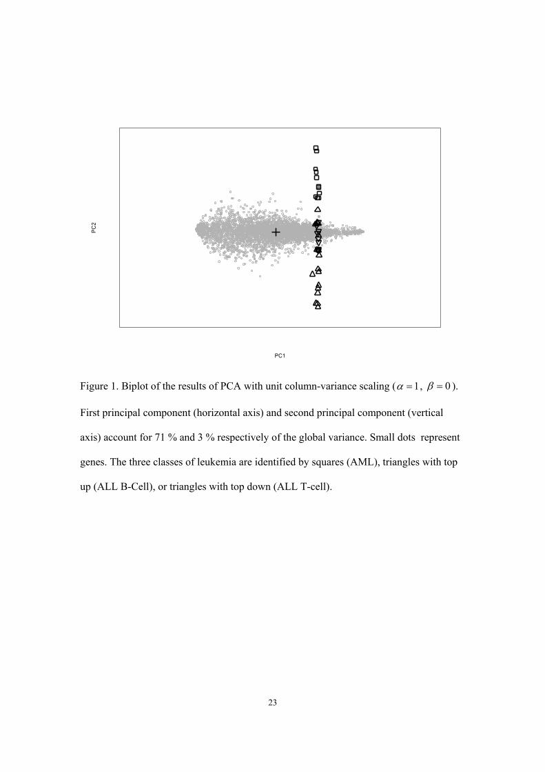
3.1 Principal component analysis
PCA was carried out after logarithmic re-expression of the gene expression profiles in
MIT1. Since gene expression data are positively skewed and can contain large influential
values, we considered a logarithmic re-expression appropriate. For the construction of the
biplot (Figure 1), an asymmetric scaling with unit column-variance ( 1α = , 0β = ) was
used to allow better visual discrimination between the different samples. This special type
of factor scaling was considered optimal for extreme rectangular matrices of microarray
data where variability between the genes (average variance log transformed data = 6.4) is
much higher than between the different samples (average variance = 2). A consequence
of unit column-variance factor scaling is that correlations and distances between samples
are not represented in the biplot. However, in exploring gene expression data only pat-
terns in the distribution of the biological samples are of direct interest. In Figure 1, the
horizontal axis of the biplot, represents the first principal component that accounts for
71% of the total variance in the data. The second principal component is represented by
the vertical axis of the biplot and explains only 3% of the total variance. The remaining
14
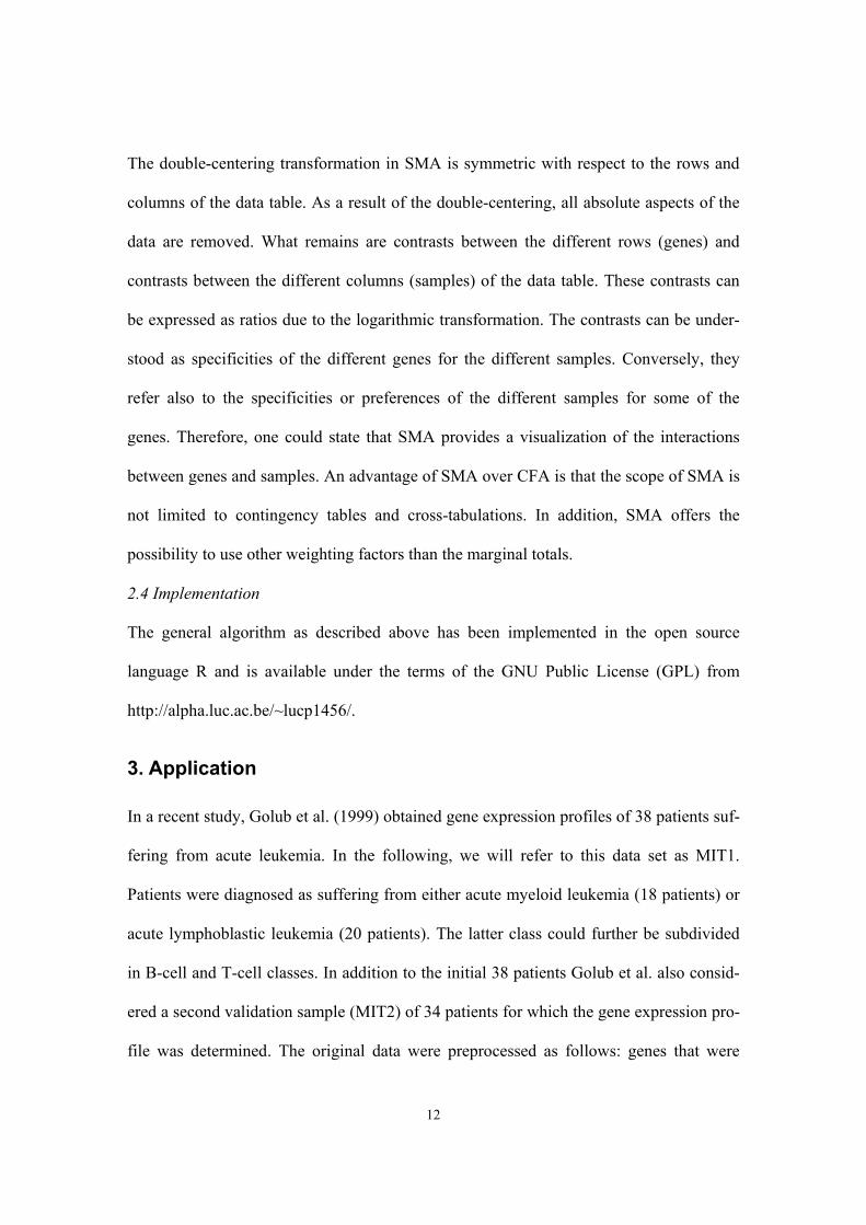
principal components were considered to reflect random disturbances. The horizontal
axis is dominated entirely by a global component related to the size of the measurements
and does not contribute any information about the differential expression of genes in the
samples. Differences between biological samples are found only along the vertical axis.
Only a difference between the ALL and AML groups is eminent, while data from ALL
B-lineage and ALL T-lineage completely overlap one another. Furthermore, it is impos-
sible to use the biplot for selecting genes that discriminate best between the ALL and
AML classes.
=== Figure 1. About here ===
3.2 Correspondence factor analysis
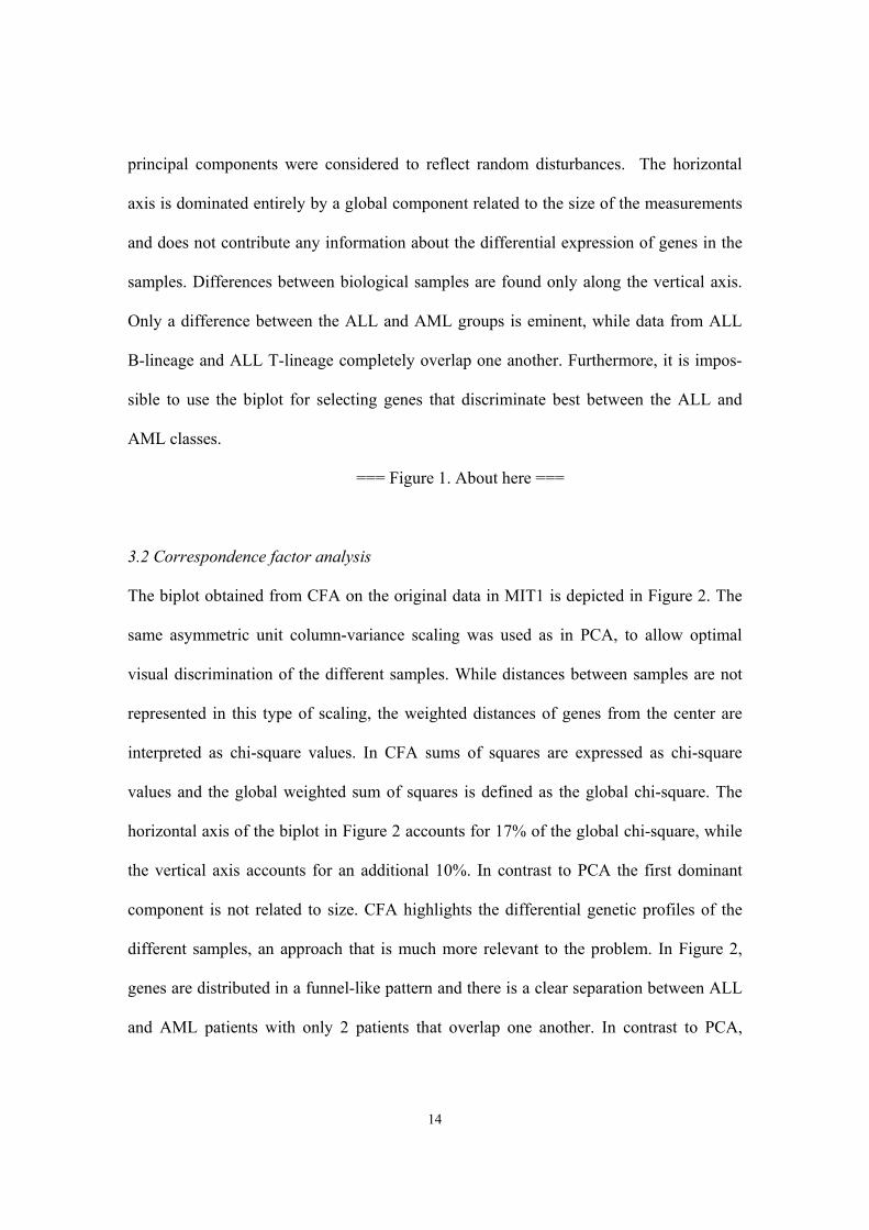
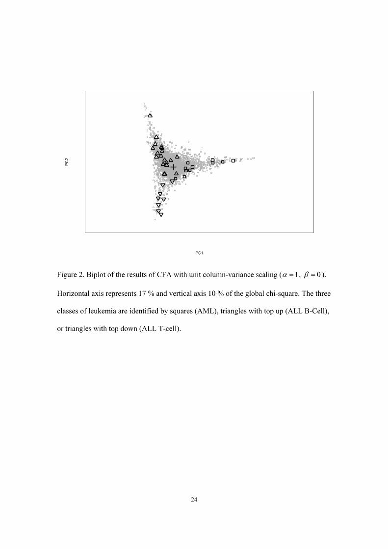
The biplot obtained from CFA on the original data in MIT1 is depicted in Figure 2. The
same asymmetric unit column-variance scaling was used as in PCA, to allow optimal
visual discrimination of the different samples. While distances between samples are not
represented in this type of scaling, the weighted distances of genes from the center are
interpreted as chi-square values. In CFA sums of squares are expressed as chi-square
values and the global weighted sum of squares is defined as the global chi-square. The
horizontal axis of the biplot in Figure 2 accounts for 17% of the global chi-square, while
the vertical axis accounts for an additional 10%. In contrast to PCA the first dominant
component is not related to size. CFA highlights the differential genetic profiles of the
different samples, an approach that is much more relevant to the problem. In Figure 2,
genes are distributed in a funnel-like pattern and there is a clear separation between ALL
and AML patients with only 2 patients that overlap one another. In contrast to PCA,
15
B-lineage and T-lineage classes within the ALL group are also separated from one
another. It is tempting to identify a few genes that could be used in characterizing the
three pathological classes. Gene probes located at the poles of the triangular-like shape
should be characteristic for a given class of leukemia. However, for the two gene probes
identified as the top left and right pole only a few valid measurements were made and the
results depended largely on the expression level obtained in a single patient. This under-
scores the, in this case, less desirable sensitivity of CFA to single large values. There is
also a problem with the interpretation of the numerical value of the distances between
genes. Since in CFA, distances refer to chi-square values that have a meaning only for
contingency tables and not for continuous data as is the case in gene expression experi-
ments, one could seriously question the applicability of CFA in microarray data analysis.
=== Figure 2. About here ===
3.3 Spectral map analysis
In carrying out SMA, we used variable weighting for the genes and samples, with
weights proportional to the mean expression levels of genes and samples respectively.
Asymmetric unit column-variance was used as factor scaling in the construction of the
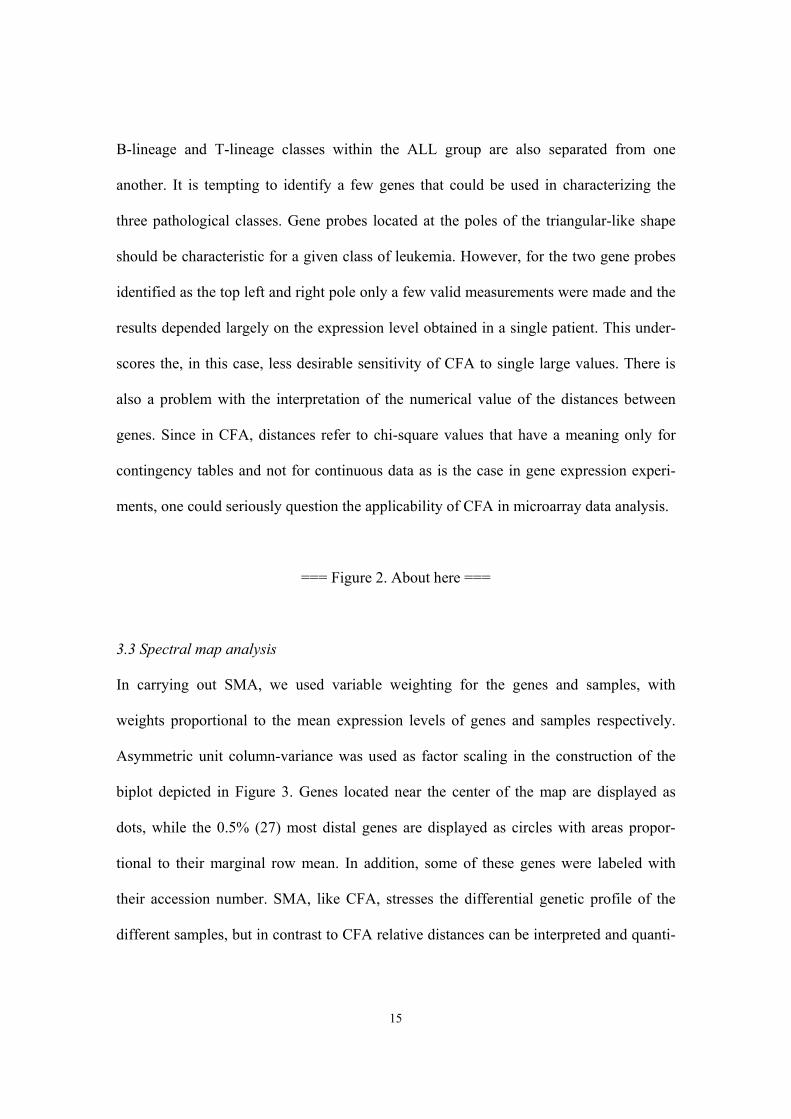
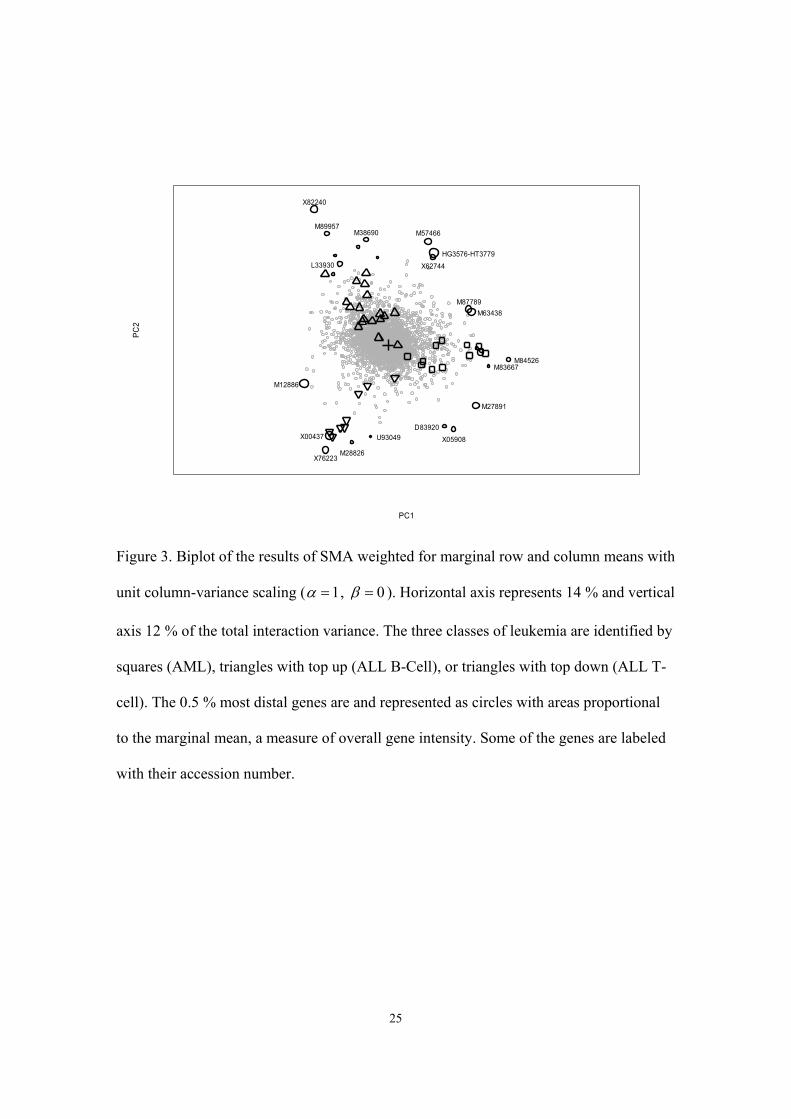
biplot depicted in Figure 3. Genes located near the center of the map are displayed as
dots, while the 0.5% (27) most distal genes are displayed as circles with areas propor-
tional to their marginal row mean. In addition, some of these genes were labeled with
their accession number. SMA, like CFA, stresses the differential genetic profile of the
different samples, but in contrast to CFA relative distances can be interpreted and quanti-

16
fied as ratios. The three classes of leukemia are completely separated from one another
and cluster around the three poles of a triangle. The horizontal axis of the map is domi-
nated by the ratio in gene expression between the AML and ALL class and accounts for
14% of the total interaction variance. The vertical axis is dominated by the contrast
between the ALL T-cell and ALL B-cell group and accounts for an additional 12% of the
interaction. All of the genes that are located distal from the center could have a physio-
logical meaning. It is noteworthy to mention that only 4 of the 27 most distal genes were
among the 50 genes selected by Golub et al. (1999) to discriminate between the different
classes of disease.
=== Figure 3. About here ===
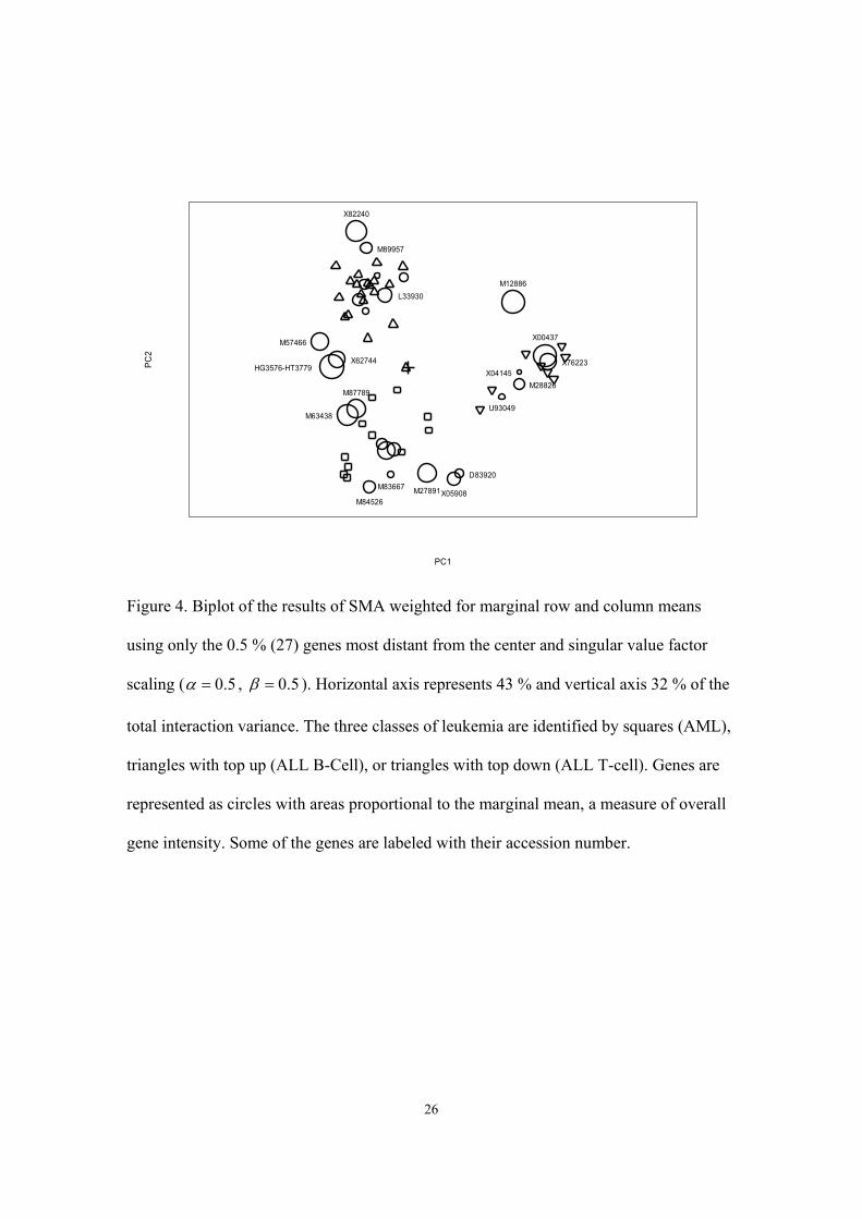
In a subsequent analysis (Fig. 4), we carried out a weighted SMA using the 27 genes
identified in Figure 3. Since row and column variances are now comparable, the biplot
was constructed using singular values ( 0.5α = , 0.5β = ) as the method for factor
scaling. The horizontal and vertical axes explain 43% and 32% of the global interaction
variance. Using only this small subset of 27 genes allows complete separation of the three
pathological classes. To validate this finding, we positioned the samples obtained in the
second data set (MIT2) on the biplot based on MIT1 (results not shown). AML and
ALL-B classes could clearly be distinguished from one another without any overlap.
There was only one possible mismatch, namely the single sample in MIT2 that was
identified as ALL-T.
=== Figure 4. About here ===
17
c. SMA as a tool to quantify differential gene expression
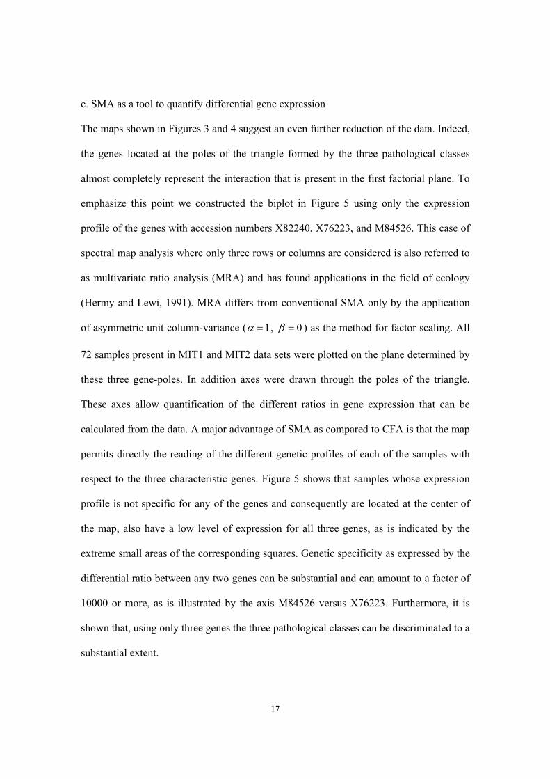
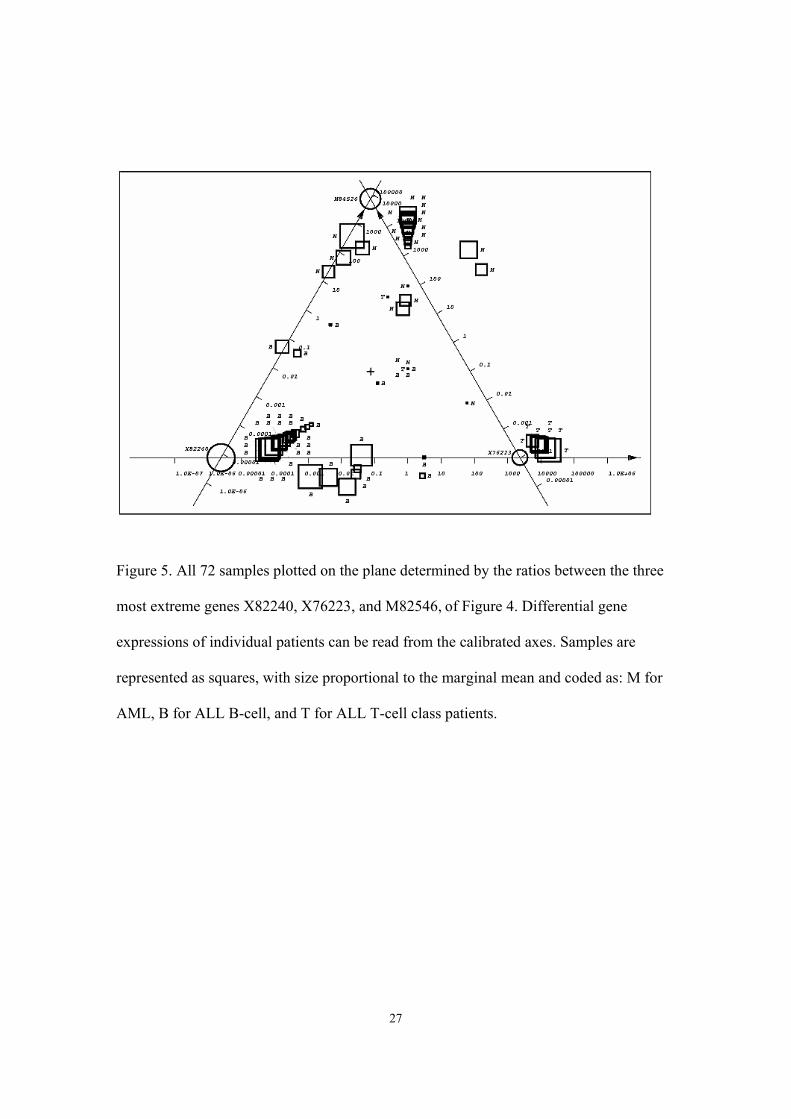
The maps shown in Figures 3 and 4 suggest an even further reduction of the data. Indeed,
the genes located at the poles of the triangle formed by the three pathological classes
almost completely represent the interaction that is present in the first factorial plane. To
emphasize this point we constructed the biplot in Figure 5 using only the expression
profile of the genes with accession numbers X82240, X76223, and M84526. This case of
spectral map analysis where only three rows or columns are considered is also referred to
as multivariate ratio analysis (MRA) and has found applications in the field of ecology
(Hermy and Lewi, 1991). MRA differs from conventional SMA only by the application
of asymmetric unit column-variance ( 1α = , 0β = ) as the method for factor scaling. All
72 samples present in MIT1 and MIT2 data sets were plotted on the plane determined by
these three gene-poles. In addition axes were drawn through the poles of the triangle.
These axes allow quantification of the different ratios in gene expression that can be
calculated from the data. A major advantage of SMA as compared to CFA is that the map
permits directly the reading of the different genetic profiles of each of the samples with
respect to the three characteristic genes. Figure 5 shows that samples whose expression
profile is not specific for any of the genes and consequently are located at the center of
the map, also have a low level of expression for all three genes, as is indicated by the
extreme small areas of the corresponding squares. Genetic specificity as expressed by the
differential ratio between any two genes can be substantial and can amount to a factor of
10000 or more, as is illustrated by the axis M84526 versus X76223. Furthermore, it is
shown that, using only three genes the three pathological classes can be discriminated to a
substantial extent.
18
=== Figure 5. About here ===
4. Discussion
The results obtained in the previous section illustrate the impact of the different building
blocks introduced in Section 2. The characteristic difference between conventional PCA
on the one hand and CFA and SMA on the other hand are the operations of double-
closure and double-centering. The double-closure operation in CFA eliminates the size
factor that is related to the first dominant component in PCA and stresses differences
among the genes and among the samples. The same effect is obtained by double-
centering after logarithmic re-expression in SMA. Although, mathematically, these two
operations are related, the results can differ substantially as is illustrated by the differ-
ences in the biplots obtained from CFA and SMA, respectively. Re-expressing the data to
logarithms downplays very large contrasts that result from extreme outcomes. This is a
desirable property for the analysis of gene expression data that typically suffer from the
presence of severely outlying measurements. A drawback of the logarithmic re-
expression is that contrasts at a less reliable level of gene expression are considered of
equal importance as are contrasts at a more reliable level. This phenomenon can be
counteracted by incorporating weights proportional to the marginal totals in the centering,
normalization, and factorization building blocks leading to weighted SMA.
Our results indicate that weighted SMA is a valuable tool for the analysis of gene expres-
sion microarray data. Weighted SMA and CFA outperform conventional PCA in visual-
izing the data, determining clusters of samples and genes, correlating samples with gene
19
expression profiles, and reducing the data. An advantage of SMA over CFA is the possi-
bility of interpreting distances as ratios, while CFA does not allow such an intuitive
approach. A limitation with regard to interpretation of the spectral map would be the
abundance of groupings in the different samples as is the case in some data mining appli-
cations. However, for such applications one could consider exploring subsets of the data
instead of entire data sets.
Apart from the data analytic aspects of this report, it is noteworthy to mention that the
three genes selected in the construction of Figure 5, could be related to leukemia. Only
“Adipsin” (M84526) was also present in the set of 50 genes used by Golub et al. (1999)
for class determination. This gene was also identified by an alternative analysis of the
same data set reported by Chow, Moler, and Mian (2001). The second gene “T-cell
leukemia/lymphoma 1A” (X82240) is reported to be involved in T-cell malignancies
(Virgilio et al., 1994). The last gene probe (X76223) measures the presence of exon 4 of
the gene “MAL”, which encodes a human T-cell specific proteolipid protein (Rancano et
al., 1994).
Acknowledgements
We gratefully acknowledge support from the Belgian IUAP/PAI network “Statistical
Techniques and Modeling for Complex Substantive Questions with Complex Data”. The
authors are also thankful to the anonymous reviewer and the associate editor for their
help in improving the manuscript.
20
References
Andries, K., Dewindt, B., Snoeks, J., Wouters, L., Moereels, H., Lewi, P.J., Janssen,
P.A.J. (1990). Two groups of rhinoviruses revealed by a panel of antiviral compounds
present sequence divergence and differential pathogenicity. Journal of Virology 64,
1117-1123.
Benzécri, J.P. (1973). L’analyse des données. Vol II. L’Analyse des Correspondences.
Gounod, Paris.
Chapman, S., Schenk, P., Kazan, K., Manners, J. (2001). Using biplots to interpret gene
expression patterns in plants. Bioinformatics 18, 202-204.
Chow, M.L., Moler, E.J., Mian, I.S. (2001). Identifying marker genes in transcription
profiling data using a mixture of feature relevance experts. Physiological Genomics 5,
99-11.
Eisen, M.B., Spellman, P.T., Brown, P.O., Botstein, D. (1998). Cluster analysis and
display of genome-wide expression patterns. Proceedings of the National Academy of
Sciences USA 95, 14863-14868.
Faes, W., Lewi, P.J. (1987). Spectramap: the story behind your numbers. The
International Management Development Review 3, 183-187.
Fellenberg, K., Hauser, N., Brors, B., Neutzner, A., Hoheisel, J., Vingron, M. (2001).
Correspondence analysis applied to microarray data. Proceedings of the National
Academy of Sciences USA 98, 10781-10786.
Gabriel, K.R. (1971). The biplot graphical display of matrices with applications to
principal component analysis. Biometrika 58, 453-467.

21
Golub, T.R., Slonim, D.K., Tamayo, P., Huard, C., Gaasenbeek, M., Mesirov, J.P.,
Coller, H., Loh, M.L., Downing, J.R., Calgiuri, M.A., Bloomfield, C.D., Lander, E.S.
(1999). Molecular classification of cancer: Class discovery and class prediction by
gene expression monitoring. Science 286, 531–537.
Greenacre, M.J. (1984). Theory and Applications of Correspondence Analysis. Academic
Press, London.
Hermy, M., Lewi, P.J. (1991). Multivariate ratio analysis, a graphic method for
ecological ordination. Ecology 72, 735-738.
Hilsenbeck S.G., Friedrichs, W.E., Schiff, R., O'Connell, P., Hansen, R.K.,
Osborne,C.K., Fuqua, S.A. (1999). Statistical analysis of array expression data as
applied to the problem of tamoxifen resistance. Journal of the National Cancer
Institute 91, 453-459.
Hotelling, H. (1933). Analysis of a complex of statistical variables into principal
components. Journal of Educational Psychology 24, 417-441.
Landgrebe, J., Welzl, G., Metz, T., van Gaalen, M.M., Ropers, H., Wurst, W., Holsboer,
F. (2002). Molecular characterisation of antidepressant effects in the mouse brain
using gen expression profiling. Journal of Psychiatric Research 36, 119-129.
Lefkovits, I., Kuhn, L., Valiron, O., Merle, A., Kettman,J. (1988). Toward an objective
classification of cells in the immune system Proceedings of the National Academy of
Sciences USA 85, 3565–3569.
Lewi, P.J. (1976). Spectral mapping, a technique for classifying biological activity
profiles of chemical compounds. Arzneimittel Forschung (Drug Research) 26, 1295-
1300.

22
Lewi, P.J., Moereels, R. (1994). Receptor mapping and phylogenetic clustering. In:
Advanced Computer-assisted Techniques of Drug Discovery. H. van de Waterbeemd
(Ed.), VCH, Weinheim, Germany, pp. 131-162.
Pearson, K. (1901). On lines and planes of closest fit to points in space. Philosophical
Magazine 2, 559-572.
Rancano, C., Rubio, T., Correas, I., Alonso, M.A. (1994). Genomic structure and
subcellular localization of MAL, a human T-cell-specific proteolipid protein. Journal
of Biological Chemistry 269, 8159-8164.
Tavazoie, S., Hughes, J.D., Campbell, M.J., Cho, R.J.,Church , G.M. (1999). Systematic
determination of genetic network architecture. Nature Genetics 22, 281-285.
Thielemans,A., Lewi,P.J., Massart, D.L. (1988). Similarities and differences among
multivariate display techniques illustrated by Belgian cancer mortality distribution
data. Chemometrics and Intelligent Laboratory Systems 3, 277-300.
Törönen, P., Kolehmainen, M., Wong, G., Castrén, E. (1999). Analysis of gene
expression data using self-organizing maps. FEBS Letters 451, 142-146.
Virgilio, L., Narducci, M.G., Isobe, M., Billips, L.G., Cooper, M.D., Croce, C.M., Russo,
G. (1994). Identification of the TCL1 gene involved in T-cell malignancies.
Proceedings of the National Academy of Sciences USA 91, 12530-12534.
23
PC1
PC2
Figure 1. Biplot of the results of PCA with unit column-variance scaling ( 1α = , 0β = ).
First principal component (horizontal axis) and second principal component (vertical
axis) account for 71 % and 3 % respectively of the global variance. Small dots represent
genes. The three classes of leukemia are identified by squares (AML), triangles with top
up (ALL B-Cell), or triangles with top down (ALL T-cell).
24
PC1
PC2
Figure 2. Biplot of the results of CFA with unit column-variance scaling ( 1α = , 0β = ).
Horizontal axis represents 17 % and vertical axis 10 % of the global chi-square. The three
classes of leukemia are identified by squares (AML), triangles with top up (ALL B-Cell),
or triangles with top down (ALL T-cell).
25
PC1
PC2
D83920
HG3576-HT3779L33930
M12886
M27891
M28826
M38690 M57466
M63438
M83667M84526
M87789
M89957
X00437 X05908
X62744
X76223
X82240
U93049
Figure 3. Biplot of the results of SMA weighted for marginal row and column means with
unit column-variance scaling ( 1α = , 0β = ). Horizontal axis represents 14 % and vertical
axis 12 % of the total interaction variance. The three classes of leukemia are identified by
squares (AML), triangles with top up (ALL B-Cell), or triangles with top down (ALL T-
cell). The 0.5 % most distal genes are and represented as circles with areas proportional
to the marginal mean, a measure of overall gene intensity. Some of the genes are labeled
with their accession number.
26
PC1
PC2
D83920
HG3576-HT3779
L33930M12886
M27891
M28826
M57466
M63438
M83667
M84526
M87789
M89957
U93049
X00437
X04145
X05908
X62744 X76223
X82240
Figure 4. Biplot of the results of SMA weighted for marginal row and column means
using only the 0.5 % (27) genes most distant from the center and singular value factor
scaling ( 0.5α = , 0.5β = ). Horizontal axis represents 43 % and vertical axis 32 % of the
total interaction variance. The three classes of leukemia are identified by squares (AML),
triangles with top up (ALL B-Cell), or triangles with top down (ALL T-cell). Genes are
represented as circles with areas proportional to the marginal mean, a measure of overall
gene intensity. Some of the genes are labeled with their accession number.
27
Figure 5. All 72 samples plotted on the plane determined by the ratios between the three
most extreme genes X82240, X76223, and M82546, of Figure 4. Differential gene
expressions of individual patients can be read from the calibrated axes. Samples are
represented as squares, with size proportional to the marginal mean and coded as: M for
AML, B for ALL B-cell, and T for ALL T-cell class patients.
Copyright © 2022 FDOKUMEN