A comparative study of accuracy of shock capturing schemes for simulation of shock/acoustic wave...

aeroacousticsvolume 13 · number 3 & 4 · 2014

A comparative study of accuracy of shockcapturing schemes for simulation of

shock/acoustic wave interactions

by

Dmitry V. Khotyanovsky, Alexey N. Kudryavtsev and Andrey Yu. Ovsyannikov

reprinted from

published by MULTI-SCIENCE PUBLISHING CO. LTD.,

5 Wates Way, Brentwood, Essex, CM15 9TB UK

E-MAIL: [email protected]

WEBSITE: www.multi-science.co.uk

aeroacoustics volume 13 · number 3 & 4 · 2014 – pages 261 – 274 261

A comparative study of accuracy of shockcapturing schemes for simulation of

shock/acoustic wave interactions

Dmitry V. Khotyanovsky1,2, Alexey N. Kudryavtsev1,2 and AndreyYu. Ovsyannikov3

1Khristianovich Institute of Theoretical and Applied Mechanics, Siberian Branch of the Russian

Academy of Sciences, 4/1, Institutskaya st., Novosibirsk, 630090, Russia

[email protected], [email protected] State University, 2, Pirogova st., Novosibirsk, 630090, Russia

3Center for Turbulence Research, 488 Escondido Mall Building 500, Stanford University, Stanford,

CA 94305-3024, USA

[email protected]

Received May 1, 2013; Revised April 21, 2014; Accepted May 1, 2014

ABSTRACTWe simulate transmission of a small-amplitude disturbance wave through a shock wave. Results ofour numerical experiments performed with different high-order shock-capturing schemes show thatthe capability of a scheme to correctly predict the amplification of the disturbances crucially dependson the Riemann solver used in evaluation of numerical fluxes. Incorrectly high amplification rates areproduced by the solvers resolving shock waves sharply, with no interior points in numerical profilesof steady shock waves. In particular, both the exact Riemann solver and the popular Roe fluxdifference splitting demonstrate such unphysical behavior. A possible explanation of such behavior isproposed. More dissipative solvers, such as the global Lax–Friedrichs splitting, produce transmissioncoefficients close to the predictions of linear theory.

1. INTRODUCTIONInteraction of small disturbances, such as acoustic waves, with a shock wave is relevantto many fundamental problems and applications of aeroacoustics in supersonic flows.For example, shock wave interactions with near-wall boundary layers and free shearflows result in a significant increase in intensity of turbulent fluctuations1,2.

When the flow disturbance amplitude is small, linear interaction analysis (LIA) canbe used to predict the amplification rate. In the elementary case of normal incidence ofsound on the shock wave, this was done independently by Blokhintsev3 and Burgers4

for the problem of a sound receiver in a supersonic flow. The general case of theinclined incidence of an acoustic wave on a shock wave was considered later in a seriesof papers. The complete solution of the problem was obtained by Dyakov5,6, who

considered stationary disturbances, and by Kontorovitch7 for disturbances in the formof a propagating wave. The most complete linear theory is presented in Ref. 8, wherethe solution for a fluid with an arbitrary equation of state was obtained, and is alsodiscussed in Ref. 9.

For disturbances of large amplitudes the linear theory is no longer valid, and theonly possible tool of prediction is the direct numerical simulation. Numericalsolvers used for this purpose are required to be highly accurate and capture flowdiscontinuities robustly. Modern shock capturing schemes are the powerful tool fornumerical simulation of the flows containing gas dynamic discontinuities. Theseschemes typically use high-order TVD (total variation diminishing) or ENO(essentially non-oscillatory) reconstruction of the flow variables, and solve theRiemann problem between two states to obtain the numerical flux on the cellinterface. However, despite the multitude of impressing results obtained with theiruse, exact mathematical theory of such schemes is still missing. It is well knownthat in some cases they demonstrate pathological behavior (e.g., carbunclephenomenon), and their order of convergence in simulation of flows withdiscontinuities does not generally correspond to the theoretical order obtained inassumption of a smooth solution.

The purpose of the present study is to investigate capabilities of the differentnumerical schemes to correctly predict the properties of the disturbance wavetransmitted through the shock wave in a few simple model configurations, where theLIA can be applied.

2. NUMERICAL METHODSIn this study we solve numerically 1D and 2D Euler and Navier–Stokes equations withseveral different numerical methods.

The first method is a MUSCL TVD algorithm which utilizes either the 2nd orderpurely upwind or 4th order (Yamamoto & Daiguji10) reconstruction of primitivevariables (density, velocity and pressure) on cell faces from their values in cellcenters. The reconstructed variables are limited using the “minmod” slope limiterto avoid numerical oscillations near flow discontinues. For the 4th order scheme thelimiting procedure is invoked twice as described in Ref. 10. The numerical fluxeson cell interface are then evaluated from the “left” and “right” reconstructed flowvariables solving the Riemann problem between left and right state. The Riemannsolvers used in our numerical experiments are the exact iterative Riemann solver ofGodunov11, Roe flux difference splitting12 with entropy fix13, and van Leer fluxvector splitting14.

Another class of upwind schemes, which is more attractive to simulate transitionand turbulence in high-speed flows, is the ENO (essentially non-oscillatory) andWENO (weighted ENO) schemes. The ENO schemes use an adaptive “smoothest”sub-stencil chosen within a larger, fixed stencil to construct high-orderapproximation of the solution avoiding the interpolation across discontinuities andpreserving uniformly high-order accuracy everywhere where the solution is

262 A comparative study of accuracy of shock capturing schemes for

simulation of shock/acoustic wave interactions

smooth. The main idea of the WENO schemes is to use a superposition of severalsub-stencils with adaptive coefficients to increase the order of approximation evenmore. In this paper we employ the finite-difference, flux-based, 5th order WENOscheme of Jiang & Shu15. The Riemann solvers tested with this numerical algorithmare the Roe flux difference splitting, and more dissipative Lax–Friedrichs fluxsplitting15. In this study we use two different formulations of the Lax–Friedrichsflux splitting: local Lax–Friedrichs (LLF) and global Lax–Friedrichs (GLF). Thedifference between the two is that the former use local maxima of the eigenvaluesof the Lax–Friedrics coefficients, whereas the latter searches for maxima over theentire range of eigenvalues in the computational domain. The GLF is moredissipative and robust at strong shocks.

In order to eliminate the effects of the shock-capturing schemes on transmission ofthe acoustic waves through the gas dynamic discontinuity we solve a reference casewith the Navier–Stokes equations resolving the internal structure of the smooth viscousshock wave transition. In this case the scale parameter is the ratio of the disturbancewavelength l to the width of the viscous shock transition d: as l/d tends to infinity, theviscous Navier–Stokes solution should converge to the solution of an inviscid problem.Since there are no discontinuities in this viscous problem, any high-order low-dissipative method can be used. We choose upwind-biased compact differences16 of the5th order for discretization of convective terms of the Navier–Stokes equations andcentral, 6th order compact differences17 for diffusive terms.

Time integration is performed with the 4th order explicit low-storageRunge–Kutta–Gill algorithm18. Time step is automatically adjusted to satisfy the globalCFL condition with the maximum Courant number 0.7.

3. RESULTS AND DISCUSSION3.1. Acoustic wave propagation in a uniform supersonic flowTo investigate basic properties of the shock-capturing schemes used herein, we firstconsider their capabilities at a problem without shocks. For this purpose, weperformed 1D Euler simulations of propagation of a plane monochromatic soundwave in a uniform supersonic flow. Linear analytical solution of this problem can befound in textbooks (e.g., Ref. 19). We consider a fast acoustic wave travelling at thespeed u+c, where u is the flow velocity and c is the speed of sound. At inflow, atime-periodic acoustic disturbance with pressure amplitude dp = 1·10-4 was imposedon the uniform flow with the Mach number M = 8. Size of the computational domainwas 5 wavelenghts l of the disturbance wave. Uniform grids with 200 cells per lwere used.

Results of these computations are presented in Fig. 1. As seen in Fig. 1a, thecomputations with the 5th order WENO scheme perfectly reproduce the sine waveof the propagating acoustic disturbance. Since the solution is smooth, the WENO-5 uses the entire stencil and should actually have the 5th order of approximation inthe entire domain. Though the number of grid cells per l is relatively moderate, thesymbols representing the numerical solution are visually indistinguishable from the

aeroacoustics volume 13 · number 3 & 4 · 2014 263



Figure 1: Pressure fluctuations for the propagation of a sound wave in auniform M = 8 flow: WENO-5 solution in the entire domain (a);close-up of a local maximum computed with WENO-5 (b), 4th orderMUSCL TVD (c), and 2nd order MUSCL TVD (d). Solid sine curvecorresponds to the analytical solution.

x/λ

(p-p

∞)/

p ∞

0 1 2 3 4 5−1E-04

−5E-05

0

5E-05

0.0001(a)

(p-p

∞)/

p ∞

2.1 2.2 2.3 2.4x/λ

8.5E-05

9E-05

9.5E-05

0.0001(p

-p∞)/

p ∞

8.5E-05

9E-05

9.5E-05

0.0001

2.1 2.2 2.3 2.4x/λ

(b) (c)

(p-p

∞)/

p ∞

8.5E-05

9E-05

9.5E-05

0.0001

2.1 2.2 2.3 2.4x/λ

(d)

solid curve corresponding to the analytical solution, which is especially evident inthe enlarged region of the wave crest shown in Fig. 1b.

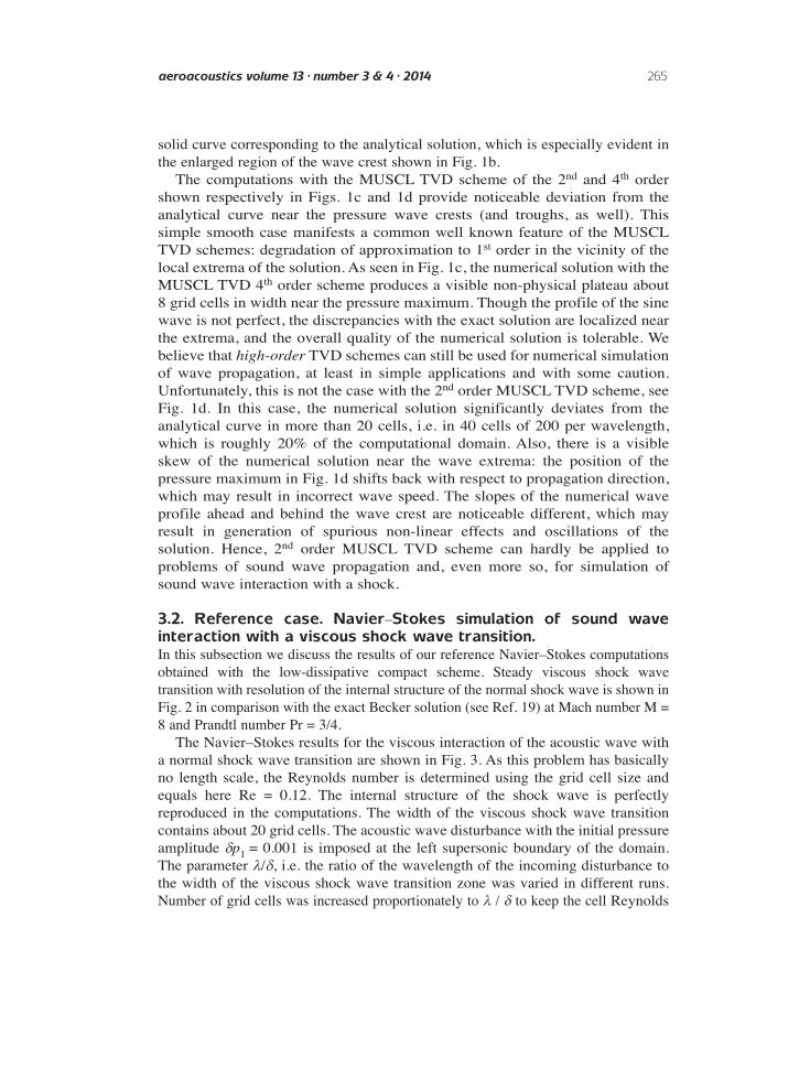
The computations with the MUSCL TVD scheme of the 2nd and 4th ordershown respectively in Figs. 1c and 1d provide noticeable deviation from theanalytical curve near the pressure wave crests (and troughs, as well). Thissimple smooth case manifests a common well known feature of the MUSCLTVD schemes: degradation of approximation to 1st order in the vicinity of thelocal extrema of the solution. As seen in Fig. 1c, the numerical solution with theMUSCL TVD 4th order scheme produces a visible non-physical plateau about8 grid cells in width near the pressure maximum. Though the profile of the sinewave is not perfect, the discrepancies with the exact solution are localized nearthe extrema, and the overall quality of the numerical solution is tolerable. Webelieve that high-order TVD schemes can still be used for numerical simulationof wave propagation, at least in simple applications and with some caution.Unfortunately, this is not the case with the 2nd order MUSCL TVD scheme, seeFig. 1d. In this case, the numerical solution significantly deviates from theanalytical curve in more than 20 cells, i.e. in 40 cells of 200 per wavelength,which is roughly 20% of the computational domain. Also, there is a visibleskew of the numerical solution near the wave extrema: the position of thepressure maximum in Fig. 1d shifts back with respect to propagation direction,which may result in incorrect wave speed. The slopes of the numerical waveprofile ahead and behind the wave crest are noticeable different, which mayresult in generation of spurious non-linear effects and oscillations of thesolution. Hence, 2nd order MUSCL TVD scheme can hardly be applied toproblems of sound wave propagation and, even more so, for simulation ofsound wave interaction with a shock.

3.2. Reference case. Navier–Stokes simulation of sound waveinteraction with a viscous shock wave transition.In this subsection we discuss the results of our reference Navier–Stokes computationsobtained with the low-dissipative compact scheme. Steady viscous shock wavetransition with resolution of the internal structure of the normal shock wave is shown inFig. 2 in comparison with the exact Becker solution (see Ref. 19) at Mach number M =8 and Prandtl number Pr = 3/4.

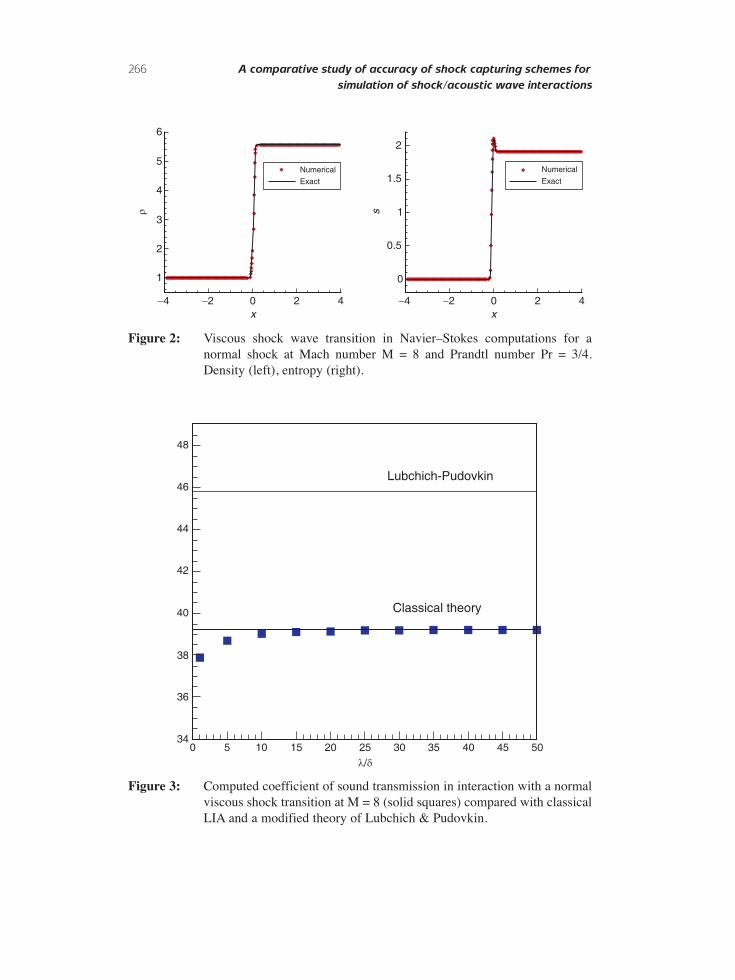
The Navier–Stokes results for the viscous interaction of the acoustic wave witha normal shock wave transition are shown in Fig. 3. As this problem has basicallyno length scale, the Reynolds number is determined using the grid cell size andequals here Re = 0.12. The internal structure of the shock wave is perfectlyreproduced in the computations. The width of the viscous shock wave transitioncontains about 20 grid cells. The acoustic wave disturbance with the initial pressureamplitude dp1 = 0.001 is imposed at the left supersonic boundary of the domain.The parameter l/d, i.e. the ratio of the wavelength of the incoming disturbance tothe width of the viscous shock wave transition zone was varied in different runs.Number of grid cells was increased proportionately to l / d to keep the cell Reynolds




Figure 3: Computed coefficient of sound transmission in interaction with a normalviscous shock transition at M = 8 (solid squares) compared with classicalLIA and a modified theory of Lubchich & Pudovkin.

Figure 2: Viscous shock wave transition in Navier–Stokes computations for anormal shock at Mach number M = 8 and Prandtl number Pr = 3/4.Density (left), entropy (right).

ρ

x

6

5

Exact

Numerical

420−2

4

3

2

1

−4

s

x

Exact

Numerical

420−2−4

2

1.5

0.5

1

0

Lubchich-Pudovkin

Classical theory

λ/δ0 5 10 15 20 25 30 35 40 45 50

34

36

38

40

42

44

46

48

number constant and maintain proper resolution of the shock wave structure. Theresults of the Navier–Stokes simulation of the sound wave transmission throughthe viscous shock transition zone presented in Fig. 3 demonstrate clear trend of thecomputed transmission coefficient dp2/dp1towards the value 39.2272 predicted bythe classical linear interaction analysis7,8 as the parameter l/d increases. Forcomparison, the prediction of a recently proposed alternative theory20 shown in Fig.3 greatly disagrees with the results of the computations and predictions of theclassical LIA. More quantitatively, the results of the convergence of theNavier–Stokes data to linear theory predictions are given in Table 1, where welisted the computed values of dp2/dp1 and the relative error of the numericalcomputations in a broad range of l/d. Table 1 clearly shows that, as l/d increases,the results of viscous computations tend to the inviscid limit with the accuracy of0.0002 %.

3.3. Acoustic wave interaction with a steady normal shock. Inviscidsimulations with several shock capturing schemesTo investigate capabilities of different shock-capturing schemes to predict amplificationof the disturbance wave passing through a shock wave we performed numericalsimulations for the one-dimensional problem. We consider the interaction of a fastacoustic wave with an amplitude dp1 = 1·10–4 impinging on a steady normal shock.Linear solution for this problem was obtained by Blokhintsev3 and Burgers4, and isdiscussed in Ref. 21.

The flow Mach number is varied between M = 2 and M = 8. The perfect gas with thespecific heat ratio g = 1.4 is considered. The length of the computational domain was 5wavelengths l of the oncoming disturbance. The normal shock was located at x/l =1.The grid was uniform with 200 cells per l.

Figure 4 presents steady pressure profiles across the shock obtained with differentsolvers at M = 8. The exact Godunov and Roe solvers yield a pressure jump with nointerior points, whereas more diffusive van Leer and global Lax–Friedrichs splittingsproduce a smeared shock wave with two and four interior points, respectively.


Table 1: Convergence of the numerically predicted transmission coefficientdp2/dp1 to its theoretical value of 39.2272 with increase of the parameter l/d

l/d dp2/dp1 Relative error, %

1 37.90 3.385 38.69 1.3610 39.01 0.5520 39.145 0.2030 39.190 0.09450 39.212 0.038100 39.2235 0.009500 39.2271 0.0002

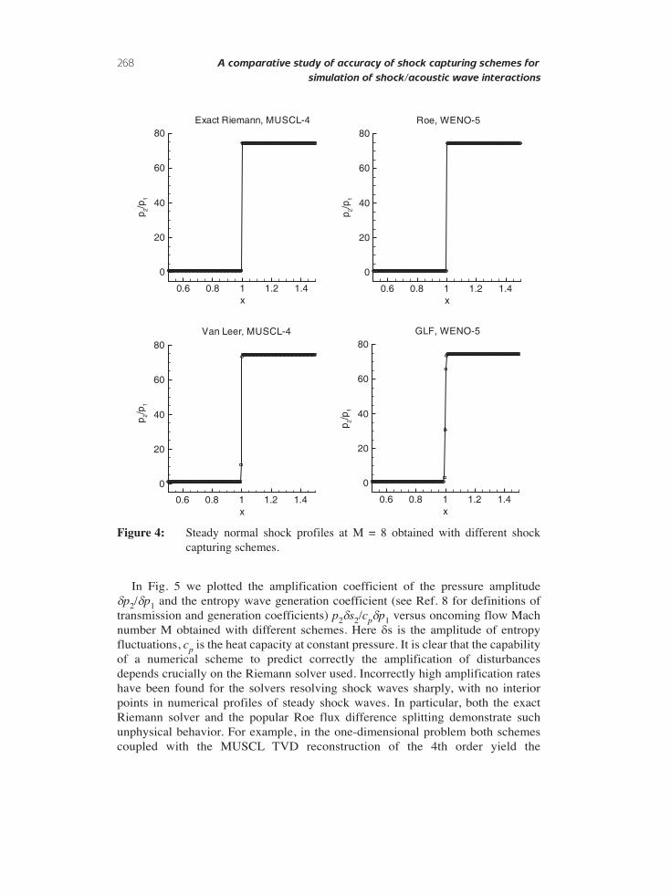
In Fig. 5 we plotted the amplification coefficient of the pressure amplitudedp2/dp1 and the entropy wave generation coefficient (see Ref. 8 for definitions oftransmission and generation coefficients) p2ds2/cpdp1 versus oncoming flow Machnumber M obtained with different schemes. Here ds is the amplitude of entropyfluctuations, cp is the heat capacity at constant pressure. It is clear that the capabilityof a numerical scheme to predict correctly the amplification of disturbancesdepends crucially on the Riemann solver used. Incorrectly high amplification rateshave been found for the solvers resolving shock waves sharply, with no interiorpoints in numerical profiles of steady shock waves. In particular, both the exactRiemann solver and the popular Roe flux difference splitting demonstrate suchunphysical behavior. For example, in the one-dimensional problem both schemescoupled with the MUSCL TVD reconstruction of the 4th order yield the



x

p 2/p 1

0

20

40

60

80Exact Riemann, MUSCL-4

0.6 0.8 1 1.2 1.4

Van Leer, MUSCL-4

0

20

40

60

80

0.6 0.8 1 1.2 1.4x

Roe, WENO-5

0

20

40

60

80

0.6 0.8 1 1.2 1.4x

p 2/p 1

x

GLF, WENO-5

0

20

40

60

80

0.6 0.8 1 1.2 1.4

p 2/p 1

p 2/p 1

Figure 4: Steady normal shock profiles at M = 8 obtained with different shockcapturing schemes.

amplification rates of acoustic disturbances close to 300 instead of the theoreticalvalue of 39.2 for a Mach 8 shock wave.

It is a surprising result since the less dissipative approximate Riemann solver ofRoe is widely accepted as the most appropriate for simulation of wave-dominatedflows encountered in aeroacoustics, boundary layer transition, etc. Such unphysicalamplification rates may be connected to the numerical generation of longwavelength noise downstream of a slowly moving shock wave, which was


Mach number

Pre

ssur

e w

ave

ampl

ifica

tion

1 2 3 4 5 6 7 80

10

20

30

40

50

60

70

80

90

100

Mach number

Ent

ropy

wav

e ge

nera

tion

0

10

20

30

40

50

60

70

80

90

100

LLF, WENO-5Roe, WENO-5

AnalyticalGodunov, MUSCL-4Roe, MUSCL-4Van Leer, MUSCL-4GLF, WENO-5

1 2 3 4 5 6 7 8

LLF, WENO-5Roe, WENO-5

AnalyticalGodunov, MUSCL-4Roe, MUSCL-4Van Leer, MUSCL-4GLF, WENO-5

Figure 5: Pressure amplification and entropy wave generation coefficients obtainedwith several different shock capturing schemes compared to theanalytical solution.

observed in some numerical works (see, e.g. Ref. 22). This phenomenon is causedby periodic variations of the numerical (smeared) shock wave profile, in particular,by increase and decrease in its thickness while the shock wave moves with respectto grid nodes. The dominating frequency of generated perturbations is D/Dx, whereD is the shock wave velocity and Dx is the grid cell size. A rapidly moving shockwave generates high-frequency oscillations which are effectively suppressed by thenumerical viscosity inherent in shock capturing methods. However, the numericalviscosity hardly affects low-frequency, long-wavelength perturbations emanatedfrom a slowly moving shock waves and they are distinctively visible behind it.

In our simulations the shock wave oscillates around the stationary position changingits location with respect to the grid under action of the incident acoustic wave. Thevelocity of this forth-and-back movement is D = 4 dA/T where dA is the maximumdisplacement of shock wave from its stationary position and T is the period of theincident acoustic wave. If the amplitude of the acoustic wave is small then dA is smalltoo and the shock wave moves slowly. As a result, it generates unphysical long-wavelength disturbances which are added to physical transmitted waves.

On the other side, more diffusive Riemann solvers, which produce shock waveprofiles smeared over 3–4 grid cells, predict the amplification rate of small disturbancesmuch better. The van Leer flux vector splitting amplification rates are close to thetheoretical curves at low Mach numbers, but tend to deviate as the Mach number grows.The LLF solver produces almost perfect pressure wave amplification, but its entropygeneration is unfortunately much higher than the theoretical curve. We found that closeagreement with LIA predictions has been obtained using the 5th order WENO schemewith the global Lax–Friedrichs splitting. The results of these computations arepresented in Fig. 6, where the pressure amplitude of the acoustic disturbance interactingwith the Mach 8 shock is plotted. It is clear that the transmitted wave amplitude is close



x/λ

−1.0E-04

−5.0E-05

0.0E+00

5.0E-05

1.0E-04

0 0.2 0.4 0.6 0.8 1−4.0E-03

−2.0E-03

0.0E+00

2.0E-03

4.0E-03

2 3 4 5x/λ

Figure 6: Pressure amplitude of an acoustic wave interacting with a Mach 8shock wave obtained with WENO-5 GLF scheme. Shock waveposition is x/l = 1. Dashed lines correspond to the amplification rate39.2 predicted by the LIA.

to the LIA prediction of 39.2 for the pressure wave amplification. Some high-frequencyoscillations are visible in the right plot of Fig. 6 just behind the shock wave located atx/l = 1. Although these oscillations are apparently confined within a half-wavelengthof the transmitted wave downstream of the shock wave, they may be the reason ofslightly lower amplitude of the transmitted pressure wave.

It can be assumed that the better accuracy of the more diffusive solvers is explainedby the fact that the smeared shock wave profile produced by them changes only slightlywhen the shock wave moves with respect to the grid so that the amplitude of generatedunphysical perturbation is quite small.

3.3. Acoustic wave interaction with a steady oblique shock in asupersonic flowTwo-dimensional computations were performed with an acoustic wave interacting withan oblique shock wave. A comparison of theoretical amplification rates with thoseobtained using WENO-5 GLF is given in Fig. 7, where the ratio of the pressuredisturbance amplitudes behind and ahead of an oblique shock wave is shown as afunction of the disturbance incidence angle. The computations are performed for theacoustic waves of amplitude dp1 = 1·10-4 propagating in a supersonic Mach 8 flow andinteracting with a shock inclined at the angle a = 35° to the oncoming flow.


Angle of incidence

δp2/δp

1

0 20 40 60 800

5

10

15

20

Figure 7: Pressure amplification rates of an acoustic wave interacting with an obliqueshock wave with angle 35° in Mach 8 flow for different angles of incidenceof the disturbance wave. Solid line corresponds to the LIA prediction.

LIA transmission coefficients corresponding to this case were obtained using theanalytical formulation given in Ref.6. The angle of the propagation of the acoustic wavewas varied in the different computations. It is clear that the amplification rate is closeto the linear theory prediction though deviation of the numerically computedamplifications is observed at some angles of incidence.

4. CONCLUSIONOur numerical experiments performed with different high-order shock-capturingflow solvers suggest that the choice of a Riemann solver used in evaluatingnumerical fluxes is extremely important for correct simulation of the transmissionof the small-amplitude acoustic disturbance wave through a shock. Both the exactRiemann solver and the Roe flux splitting produce amplification rates that are muchhigher than those predicted by the linear interaction analysis. This discrepancytends to grow with increasing the Mach number. More diffusive Riemann solversgive amplification rates in much closer agreement with the theory. We found thatthe global Lax–Friedrichs flux splitting is especially reliable in solving suchproblems, which was also confirmed in our two-dimensional simulations. Adrawback of the global Lax–Friedrichs solver is that its amplification rates areslightly lower than theoretical.

The observed deficiency of the less dissipative Riemann solvers requires thoroughinvestigation. A possible reason for the non-physical amplification of the disturbancewave may be the noise generation mechanism in slowly moving shocks reported inprevious studies22.

ACKNOWLEDGMENT. Two first authors (D.K and A.K) would like to acknowledge the support from theRussian Government via Grant 14.Z50.31.0019 for conducting research undersupervision of leading scientists. The work was also partially supported by theRussian Foundation for Basic Research (Project No. 12-01-00840) and the SiberianDivision of Russian Academy of Sciences (Interdisciplinary Project ofFundamental Research No. 30).

REFERENCES[1] Smits, A.J., Dussauge, J.-P., Turbulent Shear Layers in Supersonic Flow, 2nd

edition., Springer, N. Y., 2006.

[2] Gatski, T.B. and Bonnet, J.-P., Compressibility, Turbulence and High-Speed Flow,Elsevier, Oxford, Amsterdam, 2009.

[3] Blokhintsev, D.I., Sound receiver in motion, Dokl. Akad. Nauk SSSR, 1945, 47(1),22–25.

[4 Burgers, J.M., On the transmission of sound waves through a shock, Proc. Kon.Ned. Akad. Wet, 1946, 49, 273–281.

[5] Dyakov, S.P., Interaction of shock waves with small disturbances, 1, J.Experimental and Theoretical Physics – JETP, 1957, 33( 4), 948–961.



[6] Dyakov, S.P., Interaction of shock waves with small disturbances, 2, J. Experimental and Theoretical Physics – JETP, 1957, 33 (4), 962–974.

[7] Kontorovitch, V.M., Reflection and refraction of the sound on the shock waves,Acoustical Physics (Akusticheskii Zhurnal), 1957, 5(3), 314–323.

[8] McKenzie, J.F. and Westphal, K.O., Interaction of linear waves with obliqueshock waves, Physics of Fluids, 1968, 11 (11), 2350–2362.

[9] Shugaev, F.V. and Shtemenko, L.S., Propagation and Reflection of Shock Waves,Series on Advances in Mathematics for Applied Sciences (49), World Scientific,Singapore et al., 1998.

[10] Yamamoto, S. and Daiguji, H., Higher-order-accurate upwind schemes for solvingthe compressible Euler and Navier-Stokes equations, Computers and Fluids,1993, 22 (2–3), 259–270.

[11] Godunov, S.K. A finite difference method for numerical calculation ofdiscontinuous solutions of the equations of hydrodynamics Mat. Sb., 1959, 47 (3),271–306.

[12] Roe P.L., Approximate Riemann solvers, parameter Vectors, and differenceschemes. J. Comput. Phys., 1981, 43 (2), 357–372.

[13] Harten A., On a class of high resolution total-variation-stable finite differenceschemes, SIAM J. Numerical. Analysis, 1981, 43, 357–372.

[14] van Leer B. Flux-vector splitting for the Euler equations, in: Lecture Notes inPhysics, Springer, Berlin, 1982, 170, 507–512.

[15] Jiang, G.S. and Shu, C.W., Efficient implementation of weighted ENO Schemes,J. Computational Physics, 1996, 126 (1), 202–228.

[16] Zhong, X., High-order finite-difference schemes for numerical simulation ofhypersonic boundary-layer transition, J. Computational Physics, 1998, 144 (2),662–709.

[17] Lele, S., Compact finite-difference schemes with spectral-like resolution. J.Computational Physics, 1992, 103 (1), 16–42.

[18] Hairer, E., Nørsett, S.P., Wanner, G., Solving ordinary differential equations I.Nonstiff problems, Springer Series in Computational Mathematics (8), SpringerVerlag, 1987.

[19] Hayes, W. D., The basic theory of gasdynamic discontinuities, in: Fundamentalsof Gas Dynamics, Vol. III, High Speed Aerodynamics and Jet Propulsion, H. W.Emmons (Ed.), Princeton University Press, 1958, Chap 4.

[20] Lubchich, A.A., and Pudovkin, M.I. Interaction of small perturbations with shockwaves, Physics of Fluids, 2004, 16 (12), 4489–4505.

[21] Landau, L.D. and Lifshitz, E.M., Fluid Mechanics, 2nd edition: Volume 6 ofCourse of Theoretical Physics, Pergamon Press, 1987.

[22] Roberts, T.W., The behavior of flux difference splitting schemes near slowlymoving shock waves, J. Computational Physics, 1990, 90 (1), 141–160.


A comparative study of accuracy of shock capturing schemes for simulation of shock/acoustic wave...

Documents

Transcript of A comparative study of accuracy of shock capturing schemes for simulation of shock/acoustic wave...