1

IEEE Transactions on Medical Imaging, January 2005, Volume 24, number 1, pp. 12-18.c©2005 IEEE. Personal use of this material is permitted. However, permission to reprint/republish this material for advertising or

promotional purposes or for creating new collective works for resale or redistribution to servers or lists, or to reuse any copyrightedcomponent of this work in other works must be obtained from the IEEE.

A common formalism for the integral formulationsof the forward EEG problem

Jan Kybic, Maureen Clerc∗, Toufic Abboud, Olivier Faugeras, Renaud Keriven, Theo Papadopoulo

Abstract— The forward electro-encephalography (EEG) prob-lem involves finding a potential V from the Poisson equation∇ · (σ∇V ) = f , in which f represents electrical sources in thebrain, and σ the conductivity of the head tissues. In the piecewiseconstant conductivity head model, this can be accomplishedby the Boundary Element Method (BEM) using a suitableintegral formulation. Most previous work uses the same integralformulation, corresponding to a double-layer potential. In thisarticle we present a conceptual framework based on a well-knowntheorem (Theorem 1) that characterizes harmonic functionsdefined on the complement of a bounded smooth surface. Thistheorem says that such harmonic functions are completely definedby their values and those of their normal derivatives on thissurface. It allows us to cast the previous BEM approaches in aunified setting and to develop two new approaches correspondingto different ways of exploiting the same theorem. Specifically,we first present a dual approach which involves a single-layerpotential. Then, we propose a symmetric formulation, whichcombines single and double-layer potentials, and which is new tothe field of EEG, although it has been applied to other problemsin electromagnetism. The three methods have been evaluatednumerically using a spherical geometry with known analyticalsolution, and the symmetric formulation achieves a significantlyhigher accuracy than the alternative methods. Additionally, wepresent results with realistically shaped meshes. Beside providinga better understanding of the foundations of BEM methods, ourapproach appears to lead also to more efficient algorithms.

Index Terms— Boundary Element Method, Poisson equation,integral method, EEG

I. INTRODUCTION

Electroencephalography (EEG) [1] is a non-invasive methodof measuring the electrical activity of the brain. To reconstructthe sources in the brain (the inverse problem), an accurateforward model of the head must be established first. Theso called forward problem addresses the calculation of the

Manuscript received Februrary 19,2004; revised September 6, 2004. Thework of J. Kybic was supported in part by the Czech Ministry of Educationunder Project LN00B096. The Associate Editor respondible for coordinatingthe review of this paper and recommending its publication was C. Meyer.Asterisk indicates corresponding author.J. Kybic was with the Odyssee Laboratory - ENPC/ENS/INRIA NP93,06902 Sophia Antipolis, France. He is currently with the Center for AppliedCybernetics, Faculty of Electrical Engineering, Czech Technical Universityin Prague, Czech Republic (e-mail: kybic@fel.cvut.cz).∗ M. Clerc is with the Odyssee Laboratory (e-mail: Mau-reen.Clerc@sophia.inria.fr).T. Abboud is with the Applied Mathematics Center, Ecole Polytechnique,91128 Palaiseau, France.O. Faugeras. R. Keriven and T. Papadopoulo are with the Odyssee Laboratory.

electric potential V on the scalp for a known configuration ofthe sources, provided that the physical properties of the headtissues (conductivities) are known. Note that the same forwardmodel can be used for magnetoencephalography (MEG) [2, 3],since the magnetic field B can be calculated from the potentialV by simple integration [4].

A. Problem definition

The quasi-static approximation of Maxwell equations [2, 5]in a conducting environment yields the fundamental Poissonequation

∇ ·(

σ∇V)

= f = ∇ · Jp in R3 (1)

where σ [(Ω · m)−1] is the conductivity and f is the divergenceof the current source density Jp [A/m2], both supposed knownin the forward problem; V (in Volts) is the unknown electricpotential.

We shall concentrate on a head model with piecewise-constant conductivity, such as shown in Fig. 1, with connectedopen sets Ωi, separated by surfaces Sj . Note that for the sakeof notational simplicity, in this article we only consider nestedregions with interfaces Si = ∂Ωi∩∂Ωi+1. However, extensionto other topologies is possible and straightforward.

The outermost volume ΩN+1 extends to infinity and inthe EEG problem treated here the corresponding conductivityσN+1 (the conductivity of air) is considered to be 0. Thisimplies that there can be no source in ΩN+1. We also assumethat there are no charges there. The extension to σN+1 6= 0 istrivial.

B. Notation

We use the notation ∂nV = n · ∇V to denote the partialderivative of V in the direction of a unit vector n, normal toan interface Sj , j = 1, . . . , N . A function f considered onthe interface Sj will be denoted fSj

. We define the jump ofa function f : R

3 → R at interface Sj as

[f ]j = f−Sj− f+

Sj,

the functions f− and f+ on Sj being respectively the interiorand exterior limits of f :

for r ∈ Sj , f±Sj(r) = lim

α→0±f(r + αn).

Note that these quantities depend on the orientation of n,which is taken outward by default, as shown in Fig. 1.

21

S1

S2

Ω2

σ2

σ1

Ω1

ΩN

σN

SNσN+1ΩN+1

Fig. 1. The head is modeled as a set of nested regions Ω1, . . . ,ΩN+1 withconstant conductivities σ1, . . . , σN+1, separated by interfaces S1, . . . , SN .Arrows indicate the normal directions (outward).

C. Connected Poisson problems

Since the conductivity is supposed to be piecewise constant,we can factor out σ from (1) to yield a set of Poisson problemscoupled by boundary conditions

σi∆V = f in Ωi, for all i = 1, . . . , N (2)

∆V = 0 in ΩN+1 (3)[

V]

j=[

σ∂nV]

j= 0 on Sj , for all j = 1, . . . , N (4)

The equation (3) is a Laplace equation arising from the factthat the conductivity is assumed to be zero and no chargespresent outside the head. Physically, the boundary condition[V ]j = 0 imposes the continuity of the potential across theinterfaces. The quasi-static assumption implies the continuityof the current (charge) flow across the interfaces, which isexpressed by the second boundary condition [σ∂nV ]j = 0, asσ∂nV = n·σE is precisely the density of current. Mathemati-cally, both boundary conditions come from considering (1) onthe boundaries.

D. Boundary Element Method

The Boundary Element Method (BEM) [6, 7] is today aclassical way of solving the forward problem. The advantageof the BEM with respect to the finite difference method(FDM) or the finite element method (FEM) resides in the factthat it only uses as unknowns the values on the interfacesbetween regions with different conductivities, as opposed toconsidering values everywhere in the volume. This reduces thedimensionality of the problem and the number of unknowns,and only requires the use of surface triangulation meshes,avoiding the difficult construction of the volume discretizationneeded for the FEM.

E. Inaccuracy of BEM implementations

So far the main disadvantage of using BEM in the EEGforward problem has been that in all known implementationsthe precision drops unacceptably when the distance d of thesource to one of the surfaces becomes comparable to the sizeh of the triangles in the mesh (see also Section V-B.1). Thisseriously hinders the usefulness of the BEM, as the sources

which are measured by EEG are often supposed to lie inthe cortex, which is only a few millimeters thick. Althoughthe problem is widely acknowledged [8–11], no satisfactorysolution has been found so far. Replacing the collocation bythe Galerkin method [8, 12] for the resolution of the integralequations improves the precision only partially. The problemhas largely been disregarded, or sometimes avoided at theexpense of excessively simplifying the model: some authorspropose to omit either the outer cortex boundary, or the skull,claiming that these simplifications are inconsequential for thelocalization accuracy [13, 14]. Unfortunately, our experimentsdo not support this claim and there is direct and indirectevidence [15, 16] to show that accurate models are essentialfor accurate reconstruction. Note, however, that the MEGreconstruction is reportedly less affected by modeling errorsthan the EEG.

F. Proposed new integral formulation

As far as we know, all variants of the BEM applied to theEEG forward problem are based on the same integral formu-lation, introduced by Geselowitz [17] in 1967. However, thisintegral formulation is by no means the only one available. Weshow that the classical formulation corresponds to a double-layer potential approach. We propose a dual formulation usinga single-layer potential. Finally, we present a new formula-tion, combining single and double-layer potentials. This newapproach leads to a symmetric system and turns out to benumerically significantly more accurate than the other twoformulations.

G. Existing work

There is a large body of literature describing BEM imple-mentations using the double-layer potential formulation forforward and inverse EEG problems [8, 12, 18–22].

The symmetric formulation has existed in the BEM com-munity for some time [7, 23–25], and the single-layer potentialformulation has been used for solving elasticity problems [6,7]. However, to the best of our knowledge, neither the sym-metric approach nor the single-layer formulation have so farbeen applied to the EEG problem.

H. Organization of this article

We start in Section II by presenting the mathematical resultsneeded for the Boundary Element Method. Section III presentsthe classical double-layer potential formulation together withits dual formulation in terms of a single-layer potential, and thenew symmetric integral formulation, which combines singleand double-layer potentials. The discretization and implemen-tation are described in Section IV, followed by experimentalresults in Section V. Technical justifications and remarksrelative to Section II are detailed in Appendix A and can beskipped at first reading.

II. REPRESENTATION THEOREM

The power of the Boundary Element Method is in itsconciseness, since it only requires to solve for values defined

3

on surfaces instead of values defined in the volume. Thekey to this dimension reduction resides in a fundamentalrepresentation theorem [6, 7], which we recall in this section.

We define a Green function

G(r) =1

4π‖r‖ satisfying − ∆G = δ0 . (5)

Given a regular boundary (surface) ∂Ω, we introduce fourintegral operators D, S,N,D∗, which map a scalar functionf on ∂Ω to another scalar function on ∂Ω :

(

Df)

(r) =

∫

∂Ω

∂n′G(r − r′)f(r′) ds(r′) ,

(

Sf)

(r) =

∫

∂Ω

G(r − r′)f(r′) ds(r′) ,

(

Nf)

(r) =

∫

∂Ω

∂n,n′G(r − r′)f(r′) ds(r′) ,

(

D∗f)

(r) =

∫

∂Ω

∂nG(r − r′)f(r′) ds(r′) .

(6)

where n, resp. n′, is the outward normal vector at position r,resp. r′. Note that the operator D∗ is the transpose (adjoint)of D with respect to the L2(∂Ω) scalar product

⟨

f, g⟩

=∫

∂Ωf(r) g(r) ds(r′). With a slight abuse of notation, we will

also consider the values of the above-defined(

Df)

(r) and(

Sf)

(r) at any point in R3, not necessarily on the boundary

∂Ω. The same generalization can also be applied to(

D∗f)

(r),and to

(

Nf)

(r), choosing an arbitrary smooth vector fieldn(r).

To simplify the treatment and avoid ambiguity, we chooseto work with potential functions vanishing at infinity; moreprecisely, we say that a function u satisfies condition H , ifsimultaneously

limr→∞

r |u(r)| <∞lim

r→∞r ∂u∂r

(r) = 0 ,

where r = ‖r‖, and ∂u∂r

(r) denotes the partial derivative of uin the radial direction. The Green function G in (5) satisfiesH . The condition H corresponds to the physical intuitionthat a static field far away from all charges is zero. This goestogether with the hypothesis we need in order to make ourinitial physical problem uniquely solvable, namely that we areonly interested in the field due to sources inside our boundedvolumes, i.e. inside the head.

We are now ready to state the fundamental representationtheorem on which the Boundary Element Method is based.

Theorem 1 (Representation Theorem) Let Ω ⊆ R3 be

a bounded open set with a regular boundary ∂Ω. Let u :(R3\∂Ω) → R be a harmonic function (∆u = 0 in R

3\∂Ω),satisfying the H condition, and let further p(r)

def= ∂nu(r).

1

S2

Ω2 Ω3

S1

Ω1

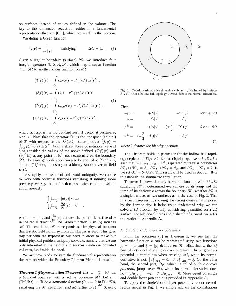
Fig. 2. Two-dimensional slice through a volume Ω2 (delimited by surfacesS1, S2) with a hollow ball topology. Arrows denote the normal orientation.

Then

−p = +N[u] −D∗[p] for r 6∈ ∂Ω

u = −D[u] +S[p]

−p± = +N[u] +(

± I

2− D

∗)

[p] for r ∈ ∂Ω

u± =(

∓ I

2− D

)

[u] +S[p]

(7)where I denotes the identity operator.

The Theorem holds in particular for the hollow ball topol-ogy depicted in Figure 2, i.e. for disjoint open sets Ω1,Ω2,Ω3

such that Ω1∪Ω2∪Ω3 = R3, separated by regular boundaries

∂Ω1 ∩ ∂Ω2 = S1, ∂Ω2 ∩ ∂Ω3 = S2, and ∂Ω1 ∩ ∂Ω3 = ∅, ifwe set ∂Ω = S1∪S2. This result will be used in Section III-Gto establish the symmetric formulation.

Theorem 1 shows that any harmonic function u in R3\∂Ω

satisfying H is determined everywhere by its jump and thejump of its derivative across the boundary ∂Ω, whether ∂Ω isa single surface, or two surfaces as in the case of Fig. 2. Thisis a very deep result, showing the strong constraints imposedby the harmonicity. It helps us to understand why we cansolve a 3D problem by only considering quantities on a 2Dsurface. For additional notes and a sketch of a proof, we referthe reader to Appendix A.

A. Single and double-layer potentials

From the equations (7) in Theorem 1, we see that theharmonic function u can be represented using two functionsµ = −[u] and ξ = [p] defined on ∂Ω. Historically, the Sξpart of (7) is called a single-layer potential. The single-layerpotential is continuous when crossing ∂Ω, while its normalderivative is not;

[

Sξ]

∂Ω= 0,

[

∂nSξ]

∂Ω= ξ. On the other

hand, the second part, Dµ, which is called a double-layerpotential, jumps over ∂Ω, while its normal derivative doesnot;

[

Dµ]

∂Ω= −µ,

[

∂nDµ]

∂Ω= 0. More detail on single

and double-layer potentials is provided in Appendix A.To apply the single/double-layer potentials to our nested-

region model in Fig. 1, we simply add up the contributions

4

from all interfaces, us =∑

i SξSiresp. ud =

∑

i DµSi. This

yields single, resp. double-layer potentials with the same jumpproperties as in the single interface case (see Appendix B). Inparticular, we shall need further on the following two relations,easily obtainable from (7) by additivity:

∂nu±s (r) = ∓ξSj

2+

N∑

i=1

D∗jiξSi

for r ∈ Sj (8)

u±d (r) = ±µSj

2+

N∑

i=1

DjiµSifor r ∈ Sj . (9)

The operators D∗ji and Dji are restrictions of D∗ and D: they

act on a function defined on Si and yield a function definedon Sj . This convention is used consistently in the rest of thispaper.

III. INTEGRAL FORMULATIONS

Let us use Theorem 1 to obtain integral formulations forthe original multiple interface problem (4). We now need tocope with the presence of sources, which make the solutionnon-harmonic. Our starting point is a homogeneous solutionv, which takes the source terms into account, but does notnecessarily respect all boundary conditions. Then we add to va harmonic function u to obtain a complete solution V whichsimultaneously respects the Poisson equation σi∆V = f in allΩi, the boundary conditions (4), and the equation (3). Threedifferent ways of achieving this are described in this section.We shall always assume that V satisfies condition H , whichamounts to imposing a zero potential infinitely far from allsources.

A. Dipolar and surface sources

The source model most commonly used to represent electri-cal activity in the brain is a “current dipole”1 [3]. It representsan infinitely small oriented source of current positioned at r0,with dipolar moment q, and is defined by Jdip(r) = q δr0

(r).The corresponding source term in the Poisson equation isfdip = ∇ · Jdip = q · ∇δr0

, which yields the homogeneousdomain potential

vdip(r) =1

4π

q · (r − r0)

‖r − r0‖3. (10)

The dipolar source is physiologically plausible in that it repre-sents movement of charges, not their creation. At sufficientlylong time scale it approximates the neuronal pulse trains.

Sources on cortex surface and perpendicular to it can bealso modeled as Jsurf(r) = j(r)nP (r) δP (r) with scalarsurface current density j on a patch P . The correspondinghomogeneous potential vsurf is then calculated by integrationover P :

vsurf(r) =1

4π

∫

r′∈P

nP (r′) · (r − r′)

‖r − r′‖3j(r′) dr′ (11)

Finally, we can consider a completely general volume currentdensity Jp, yielding a source term f = ∇ · Jp and a potentialv = −f ∗G. (See also next Section.)

1This is a traditional name, used because the quantity q has the units of[A · m].

B. Homogeneous solution

We decompose the source f from (1) into f =∑N

i=1 fΩi

such that fΩi= f · 1Ωi

, where 1Ωiis the indicator function

of Ωi (hence fΩi= 0 outside Ωi), i = 1, · · · , N . Recall that

no source lies in ΩN+1; we also assume that no source lieson any boundary Si.

For each partial source term fΩiwe calculate the homoge-

neous medium solution vΩi(r) = −fΩi

∗ G (r). The convo-lution theorem and the properties of the Green function (5)show that ∆vΩi

= −fΩi∗ ∆G = fΩi

. The vΩiare harmonic

in R\Ωi, i = 1, · · · , N and, hence also in ΩN+1. Thanks tothe choice of G in (5), the functions vΩi

satisfy condition H ,provided that the fΩi

are compactly supported. This is true byconstruction for Ω1, . . . ,ΩN since each of these domains isbounded.

C. Multiple domains

There are various ways of combining the individual ho-mogeneous solutions vΩi

from domains Ωi into a globalhomogeneous v. First we consider a function vs constructedas:

vs =

N∑

i=1

vΩi/σi . (12)

We easily verify that it satisfies the Poisson equation σ∆vs =f in each Ωi, i = 1, . . . , N :

σ∆vs = σN∑

i=1

∆vΩi/σi = σ

N∑

i=1

fΩi

σi

=N∑

i=1

fΩi= f

According to the previous section, all functions vΩi, i =

1, . . . , N are harmonic in ΩN+1, hence so is vs.The function vs and its derivative ∂nvs are continuous

across each Sj . In other words, vs satisfies the boundaryconditions

[

vs

]

j= 0 and

[

∂nvs

]

j= 0 for all j, but not the

boundary condition[

σ∂nvs

]

j= 0. The function vs will be

used in the single-layer approach, Section III-D, whence thesubscript s.

In a dual fashion, we would like to consider the functionvd(r) = σ−1(r)

∑Ni=1 vΩi

that satisfies σ∆vd = f and theboundary condition

[

σ∂nvd

]

j= 0. Unfortunately, vd is not

properly defined in ΩN+1 where σ = 0. Instead, we introducea function

vd =

N∑

i=1

vΩi(13)

that satisfies the Poisson equation ∆vd = f and the boundaryconditions

[

vd

]

j= 0 and

[

∂nvd

]

j= 0 on each surface Sj . The

function vd is harmonic in ΩN+1 for the same reasons as vs.This function is used in the double-layer approach, Section III-E.

D. Single-layer approach

A natural approach for solving (1) consists in representingthe potential V in a way which automatically satisfies [V ]j = 0and then adjusting the harmonic part so that the remainingboundary conditions, [σ∂nV ]j = 0, are satisfied as well. We

5

consider us = V −vs, with vs defined in (12). By construction,us is harmonic in Ω = Ω1 ∪ . . . ∪ ΩN , since in each Ωi wehave σi∆us = σi∆V − σi∆vs = fΩi

− fΩi= 0. It is also

harmonic in ΩN+1, as both V and vs are harmonic there.Since [V ]j = 0 and [vs]j = 0 (Section III-C), we concludethat [us]j = 0 across all surfaces Sj . This means that us isa single-layer potential for Ω = Ω1 ∪ . . . ∪ ΩN+1 with thecorresponding boundary ∂Ω = S1 ∪ . . . ∪ SN ( cf Section II-A).

We then use the second set of boundary conditions,[σ∂nV ] = 0, implying that [σ∂nus] = −[σ∂nvs]. We express[σ∂nus] as a function of known quantities:[

σ∂nus

]

j= −

[

σ∂nvs

]

j= −(σj − σj+1)∂nvs on Sj (14)

since ∂nvs does not “jump” across Sj (Section III-C). Equa-tion (8) provides the normal derivative of the single-layerpotential us. Writing ξSj

=[

∂nus

]

j,

[

σ∂nus

]

j= σj∂nu

−s − σj+1∂nu

+s =

σj + σj+1

2ξSj

+ (σj − σj+1)

N∑

i=1

D∗jiξSi

on all S1, . . . , SN . Combining this result with (14) and divid-ing by (σj − σj+1) we obtain2

∂nvs =σj + σj+1

2(σj+1 − σj)ξSj

−N∑

i=1

D∗jiξSi

on all Sj . (15)

This is a system of N integral equations in the unknownfunctions ξSj

. Its solution is unique up to a constant [7] (seealso Appendix C). Once (15) is solved, the potential us isdetermined for r ∈ Sj as

us(r) =

N∑

i=1

SjiξSi,

and the corresponding values of V follow from V = vs + us.We observe that V is expressed as an exactly calculable

homogeneous medium potential vs plus a correction term us.If the medium is close to homogeneous, the correction is small,which helps to improve the accuracy of this method. Thismethod is to be favored if we are interested in calculating theflow or the current. However, to obtain the potential V , anadditional computation is necessary.

E. Double-layer approach

The double-layer approach is dual to the single-layer ap-proach. We use a representation satisfying [σ∂nV ]j = 0 byconstruction and then find conditions on the harmonic part toimpose [V ]j = 0 as well. Consider a function ud = σV − vd,with vd given by (13). By construction, ud is harmonic inΩ = Ω1 ∪ . . . ∪ ΩN , because in each Ωi we have ∆ud =σi∆V −∆vd = fΩi

− fΩi= 0. It is also harmonic in ΩN+1,

as both V and vd are harmonic there. Since [σ∂nV ]j = 0 and[∂nvd]j = 0 (Section III-C), we conclude that [∂nud]j = 0

2The division by (σj − σj+1) has been done to simplify the formula.It should not be performed for small values |σj − σj+1| in order to avoidnumerical difficulties.

on all surfaces Sj . This means that ud is a double-layerpotential for Ω = Ω1 ∪ . . . ∪ ΩN+1 with the correspondingboundary ∂Ω = S1 ∪ . . . ∪ SN . Equation (9) expresses theboundary values of a double-layer representation. We now usethe second set of boundary conditions, [V ]j = 0, implyingthat σj+1(ud + vd)

− = σj(ud + vd)+ for all Sj . (This is

equivalent to σ−1j (ud + vd)

− = σ−1j+1(ud + vd)

+ for σ 6= 0and a natural extension thereof for σ = 0.) We can also expressµSi

= −[ud] = (σi+1 − σi)VSi, where VSi

is the restrictionof V to Si. This yields

vd =σj + σj+1

2VSj

−N∑

i=1

(σi+1 − σi)DjiVSion each Sj .

(16)The function vd defined in (13) is the solution of∆vd = f , corresponding to a homogeneous mediumwith conductivity equal to one. Remembering thatDjiVSi

(r) =∫

Si∂n′G(r − r′)V (r′) ds(r′) for r ∈ Sj ,

we recognize in (16) the classical integral formulation usedfor EEG and MEG [2, 3, 17, 19, 20]. The advantage of thisapproach is that it solves directly for V and requires noadditional post-processing. As in the single-layer approach,the solution of the system (16) is unique up to a constant [7].

F. Isolated problem approach

In 1989, Hamalainen and Sarvas [13] introduced a variationon this double-layer formulation, to improve the precision ofthe the classical formulation, caused by the low conductivityof the skull compared to the other head tissues. This approach,called Isolated Problem Approach (IPA) or Isolated Skull Ap-proach, is based on the same idea that improves the accuracyof the single-layer method — we express the potential V asa sum of two parts calculated separately with hopefully moreprecision than calculating the final result directly. In this case,we calculate first the field of the sources considering only theinnermost volume and then the appropriate correction.

The IPA is not general in that it assumes the sources tobe only in the innermost layer, which is not the case for themore realistic models of the head, where we want to considersources in the cortex. Also, while it improves the precision insome cases, it reduces it in others [20]. Therefore, we shallnot consider IPA in the rest of this article.

G. Symmetric approach

The symmetric approach, uses both the single and double-layer potentials. It is based on the classical theory of Newto-nian potentials as described in chapter 2 of [26], the work ofNedelec [7] and is also closely related to algorithms in [23,24]. However, as far as we know, it has so far never beendescribed for the EEG problem. In this approach, we considerin each Ω1, . . . ,ΩN the function

uΩi=

V − vΩi/σi in Ωi

−vΩi/σi in R

3\Ωi .

Each uΩiis harmonic in R

3\∂Ωi. Considering the nestedvolume model (Fig. 1), the boundary of Ωi is ∂Ωi = Si−1∪Si.

61

Ωi Ωi+1

Si Si+1Si−1

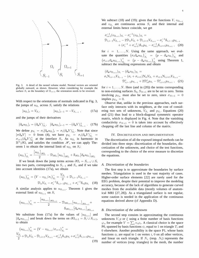
Fig. 3. A detail of the nested volume model. Normal vectors are orientedglobally outward, as shown. However, when considering for example thesurface Si as the boundary of Ωi+1, the orientation needs to be reversed.

With respect to the orientations of normals indicated in Fig. 3,the jumps of uΩi

across Si satisfy the relations

[uΩi]i = VSi

, [uΩi]i−1 = −VSi−1

, (17a)

and the jumps of their derivatives

[∂nuΩi]i = (∂nV )−Si

, [∂nuΩi]i−1 = −(∂nV )+Si−1

. (17b)

We define pSi= σi[∂nuΩi

]i = σi(∂nV )−Si. Note that since

[σ∂nV ] = 0 from (4), we have pSi= σi(∂nV )−Si

=

σi+1(∂nV )+Siat the interface Si. As uΩi

is harmonic inR

3\∂Ωi and satisfies the condition H , we can apply The-orem 1 to obtain the internal limit of uΩi

on Si:

(

uΩi

)−

Si=

[

uΩi

]

∂Ωi

2− D∂Ωi

[

uΩi

]

∂Ωi+ S∂Ωi

[

∂nuΩi

]

∂Ωi

If we break down the jump terms across ∂Ωi = Si−1 ∪ Si

into two parts, corresponding to Si−1 and Si, and if we takeinto account identities (17a), we obtain

(

uΩi

)−

Si=(

V − vΩi/σi

)−

Si=VSi

2+ Di,i−1VSi−1

−DiiVSi

− σ−1i Si,i−1pSi−1

+ σ−1i SiipSi

(18)

A similar analysis applies to uΩi+1. Theorem 1 gives the

external limit of uΩi+1on Si

(

uΩi+1

)+

Si= −

[

uΩi+1

]

∂Ωi+1

2− D∂Ωi+1

[

uΩi+1

]

∂Ωi+1+

S∂Ωi+1

[

∂nuΩi+1

]

∂Ωi+1

We substitute from (17a) for the values of [uΩi+1] and

[∂nuΩi+1] and break down the terms on ∂Ωi+1 = Si ∪ Si+1,

to obtain(

uΩi+1

)+

Si=(

V − vΩi+1/σi+1

)+

Si=

VSi

2+DiiVSi

−Di,i+1VSi+1−σ−1

i+1SiipSi+σ−1

i+1Si,i+1pSi+1

(19)

We subtract (18) and (19); given that the functions V, vΩi+1

and vΩiare continuous across Si and their internal and

external limits hence coincide, we get

σ−1i+1(vΩi+1

)Si− σ−1

i (vΩi)Si

=

Di,i−1VSi−1− 2DiiVSi

+ Di,i+1VSi+1− σ−1

i Si,i−1pSi−1

+ (σ−1i + σ−1

i+1)SiipSi− σ−1

i+1Si,i+1pSi+1, (20)

for i = 1, . . . , N . Using the same approach, we eval-uate the quantities

(

σi∂nuΩi

)−

Si=

(

p − ∂nvΩi

)−

Siand

(

σi+1∂nuΩi+1

)+

Si=

(

p − ∂nvΩi+1

)+

Siusing Theorem 1,

subtract the resulting expressions and obtain

(∂nvΩi+1)Si

− (∂nvΩi)Si

=

σiNi,i−1VSi−1− (σi + σi+1)NiiVSi

+ σi+1Ni,i+1VSi+1−

D∗i,i−1pSi−1

+ 2D∗iipSi

− D∗i,i+1pSi+1

, (21)

for i = 1, . . . , N . Here (and in (20)) the terms correspondingto non-existing surfaces S0, SN+1 are to be set to zero. Termsinvolving pSN

must also be set to zero, since σN+1 = 0implies pSN

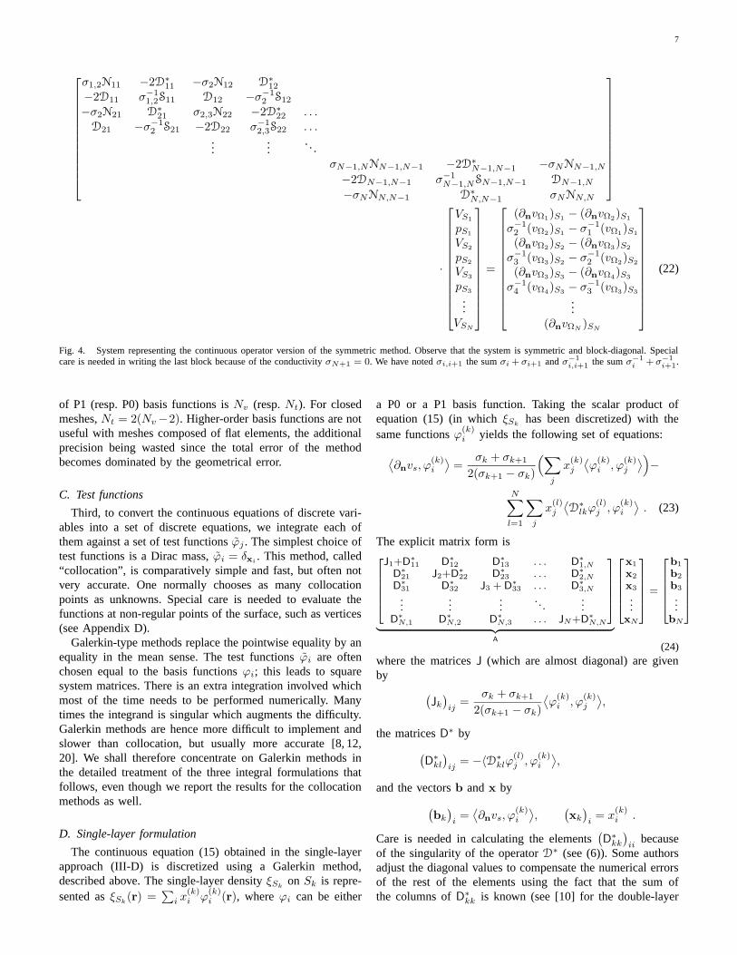
= 0.Observe that, unlike in the previous approaches, each sur-

face only interacts with its neighbors, at the cost of consid-ering two sets of unknowns, VSi

and pSi. Equations (20)

and (21) thus lead to a block-diagonal symmetric operatormatrix, which is displayed in Fig. 4. Note that the vanishingconductivity σN+1 = 0 is taken into account by effectivelychopping off the last line and column of the matrix.

IV. DISCRETIZATION AND IMPLEMENTATION

The discretization of all the exposed integral methods can bedivided into three steps: discretization of the boundaries, dis-cretization of the unknowns, and choice of the test functions,corresponding to the choice of the error measure to discretizethe equations.

A. Discretization of the boundaries

The first step is to approximate the boundaries by surfacemeshes. Triangulation is used in the vast majority of cases.Higher-order surface elements [22] are rarely used for theEEG problem, despite their potential to improve the modelingaccuracy, because of the lack of algorithms to generate curvedmeshes from the available data (mostly volumes of anatom-ical MRI [27, 28]). As a triangulated surface is not regular,some caution is needed in the application of the continuousequations derived above (cf Appendix D).

B. Discretization of the unknowns

The second step consists in approximating the continuousunknowns V, p or ξ using a finite number of basis functionsϕi, for example V =

∑

i viϕi. A classical choice is the spaceP0, spanned by basis functions ψi equal to 1 on triangle Ti and0 elsewhere. Another possibility is the space P1, whose basisfunctions φi are equal to 1 on vertex i, 0 on all other vertices,and linear on each triangle. If Nv (resp. Nt) represents thenumber of vertices (resp. triangles) in the mesh, the number

7

σ1,2N11 −2D∗11 −σ2N12 D∗

12

−2D11 σ−11,2S11 D12 −σ−1

2 S12

−σ2N21 D∗21 σ2,3N22 −2D∗

22 . . .D21 −σ−1

2 S21 −2D22 σ−12,3S22 . . .

......

. . .σN−1,NNN−1,N−1 −2D∗

N−1,N−1 −σNNN−1,N

−2DN−1,N−1 σ−1N−1,NSN−1,N−1 DN−1,N

−σNNN,N−1 D∗N,N−1 σNNN,N

·

VS1

pS1

VS2

pS2

VS3

pS3

...VSN

=

(∂nvΩ1)S1

− (∂nvΩ2)S1

σ−12 (vΩ2

)S1− σ−1

1 (vΩ1)S1

(∂nvΩ2)S2

− (∂nvΩ3)S2

σ−13 (vΩ3

)S2− σ−1

2 (vΩ2)S2

(∂nvΩ3)S3

− (∂nvΩ4)S3

σ−14 (vΩ4

)S3− σ−1

3 (vΩ3)S3

...(∂nvΩN

)SN

(22)

Fig. 4. System representing the continuous operator version of the symmetric method. Observe that the system is symmetric and block-diagonal. Specialcare is needed in writing the last block because of the conductivity σN+1 = 0. We have noted σi,i+1 the sum σi + σi+1 and σ−1

i,i+1 the sum σ−1i + σ−1

i+1.

of P1 (resp. P0) basis functions is Nv (resp. Nt). For closedmeshes, Nt = 2(Nv −2). Higher-order basis functions are notuseful with meshes composed of flat elements, the additionalprecision being wasted since the total error of the methodbecomes dominated by the geometrical error.

C. Test functions

Third, to convert the continuous equations of discrete vari-ables into a set of discrete equations, we integrate each ofthem against a set of test functions ϕj . The simplest choice oftest functions is a Dirac mass, ϕi = δxi

. This method, called“collocation”, is comparatively simple and fast, but often notvery accurate. One normally chooses as many collocationpoints as unknowns. Special care is needed to evaluate thefunctions at non-regular points of the surface, such as vertices(see Appendix D).

Galerkin-type methods replace the pointwise equality by anequality in the mean sense. The test functions ϕi are oftenchosen equal to the basis functions ϕi; this leads to squaresystem matrices. There is an extra integration involved whichmost of the time needs to be performed numerically. Manytimes the integrand is singular which augments the difficulty.Galerkin methods are hence more difficult to implement andslower than collocation, but usually more accurate [8, 12,20]. We shall therefore concentrate on Galerkin methods inthe detailed treatment of the three integral formulations thatfollows, even though we report the results for the collocationmethods as well.

D. Single-layer formulation

The continuous equation (15) obtained in the single-layerapproach (III-D) is discretized using a Galerkin method,described above. The single-layer density ξSk

on Sk is repre-sented as ξSk

(r) =∑

i x(k)i ϕ

(k)i (r), where ϕi can be either

a P0 or a P1 basis function. Taking the scalar product ofequation (15) (in which ξSk

has been discretized) with thesame functions ϕ(k)

i yields the following set of equations:

⟨

∂nvs, ϕ(k)i

⟩

=σk + σk+1

2(σk+1 − σk)

(

∑

j

x(k)j

⟨

ϕ(k)i , ϕ

(k)j

⟩

)

−

N∑

l=1

∑

j

x(l)j

⟨

D∗lkϕ

(l)j , ϕ

(k)i

⟩

. (23)

The explicit matrix form is2

66664

J1+D∗11 D

∗12 D

∗13 . . . D

∗1,N

D∗21 J2+D

∗22 D

∗23 . . . D

∗2,N

D∗31 D

∗32 J3 + D

∗33 . . . D

∗3,N

......

.... . .

...D

∗N,1 D

∗N,2 D

∗N,3 . . . JN+D

∗N,N

3

77775

| z

A

2

66664

x1

x2

x3

...xN

3

77775

=

2

66664

b1

b2

b3

...bN

3

77775

(24)where the matrices J (which are almost diagonal) are givenby

(

Jk

)

ij=

σk + σk+1

2(σk+1 − σk)

⟨

ϕ(k)i , ϕ

(k)j

⟩

,

the matrices D∗ by

(

D∗kl

)

ij= −〈D∗

klϕ(l)j , ϕ

(k)i

⟩

,

and the vectors b and x by

(

bk

)

i=⟨

∂nvs, ϕ(k)i

⟩

,(

xk

)

i= x

(k)i .

Care is needed in calculating the elements(

D∗kk

)

iibecause

of the singularity of the operator D∗ (see (6)). Some authorsadjust the diagonal values to compensate the numerical errorsof the rest of the elements using the fact that the sum ofthe columns of D∗

kk is known (see [10] for the double-layer

8

approach). This arises from the fact that the total solid angleω = 4π

(

Di1)

(r) must be equal to 4π for all interior points,and from the physical necessity of obtaining a singular matrix(see Appendix C). The notation Di indicates that the operatorD is restricted to the ith interface. However, we prefer to set(

D∗kk

)

iito 0, which is exact at regular points of flat surfaces

(triangles), trivial to compute, and unlike the former approachdoes not obscure potential accuracy problems. We did notobserve a significant difference in accuracy between the twochoices.

The system matrix A is full and non-symmetric. Theelements of the matrices D∗ involve double integrals overtriangles of the meshes. The inner integrals can be calculatedanalytically for both P0 and P1 basis functions [19, 29, 30];the outer integrals must be calculated numerically, which ismost efficiently done using a Gaussian quadrature adapted totriangles [6, 31].

Once x is known, the potential V is calculated directlyfrom (III-D) as

V (r) = vs(r) +

N−1∑

l=1

∑

j

x(l)j

(

Slkϕ(l)j

)

(r) for r ∈ Sk .

(25)Note that no approximation is involved here; if x is knownexactly, V can be calculated exactly too.

E. Deflation

An important point to note is that the matrix A presentedin (24) is singular (see Appendix C). We “deflate” it [32]using the condition 〈ξ, 1〉 = 0 (see Appendix C). For thecommonly used basis functions satisfying the partition of unityproperty3, this is equivalent to

∑

i x(k)i = 0 on each Sk,

and thus∑

ik x(k)i = 0. To impose this, we replace A with

A′ = A + ω11T , where ω is chosen such that A′ is wellconditioned. The optimal choice of ω is too costly to calculatebut the value is not very critical and can be approximated [12,33]. We use the fact that A is approximately diagonal dominantand we assume that the very first element is representative,which leads to ω =

(

A)

11/M , where M is the total number

of unknowns. This was found to perform acceptably well. Thedeflated matrix A′ is regular and square and can be invertedby the usual methods.

Note that deflation is not equivalent to regularization thatlooks for a smooth solution only approximately satisfying theMaxwell equations. Instead, deflation chooses one solutionfrom a family of equivalent ones, all satisfying the equationsexactly, according to our preferences based on the physics ofthe problem.

F. Double-layer formulation

The double-layer formulation (16) is discretized using thesame approach as the single-layer one, with VSk

on Sk

represented as VSk(r) =

∑

i x(k)i ϕ

(k)i (r), where ϕi is either

3Their sum is equal to 1 everywhere.

P0 or P1. Taking the scalar product of (16) with ϕ(k)i yields

⟨

vd, ϕ(k)i

⟩

=σk + σk+1

2

(

∑

j

x(k)j

⟨

ϕ(k)i , ϕ

(k)j

⟩

)

−

N∑

l=1

(σl+1 − σl)∑

j

x(l)j

⟨

Dklϕ(l)j , ϕ

(k)i

⟩

(26)

or, in a matrix form

2

66664

J1+D11 D12 D13 . . . D1,N

D21 J2+D22 D23 . . . D2,N

D31 D32 J3+D33 . . . D3,N

......

.... . .

...DN,1 DN,2 DN,3 . . . JN+DN,N

3

77775

| z

A

x1

x2

x3

...xN

=

b1

b2

b3

. . .bN

(27)

where

(

Jk

)

ij=σk + σk+1

2

⟨

ϕ(k)i , ϕ

(l)j

⟩

(

Dkl

)

ij= −(σl+1 − σl)〈Dklϕ

(l)j , ϕ

(k)i

⟩

(

bk

)

i=⟨

vd, ϕ(l)i

⟩

,(

xk

)

i= x

(k)i

As in the single-layer case, and thanks to the duality betweenD and D∗, the inner integrals needed to calculate elementsof matrices Dlk have an analytical solution for both P0 andP1 basis functions [19, 29], while the outer integrals arecalculated numerically [8]. The matrix is again full, non-symmetric, and needs to be deflated, this time because thepotential V is only defined up to a constant (see Appendix C).Imposing the condition H is impractical, and we insteadimpose either the mean of the potential over all surfaces tobe zero,

∑Nk=1

∑

i x(k)i = 0, or else the mean of the potential

over the external surface to be zero,∑

i x(N)i = 0. In the

latter case we propose to modify (deflate) only the bottom-right block of A, namely JN + DN,N . The basis functions areassumed to satisfy the partition of unity property.

The continuous V is directly accessible from the discretiza-tion equation V (r) =

∑

i x(k)i ϕ

(k)i for r ∈ Sk.

G. Symmetric approach

The specificity of the discretization of the symmetric ap-proach (20,21) is that both V and its derivative p are simul-taneously involved as unknowns. The approximation errorsfor the two quantities should be asymptotically equivalent,so that the overall error is not dominated by either one.For this reason, we choose to approximate V using P1 basisfunctions as VSk

(r) =∑

i x(k)i φ

(k)i (r), while its derivative p

is represented using the space P0, pSk(r) =

∑

i y(k)i ψ

(k)i (r).

Similar concerns guide our choice of test functions. We noticethat the operator S behaves as a smoother: it increases theregularity of its argument [7] by one. The operators D, D∗ donot change it, while N has a derivative character: it decreasesthe regularity by one. The regularity is closely tied to anapproximation order [34]. To balance the errors, all the scalarproducts should have the same approximation order. To ensure

9

this, we multiply (20) concerning the potential (a P1 function)by P0 test functions ψi

⟨

σ−1k+1vΩk+1

− σ−1k vΩk

, ψ(k)i

⟩

=∑

j

x(k−1)j

⟨

Dk,k−1φ(k−1)j , ψ

(k)i

⟩

+

∑

j

x(k+1)j

⟨

Dk,k+1φ(k+1)j , ψ

(k)i

⟩

+ (σ−1k + σ−1

k+1)∑

j

y(k)j

⟨

Skkψ(k)j , ψ

(k)i

⟩

− σ−1k

∑

j

y(k−1)j

⟨

Sk,k−1ψ(k−1)j , ψ

(k)i

⟩

− σ−1k+1

∑

j

y(k+1)j

⟨

Sk,k+1ψ(k+1)j , ψ

(k)i

⟩

− 2∑

j

x(k)j

⟨

Dkkφ(k)j , ψ

(k)i

⟩

,

and (21) concerning the flow (a P0 function) by P1 testfunctions φi

⟨

∂nvΩk+1− ∂nvΩk

, φ(k)i

⟩

=

σk

∑

j

x(k−1)j

⟨

Nk,k−1φ(k−1)j , φ

(k)i

⟩

+ σk+1

∑

j

x(k+1)j

⟨

Nk,k+1φ(k+1)j , φ

(k)i

⟩

− (σk + σk+1)∑

j

x(k)j

⟨

Nkkφ(k)j , φ

(k)i

⟩

−∑

j

y(k−1)j

⟨

D∗k,k−1ψ

(k−1)j , φ

(k)i

⟩

−∑

j

y(k+1)j

⟨

D∗k,k+1ψ

(k+1)j , φ

(k)i

⟩

+ 2∑

j

y(k)j

⟨

D∗kkψ

(k)j , φ

(k)i

⟩

,

both to hold on all interfaces k = 1, . . . , N . This set ofequations can be expressed more concisely in matrix formThe matrix A should be truncated4 like in (22), to account forthe zero conductivity σN+1 = 0.

Note that A is larger than in the single or double-layer cases.However, it is symmetric and block-diagonal, which meansthat the actual number of elements to be stored is comparableor even smaller, depending on the number of interfaces. More-over, matrices Nkl can be calculated at negligible costs fromthe intermediate results needed for calculating matrices Skl,thanks to an interesting relation coming from Theorem 3.3.2in [7]:⟨

Nklϕ′i, ϕ

′j

⟩

= −(qi × ni)(qj × nj)⟨

Sklψ(l)j , ψ

(k)i

⟩

(29)

where ϕ′i(x) =

(

qi · x + αi

)

ψi(x) and ϕ′j(x) =

(

qj ·x + αj

)

ψj(x) are the P1 basis functions ϕ restricted to onetriangle.

Deflation is needed to avoid the indetermination of V .To impose a zero mean of the potential on the outermostsurface, only the bottom-right block with NN,N is modified

4The bottom-right corner of A is not shown here for space reasons.

TABLE I

THE DIFFERENT METHODS IMPLEMENTED AND THEIR ASSOCIATED

LABELS.

Label Formulation ϕ ψ

1a Single-Layer P0 Dirac1b P0 P01c P1 P12a Double-Layer P0 Dirac2b P0 P02c P1 P13 Symmetric P0 P1

to NN,N + ω11T , using the heuristic ω =(

NN,N

)

11/MN , as

in Section IV-E.

H. Acceleration

As the number of mesh elements M grows, the matrixassembly time O(M2) becomes dominated by the time neededto solve the resulting linear system O(M 3), e.g. by theLU decomposition. Iterative solvers [8, 9, 35] can be usedinstead, reducing the computation time and only accessing thematrix by matrix-vector multiplications Az. This brings otheroptimization opportunities such as calculating these productsapproximately using a fast multipole method (FMM) [11],precorrected-FFT [14, 36] or SVD-based methods. Multires-olution techniques permit to reduce the number of expensiveiterations on the finest level by solving first a reduced sizeproblem and using its solution as the starting guess. Multigridalgorithms combine iterations on fine and coarse levels foreven faster convergence.

Parallelizing the assembly phase is straightforward as thematrix elements can be calculated independently, even thoughfor optimum performance the expensive calculations neededto calculate S should be reused for the calculation of N,as mentioned above. Parallel techniques also exist for linearsystem solver non-iterative algorithms (SCALAPACK library).

V. EXPERIMENTS

We have implemented the single-layer, double-layer, andsymmetric approaches described in this article in both serialand parallel versions. The single and double-layer approachesexist in three discretization variants: with the collocationmethod (ϕj = δxj

) using the P0 basis functions ϕ, and withthe Galerkin method (ϕj = ϕj) using both P0 and P1 bases.The symmetric method is discretized using P1 basis functionsfor V and P0 basis functions for p. We have implementedonly this choice, since with other discretizations we lose theprincipal advantages of the method, symmetry and accuracy.We have applied these methods first to synthetic cases wherean analytical solution is known, as well as to realisticallyshaped head models.

Table I summarizes the different discretization choices, andindicates the labels by which they are referenced in the textand figures.

10

2

666666664

(σ1+σ2)N11 −2D∗11 −σ2N12 D

∗12

−2D11 (σ−11

+σ−12

)S11 D12 −σ−12

S12

−σ2N21 D∗21 (σ2+σ3)N22 −2D∗

22 −σ3N23 D∗23

D21 −σ−12

S21 −2D22 (σ−12

+σ−13

)S22 D23 −σ−13

S23

−σ3N32 D∗32 (σ3+σ4)N33 −2D∗

33 . . .D32 −σ

−13

S32 −2D33 (σ−13

+σ−14

)S33 . . ....

.... . .

3

777777775

| z

A

2

666666664

x1

y1

x2

y2

x3

y3

...

3

777777775

| z

w

=

2

666666664

b1

c1

b2

c2

b3

c3

...

3

777777775

| z

z

(28)

with(

Nkl)ij =⟨

Nklφ(l)j , φ

(k)i

⟩ (

Skl)ij =⟨

Sklψ(l)j , ψ

(k)i

⟩

(

Dkl)ij =(

D∗lk)ji =

⟨

Dklφ(l)j , ψ

(k)i

⟩

(

bk

)

i=⟨

∂nvΩk− ∂nvΩk+1

, φ(k)i

⟩

(

ck

)

i=⟨

σ−1k+1vΩk+1

− σ−1k vΩk

, ψ(k)i

⟩

(

xk

)

i= x

(k)i

(

yk

)

i= y

(k)i

A. Speed

The speed depends strongly on the desired precision, onthe optimization and acceleration techniques applied and onthe specific task.5 In our experiments, the time needed forthe direct assembly of the matrix was of the order of 1 to5 s for our smallest head mesh of 3 × 42 vertices, to severalminutes to assemble the matrices of 4486 × 4486 elements,corresponding to the meshes of 3 × 642 vertices, up to about2 h for the matrices of 17926×17926, corresponding to meshesof 3 × 2562 vertices. Using a parallel code on a clusterof workstations speeds the assembling proportionally to thenumber of processors with a high efficiency. The time neededto solve the linear system of equations varied between 10 msand 2 h for the same cases. Generally, the assembly time growsquadratically with the number of degrees of freedom, and thesolution time as a third power. Collocation methods can be10 or more times faster than the Galerkin method, dependingon the numerical integration method used and the number ofintegration points needed to get the required accuracy. Thesingle-layer method is more costly than the correspondingdouble-layer method6, as two matrices need to be assembled,the matrix A in (24) in order to solve for the single-layerdensity, and an additional matrix in order to integrate thepotential from equation (25).

B. Spherical head models

The first part of our tests was performed on triangulatedspherical surfaces. The choice of a spherical geometry hasthe advantage that an analytical solution is available [20, 37,38], thus making it possible to evaluate the accuracy of thedifferent methods. The spherical surfaces were triangulatedwith progressively finer meshes of 42, 162, and 642 verticesper layer7. We used three concentric spheres with radii 0.87,

5For example, one may consider that the system matrix, once assembled,can be used to solve many problems involving the same geometry. This makesthe actual assembly time irrelevant.

6The precise ratio depends on the discretization used.7Finer meshes were avoided in this set of experiments because of memory

and time limitations so that a serial direct solver could be used for mostreproducible results.

0.92, and 1.0, delimiting volumes with conductivities 1.0,0.0125, 1.0 and 0.0, from inside towards outside. The sourceswere unitary current dipoles oriented as [1 0 1]/

√2 and placed

at distances r = 0.425, 0.68, 0.765, 0.8075, and 0.8415 fromthe center on the x axis.

We chose to evaluate the analytical solution at trianglecenters for the P0 methods and at vertex points for theothers. This disadvantages Galerkin methods but it is closeto actual use. We then calculated the relative `2 error ‖vanal −vnum‖`2/‖vanal‖`2 , making sure that both vanal and vnum hadzero means prior to comparison. Note that some authorslinearly scale vnum to obtain the best fit [10]. This obviouslysignificantly reduces the reported error but is difficult to justifyin the context of evaluating the accuracy of a method.

We have also made some experiments using a single spheremodel, not shown here because of lack of space and becauseit does not correspond to a plausible head model. Note that inthis case the symmetric model is disadvantaged by using onlythe operator N.

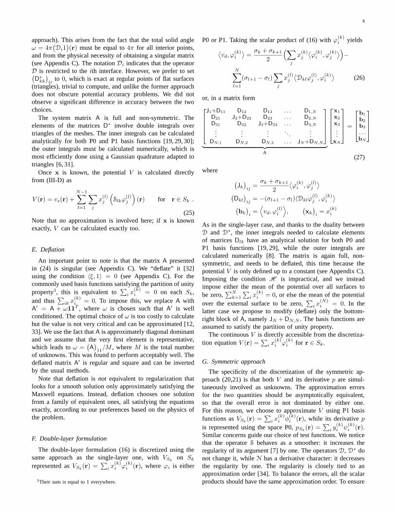
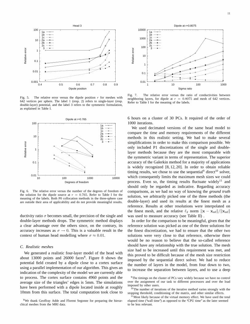
1) Error versus dipole position: The first set of experiments(Fig. 5) shows how the accuracy decreases when the currentdipole source approaches the surface of discontinuity. Weobserve that the symmetric approach is much less affectedthan the other methods.

2) Error versus mesh density: For a fixed source position(r = 0.765), the error decreases as the mesh is refined(Fig. 6). We observe that while both collocation variantsproduce the largest errors (results are completely unreliable),Galerkin methods based on P0 approximations are better, andthe best results are provided by the P1 methods, namely by thesymmetric formulation. Moreover, the slope of the decreaseof the error with mesh size is steeper for P1-based methods,a benefit of their higher approximation order.

3) Error versus conductivity: The accuracy of all im-plemented methods depends on the ratio of conductivitiesbetween the second layer (representing the skull) and theneighboring volumes (representing brain and scalp). To displaythis behavior, we have created additional head models withconductivities of the three volumes 1.0, σ, 1.0, with σ rangingbetween 1/2 and 1/1000. Figure 7 shows that when the con-

11

0.001

0.01

0.1

1

10

100

0.4 0.5 0.6 0.7 0.8 0.9

Rel

ativ

e er

ror

Dipole position

Head 3

1a1b1c2a2b2c3

Fig. 5. The relative error versus the dipole position r for meshes with642 vertices per sphere. The label 1 (resp. 2) refers to single-layer (resp.double-layer) potential, and the label 3 refers to the symmetric formulation,as explained in Table I.

0.01

0.1

1

10

100

10 100 1000 10000

Rel

ativ

e er

ror

Degrees of freedom

Dipole at r=0.765

1a1b1c2a2b2c3

Fig. 6. The relative error versus the number of the degrees of freedom ofthe solution for the dipole source at r = 0.765. Refer to Table I for themeaning of the labels. Both P0 collocation methods in the three-sphere caseare outside their area of applicability and do not provide meaningful results.

ductivity ratio σ becomes small, the precision of the single anddouble-layer methods drops. The symmetric method displaysa clear advantage over the others since, on the contrary, itsaccuracy increases as σ → 0. This is a valuable result in thecontext of human head modelling where σ ≈ 0.01.

C. Realistic meshes

We generated a realistic four-layer model of the head withabout 13000 points and 26000 faces8. Figure 8 shows thepotential field created by a dipole close to a cortex surfaceusing a parallel implementation of our algorithm. This gives anindication of the complexity of the model we are currently ableto process. The cortex surface contains 4960 points and theaverage size of the triangles’ edges is 5mm. The simulationshave been performed with a dipole located inside at roughly10mm from this surface. The total computation took close to

8We thank Geoffray Adde and Florent Segonne for preparing the hierar-chical meshes from the MRI data.

0.01

0.1

1

10

100

1000

10000

1 10 100 1000

Rel

ativ

e er

ror

Sigma ratio

Dipole at r=0.8075

1a1b1c2a2b2c3

Fig. 7. The relative error versus the ratio of conductivities betweenneighboring layers, for dipole at r = 0.8075 and mesh of 642 vertices.Refer to Table I for the meaning of the labels.

6 hours on a cluster of 30 PCs. It required of the order of1000 iterations.

We used decimated versions of the same head model tocompare the time and memory requirements of the differentmethods in this realistic setting. We had to make severalsimplifications in order to make this comparison possible. Weonly included P1 discretizations of the single and double-layer methods because they are the most comparable withthe symmetric variant in terms of representation. The superioraccuracy of the Galerkin method for a majority of applicationsis widely recognized [8, 12, 20]. In order to obtain reliabletiming results, we chose to use the sequential9 direct10 solver,which consequently limits the maximum mesh sizes we couldprocess. Even so, the timing results fluctuate widely11 andshould only be regarded as indicative. Regarding accuracycomparisons, as we had no way of knowing the ground truthsolution, we arbitrarily picked one of the three methods (thedouble-layer) and used its results at the finest mesh as areference. Results at other resolutions were interpolated onthe finest mesh, and the relative `2 norm ‖x − xref‖/‖xref‖was used to measure accuracy (see Table II) .

In order for the comparison to be meaningful, given that thereference solution was picked as one of the three solutions forthe finest discretization, we had to ensure that the other twosolutions were very close to that reference, otherwise therewould be no reason to believe that the so-called referenceshould have any relationship with the true solution. The meshsize had to be increased until this requirement was met, andthis proved to be difficult because of the mesh size restrictionimposed by the sequential direct solver. We had to reducethe number of layers in the model, from four down to two,to increase the separation between layers, and to use a deep

9The timings on the cluster of PCs vary widely because we have no controlover the assignment of our task to different processors and over the loadimposed by other users.

10The number of iterations of the iterative method varies strongly with thestopping threshold, conditioning of the matrix, and other similar effects.

11Most likely because of the virtual memory effect. We have used the totalelapsed time (“wall time”) as opposed to the “CPU time” as the later seemedto be less relevant.

12

dipole. At convergence, the results obtained by the threemethods differed in relative `2 norm by roughly 0.05 (5%)for the two-layer model.

We also ran computations on a three-layer model, but inthat case, the relative errors between results at the finestdiscretization were as high as 20%. It would have requiredeven finer meshes to achieve the same relative accuracy asin the two-layer case and it was not possible for the reasonsindicated above. This is the reason why the accuracy resultsin Table II (bottom) compare each method to its own result atthe finest discretization.

D. Discussion

A meaningful comparison of the various techniques isdifficult. First, one must bear in mind that they use differentnumber of degrees of freedom to perform the calculations,which moreover is not necessarily identical to the numberof degrees of freedom used to express the solution. Morespecifically, for a (closed) mesh with Nv vertices, P1 methodsinvolve Nv unknowns, P0 based methods use about 2Nv ofthem, while the symmetric method with P0/P1 discretizationuses about 3Nv unknowns, but only Nv degrees of freedomto express the solution V .

In the case of the spherical models with three layers wherethe ground truth is known analytically, Fig. 5 shows thatfor a dipole far from an interface, the single-layer methodperforms best. This probably comes from the fact that itrepresents the solution as an exact term plus a correction.When the dipole moves closer to the interface, the symmetricmethod yields the best results. Fig. 6 shows that the symmetricmethod is less sensitive than the single-layer and the double-layer method to a decrease in the quality of the descriptionof the geometry. Finally, Fig. 7 indicates that when theratio of conductivities between neighboring layers is betweenroughly 2 and 10 the single-layer method performs best,followed by the symmetric and the traditional double-layermethods, while when this ratio grows larger than 15, the newsymmetric method is clearly ahead of the single- and double-layer methods.

As stated above, in the case of the much more realisticmodel of Fig. 8 the comparison between the methods is moredifficult since the ground-truth data is unavailable. Neverthe-less, all three methods were implemented within the sameprogramming framework, using the same basic functionalblocks, and we can learn a number of things from the resultsshown in Table II (top). It is interesting to note that thesymmetric method is less computationally demanding thanthe alternatives. As already mentioned, this comes from thefact that many of the computations to assemble the systemmatrix of the symmetric method can be reused, which does nothappen for the other methods. Also, integrating the D elementsin the symmetric method with P0 and P1 basis functions iseasier (the integrand is easier to evaluate) than integrating withrespect to two P1 functions, as it happens in the D elements forthe single and double-layer P1 implementations. The matrixfactorization is slower for the symmetric method due to itslarger matrix size. However, for the number of unknownsconsidered this is compensated by the fast assembly.

As far as accuracy is concerned, we see from the lastthree columns of Table II (top) that when the number ofvertices decreases from 2000 to 200, the performances ofall three methods degrade similarly. The symmetric methodoutperforms the others for coarse meshes, despite of beingdisadvantaged because the double-layer method was chosenas a reference. The accuracy results for three-layer realisticmeshes (Table II (bottom)) indicate a good convergence trendof each method, even though, as we have seen, still higherresolution meshes would be needed to make all of themconverge to a common solution. This only highlights thedifficulties with solving the EEG forward problem on rough(realistic) surfaces and supports our claim that much finermeshes will have to be used.

VI. CONCLUSION

We have presented a conceptual framework for BoundaryElement Methods in EEG which is based on a theorem(Theorem 1) that characterizes harmonic functions defined onthe complement of a bounded smooth surface. This theoremhas allowed us to cast the previous approaches in a unifiedsetting and to develop two new approaches corresponding todifferent ways of looking at the same theorem. Specifically, wehave shown that the classical integral formulation that has beenused during the last thirty years for EEG and MEG calculationsby the BEM and is based on a double-layer potential is not theonly one possible. We have developed a dual approach whichinvolves a single-layer potential and proposed a symmetric for-mulation, which combines single- and double-layer potentials,and is new to the field of EEG, although it has been appliedto other problems in electromagnetism [23, 24]. The threemethods have been evaluated numerically using a sphericalgeometry with known analytical solution, and the symmet-ric formulation achieves a significantly higher accuracy thanthe alternative methods. Interestingly enough, the next bestmethod does not seem to be the “traditional” double-layermethod but rather the dual single-layer approach. Additionally,we have presented results with realistically shaped meshes.Beside providing a better understanding of the theoreticalfoundations of BEM, our approach appears to lead also tomore efficient algorithms.

It is appealing by its symmetry and its superior accuracyin semi-realistic geometry. The precise theoretical analysis ofthe accuracy performance of the different methods is difficultbecause of the number of factors involved and remains to bedone, although some partial results can be found in [7, 25, 39].

The main benefit of using the proposed approach is thatthe error increases much less dramatically when the currentsources approach a surface where the conductivity is discon-tinuous. This implies that we are able to reduce the numberof mesh elements in a usable model of the human cortex witha realistic geometry [40]. This has the effect of bringing theidea of accurate electromagnetic simulation of the human brainmuch closer to what can be achieved with today’s technology.Nevertheless, advanced acceleration techniques will still haveto be used both at the algorithm and implementation levelsbefore this idea can be really instantiated [11, 41].

131

−0.7µV 15µV −60µV 250µV

Fig. 8. Top: We have used a realistic four-layer model of the head with about 13000 points and 26000 faces. We show the surfaces corresponding to theskin (left) and to the cortex (right). Bottom: We have calculated the potential field of a dipole close to a cortex surface using a parallel implementation of ouralgorithm. We show the electric potential on the skin (left) and on the cortex (right).

Future work includes a better understanding of the accuracyimprovements and extensions of the method.

APPENDIX

We recall some basic identities between surface and volumeintegrals involving vector fields, leading to the RepresentationTheorem 1. Note that in this appendix we use an explicitintegral notation for didactic purposes, while in the body ofthe article we have privileged the conciseness of the operatornotation (6).

A. Representation Theorems

Consider a simplified version of Problem (1): the Poissonproblem ∆u = f . It is well-known that the so-called Greenfunction (5) is its fundamental solution, i.e. −∆G = δ0 in R

3

in the distributional sense, where δ0 is the Dirac mass at theorigin. By translation invariance, we have

−∆rG(r − r′) = δ0(r − r′) = δr′ , (30)

where the notation ∆r signifies that partial derivatives aretaken with respect to the variable r, and δr′ is a Dirac masscentered at r′.

There are many fundamental solutions to the Poisson prob-lem, but the Green function (5) is the only one with radial

symmetry (a function of the radius r = ‖r‖) and vanishing atinfinity (r → ∞).

Given a bounded and compact open set Ω ⊆ R3 with

a regular boundary ∂Ω which may not be connected, thedivergence theorem

∫

Ω∇·g(r′) dr′ =

∫

∂Ωg(r′)·ds(r′), where

ds(r′) = n′(r′)ds(r′), relates the integral over a volumeΩ with a surface integral over its boundary ∂Ω. For scalardistributions u, v, substituting g = u∇v yields the firstGreen identity

∫

∂Ωu∇v · ds(r′) =

∫

Ω∇u · ∇v + u∆v dr′.

Exchanging u, v and subtracting the resulting equations givesthe second12 Green identity [42]

∫

Ω

u∆v − v∆udr′ =

∫

∂Ω

(

u∇v − v∇u)

· ds(r′)

=

∫

∂Ω

u∂n′v − v∂n′uds(r′) ,

where n is normal to ∂Ω, pointing outward (from Ω to itscomplement Ωc ≡ R

3\Ω), and is denoted n′ when consideredat position r′. We now choose u to be a harmonic function(∆u = 0) in Ω, and v(r) = −G(r−r′). Using (30) we obtainthe third Green identity [6] below, in which (∂nu)

− and u−

denote boundary values taken on the inner side of the boundary

12Sometimes called the third. The numbering of Green identities variesamong authors.

14

Two-layer head model

Degrees of freedom Assembly time [s] Factorization time [s] Estimated accuracy (rel.)vertices faces 1c 2c 3 1c 2c 3 1c 2c 3 1c 2c 3

200 196 200 200 396 47 47 10 0 0 0 0.152 0.153 0.132400 792 400 400 796 201 194 50 0 0 4 0.109 0.106 0.092600 1192 600 600 1196 461 656 155 1 1 10 0.090 0.088 0.078800 1592 800 800 1596 833 951 426 1 2 24 0.080 0.081 0.0721000 1992 1000 1000 1996 2014 1968 543 2 2 52 0.070 0.070 0.0641200 2392 1200 1200 2396 2904 2839 1374 2 3 70 0.067 0.060 0.0621400 2792 1400 1400 2796 3959 3582 1807 3 4 92 0.062 0.065 0.0591600 3192 1600 1600 3196 4045 4081 3688 4 5 108 0.057 0.041 0.0531800 3592 1800 1800 3596 8101 7915 4222 5 5 150 0.055 0.029 0.0512000 3992 2000 3000 3996 9395 10462 4828 12 12 333 0.051 N/A 0.049

Three-layer head model

Degrees of freedom Assembly time [s] Factorization time [s] Estimated accuracy (rel.)vertices faces 1c 2c 3 1c 2c 3 1c 2c 3 1c 2c 3

300 588 300 300 692 106 107 24 1 1 3 5.094 2.527 0.911600 1188 600 600 1392 437 438 122 5 5 11 2.433 2.243 0.796900 1788 900 900 2092 1015 1027 335 7 7 28 1.392 1.278 0.669

1200 2388 1200 1200 2792 1800 1835 578 10 9 53 1.178 0.712 0.6001500 2988 1500 1500 3492 2853 2881 1153 15 16 91 1.907 1.579 0.5131800 3588 1800 1800 4192 6385 4282 1727 17 17 136 0.555 0.285 0.3682100 4188 2100 2100 4892 6191 7524 2615 26 29 188 0.282 0.258 0.2602400 4788 2400 2400 5592 9647 11644 3694 35 33 262 0.153 0.227 0.1882700 5388 2700 2700 6292 14416 14752 6842 48 49 1033 0.064 0.116 0.0963000 5988 3000 3000 6992 13389 14618 8477 57 56 1346 N/A N/A N/A

TABLE II

The comparison of the single-layer (1c), double-layer (2c) and symmetric (3) methods applied on a set of progressively finer realistically shaped head

models with varying number of vertices and faces. The tables show the total number of unknowns, the assembly time for system matrices, the time needed

for their (LU) factorization and the estimation of the achieved relative accuracy (see text). In the two-layer model (top) we used the double-layer method as

a reference as all the methods converge close to a common solution. In the three-layer model (bottom) we compared each method with its own result on the

finest mesh because their results, even at the higher resolution of 1000 points per layer, were still too different. N/A (not applicable) indicates that this

solution is chosen as the ground-truth.

with respect to the normal field n

∫

∂Ω

G(r−r′) (∂n′u)−(r′)−∂n′G(r−r′) u−(r′) ds(r′) =

u(r) if r ∈ Ω

u−(r)/2 if r ∈ ∂Ω

0 otherwise .

(31)

This important result shows that a harmonic function uinside a volume Ω is completely determined by its internalboundary values and those of its normal derivative. To makethe notation more compact, we define

P±

S,n(u) =

Z

S

G(r−r′) (∂

n′u)±(r′)−∂

n′G(r−r

′)u±(r′) ds(r′)

and

χΩ u(r) =

u(r) if r ∈ Ω

limr′→r,r′∈Ω

u(r′)/2 if r ∈ ∂Ω

0 if r ∈ Ωc .

Then (31) can be written as

P−

∂Ω,n(u) = χΩ u (32)

Note that if r ∈ ∂Ω, limr′→r,r′∈Ω

u(r′) = u−(r) with respect

to a normal field n on ∂Ω pointing outside Ω. This is theorientation assumed on the left-hand sides of (31) and (32).Considering a normal vector field n− = −n which now points

inside the domain Ω, then partial derivatives change signs, andthe third Green identity (31) becomes

−∫

∂Ω

G(r−r′) (∂n

′−u)+(r′)−∂

n′−G(r−r′) u+(r′) ds(r′) =

u(r) if r ∈ Ω

u+(r)/2 if r ∈ ∂Ω

0 otherwise ,

the ′+′ superscript indicating that the values of u and itsnormal derivative must this time be considered on the sidetowards which the normal n− is pointing. Therefore, for aninward-pointing normal field,

−P+∂Ω,n−

(u) = χΩ u .

Note that χΩ is intrinsic to Ω, in the sense that it is independentof any normal orientation on ∂Ω.

Interestingly, the third Green identity (31) is also valid fora hollow ball topology such as depicted in Fig. 2 as Ω = Ω2

with a boundary consisting of two non connected parts, S1

and S2.The relation (32) supposes that the normal field n points

outside the domain Ω. This is not the case in Figure 2, wherethe normal field on S1 (which we call n1) points inwards,whereas the normal field on S2 (which we call n2) pointsoutwards. Decomposing ∂Ω = S1 ∪ S2, and using the aboveconsiderations on the sign of the normal, one can write

χΩu = −P+S1,n1

(u) + P−

S2,n2(u) . (33)

151

Ωc ∩ BR

BR

∂Ω

Ω

Fig. 9. Two-dimensional slice through a volume Ω enclosed within a growingball BR, yielding a bounded volume Ωc ∩BR with a hollow ball topology.

Let us now consider a bounded volume Ω with the topologyof a sphere. We take its connected unbounded complementΩc = R

3\Ω and derive the third Green formula for a functionu harmonic in Ωc and satisfying H . To do this, we considerthe (bounded) intersection of Ωc with a ball BR of radius Rsurrounding Ω, as shown in Figure 9. The volume Ωc ∩ BR

has a hollow ball topology and the Green identities hold. As Rtends to infinity, the contribution on ∂BR becomes negligiblethanks to the fact that both G and u satisfy condition H .This shows that the third Green identity (31) is also valid inan unbounded space Ωc, for harmonic functions u satisfyingH . It can be written in the compact form:

χΩc u = −P+∂Ω,n(u) . (34)

Combining the third Green identities for Ω and Ωc yields thefollowing well-known classical representation theorem, see [6,7] for a complete proof.

Theorem 2 (Representation Theorem for u) Let Ω ⊆ R3 be

a bounded open set with a regular boundary ∂Ω and a connectedcomplement space. Let u : (Ω ∪ Ωc) → R be a functionharmonic (∆u = 0) in both Ω and Ωc, satisfying the H

condition, and let further p(r′)def= pn′(r′) = ∂n′u(r′), where n′

is the outward unit normal of ∂Ω at point r′. Then for r /∈ ∂Ωthe following representation holds:

u(r) =

∫

∂Ω

−∂n′G(r − r′)[

u]

∂Ω(r′)+

G(r − r′)[

p]

∂Ω(r′) ds(r′)

(35a)

and for r ∈ ∂Ω

u±(r) = ∓ [u]∂Ω

2+

∫

∂Ω

−∂n′G(r − r′)[

u]

∂Ω(r′)+

G(r − r′)[

p]

∂Ω(r′) ds(r′) .

(35b)

The theorem shows that a function u harmonic in Ω∪Ωc andsatisfying H is completely determined by the jumps of [u]

and [∂nu] on the interface ∂Ω. Observe that u from (35a)converges to (u+ + u−)/2 on ∂Ω, while the value of ujumps when crossing the boundary. This is shown by the term

∓ [u]∂Ω2 in (35b).

The single-layer potential (the second part of (35a)) is givenexplicitly as

us(r) =

∫

∂Ω

G(r − r′)ξ(r′) ds(r′) (36)

while the double-layer potential (the first part of (35a)) iswritten as

ud(r) =

∫

∂Ω

∂n′G(r − r′)µ(r′) ds(r′). (37)

The function ξ corresponds to a charge density distributionon ∂Ω, while µ may be viewed as a dipole density. Bothpotentials (36), (37) satisfy the Laplace equation ∆u = 0 inΩ ∪ Ωc and also satisfy the condition H . Remarkably, witharbitrary functions ξ, µ from C0(∂Ω), both (36) and (37) yielda harmonic function in C2(Ω ∪ Ωc).

The single-layer potential is continuous with respect to r, inparticular when crossing the boundary ∂Ω. On the other handits normal derivative is discontinuous when crossing ∂Ω. Asproved in [7], the limit values on both sides are

p±n

(r) = ∂nu±(r)

= ∓ξ(r)2

+

∫

∂Ω

∂nG(r − r′)ξ(r′) ds(r′) for r ∈ ∂Ω

The double-layer potential enjoys the opposite properties. Ithas a discontinuity when crossing ∂Ω and the correspondinglimit values on both sides of ∂Ω are

u±(r) = ±µ(r)

2+

∫

∂Ω

∂n′G(r−r′)µ(r′) ds(r′) for r ∈ ∂Ω

(38)The normal derivative of a double-layer potential is continuouswhen crossing ∂Ω. Taking the derivative of (37) in thedirection n at r, we write

p(r) = pn(r) = ∂nu(r) =

∫

∂Ω

∂2n,n′G(r − r′)µ(r′) ds(r′) .

(39)A subtle point here is that the kernel ∂2

n,n′G(r− r′) is not anintegrable function for r′ → r. We therefore need to treat pas a distribution, defined through scalar products with suitabletest functions. This is unlike [p] which is continuous on ∂Ω.

Given these definitions, we can reinterpret (35a) as showingthat a function u harmonic in Ω∪Ωc is represented as the sumof a single-layer potential [6, 7] corresponding to ξ = [p] anda double-layer potential corresponding to µ = −[u].

The equations concerning p are summarized in Theorem 3below, which extends Theorem 2 to the directional and normalderivatives of u.

Theorem 3 (Representation Theorem for p) Let Ω ⊆ R3 be

a bounded open set with a regular boundary ∂Ω. Let u : (Ω ∪Ωc) → R be a function harmonic (∆u = 0) in both Ω and Ωc ,

16

satisfying condition H . Let also n (resp. n′) be the unit normalto ∂Ω at point r (resp. r′) and m an arbitrary unit vector at r.Then for r /∈ ∂Ω the following representation holds:

pm(r) =

∫

∂Ω

−∂2m,n′G(r − r′)

[

u]

∂Ω(r′)+

∂mG(r − r′)[

p]

∂Ω(r′) ds(r′)

(40a)

and for r ∈ ∂Ω

p±(r)def= p±

n(r) = ∓ [p]∂Ω

2+

∫

∂Ω

−∂2n,n′G(r − r′)

[

u]

∂Ω(r′)+

∂nG(r − r′)[

p]

∂Ω(r′) ds(r′) .

(40b)

Analogously to u, the derivative p = pn given by (40a)for m = n converges to p = (p+ + p−)/2 on ∂Ω in thedistributional sense.

B. Multiple interfaces

Having in view the layered model depicted in Fig. 1, weextend Theorem 2 to a nested domain topology. As we haveseen in Section III-G, it suffices to consider the case of threenested domains as in Fig. 2.

Proposition 1 Let Ω1,Ω2,Ω3 be disjoint open sets such thatΩ1 ∪ Ω2 ∪ Ω3 = R

3, separated by regular boundaries ∂Ω1 ∩∂Ω2 = S1, ∂Ω2 ∩ ∂Ω3 = S2, and ∂Ω1 ∩ ∂Ω3 = ∅. Let u :(

Ω1 ∪Ω2 ∪Ω3

)

→ R be harmonic and satisfy H . Then (35a)and (35b) hold with ∂Ω = S1 ∪ S2.

Proof: To prove this proposition, we use the third Greenidentities (32) in Ω1 and (34) in Ω3, and the variant (33) inΩ2. We assume that the normal vector fields n1 on S1 and n2

on S2 point globally outward (as in Fig. 2). We have

χΩ1u = P

−

S1,n1(u) ,

χΩ2u = −P

+S1,n1

(u) + P−

S2,n2(u) ,

χΩ3u = −P

+S2,n2

(u) .

Summing up the three contributions gives

χΩ1u+ χΩ2

u+ χΩ3u =

(

P−

S1,n1(u) − P

+S1,n1

(u))

+(

P−

S2,n2(u) − P

+S2,n2

(u))

.

For r ∈ Ω1∪Ω2∪Ω3, χΩ1u(r)+χΩ2

u(r)+χΩ3u(r) = u(r),

and we obtain (35a). For r ∈ S1 ∪ S2, χΩ1u(r) + χΩ2

u(r) +

χΩ3u(r) =

u+(r) + u−(r)2 . Since u+ = −1

2 [u]∂Ω +

u+ + u−2 and u− = 1

2[u]∂Ω + u+ + u−2 , we obtain (35b).

Theorem 3 also holds in the case of a nested volumetopology, but we do not provide the detailed proof here.

The single and double potentials can also easily be appliedin the case of our layered model from Fig.1. For the single-layer potential, we write:

us(r) =

N∑

i=1

∫

Si

G(r − r′)ξSi(r′) ds(r′) (41)

where each ξSiis defined on the corresponding surface Si. The

properties from the single interface case are trivially satisfiedthanks to additivity, namely [us]i = 0 and [∂nus]i = ξi. Morespecifically,

p±n

(r) = ∂nu±s (r)

= ∓ξSj(r)

2+

N∑

i=1

∫

Si

∂nG(r − r′)ξSi(r′) ds(r′) ,

for r ∈ Sj . Similarly, for the double-layer potential, we have

ud(r) =

N−1∑

i=1

∫

Si

∂n′G(r − r′)µSi(r′) ds(r′) , (42)

with [ud]i = −µSi, [∂nud] = 0 and

u±d (r) = ±µSj(r)

2+

N∑

i=1

∫

Si

∂n′G(r−r′)µSi(r′) ds(r′) , (43)

for r ∈ Sj .

C. Uniqueness

The integral representation in terms of µ = −[u] and ξ = [p]is unique, if u and p are considered as a pair [7]. In otherwords, there is only one pair of (µ, ξ) generating a given setof pairs (u−, p−), (u+, p+), or ([u], [p]). However, this is nolonger true if only p− is given (interior Neumann problem),as any constant function can be added to u. Physically, thismeans that the potential is only known up to a constant. Toget rid of this indetermination, we can for example choose toimpose

⟨

u, 1⟩

= 0; other options are possible [33]. In the samespirit, note that for harmonic u, Stokes’ theorem necessarilyimposes

⟨

p, 1⟩

= 0 on any closed surface.

D. Weak regularity

We need to extend Theorems 2 and 3 to non-regularsurfaces13, such as for example a triangulated surface which isnot regular on the edges and at the vertices. We find that theequations in Theorems 2 and 3 hold, provided that there are not“too many” singular points (their set is of zero measure) andthat we only evaluate the integrals in (35b), (40b) at the regularpoints. If needed, the values/limits on the surface can stillbe calculated even at the singular points by a more complexexpression involving inner and outer spherical angles [10, 43].We will avoid this complication here by concentrating on theGalerkin method that gives better results and does not requirepointwise values.

In a similar vein, we can relax the continuity requirementson µ = −[u], ξ = [p], in order to approximate them by some µ,ξ. Only piecewise continuity is necessary for the convergenceof the integrals in Theorems 2 and 3 (again with a zeromeasure set of discontinuity points) if we do not evaluate (35b)and (40b) at the points of discontinuity.

13A surface is regular if it can be locally approximated by a linear functioneverywhere.

17

REFERENCES

[1] J. Phillips, R. Leahy, J. Mosher, and B. Timsari, “Imaging neural activityusing MEG and EEG,” IEEE Engineering in Medicine and BiologyMagazine, vol. 16, no. 3, pp. 34–42, 1997.

[2] J. Sarvas, “Basic mathematical and electromagnetic concepts of thebiomagnetic inverse problem,” Phys. Med. Biol., vol. 32, no. 1, pp. 11–22, 1987.

[3] M. Hamalainen, R. Hari, R. J. IImoniemi, J. Knuutila, and O. V.Lounasmaa, “Magnetoencephalography— theory, instrumentation, andapplications to noninvasive studies of the working human brain,” Re-views of Modern Physics, vol. 65, no. 2, pp. 413–497, Apr. 1993.

[4] D. B. Geselowitz, “On the magnetic field generated outside an inhomo-geneous volume conductor by internal volume currents,” IEEE Trans.Magn., vol. 6, pp. 346–347, 1970.

[5] O. Faugeras, F. Clement, R. Deriche, R. Keriven, T. Papadopoulo,J. Roberts, T. Vieville, F. Devernay, J. Gomes, G. Hermosillo,P. Kornprobst, and D. Lingrand, “The inverse EEG and MEGproblems: The adjoint space approach I: The continuous case,”INRIA, Tech. Rep. 3673, May 1999. [Online]. Available: http://www.inria.fr/RRRT/RR-3673.html

[6] M. Bonnet, Equations integrales et elements de frontiere. CNRSEditions, Eyrolles, 1995.

[7] J.-C. Nedelec, Acoustic and Electromagnetic Equations. SpringerVerlag, 2001.

[8] J. Rahola and S. Tissari, “Iterative solution of dense linear systemsarising from the electrostatic integral equation,” Phys. Med. Biol., no. 47,pp. 961–975, 2002.

[9] ——, “Iterative solution of dense linear systems arising from boundaryelement formulations of the biomagnetic inverse problem,” CERFACS,Tech. Rep. TR/PA/98/40, 1998, toulouse, France.

[10] A. S. Ferguson and G. Stroink, “Factors affecting the accuracy of theboundary element method in the forward problem — I: Calculatingsurface potentials,” IEEE Trans. Biomed. Eng., vol. 44, no. 11, pp. 1139–1155, Nov. 1997.

[11] M. Clerc, R. Keriven, O. Faugeras, J. Kybic, and T. Papadopoulo, “Thefast multipole method for the direct E/MEG problem,” in Proceedingsof ISBI. Washington, D.C.: IEEE, NIH, July 2002. [Online]. Available:http://www.biomedicalimaging.org/

[12] S. Tissari and J. Rahola, “Error analysis of a new Galerkin method tosolve the forward problem in MEG and EEG using the boundary elementmethod,” CERFACS, Tech. Rep. TR/PA/98/39, 1998, toulouse, France.

[13] M. S. Hamalainen and J. Sarvas, “Realistic conductivity geometry modelof the human head for interpretation of neuromagnetic data,” IEEETrans. Biomed. Eng., vol. 36, no. 2, pp. 165–171, Feb. 1989.

[14] S. Tissari and J. Rahola, “A precorrected-FFT method to acceleratethe solution of the forward problem in magnetoencephalography,” Phys.Med. Biol., no. 48, pp. 523–541, 2003.

[15] Z. Zhang and D. L. Jewett, “Insidious errors in dipole localization pa-rameters at a single time-point due to model misspecification of numberof shells,” Electroencephalography and clinical Neurophysiology, no. 88,pp. 1–11, 1993.

[16] R. Leahy, J. Mosher, M. Spencer, M. Huang, and J. Lewine, “A studyof dipole localization accuracy for MEG and EEG using a humanskull phantom,” Los Alamos National Laboratory, Los Alamos TechnicalReport LA-UR-98-1442, Mar. 1998, revision of LA-UR-97-4804.

[17] D. B. Geselowitz, “On bioelectric potentials in an homogeneous volumeconductor,” Biophysics Journal, vol. 7, pp. 1–11, 1967.

[18] F. Babiloni, C. Del Gratta, F. Carducci, C. Babiloni, G. M. Roberti,V. Pizzella, P. M. Rossini, G. L. Romani, and A. Urbano, “Combinedhigh resolution EEG and MEG data for linear inverse estimate of humanevent-related cortical activity,” in Proceedings of the 20th annual int.conf. of the IEEE Eng. Med. Biol. Society, no. 4, 1998, pp. 2151–2154.

[19] J. C. de Munck, “A linear discretization of the volume conductorboundary integral equation using analytically integrated elements,” IEEETrans. Biomed. Eng., vol. 39, no. 9, pp. 986–990, Sept. 1992.

[20] J. C. Mosher, R. B. Leahy, and P. S. Lewis, “EEG and MEG: Forwardsolutions for inverse methods,” IEEE Transactions on Biomedical Engi-neering, vol. 46, no. 3, pp. 245–259, Mar. 1999.

[21] J. C. Mosher, R. M. Leahy, and P. S. Lewis, “Matrix kernels for theforward problem in EEG and MEG,” Los Alamos, Tech. Rep. LA-UR-97-3812, 1997.

[22] N. G. Gencer and I. O. Tanzer, “Forward problem solution of electro-magnetic source imaging using a new BEM formulation with high-orderelements,” Phys. Med. Biol., vol. 44, no. 9, pp. 2275–2287, 1999.

[23] L. J. Gray and G. H. Paulino, “Symmetric Galerkin boundary integralformulation for interface and multi-zone problems,” Internat. J. Numer.Methods Eng., vol. 40, no. 16, pp. 3085–3103, 1997.

[24] J. B. Layton, S. Ganguly, C. Balakrishna, and J. H. Kane, “A symmetricGalerkin multi-zone boundary element formulation,” Internat. J. Numer.Methods Eng., vol. 40, no. 16, pp. 2913–2931, 1997.

[25] S. H. Christiansen, “R esolution des equations integrales pour la diffrac-tion d’ondes acoustiques et electromagnetiques,” Ph.D. dissertation,Ecole Polytechnique, 2002.

[26] R. Dautray and J.-L. Lions, Mathematical Analysis and NumericalMethods for Science and Technology. Springer, 2000, 6 volumes.

[27] J. Lotjonen, “Construction of boundary element models in bioelec-tromagnetism,” Ph.D. dissertation, Helsinki University of Technology,Espoo, Finland, 2000.

[28] D. Van ‘t Ent, J. C. De Munck, and A. L. Kaas, “A fast method to deriverealistic BEM models for E/MEG source reconstruction,” IEEE Trans.Biomed. Eng., vol. 48, no. 12, Dec. 2001.

[29] D. R. Wilton, S. M. Rao, A. W. Glisson, D. H. Schaubert, O. M. Al-Bundak, and C. M. Butler, “Potential integrals for uniform and linearsource distributions on polygonal and polyhedral domains,” IEEE Trans.Antenn. Propag., vol. 32, no. 3, pp. 276–281, Mar. 1984.

[30] A. S. Ferguson, X. Zhang, and G. Stroink, “A complete linear dis-cretization for calculating the magnetic field using the boundary elementmethod,” IEEE Trans. Biomed. Eng., vol. 41, no. 5, pp. 455–459, May1994.

[31] J. N. Lyness and D. Jespersen, “Moderate degree symmetric quadraturerules for the triangle,” J. Inst. Maths Applics, vol. 15, pp. 19–32, 1975.

[32] T. F. Chan, “Deflated decomposition solution of nearly singular sys-tems,” SIAM J. Numer. Anal., vol. 21, pp. 739–754, 1984.

[33] G. Fischer, B. Tilg, R. Modre, F. Hanser, B. Messnarz, and P. Wach,“On modeling the Wilson terminal in the Boundary and Finite ElementMethod,” IEEE Trans. Biomed. Eng., vol. 49, no. 3, pp. 217–224, Mar.2002.

[34] G. Strang and G. Fix, “A Fourier analysis of the finite element variationalmethod,” in Constructive Aspect of Functional Analysis. Rome, Italy:Cremonese, 1971, pp. 796–830.

[35] R. Barret, M. Berry, T. F. Chan, J. Demmel, J. Donato, J. Dongarra,V. Eijkhout, R. Pozo, C. Romine, and H. van der Vonst, Templates forthe Solution of Linear Systems: Building Blocks for Iterative Methods.Philadelphia: SIAM, 1994, available from netlib.

[36] J. R. Phillips and J. K. White, “A precorrected-FFT method for elec-trostatic analysis of complicated 3-D structures,” IEEE Trans. CAD Int.Circ. Syst., vol. 16, no. 10, Oct. 1997.

[37] J. C. De Munck, “The potential distribution in a layered anisotropicspheroidal volume conductor,” J. Appl. Phys, vol. 2, no. 64, pp. 464–470, July 1988.

[38] Z. Zhang, “A fast method to compute surface potentials generated bydipoles within multilayer anisotropic spheres,” Phys. Med. Biol., vol. 40,pp. 335–349, 1995.

[39] U. Schmitt, A. K. Louis, F. Darvas, H. Buchner, and M. Fuchs,“Numerical aspects of spatio-temporal current density reconstructionfrom EEG/MEG-data,” IEEE Trans. Med. Imag., vol. 20, no. 4, pp.314–324, 2001.

[40] R. Van Uitert and C. Johnson, “Can a spherical model substitute fora realistic head model in forward and inverse MEG simulations?” inProceedings of BIOMAG, 2002. [Online]. Available: http://biomag2002.uni-jena.de/

[41] J. Kybic and M. Clerc, “Symmetric BEM and multiscale fast multipolemethod for the E/MEG problem,” in 4th International Symposium onNoninvasive Functional Source Imaging within the human brain andheart, Chieti, Sept. 2003.

[42] L. Evans, Partial Differential Equations, ser. Graduate Studies in Math-ematics. Proceedings of the American Mathematical Society, 1998,vol. 19.

[43] J. W. H. Meijs, O. W. Weier, M. J. Peters, and A. van Oosterom, “Onthe numerical accuracy of the boundary element method,” IEEE Trans.Biomed. Eng., vol. 36, pp. 1038–1049, 1989.