A BEAM ELEMENT FOR SEISMIC DAMAGE ANALYSIS

by

Enrico SpaconeDoctoral Student, University of California, Berkeley

Vincenzo CiampiProfessor, Università di Roma "La Sapienza"

and

Filip C. FilippouAssociate Professor, University of California, Berkeley

A Report on Research Conductedunder Grant ECE-8657525

from the National Science Foundation

Report No. UCB/EERC-92/07Earthquake Engineering Research Center

College of EngineeringUniversity of California, Berkeley

August 1992

i

ABSTRACT

This study proposes a beam finite element model with distributed inelasticity and twononlinear end rotational springs for the nonlinear dynamic analysis of frame structures underearthquake excitations. The beam element is based on the assumption that deformations aresmall and shear deformations are neglected. The axial behavior is assumed linear elastic andis uncoupled from the flexural behavior. The element is derived with the mixed method offinite element theory. The force distribution within the element is based on interpolationfunctions that satisfy equilibrium. The relation between element forces and correspondingdeformations is derived from the weighted integral of the constitutive force-deformationrelation. While the element can also be derived with the virtual force principle, the mixedmethod approach has the advantage of pointing the way to the consistent numericalimplementation of the element state determination.

The constitutive force-deformation relation of the control sections of the beam and ofthe end rotational springs has the form of a differential relation that is derived by extendingthe simple standard solid model according to the endochronic theory. This constitutive modelcan describe a wide range of hysteretic behaviors, such as strain hardening, “pinching” anddegradation of mechanical properties due to cycles of deformation reversals. Thedeterioration of the mechanical properties of structural elements due to incurred damage is anevolutionary process that can be readily accounted for in the proposed incremental force-deformation relation. Damage is defined as the weighted sum of the dissipated plastic workand the maximum previous deformation excursions. Several examples highlight the effect ofthe various parameters of the proposed constitutive law.

A special nonlinear algorithm for the state determination is proposed that yields thestiffness matrix and the resisting forces of the flexibility based beam element. The proposedalgorithm is general and can be used with any nonlinear section force-deformation relation.The procedure involves an element iteration scheme that converges to a state that satisfies theconstitutive relations within the specified tolerance. During the element iterations elementequilibrium and compatibility are always satisfied in a strict sense. The proposed method iscomputationally stable and robust and can trace the complex hysteretic behavior of structural

ii

members, such as strain hardening, "pinching" and softening under cyclic nodal and elementloads.

The study concludes with a demonstration of the ability of the proposed model to tracethe softening response of a cantilever beam without numerical difficulties and withcorrelation studies of the response of the model with the experimental behavior of tworeinforced concrete cantilever beams that highlight the flexibility of the constitutive law inthe description of the hysteretic behavior of structural members.

iii

ACKNOWLEDGEMENTS

This report is part of a larger study on the seismic response of reinforced andprestressed concrete structures supported by Grant ECE-8657525 from the National ScienceFoundation. This support is gratefully acknowledged. Any opinions expressed in this reportare those of the authors and do not reflect the views of the sponsoring agency.

The report is the outcome of a collaboration between the University of Rome “LaSapienza” and the University of California, Berkeley that started while the last author spent afew months as a visiting professor in Rome in the summer of 1988. He wishes to gratefullyacknowledge the hospitality of his hosts.

iv

v

TABLE OF CONTENTS

ABSTRACT ....................................................................................................................................i

ACKNOWLEDGMENTS................................................................................................................ iii

TABLE OF CONTENTS ....................................................................................................................v

LIST OF FIGURES .......................................................................................................................... vii

LIST OF TABLES...............................................................................................................................ix

CHAPTER 1 INTRODUCTION................................................................................................. 1

1.1 General............................................................................................................1

1.2 Review of Previous Studies ............................................................................2

1.3 Objectives and Scope......................................................................................6

CHAPTER 2 BEAM ELEMENT FORMULATION................................................................. 9

2.1 General............................................................................................................9

2.2 Element Forces and Deformations................................................................10

2.3 Beam Element Formulation ..........................................................................152.3.1 Stiffness Method ...............................................................................152.3.2 Flexibility Method ............................................................................182.3.3 State Determination for Flexibility-Based Elements ........................192.3.4 Mixed Method...................................................................................27

CHAPTER 3 A DIFFERENTIAL SECTION CONSTITUTIVE LAW................................ 33

3.1 General..........................................................................................................33

3.2 A Differential Constitutive Law ...................................................................35

3.3 Numerical Integration ...................................................................................41

CHAPTER 4 FORMULATION OF A BEAM ELEMENT WITH ADIFFERENTIAL MOMENT-CURVATURE RELATION............................ 45

4.1 General..........................................................................................................45

4.2 Beam Element Formulation ..........................................................................46

vi

4.3 Numerical Integration ...................................................................................50

4.4 Element State Determination ........................................................................50

CHAPTER 5 MODEL PARAMETERS AND DEGRADATION SCHEME......................59

5.1 General..........................................................................................................59

5.2 Parameters for Incremental Constitutive Law ..............................................60

5.3 Pinching ........................................................................................................62

5.4 Degradation Scheme .....................................................................................66

CHAPTER 6 APPLICATIONS..................................................................................................75

6.1 General..........................................................................................................75

6.2 A Softening Cantilever Beam .......................................................................75

6.3 Correlation Study with Two Cantilever Specimens .....................................786.3.1 Specimen R-4....................................................................................796.3.2 Specimen R-3....................................................................................82

6.4 Remarks on Model Performance ..................................................................86

CHAPTER 7 CONCLUSIONS ..................................................................................................89

REFERENCES .................................................................................................................................93

APPENDIX A STATE DETERMINATION SUMMARY .......................................................95

A.1 Element State Determination ........................................................................95

A.2 State Determination for Section with Differential Constitutive Law ......... 101

APPENDIX B COMPARISON OF DIFFERENTIAL CONSTITUTIVE LAWWITH BOUC-WEN MODEL ...........................................................................103

B.1 General........................................................................................................ 103

B.2 Comparison with Bouc-Wen Model ........................................................... 104

vii

LIST OF FIGURES

FIGURE TITLE PAGE

FIGURE 2.1 FORCES AND DISPLACEMENTS OF THE ELEMENTWITH RIGID BODY MODES IN THE GLOBAL REFERENCE SYSTEM ...........................11

FIGURE 2.2 FORCES AND DISPLACEMENTS OF THE ELEMENTWITH RIGID BODY MODES IN THE LOCAL REFERENCE SYSTEM ..............................12

FIGURE 2.3 ELEMENT AND SECTION FORCES AND DEFORMATIONSIN THE LOCAL REFERENCE SYSTEM WITHOUT RIGID BODY MODES ......................12

FIGURE 2.4 ROTATION OF AXES FOR A BEAM ELEMENT IN THREE DIMENSIONAL SPACE .....13FIGURE 2.5 ELEMENT STATE DETERMINATION FOR STIFFNESS METHOD ...................................17FIGURE 2.6 SCHEMATIC ILLUSTRATION OF STATE DETERMINATION AT THE STRUCTURE,

ELEMENT AND SECTION LEVEL: k DENOTES THE LOAD STEP, i THE NEWTON-RAPHSON ITERATION AT THE STRUCTURE DEGREES OF FREEDOM AND j THEITERATION FOR THE ELEMENT STATE DETERMINATION ...........................................22

FIGURE 2.7 ELEMENT AND SECTION STATE DETERMINATION FOR FLEXIBILITY METHOD:COMPUTATION OF ELEMENT RESISTING FORCES iQFOR GIVEN ELEMENT DEFORMATIONS iq .......................................................................23

FIGURE 3.1 MOMENT-CURVATURE RELATION BASED ON THE STANDARD SOLID MODEL:e = ELASTIC p = PLASTIC.......................................................................................................34

FIGURE 3.2 MOMENT-CURVATURE RELATION BASED ON EQ. (3.6)................................................36FIGURE 3.3 INFLUENCE OF n AND α ON THE MOMENT-CURVATURE RELATION........................36FIGURE 3.4 LOADING AND UNLOADING BRANCHES IN THE CONSTITUTIVE RELATION

AND DEFINITION OF NEW AXIS x .......................................................................................39FIGURE 4.1 FORCES IN BEAM ELEMENT WITH DISTRIBUTED PLASTICITY

(e = ELEMENT, s = END SPRINGS, b = BEAM) ....................................................................46FIGURE 4.2 DEFORMATIONS IN BEAM ELEMENT WITH DISTRIBUTED PLASTICITY ..................46FIGURE 4.3 STATE DETERMINATION AT MONITORED SECTION h ..................................................55FIGURE 4.4 STATE DETERMINATION OF BEAM ELEMENT ................................................................55FIGURE 5.1 PARAMETERS DEFINING THE BEHAVIOR OF BASIC CONSTITUTIVE LAW..............61FIGURE 5.2 INFLUENCE OF n ON TRANSITION FROM ELASTIC TO PLASTIC BRANCH ...............61FIGURE 5.3 INFLUENCE OF UNLOADING PARAMETER γ ON THE M − χ CURVE..........................62

FIGURE 5.4 PINCHING PARAMETERS AND THEIR EFFECT ON CONSTITUTIVE LAW ..................64FIGURE 5.5 INFLUENCE OF PARAMETER c1 ON TRANSITION FROM

PINCHING BRANCH TO PREVIOUS RELOADING BRANCH ..........................................64FIGURE 5.6 INFLUENCE OF PARAMETER c2 ON TRANSITION FROM PINCHING BRANCH.........65

FIGURE 5.7 INFLUENCE OF c1 ON c AS THE NORMALIZED CURVATURE χ nor INCREASES.......66

FIGURE 5.8 INFLUENCE OF PARAMETER b2 ON d2 FOR DIFFERENT VALUES OF b1 ....................68

viii

FIGURE 5.9 EFFECT OF DEGRADATION OF YIELD MOMENT M0ON YIELD AND POST-YIELD BEHAVIOR...........................................................................69

FIGURE 5.10 EFFECT OF DEGRADATION OF YIELD MOMENT M0 ANDELASTIC STIFFNESS EI0 FOR FIXED AND SYMMETRIC DEFORMATION CYCLES ..70

FIGURE. 5.11 CYCLE WITH DEGRADATION OF YIELD MOMENT M0,BUT NOT OF PINCHING LEVEL M p ....................................................................................70

FIGURE 5.12 POST-YIELD CYCLES WITH AND WITHOUT DEGRADATION OF n :DEGRADATION IS ALSO SPECIFIED FOR M0, EI0, AND EI2..........................................71

FIGURE 5.13 SIMULATION OF POST-YIELD BEHAVIOR OF A STEEL COUPONUNDER MONOTONIC AXIAL LOADING .............................................................................72

FIGURE 6.1 MONOTONIC LOADING OF A SOFTENING CANTILEVER BEAM:BEHAVIOR AT THE BUILT-IN END AND AT AN INTERMEDIATE SECTION...............77

FIGURE 6.2 FINITE ELEMENT MESH FOR CANTILEVER SPECIMENS R-3 AND R-4........................78FIGURE 6.3 LOADING AND TIP DISPLACEMENT HISTORY FOR SPECIMEN R-4

(FROM MA ET AL. 1976). ........................................................................................................79FIGURE 6.4 EXPERIMENTAL RESPONSE OF SPECIMEN R-4 (FROM MA ET AL. 1976):

A) MEASURED LOAD-TIP DISPLACEMENT RELATIONB) MEASURED LOAD- AVERAGE CURVATURE OVER 7 IN SEGMENT .......................80

FIGURE 6.5 ANALYTICAL RESPONSE OF SPECIMEN R-4:A) APPLIED LOAD-TIP DISPLACEMENT RELATIONB) APPLIED LOAD- AVERAGE CURVATURE IN ELEMENT 2 .........................................81

FIGURE 6.6 LOADING AND TIP DISPLACEMENT HISTORY FOR SPECIMEN R-3(FROM MA ET AL. 1976) .........................................................................................................83

FIGURE 6.7 EXPERIMENTAL RESPONSE OF SPECIMEN R-3 (FROM MA ET AL. 1976):MEASURED LOAD-TIP DISPLACEMENT RELATION .......................................................84

FIGURE 6.8 ANALYTICAL RESPONSE OF SPECIMEN R-3:LOAD-TIP DISPLACEMENT RELATION ..............................................................................84

FIGURE A.1 FLOW CHART OF STRUCTURE STATE DETERMINATION..............................................99FIGURE A.2 FLOW CHART OF ELEMENT STATE DETERMINATION:

THE SECTION CONSTITUTIVE RELATION IS ASSUMEDTO BE EXPLICITLY KNOWN ...............................................................................................100

FIGURE B.1 BOUC-WEN MODEL ..............................................................................................................104FIGURE B.2 CHANGE IN NOTATION OF MODEL IN FIGURE 4.1

FOR COMPARISON WITH BOUC-WEN MODEL...............................................................106FIGURE B.3 HYSTERETIC BEHAVIOR OF MODEL UNDER CYCLING BETWEEN

FIXED, ASYMMETRIC DISPLACEMENT VALUES...........................................................108FIGURE B.4 HYSTERETIC BEHAVIOR OF MODEL UNDER CYCLING BETWEEN

FIXED, ASYMMETRIC FORCE VALUES ............................................................................109FIGURE B.5 HYSTERETIC BEHAVIOR OF MODEL FOR A SINGLE LOAD CYCLE

BETWEEN ASYMMETRIC FORCE VALUES......................................................................109

ix

LIST OF TABLES

TABLE TITLE PAGE

TABLE 5.1 SUMMARY OF PARAMETERS FOR INCREMENTAL CONSTITUTIVERELATION AND OF CORRESPONDING DAMAGE INDICES ...........................................73

TABLE B.1 COMPARISON BETWEEN BOUC-WEN MODEL AND MODEL OF CHAPTER 4 ..........107

1

CHAPTER 1

INTRODUCTION

1.1 General

The simulation of the hysteretic behavior of structures under severe seismicexcitations is a very challenging problem. In addition to the problem of modeling thestructural system and the interaction between its different components, there is the difficultyof representing the hysteretic behavior of the critical regions in the structure that undergoseveral cycles of inelastic deformation. Most experimental work in the last years is devotedto the understanding of the hysteretic behavior of critical regions in the structure, such as theends of girders and columns under the combination of bending moment, shear and axialforce, but very few experiments have addressed the study of entire lateral force resistingsystems, because of the prohibitive cost of such studies. It is, therefore, implicit in thisapproach to improving the understanding of the seismic behavior of structural systems, thatanalytical models for the hysteretic behavior of critical regions will be derived from theexperimental results, which will then be used in the simulation of the seismic behavior ofentire structures. Unfortunately, the capabilities of computer hardware have limited suchattempts to the simplest possible member models, which assume that all inelastic behavior isconcentrated in a hinge of zero length. In conjunction with this approach, models of differentdegree of complexity were proposed for the description of the hysteretic moment-rotationrelation of the hinge.

Models proposed to date suffer from several shortcomings that tend to undermine thecredibility of analytical results: (a) the neglect of the spread of inelastic deformations as afunction of loading history; (b) the neglect of the presence of distributed gravity loads on theinelastic behavior of the member; (c) the inability to account for the interaction betweenbending moment, shear and axial force in a rational manner; (d) the inability to account forstrength loss and softening, because of numerical difficulties; and, (e) the inability ofproposed hysteretic laws to simulate the evolution of damage and its effect on the subsequenthysteretic behavior of the inelastic region.

2 CHAPTER 1

The continuous and precipitous increase in the computing power of engineeringworkstations calls for a match in the software capabilities of simulating the seismic behaviorof structures. Since computing power is less of an issue nowadays, it is important to developrational models of the hysteretic behavior of structural members, which are formulated in aclear, efficient and consistent manner, so as to ensure their robust numerical behavior in thenonlinear static and dynamic analysis of structures with many degrees of freedom.

1.2 Review of Previous Studies

The Finite Element Method of analysis is now the most widespread and generalnumerical method of structural analysis. Several models have been proposed to date for thesimulation of the seismic behavior of steel and concrete structures. These range from simplenonlinear springs which lump the behavior of an entire story in a single degree of freedom tocomplex three dimensional finite elements that attempt to describe the behavior of astructural member by integrating the stress-strain relation of the constituent materials. Anintermediate class of elements, often referred to as discrete finite elements, constitutes acompromise between these two families of models, by providing often sufficient detail ofmember behavior without the undue computational cost and the heavy demand on datastorage and processing of three dimensional finite elements. Discrete finite elementsrepresent a class of member models that use a priori assumptions about the force and/ordisplacement field of the member which result in considerable simplification of the elementformulation. An extensive review of the discrete finite elements proposed to date is presentedin the introduction of the companion study by Taucer et al. (1991) and is not repeated here.

The classical displacement method of analysis is most commonly used in theformulation of discrete finite elements. For frame elements the assumed displacement fieldconsists of Hermitian polynomials that represent the exact solution for a prismatic memberwith uniform linear elastic material properties. Hermitian polynomials correspond to a linearcurvature distribution in the member. Under nonlinear behavior this assumption deviatessignificantly from the actual curvature distribution giving rise to serious numerical problems.For members under cyclic deformation reversals and members that exhibit softening at thecritical sections, displacement-based models are known to suffer from the existence ofspurious solutions and from numerical instability and convergence problems. These problemspersist even in the case that the finite element mesh is refined in the inelastic region of themember in an attempt to approximate better the actual curvature distribution.

CHAPTER 1 3

In recent years growing interest has been directed at the force (flexibility) method ofanalysis for the formulation of beam finite elements. Beams are well suited for theapplication of the force method because the force distribution in the member is knownexactly from the satisfaction of the equilibrium conditions. For end forces acting on anelement without rigid body modes the axial force is constant and the bending momentdistribution is linear. The internal force distribution is exactly known even in the presence ofdistributed element loads, whose treatment in nonlinear displacement-based models createsmany challenges. Early proposals (Mahasuverachai and Powell 1982, Kaba and Mahin 1984,Zeris 1986, Zeris and Mahin 1988 and 1991) suggest different formulations and identify theadvantages of the force method in the formulation of nonlinear frame elements. Thesestudies, however, fail to give a clear and theoretically consistent formulation for theimplementation of a flexibility based element in a general purpose finite element analysisprogram that is based on the direct stiffness method of analysis. The lack of a clearformulation plagues these models with numerical instability problems.

This study presents a new approach to the formulation of nonlinear flexibility-basedframe elements. At present the nonlinear nature of the element derives from the materialbehavior of control sections that constitute the integration points of the element. Extensionsof the method to geometrically nonlinear problems are possible, but are beyond the scope ofthis study. A general differential constitutive relation that derives from the endochronictheory describes the hysteretic behavior of control sections. The approach is, however,general and can be applied to any nonlinear section constitutive law. In fact, a companionstudy by Taucer et al. (1991) addresses the implementation of this method in the context of afiber beam-column element for reinforced concrete members under cyclic deformationreversals.

The theoretical work in this report derives to a great extent from the originalframework established by Professor Vincenzo Ciampi and his collaborators at the University“La Sapienza” of Rome, Italy. The original work is reordered, refined and extended in thisstudy to produce a unified theory. An important extension of the model is its derivation fromthe formal framework of mixed finite element methods that clarifies the strong connectionbetween formulation and numerical implementation and also opens the door to futureextensions of the model. The extension of this formulation to a fiber beam-column elementfor reinforced concrete members is presented in the companion report by Taucer et al.(1991).

4 CHAPTER 1

A significant advantage of the new formulation is its ability to accommodate a sectionconstitutive relation of any level of complexity. In fact, the method is not limited to explicitconstitutive relations and is amenable to incremental and differential relations. This offersthe opportunity of exploring the potential of differential (evolutionary) constitutive relationsin the damage analysis of structures under seismic excitations.

The differential model in this study was first presented as a section constitutive modelby Brancaleoni et al. (1983). Carlesimo (1983) formulated a linear beam element withnonlinear rotational springs at the ends and used the model to describe the hystereticbehavior of the end springs. The first beam element with distributed plasticity that was basedon this model was proposed by Ciampi and Carlesimo (1986) and was refined in itsimplementation details by Paronesso (1986), who also extensively tested the model.

An interesting aspect of the proposed differential model is its ability to trace theevolution of damage using the concept of intrinsic time from the endochronic theory ofValanis (1971). The accumulated damage continuously alters the strength and stiffnessparameters of the hysteretic section relation in evolutionary fashion, thus, mimicking theactual behavior of the material. The damage index is defined as the weighted sum of thenormalized energy dissipation and the normalized cyclic deformation ductility of the section.In this context, parameter identification methods are very useful in the selection of themonotonic and, particularly, the hysteretic parameters of the model. Such a method for theproposed endochronic model with strength and stiffness deterioration was proposed byCiampi and Nicoletti (1986). Damage analysis is a major research area nowadays and severalmodels have been proposed for the definition of the degree of damage at either the memberor the structure level under seismic loading conditions. While the present study does not dealin depth with the subject, but intends, instead, to demonstrate the potential of the proposedmodel in seismic damage analysis, a short review of proposed damage models is presentedbelow for the sake of completeness.

Damage is usually measured by means of a damage function (or damage index) Dwhich varies from 0 to 1, where 0 indicates no damage and 1 indicates failure. Following abroad classification it is possible to order the proposed damage models in three classes: (a)one-parameter models, in which damage is a function of ductility or inelastic energydissipation; (b) two-parameter models, in which damage is a function of, both, cyclicdeformation ductility and inelastic energy dissipation; and, (c) low cycle fatigue models.

CHAPTER 1 5

Models belonging to class (a) are based on cyclic deformation ductility or inelasticenergy dissipation. Cyclic ductility is defined in Mahin and Bertero (1981) as

.max cc

y

xx

m =

where xmax,c is the maximum plastic excursion and xy is the yield displacement. The damagefunction Dm associated with cyclic ductility is

.

, 1c

u mon

Dmm

m=

-

where ,u monm is the ultimate ductility in a monotonic test. Mahin and Bertero (1981) similarly

define hysteretic ductility as

1he

y y

EF x

m = +

where yF is the yield strength of the structural model and hE is the total inelastic energydissipation. The corresponding damage function eD is

, ,

11

ee

e u mon

D mm

-=

-

where , ,e u monm is the attainable hysteretic ductility in a monotonic test.

A well known damage model in class (b) was proposed by Park and Ang (1985) whointroduced a damage function that is the linear combination of the maximum displacement(deformation) ductility and the inelastic energy dissipation

( ),

1s emax hPA

u,mon y u,mon u mon

x EDx F x

m b mb

m+ -

= + =

β is a parameter that depends on the level of shear and axial force in the member and on theamount of longitudinal and transverse reinforcement. Another interesting set of damagefunctions in class (b) were proposed by Banon and Veneziano (1982).

Damage models in class (c) consider, in a simplified way, the distribution of inelasticcycles in the assessment of damage. Krawinkler and Zohrei (1987) and Krawinkler (1987)propose the following function as a measure of cumulative damage

6 CHAPTER 1

( )1

1n

bK i

i

D A m=

= -Âwhere ( ), 1

b

u monA m-

= - , b is a structural coefficient, n is the total number of inelastic cycles

and im is the cyclic ductility corresponding to the i-th inelastic cycle.

The above damage indices represent an overall measure of the level of damage that amember or the entire structure have sustained during a seismic excitation. These indices are,therefore, used in the estimation of the impact of ground motions on a given structure or on aclass of structures with similar material properties and structural configuration.

In the technical literature the term damage model is also used to denote hystereticrules which account for the gradual strength and stiffness deterioration in the material orsection behavior as a result of inelastic deformation reversals. Such hysteretic rules formaterial models which are expressed in terms of a stress-strain or section moment curvaturerelation are based on expressions that resemble the damage indices discussed above.

A number of degrading constitutive laws have been proposed to date. These are eitherbased on continuum mechanics principles or on more phenomenological rules. The work ofLemaitre and Mazars in damage mechanics (Mazars 1989, Lemaitre 1992) is characteristic ofextensive recent work in the first category. Representative of models in the second categoryis the work of Roufaiel and Meyer (1987), who modify a Takeda-type hysteretic moment-curvature relation to account for the strength deterioration during cyclic loading. In themodified model the target point of the reloading branch includes a strength reduction relativeto the last point on the moment-curvature envelope with the same inelastic deformation.

1.3 Objectives and Scope

The present study proposes a beam element with distributed nonlinearity and tworotational springs at the ends of the member for the analysis of structural members undercyclic deformation reversals in flexure in combination with low values of axial load. In thiscase it is possible to approximate the actual behavior by uncoupling the effect of axial forcefrom the flexural behavior. While the axial behavior is approximated as linear elastic, theflexural behavior of the element is represented at several control sections in the member andat the two end rotational springs by a differential moment curvature law that is based on theevolutionary concept of intrinsic time of the endochronic theory. The proposed beam element

CHAPTER 1 7

is implemented in nonlinear analysis program with a consistent nonlinear solution algorithmfor the element state determination. While the model is suitable for structural members ofany material, the emphasis in this study is on reinforced concrete structures, which mightexhibit pronounced strength and stiffness deterioration under cyclic deformation reversals.

The main objectives of this study are:

• to derive a flexibility-based beam element from the formal framework of mixed finiteelement methods based on force interpolation functions that strictly satisfy theequilibrium of the member;

• to develop a robust nonlinear solution algorithm for the state determination offlexibility-based elements;

• to develop a differential moment-curvature relation for the hysteretic behavior of thecontrol sections of the element that is evolutionary in nature and, thus, includes theprogression of damage and its effect on the hysteretic behavior;

• to develop a nonlinear algorithm for the numerical implementation of the differentialmoment-curvature relation within the context of the proposed element statedetermination;

• to develop appropriate parameters for representing the “pinching” and strengthdeterioration of the hysteretic section relation;

• to illustrate the capabilities of the proposed hysteretic model to describe the behaviorof reinforced concrete members under inelastic deformation reversals

• to illustrate the capabilities of the proposed beam element to describe the softeningbehavior of reinforced concrete members without numerical problems.

Following the introduction, Chapter 2 presents the flexibility formulation of the beamelement and illustrates the proposed nonlinear solution algorithm for the element statedetermination. The mixed formulation of the beam element completes Chapter 2. Chapter 3introduces a differential moment-curvature relation based on the endochronic theory. Thedifferential constitutive relation is then numerically solved and a nonlinear algorithm isproposed for the correction of the local error. The beam formulation and the incrementalconstitutive relation of the section are combined in Chapter 4 in the derivation of a beamelement with spread inelasticity and two nonlinear rotational springs at the ends of themember. Chapter 5 describes the parameters of the nonlinear constitutive law and introduces

8 CHAPTER 1

a method for accounting for the “pinching” and degradation of the hysteretic moment-curvature relation. Chapter 6 discusses three applications of the proposed element: the firstconcerns a cantilever beam with softening to illustrate the capabilities of the proposedalgorithm; the other two applications deal with the correlation of analytical withexperimental results on reinforced concrete cantilever beams in order to illustrate thecapabilities of the proposed damage model. The conclusions of the study and suggestions forfuture research are presented in Chapter 7.

9

CHAPTER 2

BEAM ELEMENT FORMULATION

2.1 General

This chapter discusses three different methods for the formulation of beam finiteelements. All formulations assume that deformations are small and that plane sections remainplane and normal to the longitudinal axis during the loading history. The classical stiffnessand flexibility methods are compared first, followed by the presentation of a two-field mixedmethod. Most finite elements proposed to date are based on the stiffness method, because ofthe relative ease of implementation in finite element programs that are typically based on thedirect stiffness method of structural analysis.

Stiffness-based elements have, however, shortcomings that are associated with thedisplacement field approximation in the finite element. These shortcomings becomeparticularly serious in the nonlinear range, especially for cyclic load histories. Fine meshsubdivisions must be selected and convergence problems are not uncommon.

Recent studies on frame analysis have shown that flexibility-based elements may helpovercome these problems, because the assumed beam force distributions are exact in theabsence of element loads, irrespective of the linear or nonlinear behavior of the element. Theimplementation of flexibility-based elements in a finite element program is, however, noteasy. The state determination for a flexibility-based element typically involves thedetermination of the element flexibility matrix and the deformation vector that correspondsto the applied forces. For an element that is implemented in a finite element program, thismeans the determination of the element stiffness matrix and force vector that correspond togiven deformations at the element ends. The models proposed to date basically differ in thestate determination procedure, but lack a clear and theoretically sound formulation.

This chapter presents the general flexibility-based formulation of a beam finiteelement. The formulation is initially derived from the classical flexibility method ofstructural analysis and leads to a new state determination procedure. It is later recast in the

10 CHAPTER 2

more general form of a mixed method which illustrates better the state-determination processfor the nonlinear analysis algorithm and opens the way to future generalizations and possibleimprovements. The main advantage of the proposed element over previous models is atheoretically founded formulation and the consequent computational stability that permits thenumerical solution of highly nonlinear problems, such as the softening flexural response ofpoorly reinforced RC members under high axial forces.

2.2 Element Forces and Deformations

The element formulations in this chapter refer to the general 3D beam element shownin Figure 2.1 through Figure 2.3. The global reference frame for the element is the coordinatesystem X, Y, Z, while x, y, z denotes the local reference system. The element is straight andthe longitudinal axis x is the union of geometric centroids of the cross sections. Thefollowing notation is adopted for forces, displacements and deformations: forces arerepresented by uppercase letters and corresponding deformations or displacements in thework sense are denoted by the same letter in lowercase. Normal face letters denote scalarquantities, while boldface letters denote vectors and matrices. The element in Figure 2.1includes rigid body modes. The nodal forces and displacements refer to the global systemand are grouped in the following vectors

{ }1 2 11 12TP P P P=P (2.1)

{ }1 2 11 12Tp p p p=p (2.2)

In Figure 2.2 the nodal forces and displacements of the element with rigid body modes referto the local coordinate system and are grouped in the following vectors

{ }1 2 11 12T

Q Q Q Q=Q (2.3)

{ }1 2 11 12Tq q q q=q (2.4)

Finally, Figure 2.3 shows the forces and displacements of the element without rigidbody modes in the local reference system. Throughout this discussion the torsional responseis assumed as linear elastic and uncoupled from the other degrees of freedom. It is, thus,omitted in the remainder of this discussion for the sake of brevity. Without torsion theelement has five degrees of freedom: one axial extension, 5q , and two rotations relative tothe chord at each end node, ( 1q , 3q ) at one and ( 2q , 4q ) at the other. For simplicity’s sake

the displacements in Figure 2.3 are called element generalized deformations or simply

CHAPTER 2 11

element deformations. 1Q through 5Q represent the corresponding generalized forces: oneaxial force, 5Q , and two bending moments at each end node, ( 1Q , 3Q ) at one, and ( 2Q , 4Q )

at the other. The element generalized forces and deformations are grouped in the followingvectors:

Y

Z

X

z

x

y

P p2 2,

P p3 3,

P p4 4,

P p1 1,

P p5 5,

P p8 8,

P p7 7,

P p9 9,

P p6 6,P p12 12,

P p10 10,

P p11 11,

FIGURE 2.1 FORCES AND DISPLACEMENTS OF THE ELEMENT WITHRIGID BODY MODES IN THE GLOBAL REFERENCE SYSTEM

{ }1 2 3 4 5TQ Q Q Q Q=Q (2.5)

{ }1 2 3 4 5Tq q q q q=q (2.6)

Figure 2.3 also shows the generalized forces and deformations at a section of the element.Since shear deformations are neglected, the deformation is represented by three strainresultants: the axial strain ( )xe along the longitudinal axis and two curvatures ( )z xc and

( )y xc about two orthogonal axes z and y, respectively. The corresponding force resultantsare the axial force ( )N x and two bending moments ( )zM x and ( )yM x . The section

generalized forces and deformations are grouped in the following vectors:

{ }( ) ( ) ( ) ( )T

z yx M x M x N x=D (2.7)

{ }( ) ( ) ( ) ( )T

z yx x x xc c e=d (2.8)

The equations that relate the element forces with the corresponding deformations areessential for the implementation of the beam element in a finite element program. The

12 CHAPTER 2

element deformation vector q can be derived from the element displacement vector p withtwo transformations.

Y

Z

X

z

xQ q3 3,

Q q2 2,

Q q4 4,

y

Q q9 9,

Q q7 7,

Q q8 8,

Q q10 10,

Q q11 11,

Q q12 12,

Q q5 5,

Q q1 1,

Q q6 6,

FIGURE 2.2 FORCES AND DISPLACEMENTS OF THE ELEMENT WITHRIGID BODY MODES IN THE LOCAL REFERENCE SYSTEM

z

Y

ZX

( ) ( ),N x xe

( ) ( ),y yM x xc

( ) ( ),z zM x xc

x

y

3 3,Q q

1 1,Q q

2 2,Q q

4 4,Q q

5 5,Q q

x

yz

FIGURE 2.3 ELEMENT AND SECTION FORCES AND DEFORMATIONS IN THELOCAL REFERENCE SYSTEM WITHOUT RIGID BODY MODES

(a) Transformation from p to q

CHAPTER 2 13

R= pq L (2.9)

where RL is a rotation matrix that is defined by

R

È ˘Í ˙Í ˙=Í ˙Í ˙Î ˚

R 0 0 00 R 0 0

L0 0 R 00 0 0 R

Submatrix R has the form

cos sin cos sincos

sin cos sin cossin

x y z

x y z y z xxz

xz xz

x y z y z xxz

xz xz

C C CC C C C C C

CC C

C C C C C CC

C C

a a a aa

a a a aa

È ˘Í ˙Í ˙Í ˙+ - +

= -Í ˙Í ˙Í ˙- +Í ˙-Í ˙Î ˚

R

Y

Z

X

z

x

ββγ

γα

α

y

α

ROTATION ABOUT x AXIS

ROTATION OF AXESXYZ xyz

z

y

y

z

γ

γ

γ

,zγzβ

yγ

xβ

FIGURE 2.4 ROTATION OF AXES FOR A BEAM ELEMENT IN THREE DIMENSIONAL SPACE

xC , yC and zC are the direction cosines of the axis of the member, ( ) ( )2 2xz x zC C C= + ,

and α is the angle that defines the rotation about the element axis x. The rotation matrix RL

14 CHAPTER 2

describes three successive rotations α, β, γ, as illustrated in Figure 2.4. The first two rotationsthrough angles β and γ (about the Y and bz axes, respectively) are the same as those used for

a space truss element. The third transformation consists of a rotation through the angle αabout the beam axis x, causing the y and z axes to coincide with the principal axes of thecross section. This last rotation is illustrated at the top of Figure 2.4, which shows a crosssection view of an I-beam pointing in the negative x direction. In the special case of avertical member, 0xC = , 0zC = and 0xzC = , and R becomes indeterminate. The following

alternative expression should be used in this case:

0 0cos 0 sinsin 0 cos

y

y

y

CCC

a aa a

È ˘Í ˙= -Í ˙Í ˙Î ˚

R

(b) Transformation from q to q

RBM=q L q (2.10)

RBML is the transformation matrix for the inclusion of rigid body modes. Accounting for thetorsional degrees of freedom and omitting second order effects, RBML becomes

0 1 0 0 0 1 0 1 0 0 0 00 1 0 0 0 0 0 1 0 0 0 10 0 1 0 1 0 0 0 1 0 0 00 0 1 0 0 0 0 0 1 0 1 01 0 0 0 0 0 1 0 0 0 0 0

0 0 0 1 0 0 0 0 0 1 0 0

RBM

L LL L

L LL L

-È ˘Í ˙-Í ˙Í ˙-

= Í ˙-Í ˙Í ˙-Í ˙

-Î ˚

L (2.11)

The following global relations hold

RBM R ele= =p pq L L L (2.12)T T TR RBM ele= =P L L Q L Q (2.13)

where

ele RBM R=L L L (2.14)

With the transformation matrix eleL , the local stiffness matrix K for the element without rigid

body modes can be transformed to the global stiffness matrix K of the element with rigidbody modes:

Tele ele=K L K L (2.15)

CHAPTER 2 15

The element stiffness matrix in Eq. (2.15) can now be assembled into the structure stiffnessmatrix.

2.3 Beam Element Formulation

This section presents the formulation of a beam element based on three differentmethods. Because the problems of interest in this study are nonlinear, the formulations arepresented in incremental form. Even though tangent stiffness matrices appear in the nonlinearincremental solutions, the extension to other types of linearization is rather straightforward.It is also important to point out that the nonlinear response in this chapter arises only fromthe nonlinear material behavior. The formulation is first derived with the classical stiffnessand flexibility methods. A mixed method is, then, presented which illustrates better theconsistent implementation of the state determination procedure for flexibility-basedelements.

The implementation of the beam element in a standard finite element programrequires different state determination procedures for the stiffness and flexibility method.Since standard finite element programs are commonly based on the direct stiffness method ofanalysis, the solution of the global equilibrium equations yields the displacements of thestructural degrees of freedom. These, subsequently, yield the end deformations of eachelement. The process of finding the stiffness matrix and the resisting forces of each elementfor given deformations is known as element state determination and is typically performed onthe element without rigid body modes.

2.3.1 Stiffness Method

The beam formulation according to the stiffness method involves three major steps inthe following order:

a) Compatibility. The beam deformation field is expressed as a function of nodaldeformations

( ) ( )x x=d a q (2.16)

Typically, in the formulation of a Bernoulli beam, the transverse displacements aredescribed by cubic polynomials and the axial displacements by linear polynomials.

16 CHAPTER 2

Consequently, a(x) contains linear functions of the end rotations and a constantfunction of the axial extension.

b) Section Constitutive Law. The incremental section constitutive law is written as

( ) ( ) ( )x x xD = DD k d (2.17)

c) Equilibrium. Starting from a force distribution in equilibrium, the relation betweenelement force and deformation increments is obtained with the principle of virtualdisplacements

( ) ( )0

L

T T x x dxd dD = DÚq Q d D (2.18)

The substitution of Eqs. (2.16) and (2.17) in Eq. (2.18) and the fact that the latter must holdfor arbitrary d q lead to

D = DQ K q (2.19)where K is the element stiffness matrix

( ) ( ) ( )0

L

T x x x dx= ÚK a k a (2.20)

The state determination procedure is straightforward for a stiffness-based element.The section deformations d(x) are determined from the element deformations q withEq. (2.16). The corresponding section stiffness k(x) and section resisting forces ( )R xD are

determined from the section constitutive law, which is assumed explicitly known in thischapter without loss of generality. The element stiffness matrix K is obtained by applicationof Eq. (2.20), while the element resisting forces RQ are determined with the principle of

virtual displacements that leads to

( ) ( )0

L

TR Rx x dx= ÚQ a D (2.21)

It is important to note that, in the nonlinear case, this method leads to an erroneouselement response. This problem is illustrated in Figure 2.5 which shows the evolution of thestructure, element and section states during one load increment k

EDP that requires several

iterations i. Throughout this study the Newton-Raphson iteration method is used at the globaldegrees of freedom. At each Newton-Raphson iteration structural displacement incrementsare determined and the element deformations are extracted for each element.

CHAPTER 2 17

The state determination process is made up of two nested phases: a) the element statedetermination, when the stiffness matrix and resisting forces of the element are determined

B

C

D

E

P

A

HE G

Q

q

A

C

H

STRUCTURE

ELEMENT

SECTIONE

C

A

PEk

∆PEk

PEk−1

p pk i− −=1 1 pi pi+1 pi+2 pk

p

qi qi+1 qi+2 q qk i= +3

d i x−1bg

D xbg

d xbgd i xbg

F H

G

q qk i− −=1 1

d i+1 d i+2 d i+3

DRi xbg

QRi

Q a DRi T

L

Rix x dx=zbg bg

0

d a qi ix xbg bg=

Gone load step k withNewton Raphson iterations i

correct behaviorapproximate behavior

FIGURE 2.5 ELEMENT STATE DETERMINATION FOR STIFFNESS METHOD

18 CHAPTER 2

for given end deformations, and b) the structure state determination, when the stiffnessmatrix and resisting forces of the element are assembled to form the stiffness matrix andresisting force vector of the structure. Once the structure state determination is complete, theresisting forces are compared with the total applied loads and the difference, if any, yieldsthe unbalanced forces which are then applied to the structure in an iterative solution process,until external loads and internal resisting forces agree within a specified tolerance.

At the i-th Newton-Raphson iteration, the global system of equations 1 1i i iU

- -D =K p Pis solved, where UP is the vector of unbalanced forces and 1i-K is the tangent stiffnessmatrix of the structure. From the total displacements at the structure degrees of freedom ipthe deformation vector iq is determined for each element. Using Eq. (2.16) for each beamelement the deformation field ( )i xd is computed. This is the first approximation of the

element state determination, since a(x) is exact only in the linear elastic case of a prismaticmember.

Assuming that the section constitutive law is explicitly known, the section stiffness( )i xk and resisting forces ( )i

R xD are readily computed from ( )i xd . Using Eqs. (2.20) and(2.21) the element stiffness matrix iK and resisting forces i

RQ are determined. Since a(x) is

approximate, the two integrals yield approximate results. The approximation of thedeformation field leads to a stiffer solution, which is reflected in the behavior of Figure 2.5.Note that the curve labeled “correct” is only exact within the assumptions of the sectionconstitutive law and the kinematic approximations of the problem, such as small kinematics,plane section deformations, etc..

To overcome the numerical errors that arise from the approximation of thedeformation field, analysts resort to fine mesh discretization of the structure, especially, inframe regions that undergo highly nonlinear behaviors, such as the ends of members. Evenso, numerical convergence problems persist.

2.3.2 Flexibility Method

The beam formulation according to the flexibility method involves three major stepsin the following order:

a) Equilibrium. The beam force field is expressed as a function of the nodal forces

( ) ( )x x=D b Q (2.22)

CHAPTER 2 19

In the absence of element loads b(x) contains force interpolation functions thatenforce a linear bending moment and a constant axial force distribution.

b) Section Constitutive Law. The linearized section constitutive law is written as

( ) ( ) ( )x x xD = Dd f D (2.23)

c) Compatibility. Starting from a compatible state of deformation, the element relationbetween force and corresponding deformation increments is obtained by applicationof the principle of virtual forces

( ) ( )0

L

T T x x dxd dD = DÚQ q D d (2.24)

The substitution of Eqs. (2.22) and (2.23) in Eq. (2.18) and the fact that the lattermust hold for arbitrary dQ lead to

D = Dq F Q (2.25)

where F is the element stiffness matrix defined by

( ) ( ) ( )0

L

T x x x dx= ÚF b f b (2.26)

It is important to point out that the equilibrium equation (2.22) is exact in a strictsense when no element loads are present. This is a major advantage of the flexibility methodover the stiffness method. The force interpolation matrix b(x) is exact irrespective of theelement material behavior, while the deformation interpolation matrix a(x) is only exact inthe linear elastic case of a prismatic member. Another advantage of the flexibility method isthe ease of including element loads by enhancing b(x) with additional force interpolationfunctions that can be readily derived from equilibrium considerations. The major obstacle ofthe flexibility formulation is its numerical implementation in a standard finite elementanalysis program that imposes kinematic, rather than static, boundary conditions at theelement ends. For its complexity and importance this aspect is treated in a separate section.

2.3.3 State Determination for Flexibility-Based Elements

Most studies to date concerned with the analysis of frame structures are based onfinite element models that are derived with the stiffness method. Recent studies on theanalysis of reinforced concrete frames have focused on the advantages of flexibility-based

20 CHAPTER 2

models (Zeris and Mahin 1988), but have failed to give a clear and consistent method ofdetermining the resisting forces from given element deformations. This problem arises whenthe formulation of a finite element is based on the application of the principle of virtualforces. While the element is flexibility-dependent, the computer program into which it isinserted is based on the direct stiffness method of analysis. In this case the element issubjected to kinematic, rather than, static boundary conditions, and the implementation of theflexibility method, which is straightforward in the latter case, becomes challenging.

The determination of the stiffness matrix does not present problems, at least from atheoretical standpoint, since it is accomplished by inversion of the element flexibility matrix,

1-=K F (2.27)

During the state determination the resisting forces of all elements in the structure need to bedetermined. Since in a flexibility-based element there are no deformation interpolationfunctions to relate the deformations along the element to the end displacements, the statedetermination is not straightforward and is not well developed in flexibility-based modelsproposed to date. This fact has led to some confusion in the numerical implementation ofprevious models.

In the present study the nonlinear algorithm consists of three distinct nestedprocesses, which are illustrated in Figure 2.6. The two outermost processes denoted byindices k and i involve structural degrees of freedom and correspond to classical nonlinearanalysis procedures. The innermost process denoted by index j is applied within eachelement and corresponds to the element state determination. Similarly to Figure 2.5, Figure2.6 shows the evolution of the structure, element and section states during one loadincrement k

EDP that requires several Newton-Raphson iterations i.

In summary, the superscripts of the nested iterations are defined as follows:

k denotes the applied load step. The external load is imposed in a sequence of loadincrements k

EDP . At load step k the total external load is equal to 1k k kE E E

-= + DP P Pwith k=1,...,nstep and 0 0E =P ;

i denotes the Newton-Raphson iteration scheme at the structure level, i.e. the structurestate determination process. This iteration loop yields the structural displacements kpthat correspond to applied loads k

EP ;

CHAPTER 2 21

j denotes the iteration scheme at the element level, i.e. the element state determinationprocess. This iteration loop is necessary for the determination of the element resistingforces that correspond to element deformations iq during the i-th Newton-Raphson

iteration.

The processes denoted by indices k and i are common in nonlinear analysis programsand will not be discussed further. The iteration process denoted by the index j, on the otherhand, is special to the beam element formulation developed in this study and will bedescribed in detail. It should be pointed out that any suitable nonlinear solution algorithm canbe used for the iteration process denoted by index i. In this study the Newton-Raphsonmethod is used. The selection of this method for iteration loop i does not affect the strategyfor iteration loop j, which has as its goal the determination of the element resisting forces forthe given element deformations.

In a flexibility-based finite element the first step is the determination of the elementforces from the current element deformations using the stiffness matrix at the end of the lastiteration. The force interpolation functions yield the forces along the element. The firstproblem is, then, the determination of the section deformations from the given section forces,since the nonlinear section force-deformation relation is commonly expressed as an explicitfunction of section deformations. The second problem arises from the fact that changes in thesection stiffness produce a new element stiffness matrix which, in turn, changes the elementforces for the given deformations.

These problems are solved in the present study by a special nonlinear solutionmethod. In this method residual element deformations are determined at each iteration. Nodalcompatibility requires that these residual deformations be corrected. This is accomplished atthe element level by applying corrective element forces based on the current stiffness matrix.The corresponding section forces are determined from the force interpolation functions sothat equilibrium is always satisfied in a strict sense along the element. These section forcescannot change during the section state determination so as not to violate equilibrium alongthe element. Consequently, the linear approximation of the section force-deformation relationabout the present state results in residual section deformations.These are then integratedalong the element to obtain new residual element deformations and the whole process isrepeated until convergence occurs. It is important to stress that equilibrium along the elementis always satisfied in a strict sense in this process. The nonlinear solution procedure for theelement state determination is schematically shown in Figure 2.7 for one Newton-Raphson

22 CHAPTER 2

iteration i. In Figure 2.7 convergence in loop j is reached in three iterations. The consistentnotation between Figure 2.6 and Figure 2.7 highlights the relation between the correspondingstates of the structure, element and section, which are denoted by uppercase Roman letters.

B

D

E

F

P

A

B

D

E

F

Q

q

A

B

D

EF

STRUCTURE

ELEMENT

P

SECTIONC

C

A

A B D, ,

A

B

DC

formi-th Newton-Raphson iteration

N-R iteration (i) containselement loop (j)

PEk

∆PEk

PEk−1

p pk i− −=1 1 pi pi+1 pi+2 pk

pPE

k=0

PEk=1

PEk=2

PEk=3

∆P P PEk

Ek

Ek= − −1

pk=0 pk=1 pk=2 pk=3

p

iq qi+1 qi+2 qk

( )1i xd −

( )xD

( )xd

( )1i xd +( )i xd

FIGURE 2.6 SCHEMATIC ILLUSTRATION OF STATE DETERMINATION AT THE STRUCTURE,ELEMENT AND SECTION LEVEL: k DENOTES THE LOAD STEP, i THE NEWTON-RAPHSON ITERATION AT THE STRUCTURE DEGREES OF FREEDOMAND j THE ITERATION FOR THE ELEMENT STATE DETERMINATION

CHAPTER 2 23

IQ I

Element state determination

Section state determination

I I

I

I

A

BC

D

A

B

C

D

I

I

q

Q i−1

s j=2

∆ ∆Q F qj j j= = − ==2 1 1 2

∆ ∆Q F qj j j= = − ==3 2 1 3

F j=0F j=3

F j=2

F j=1

s j=1

Qi

∆qi−1qi−1 qi

∆ ∆

∆

∆

q qq sq s

F F

F F

j i

j j

j j

j i

j i

j convergence

=

= =

= =

= −

=

=

= −

=−

==

=

1

2 1

3 2

0 1

3

3:

( ) 1jxb Q =∆

( )1i xD −

( )xD

( )1j xd =∆( )1i xd − ( )i xd

( )1jR xD =

( )1j xr =

( )2j xr =

( )i xD

( )xd

( ) ( )( ) ( ) ( ) ( )1 1

j j

j j j j

x x

x x x x

D b Q

d f D r− −

∆ = ∆

∆ = ∆ +

( ) 2jxb Q =∆

( ) 3jxb Q =∆

( )0j xf = ( )1j xf =( )2j xf =

( )3j xf =

∆ ∆Q F qj j j= = − ==1 0 1 1

FIGURE 2.7 ELEMENT AND SECTION STATE DETERMINATION FOR FLEXIBILITY

METHOD: COMPUTATION OF ELEMENT RESISTING FORCES iQFOR GIVEN ELEMENT DEFORMATIONS

iq

At the i-th Newton-Raphson iteration it is necessary to determine the elementresisting forces for the current element deformations

24 CHAPTER 2

1i i i-= + Dq q q (2.28)

To this end an iterative process denoted by index j is introduced inside the i-th Newton-Raphson iteration. The first iteration corresponds to j=1. The initial state of the element,represented by point A and j=0 in Figure 2.7, corresponds to the state at the end of the lastiteration of loop j for the (i-1) Newton-Raphson iteration. With the initial element tangentstiffness matrix

1 10 1j i- -= -È ˘ È ˘=Î ˚ Î ˚F F

and the given element deformation increments1j i=D = Dq q

the corresponding element force increments are:11 0 1j j j-= = =È ˘D = DÎ ˚Q F q

The section force increments can now be determined from the force interpolation functions:1 1( ) ( )j jx x= =D = DD b Q

With the section flexibility matrix at the end of the previous Newton-Raphson iteration0 1( ) ( )j ix x= -=f f

the linearization of the section force-deformation relation yields the section deformationincrements 1( )j x=Dd :

1 0 1( ) ( ) ( )j j jx x x= = =D = Dd f D

The section deformations are updated to the state that corresponds to point B in Figure 2.7:1 0 1( ) ( ) ( )j j jx x x= = == + Dd d d

According to the section force-deformation relation, which is here assumed to beexplicitly known, section deformations 1( )j x=d correspond to resisting forces 1( )j

R x=D and anew tangent flexibility matrix 1( )j x=f (Figure 2.7). In a finite element based on the stiffnessmethod the section resisting forces 1( )j

R x=D would be directly transformed to elementresisting forces 1j=Q , thus, strictly violating the equilibrium along the element. Since this is

undesirable, a new nonlinear solution method is proposed in this study. In this approach thesection unbalanced forces are first determined

1 1 1( ) ( ) ( )j j jU Rx x x= = == -D D D

and are then transformed to residual section deformations 1( )j x=r

CHAPTER 2 25

11 1 ( )( ) ( ) jj jU xx x == ==r f D (2.29)

The residual section deformations are thus the linear approximation to the deformation errorintroduced by the linearization of the section force-deformation relation (Figure 2.7). Whileany suitable flexibility matrix can be used in the calculation of the residual deformations, thetangent flexibility matrix used in this study offers the fastest convergence rate.

The residual section deformations are integrated along the element according to thevirtual force principle to obtain the residual element deformations:

1 1

0

( ) ( )

L

j T jx x dx= == Ús b r (2.30)

At this point the first iteration j=1 of the corresponding iteration loop is complete. The finalelement and section states for j=1 correspond to point B in Figure 2.7. The residual sectiondeformations 1( )j x=r and the residual element deformations 1j=s are determined in the first

iteration, but the corresponding deformation vectors are not updated. Instead, they are thestarting point of the subsequent steps within iteration loop j. The presence of residualelement deformations 1j=s violates compatibility. In order to restore compatibility correctiveforces equal to ( )11 1j j-= =È ˘ -Î ˚F s must be applied at the ends of the element, where 1j=F is

the updated element tangent flexibility matrix determined by integration of the sectionflexibility matrices according to Eq. (2.26). A corresponding force increment( ) ( )11 1j jx

-= =È ˘ -Î ˚b F s is applied at all control sections inducing a deformation increment

( )11 1 1( ) ( )j j jx x-= = =È ˘ -Î ˚f b F s . Thus, in the second iteration j=2 the state of the element and

the control sections change as follows: the element forces are updated to the value

2 1 2j j j= = == + DQ Q Qwhere

( )12 1 1j j j-= = -È ˘D = -Î ˚F sQ

and the section forces and deformations are updated to the values

( ) ( ) ( )22 1 jj jx x x== == + DDD D

and

( ) ( ) ( )2 1 2j j jx x x= = == + Dd d d

where

26 CHAPTER 2

( ) ( ) ( )12 1 1j j jx x-= = -È ˘D = -Î ˚D b F s

( ) ( ) ( ) ( ) ( )12 1 1 1 1j j j j jx x x x-= = = = =È ˘D = + -Î ˚d r f b F s

The state of the element and the control sections at the end of the second iteration j=2corresponds to point C in Figure 2.7. The new tangent flexibility matrices 2 ( )j x=f and the

new residual section deformations2 2 2( ) ( ) ( )j j j

Ux x x= = ==r f D

are computed for all sections. The residual section deformations are then integrated to obtainthe residual element deformations 2j=s and the new element tangent flexibility matrix 2j=Fis determined by integration of the section flexibility matrices 2 ( )j x=f according to Eq.

(2.26). This completes the second iteration within loop j.

The third and subsequent iterations follow exactly the same scheme. Convergence isachieved when the specified convergence criterion is satisfied. With the conclusion ofiteration loop j the element resisting forces for the given deformations iq are established, as

represented by point D in Figure 2.6 and Figure 2.7. The Newton-Raphson iteration processcan now proceed with step i+1.

It is important to point out that during iteration loop j the element deformations iq donot change except in the first iteration j=1, when increments 1j i=D = Dq q are added to theelement deformations 1i-q at the end of the previous Newton-Raphson iteration. Thesedeformation increments result from the application of corrective loads i

EDP at the structural

degrees of freedom during the Newton-Raphson iteration process. For j>1 only the elementforces change until the nonlinear solution procedure converges to the element resisting forces

iQ which correspond to element deformations iq . This is illustrated at the top of Figure 2.7

where points B, C and D, which represent the state of the element at the end of subsequentiterations in loop j, lie on the same vertical line, while the corresponding points at the controlsections of the element do not, as shown in the bottom of Figure 2.7. This feature of theproposed nonlinear solution procedure ensures compatibility.

The proposed nonlinear analysis method offers several advantages. Equilibrium alongthe element is always satisfied in a strict sense, since section forces are derived from elementforces by the force interpolation functions according to Eq. (2.21). Compatibility is alsosatisfied in its integral form according to the virtual force principle

CHAPTER 2 27

( ) ( )0

L

T x x dxD = DÚq b d (2.31)

It is straightforward to show that in the first step, j=1, the integral of the section deformationincrements ( )1j x=Dd is equal to 1j=Dq , while for j>1, the section deformation increments are

determined from

( ) ( ) ( ) ( ) ( )11 1 1 1j j j j jx x x x-- - - -È ˘D = + -Î ˚q r f b F s (2.32)

Upon substitution of Eq. (2.32) in Eq. (2.31) it is easy to verify that jD =q 0 for j>1, thus

satisfying nodal compatibility. In other words, the element iterations adjust the element forceand deformation distributions while maintaining the imposed nodal deformation increments

1j i=D = Dq q .

At this point it is important to point out that the element state determination algorithmcan be regarded as an iterative Newton-Raphson process inside the element. A comparison ofthe iteration schemes at the structure and at the element level in Figure 2.6 reveals that, whilethe global iterative scheme is based on force corrections, the element scheme is based ondeformation corrections. While the applied forces are kept fixed at the global level, it is theend deformations that are kept fixed at the element level.

A complete step-by-step summary of the element state determination is presented inAppendix A with the help of flow charts which illustrate the complete solution method for anonlinear structural analysis problem that uses Newton-Raphson iterations at the structuraldegrees of freedom.

2.3.4 Mixed Method

This section presents a more general element formulation based on a two-field mixedmethod which uses the integral forms of the equilibrium and force-deformation relations toderive the matrix relation between element generalized forces and correspondingdeformations. This approach provides a more direct and elegant way of relating the elementformulation with the element state determination and opens the way to future extensions ofthe method.

One important difference between stiffness and flexibility method on one hand, andthe mixed approach on the other, is the way the section constitutive law is treated. Thestiffness and flexibility methods satisfy the section constitutive law exactly. In the flexibility

28 CHAPTER 2

method the section constitutive relation is used to obtain the section deformations from thecorresponding forces. Since it is not clear how to relate these deformations to the resistingforces of the element, inconsistencies appear in the numerical implementation of the method.To avoid these inconsistencies it is expedient to accept a deformation residual as thelinearization error in the nonlinear section force-deformation relation. The analyticaltreatment of this error is well established within the framework of two-field mixed methods,as will be discussed in the following. Even though this approach was already introduced inad hoc fashion for the state determination of the flexibility method in the previous section, itis conceptually more appropriate to associate it with the mixed method. It will be shown inthe following that the formulation of the element within the framework of the mixed methodleads directly to the consistent implementation of the state determination algorithm.

In the two-field mixed method independent interpolation functions are used in theapproximation of the deformation and force fields within the element (Zienkiewicz andTaylor 1989). Denoting with ∆ increments of the corresponding quantities, the twoincremental fields are written

( ) ( )x xD = Dd a q (2.33)

( ) ( )x xD = DD b Q (2.34)

where matrices a(x) and b(x) denote the deformation and force interpolation functions,respectively. In the mixed method formulation the integral forms of the equilibrium andsection force-deformation relations are expressed first. These are then combined to obtain thematrix relation between element force and deformation increments. If the incremental sectionconstitutive relation is written as

1 1( ) ( ) ( ) ( )jj j jx x x x- -D = D +d D rf (2.35)

its weighted integral form becomes

( ) ( ) ( ) ( )1 1

0

( ) 0

L

T j j j jx x x x x dxd - -È ˘D - D - =Î ˚Ú D d f D r (2.36)

The section force-deformation relation appears in the flexibility form ( ) ( ) ( )x x xD = Dd f D

in order to ensure symmetry, as discussed in Zienkiewicz and Taylor (1989). First, Eqs.(2.33) and (2.34) are substituted in Eq. (2.35) and, after observing that Eq. (2.35) must holdfor arbitrary dQ , the integral is equivalent to

CHAPTER 2 29

1 1j j j j- -D - D - =T q F Q s 0 (2.37)

where F is the element flexibility matrix in Eq. (2.26), s is the element residual deformationvector in Eq. (2.30) and T is a matrix that depends only on the interpolation functions

0

( ) ( )

L

T x x dx= ÚT b a (2.38)

Eq. (2.37) is the matrix equivalent of the integral form of the linearized section force-deformation relation. The next involves the satisfaction of equilibrium of the beam element.In the classical two-field mixed method the integral form of the equilibrium equation isderived from the virtual displacement principle

( ) ( ) ( )1

0

L

T j j T jx x x dxd d-È ˘+ D =Î ˚Ú d D D q Q (2.39)

where jQ is the vector of nodal forces in equilibrium with the new internal force distribution( ) ( )1j jx x- + DD D . Eqs. (2.33) and (2.34) are substituted in Eq. (2.39) and, after observing

that Eq. (2.39) must hold for arbitrary d q , the integral is equivalent to the following matrix

expression1T j T j j- + D =T Q T Q Q (2.40)

This is the matrix equivalent of the integral form of the element equilibrium equations.Rearrangement and combination of Eqs. (2.37) and (2.40) result in

1 1

1

j j j

T j j T j

- -

-

È ˘ Ï ¸ Ï ¸- D=Ì ˝ Ì ˝Í ˙ D -Î ˚ Ó ˛ Ó ˛

F T Q sT 0 q Q T Q

(2.41)

If the first equation in (2.41) is solved for jDQ and the result is substituted in the second

equation, the following expression results

( )11 1 1T j j j j T j-- - -È ˘ D - = -Î ˚T F T q s Q T Q (2.42)

So far, the selection of interpolation functions b(x) and a(x) has not been addressed. It isstraightforward to conclude that a linear bending moment and a constant axial forcedistribution satisfy the element equilibrium in the absence of element loads. Thus, with thedefinition of the generalized forces Q and D(x) for the element and section, respectively, theinterpolation function b(x) is equal to

30 CHAPTER 2

( )

1 0 0 0

0 0 1 0

0 0 0 0 1

x xL L

x xxL L

È ˘Ê ˆ Ê ˆ-Á ˜ Á ˜Í ˙Ë ¯ Ë ¯Í ˙Í ˙Ê ˆ Ê ˆ= -Í ˙Á ˜ Á ˜Ë ¯ Ë ¯Í ˙Í ˙Í ˙Î ˚

b (2.43)

The selection of a(x) does not affect the present element formulation for a Bernoulli beam,because of the choice of force and deformation resultants Q and q, respectively. These areconjugate variables from a virtual work standpoint, which means that the product Tq Q

represents the external work of the beam . The application of the virtual work principle to thebeam, thus, yields

( ) ( ) ( ) ( )0 0

L L

T T T T Tx x dx x x dxd d d dÈ ˘Í ˙= = =Í ˙Í ˙Î ˚

Ú Úq Q d D q a b Q q T Q (2.44)

This implies that any choice of a(x) yields =T I , where I is the 3x3 identity matrix. It isimportant to note that the above result is specific to the proposed Bernoulli beam element inwhich force and deformation resultants are conjugate measures. Using the notation of Pian(1964) and Spilker and Pian (1979), two-field mixed methods typically assume nodaldisplacements q as deformation resultants and some internal stresses β as force or stressresultants. In general, q and β are not conjugate generalized measures and, consequently,matrix T is non square and full.

With the simplification T=I, Eq. (2.42) becomes

( )11 1j j j j-- -È ˘ D - = DÎ ˚F q s Q (2.45)

The final matrix equation (2.45) expresses the linearized matrix relation between theelement force increments jDQ and the corresponding deformation increments 1j j-D -q s .

The element stiffness matrix is written in the form [ ] 1-F to stress the fact that it is obtained

by inverting the flexibility matrix. Eq. (2.45) clearly relates the proposed elementformulation with the element state determination algorithm, since it contains, both, theimposed element deformation increments jDq and the residual deformations 1j-s that arise

during the nonlinear state determination algorithm.

According to Eq. (2.45) when 1D πq 0 and 0 =s 0 , as is the case in the first iteration

(j=1), the force increments are equal to 11 0 1-

È ˘D = DÎ ˚Q F q . In subsequent iterations ( 1j > ),

CHAPTER 2 31

jD =q 0 and j πs 0 , and the force increments are equal to ( )11 1j j j-- -È ˘D = -Î ˚Q F s . These

expressions correspond exactly to the element state determination scheme that was presentedearlier. It is now clear how the consistent element state determination process can be directlyderived from the element formulation, if residual section deformations are included as thelinearization error of the incremental section constitutive relation in Eq. (2.35).

It is interesting to note that, with the notation of Tabarrok and Assamoi (1987), thedeformation distribution along the element is the sum of two terms: a homogeneouscomponent ( )h xDd and a particular component ( )p xDd . Wherever kinematic boundary

conditions are imposed ( )h xDd vanishes, while ( )p xDd takes the value of the imposed non

zero deformations. In the present state determination algorithm the particular solution arisesfrom the imposed node displacements at the structural degrees of freedom and is added to thedeformation field during the first element iteration j=1. The homogeneous component isgiven by the sum of the contributions of all subsequent iterations j>1 that adjust the elementforce and deformation fields while maintaining the imposed nodal deformations. Theseconclusions can be analytically expressed as follows

( ) ( ) ( )p hx x xD = D + Dd d d

( ) ( )1 0 1( ) ( )jp x x x x=D = D = Dd d f D (2.46)

( ) ( ) 1 1

2 2

( ) ( ) ( )convergence convergence

j j j jh

j j

x x x x x- -

= =

È ˘D = D = D +Î ˚Â Âd d f D r

The validity of these relations can be confirmed by determining the node deformation

increments Dq corresponding to ( )xDd , that is ( ) ( )0

L

T x x dxDÚ b d . It is easy to verify that

( ) ( ) ( ) ( )1 1

0 0

L L

T T j j ipx x dx x x dx= =D = D = D = DÚ Úb d b d q q

and

( ) ( ) ( ) ( )20 0

L Lconvergence

T T jh

j

x x dx x x dx=

È ˘Í ˙D = D =Í ˙Í ˙Î ˚

ÂÚ Úb d b d 0

In conclusion, the incremental field of the element corresponds to non zero end deformations

in the first iteration only, when the internal deformations correspond to the imposed node

deformation increments Dq .

33

CHAPTER 3

A DIFFERENTIAL SECTION CONSTITUTIVE LAW

3.1 General

This chapter presents a differential constitutive relation based on a standard solidmodel. The relation is general and can be applied to any stress-strain or force-displacementlaw but is presented here as a moment-curvature relation in view of its application in theformulation of the beam element in Chapter 2. The actual implementation of the sectionconstitutive relation in the element is postponed to Chapter 4.

The constitutive relation is derived from the standard solid model and is, then,modified by introducing the concept of intrinsic time according to the endochronic theory.The monotonic relation is subsequently extended to cyclic loading. Finally, the differentialconstitutive relation is numerically integrated to obtain an incremental moment-curvaturerelation.

It is implicitly assumed in this study that the axial and bending behavior of the beamelement are completely uncoupled. This may not be a good approximation for reinforcedconcrete columns with high levels of axial load. In the latter case more elaborate constitutiverelations that introduce coupling between axial force and bending moment should be sought.The axial behavior is assumed linear elastic and no further discussion is needed. The flexuralbehavior is based on a moment-curvature relation expressed in the differential form

( , )dM g Md

cc= (3.1)

This form of constitutive law does not provide an explicit expression of the moment-curvature relation, but only its derivative. Clearly, this is a disadvantage from thecomputational standpoint, since an integration of Eq. (3.1) is required before the sectionmoment can be related to the corresponding curvature. On the other hand, the differentialform of Eq. (3.1) is ideally suited for the representation of evolutionary behavior andprogressive damage. In the latter context a wide range of characteristic hysteretic behaviors

34 CHAPTER 3

of structural members can be represented by appropriate selection of model parameters, aswill be discussed in Chapters 5 and 6.

Following the characteristics of models that are based on the endochronic theory, theproposed law does not have an explicit yield function, but presents a smooth transition fromthe elastic to the plastic regime and uses a single relation for both loading and unloadingconditions. The last fact makes the numerical implementation of such models relativelystraightforward, since the different branches of the hysteretic response (transitions, loading,unloading, yielding surface intersection) do not need to be monitored.

1M

( )1EI

1eχ

( )2EI2M

1 1 1p eχ χ χ= −

1 2χ χ χ= =

1 2M M M= +

FIGURE 3.1 MOMENT-CURVATURE RELATION BASED ON THESTANDARD SOLID MODEL: e = ELASTIC p = PLASTIC

The original form of the proposed model is presented in Brancaleoni et al. (1983)where the model is developed from the simple Maxwell model that is subsequently refinedby the addition of a linear spring in parallel. The theory is based on a formulation that isformally identical to viscoelasticity, in which time is replaced by a deformation measurecalled “intrinsic time” leading to a differential constitutive equation. While the originalpresentation of the model gives a general overview of endochronic theory and outlines theformulation of the constitutive law, this chapter presents a step-by-step evolution of theformulation from the simple viscoelastic model to the final form of the governing differentialequation.

CHAPTER 3 35

3.2 A Differential Constitutive Law

The proposed constitutive relation is derived from the simple standard solid modelshown in Figure 3.1. The model consists of two elements acting in parallel. Following thenotation of Figure 3.1, element 2 is linear elastic, while element 1 is formed by a linearelastic and a viscous element connected in series.

The behavior of the viscous element is defined by the differential equation

1 1

0

npd Mdt M kc Ê ˆ

= Á ˜Ë ¯(3.2)

where superscript p stands for plastic, 1M is the force in the dashpot, 0M is the yield

moment and k is defined by

1

1 2

EIkEI EI

=+

(3.3)

From the model characteristics and Eq. (3.2) the following relation is derived

1 1 1 1

1 0

1ne pd d dM Md

dt dt dt EI dt M kc cc Ê ˆ

= + = + Á ˜Ë ¯(3.4)

where superscript e stands for elastic. Since ( )1 2M M EI c= - , Eq. (3.4) can be written as

22

1 0

1n

M EId dM dEIdt EI dt dt M k

cc c Ê ˆ-Ê ˆ= - +Á ˜ Á ˜Ë ¯ Ë ¯(3.5)

Eq. (3.5) is solved with respect to dM dt to obtain

( ) 21 2 1

0

nM EIdM dEI EI EI

dt dt M kcc Ê ˆ-= + - Á ˜Ë ¯

(3.6)

The differential equation of the solid model in Eq. (3.6) can be interpreted with the aid ofFigures 3.2 and 3.3, where a is the strain hardening ratio defined by

2

1 2

1EI kEI EI

a = = -+

(3.7)

The product 0M M k= represents the intersection point of the moment M axis with the

straight line asymptote to the hardening branch. The effect of a on the shape of the curve isillustrated in Figure 3.3. The exponent n governs the sharpness of the transition between two

36 CHAPTER 3

essentially linear branches (elastic and elasto-plastic) and may take any positive value. As nincreases, the curve tends to a perfectly bilinear behavior.

1

M( )

( )

1 2 0 2 0

20 0

1 2

0

0

1

M EI EI EIEIM M

EI EIM

k M

χ χ

α

= + −

= −+

= −=

M( )0 0,M χ

( ) ( )1 2EI EI+1

χ

( )2EI

FIGURE 3.2 MOMENT-CURVATURE RELATION BASED ON EQ. (3.6)

increasing n

increasing α

M

χ

FIGURE 3.3 INFLUENCE OF n AND α ON THE MOMENT-CURVATURE RELATION

CHAPTER 3 37

Eq. (3.6) the basic expression of the monotonic constitutive relation and its derivationis general. The same steps are now retraced in an alternative procedure for the purpose ofeliminating the time dependence from Eq. (3.6), and deriving the cyclic behavior of themodel with the introduction of loading and unloading paths.

First, the concept of intrinsic time z=t is introduced. According to the endochronictheory formulated in Valanis (1971) and later extended in Valanis and Lee (1984), the time isreplaced by a monotonically increasing function of time. Typically, in a three dimensionalstress-strain constitutive relation the time is replaced by the arc length of the path thatdescribes the material loading history in strain space. In the one dimensional force-deformation relation the section curvature is the only deformation parameter, so that itnaturally follows to select dz dt dc= = . After making this substitution and introducing a

new parameter w which accounts for loading and unloading paths Eq. (3.2) can be written as

1 1

0

npd Mwd M kcc

= (3.8)

where the absolute value of the normalized moment is used and parameter w is equal to

1

1

M dwM d

cb gc

= + (3.9)

b and g are two constants that according to the original work by Brancaleoni et al. (1983)

must satisfy the constraint

1b g+ =

The effect of w on the loading and unloading paths is discussed later in the chapter.With Eqs. (3.8) and (3.9), Eq. (3.4) becomes

( )1 1

01

1n

dM Md wd EI d M kcc c

= + (3.10)

Recalling that ( )1 2M M EI c= - Eq. (3.10) is written as

22

1 0

1n

M EId dM dEI wd EI d d M k

cc cc c c

Ê ˆ -= - +Á ˜Ë ¯or,

22

1 0

1n

M EId d dM EI wd EI d d M k

cc cc c c

Ê ˆ -= - +Á ˜Ë ¯(3.11)

38 CHAPTER 3

Finally, Eq. (3.11) is solved for dM dc to yield

( ) 21 2 1

0

nM EIdM dEI EI EI w

d d M kcc

c c-= + -

or,

( ) 1 2 21 2

1 2 2 0

1n

EI M EI M EIdM d dEI EId EI EI M EI d d M k

c cc cb gc c c c

Ï ¸Ê ˆ- -Ô Ô= + - +Ì ˝Á ˜+ -Ë ¯Ô ÔÓ ˛(3.12)

With the notation introduced in Eqs. (3.3) and (3.7) and with the following definitions

0 1 2EI EI EI= +

( )x

sgn xx

=

the following equality holds true by noting that the product 0M k is always positive

( ) 22

0

M EIsgn M EI sgnM k

ccÊ ˆ-- = Á ˜Ë ¯

Eq. (3.12) is written in the more compact form

( ) ( )2 20

0 0

1 1n

M EI M EIdM EI sgn sgn dd M k M k

c ca c b gc

Ï ¸È ˘Ê ˆ- -Ô Ô= - - +Í ˙Ì ˝Á ˜Ë ¯Í ˙Î ˚Ô ÔÓ ˛(3.13)

At this point a further simplification is obtained by introducing a convenient coordinatetransformation

( ) ( )2

0 0 01 1M EI Mx

M k Mc c a

a c a-= = -

- -(3.14)

which upon substitution in Eq. (3.13) yields

( ) ( ) ( ){ }0 0

0 0

1 1 ( )nM MdM sgn d sgn x x f xd

a c b gc c c

È ˘= - - + =Î ˚ (3.15)

where

( ) ( ) ( )( ) 1 1 nf x sgn d sgn x xa c b gÈ ˘= - - +Î ˚ (3.16)

The coordinate transformation in Eq. (3.14) helps to illustrate the model behavior.First, it is observed that the condition x=const represents a straight line in the M c- plane

(see Figure 3.4) that is defined by the following equation

CHAPTER 3 39

( )00

0

1MM M xa c ac

Ê ˆ= + -Á ˜Ë ¯

(3.17)

As the value of x changes, Eq. (3.17) describes a family of parallel lines with inclination0 0Ma c . The axis xc - or ' Mc - can be selected as the new reference system. It is

further observed that, since f(x) is constant for given x, the M c- curve crosses the line x=0with the same initial tangent 0 0Md c= (Figure 3.4).

Two limit cases can be identified for function f(x) when x = ± 1. In the loading phase( )1f a= , therefore

0

0

for 1MdM xd

ac c

= = (3.18)

1 2

3

x

( )0 0,M χ

χ ,δδ

x=1

x=0

x=-1

M

χ

FIGURE 3.4 LOADING AND UNLOADING BRANCHES IN THE

CONSTITUTIVE RELATION AND DEFINITION OF NEW AXIS x

Eqs. (3.17) and (3.18) imply that, in the loading phase, the M-χ curve tends asymptotically tothe straight line x=1. Similar considerations can be repeated for the unloading phase, wherethe constitutive relation asymptotically tends to the straight line x=-1.

Figure 3.4 shows a possible moment-curvature diagram: other branches are describedby Eq. (3.15) outside the x < 1 range, but they are of no physical interest. In Figure 3.4 the

40 CHAPTER 3

ascending line marked a refers to a loading phase with x>0 and the descending line marked crefers to an unloading phase with x<0. In both cases

( ) ( ) 1sgn d sgn xc b g+ =

and b , g have no influence on the shape of the curve. On the contrary, the descendingbranch marked b describes an unloading path with x>0 and is influenced by b , g since

( ) ( )sgn d sgn xc b g b g+ = - +

To avoid the possibility that ( )f x becomes negative, the condition

0b g- + <

is imposed. Since 1b g+ = , it follows that 1/ 2g £ .

It is important to note that the proposed nonlinear model does not have an explicityield surface. No distinction is necessary between loading and unloading branches and thesame differential equation governs the behavior of the entire constitutive relation. The modelderives from the original endochronic theory of Valanis (1971) and uses a simple definitionof intrinsic time, since the strain (or deformation) space is onedimensional. In his 1980 workValanis suggests a few improvements to the original formulation. First, he showed that theintroduction of a Dirac delta function into the theory leads to the definition of a yieldfunction. He also showed that classical plasticity models of isotropic and kinematichardening could be derived as a special case of the endochronic theory. Finally, he correctedthe original theory that violated Drucker’s stability postulate. Because the model in this studyis based on the endochronic theory in its original form, it suffers from these initiallimitations. This aspect is discussed in more detail in Appendix B, but it should be noted thatsuch errant behavior is not encountered in practical cases.

It is finally important to point out that the model can represent any force-deformationor stress-strain relation. It is used in the description of the moment-curvature relation becausethis study focuses on the formulation of a beam element whose cross section behavior isbased on Eq. (3.15). In this context it is clear that the constitutive relation cannot be readilyused in the beam element in the differential form of Eq. (3.15), because finite rather thaninfinitesimal moment and curvature increments are imposed. This problem is solved byintegration of Eq. (3.15) as discussed in the next section. The resulting form of the sectionconstitutive relation is very similar to the incremental constitutive law in Eq. (2.35) thatforms the basis of the beam element formulation in Chapter 2.

CHAPTER 3 41

3.3 Numerical Integration

The constitutive differential equation in Eq. (3.15) cannot be solved in closed form.Thus, numerical integration is used with a single step integration scheme. After expressingthe constitutive law in the form of Eq. (3.1)

( , )dM g Md

cc=

and introducing subscripts i and i-1 to indicate different solution steps, Eq. (3.1) isapproximated by the expression

( ) ( )1 1 ,i i i i i iM M g Mq qc c c- -- @ - (3.19)

or,

( ),i i i iM g Mq qc cD @ D (3.20)

where

( ) 11i i iqc q c q c-= - +

( ) 11i i iM M Mq q q-= - + (3.21)

0 1q£ £

The integration scheme of Eq. (3.20) corresponds to the classical Euler forward method for0q = , while 0.5q = gives the central method and q = 1 an implicit backward difference

method which is unconditionally stable (Dahlquist and Björck 1974). Even though theimplicit backward difference with q = 1 is selected in this study, the dependence of Eq.(3.20) on q is maintained in the following derivation in the interest of generality.

The error resulting from the change from an infinitesimal ( dc , dM ) to a finite ( cD ,MD ) step size can be expressed in terms of an error function y that is defined by

( ) ( ), ,i i i i i iM M g Mq qy y c c c= = D - D (3.22)

Starting from a point ( )1 1,i iM c- - of the constitutive relation, the values iM and ic need to

be adjusted so as to minimize the error function to practically zero. To do so, a local iterationscheme is used within the global discretization scheme. Thus, two separate schemes areintroduced: the global scheme, denoted by subscript i, provides the numerical solution of themoment-curvature differential relation in Eq. (3.19); the local scheme, denoted by subscript j,corrects the local error introduced by the numerical solution of Eq. (3.19). Intermediate

42 CHAPTER 3

solutions of the local scheme are denoted by ( ) jic , ( ) jiM . The error function at local

iteration j is defined by

( ) ( ) ( ) ( ) ( ),j j j j ji i i i iM g Mq qy c cÈ ˘= D - D Í ˙Î ˚ (3.23)

where

( ) ( )( ) ( )

( ) ( ) ( )( ) ( ) ( )

1

1

1

1

1

1

j ji i i

j ji i i

j ji i i

j ji i i

M M M

M M M

q

q

c c c

c q c q c

q q

-

-

-

-

D = -

D = -

= - +

= - +

(3.24)

Regarding the implementation of the constitutive relation in the beam element it isimportant to point out that the superscript notation is consistent with Chapter 2. Superscript irefers to the nonlinear solution algorithm at the structure degrees of freedom. Superscript jrefers to the nonlinear state determination within the element. Since the section constitutivelaw is incorporated in the beam element formulation in the following chapter, the notation inthe following description of the section constitutive law is simplified by omitting superscripti when it is not necessary. Thus, Eq. (3.23) is written as

( ) ( ) ( )1 1 , ,j j i j i j j j j j jM M g M M g Mq q q qy c c c c c- -= - - - = D - D

The local iteration scheme is derived by Taylor series expansion of jy about theinitial point ( )1 1,j jMc - - and truncation after the linear terms. Setting the resulting

expression equal to zero results in

( ) ( )1 1

1 1 1 0j j

j j j j j jM MM

∂y ∂yy y c c∂c ∂

- -- - -Ê ˆ Ê ˆ= + - + - =Á ˜Á ˜ Ë ¯Ë ¯

(3.25)

The superscripts in 1j

∂y∂c

-Ê ˆÁ ˜Ë ¯

and 1j

M∂y∂

-Ê ˆÁ ˜Ë ¯

indicate that the partial derivatives of the error

function ψ with respect to χ and M are determined at iteration j-1. Eq. (3.25) is rearrangedand written in the more compact form

1 1j j j jf M rc - -D = D + (3.26)where

CHAPTER 3 43

1

11 1

1 1

j

jj j

j jMf r

∂yy∂

∂y ∂y∂c ∂c

-

-- -

- -

Ê ˆÁ ˜Ë ¯

= - = -Ê ˆ Ê ˆÁ ˜ Á ˜Ë ¯ Ë ¯

(3.27)

Following the terminology of Chapter 2 the expressions in Eq. (3.27) can be regarded as theflexibility 1jf - and the residual deformation 1jr - at iteration j-1.

The two partial derivatives in Eqs. (3.25) and (3.27) can be expressed in explicit form

using Eq. ( ) ( ) ( ) ( ) ( ),j j j j ji i i i iM g Mq qy c cÈ ˘= D - D Í ˙Î ˚ (3.23)(3.23) for the error

function y . The two derivatives become1 1

11j j

jgM M∂y ∂ c∂ ∂

- --Ê ˆ Ê ˆ= - DÁ ˜ Á ˜Ë ¯ Ë ¯

(3.28)

1 11 1

j jj jg g∂y ∂ c

∂c ∂c

- -- -Ê ˆ Ê ˆ

= - D -Á ˜ Á ˜Ë ¯ Ë ¯(3.29)

where 1 1 1j j ic c c- - -D = - . The two partial derivatives of g can be written as1 11 j jj xg g

M x Mq

q

∂∂ ∂∂ ∂ ∂

- -- Ê ˆ Ê ˆÊ ˆ =Á ˜ Á ˜Á ˜Ë ¯ Ë ¯Ë ¯(3.30)

11 1jj jxg g

xq

q

∂∂ ∂∂c ∂ ∂c

-- -Ê ˆÊ ˆ Ê ˆ=Á ˜ Á ˜Á ˜Ë ¯ Ë ¯Ë ¯

(3.31)

Recalling from Eq. (3.15) the expression for ( )0 0g M f xc= , it can be written as

( ) ( ) ( ) ( )0 0

0 0

, 1 nM Mg M sgn sgn x xq q q qc a c b gc c

È ˘= - - D +Î ˚ (3.32)

Thus, the derivative of g with respect to xq becomes

( ) ( ) ( ) ( ) ( )1

11 1 1 10

0

1j

nj j j jMg n sgn x sgn sgn x xx q q qq

∂ a c b g∂ c

--- - - -Ê ˆ È ˘= - - D +Á ˜ Î ˚Ë ¯

(3.33)

From Eqs. (3.14) and (3.24) the derivatives of xq with respect to M and c are

( )1

0 1

jxM Mq∂ q

∂ a

-Ê ˆ =Á ˜Ë ¯ -

(3.34)

( )1

0 1

jxq∂ a q∂c c a

-Ê ˆ

= -Á ˜ -Ë ¯(3.35)

Therefore,

44 CHAPTER 3

( ) ( ) ( ) ( )1

11 1 1 1

0

1jni j j jg n sgn x sgn sgn x x

M q q q∂ q c b g∂ c

--- - - -Ê ˆ È ˘= - D +Á ˜ Î ˚Ë ¯

(3.36)

( ) ( ) ( ) ( ) ( )1

11 1 1 102

0

jnj j j jMg n sgn x sgn sgn x xq q q

∂ a q c b g∂c c

--- - - -Ê ˆ È ˘= D +Á ˜ Î ˚Ë ¯

(3.37)

Finally, the two partial derivatives of the error function y in Eqs.(3.28) and (3.29) are

written as

( ) ( ) ( ) ( )1 1 11 1 1 1

0

1j j nj j j jn sgn x sgn sgn x x

M q q q∂y c q c b g∂ c

- - -- - - -DÊ ˆ È ˘= + D +Á ˜ Î ˚Ë ¯(3.38)

and

( ) ( ) ( ){ }1

1 1 10

0

1 1j

nj j jM sgn sgn x xq q∂y a c b g∂c c

-- - -Ê ˆ È ˘= - - - D + -Á ˜ Î ˚Ë ¯

( ) ( ) ( ) ( ) ( )11 1 1 1 102

0

nj j j j jM n sgn x sgn sgn x xq q qc a q c b gc

-- - - - -È ˘D D +Î ˚ (3.39)

The incremental constitutive law in Eq. (3.26) is used in the following chapter todescribe the moment-curvature relation of a beam element with distributed plasticity basedon the flexibility method presented in Chapter 2. Eq. (3.26) can describe a variety ofmonotonic and hysteretic behaviors by proper selection of parameters, as discussed inChapter 5.

The differential constitutive law presented in this chapter is compared in Appendix Bwith the well-known Bouc-Wen model. The similarities in the formulation of the two modelsare discussed first, followed by the presentation of common features and limitations in thehysteretic behavior.

45

CHAPTER 4

FORMULATION OF A BEAM ELEMENT WITH

A DIFFERENTIAL MOMENT-CURVATURE RELATION

4.1 General

This chapter presents a beam element with distributed plasticity and two endrotational springs. The element is derived by incorporating the incremental moment-curvature relation of Chapter 3 in the beam finite element formulation of Chapter 2. Thesame incremental constitutive law is used to represent the moment-rotation relation of theend rotational springs. The nonlinear state determination of the entire element is alsopresented with particular emphasis on the determination of the stiffness matrix and theresisting forces for given element deformations.

The element is formulated under the assumption of small strains and displacements.The shear deformations are neglected. The axial force and bending moment are assumedcompletely uncoupled with linear elastic axial behavior and nonlinear bending behavior. Theuniaxial bending case is presented, with its extension to the biaxial case beingstraightforward under the assumption that the two responses are uncoupled. Two nonlinearrotational springs are added at the element ends to represent the local nonlinear behavior atthe interface between beam and column, as might arise from pull-out of reinforcing bars inconcrete members and semi-rigid connections in steel construction. The moment-curvaturebehavior of the beam cross section and the moment-rotation relation of the end rotationalsprings follow the incremental relation of Chapter 3, but different material parameters can bespecified for each, as necessary.

The independence between axial and flexural behavior and the assumption of linearelastic axial behavior imply that the axial behavior follows that of a simple truss elementwith constant axial deformation and without second order effects. Any further description ofthe axial behavior is, therefore, omitted in the following and only the flexural behavior isdiscussed. A detailed description of axial behavior and the truss element with constant axialdeformation are found, among others, in Mondkar and Powell (1975a and 1975b).

46 CHAPTER 4

4.2 Beam Element Formulation

The beam element is shown in Figs. 4.1 and 4.2 where the reference axis X and Yrepresent the global reference system, while x and y denote the local reference system. Theformulation refers to the local reference system and no rigid body modes are considered. Therotation into the global reference system and the inclusion of rigid body modes areaccomplished with standard geometric transformations, as described in Taucer et al. (1991).

y

θb1

θs1

θe1

θe2

θs2

θb2

X

Y

x

FIGURE 4.1 FORCES IN BEAM ELEMENT WITH DISTRIBUTED PLASTICITY(e = ELEMENT, s = END SPRINGS, b = BEAM)

y

θb1

θs1

θe1

θe2

θs2

θb2

X

Y

x

FIGURE 4.2 DEFORMATIONS IN BEAM ELEMENT WITH DISTRIBUTED PLASTICITY

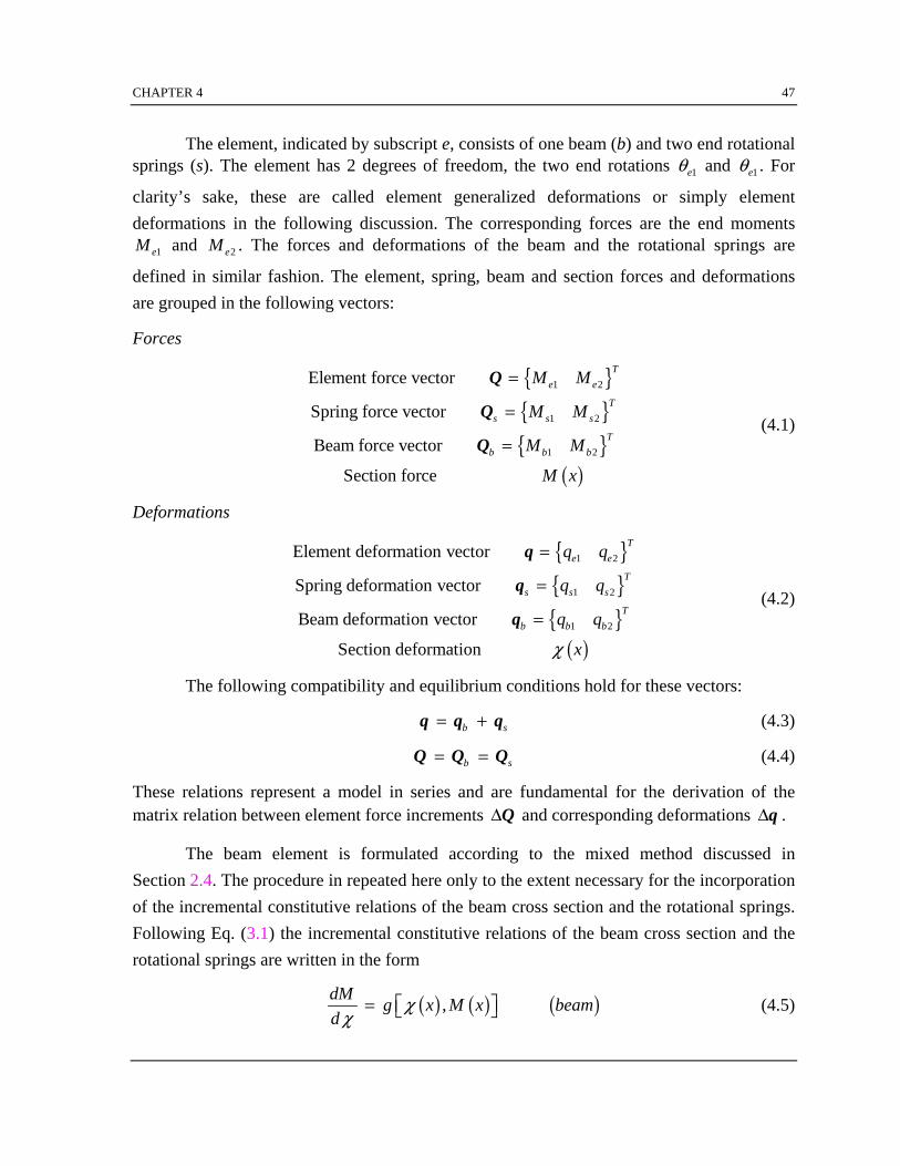
CHAPTER 4 47

The element, indicated by subscript e, consists of one beam (b) and two end rotationalsprings (s). The element has 2 degrees of freedom, the two end rotations 1eq and 1eq . For

clarity’s sake, these are called element generalized deformations or simply elementdeformations in the following discussion. The corresponding forces are the end moments

1eM and 2eM . The forces and deformations of the beam and the rotational springs are

defined in similar fashion. The element, spring, beam and section forces and deformationsare grouped in the following vectors:

Forces

{ }{ }{ }

( )

1 2

1 2

1 2

Element force vector

Spring force vector

Beam force vector

Section force

Te e

Ts s s

Tb b b

M M

M M

M M

M x

=

=

=

Q

Q

Q(4.1)

Deformations

{ }{ }{ }( )

1 2

1 2

1 2

Element deformation vector

Spring deformation vector

Beam deformation vector

Section deformation

Te e

Ts s s

Tb b b

q q

q q

q q

xc

=

=

=

q

q

q(4.2)

The following compatibility and equilibrium conditions hold for these vectors:

b s= +q q q (4.3)

b s= =Q Q Q (4.4)

These relations represent a model in series and are fundamental for the derivation of thematrix relation between element force increments DQ and corresponding deformations Dq .

The beam element is formulated according to the mixed method discussed inSection 2.4. The procedure in repeated here only to the extent necessary for the incorporationof the incremental constitutive relations of the beam cross section and the rotational springs.Following Eq. (3.1) the incremental constitutive relations of the beam cross section and therotational springs are written in the form

( ) ( ) ( ),dM g x M x beamd

cc

È ˘= Î ˚ (4.5)

48 CHAPTER 4

( ) ( ), 1, 2slsl sl sl

sl

dM g M l springsd

qq

= = (4.6)

For the beam cross section the constitutive law describes a differential moment-curvature relation, while for the end rotational springs it represents a differential moment-rotation relation. According to the numerical integration procedure in Chapter 3, Eqs. (4.5)and (4.6) become

( ) ( ) ( ) ( ) ( )1 1j j j jx f x M x r x beamc - -D = D + (4.7)

( )1 1 1, 2j j j jsl sl sl slf M r l springsq - -D = D + = (4.8)

where f is the section or spring flexibility and r denotes the residual curvature or rotation.The latter arises from the consistent linearization of the nonlinear constitutive laws in Eqs.(4.5) and (4.6), as discussed in detail in Chapter 3. Even though the formal representation ofthe force-deformation behavior of the beam cross section and the end rotational springs is thesame, different material parameters can be used in each case, as necessary. The materialparameters of the incremental constitutive relations were introduced in Chapter 3 and will bediscussed in more detail in Chapter 5.

The matrix relation between forces and corresponding deformations of the endrotational springs can be readily obtained from the constitutive relation of each spring andthe fact that the response of each spring is independent from the other. Consequently,

1 1j j j js s s s

- -D = D +q F Q s (4.9)

where

1 1

2 2

00s s

s ss s

f rf r

È ˘ Ï ¸= = Ì ˝Í ˙Î ˚ Ó ˛

F s (4.10)

The spring flexibility and the residual deformations are determined according to Eq. (3.29).

The matrix relation between end forces and corresponding deformations of the beamis derived in accordance with the mixed formulation of Chapter 2. The combination of theincremental constitutive law for the beam cross section in Eq. (4.7) with the mixed method ofSection 2.4 results in the following matrix relation

1 1j j j jb b b b

- -D = D +q F Q s (4.11)

where bF is the flexibility matrix of the beam and is obtained according to

CHAPTER 4 49

( ) ( ) ( )0

L

Tb x f x x dx= ÚF b b (4.12)

while bs are the residual deformations at the ends of the beam and are obtained according to

( ) ( )0

L

Tb x r x dx= Ús b (4.13)

At this point the matrix relation between end force increments and correspondingdeformations for the entire beam element can be established from the compatibility andequilibrium conditions in Eqs. (4.3) and (4.4), which are now written in incremental form

j j jb sD = D + Dq q q (4.14)

j j jb sD = D = DQ Q Q (4.15)

The combination of Eqs. (4.9), (4.11) and (4.14) yields the following relation1 1 1 1j j j j j j j

b b b s s s- - - -D = D + + D +q F Q s F Q s (4.16)

or,1 1j j j j- -D = D +q F Q s (4.17)

where F is the flexibility matrix of the entire beam element, as the sum of the flexibilities ofthe beam and the end springs

b s= +F F F (4.18)

and s are the residual deformations of the entire beam element, as the sum of thecorresponding residual deformations of the beam and the end springs

b s= +s s s (4.19)

Eq. (4.17) is the matrix relation between end force increments and correspondingdeformations for the entire beam element. The corresponding element state determination isvery similar to the procedure discussed in Chapter 2. At this point it is important to note thatthe end deformation increments are such that 1j=D πq 0 and 1j>D =q 0 , as was discussed in

Chapter 2. In the first element iteration the end deformation increments are obtained from thenodal displacement increments at the structural degrees of freedom. In the subsequentiterations the nodal displacements and corresponding deformations cannot change, so as notto violate compatibility. Since ( )1 1j j j- -D = ◊ -Q K s for j>1 according to the state

determination procedure in Chapter 2, it is easy to conclude from Eq. (4.17) that 1j>D =q 0 .

50 CHAPTER 4

The element formulation in this study is almost identical to the procedure used in theparallel study for a beam-column element by Taucer et al. (1991). The latter involves anexplicit section constitutive law that is derived from the nonlinear material behavior of thefibers into which the section is divided and the hypothesis that plane sections remain plane.The stiffness matrix and resisting forces of the section are derived by integration of thestiffness and resisting stress of the fibers. The difference between applied and resisting forcesat the section results in a force unbalance that yields a residual deformation when multipliedby the new section stiffness. By contrast, in the present study the section constitutive relationis only known in the incremental form of Eq. (4.7). While the overall element statedetermination procedure remains the same, the section state determination is clearly affectedby the different section behavior.

4.3 Numerical Integration

All integrals in the element formulation are evaluated numerically with the Gauss-Lobatto integration scheme that is based on the expression

1 1

1

21

( ) ( 1) ( ) (1)m

h h m

h

I g d w g w g w gx x x-

=-

= ◊ = ◊ - + ◊ + ◊ÂÚ (4.20)

where h denotes the monitored section and hw is the corresponding weight factor (Stroud

and Secrest 1966). The Gauss-Lobatto scheme with m integration points permits the exactintegration of polynomials of degree up to (2m-3). This procedure is superior to the classicalGauss integration method, when it is important to include in the integration the end points ofthe element. Since inelastic behavior in beam-column elements often concentrates at the endsof the member, the monitoring of the end sections of the element offers advantages from thestandpoint of accuracy and numerical stability.

4.4 Element State Determination

The state determination for the entire beam element follows the procedure describedin Chapter 2. During this phase of the algorithm the task at hand is the determination of theelement stiffness matrix and resisting forces for given end displacements. The numericalimplementation of the element state determination is summarized in the following step-by-

CHAPTER 4 51

step description. It is important to recall that the nonlinear solution algorithm for the entirestructure is subdivided into three nested loops:

Loop k denotes the sequence of load increments kEDP for the application of external loads

on the structure. At load step k the total applied load is kEP .

Loop i denotes the iteration scheme at the structural degrees of freedom, i.e. the structurestate determination. for the determination of the structural displacements kP thatcorrespond to the applied loads k

EP . In the present study the Newton-Raphson

algorithm is used for the purpose.

Loop j denotes the iteration scheme at the element level, i.e. the element statedetermination process. These iterations are necessary for the determination of theelement resisting forces that correspond to deformations iq at the i-th Newton-

Raphson iteration.

The relation and interaction among these three iteration processes is explained in more detailin Taucer et al. (1991) with a few illustrative diagrams. The following discussion is limitedto one Newton-Raphson step i and concentrates on the steps of iteration loop j.

In Newton-Raphson step i the displacement increments iDp at the structural degrees

of freedom are established first from the solution of the global equilibrium equations. Thenext task involves the determination of the stiffness matrix and resisting forces of thestructure that correspond to the new structural displacements ip . This entails the following

operations of state determination for each beam finite element:

(1) Determine the element deformation increments for Newton-Raphson step i.

Using the compatibility matrix eleL the element deformation increments iDq aredetermined from the nodal displacement increments iDp at Newton-Raphson step i

i ieleD = Dpq L

The compatibility matrix eleL performs, both, the elimination of rigid body modes

and the rotation to the local reference system.

(2) Update the element deformations.

1i i i-= + Dq q q

52 CHAPTER 4

(3) Start the element state determination.

Set the index of the first iteration: j=1.

(4) Determine the element force increments.

The element force increments jDQ are determined with the element stiffness matrix1j-K at the end of the previous iteration in loop j. There are two cases:

a) for j=1

1 0j j i= =D = DQ K q

b) for j>1

( )1 1j j j- -D = -Q K s

where 1j-s are the residual element deformations at the end of the previous iteration,as determined in step (13) below.

(5) Update the element forces.

1j j j-= + DQ Q Q

When j=1, 0 1i-=Q Q where i-1 indicates the previous Newton-Raphson iteration.

From equilibrium the forces in the beam and end springs are equal to the elementforces, so that:

j j j j j js b s bD = D = D = =Q Q Q Q Q Q

(6) Determine the force increments at the control sections of the beam.

The section force increments ( )jhM xD are determined from the force interpolation

functions b(x) and the element force increments jDQ . The section force ( )jhM x is

then updated. These operations are repeated for all control sections or integrationpoints m in the beam.

( ) ( ) 1,j jh hM x x h mD = D =b Q

1( ) ( ) ( ) 1,j j jh h hM x M x M x h m-= + D =

CHAPTER 4 53

(7) Determine the deformation increments at beam control sections and end springs.

The deformation increments ( )jhxcD and j

sDq are determined by adding the residualdeformations from the previous iteration, 1( )j

hr x- and 1js-s , to the deformation

increments due to force increments ( )jhxMD and j

sDQ , respectively.

1 1( ) ( ) ( ) ( ) 1,j j j jh h h hx f x M x r x h mc - -D = D + =

1 1j j j js s s s

- -D = D +q F Q s

The corresponding vectors are then updated

1( ) ( ) ( ) 1,j j jh h hx x x h mc c c-= + D =

1j j js s s

-= + Dq q q

(8) Determine the error function and its derivatives.

Compute the error function and its derivatives at the beam control sections, ( )jhxy ,

( )jhx∂y

∂c and

( )jhx

M∂y∂

for h=1..m and at the end springs, jsly ,

j

sl

∂y∂q

and j

slM∂y∂

for

l=1..2.

(9) Determine the flexibility at the beam control sections and the end springs.

Determine the section flexibility

( )( )

( ) 1,

jh

jh j

h

xMf x h m

x

∂y∂

∂y∂c

= - =

and the diagonal spring flexibility matrix jsF with the following terms

1,2

j

j slsl j

sl

Mf l

∂y∂∂y∂q

= - =

(10) Determine the residual deformations at the beam control sections and end springs.

Determine the residual section deformations

54 CHAPTER 4

( ) ( )( ) 1,

jhj

h jh

xr x h m

xy∂y

∂c

= - =

and the residual spring deformation vector jss with the following terms

1,2j

j slsl j

sl

r ly∂y∂q

= - =

(11) Determine the flexibility matrix of the beam and the entire element .

The flexibility matrix of the beam is obtained by numerical integration of sectionflexibilities

1

( ) ( ) ( )m

j T jb h h h h

h

w x f x x=

È ˘= Î ˚ÂF b b

The flexibility matrix of the entire element is then established as the sum of the beamand end spring flexibility matrices

j j jb s= +F F F

(12) Determine the element stiffness matrix.

Invert the element flexibility to obtain the element stiffness matrix

1j j -È ˘= Î ˚K F

(13) Check for element convergence.

a) If the error function is sufficiently small at all control sections of the beam and atthe end springs, the element state determination process has converged.

b) If the error function exceeds the specified tolerance at one or more controlsections, the residual deformations of the beam and the entire element, j

bs andjs , respectively are determined.

1

( ) ( )m

j T jb h h h

h

w x r x=

È ˘= Î ˚Âs b

CHAPTER 4 55

j j jb s= +s s s

Steps (4) through (13) are repeated until the error function is sufficiently small at allcontrol sections of the beam and at the end springs.

1hM

1 1h hM b Q∆ = ∆

0hχ 2

hχhχ

0curve ψ=

0 1h hf M∆

1hχ

1hr

1 2h hf M∆

0hf

11hf

2 2h hM b Q∆ = ∆2

hM

1hM

0hM 0

1 2

FIGURE 4.3 STATE DETERMINATION AT MONITORED SECTION h

Q

1Q

0Q

1 0 iQ K q∆ = ∆

q1iq − iq

iq∆

0K 1K

( )2 1 1Q K s∆ = −2Q

1s

0

1

2

FIGURE 4.4 STATE DETERMINATION OF BEAM ELEMENT

56 CHAPTER 4

The first two iterations of the element state determination are schematically shown inFigs. 4.3 and 4.4. Fig. 4.3 refers to monitored section h and Fig. 4.4 to the beam element. Inboth figures 0 denotes the initial point of the element state determination. For the firstelement iteration j=1, the section force increment 1 1

h hMD = Db Q is determined from theelement force increment 1 0 iD = DQ K q and the force field is updated to 1 0 1

h h hM M M= +D .The initial flexibility 0

hf yields the corresponding curvature increment 1 0 1h h hf McD = D

according to the consistent linearization of the constitutive relation. Given the initial point( 0 0,h hMc ) and the two increments 1

hcD and 1hMD the error function 1

hy and its partialderivatives 1 1

h M∂y ∂ and 1 1h∂y ∂c can be established yielding the section flexibility 1

hfand residual curvature 1

hr . In order to maintain compatibility at the element nodes the

correction of the residual section curvatures is deferred to the next iteration in loop j. Thesection flexibility and the residual curvatures are integrated to obtain the beam flexibility 1

bFand the residual deformations 1

bs . The same procedure is followed for the end springsyielding the spring flexibility 1

sF and the residual deformations 1ss . In the next step the

element flexibility 1F and the residual deformations 1s are determined, thus completing thefirst iteration j=1. Point 1 corresponds to the final point of the first iteration in Figs. 4.3 and4.4. The residual element deformations at the end of the previous iteration yield the elementforce increment for the iteration j=2 according to ( )2 1 1D = -Q K s . The corresponding section

force increment 2 2h hMD = Db Q is determined and the entire force field is updated to

2 1 2h h hM M M= +D . The section curvature increment is then determined with

2 1 2 1h h h hf M rcD = D + and the corresponding vector is updated. The new error function 2

hy andits partial derivatives 2 2

h M∂y ∂ and 2 2h∂y ∂c are established yielding the new section

flexibility 2hf and residual curvature 2

hr . The section flexibility and the residual curvaturesare integrated to obtain the beam flexibility 2

bF and the residual deformations 2bs . The spring

flexibility and residual deformations are also computed. Finally, the element flexibility 2Fand the residual deformations 2s are established, thus completing the second iteration j=2.Point 2 corresponds to the final point of the second iteration in Figs. 4.3 and 4.4. Theiterations continue until the error function becomes sufficiently small at all control sectionsof the beam and at the end springs.

It is important to point out that the deformations q of the entire element do not

change during the iterations of the element state determination process. By contrast, thedeformations of the beam and springs, bq and sq , respectively, change during these

CHAPTER 4 57

iterations. For the new element deformations 1i i i-= + Dq q q the deformations of the beam

and springs are adjusted until the corresponding constitutive relations are satisfied within thespecified tolerance. During the iteration process compatibility is always maintained, since thesum of sq and bq is equal to iq , even though the individual contributions vary. This is an

important characteristic of the model showing the application of the flexibility-based methodand the proposed state determination process to a finite element that is formed by a beam andtwo end springs connected in series. Given the imposed nodal deformations iq , the forces

and deformations of the beam and end springs are adjusted until the element forces Q and thecomponent deformations bq and sq satisfy the corresponding constitutive relations whilemaintaining compatibility between the components, as expressed by b s= +q q q , andequilibrium, as expressed by b s= =Q Q Q and ( )( )M x x= b Q . In this particular model

implementation, the compatibility between the components need only be maintained at theend nodes, while the equilibrium is satisfied in a strict sense along the beam, as ensured bythe internal force distribution ( )( )M x x= b Q .

59

CHAPTER 5

MODEL PARAMETERS AND DEGRADATION SCHEME

5.1 General

This chapter discusses the selection of parameters for the incremental constitutiverelation of Chapter 3. This constitutive relation was used in Chapter 4 to describe themoment-curvature relation of the beam control sections and the moment-rotation relation ofthe end springs. Since both constitutive relations are not necessarily symmetric, two sets ofparameters are needed: one controls the behavior of the model in the positive load-deformation regime and the other in the negative. With the change in value of the controlparameters during the loading history, the model can trace hysteretic loops of various shapeswith different initial, unloading and post-yield stiffness.

The first part of the chapter discusses the basic constitutive law developed in Chapter3. In the second part the basic model is extended to include the effect of “pinching”. Thiseffect of the hysteretic behavior is characteristic of materials that exhibit soft response underreloading for deformations that do not exceed the maximum previously imposed. Because ofshear cracking and bond slip during cyclic loading, reinforced concrete is a material thatexhibits such behavior. In the proposed model pinching is included by defining a lowerintermediate level of yielding and a corresponding post-yield (pinching) stiffness. The lastpart of the chapter introduces the scheme of degradation of model parameters. As loadingprogresses, steel and concrete structural members often exhibit gradual degradation ofstrength and stiffness and a consequent loss of dissipative capacity. Damage is anevolutionary process that can be naturally included in an incremental constitutive relation. Adamage coefficient is defined for each model parameter as the weighted sum of total plasticwork and maximum deformation. Damage is assumed to be symmetric, so that the samedamage coefficients affect the model parameters in the positive and negative load-deformation regime. The chapter concludes with a summary of the model and degradationparameters.

60 CHAPTER 5

5.2 Parameters for Incremental Constitutive Law

Chapter 3 presented the development of an incremental constitutive law from asimple standard solid model. This constitutive relation was used in Chapter 4 to describe themoment-curvature relation of the beam control sections and the moment-rotation relation ofthe end springs. The parameters defining the incremental law are described in this section,limiting attention to the moment-curvature relation and keeping in mind that the moment-rotation relation of the end rotational springs has exactly the same form.

The moment-curvature relation in Eq. (3.17) can be written as follows after recallingthat 0 0 0M EI c= ◊

( ) ( ) ( ){ }0 1 1 ndM EI sgn d sgn x xd

a c b gc

È ˘= - - +Î ˚ (5.1)

where

0 1 2EI EI EI= + (5.2)

2

0

EIEI

a = (5.3)

( ) ( )0 01 1Mx

Mc a

a c a= -

- -(5.4)

For the moment-rotation relation that characterizes the behavior of the end rotationalsprings, Eq. (5.1) can be written in the same way, by replacing 0EI with 0k , c with q and

using the definition of a in Eq. (5.3). In order to allow for non-symmetric load-deformationbehavior two sets of parameters are needed for Eq. (5.1): one controls the behavior of themodel in the positive load-deformation regime and the other in the negative. Only theunloading parameters g and b have a single value. In the following description only the

behavior of the model in the positive load-deformation regime will be discussed, theextension to the negative regime being straightforward. At the end of the chapter Table 1summarizes the parameters that control the constitutive law of the beam cross sections andthe end rotational springs.

The parameters in Eq. (5.1) are illustrated in Fig. 5.1. E is the initial elastic modulusof the material and I the moment of inertia of the cross section. 0EI is the initial tangentstiffness of the moment-curvature relation and 2EI is the post-yield stiffness. 0M is the yield

moment which for the model represents the bending moment at the intersection of the initial

CHAPTER 5 61

tangent stiffness and the linear asymptote of the moment-curvature relation for very largecurvature values. Parameter a represents the strain hardening ratio between the post-yieldstiffness and the initial elastic stiffness of the model.

1.2

0

-1.2-6 0 6

2 0EI EIα=

2EI

0EI

( )0 0,M χM

χ

FIGURE 5.1 PARAMETERS DEFINING THE BEHAVIOR OF THE BASIC CONSTITUTIVE LAW

0

1

0.5

1.02.0

5.0100

10.0

2 4

M

χ

n = 0.5

FIGURE 5.2 INFLUENCE OF n ON TRANSITION FROM ELASTIC TO PLASTIC BRANCH

62 CHAPTER 5

Exponent n in Eq. (5.1) governs the transition from the elastic to the elasto-plasticbranch. Its influence on the moment-curvature response is depicted in Fig. 5.2: small valuesof n lead to a smooth transition, but as n increases the transition becomes sharper tending to aperfectly bilinear behavior in the limit.

In Eq. (5.1) g and b are two parameters that govern the initial phase of the

unloading paths. Since their sum equals 1 according to the discussion in Section 3.2, onlyone parameter can be selected independently. In the following discussion g in the variableparameter. The value 0.5g = is the default selection that gives rise to linear elasticunloading with the same slope 0EI as the initial loading. If g is assigned a value smallerthan 0.5, the slope becomes steeper. It is important to recall that g may take any positive or

negative value smaller or equal to 0.5 according to Section 3.2. Fig. 5.3 shows threehysteretic loops corresponding to 0.5g = , 3g = - and 200g = - . The effect of g on the

hysteretic behavior may be rather sensitive to the size of unloading deformation increments.With larger increments the unloading path tends to perfectly elastic behavior, thusdiminishing the effect of g .

-0.006 0 0.006

0

800

1600

-800

-16000.003-0.003

γ = 0.5-3

-200

M

χ

FIGURE 5.3 INFLUENCE OF UNLOADING PARAMETER g ON M c- CURVE

5.3 Pinching

The hysteretic behavior of some materials is characterized by soft response under

CHAPTER 5 63

reloading for deformations that do not exceed the maximum previously imposed. Because ofshear cracking and bond slip during cyclic loading, reinforced concrete is a material thatexhibits such “pinching” behavior. The model of Chapter 3 can be modified to include theeffect of “pinching” by introducing a new set of parameters. The idea is to define anintermediate fictitious yield level at the moment value that corresponds to the onset of“pinching” and an intermediate set of parameters similar to those described in Section 5.2.These intermediate values control the hysteretic behavior of the model until a specifieddeformation value is reached.

Formally, this is accomplished by rewriting Eq. (5.1) in the more general form

( ) ( ) ( ){ }0 1 1 ndM EI sgn d sgn x xd

a c b gc

È ˘= - - +Î ˚ (5.5)

where

( ) ( )0 01 1Mx

Mca

a c a= -

- -(5.6)

00

0

MEI

c = (5.7)

2

0

EIEI

a = (5.8)

( )2 2 2 2P PEI EI EI EI c= + - (5.9)

( )0 0 0 0P PM M M M c= + - (5.10)

( )P Pn n n n c= + - (5.11)

Superscript P stands for “pinching”. Fig. 5.4 illustrates these new parameters. 0PM is the

moment value at the intersection of the “pinching” branch with the bending moment axis,and 2

PEI is the stiffness of the “pinching” branch. Similar to n in Eq. (5.1), Pn is the

exponent governing the transition from the elastic reloading branch to the “pinching” branch.0EI , 2EI , 0M , n and g are the same parameters defined in Section 5.2. Eqs. (5.9)-(5.11)

depend on a parameter c, that relates the basic model parameters with the parameters for the“pinching” branch and defines the curvature value at the onset of “pinching”. It is defined bythe following expression:

64 CHAPTER 5

-0.25 -0.15 -0.05 0.05 0.15 0.25

1.8

1.2

0.6

0

-0.6

-1.2

0M

0PM

Pn

1c

2PEI

M

χ

FIGURE 5.4 PINCHING PARAMETERS AND THEIR EFFECT ON CONSTITUTIVE LAW

12

2

for1 for

normax

max

ce ccc

c c cc c

Ï <Ô= Ì>ÔÓ

(5.12)

-2 0 2

30

0

-30

1c = 0.3

0.1

3.0

M

χ

FIGURE 5.5 INFLUENCE OF PARAMETER 1c ON TRANSITION FROM

PINCHING BRANCH TO PREVIOUS RELOADING BRANCH

CHAPTER 5 65

where 1c is an arbitrary coefficient whose effect on the shape of the “pinching” branch andthe transition to the original reloading branch is shown is Fig. 5.5. 2 maxc c is a limitdeformation value that is specified below, and norc is a normalized deformation given by the

expression

( ) 2

0

maxnor

sgn d cc c cc

c◊ - ◊

= (5.13)

In Eqs. (5.12) and (5.13), 2c is a positive coefficient and maxc is the maximum deformationvalue in all previous loading cycles. Under negative deformation increments maxccorresponds to the maximum negative deformation value in all previous loading cycles maxc - ,

and under positive deformation increments it corresponds to the maximum positivedeformation value maxc + . The effect of different values of 2c on the transition from the“pinching” branch to the original reloading branch is shown in Fig. 5.6. If 2 0c = , the

transition from the “pinching” branch to the original reloading branch initiates at zerocurvature. At the other extreme, if 2 1c = the transition from the “pinching” branch to the

original reloading branch is delayed until the maximum deformation value experienced inprevious cycles. Even though it seems reasonable to assume that [ ]2 0,1c Π, the model canalso be assigned values of 2c larger than 1, as shown in an application of the model in

Chapter 6.

1.2

0

-1.2-6

0.51.0

0.00.51.0

0 6

0.0

maxχ−

2c =

maxχ+

M

χ

FIGURE 5.6 INFLUENCE OF PARAMETER 2c ON TRANSITION FROM PINCHING BRANCH

66 CHAPTER 5

-20 00

0.50.25

0.1

1.05.0

norχ

c

0.051c =

1( ) 2

0

sgn maxnor

d cχ χ χχχ−

=

1 norcc e χ=

FIGURE 5.7 INFLUENCE OF 1c ON c AS THE NORMALIZED CURVATURE norc INCREASES

The behavior of parameter 1 norcc e c= is analyzed in Fig. (5.7). For a small value ofcurvature c , norc assumes a very small negative value and c tends to zero, so that theparameters for the “pinching” branch dominate the response in Eq. (5.5). As the curvature cincreases and approaches the value 2 maxc c , norc tends to zero and c tends to 1, so that the

parameters of the initial reloading branch dominate the response in Eq. (5.5). The rate atwhich c increases form 0 to 1 depends on 1c . At the limit, as 1c Æ• , c becomes a deltafunction ( )2 maxc cd c c= - , where ( )xd is the Dirac delta function, equal to 1 for x=0 and

otherwise equal to zero.

5.4 Degradation Scheme

Experimental results of the hysteretic behavior of steel and reinforced concretemembers show that repeated deformation cycles can cause deterioration of strength andstiffness of the member. Damage is an evolutionary process that can be naturally included inan incremental constitutive relation. A damage coefficient is defined for each modelparameter as the weighted sum of total plastic work and maximum deformation. Damage isassumed to be symmetric, so that the same damage coefficients affect the model parametersin the positive and negative load-deformation regime. Typically, damage indices assumevalues in the interval between 0 and 1 and decrease monotonically with increasing damage

CHAPTER 5 67

from the value of 1, which characterizes no damage, to the value of 0, which representscomplete damage.

It it rather straightforward to introduce progressive damage in the constitutive relationthat is defined by Eqs. (5.1) and (5.5). If W stands for the generic model parameter, nW and

1n+W denote the parameter values at the end of the global load steps n and n+1, respectively,

according to the notation of Chapter 3. The degradation scheme follows the equation

( )1 1 1 21n n nW d dW+ +W = W - D (5.14)

where 1dW and 2d are two parameters that will be defined subsequently, and 1nW +D is theplastic work during the global step n+1. 1nW +D is determined from the expression

( )1 11 2

pn n n

n

M MW

c+ ++

+ DD = (5.15)

where 1p

nc +D is the plastic deformation increment, which according to Eq. (3.9) is

( )( )

2

0 1

n

p M EIw

Mc

c ca

-D = D

-(5.16)

The degradation scheme defined by Eq. (5.14) is applied to the following modelparameters: 0EI , 2EI , 0M , 0

pM , a , n , pn , 1c , 2c . Note that Eq. (5.14) is not dimensionallycorrect, because every term is dimensionless except for the plastic work increment 1nW +D .

This increment could be normalized by dividing the right hand side of Eq. (5.15) by ameasure of the work stored at yielding of the material, as defined by the product 0 0M c .

Since this correction is not necessary for low-cycle fatigue, which is the main focus of thisstudy, it is not included in the present implementation of the element whose degradationscheme follows Eqs. (5.14) and (5.15) and should be used with care in cases of high-cyclefatigue.

The two coefficients 1dW and 2d in Eq. (5.14) control the weighting between plastic

work and maximum deformation amplitude in the definition of damage. The first coefficient1dW varies in the range of [0,1]: if 1 0dW = , damage is only a function of maximum

deformation amplitude and does not depend on plastic work; if 1 1dW = , the reverse is true.

Superscript W stands for the generic model parameter to indicate that one damagecoefficient is defined for each model parameter, without distinction between the parametersthat control the behavior of the model in the positive and in the negative load-deformationregime. For example, 0

1EId governs the degradation of, both, positive and negative initial

68 CHAPTER 5

stiffness, 0EI + and 0EI - , respectively. All damage coefficients 1dW that need to be specified

for the definition of the hysteretic behavior of the constitutive relation are summarized inTable 1 at the end of this chapter.

The second coefficient 2d is unique for all model parameters and is defined by

12

21

1

1ampbb

d

ecÊ ˆ

◊ -Á ˜Ë ¯

=

+

(5.17)

ampc is a deformation amplitude that controlls the degradation process and is, in turn,

defined by

( )max 3 max maxamp bc c c c+ + -= - - (5.18)

02 4

1

0.5

123510

1 3 5

2d

0.51b =

2amp bχ

12

21

1

1ampbb

d

eχ⎛ ⎞⎟⎜ ⎟−⎜ ⎟⎜ ⎟⎜⎝ ⎠

=

+

0

FIGURE 5.8 INFLUENCE OF PARAMETER 2b ON 2d FOR DIFFERENT VALUES OF 1b

3b is a coefficient that controlls the relative influence of the maximum and minimum

deformation amplitudes on the degradation. Its value ranges from 0 to 1: the value of 0ensures that degradation only depends on the maximum (positive) deformation amplitude,while the value of 1 limits the effect only to the minimum (negative) deformation amplitude.The value of 0.5 assigns equal weight to the extreme deformation values maxc + and maxc - .Fig. 5.8 shows the effect of parameters 1b and 2b on the degradation parameter 2d . If 1b issmall, the degradation effect increases smoothly as the curvature amplitude increases. As 1b

CHAPTER 5 69

becomes larger, 2d tends to a unit step function equal to 0 for 2amp bc < and equal to 1 for

2amp bc > .

0 0.004 0.0080

1500

1000

500

0.05

0.1

0.2

0.4

0.025

1

2

3

bbb

===

100

0.001

0

02Md = 0M

χ

FIGURE 5.9 EFFECT OF DEGRADATION OF YIELD MOMENT 0MON YIELD AND POST-YIELD BEHAVIOR

The following figures illustrate the effect of the degradation degree of key modelparameters on the hysteretic behavior of the model. Fig. 5.9 shows the monotonic behavior ofthe model for increasing values of 0

1Md and, thus, for increasing degradation of the yield

moment 0M . As the imposed deformation increases, the yielding level decreases and the

model exhibits a gradual loss of strength. This simulates well the characteristic strainsoftening behavior of certain materials, such as plain or reinforced concrete.

Fig. 5.10 shows the effect of degradation of yield moment and initial stiffness on thehysteretic behavior of the model under fixed deformation cycles of equal positive andnegative amplitude. Fig. 5.10a isolates the effect of degradation of the yield moment only,Fig. 5.10b isolates the effect of degradation of the elastic stiffness, and Fig. 5.10c shows thecombined effect of degradation of both parameters. The hysteretic behavior in Fig. 5.10 isobtained with a very low value for parameters 0

1Md and 0

1EId , since, otherwise, the large

value of plastic work during cyclic loading can quickly reduce the yield moment and theinitial stiffness to zero and, thus, yield unrealistic results. For the cases of Fig. 5.10 whichinvolve the degradation of yield moment, not only is the “pinching” level pM equal to theyield moment 0M , but the same degradation function is used for both, i.e. 0

1 1

pM Md d= . If this

is not the case, the hysteretic behavior changes to that in Fig. 5.11.

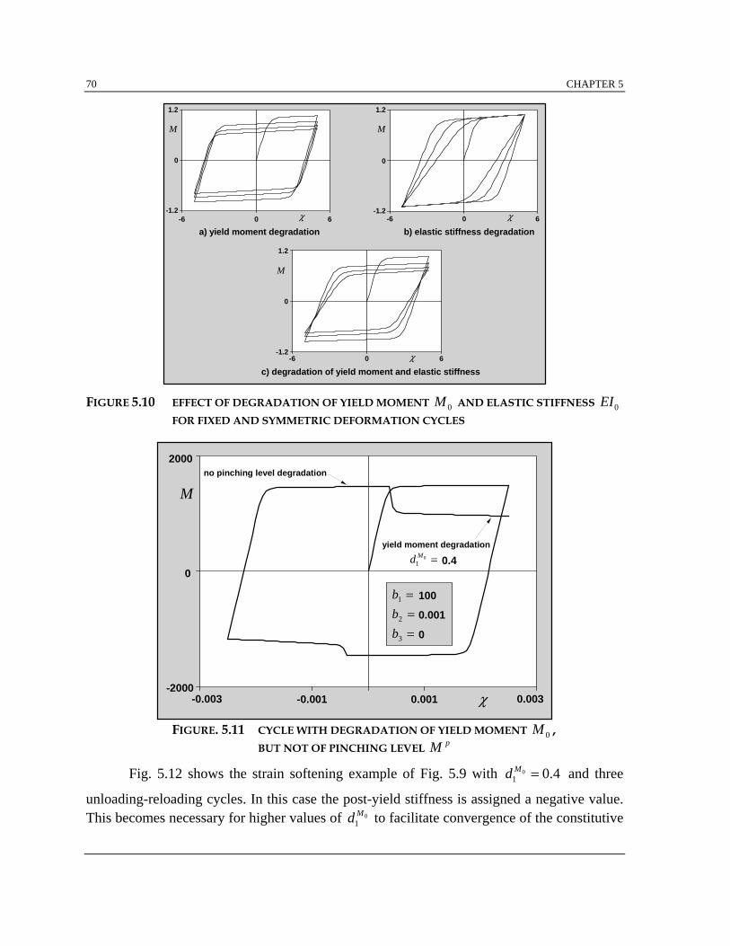
70 CHAPTER 5

1.2

0

-1.2-6 0 6

-6 0 6

1.2

0

-1.2

1.2

0

-1.2-6 0 6

b) elastic stiffness degradation

c) degradation of yield moment and elastic stiffness

a) yield moment degradation

M

c c

M

M

c

FIGURE 5.10 EFFECT OF DEGRADATION OF YIELD MOMENT 0M AND ELASTIC STIFFNESS 0EIFOR FIXED AND SYMMETRIC DEFORMATION CYCLES

-0.003 -0.001 0.001 0.003

2000

-2000

no pinching level degradation

yield moment degradation

00.4

bbb

1

2

3

===

100

0.001

0

M

c

d M1

0 =

FIGURE. 5.11 CYCLE WITH DEGRADATION OF YIELD MOMENT 0M ,BUT NOT OF PINCHING LEVEL pM

Fig. 5.12 shows the strain softening example of Fig. 5.9 with 01 0.4Md = and three

unloading-reloading cycles. In this case the post-yield stiffness is assigned a negative value.This becomes necessary for higher values of 0

1Md to facilitate convergence of the constitutive

CHAPTER 5 71

model. Degradation of the elastic stiffness is also specified ( 01 0.2EId = ). Three unloading

cycles to zero moment with reloading back to the envelope curve are specified. It isinteresting to observe that the model shows a physical inconsistency in the failure of theunloading-reloading cycles to close. A detailed discussion of this phenomenon is presentedin Appendix B in connection with the comparison of the proposed model with the Bouc-Wenmodel. It is possible to avoid this inconsistency by specifying a high initial value (seeFig. 5.2) and disallowing any degradation of exponent n, which controls the sharpness of thetransition from the linear elastic to the post-yield range of response.

0

2000

0 0.007

2000

0 0.007

0

b) with degradation of n

a) without degradation of the transition parameter n

bbb

1

2

3

===

1000.0010

d

d

d

M

EI

EI

1

1

1

0

0

2

=

=

=

d

d

d

M

EI

EI

1

1

1

0

0

2

=

=

=

0.40.20.4

M

c

M

c

dn1 = 0

d n1 = 0.2

FIGURE 5.12 POST-YIELD CYCLES WITH AND WITHOUT DEGRADATION OF n :DEGRADATION IS ALSO SPECIFIED FOR 0M , 0EI , AND 2EI

Finally, Fig. 5.13 shows that appropriate parameter selection enables the model toapproximate the characteristic monotonic post-yield axial behavior of a steel coupon thatexhibits a higher and lower yield stress and a plastic plateau followed by strain hardening.

72 CHAPTER 5

0 0.004 0.008

2

1

0

bbb

1

2

3

===

100

0.0010

d

d

M

EI

1

1

0

2

=

=

0.4

0.1

M

c

FIGURE 5.13 SIMULATION OF POST-YIELD BEHAVIOR OF

A STEEL COUPON UNDER MONOTONIC AXIAL LOADING

The few examples in this chapter demonstrate the inherent flexibility of the proposedconstitutive model and the wide range of monotonic and hysteretic behaviors that it cansimulate. Some correlation studies with experimental results are presented in the followingchapter.

The demonstrated flexibility of the proposed model and the interaction betweenseveral parameters make the parameter selection by trial and error a difficult and lengthyprocess. It is possible to find several parameter combinations that match reasonably well theobserved hysteretic behavior of a specimen. It is also possible to arrive at parametercombinations that lead to hysteretic behavior that is physically meaningless or eveninconsistent with the basic rheological model that forms the foundation of the proposedconstitutive relation. The latter problem arises, because of the purely empirical way ofintroducing the “pinching” effect in the basic model. So, while the introduction of the“pinching” effect in this chapter widens the range of hysteretic behaviors that the model cansimulate, it also gives rise occasionally to physically inconsistent response. For these reasonsobjective and systematic methods of parameter selection are superior to the trial and errorapproach. Such an objective method is based on system-identification: given an initial set ofparameters and a target moment-curvature relation, some user prescribed parameters aresuccessively updated until the error between the target curve and the model response is

CHAPTER 5 73

reduced to a prescribed minimum value. More details are provided in the work of Ciampi andNicoletti (1986).

PARAMETER SYMBOL DAMAGECOEFFICIENT

cross section area A

integration scheme q

beam unloading scheme bg

spring unloading scheme sg

tangent modulus E+ E- 01EId

moment of inertia I + I -

yield moment yM +yM -

1yMd

pinching moment M + M -1Md

post-yield stiffness 2EI +2EI - 2

1EId

post-pinching stiffness pEI+ pEI

-

1

pEId

transition at yielding n+ n-1nd

transition at pinching pn+ pn

-

1

pnd

transition at unloading 1c+1c- 1

1cd

parameter extension of pinching 2c+2c- 2

1cd

general degradation parameter 1 1b

general degradation parameter 2 2b

general degradation parameter 3 3b

TABLE 5.1 SUMMARY OF PARAMETERS FOR INCREMENTAL CONSTITUTIVE

RELATION AND OF CORRESPONDING DAMAGE INDICES

75

CHAPTER 6

APPLICATIONS

6.1 General

This chapter presents a few examples of the use of the proposed beam element in thesimulation of the hysteretic behavior of structural members. The beam element is presentlyimplemented in the general purpose finite element program ANSR. Details on the programcan be found in Mondkar and Powell (1975a) and (1975b).

The example of a softening cantilever beam monotonically displaced beyond its pointof maximum resistance is presented first. This is a test case for beam elements, because it iswell known that stiffness based elements, which start from the compatibility rather than theequilibrium conditions along the element, encounter serious numerical difficulties in tracingthe load-displacement behavior of softening members. The proposed beam element showsexcellent agreement with the experimental results and convergence is attained in fewiterations in every load step. Two more applications of the model are presented that comparethe analytical results with experimental evidence from two reinforced concrete cantileverbeams with non-symmetric longitudinal reinforcement. The first beam was cycled betweenfixed displacement values: in the experiment the beam failed in the second cycle when thebottom steel fractured. The second beam was cycled between symmetric displacements ofincreasing amplitude until failure took place. The finite element analysis of the two beamsshows good agreement with the experimental results. The chapter concludes with adiscussion about the selection of model parameters and damage coefficients and how theserelate to the physical behavior of a reinforced concrete member.

6.2 A Softening Cantilever Beam

Several recent studies have dealt with the simulation of the softening behavior ofreinforced concrete frame elements. Zeris and Mahin (1988) present a comprehensive reviewof these studies. The problem can be summed up as follows: when a cantilever element issubjected to an increasing displacement at the free end, the curvatures and bending moments

76 CHAPTER 6

increase along the beam until the maximum resistance is reached at the built-in end. For thesubsequent increase of tip displacement, the curvature amplitude increases in theneighborhood of the built-in end and decreases elsewhere in the beam, while the bendingmoment decreases along the beam, but remains linear in order to satisfy equilibrium. Thus,while the beam section at the built-in end softens, the remainder of the beam unloads, as thesections follow the decrease of bending moment in accordance with the reduction of themoment at the built-in end. The classical displacement method has difficulty tracing thisbehavior. In fact, following the common assumption of cubic displacement interpolationfunctions, that result in a linear curvature distribution, the element attempts to unload afterthe maximum resistance is reached at the built-in end. This unloading occurs in agreementwith the imposed element compatibility condition and the resulting linear curvaturedistribution, whereas, in reality, it is the linear bending moment diagram that needs to berespected.

The response of a cantilever beam with the proposed finite element is shown inFig. 6.1. The free end is supported on a very stiff spring to simulate an analysis underdisplacement control. The simple structure was studied with different mesh discretizations,but the response is mesh independent, as long as one rotational spring or one very short beamelement is inserted at the built-in end to ensure that the length of the inelastic region (plastichinge) remains constant. All beam sections have the same properties: the softening behavioris simulated by the degradation of the yield moment and by a negative post-yield stiffness.These two parameters need to be adjusted to obtain the desired degree of softening.

Fig. 6.1a shows the force-tip displacement relation. The softening behavior isgoverned by the moment-curvature history at the built-in section in Fig. 6.1b. After themaximum resisting moment is reached, the curvature at the built-in section continuesincreasing, whereas the resisting moment decreases. Accordingly, the tip displacementincreases, while the shear force decreases. The behavior of a typical intermediate section isdifferent in Fig. 6.1c. Since all sections respect the same constitutive relation and the bendingmoment diagram is linear, the sections along the beam are subjected to moment values lessthan the yield moment, when the built-in end reaches its maximum resistance. Once thebending moment decreases at the built-in section, all intermediate sections unload elasticallyto respect the imposed linear bending moment diagram. Fig. 6.1 shows that the proposedbeam element can easily represent this physical behavior. Furthermore, convergence is veryrapid, independent of mesh refinement and load step size. In fact, the load step size in theexample of Fig. 6.1 was conditioned by the desire to obtain a smooth diagram.

CHAPTER 6 77

This example makes clear why an approach based on force rather then displacementinterpolation functions is better suited to describe softening. This derives from the fact thatthe bending moment diagram is always linear in a beam without element loads,independently of its material behavior. On the other hand the curvature diagram is linear for

0

24

20

16

12

8

4

0

CURVATURE (rad/in)

a) BEAM LOAD-TIP DISPLACEMENT RESPONSE

SHEA

R F

OR

CE

(kip

s)

0

24

20

16

12

8

4

00.4 0.8 1.2 1.6 2 2.4

section A

section B

IMPOSED TIP DISPLACEMENT

p (in)

0.008 0.016 0.024 0 0.0001 0.0002 0.0003 0.0004

24

20

16

12

8

4

0

b) SHEAR FORCE-CURVATURESection A

c) SHEAR FORCE-CURVATURESection B

CURVATURE (rad/in)

P, p

SHEA

R F

OR

CE

(kip

s)

SHEA

R F

OR

CE

(kip

s)

FIGURE 6.1 MONOTONIC LOADING OF A SOFTENING CANTILEVER BEAM:BEHAVIOR AT THE BUILT-IN END AND AT AN INTERMEDIATE SECTION

78 CHAPTER 6

a prismatic beam with uniform linear elastic material, but becomes highly nonlinear in theinelastic region of the section constitutive relation. In the classical displacement formulationof a two node beam finite element, the curvature diagram is assumed linear and the bendingmoment diagram, though initially linear, becomes nonlinear as the section constitutive entersthe inelastic regime. This is in violation of the physical behavior. Even the proposed specialmethods, such as mesh refinement of the inelastic region of the member, do not free this typeof elements from serious numerical problems.

6.3 Correlation Study with Two Cantilever Specimens

In this section the experimental responses of two cantilever beams under cyclicloading are compared with the results obtained from the finite element analysis of the samebeams. The material properties, the geometry of the specimen and a discussion of theexperimental results are available in the study by Ma et al. (1976). Both beams are half-scalemodels of a typical beam in the critical region of a 20 story ductile moment-resistingconcrete frame. The beams have a rectangular cross section with non- symmetric longitudinalreinforcement: the top reinforcement consists of 4 #6 reinforcing bars and the bottomreinforcement consists of 3 #5 bars. Following the notation in Ma's work, the beams arereferred to as specimens R-3 and R-4. Details on specimen geometry and reinforcementlayout are given in Figs. 2.4 and 2.7 of Ma's work. The selection of these two specimens was

1

2 3

48.5"7"1" 7"

P, δ

4

FIGURE 6.2 FINITE ELEMENT MESH FOR CANTILEVER SPECIMENS R-3 AND R-4

CHAPTER 6 79

conditioned by the fact that their behavior was dominated by flexure and the effect of shearwas rather small, because of the span to depth ratio. The finite element model for both beamsis shown in Fig. 6.2. The cantilever beam is divided into 4 elements. The selection wasconditioned by the fact that curvature measurements were undertaken in the tests over twosegments of 7 in. length each, starting at a distance of 1 in. from the built-in end (Fig. 6.2). Inaddition, the first short element of 1 in. length permits a better monitoring of the hystereticbehavior near the built-in end. The numerical simulations were performed underdisplacement control by adding a very stiff spring at the free end of the cantilever andimposing forces of such magnitude as to induce the desired displacement value in the spring.

6.3.1 Specimen R-4

Beam R-4 was cycled between fixed symmetric tip displacement amplitudes, asshown in Fig. 6.3. In Fig 6.4 the experimental response of the beam is illustrated. Fig. 6.4ashows the measured load-tip displacement relation and Fig. 6.4b shows the measuredbending moment-average curvature relation over the 7 in. segment nearest to the built-in endof the beam (element 2 in the finite element model of Fig. 6.2). These diagrams clearlyreflect the presence of non-symmetric longitudinal reinforcement in the unequal momentstrengths under positive and negative moments and the characteristic "pinching" of thehysteretic relation. Under the large end displacement, failure was reached after only one anda half cycles, and was initiated by inelastic buckling of the bottom reinforcing bars.

FIGURE 6.3 LOADING AND TIP DISPLACEMENT HISTORYFOR SPECIMEN R-4 (FROM MA ET AL. 1976).

Because of the greater moment carrying capacity in the downward direction, the

80 CHAPTER 6

concrete and reinforcing bars in the bottom of the beam were subjected to larger compressiveforces than those at the top of the section. This resulted in the buckling of the bottom steel asevidenced by the difference in resisting force between points 13 and 16 in Fig. 6.4.

A) APPLIED LOAD-TIP DISPLACEMENT DIAGRAM

B) APPLIED LOAD-AVERAGE CURVATURE DIAGRAM IN ELEMENT 2

FIGURE 6.4 EXPERIMENTAL RESPONSE OF SPECIMEN R-4 (FROM MA ET AL. 1976):A) MEASURED LOAD-TIP DISPLACEMENT RELATIONB) MEASURED LOAD- AVERAGE CURVATURE OVER 7 IN SEGMENT

"Pinching" was also observed during the downward reloading phase (from point 15 to16), whereas little or no pinching was observed in the upward loading phase (point 13 to 14).In the upward loading phase cracks in the top part of the section do not close because the topsteel can carry all the compressive force necessary to equilibrate the tensile force in thebottom reinforcement of the beam. In the following downward loading phase, the situation is

CHAPTER 6 81

reversed, with the exception that the bottom steel in compression cannot equilibrate alone thetension in the top reinforcing steel. Consequently, the bottom reinforcement slips, until thecrack closes and concrete starts contributing in compression. The response curve of Fig. 6.4also indicates a clear loss of stiffness between the first and second loading cycle.

-0.006 -0.004 -0.002 0 0.002 0.004 0.006

30

20

10

0

-10

-20

-5 -4 -3 -2 -1 0 1 2 3 4 5

30

20

10

0

-10

-20

a) APPLIED LOAD-TIP DISPLACEMENT DIAGRAM

b) APPLIED LOAD-AVERAGE CURVATURE DIAGRAM IN ELEMENT 2

P,δ+

-

TIP DISPLACEMENT δ (in)

APPL

IED

LO

AD P

(kip

s)

AVERAGE CURVATURE χ (rad/in)

+

-

AVERAGE CURVATUREIN ELEMENT 2

APPL

IED

LO

AD P

(kip

s) P,δχ

FIGURE 6.5 ANALYTICAL RESPONSE OF SPECIMEN R-4:A) APPLIED LOAD-TIP DISPLACEMENT RELATIONB) APPLIED LOAD- AVERAGE CURVATURE IN ELEMENT 2

The selection of parameters of the proposed hysteretic section model was guided bythese observations. The analytical results are shown in Fig. 6.5. As in Fig. 6.4, the plotsrepresent the analytical load-tip displacement relation in Fig. 6.5a and the load-averagecurvature relation for element 2 in Fig. 6.5b. The analysis was performed with a degradation

82 CHAPTER 6

parameter for the initial stiffness only (dEI1

0 0 08= . with b1 0= , b2 0@ and b3 1= ). The

numerical results agree closely with the experimental data. To simulate the "pinching" effectin the downward (positive) direction a pinching strength equal to about two thirds of theyield moment was specified in the model.

The buckling of the bottom reinforcing bars and the corresponding loss of momentstrength between the first and second load cycle is simulated in the model by a very latereturn from pinching (c2 1 5= . ), which is a purely numerical solution. A more rational way ofsimulating this effect is the specification of a degradation parameter for yield strength. Sincethe model is presently limited to a single degradation parameter for, both, positive andnegative yield strength, such a solution does not yield accurate results with the present modelfor cases involving a much higher degradation of yield strength in one loading direction, ashappens for specimen R-4, which shows much higher degradation of yield strength in thepositive than in the negative loading direction. The experimental results in Fig. 6.4 also showthat a loss of moment strength takes place in the last unloading cycle from point 16 to point17. This strength loss is not represented in the analytical results in Fig. 6.5a, because of theabsence of a degradation parameter for yield strength in the constitutive relation of the beamsection. The agreement between the experimental and the analytical moment-averagecurvature relation is very good in Figs. 6.4b and 6.5b. No experimental measurements areavailable for the moment-average curvature relation after the end of the first cycle whenunloading starts at point 16 in Fig. 6.4b.

6.3.2 Specimen R-3

Specimen R-3 has the same geometry and reinforcement layout as specimen R-4, butwas subjected to a different load history, as shown in Fig. 6.6. After a few cycles at very lowdeformation levels, the beam was subjected to cycles of gradually increasing tipdisplacement reversals that correspond to nearly equal forces in the positive and negativeloading direction.

The experimental response of the beam is shown in Fig. 6.7, which depicts themeasured load-tip displacement relation. The first few low deformation cycles did not affectthe subsequent behavior of the specimen and are not included in the figure for the sake ofclarity. Repeated load cycles under increasing tip displacement induced early spalling ofconcrete on the bottom side of the beam. Spalling of concrete and the kinking of the bottombars by dowel action led to the final failure of the specimen by inelastic buckling of the

CHAPTER 6 83

bottom reinforcing bars. The buckling of the bottom bars was precipitated by the progressivedamage of the concrete cover under the large inelastic deformation reversals. A comparisonof the experimental results for specimens R-3 and R-4 reveals that the specimen with severalload cycles of increasing amplitude attained lower displacement ductility at failure.

FIGURE 6.6 LOADING AND TIP DISPLACEMENT HISTORYFOR SPECIMEN R-3 (FROM MA ET AL. 1976)

After the yield strength of the specimen was reached, gradual stiffness degradationand "pinching" of the hysteretic behavior are evident in the positive loading direction inFig. 6.7. Similar to the behavior of specimen R-4, under imposed tip displacement in thedownward direction, the previously opened bottom cracks need to close for the developmentof a compressive force sufficient to balance the tensile force developed by the top reinforcingbars. The cracks do not close in the negative (upward) loading direction, because thecompression force in the top bars suffices to balance the tensile force in the bottomreinforcing steel. During this loading stage the moment resistance of the beam is provided bya pair of equal and opposite forces in the reinforcing steel with no participation of concrete.

84 CHAPTER 6

No notable degradation of yield strength takes place until the very last cycle, when thebottom reinforcing bars buckled.

FIGURE 6.7 EXPERIMENTAL RESPONSE OF SPECIMEN R-3 (FROM MA ET AL. 1976):MEASURED LOAD-TIP DISPLACEMENT RELATION

-4 -3 -2 -1 0 1 2 3 4

30

20

10

0

-10

-20

TIP DISPLACEMENT δ (in)

APPL

IED

LO

AD P

(kip

s)

P, δ+

-

FIGURE 6.8 ANALYTICAL RESPONSE OF SPECIMEN R-3:LOAD-TIP DISPLACEMENT RELATION

CHAPTER 6 85

The analytical results of the finite element model in Fig. 6.2 are shown in Fig. 6.8.The agreement with the experimental results is good, especially, if the energy dissipation percycle is compared. The first cycle shows some discrepancies between analysis andexperiment, because the effect of the first few cycles was not included in the analysis and thedifficulty of establishing the right initial conditions for the model. All subsequent analyticalcycles show good agreement with the experimental results. The analysis was performed witha degradation parameter for the initial stiffness only (dEI

10 0 005= . , with general parameters

b1 1= , b2 0 001= . and b3 0 5= . ). A "pinching" strength under positive loading equal to

approximately half the yield strength of the section was specified in the model accompaniedby a late return to the plastic plateau (c2 1= ). A "pinching" strength was also specified in thenegative loading direction. However, the agreement is not as good in this case and numericalconvergence problems arose when attempting to smooth out the transition to the "pinching"range.

The stiffness reduction of the model during unloading is not as pronounced as in theexperimental results. While the model exhibits a practically straight unloading branch, thespecimen displays a gradual loss of stiffness during unloading. This can be attributed to thefollowing factors: (a) even though the model accounts for stiffness loss between cycles, itcannot accommodate graduate stiffness reduction during the unloading phase; thus, theunloading branch of the model is straight until reaching the "pinching" or yield strength; (b)the use of the same degradation parameter under, both, positive and negative loading fails toaccount for the different behavior of a reinforced concrete beam with unequal amounts of topand bottom reinforcement. Future improvements of the model need to address the effect ofnon-symmetric damage of parameters, or, else, a more refined section representation shouldbe sought. For instance, the subdivision of the cross section into fibers with different materialcharacteristics, constitutes a more suitable model for this case.

The failure of the specimen took place, when the bottom reinforcing bars buckled incompression at load point 66 in Fig. 6.7. While this phenomenon was captured in theanalysis of specimen R-4 with the numerical device of a late return from pinching, such asolution is not possible in the analysis of specimen R-3, because of the large number of loadreversals that will be impacted by this selection. This shows that alternative means forsimulating failure in the model need to be sought in the future.

86 CHAPTER 6

6.4 Remarks on Model Performance

The applications of the model and the comparisons of analytical with experimentalresults demonstrate the ability of the proposed beam element to describe several complexitiesof the hysteretic behavior of structural members, such as softening, "pinching", and stiffnessdegradation. While the simulation of the softening behavior of structural members is a directresult of the adopted constitutive law and the ability of the flexibility-based model to tracethis behavior, the effect of "pinching" of the hysteretic behavior and of the damagedegradation of key parameters is a feature of the proposed incremental constitutive relation.

The main difficulty in the use of the model consists in the selection of parameters. AsTable 1 at the end of chapter 5 shows, the proposed constitutive relation depends on manyparameters. Since some of these do not bear a direct relation to physical properties of thestructural member, it is possible to arrive at physically unreasonable hysteretic behavior byinjudicious selection. In addition, the proposed model is presently limited to the samedegradation variable for a material parameter under positive and negative loading. Thislimitation is evident in the hysteretic behavior of non-symmetric sections, as is the case forspecimens R-3 and R-4 in the correlation studies of this chapter. While the introduction of anadditional degradation variable for each material parameter appears as the logical solution, itresults in considerable increase of the number of model parameters.

The parameter selection not only affects the accuracy of the hysteretic constitutiverelation of the section, but has an impact on the numerical convergence characteristics of theproposed element, as well. In the three examples of this chapter, convergence was alwaysachieved very rapidly at each load step never requiring more than three iterations. Theselection of the load step size was, therefore, governed by the desire to obtain a smooth load-displacement relation for the presentation of the results. Experience with the hysteretic modelshows that failure to converge within a load step is almost always the result of aberrantbehavior of the incremental constitutive law due to poor choice of degradation parameters: ahigh degradation value of one or more of the material parameters can result in a hystereticbehavior that is very difficult to trace numerically. The likelihood of this aberrant behaviorincreases with the number of load cycles, because of the monotonically increasing value ofenergy dissipation, which affects the degradation parameter. It is, thus, imperative that thedegradation parameters be selected very carefully by calibration against a large set ofexperimental results from similar specimens, so as to ensure that numerical failure of themodel corresponds to actual failure of the specimen. Since actual failure of the specimen

CHAPTER 6 87

often depends on several factors, the calibration process is arduous and riddled withdifficulties due to some fundamental limitations of the model. An extensive parameter studyis, therefore, necessary, before the proposed hysteretic model can be used in large scalesimulations of the seismic response of structures.

The difficulty in the selection of model parameters is alleviated by formal systemidentification methods, such as that proposed by Ciampi and Carlesimo (1986).Unfortunately, formal identification methods do not preclude the occurrence of physicallyunreasonable hysteretic behavior, so that the user needs to monitor the performance of theelement during the analysis. At this stage of model complexity it appears reasonable to seekalternative descriptions of the hysteretic behavior of the section, such as the fiber sectionmodel proposed by Taucer et al. (1991).

89

CHAPTER 7

CONCLUSIONS

The objective of this study is to develop a reliable and computationally efficient beamfinite element for the analysis of structural members under cyclic loading conditions thatinduce inelastic behavior in flexure. The nonlinear behavior of the element derives entirelyform the uniaxial constitutive relation that governs the behavior of sections at integrationpoints and of end rotational springs. The axial response of the element is assumed to remainlinear elastic and completely independent of the response in flexure. Coupling betweenbending in two orthogonal directions and shear effects is also neglected. The nonlinearconstitutive relation is incremental in nature and includes the effect of progressive damageon the hysteretic behavior. It is derived from a differential constitutive equation that arisesfrom a simple unidimensional mechanical model formulated according to the endochronictheory. The numerical solution of the differential equation yields an incremental relation thatcan be readily accounted for with the proposed element state determination algorithm.

The element formulation is flexibility-based and, thus, relies on the assumption offorce interpolation functions along the element. While the final element equations can bearrived at with either the force method or the two-field mixed method, the mixed method ismore general and points the way to the consistent numerical implementation of the elementstate determination.

The element state determination for the determination of the element resisting forcesand stiffness matrix that correspond to given nodal displacements consists of an iterativealgorithm based on residual deformations. The proposed nonlinear algorithm for the elementstate determination is general and can be used with any nonlinear constitutive relation. Theprocedure involves an element iteration scheme that converges to a state that satisfies thematerial constitutive relations within the specified tolerance. During the iterations theequilibrium of the element is always satisfied in a strict sense. The proposed method provedcomputationally stable and robust, and able to describe the complex hysteretic behavior ofstructural members accounting for effects such as strain hardening, "pinching" and softening.

90 CHAPTER 7

In comparison with other beam elements proposed to date, this flexibility-based modeloffers some major advantages:

• with the use of the exact force interpolation function along the element, fewer elementsare needed in the discretization of the structure;

• the effect of distributed loads on the hysteretic behavior of the element can beaccounted for in a rational way by appropriate modification of the force interpolationfunctions;

• the model can trace softening material response, strength loss and local failure withoutnumerical difficulties;

• the proposed incremental constitutive relation is very flexible and can be calibrated torepresent a very broad range of hysteretic behavior by appropriate modification ofparameters and corresponding damage indices;

• the element formulation is general and can be applied to any nonlinear constitutiverelation, both, purely nonlinear or piecewise linear. It is independent of the globaliteration strategy used for the solution of the equilibrium equations of the entirestructure.

The element belongs to the family of flexibility based elements, but distinguishes itselfby the general and clearly formulated state determination process that does not resort to adhoc approximations and special solution strategies to avoid numerical difficulties. Thegenerality of the model is already validated in the formulation of a beam-column elementwith fiber discretization of the cross sections by Taucer et al. (1991), who also demonstratethe implementation of distributed element loads.

Comparisons between the results of the proposed model and experimental data showgood correlation. Since the shear deformations are not included in the proposed beamelement, the selection of specimens for testing the validity of the model is limited to caseswith negligible contribution of shear deformations to the overall response. The correlationstudies are also limited to specimens with low axial force, because the model presentlyassumes that the axial and flexural behavior are uncoupled and that the response to axialforces is linear elastic. The proposed element is, therefore, suitable for the representation ofthe nonlinear hysteretic behavior of girders and columns under low axial loads. Thedegradation of the mechanical properties of the constitutive relation is a significant feature ofthe model. The degradation of the material parameters is based on a damage function that

CHAPTER 7 91

depends on the weighted sum of normalized plastic energy dissipation and deformationductility.

The model offers several opportunities for future studies:

• The constitutive law could be extended to include coupling between bending in twoorthogonal directions, axial behavior and, eventually, torsion. Similar constitutive lawsare available in the literature, but have not been implemented in the formulation of anonlinear beam element with distributed nonlinearity.

• The constitutive law should be refined to eliminate the physical inconsistencies inAppendix B, namely the violation of Ilyushin's and Drucker's postulates. Similarimprovements of the original endochronic theory in the literature show that it ispossible to, at least partially, overcome these inconsistencies. It is, however, importantto point out that these violations of theory of plasticity postulates do not affect thenumerical stability of the constitutive law, or of the beam element state determination.

• It is imperative to carefully select the parameters and damage indices of the proposedendochronic law. In this respect, a formal parameter identification method is an idealtool. The model can describe a wide range of hysteretic behaviors, but some parametersdo not bear a direct relation to physical properties of the structural member. Injudiciouschoice of parameters can, thus, result in physically unreasonable hysteretic behavior.

• It is important that the degradation parameters of the model be selected by calibrationagainst a large set of experimental results from similar specimens, so as to ensure thatnumerical failure of the model corresponds to physical failure of the specimen. Anextensive parameter study is necessary before the proposed hysteretic model can usedin large scale simulation of the seismic response of structures.

• The proposed nonlinear solution algorithm has a wide range of application. Itsimplementation in elements with different nonlinear constitutive relations should beexplored. Similarly, the extension of the algorithm to complex mechanical systemsformed by several elements connected in series and/or in parallel should be studied.

• Second order effects should be included in the element.

• The proposed degradation scheme in the nonlinear constitutive relation should bestudied in more detail. The damage function should be extended to depend on theplastic energy dissipation of some region of the element, rather than a single section.

92 CHAPTER 7

The section response of distributed nonlinearity models is known to be sensitive to thenumber of monitored sections, and localization problems arise under strength softeningof a section. This nonlocal extension of the proposed damage model would ensure theindependence of the results from the discretization of the member (objectivity).

• The characteristics of the proposed model make it particularly attractive for theprobabilistic seismic damage analysis of structures. The proposed endochronicconstitutive relation bears great similarities with the Bouc-Wen model, which isextensively used in the random vibration analysis of nonlinear structures. Since theBouc-Wen model is only used at the global level as a force-displacement relation,while the proposed model addresses the hysteretic response of invididual sections, thelatter can be of great use in the identification of damage concentration and the morerational definition of damage indices for members and structures.

93

REFERENCES

Banon, H. And Veneziano, D. (1982) "Seismic Safety of Reinforced Concrete Members and Structures."Earthquake Engineering and Structural Dynamics, Vol. 10, pp. 179-193.

Brancaleoni, F., Ciampi, V. and Di Antonio, R. (1983). "Rate-Type Models for Non Linear HystereticStructural Behavior." EUROMECH Colloquium, Palermo, Italy.

Carlesimo, L. (1983). "Comportamento Sismico di Telai in Acciaio in Campo Non Lineare." Tesi di Laurea(B.S. Thesis), Facoltà di Ingegneria, Università degli Studi "La Sapienza", Rome (in Italian).

Casciyati (1987). "Nonlinear Stochastic Dynamics in Large Structural Systems by Equivalent Linearization."5th International Conference on Application of Statistics and Probability in Soil and StructuralEngineering, University of British Columbia, Vancouver, Canada.

Ciampi, V. and Carlesimo, L. (1986). "A Nonlinear Beam element for Seismic Analysis of Structures." 8thEuropean Conference on Earthquake Engineering, Lisbon.

Ciampi, V. and Nicoletti, M. (1986). "Parameter Identification for Cyclic Constitutive Models with Stiffnessand Strength Degradation." 8th European Conference on Earthquake Engineering, Lisbon.

Dahlquist, G. and Björck, Å. (1974). Numerical Methods. Prentice-Hall, New Jersey.Kaba, S. and Mahin, S.A. (1984). "Refined Modeling of Reinforced Concrete Columns for Seismic Analysis."

EERC Report 84/03, Earthquake Engineering Research Center, University of California, Berkeley.Krawinkler, H. and Zohrei, M. (1983). "Cumulative Damage in Steel Structures Subjected to Earthquake

Ground Motions." Computers and Structures, Vol. 16, No. 1-4, pp. 531-541.Krawinkler, H. (1987). "Performance Assessment of Steel Components." Earthquake Spectra, Vol. 3, No. 1,

pp. 27-41.Kunnath, S.K. and Reinhorn, A.M. (1990). "Model for Inelastic Biaxial Bending Interaction of Reinforced

Concrete Beam-Columns." ACI Structural Journal, Vol. 87, No. 3, pp. 284-291.Kwak, H.G. and Filippou, F.C. (1990). "Finite Element Analysis of Reinforced Concrete Structures under

Monotonic Loads." SEMM Report 90-14, Department of Civil Engineering, University of California,Berkeley.

Lemaitre, J. (1992). A Course on Damage Mechanics. Springer Verlag, New York, 1992.Ma, S.Y., Bertero, V.V. and Popov, E.P. (1976). "Experimental and Analytical Studies on the Hysteretic

Behavior of Reinforced Concrete Rectangular and T-Beams." EERC Report 76/02, EarthquakeEngineering Research Center, University of California, Berkeley.

Mahasuverachai, M., and Powell, G.H. (1982). "Inelastic Analysis of Piping and Tubular Structures." EERCReport 82/27, Earthquake Engineering Research Center, University of California, Berkeley.

Mahin, S. and Bertero. V.V. (1981). "An Evaluation of Inelastic Seismic Design Spectra." Journal of StructuralEngineering, ASCE, 107(ST9), pp. 1777-1795.

Mazars, J. and Pijaudier-Cabot, G. "Continuum Damage Theory, Application to Concrete.", Journal ofEngineering Mechanics, ASCE, 115, pp. 345-365.

Mondkar, D.P. and Powell, G.H. (1975a). "ANSR 1 Static and Dynamic Analysis of Nonlinear Structures."EERC Report 75/10, Earthquake Engineering Research Center, University of California, Berkeley.

94 REFERENCES

Mondkar, D.P. and Powell, G.H. (1975b). "ANSR 1 General Purpose Program for Analysis of NonlinearStructural Response." EERC Report 75/37, Earthquake Engineering Research Center, University ofCalifornia, Berkeley.

Ozdemir, H. (1981). "Nonlinear Transient Dynamic Analysis of Yielding Structures." Ph. D. Thesis,Department of Civil Engineering, University of California, Berkeley.

Park, Y.J. and Ang, A.H.-S. (1985). "Mechanistic Seismic Damage Model for Reinforced Concrete." Journal ofStructural Engineering, ASCE, 111(ST4), pp. 722-739.

Park, Y.J., Wen, Y.K. and Ang, A.H-S. (1986). "Random Vibration of Hysteretic Systems Under Bi-Directional Ground Motions." Earthquake Engineering and Structural Dynamics, Vol. 14, pp. 543-557.

Paronesso, A. (1986). "Un Elemento Finito di Trave a Plasticizzazione Diffusa con Legame Plastico NonClassico." Tesi di Laurea (B.S. Thesis), Facoltà di Ingegneria, Università degli Studi "La Sapienza",Rome (in Italian).

Pian, T.H.H. (1964). "Derivation of Element Stiffness Matrices by Assumed Stress Distributions." AIAAJournal, 2, pp. 1333-1336.

Roufaiel, M.S.L. and Meyer, C. (1987). "Analytical Modeling of Hysteretic Behavior of R/C Frames." Journalof Structural Engineering, ASCE, 113(ST3), pp. 429-444.

Spilker, R.L. and Pian, T.H.H. (1979). "Hybrid-Stress Models for Elastic-Plastic Analysis by the Initial-StressApproach." International Journal for Numerical Methods in Engineering, Vol. 14, pp. 359-378.

Stroud, A. H. and Secrest, D. (1966). Gaussian Quadrature Formulas, Prentice Hall, New Jersey.Tabarrok, B. and Assamoi, L. (1987). "A New Variational Principle in Elastodynamics." Computer Methods in

Applied Mechanics and Engineering, Vol. 61, pp. 303-321.Taucer, F.F., Spacone, E. and Filippou, F.C. (1991). "A Fiber Beam-Column Element for Seismic Analysis of

Reinforced Concrete Structures." EERC Report 91/17, Earthquake Engineering Research Center,University of California, Berkeley.

Valanis, K.C. (1971). "A Theory of Viscoplasticity Without a Yield Surface, Part I. General Theory." Archivesof Mechanics, Vol. 23, No. 4, pp. 517-533.

Valanis, K.C. (1980). "Fundamental Consequences of a New Intrinsic Time Measure: Plasticity as a Limit ofthe Endochronic Theory." Archives of Mechanics, Vol. 32, No. 2, pp. 171-191.

Valanis, K.C. (1981). "On The Substance of Rivlin’s Remarks on the Endochronic Theory." InternationalJournal for Numerical Methods in Engineering, Vol. 17, pp. 249-265.

Valanis, K.C., and Lee, C.F. (1984). "Endochronic Theory of Cyclic Plasticity with Applications." Journal ofApplied Mechanics, Vol. 51, pp. 367-374.

Wen, Y.K. (1980). "Equivalent Linerarization for Hysteretic Systems Under Random Excitation." Journal ofApplied Mechanics, ASME, Vol. 47. No. 1, pp. 150-154.

Wen, Y.K. (1986). "Stochastic Response and Damage Analysis of Inelastic Structures." ProbabilisticEngineering Mechanics, Vol. 1, No. 1, pp. 49-57.

Zeris, C.A. (1986). "Three Dimensional Nonlinear Response of Reinforced Concrete Buildings." Ph. D. Thesis,University of California, Department of Civil Engineering, Berkeley.

Zeris, C.A. and Mahin, S.A. (1988). "Analysis of Reinforced Concrete Beam-Columns under UniaxialExcitation." Journal of Structural Engineering, ASCE, 114(ST4), pp. 804-820.

Zeris, C.A. and Mahin, S.A. (1991). "Behavior of Reinforced Concrete Structures Subjected to BiaxialExcitation." Journal of Structural Engineering, ASCE, 117(ST9), pp. 2657-2673.

Zienkiewicz, O.C. and Taylor, R.L. (1989). The Finite Element Method. Volume 1. Basic Formulation andLinear Problems. Fourth Edition. McGraw Hill, London.

Zienkiewicz, O.C. and Taylor, R.L. (1991). The Finite Element Method. Volume 2. Solid and Fluid Mechanics,Dynamics and Non-Linearity. Fourth Edition. McGraw Hill, London.

95

APPENDIX A

STATE DETERMINATION SUMMARY

A.1 Element State Determination

A step-by-step summary of the state determination algorithm in Chapter 2 ispresented below. The summary focuses on a single Newton-Raphson iteration i at thestructural degrees of freedom, because the innovative aspect of the present study is theprocess of element state determination. The remainder of the nonlinear solution algorithmfollows well established methods, such as the Newton-Raphson method selected in thisstudy. Alternative solution strategies can be implemented without additional effort, sincethese are independent of the element state determination. The relation of the Newton-Raphson iteration to the nonlinear solution of the entire structure is illustrated at the top ofFigure 2.5, which also shows the relation between the overall solution strategy and theelement state determination process with corresponding states denoted by uppercase Romanletters. Figure 2.6 shows in detail the evolution of the state determination process for anelement and corresponds to steps (2) through (13) in the following summary. The flow chartof computations for the entire solution algorithm is shown in Figure A.1, while the flow chartof computations for the element state determination is shown in Figure A.2.

The i-th Newton-Raphson iteration is organized as follows:

(1) Solve the global system of equations and update the structural displacements.

At the i-th Newton-Raphson iteration the structure stiffness matrix 1is-K at the end of

the previous iteration i-1 is used to compute the displacement increments iDp for thegiven load increments i

EDP which represent the unbalanced forces from the previous

iteration.1i i i

s E- D = DK p P

1i i i-= + Dp p p

96 APPENDIX A

(2) Calculate the element deformation increments and update the element deformations.

The element deformation increments iDq are determined using matrix eleL , which

relates element displacements in the global reference system to element deformationsin the local reference system and is defined in Eq. (2.13).

i ieleD = Dq L p

1i i i-= + Dq q q

As discussed in Chapter 2, the new element deformations iq do not change until the

following i+1 Newton-Raphson iteration. The remaining operations of the nonlinearsolution algorithm make up the element state determination process which establishesthe element stiffness and resisting forces for the given element deformations iq .

(3) Start the element state determination. Loop over all elements in the structure.

The state determination of each element is performed in loop j. The index of the firstiteration is j=1.

(4) Determine the element force increments.

The element force increments jDQ are determined with the element stiffness matrix1j-K at the end of the previous iteration in loop j

1j j j-D = DQ K q

When j=1, 0 1i-=K K and 1 iD = Dq q where i-1 corresponds to the state of theelement at the end of the last Newton-Raphson iteration. When j>1 jDq is equal to

the residual element deformations of the previous iteration, as determined in Step(12).

(5) Update the element forces.1j j j-= + DQ Q Q

When j=1, 0 1i-=Q Q .

(6) Determine the section force increments. Steps (6) through (10) are performed for allcontrol sections (integration points) of the element.

The section force increments ( )j xDD are determined from the force interpolation

functions b(x). Subsequently, the section forces D(x) are updated.

APPENDIX A 97

( ) ( )j jx xD = DD b Q1( ) ( ) ( )j j jx x x-= + DD D D

(7) Determine the section deformation increments.

The section deformation increments ( )i xDd are determined by adding the residualsection deformations from the previous iteration 1( )j x-r to the deformationincrements caused by the section force increments ( )j xDD . The latter are determinedwith section flexibility matrix 1( )j x-f at the end of the previous iteration in loop j.

1 1( ) ( ) ( ) ( )j j j jx x x x- -D = + Dd r f D1( ) ( ) ( )j j jx x x-= + Dd d d

When j=1, 0 ( )x =r 0 .

(8) Section state determination.

This step may differ depending on the form of the section constitutive law. Assumingfor simplicity that this law is explicitly known, from the section force-deformationrelation the tangent stiffness matrix ( )j xk and the section resisting forces ( )j

R xD areupdated for the new section deformations ( )j xd . This stiffness matrix ( )j xk is theninverted to obtain the new tangent flexibility matrix ( )j xf of the section.

1( ) ( )j jx x

-È ˘= Î ˚f k

Two section force-deformation relations and the relevant section state determinationprocedures are given in Sections A.2.1 and A.2.2. for the beam elements presented inChapters 3 and 4, respectively.

(9) Determine the unbalanced forces at the section.

The section unbalanced forces ( )jU xD are the difference between the applied forces

( )j xD and the resisting forces ( )jR xD .

( ) ( ) ( )j j jU Rx x x= -D D D

(10) Determine the residual section deformations.

The section unbalanced forces and the new section flexibility yield the residualsection deformations ( )j xr

( ) ( ) ( )j j jUx x x=r f D

98 APPENDIX A

assemble initial structuretangent stiffness matrix

solve

for ele = 1, number of elements

state determinationof element ele

= unbalanced load

= initial load increment

yes

no

next i

i = 1

next k

next ele

k = 1

assemble structure resisting force vector

compute unbalanced force vector

KS

∆Pk=1∆P

∆P PU

∆ ∆P K p= s

assemble new structure tangent stiffness matrix KS

PR

P P PU R= −

is sufficiently small ?PU

= next load increment ∆P ∆Pk

FIGURE A.1 FLOW CHART OF STRUCTURE STATE DETERMINATION

APPENDIX A 99

(12a)

element force increment vector

update element force vector

for sec = 1, number of section in element ele

have all sectionsconverged?

yes

no

element

j=1

ele

section force increment vectorsection deformation increment vectorupdate section force vectorupdate section deformation vector

section constitutive lawele

secnext

jnext

next

element increment deformation vectorwithout rigid body modes

element residual deformation vector selement deformation increment vector

update element deformation vector

Step (2)}(3)

(4)

(5)

(6) (7)-

(12b)

add rigid body modes to elementstiffness matrix and force vector

∆ ∆q L= ele p

q q q= + D

∆ ∆Q K q=

( ) ( ) ( ) ( )x x x xd r f D∆ = + ∆( ) ( )x xD b Q∆ = ∆

( ) ( ) ( )x x xD D D= +∆

( ) ( ) ( )x x xd d d= +∆

Dq s= -

Q Q Q= + ∆

Pele

K ele

element tangent flexibility matrixelement tangent stiffness matrix K

F

section unbalanced force vector

new section tangent flexibility matrixsection resisting force vector

section residual deformation vector

(8)

(9)(10)

(11)

( ) ( ) ( )Ux x xr f D=

( )xk

( ) ( ) ( )U Rx x x= +D D D

new section tangent stiffness matrix

( )R xD( )xf

FIGURE A.2 FLOW CHART OF ELEMENT STATE DETERMINATION FOR THE CASE THAT

THE SECTION CONSTITUTIVE RELATION IS EXPLICITLY KNOWN

100 APPENDIX A

(11) Determine the element flexibility and stiffness matrices.

The element flexibility matrix jF is formed by integration of the section flexibilitymatrices ( )j xf . This matrix is then inverted to obtain the element tangent stiffness

matrix jK .

0

( ) ( ) ( )

L

j T jx x x dx= ÚF b f b

1j j -È ˘= Î ˚K F

(12) Check for element convergence.

(a) If the convergence criterion is satisfied, the element is considered to haveconverged. After setting i j=Q Q and i j=K K the process continues with step

(13).

(b) If the convergence criterion is not satisfied, the residual element deformations jsare determined by integration of the residual section deformations ( )j xr .

0

( ) ( )

L

j T jx x dx= Ús b r

At this point j is incremented to j+1 and a new iteration begins in loop j. In thiscase jDq at step (4) is replaced with 1j+Dq which is set equal to j-s

1j j+D = -q s

and steps (4) through (12) are repeated until convergence is achieved.

(13) Add rigid body modes to element stiffness and resisting forces.

Using matrix eleL the element stiffness matrix ieleK and resisting force vector i

eleQ inthe global reference system with rigid body modes are computed from iK and iQ .

i T iele ele ele= L K LK

ii Tele ele= L QQ

APPENDIX A 101

(14) Determine the resisting forces and the new stiffness matrix of the entire structure.

When all elements have converged, the i-th step of the Newton-Raphson iteration iscomplete. The element force vectors are assembled to form the updated structureresisting forces

1

n

i iR ele

ele=

= ÂP Q

where n is the total number of beam elements in the structure and the subscript ele isadded as a summation index. The new structure stiffness matrix is formed byassembling the current element stiffness matrices

1

n

i is ele

ele=

= ÂK K

The summation symbol in the two previous equations clearly indicate assembly of theelement vectors and matrices in the corresponding vector and matrix of the entirestructure. At this point the structure resisting forces i

RP are compared with the totalapplied loads k

EP . If the difference iUDP , which is the structure unbalanced force

vector, is not within the specified tolerance, i is incremented to i+1 and the nextNewton-Raphson iteration begins. Steps (1) through (14) are repeated after replacing

iEDP with 1i i

E U+D = DP P until convergence takes place at the structure degrees of

freedom.

A graphical overview of the entire nonlinear analysis procedure is presented in FigureA.1 and Figure A.2. Figure A.1 provides an overview of the entire process with the nestingof the individual iteration loops and does not differ from conventional nonlinear analysisschemes. The new features of the algorithm are introduced in the element state determinationphase, which is singled out for presentation in Figure A.2. Since all integrations along theelement are performed numerically, an additional iteration loop over all control sections ofthe element is introduced in this diagram.

In the interest of clarity the above presentation of the nonlinear analysis procedurerefers to an explicit section deformation relation. The following paragraphs describe thesection state determination for the section force-deformation relations presented in Chapters3 and 4.

102 APPENDIX A

A.2 State Determination for Section with Differential Constitutive Law

The section state determination of the beam in Chapter 4 mainly involves thedetermination of the section flexibility and residual deformations. The differential form ofthe constitutive law does not allow the direct computation of the section resisting forces.Consequently, the numerical integration of the differential equation results in an iterativealgorithm for the determination of the flexibility and residual deformations of the section ateach element iteration j. In this case the following steps replace steps (A.2) through (10) ofthe general element state determination algorithm in the previous section

(A.2a) Compute the error function and its derivatives.

From the new section deformations ( )j xd and the deformations ( )1i x-d at thebeginning of the element iterations the new error function jy and its derivatives

( ) jM∂y ∂ , ( ) j∂y ∂c are computed.

(A.2b) Compute the section flexibility and residual deformations.

From the error function and its derivatives, the new section flexibility matrix andresidual deformation vector are computed

( )

j

jj

Mf x

∂y∂∂y∂c

Ê ˆÁ ˜Ë ¯

= -Ê ˆÁ ˜Ë ¯

jj

jr y∂y∂c

= -Ê ˆÁ ˜Ë ¯

Proceed with step (11)

103

APPENDIX B

COMPARISON OF DIFFERENTIAL CONSTITUTIVE LAW

WITH BOUC-WEN MODEL

B.1 General

The incremental constitutive relation described in Chapter 4 can represent a range ofhysteretic behaviors, very similar to the range of the well-known Bouc-Wen model (BWmodel). The BW model is a hysteretic constitutive law that also belongs to the family ofendochronic models and has been widely used in the field of nonlinear random vibrations ofstructures. This model has been thoroughly studied and a large bibliography is available. Adetailed description of the model and its applications is presented by Wen (1980 and 1986).

A comparison between the two models is presented in this appendix. The comparisonserves several purposes:

• even though the BW model has a wide range of application, it has not been used forthe section constitutive relation of a beam element with distributed nonlinearity;

• the proposed beam element could be of significant use in the stochastic analysis ofmultiple-degree-of-freedom (MDOF) structural systems, much like the BW modelhas been used in the random vibration analysis of single-degree-of-freedom (SDOF)systems;

• recent studies have extended the original BW model to the biaxial bending case withcoupling of the response in the two normal directions (Park et al. 1986, Kunnath andReinhorn 1990). Similar extensions of the proposed model are also possible. Insimilar fashion, the model presented in Chapter 4 could be extended to include thecoupling of flexural with axial response;

• both models suffer from the same limitations, stemming from the violation of theoryof plasticity postulates. The widespread use of BW model and its numericalrobustness testify that the numerical implementation of the models and the accuracy

104 APPENDIX B

of the results are not affected by this violation.

B.2 Comparison with Bouc-Wen Model

A brief review of the Bouc-Wen model is given based on the schematic illustration ofFigure B.1. The model can be considered as the coupling of a linear and a nonlinear elementin parallel. Using the notation commonly used in the literature about the BW model,

1F kua= is the force resisted by the linear element and ( )2 1F kza= - is the force resisted

by the nonlinear element. Thus, the total restoring force F is given by

( )1F k u k za a= + - (B.1)

where z is a displacement parameter that controls the response of the nonlinear element ofFigure B.1 and is governed by the differential equation

1n nz A u u z z u zb g-= - - (B.2)

kα1F k uα=

u

z

( )2 1F k zα= − 1 2F F F= +

u

FIGURE B.1 BOUC-WEN MODEL

where A , b ,g and n are a set of parameters that control the hysteretic response of the

nonlinear element. If Eq. (B.2) is divided by u , it becomes

APPENDIX B 105

1n nudz A z z zdu u

b g-= - - (B.3)

The initial stiffness 0k and the post-yield stiffness fk are given by the following expressions

( )0 1k k k Aa a= + - (B.4)

fk ka= (B.5)

For A=1 the initial stiffness 0k is equal to k . This is the assumption that is adopted in the

following in order to facilitate the comparison between the two models. The sharpness of thetransition from the linear to the nonlinear range is governed by parameter n. g and b give

different loading-unloading paths and no limits are imposed on the values that these twoparameters can assume. To find the differential equation relating F with u, the total restoringforce F in Eq. (B.1), is differentiated with respect to u

( )1dF dzk kdu du

a a= + - (B.6)

Using Eq. (B.1) and recalling that, for A=1, 0k k= , the rearrangement of terms results in the

following expression for the derivative of the force in Eq. (B.6)

( ) ( ) ( ){ }0 1 1 ndF k sgn du sgn z zdu

a b gÈ ˘= - - +Î ˚ (B.7)

Eq. (B.7) is the force-deformation differential equation that governs the BW model. Itlooks very similar to Eq. (4.15) that defines the model discussed in Chapter 4. To comparethe two models the notation of Figure 4.1 is changed according to that of Figure B.1. Thenew notation is shown in Figure B.2. Recall that this change in notation is consistent with theobservation that the proposed constitutive law of Figure 4.1 can be used for any force-deformation relation. Using Figure B.2, Eq. (4.15) can be written

( ) ( ) ( ){ }0 1 1 ndF k sgn du sgn x xdu

a b gÈ ˘= - - +Î ˚ (B.8)

where

( ) ( )0 01 1F ux

F ua

a a= -

- -(B.9)

00

0

Fku

= (B.10)

0F and 0u are defined exactly as 0M and 0c are defined in Figure 4.2. The derivative of x

with respect to u is

106 APPENDIX B

0 0

1 11

dx dFdu F du u

aa

È ˘= -Í ˙- Î ˚

(B.11)

Eqs. (B.7) and (B.8) are substituted into Eq. (B.11) which after rearrangement of termsbecomes

1

0

1 1 n nudx x x xdu u u

b g-È ˘= - -Í ˙

Î ˚(B.12)

Finally, Eq. (B.12) is multiplied by u to yield

1

0

1 n nx u u x x u xu

b g-È ˘= - -Î ˚ (B.13)

The similarities between Eqs. (B.8), (B.12), and (B.13), on the one hand, andEqs. (B.7), (B.3) and (B.2), on the other, are clearly evident with the following definitions

0

0

0

n

n

z u x

u

u

gg

bb

=

=

=

(B.14)

F1

u e1

k2

u u up e1 1 1= -

u u u= =1 2

F F F= +1 2

F2

k1

k k k= +1 2

FIGURE B.2 CHANGE IN NOTATION OF MODEL IN FIGURE 4.1FOR COMPARISON WITH BOUC-WEN MODEL

APPENDIX B 107

Then, Eqs. (B.8), (B.12) and (B.13) become

( ) ( ) ( ){ }0 1 1 ndF k sgn du sgn z zdu

a b gÈ ˘= - - +Î ˚ (B.15)

11 n nudz z z zdu u

b g-= - - (B.16)

1n nz u u z z u zb g-= - - (B.17)

BOUC-WEN MODEL MODEL OF CHAPTER 4

( ) ( ) ( ){ }0 1 ndF k A sgn du sgn z zdu

a b gÈ ˘= - - +Î ˚ ( ) ( ) ( ){ }0 1 1 ndF k sgn du sgn z zdu

a b gÈ ˘= - - +Î ˚

1n nudz A z z zdu u

b g-= - - 11 n nudz z z zdu u

b g-= - -

1n nz Au u z z u zb g-= - - 1n nz u u z z u zb g-= - -

TABLE B.1 COMPARISON BETWEEN BOUC-WEN MODEL AND MODEL OF CHAPTER 4

Table B.1 offers a direct comparison of the governing differential equations for the twomodels. It can be concluded that the BW model with the definition of z , g and baccording to Eq. (B.14) is identical with the proposed model, as long as the condition A=1 isimposed.

The BW model is widely used in nonlinear random vibration analysis of structures.Some studies have shown, however, that this model results in physically unreasonablehysteretic behavior when cycled between fixed load or displacement values of unequalmagnitude. The proposed model suffers from the same problem. Thus the followingdiscussion of this limitation makes only reference to the proposed model of Chapter 4.

Figure B.3 shows that, when the solid model is cycled between two fixeddisplacement values, it exhibits force relaxation. Two aspects of the hysteretic behavior ofthe model disagree with the observed physical behavior of specimens. First, the hystereticloop of the model does not close, second, hysteretic cycles settle to a zero mean force.Furthermore, the model violates a fundamental plasticity postulate. After recalling that theenergy dissipation during displacement reversal is equal to F duÚ , it is concluded that the

model dissipates negative energy during the first displacement cycle in Figure B.3. This

108 APPENDIX B

energy corresponds to the area of the cross-hatched region in Figure B.3. This behaviorviolates Ilyushin's postulate, which states, that the energy dissipation has to be positive inany displacement cycle. This phenomenon disappears after a certain number of cycles, whenthe model stabilizes to a zero mean force and the hysteretic loops close in Figure B.3.

Figure B.4 illustrates a second important shortcoming of these models. The modeldoes not exhibit stable (closed) hysteretic loops when cycled between two fixed load valuesof unequal magnitude. For n=1, the value of drift d in a load cycle 1 2 1F F FÆ Æ (with

1 2F F> ) is

( )( )

( )( )

2 2

1 1

1 11 1log log1 1

F Fd

F Fb g b g

b g b g b g b gÊ ˆ Ê ˆ- - + +

= +Á ˜ Á ˜- - - - + +Ë ¯ Ë ¯(B.18)

0 0.0002 0.0004

1500

1000

500

-500

0

F

u

FIGURE B.3 HYSTERETIC BEHAVIOR OF THE MODEL UNDER CYCLING BETWEEN FIXED, ASYMMETRIC DISPLACEMENT VALUES

From Eq. (B.18) it can be concluded that symmetric load cycles do not exhibit drift,but that asymmetric load cycles always exhibit drift. This phenomenon arises for thefollowing two main reasons: first, the model does not distinguish between first loading andreloading. Second, the unloading stiffness is always greater than the loading stiffness. This isevident from Eq. (B.8), which results in the following expressions for the loading stiffness lkand the unloading stiffness uk , for 0x > :

APPENDIX B 109

0 0.0004 0.0008 0.0012

1500

1000

500

-500

0

1F

2F

d drift=

F

u

FIGURE B.4 HYSTERETIC BEHAVIOR OF THE MODEL UNDER CYCLING

BETWEEN FIXED, ASYMMETRIC FORCE VALUES

B

C

DA1F

2F

F

1A

u2A 3A

4A

FIGURE B.5 HYSTERETIC BEHAVIOR OF THE MODEL FOR A SINGLE

LOAD CYCLE BETWEEN ASYMMETRIC FORCE VALUES

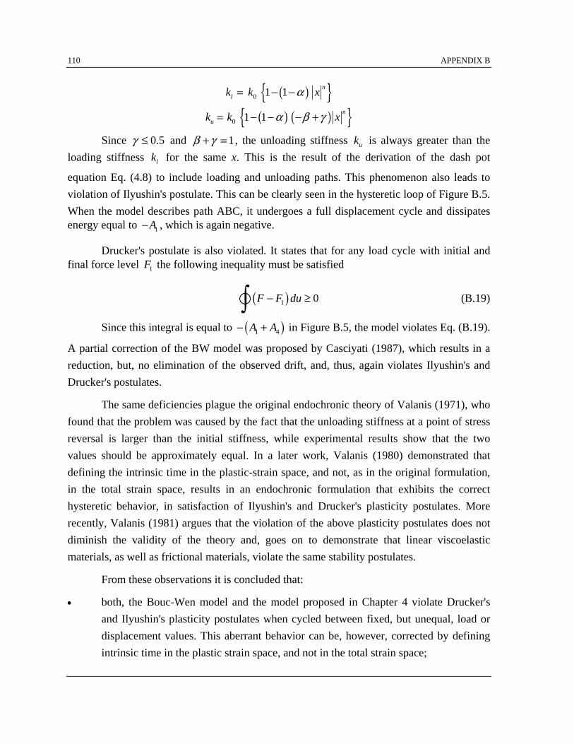
110 APPENDIX B

( ){ }( ) ( ){ }

0

0

1 1

1 1

nl

nu

k k x

k k x

a

a b g

= - -

= - - - +

Since 0.5g £ and 1b g+ = , the unloading stiffness uk is always greater than theloading stiffness lk for the same x. This is the result of the derivation of the dash pot

equation Eq. (4.8) to include loading and unloading paths. This phenomenon also leads toviolation of Ilyushin's postulate. This can be clearly seen in the hysteretic loop of Figure B.5.When the model describes path ABC, it undergoes a full displacement cycle and dissipatesenergy equal to 1A- , which is again negative.

Drucker's postulate is also violated. It states that for any load cycle with initial andfinal force level 1F the following inequality must be satisfied

( )1 0F F du- ≥Ú (B.19)

Since this integral is equal to ( )1 4A A- + in Figure B.5, the model violates Eq. (B.19).

A partial correction of the BW model was proposed by Casciyati (1987), which results in areduction, but, no elimination of the observed drift, and, thus, again violates Ilyushin's andDrucker's postulates.

The same deficiencies plague the original endochronic theory of Valanis (1971), whofound that the problem was caused by the fact that the unloading stiffness at a point of stressreversal is larger than the initial stiffness, while experimental results show that the twovalues should be approximately equal. In a later work, Valanis (1980) demonstrated thatdefining the intrinsic time in the plastic-strain space, and not, as in the original formulation,in the total strain space, results in an endochronic formulation that exhibits the correcthysteretic behavior, in satisfaction of Ilyushin's and Drucker's plasticity postulates. Morerecently, Valanis (1981) argues that the violation of the above plasticity postulates does notdiminish the validity of the theory and, goes on to demonstrate that linear viscoelasticmaterials, as well as frictional materials, violate the same stability postulates.

From these observations it is concluded that:

• both, the Bouc-Wen model and the model proposed in Chapter 4 violate Drucker'sand Ilyushin's plasticity postulates when cycled between fixed, but unequal, load ordisplacement values. This aberrant behavior can be, however, corrected by definingintrinsic time in the plastic strain space, and not in the total strain space;

APPENDIX B 111

• the two postulates do not represent strict physical or thermodynamical requirements,and other widely used mechanical models exhibit the same behavior;

• the refinement of the model in Chapter 4 to satisfy the two postulates in accordancewith Valanis' recent proposals is beyond the scope of this study. Moreover, extensivenumerical simulations with the model have shown that its numerical stability andaccuracy is not affected by the violation of Ilyushin's and Drucker's postulates.