Electronic copy available at: http://ssrn.com/abstract=1550253

A Bayesian Approach forCapturing Daily Heterogeneity

in Intra-Daily Durations Time Series:the Mixed Autoregressive Conditional Duration Model

Christian T. Brownlees ∗ Marina Vannucci †

February 2010

Abstract

Standard intra-daily duration analysis assumes that diurnally adjusted durations re-vert around the same mean level each day. Such an assumption may be too stringent inpractice as duration time series often exhibit evidence of different mean reversion levelson different days. These patterns arise as the consequence of trading habits and economicshocks affecting the high frequency level of market activity. For instance, trading canon average be slower on days following holidays and can be faster on macro announce-ments days. In this work we propose a novel three component model that consists ofan autoregressive daily random effect, a semiparametric time-of-day effect and a intra-daily dynamic component. We name this the Mixed Autoregressive Conditional Duration(Mixed ACD) model. The random effect component captures heterogeneity in daily meanreversal and can be interpreted as daily expected duration. A Bayesian formulation ofthe model allows for the joint estimation of model parameters using MCMC techniques.The empirical application to a set of widely traded US tickers shows that the expecteddaily duration has strong posterior evidence of positive dependence. We also find thatthe degree of dependence and dispersion is higher in periods of higher financial distress.

Keywords: Financial Durations, ACD, MCMC

JEL: C11, C14, C22

∗Department of Finance, Stern School of Business, New York University, e-mail: ctb@stern.nyu.edu†Department of Statistics, Rice University, e-mail: marina@rice.edu

We would like to thank Robert Almgreen, Giorgio Calzolari, Fabrizio Cipollini, Rohit Deo, Rob Engle, FarhangFarazmand, Giampiero M. Gallo, Eric Ghysels, Joel Hasbrouck, Bryan Kelly, Dennis Kristensen, AlbertMenkveld, Lea Petrella, Jose Gonzalo Rangel, Richard Spady and conference participants at the “GreaterNY Metropolitan Area Econometrics Colloquium” (Princeton, USA, 6 December, 2008) and the “Humboldt-Copenhagen Conference 2009” (Berlin, Germany, 20-21 March, 2009) for comments. All mistakes are ours.

1

Electronic copy available at: http://ssrn.com/abstract=1550253

1 Introduction

Intra-daily financial duration analysis has been an active field of research since the seminal con-tribution of Engle & Russell (1998). Durations time series are defined as waiting times betweenmarket events of interest (transactions, price changes above or below a given threshold, execu-tion of a given amount of shares, etc.). The main documented stylized facts of these types ofseries are diurnal periodicity and duration clustering. These empirical regularities have initiallymotivated models that decompose expected duration in a semiparametric diurnal componentand a dynamic component. Among other directions, a significant proportion of subsequentresearch has focused on providing more sophisticated descriptions of the duration dynamics(e.g. Bauwens & Giot (2000), Zhang, Russell & Tsay (2001), Fernandes & Grammig (2006))and more realistic assumptions on the (standardized) duration distribution (e.g. Grammig &Maurer (2000)).

Standard duration time series models assume that duration dynamics are the same on eachday. This in practice may be too much of a stringent assumption. We claim that intra-dailyduration series exhibit clustering around different levels on different days. We interpret thisas an effect of low frequency events affecting the high frequency level of market activity. Forexample, trading can on average be slower on days following holidays and can be faster on macroannouncements days. However, explicitly modeling the impact of lower frequency events onthe duration dynamics poses several challenges. For instance, it is not obvious which holidaysand news announcements should be included in the specification. Furthermore, allowing formany different types of events may lead to expensively parametrized models. To avoid thesecomplications, while still allowing for different regimes of daily activity, we resort to randomeffect modeling. We propose a novel Mixed Autoregressive Conditional Duration (Mixed ACD)model which builds up on the classic approach by adding a daily random effect to a modelconsisting of a semiparametric diurnal component and a dynamic component. The latent factorcaptures heterogeneity and allows for different mean reversion levels of intra-daily durationsdynamics on different days. Such unobservable variables can be interpreted as daily expectedduration. The random effect is specified as an autoregressive process to accommodate for inter-daily dependence in expected duration. Put in a different way, our latent factor approachcan be seen as an alternative device to capture long range dependence which several authorshave documented in financial durations time series (inter alia Jasiak (1998), Chen & Deo(2006), Fernandes, Medeiros & Veiga (2006)). In this respect our model is closely related to theSpline-GARCH (Engle & Rangel (2008)) where a semiparametric smoother (which is functionof calendar time) is used to capture low frequency components in volatility.

The inclusion of latent dynamic factors to the duration specification makes the likelihoodof the model intractable. On the other hand, a Bayesian formulation of the model allows forinference via MCMC techniques. We propose an MCMC procedure which exploits the specialstructure of the specification: the Mixed ACD model components have either ARMA or GLMrepresentations for which effective proposals to be used in Metropolis steps are available. TheBayesian MCMC procedure we develop estimates all the components of the model simulta-neously rather than relying on the customary two-step estimation procedure. Moreover, theamount of smoothing to be imposed in the semiparametric estimate of the diurnal component isembedded in the Bayesian estimation problem and is estimated together with the other modelparameters.

The empirical study focuses on a set of widely traded US tickers across different sampleperiods characterized by different levels of volatility. For the great majority of our series, we

2

show that the residuals of the standard Autoregressive Conditional Duration (ACD) (Engle& Russell (1998)) exhibit evidence of daily heterogeneity and low frequency dependence. Onthe other hand, the Mixed ACD captures such features providing a better characterizationof the duration dynamics. The estimation results of the expected daily duration componentreveal that there is strong evidence of positive intra-daily dependence and that the degree ofdependence and dispersion is higher in periods of higher financial distress.

The main contributions of this work are both methodological and empirical. From a method-ological perspective we propose a new model for financial durations and a Bayesian MCMCsampling procedure for inference which blends approaches stemming from the nonlinear timeseries and semiparametric literature. Moreover, an appealing feature of the Bayesian formu-lation of the problem is that all model parameters as well as smoothing parameters of thesemiparametric components are simultaneously estimated, as opposed to the traditional multi–step estimation approach typically used in the literature. The empirical study unveils empiricalfeatures of a moderately large set of tickers across sample periods that have not been exten-sively studied yet. For instance, we analyse duration dynamics during the beginning of thecredit crunch crisis in summer 2007.

Several contributions relate to our work. Recent developments in the analysis of irregularlyspaced data include Bauwens, Giot, Grammig & Veredas (2004), Fernandes & Grammig (2005),Bauwens & Hautsch (2006). The analysis of long range dependence in duration dynamics hasrecently been addressed in Deo, Hsieh & Hurvich (2007) and Deo, Hurvich, Soulier & Wang(2010) from a long memory perspective. The relationship between financial time series dynam-ics at daily and intra-daily frequencies has been addressed in the volatility and volume modelingliterature in the work of Engle, Sokalska & Chanda (2005), Ghysels, Santa-Clara & Valkanov(2006) and Brownlees, Cipollini & Gallo (2010) for instance. Other authors have consideredintra-daily dynamic models with latent dynamic components in the financial econometric liter-ature, like, for instance, Hautsch (2008). However, our work differs from previous work, in thatwe use latent dynamics to capture low frequency heterogeneity and clustering in the data. Themethodology presented in this work is also related to the volatility models proposed in Engle& Rangel (2008) and Brownlees & Gallo (2008), where a semiparametric component is used tocapture volatility trends. The semiparametric Bayesian approach we employ builds up from thework of Eilers & Marx (1996) who propose a Generalized Additive Models (GAM) formulationbased on B-splines; and Brezger & Lang (2006) who develop Bayesian MCMC inferential pro-cedures based on smoothness priors. Similar approaches have been employed in the Bayesianeconometric literature in the work of Koop & Poirer (2004) and Pangiotelis & Smith (2008)for instance. The Mixed ACD Bayesian analysis is also closely related to the Bayesian analysisof GARCH models, which has been addressed among others by Geweke (1989), Kleinbergen &Van Dijk (1993), Bauwens & Lubrano (1998) and Nakatsuma (2000).

Section 2 describes the datasets used in this work. Section 3 introduces the Mixed ACDand discusses Bayesian inference based on MCMC techniques. Section 4 shows the results of apreliminary ACD analysis and presents the results of an application of the Mixed ACD on ourdatasets. Section 5 contains concluding remarks.

2 Data

Our empirical study consists of the analysis of intra-daily trade durations for 33 US tickers inthe summers (that is July, August and September) of 2002, 2005 and 2007. Table 1 reports

3

(a)

(b)

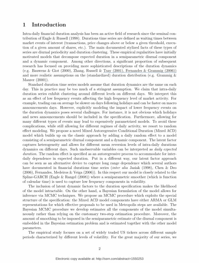
Figure 1: SPY trade durations in summer 2007: (a) full sample and (b) 1 week subsample timeseries plots.

4

Ticker Company Ticker Company Ticker Company

AA Alcoa HD Home Depot MRK MerckAIG American International Group HON Honeywell International MSFT Microsoft CorporationAXP American Express HPQ Hewlett-Packard PFE PfizerBA Boeing IBM IBM PG Procter & GambleC Citigroup INTC Intel QQQQ PowerShares QQQ Trust ETFCAT Caterpillar JNJ Johnson & Johnson SPY SPDR Trust ETFDD DuPont JPM JPMorgan Chase T AT&TDIA Diamonds Trust ETF KO Coca-Cola UTX United Technologies CorporationDIS Walt Disney MCD McDonald’s VZ Verizon CommunicationsGE General Electric MMM 3M WMT WalmartGM General Motors MO Altria Group XOM ExxonMobil

Table 1: Tickers and Company Names.

Ticker 2002 2005 2007 Ticker 2002 2005 2007 Ticker 2002 2005 2007

AA 32 63 662 HD 111 108 651 MRK 54 97 424AIG 46 80 531 HON 30 47 220 MSFT 796 797 1001AXP 42 52 355 HPQ 0 0 0 PFE 107 168 673BA 42 61 283 IBM 86 88 335 PG 44 80 432C 119 132 1162 INTC 755 773 1076 QQQQ 615 570 851CAT 24 66 322 JNJ 65 80 431 SPY 328 936 2988DD 33 68 252 JPM 76 90 807 T 45 33 662DIA 184 97 344 KO 40 69 340 UTX 28 55 239DIS 61 71 339 MCD 41 72 317 VZ 61 77 409GE 190 174 933 MO 71 73 391 WMT 72 133 592GM 46 63 499 MMM 36 55 187 XOM 78 174 1102

Table 2: List of the trade durations threshold values c. For each ticker and sample period, thetable reports the number of c trades that need to be executed to define an aggregated tradeduration.

the full list of tickers used in this work: the set contains the ETFs of the S&P500 (SPY), DowJones Industrial Average (DIA) and Nasdaq (QQQQ) indices as well as other 30 widely tradedUS stocks which either are or have been components of the Dow Jones Industrial Average. Thesample periods considered contain both episodes of high volatility like summer 2002 and 2007characterized by, respectively, the dot–com bubble burst and the credit crunch crisis; and lowvolatility like summer 2005. We define trade durations as units of time needed to observe ctrades being executed. For each ticker/sample period c is chosen as to have approximately 100observations per day, leading to samples of approximately 6000 observations. We use aggregateddurations to obtain datasets of approximately the same size and to ease the numerical burdenof the analysis. Note however that this implies losing the ability of interpreting the averageduration level of the series across different samples as all series have roughly the same mean.Table 2 reports the chosen c values picked in this study. The threshold values c steadily increaseacross sample periods. This is a consequence of the surge in the level of trading generated bythe advent of automated order execution systems (algorithmic trading cf. Chordia, Roll &Subrahmanyam (2008), Brownlees et al. (2010)). The empirical analysis we present has alsobeen performed on price durations (i.e. waiting time of a price change above or below a giventhreshold) and volume durations (i.e. waiting time for a certain amount of volumes beenexchanged). For these other datasets the empirical results are essentially the same and hencewe decided to report trade durations results only. The data used in this work are extractedfrom the NYSE-TAQ database (see Brownlees & Gallo (2006) for details on the data handling).

Let us begin with some anecdotal evidence which aims at highlighting the connectionsbetween specific low frequency events and high frequency level of trading. We will later present

5

2002 2005 2007s ρtick

1 ρtick1/2 day

ρtick1 day s ρtick

1 ρtick1/2 day

ρtick1 day s ρtick

1 ρtick1/2 day

ρtick1 day

AA 0.69 0.37 0.12 0.05 0.95 0.60 0.19 0.15 2.09 0.75 0.39 0.35AIG 0.99 0.47 0.24 0.14 1.00 0.59 0.24 0.19 1.65 0.68 0.41 0.33AXP 0.60 0.40 0.13 0.07 0.85 0.52 0.14 0.08 2.17 0.68 0.37 0.26BA 0.92 0.55 0.24 0.18 1.04 0.56 0.24 0.20 1.72 0.71 0.35 0.30C 1.13 0.56 0.36 0.31 0.74 0.56 0.20 0.15 2.14 0.77 0.50 0.39CAT 0.61 0.33 0.09 0.05 1.13 0.64 0.33 0.25 1.72 0.71 0.39 0.30DD 0.79 0.45 0.20 0.15 0.80 0.54 0.25 0.17 1.66 0.67 0.34 0.30DIA 3.12 0.69 0.32 0.22 1.49 0.52 0.12 0.11 2.48 0.69 0.42 0.35DIS 0.87 0.55 0.30 0.23 0.89 0.54 0.26 0.17 1.55 0.61 0.35 0.31GE 1.17 0.65 0.33 0.29 0.60 0.47 0.10 0.07 1.49 0.66 0.36 0.29GM 0.79 0.50 0.13 0.15 1.07 0.60 0.19 0.12 2.03 0.71 0.38 0.32HD 1.47 0.71 0.42 0.40 0.89 0.61 0.20 0.16 1.62 0.65 0.26 0.20HPQ 0.67 0.48 0.25 0.24 0.78 0.61 0.36 0.30 0.73 0.67 0.35 0.30HON 0.88 0.53 0.32 0.22 0.76 0.43 0.15 0.12 1.27 0.58 0.27 0.24INTC 1.16 0.67 0.28 0.25 0.96 0.50 0.16 0.10 1.20 0.57 0.19 0.13IBM 0.84 0.59 0.26 0.20 0.93 0.57 0.24 0.21 1.33 0.64 0.29 0.26JNJ 1.32 0.74 0.56 0.53 0.65 0.47 0.14 0.09 1.35 0.63 0.34 0.27JPM 1.05 0.66 0.33 0.28 0.66 0.47 0.10 0.08 2.21 0.77 0.47 0.40KO 0.57 0.34 0.13 0.14 0.63 0.44 0.09 0.04 1.46 0.61 0.31 0.22MCD 1.20 0.64 0.44 0.40 0.96 0.62 0.25 0.14 1.76 0.68 0.38 0.35MMM 0.80 0.46 0.18 0.15 0.66 0.47 0.10 0.09 1.59 0.64 0.31 0.25MO 1.09 0.67 0.37 0.25 1.01 0.62 0.31 0.27 1.18 0.61 0.24 0.21MRK 1.06 0.55 0.34 0.29 1.18 0.75 0.54 0.50 1.46 0.65 0.34 0.29MSFT 1.18 0.69 0.33 0.28 1.10 0.51 0.22 0.19 1.24 0.57 0.26 0.19PFE 0.95 0.64 0.38 0.34 0.79 0.52 0.14 0.09 1.10 0.56 0.28 0.19PG 0.58 0.41 0.14 0.11 0.64 0.47 0.09 0.07 1.24 0.61 0.33 0.26QQQQ 1.39 0.70 0.40 0.37 0.82 0.52 0.04 0.01 2.07 0.69 0.37 0.28SPY 1.04 0.62 0.17 0.11 0.95 0.56 0.11 0.04 2.11 0.75 0.45 0.33T 0.76 0.42 0.20 0.17 0.59 0.37 0.00 0.01 1.13 0.59 0.28 0.23UTX 0.66 0.36 0.09 0.06 0.73 0.46 0.08 0.08 1.42 0.63 0.29 0.24VZ 0.73 0.47 0.22 0.17 0.59 0.45 0.12 0.10 1.26 0.59 0.28 0.26WMT 0.94 0.38 0.20 0.15 1.43 0.74 0.47 0.43 1.47 0.66 0.27 0.19XOM 1.06 0.62 0.38 0.32 0.73 0.58 0.15 0.05 1.36 0.68 0.41 0.34Q10 0.61 0.37 0.13 0.07 0.62 0.45 0.09 0.04 1.17 0.58 0.26 0.19Median 0.94 0.55 0.26 0.22 0.85 0.54 0.16 0.12 1.49 0.66 0.34 0.28Q90 1.33 0.69 0.40 0.38 1.14 0.62 0.34 0.28 2.15 0.75 0.43 0.35

Table 3: Duration descriptive statistics. Standard deviation of the average daily duration sand adjusted durations autocorrelation at lag 1 (ρtick

1 ), lag 50 (ρtick1/2 day) and lag 100 (ρtick

1 day) foreach ticker and sample period.

6

a more rigorous analysis on the evidence of neglected low frequency components in standardACD specifications in Section 4. The visual inspection of the duration time series suggests thattrading habits and economic shocks affect the high frequency level of market activity and thatthese shocks cluster. This is a relatively not surprising fact given the vast empirical evidencereported by the ARCH literature. Figure 2 displays the full sample as well as one week oftrade durations of the SPY ticker in summer 2007. Durations are plotted on a transformedcalendar time-scale in such a way that each unit interval contains the observations of onetrading day. For instance, the interval (2, 3) contains the data of the 3rd trading day in thesample, with 2 corresponding to 9:30 and 3 to 16:00 (note that the mapping keeps the seriesirregularly spaced). The series clearly exhibits the well documented stylized facts of this typeof data: diurnal periodicity and duration clustering. However, visual inspection of the graphsalso suggests the presence of daily clusters of high/low trading activity. For instance, tradingis much slower on the 3rd and 4th day in the sample (first shaded area from the left in thegraph), with day 4 containing the longest duration in the sample. These days are Thursday5th and Friday 6th of July, the first two trading days after Independence Day, a U.S.A. federalholiday. There is a large cluster of quick trading days in between, roughly, the 15th and 35th

day (second shaded from the left area). The period corresponds to the end of July/first half ofAugust when the first news about the incoming credit crunch crisis started to leak. On Friday20th of July Federal Reserve chairman Ben Bernanke warned about severe losses due to theUS sub-prime lending market crisis and on Thursday 9th August 2007 the inability of BNPParibas to evaluate its assets because of an evaporation of liquidity followed by a halt on thewithdrawals from some of its investment funds is recognized as the first clear sign of the creditcrunch. Lastly, there is quick trading on the 55th and 56th day (third shaded area from the left).These days are Monday 17th of August and that is when the former U.S. Fed Chairman AlanGreenspan warned about “large double digits declines” in home values followed by Tuesday18th when the U.S. Fed cut the interest rate by half a point.

Similar insights can be gathered by the inspection of the series of full set of tickers across thedifferent sample periods. We synthesize the evidence of lower frequency dynamics by showingthat the autocorrelation function of the adjusted durations1exhibits evidence of long range(cf. Deo et al. (2007)). Table 3 contains the autocorrelation of the adjusted durations atlag 1, lag 50 (corresponding to approximately a half day lag) and lag 100 (corresponding toapproximately a day lag) for each dataset. We use the expression “adjusted durations” as shortnotation for “diurnally adjusted durations” that is durations divided by an estimate of thediurnal component. For the vast majority of cases, the autocorrelations are all significant andslowly decaying. Moreover, the degree of dependence is stronger in 2007, followed by 2002 and2005.

3 The Mixed Autoregressive Conditional Duration Model

3.1 Model

The anecdotal evidence of Section 2 hints that a high frequency model for durations with adynamic daily frequency component ought to provide a more realistic description of the data.The Mixed ACD is a generalization of the standard ACD methodology obtained by including adaily random effect to capture heterogeneity in daily mean reversion in the specification. Let τt i(t = 1, ..., T and i = 1, ..., It) denote the series of arrival times of some intra-daily market event

7

of interest, with the t i subscript referring to the ith arrival time on day t. The correspondingseries of durations is given by xt i = τt i − τt i−1. The model is defined as

xt i = µt i εt i εt i ∼ Exp(1) (1)

where µt i is the expected duration of xt i and εt i is an iid exponetial innovation with unitexpected value (for a discussion on alternative baseline distribution specifications see Hautsch(2004)). The expected duration µt i is assumed to be given by the product of three components

µt i = ηt φt i ψt i . (2)

The first component ηt is an exponentiated autoregressive daily random effect component cap-turing daily heterogeneity in mean reversal and is defined as

ηt = exp {ut}, ut|ut−1 ∼ N(ρut−1, σ2u). (3)

The component φt i is a semiparametric diurnal time of day effect (constrained to be 1 onaverage) and is defined as

φt i = exp { f(τt i−1) } = exp

{K∑k=1

γk Bk ( τt i−1 )

}, (4)

with Bk(·), k = 1, ..., K, a cubic B-splines linear basis expansion with respect to a set of equallyspaced knots {τ (1), ..., τ (K)}. Finally, ψt i is a intra-daily dynamic ACD process capturing intra-daily duration clustering and whose dynamics evolve according to

ψt i = ω + α

(xt i−1

ηt φt i

)+ βψt i−1. (5)

In what follows, we refer to the sum of the parameters α and β as the intra-daily persistence, inthat this quantity governs the degree of mean reversion of the intra-daily dynamic component.

The standard ACD model of Engle & Russell (1998) is nested in the Mixed ACD as alimiting case when the variance of the random effect shrinks to zero. The specification also hassome analogies with regime-switching type models, in that the Mixed ACD has a (deterministic)regime switch in the mean reversion level each day. As opposed to regime-switching modelshowever, where a small number of regimes is typically chosen, the Mixed ACD allows for adifferent regime on each day. Also note that the autoregressive structure of daily expectedduration allows one to compute multi day ahead predictions. We resort to a low rank smootherbased on B–splines in that this type of basis functions have good numerical properties and allowto easily impose shape constraints which are useful for both classical and Bayesian estimation.

In the classical framework, the specification described by Equations (1) to (5) would typ-ically be estimated by some penalized maximum likelihood procedure, with the penalizationdelivering shrinkage of the semiparametric component coefficients (as customary in the smooth-ing literature). The objective function of the model would be given by

Qλ(θ) =

∫ T∑t=1

It∑i=1

log f(xt i|xt i−1, τt i−1, ηt, θ)p(ηt|ηt−1, θ)− λ γ′Pγ

with P being a (positive definite) K × K “penalty” matrix and λ ∈ R+ being a smoothingparameter. Such objective function is intractable due to the multidimensional integrationproblem arising from the presence of the random effects in the specification. Moreover, thechoice of smoothing parameter λ adds another layer of complexity to the estimation problem(cf. Leeb & Potscher (2005)). However, a Bayesian formulation of the problem provides aneffective machinery for estimation and inference.

8

3.2 Priors

We adopt standard prior distributions for the parameters of the Mixed ACD components (cf.Chib & Greenberg (1994), Nakatsuma (2000), Brezger & Lang (2006)). In the empirical appli-cation such distributions will be made sufficiently diffuse over the parameter space.

The priors for the random effects parameters consist of a truncated normal prior for theautoregressive parameter ρ ∝ N(0, σ2

ρ)Icη(ρ), where I denotes the indicator function and cη(·) isthe set of values of ρ where the process is stationary (i.e. |ρ| < 1); and an Inverse Gamma forthe variance of the random effect σ2

u ∼ IG(au, bu).Following Eilers & Marx (1996) and Brezger & Lang (2006), the prior for the semiparametric

component exploit specific properties of the B-splines that allow to control the smoothness ofthe spline functions. Specifically, the derivatives (of order d) of the spline function

∑γkBk(·)

are a linear combination of the finite differences (of order d) of adjacent B-splines coefficients γ.This property allows to control the spline smoothness by constraining the finite differences ofthe B-splines coefficients. We assume that adjacent γ coefficients follow a third order randomwalk

∇3γk = uk γ j = 4, ..., K

with γkc ∝ const for k = 1, 2, 3 and that the innovation term of the random walk is normaluk γ ∼ N(0, σ2

γ) with variance having an Inverse Gamma prior σ2γ ∝ IG(aγ, bγ). These pri-

ors shrink the estimated diurnal time-of-day effect towards a quadratic polynomial with theamount of shrinkage controlled by σ2

γ, which in fact can be interpreted as the reciprocal of theregularization parameter λ in the (classical) penalized maximum likelihood framework. Suchsmoothness prior is justified by the well documented mound shaped pattern in trading activityexhibited by NYSE duration series.

Finally, the dynamic component parameters ω, α and β have a truncated normal prior ωαβ

∝ N

0.3 x0.20.5

, σ2ψI

Icψ(ω,α,β)

where x is the average duration in the sample and cψ(·, ·, ·) denotes the set over which expectedintra-daily durations are finite, positive and stationary (i.e. ω > 0, α + β < 1, α > 0 andβ ≥ 0). The prior for (α, β) is centered around (0.2, 0.5), implying that the prior intra-dailypersistence α+β is set to be lower than the typical ACD estimates. We make this choice in thatit is expected that part of intra-daily persistence is absorbed by the daily random component.The prior for ω ensures that the mean of the data and of the expected prior intra-daily dynamiccomponent match.

3.3 Posterior Inference

Le θ denote the vector of model parameters and random effects (ρ, u1, ..., uT , σ2u, γ1, ..., γK , ω, α, β).

MCMC techniques allow us to construct approximate samples from the posterior distributionof the model parameters and random effects given by the otherwise analytically intractable

p(θ|x) ∝ `(x|u, θ) p(u|ρ, σ2u)p(ρ)p(σ2

u) p(γ|τ 2)p(τ 2) p(ω)p(α)p(β),

where `(·) is the likelihood function and p(·) denotes the prior of the model parameters anddistribution of the random effects. We generate samples using a Metropolis Hastings (MH)

9

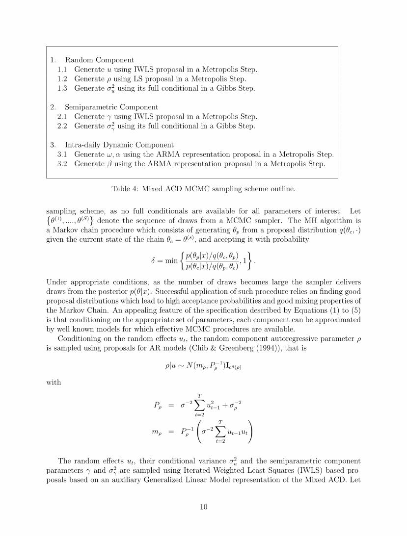
1. Random Component1.1 Generate u using IWLS proposal in a Metropolis Step.1.2 Generate ρ using LS proposal in a Metropolis Step.1.3 Generate σ2

u using its full conditional in a Gibbs Step.

2. Semiparametric Component2.1 Generate γ using IWLS proposal in a Metropolis Step.2.2 Generate σ2

γ using its full conditional in a Gibbs Step.

3. Intra-daily Dynamic Component3.1 Generate ω, α using the ARMA representation proposal in a Metropolis Step.3.2 Generate β using the ARMA representation proposal in a Metropolis Step.

Table 4: Mixed ACD MCMC sampling scheme outline.

sampling scheme, as no full conditionals are available for all parameters of interest. Let{θ(1), ...., θ(S)

}denote the sequence of draws from a MCMC sampler. The MH algorithm is

a Markov chain procedure which consists of generating θp from a proposal distribution q(θc, ·)given the current state of the chain θc = θ(s), and accepting it with probability

δ = min

{p(θp|x)/q(θc, θp)

p(θc|x)/q(θp, θc), 1

}.

Under appropriate conditions, as the number of draws becomes large the sampler deliversdraws from the posterior p(θ|x). Successful application of such procedure relies on finding goodproposal distributions which lead to high acceptance probabilities and good mixing properties ofthe Markov Chain. An appealing feature of the specification described by Equations (1) to (5)is that conditioning on the appropriate set of parameters, each component can be approximatedby well known models for which effective MCMC procedures are available.

Conditioning on the random effects ut, the random component autoregressive parameter ρis sampled using proposals for AR models (Chib & Greenberg (1994)), that is

ρ|u ∼ N(mρ, P−1ρ )Icη(ρ)

with

Pρ = σ−2

T∑t=2

u2t−1 + σ−2

ρ

mρ = P−1ρ

(σ−2

T∑t=2

ut−1ut

)

The random effects ut, their conditional variance σ2u and the semiparametric component

parameters γ and σ2γ are sampled using Iterated Weighted Least Squares (IWLS) based pro-

posals based on an auxiliary Generalized Linear Model representation of the Mixed ACD. Let

10

xt i denote the duration adjusted from the intra-daily duration dynamics, that is xt i/ψt i. TheAuxiliary GLM is

xt i ∼ Exp(µt i), (6)

the mean µt i is modeled as

log( µt i ) = ζt i

= ut + f(τt i) (7)

= Z ′t i u+B′t i γ

where ζt i is the so called linear predictor, Z ′t i is the (t i)–th row of the matrix of daily dummyindicators and B′t i is the (t i)–th row of the matrix of linear basis expansion in τt i. The modeldescribed by Equations (6) and (7) is a GLM with exponential response and log link. Weillustrate how such representation is used for the semiparametric component parameters only.The other parameters follows similar steps. The proposal for the B-spline coefficients γ is amultivariate normal

γc|x, ψ, u, σ2u, σ

2γ ∼ N(mγ, P

−1γ ),

where mγ and Pγ are respectively the mean and precision matrix from the IWLS representation,namely

Pγ = B′B +1

σ2γ

K

mγ = P−1γ B′ (x(γc)− ζ−γ),

where σ−2γ K is the covariance matrix associated with random walk process prior, x(γc) is the

vector of working observations ζt i + (xt i − µt i)µ−1t i and ζ−γ is the part of the linear predictor

associated with the other parts of the auxiliary model. The dispersion parameter σ2γ is updated

in a Gibb step. Its full conditional is an Inverse Gamma with parameters a′γ = aγ + rank(K)2

and

b′γ = bγ + γ′Kγ2

.The intra-daily dynamic component parameters (ω, α, β)′ are sampled using proposals based

on the Auxiliary ARMA(1,1) representation of the specification (cf. Engle & Russell (1998))given by

xt i = ω + (α + β)xt i−1 + εt i − βεt i−1 εt i ∼ N(0, ψ2t i),

where xt i = xt i/(ηtφt i) and εt i = xt i − ψt i. The intra-daily dynamic component parametersare obtained using normal proposals of the form

ω, α|x, η, φ, β ∼ N(mω α, P−1ω α)Icψ(α,β) β|x, η, φ, α ∼ N(mβ, P

−1β )Icψ(α,β),

following the approach developed in Chib & Greenberg (1994) and Nakatsuma (2000). Theproposals for ω and α require the computation of several intermediate quantities. Let theauxiliary variables xt i and ιt i be defined using, respectively, the recursions xt i = xt,i + βx(t i)−1

and ιt i = 1 + βι(t i)−1. Moreover, let xt i = xt i − βx(t i)−1 and zt i = (ιt i, x(t i)−1)′. The precisionand mean of the proposal for (ω, α)′ are

Pω α = (X ′ω αΛXω α + Σ−1ω α)

mω α = P−1ω α(X ′ω αΛYω α + Σ−1

ω αµω α).

11

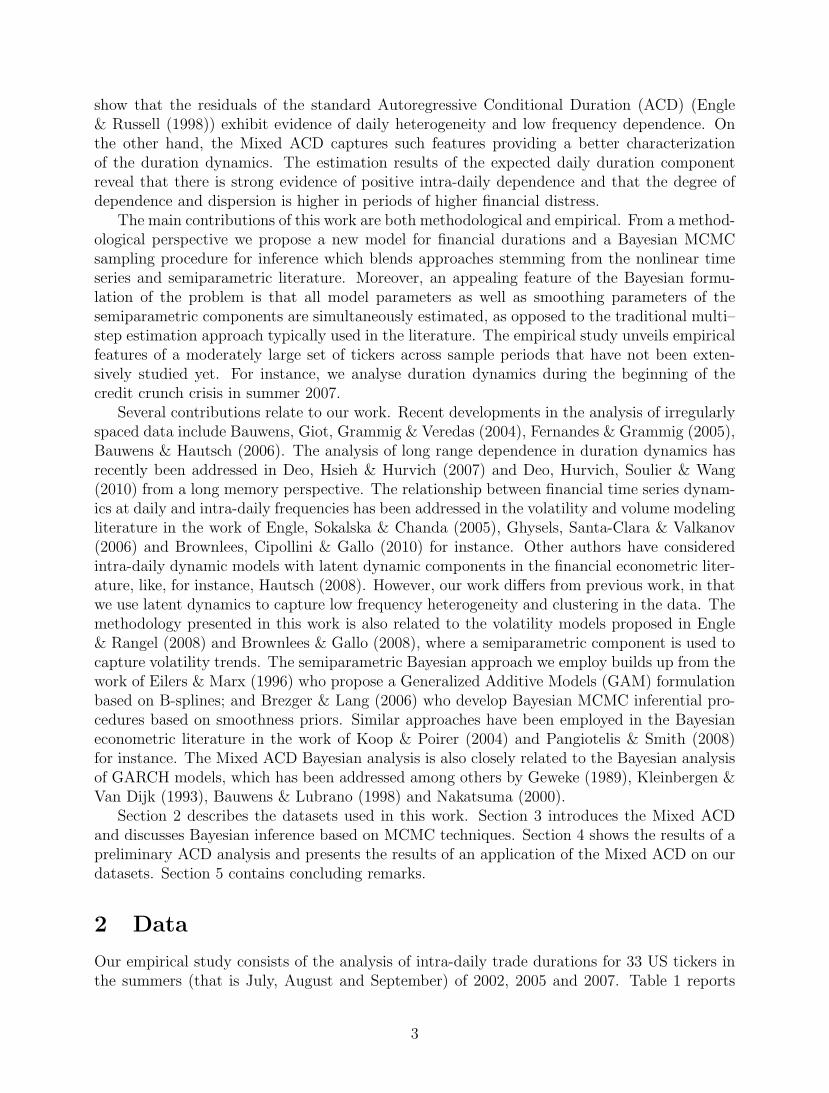
Time Series Autocorrelogram

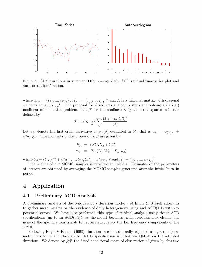
Figure 2: SPY durations in summer 2007: average daily ACD residual time series plot andautocorrelation function.

where Yω α = (x1 1, ..., xT IT )′, Xω α = (z′1 1, ..., z′T IT

)′ and Λ is a diagonal matrix with diagonalelements equal to ψ−2

t i . The proposal for β requires analogous steps and solving a (trivial)nonlinear minimization problem. Let β∗ be the nonlinear weighted least squares estimatordefined by

β∗ = arg maxβ

∑t i

(xt i − ψt i(β))2

ψ2t i

.

Let wt i denote the first order derivative of ψt i(β) evaluated in β∗, that is wt i = ψ(t i)−1 +β∗w(t i)−1. The moments of the proposal for β are given by

Pβ = (X ′βΛXβ + Σ−1β )

mβ = P−1β (X ′βΛYβ + Σ−1

β µβ)

where Yβ = (ε1 1(β∗) + β∗w1 1, ..., εT IT (β∗) + β∗wT IT )′ and Xβ = (w1 1, ..., wT IT )′.The outline of our MCMC sampler is provided in Table 4. Estimates of the parameters

of interest are obtained by averaging the MCMC samples generated after the initial burn–inperiod.

4 Application

4.1 Preliminary ACD Analysis

A preliminary analysis of the residuals of a duration model a la Engle & Russell allows usto gather more insights on the evidence of daily heterogeneity using and ACD(1,1) with ex-ponential errors. We have also performed this type of residual analysis using richer ACDspecifications (up to an ACD(3,3)); as the model becomes richer residuals look cleaner butnone of the specifications is able to capture adequately the low frequency components of theseries.

Following Engle & Russell (1998), durations are first diurnally adjusted using a semipara-metric procedure and then an ACD(1,1) specification is fitted via QMLE on the adjusteddurations. We denote by µacd

t i the fitted conditional mean of observation t i given by this two

12

2002 2005 2007

Pers. ρtick1 day ρdaily

1 DDH Pers. ρtick1 day ρdaily

1 DDH Pers. ρtick1 day ρdaily

1 DDH

AA 0.93 0.00 0.15 *** 0.98 0.00 0.23 1.00 -0.02 0.05AIG 0.95 -0.01 0.46 ** 1.00 0.04 0.60 *** 0.98 -0.01 0.18AXP 0.94 -0.01 0.26 ** 1.00 0.01 0.21 *** 0.96 0.00 0.34 ***BA 1.00 0.02 0.55 *** 1.00 0.00 0.54 *** 0.97 0.00 0.30C 0.98 -0.02 -0.01 0.97 0.01 0.25 0.98 0.00 0.34CAT 0.98 0.01 0.23 0.98 0.00 0.31 0.99 0.02 0.13DD 0.97 0.01 0.28 0.98 0.00 0.24 0.96 0.00 0.50 ***DIA 0.94 -0.01 0.21 *** 0.90 0.02 0.54 *** 0.98 -0.01 0.46DIS 0.95 0.01 0.32 *** 0.97 0.03 0.20 0.97 0.01 0.49GE 0.89 0.03 0.56 *** 0.92 0.00 0.32 *** 0.97 0.02 0.46GM 0.94 0.02 0.38 *** 0.99 0.00 -0.24 0.99 0.01 0.14HD 0.93 0.00 0.54 *** 0.93 0.00 0.52 *** 0.94 0.02 0.39 ***HPQ 0.98 0.02 0.33 0.98 0.01 0.30 0.96 0.01 0.53 ***HON 1.00 0.05 0.30 *** 0.94 0.02 0.59 ** 0.97 0.01 0.35IBM 0.95 0.02 0.28 ** 0.96 0.01 0.37 ** 0.96 0.00 0.31 ***INTC 0.94 0.02 0.59 *** 0.93 0.00 0.36 *** 0.96 -0.02 0.12 ***JNJ 0.99 0.01 -0.24 0.90 0.02 0.40 *** 0.97 0.00 0.31JPM 0.98 -0.02 0.15 0.89 0.02 0.32 *** 0.98 0.01 0.47KO 0.98 0.03 0.40 0.88 0.00 0.13 *** 0.96 -0.02 0.45 **MCD 0.99 0.01 -0.06 0.98 0.00 0.02 0.98 0.00 0.23MMM 1.00 0.02 0.59 *** 0.95 0.03 0.15 ** 0.96 0.01 0.34 ***MO 0.99 0.00 -0.18 0.98 -0.01 0.17 0.98 0.01 0.19MRK 0.98 -0.01 -0.15 *** 1.00 0.00 -0.21 0.96 0.02 0.47 ***MSFT 0.97 0.02 0.60 0.95 0.01 0.52 *** 0.96 0.01 0.23 **PFE 0.98 0.01 -0.04 *** 0.93 0.00 0.38 0.96 0.00 0.35 ***PG 0.92 0.01 0.41 *** 0.97 -0.02 0.23 *** 0.98 0.01 0.38 **QQQQ 0.97 0.00 0.54 *** 0.85 0.00 0.02 *** 1.00 0.06 0.62 ***SPY 0.91 0.01 0.49 *** 0.85 0.00 0.31 *** 0.97 0.00 0.48 **T 0.97 0.01 0.27 0.74 0.00 0.08 *** 0.95 0.01 0.50 ***UTX 0.94 0.00 0.18 *** 0.92 0.02 0.34 *** 0.95 0.01 0.45 ***VZ 0.98 0.02 0.07 0.88 0.02 0.40 *** 0.96 0.03 0.43 ***WMT 0.94 0.01 0.15 *** 0.97 0.01 0.59 0.97 0.01 0.14 **XOM 1.00 0.01 0.67 *** 0.90 0.01 0.17 *** 0.96 0.01 0.62 **Q10 0.93 -0.01 -0.08 0.88 0.00 0.02 0.95 -0.01 0.14Median 0.97 0.01 0.28 0.95 0.00 0.31 0.97 0.01 0.35Q90 1.00 0.02 0.59 1.00 0.02 0.55 0.99 0.02 0.51

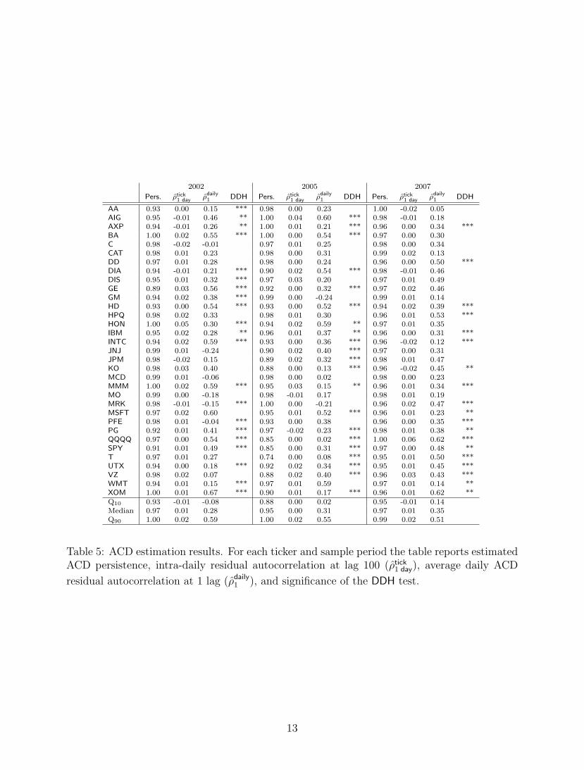
Table 5: ACD estimation results. For each ticker and sample period the table reports estimatedACD persistence, intra-daily residual autocorrelation at lag 100 (ρtick

1 day), average daily ACD

residual autocorrelation at 1 lag (ρdaily1 ), and significance of the DDH test.

13

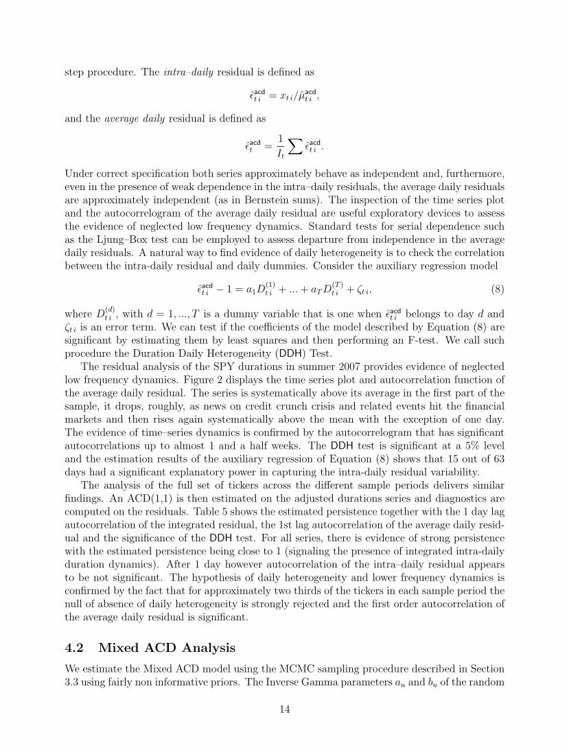
step procedure. The intra–daily residual is defined as

εacdt i = xt i/µacdt i ,

and the average daily residual is defined as

εacdt =1

It

∑εacdt i .

Under correct specification both series approximately behave as independent and, furthermore,even in the presence of weak dependence in the intra–daily residuals, the average daily residualsare approximately independent (as in Bernstein sums). The inspection of the time series plotand the autocorrelogram of the average daily residual are useful exploratory devices to assessthe evidence of neglected low frequency dynamics. Standard tests for serial dependence suchas the Ljung–Box test can be employed to assess departure from independence in the averagedaily residuals. A natural way to find evidence of daily heterogeneity is to check the correlationbetween the intra-daily residual and daily dummies. Consider the auxiliary regression model

εacdt i − 1 = a1D(1)t i + ...+ aTD

(T )t i + ζt i, (8)

where D(d)t i , with d = 1, ..., T is a dummy variable that is one when εacdt i belongs to day d and

ζt i is an error term. We can test if the coefficients of the model described by Equation (8) aresignificant by estimating them by least squares and then performing an F-test. We call suchprocedure the Duration Daily Heterogeneity (DDH) Test.

The residual analysis of the SPY durations in summer 2007 provides evidence of neglectedlow frequency dynamics. Figure 2 displays the time series plot and autocorrelation function ofthe average daily residual. The series is systematically above its average in the first part of thesample, it drops, roughly, as news on credit crunch crisis and related events hit the financialmarkets and then rises again systematically above the mean with the exception of one day.The evidence of time–series dynamics is confirmed by the autocorrelogram that has significantautocorrelations up to almost 1 and a half weeks. The DDH test is significant at a 5% leveland the estimation results of the auxiliary regression of Equation (8) shows that 15 out of 63days had a significant explanatory power in capturing the intra-daily residual variability.

The analysis of the full set of tickers across the different sample periods delivers similarfindings. An ACD(1,1) is then estimated on the adjusted durations series and diagnostics arecomputed on the residuals. Table 5 shows the estimated persistence together with the 1 day lagautocorrelation of the integrated residual, the 1st lag autocorrelation of the average daily resid-ual and the significance of the DDH test. For all series, there is evidence of strong persistencewith the estimated persistence being close to 1 (signaling the presence of integrated intra-dailyduration dynamics). After 1 day however autocorrelation of the intra–daily residual appearsto be not significant. The hypothesis of daily heterogeneity and lower frequency dynamics isconfirmed by the fact that for approximately two thirds of the tickers in each sample period thenull of absence of daily heterogeneity is strongly rejected and the first order autocorrelation ofthe average daily residual is significant.

4.2 Mixed ACD Analysis

We estimate the Mixed ACD model using the MCMC sampling procedure described in Section3.3 using fairly non informative priors. The Inverse Gamma parameters au and bu of the random

14

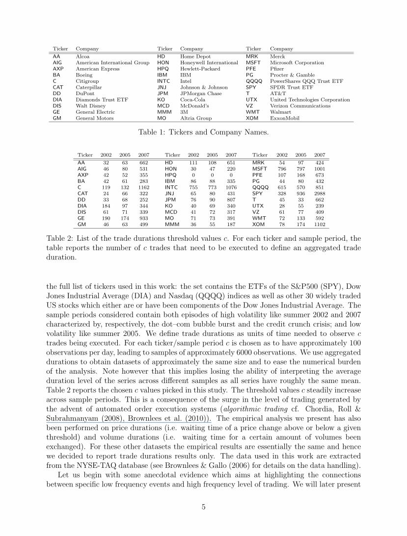
Time Series Autocorrelogram

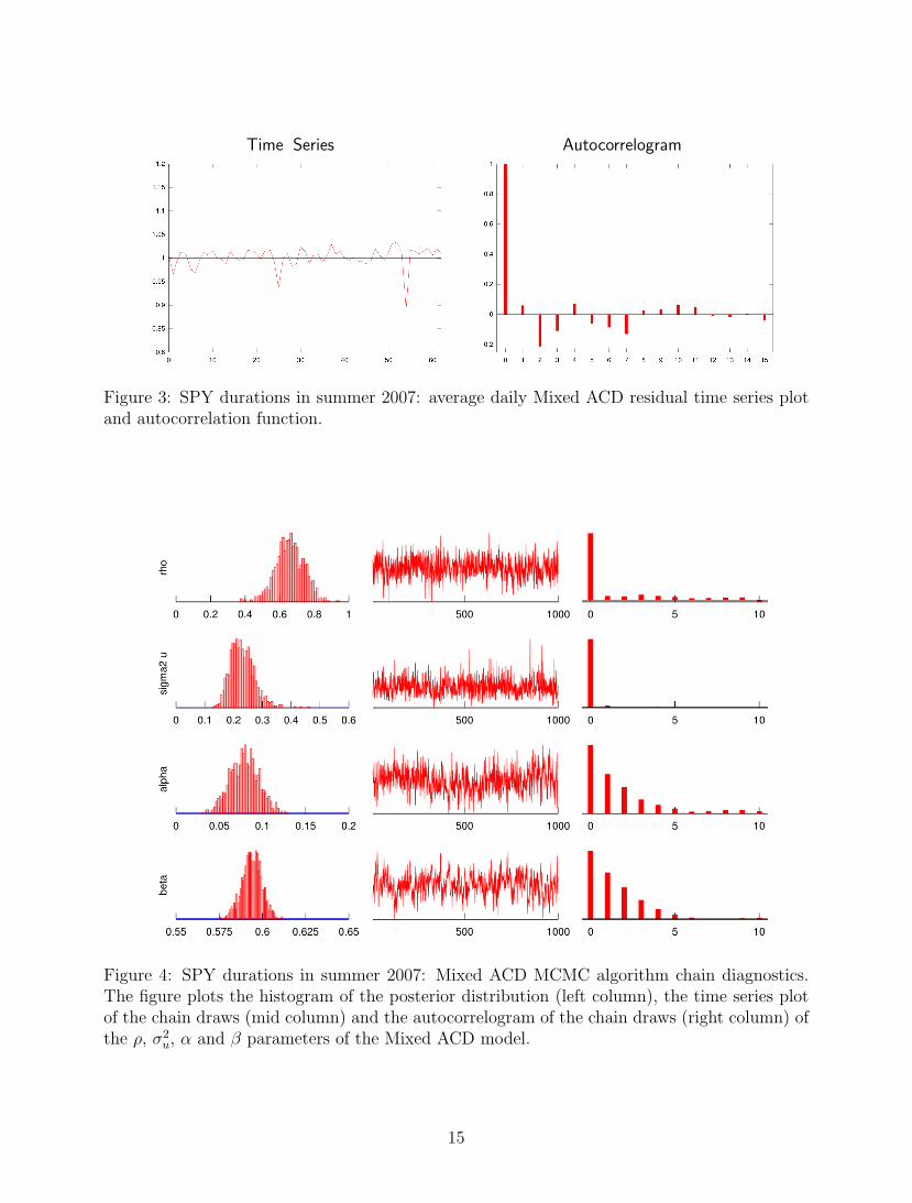
Figure 3: SPY durations in summer 2007: average daily Mixed ACD residual time series plotand autocorrelation function.

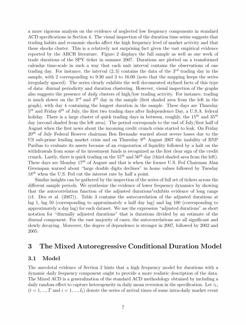
Figure 4: SPY durations in summer 2007: Mixed ACD MCMC algorithm chain diagnostics.The figure plots the histogram of the posterior distribution (left column), the time series plotof the chain draws (mid column) and the autocorrelogram of the chain draws (right column) ofthe ρ, σ2

u, α and β parameters of the Mixed ACD model.

15

Summer 2007

Summer 2002

Figure 5: SPY in summer 2007 and 2002: durations and daily expected duration posteriormean (heavy solid line) with 90% credible bands (light solid line)

16

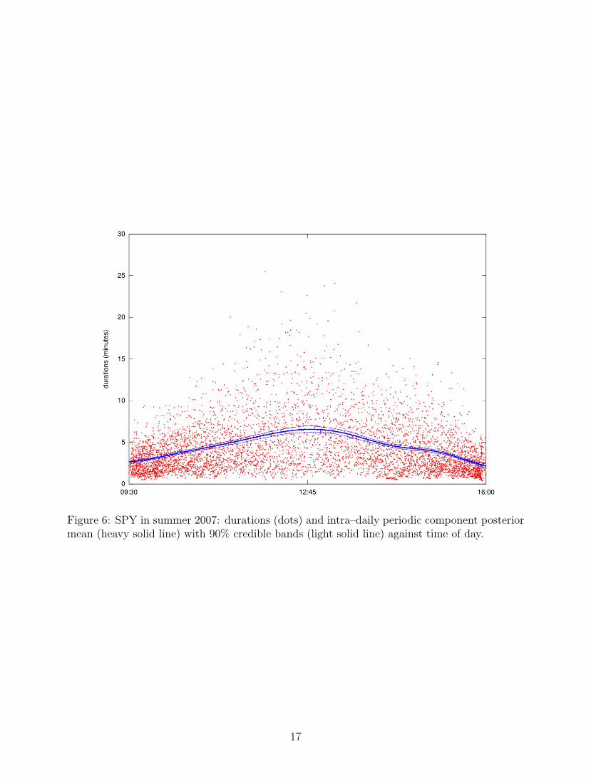
Figure 6: SPY in summer 2007: durations (dots) and intra–daily periodic component posteriormean (heavy solid line) with 90% credible bands (light solid line) against time of day.

17

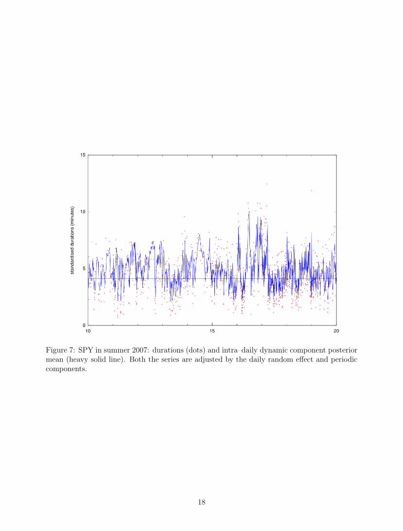
Figure 7: SPY in summer 2007: durations (dots) and intra–daily dynamic component posteriormean (heavy solid line). Both the series are adjusted by the daily random effect and periodiccomponents.

18

2002 2005 2007

pers. ρ σu ρdaily1 pers. ρ σu ρdaily

1 pers. ρ σu ρdaily1

AA 0.75 0.34 0.25 0.01 0.72 0.33 0.30 -0.13 0.75 0.61 0.49 -0.09AIG 0.80 0.48 0.30 0.16 0.71 0.44 0.30 -0.02 0.64 0.62 0.43 0.16AXP 0.85 0.37 0.24 -0.05 0.69 0.34 0.28 -0.25 0.68 0.66 0.46 0.00BA 0.74 0.40 0.30 0.08 0.70 0.46 0.31 0.04 0.68 0.54 0.43 0.00CAT 0.84 0.37 0.25 -0.04 0.77 0.44 0.34 0.14 0.69 0.44 0.45 0.08C 0.57 0.50 0.37 -0.09 0.77 0.37 0.28 0.02 0.75 0.68 0.48 0.00DD 0.84 0.38 0.27 0.03 0.77 0.37 0.28 0.04 0.65 0.67 0.43 -0.02DIA 0.79 0.61 0.47 -0.18 0.52 0.51 0.38 -0.04 0.72 0.73 0.55 0.02DIS 0.47 0.42 0.29 -0.17 0.71 0.38 0.28 -0.12 0.52 0.65 0.41 0.04GE 0.60 0.51 0.34 0.09 0.74 0.37 0.25 -0.25 0.74 0.55 0.38 0.11GM 0.79 0.39 0.26 -0.06 0.72 0.23 0.33 -0.07 0.70 0.54 0.48 -0.04HPQ 0.91 0.43 0.25 0.01 0.82 0.40 0.29 -0.15 0.86 0.44 0.27 0.03HD 0.63 0.64 0.39 -0.07 0.74 0.40 0.29 0.00 0.66 0.50 0.39 0.00HON 0.84 0.31 0.31 0.05 0.64 0.42 0.27 0.10 0.68 0.50 0.36 0.11INTC 0.78 0.50 0.32 -0.02 0.66 0.35 0.30 -0.19 0.78 0.33 0.33 -0.06IBM 0.69 0.41 0.28 0.05 0.71 0.44 0.30 -0.05 0.67 0.50 0.37 0.13JNJ 0.60 0.58 0.41 0.06 0.68 0.39 0.25 -0.08 0.72 0.56 0.37 -0.05JPM 0.66 0.42 0.33 0.01 0.74 0.39 0.25 -0.14 0.73 0.70 0.50 0.02KO 0.81 0.41 0.25 0.11 0.72 0.35 0.25 -0.14 0.56 0.55 0.38 0.13MCD 0.82 0.61 0.35 -0.05 0.70 0.35 0.31 0.13 0.69 0.62 0.44 -0.05MMM 0.81 0.40 0.27 0.10 0.73 0.33 0.25 0.04 0.65 0.55 0.41 0.04MO 0.71 0.33 0.32 0.22 0.75 0.38 0.32 -0.19 0.69 0.45 0.34 0.26MRK 0.54 0.46 0.35 -0.03 0.83 0.56 0.41 0.11 0.61 0.58 0.40 -0.14MSFT 0.82 0.51 0.34 -0.02 0.65 0.47 0.33 -0.28 0.65 0.44 0.35 0.15PFE 0.54 0.43 0.33 -0.24 0.75 0.39 0.27 -0.02 0.65 0.44 0.33 -0.03PG 0.76 0.40 0.25 -0.08 0.76 0.36 0.25 -0.04 0.66 0.55 0.36 0.00QQQQ 0.67 0.66 0.40 -0.05 0.71 0.28 0.27 -0.30 0.72 0.64 0.47 0.05SPY 0.73 0.36 0.30 -0.00 0.67 0.33 0.29 -0.10 0.67 0.66 0.48 0.09T 0.74 0.44 0.28 -0.19 0.50 0.34 0.24 -0.10 0.66 0.51 0.34 0.01UTX 0.83 0.34 0.25 0.06 0.78 0.38 0.26 -0.12 0.68 0.55 0.38 0.05VZ 0.87 0.40 0.26 -0.24 0.69 0.39 0.24 -0.12 0.51 0.52 0.36 -0.05WMT 0.50 0.42 0.30 -0.02 0.75 0.64 0.50 -0.03 0.67 0.43 0.38 0.01XOM 0.69 0.54 0.32 -0.22 0.78 0.34 0.26 -0.08 0.71 0.63 0.38 0.05Q10 0.54 0.35 0.25 -0.19 0.65 0.33 0.25 -0.25 0.60 0.44 0.34 -0.05Median 0.75 0.42 0.30 -0.02 0.72 0.38 0.28 -0.08 0.68 0.55 0.39 0.02Q90 0.85 0.61 0.39 0.10 0.78 0.48 0.35 0.10 0.75 0.67 0.49 0.14

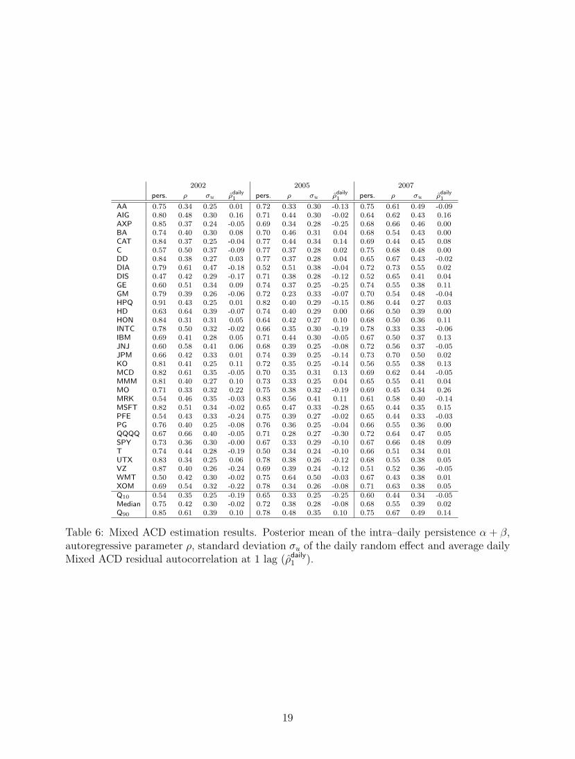
Table 6: Mixed ACD estimation results. Posterior mean of the intra–daily persistence α + β,autoregressive parameter ρ, standard deviation σu of the daily random effect and average dailyMixed ACD residual autocorrelation at 1 lag (ρdaily

1 ).

19

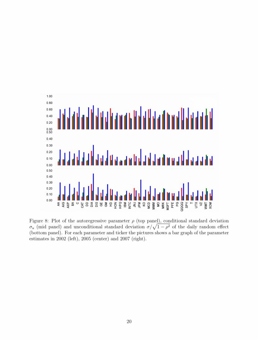
Figure 8: Plot of the autoregressive parameter ρ (top panel), conditional standard deviationσu (mid panel) and unconditional standard deviation σ/

√1− ρ2 of the daily random effect

(bottom panel). For each parameter and ticker the pictures shows a bar graph of the parameterestimates in 2002 (left), 2005 (center) and 2007 (right).

20

effect variance σ2u and aγ and bγ of the semiparametric parameters variance σ2

γ are set to 1 and0.05 respectively. The linear basis expansion of the semiparametric component uses 10 knots.The variances of the dynamic parameters of the models σ2

ρ and σ2ψ are set to 1.

We run 10000 iteration of our MCMC algorithm and discard the first 1000 for burn–in.The chain mixes well and converges to the stationary distribution quickly (≈ 500 iterations).The parameters of the random component and the random effects ut have high acceptanceprobabilities (above 80%) and weakly correlated trace. The semiparametric component param-eters have the lowest acceptance probabilities (above 40%) but correlation in the trace is stilllow. The dynamic component parameters have high acceptance probabilities (above 80%) andmodest correlation in the trace.

We first report detailed evidence for the SPY durations in summer 2007 and then presentgeneral summary statistics for the other series. The Mixed ACD residual diagnostics show aclear improvement over the preliminary ACD analysis of Section 2. Figure 3 displays the timeseries plot and autocorrelogram of the average daily residuals: the time series plot does notexhibit any specific pattern and the autocorrelogram does not signal the evidence of significantdependence. Graphical inspection of the residual time series suggests that the presence of anextreme residual at day 54. Visual inspection of the duration series reveals that this day wascharacterized by very slow trading in the morning followed by a switch to a regime of veryactive trading in the afternoon.

Figure 4 displays chain diagnostics for a subset of the Mixed ACD parameters: the randomcomponent parameters ρ and σ2

u together with the intra-daily dynamic component parametersα and β. The posteriors of ρ and σ2

u are quite disperse over the parameter space. This is due tothe fact that the effective sample size used to estimate these parameters is equal to the numberof days in the sample which is necessarily much smaller than the number of observations.Nevertheless, there is strong posterior evidence of positive dependence with the 90% credibleinterval for ρ being above 0 and its posterior mean being equal to 0.66. The posterior of α andβ are tightly concentrated around their mean values of, respectively, 0.07 and 0.58. which areboth lower than the corresponding MLE estimates of the standard ACD model. The evidence ofnearly integrated inter-durations dynamics disappears with the inclusion of the lower frequencydynamic component.

The fitted random component synthesizes the low frequency dynamics of the series. Figure5 (top graph) shows the time series of posterior mean of the daily expected duration togetherwith 90% credible bands. For instance, during the Independence day week the daily durationcomponent is roughly 10 minutes while during the credit crunch crises it drops to approximately2 minutes. Figure 5 (bottom graph) also reports the same type of plot for the SPY ticker insummer 2002 providing some insights on how expected daily duration dynamics differ acrosssample periods. The data still exhibits days of quick/slow trading activity. However, the degreeof dependence and dispersion in expected daily duration appears to be much lower. This iscaptured by the parameter estimates of the random coefficients parameters. The posteriormean for the autoregressive parameter ρ is 0.36 in 2002, as opposed to 0.66 in 2007 and theone for the conditional standard deviation σu is 0.30 in 2002, as opposed to 0.48 in 2007.

The fitted semiparametric component reproduces the well known pattern in intra-dailytrading activity. Figure 6 shows the scatter plot of durations against their time–of–day togetherwith the posterior mean of the semiparametric diurnal component with 90% credible bands(centered at the unconditional mean of the data). The diurnal level of trading activity is moundshaped with short expected durations at the opening and closing and long expected durationsaround mid–day. The shape priors deliver a rather smooth fit despite the moderately rich spline

21

specification. The fitted dynamic component captures the residual short lived dependence inthe series after taking into account for daily and diurnal factors. Figure 7 shows the time seriesplot of the daily and diurnally adjusted durations together with the posterior mean of thedynamic component for days 10 to 20. The data exhibits evident clusters of high/low tradingactivity that are well tracked by the dynamic component of the model.

The evidence arising from the estimation results on the full set of tickers in the differentsample periods is rather homogeneous. Table 6 reports the posterior means of a subset ofthe Mixed ACD parameters as well as residual diagnostics. The Mixed ACD improves overthe preliminary analysis of Section 2 in that the diagnostics practically signal no evidence ofdaily heterogeneity or low frequency dynamics in the residuals: the first order autocorrelationof the average daily residual is not significant in the vast majority of cases and the null ofno daily heterogeneity of the DDH test (not reported in the table) is never rejected. Thepersistence posterior mean varies in between 0.50 and 0.91 and there is negligible posteriorevidence of integrated intra-daily durations dynamics. The autoregressive parameter ρ of therandom component always has a positive posterior means as well as strong posterior evidenceof being positive.

The parameter estimates of the random component exhibit an interesting time series patternacross sample periods. Figure 8 displays the posteriors mean of the autoregressive parameter ρas well as the conditional and unconditional standard deviation of the ut process (i.e. σu andσu/√

1− ρ2). For most tickers parameters have a “J” pattern. Summer 2007 often exhibitshighest levels of persistence and conditional variability, which jointly determine high levels ofunconditional dispersion in daily expected duration. Summer 2002 and 2005 have close posteriormeans with 2002 having typically higher values. For the majority of tickers the increase ofparameter values of 2007 is rather strong in that unconditional dispersion in summer 2007 ismore than double the levels of 2005.

5 Conclusions

This paper proposes a novel model that decomposes financial duration dynamics into the prod-uct of a daily, diurnal and dynamic component. The novelty of the approach consists in theinclusion of a daily autoregressive random effect, which can be interpreted as expected dailyduration, capturing heterogeneity in daily mean reversal. The model is motivated by the em-pirical features of the data: lower frequency economic shocks and trading habits have an impacton high frequency durations dynamics. The empirical study on a set of 33 widely traded UStickers across 3 sample periods shows that the proposed specification is able to provide a bettercharacterization of the series dynamics with respect to a standard ACD model. The parame-ters governing the dynamics of the daily random effect also exhibit an interesting pattern withrespect of the choice of the sample periods: periods of higher financial distress are characterizedby higher levels of inter-daily dependence and dispersion.

References

Bauwens, L. & Giot, P. (2000), ‘The Logarithmic ACD Model: An Application to the Bid-AskQuote Process of Three NYSE Stocks’, Annales d’Economie et de Statistique (60), 117–149.

22

Bauwens, L., Giot, P., Grammig, J. & Veredas, D. (2004), ‘A comparison of financial durationmodels via density forecasts’, International Journal of Forecasting 20(4), 589–609.

Bauwens, L. & Hautsch, N. (2006), ‘Stochastic Conditional Intensity Processes’, Journal ofFinancial Econometrics 4(3), 450–493.

Bauwens, L. & Lubrano, M. (1998), ‘Bayesian inference on GARCH models using the Gibbssampler’, Econometrics Journal 1(1), 23–46.

Brezger, A. & Lang, S. (2006), ‘Generalized structured additive regression based on BayesianP-splines’, Computational Statistics & Data Analysis 50(4), 967.

Brownlees, C. T., Cipollini, F. & Gallo, G. M. (2010), Intra-daily volume modeling and predic-tion for algorithmic trading, Technical report. WP 2007-02.

Brownlees, C. T. & Gallo, G. M. (2006), ‘Financial Econometric Analysis at Ultra High-Frequency: Data Handling Concerns’, Computational Statistics and Data Analysis51(4), 2232–2245.

Brownlees, C. T. & Gallo, G. M. (2008), Comparison of Volatility Measures: a Risk Manage-ment Perspective, workingpaper 2008-03, Dipartimento di Statistica “G. Parenti”.

Chen, W. & Deo, R. (2006), GMM Estimation for Long Memory Latent Variable Volatility andDuration Models, EconWPA 0501006.

Chib, S. & Greenberg, E. (1994), ‘Bayes inference in regression models with ARMA(p,q) errors’,Journal of Econometrics 64(1-2 ), 183–206.

Chordia, T., Roll, R. & Subrahmanyam, A. (2008), Why has trading volume increased?, Tech-nical report.

Deo, R., Hsieh, M. & Hurvich, C. M. (2007), Long Memory in Intertrade Durations, Countsand Realized Volatility of NYSE Stocks, Technical report.

Deo, R., Hurvich, C., Soulier, P. & Wang, Y. (2010), ‘Conditions for the Propagation of Mem-ory Parameter from Durations to Counts and Realized Volatility’, Econometric Theory(forthcoming).

Eilers, P. H. C. & Marx, B. D. (1996), ‘Flexible Smoothing with B-splines and Penalties’,Statistical Science 11(2), 89–121.

Engle, R. F. & Rangel, J. G. (2008), ‘The Spline-GARCH Model for Low Frequency Volatilityand Its Global Macroeconomic Causes’, Review of Financial Studies 3(21), 1187–1222.

Engle, R. F., Sokalska, M. E. & Chanda, A. (2005), High Frequency Multiplicative ComponentGARCH, Technical report, NYU Stern. Working Paper No. SC-CFE-05-05.

Engle, R. & Russell, J. R. (1998), ‘Autoregressive Conditional Duration: A New Model forIrregularly Spaced Transaction Data’, Econometrica 66(5), 1127–1162.

Fernandes, M. & Grammig, J. (2005), ‘Nonparametric specification tests for conditional dura-tion models’, Journal of Econometrics 127(1), 35–68.

23

Fernandes, M. & Grammig, J. (2006), ‘A family of autoregressive conditional duration models’,Journal of Econometrics 130(1), 1–23.

Fernandes, M., Medeiros, M. C. & Veiga, A. (2006), A (semi)-parametric functional coefficientautoregressive conditional duration model, Texto para Discussao.

Geweke, J. (1989), ‘Exact Predictive Densities for Linear Models with ARCH disturbances’,Journal of Econometrics 40(1), 63–86.

Ghysels, E., Santa-Clara, P. & Valkanov, R. (2006), ‘Predicting Volatility: Getting the MostOut of Return Data Sampled at Different Frequencies’, Journal of Econometrics 131(1-2), 59–95.

Grammig, J. & Maurer, K.-O. (2000), ‘Non-monotonic hazard functions and the autoregressiveconditional duration model’, Econometrics Journal 3(1), 16–38.

Hautsch, N. (2004), Modelling Irregularly Spaced Data, Lecture Notes in Economics and Math-ematical Statistics, Springer.

Hautsch, N. (2008), ‘Capturing common components in high-frequency financial time series:A multivariate stochastic multiplicative error model’, Journal of Economic Dynamics andControl 32(12), 3978 – 4015.

Jasiak, J. (1998), ‘Persistence in Intertrade Durations’, Finance 19(2), 166–195.

Kleinbergen & Van Dijk, H. K. (1993), ‘Non-Stationarity in GARCH Models: A BayesianAnalysis’, Journal of Applied Econometrics 8, S41–S61.

Koop, G. & Poirer, D. J. (2004), ‘Bayesian variants of some classical semiparametric regressiontechniques’, Journal of econometrics 123(2), 259–282.

Leeb, H. & Potscher, B. M. (2005), ‘Model Selection and Inference: Facts and Fiction’, Econo-metric Theory 21(1), 21–59.

Nakatsuma, T. (2000), ‘Bayesian analysis of ARMA-GARCH models: A Markov chain samplingapproach’, Journal of Econometrics 95(1), 57–69.

Pangiotelis, A. & Smith, M. (2008), ‘Baysian identification, selection and estimation ofsemiparametric functions in high-dimensional additive models’, Journal of Econometrics143(2), 291–316.

Zhang, M. Y., Russell, J. R. & Tsay, R. S. (2001), ‘A nonlinear autoregressive conditionalduration model with applications to financial transaction data ’, Journal of Econometrics104(1), 179–207.

24