
Considering Transparency, Anonymity, and Pseudonymity as ...
Upload
khangminh22Category
view
0download
0
Tropospheric Photochemistry of Ozone,
its Precursors and the Hydroxyl Radical:
A 3D-Modeling Study Considering
Non-Methane Hydrocarbons
Dissertationzur Erlangung des Grades
”Doktor der Naturwissenschaften”
am Fachbereich Physik derJohannes Gutenberg-Universitat
in Mainz
Rolf von Kuhlmann
geboren in Bielefeld
Mainz, 2001

Jahr der mundlichen Prufung: 2001

Fur meine Mutter
Prediction is very difficult,especially about the future.
Niels Bohr

IV

Abstract
A 3-dimensional global model of the lower atmosphere was used to study the chemistry of ozone(O3), the hydroxyl radical (OH) and other related species, such as reactive nitrogen compoundsand hydrocarbons. For this purpose the treatment of non-methane hydrocarbons (NMHC) hasbeen added to the model, including the development of a simplified representation of their photo-chemistry and the implementation of deposition processes and emissions. For the solution of thecoupled system of stiff ordinary differential equations of the chemistry a fast Rosenbrock methodhas been adopted and implemented giving the possibility to easily change the chemical reactionsin future studies with the model.
To assess the quality of the model predictions an extensive comparison of model results withsurface, air-, and space-borne observations of ozone and related species has been carried out.The model was found to be able to reproduce a large part of the behavior of the main species interms of magnitude and seasonal cycles. However, a number of deviations were also found whichcan help to improve emission fields or model dynamics and give indications on missing chemistryin the model.
In order to investigate further the role of different groups of species to the model results,3 simulations with chemical schemes of different complexity were analyzed. It was found thatthe inclusion of NMHCs significantly changes the distribution of several species, including anincrease in O3 concentrations. The biogenically produced compound isoprene was found to causeabout half of the total effects of NMHCs (more in the tropics, less elsewhere).
In a sensitivity study the uncertainties in modeling isoprene have been examined. It wasfound that uncertainties in physical parameterization (deposition, heterogeneous processes) canbe as large as the uncertainty in the gas-phase chemistry, which could lead to globally relevantdeviations. The local differences were even larger.
It can be concluded that the numerical studies performed in this work gave new insightsinto important aspects of the photochemistry of the troposphere and led to recommendations forfuture studies to reduce the key uncertainties found.
V

VI

Zusammenfassung
Ein 3-dimensionales globales Modell der unteren Atmosphare wurde fur die Untersuchung derOzonchemie, sowie der Chemie des Hydroxylradikals (OH) und wichtiger Vorlaufersubstanzen,wie reaktiver Stickstoffverbindungen und Kohlenwasserstoffe, verwendet. Hierfur wurde dieBehandlung von Nicht-Methan-Kohlenwasserstoffen (NMKW) hinzugefugt, was auch die Ent-wicklung einer vereinfachten Beschreibung ihrer Chemie, sowie die Erfassung von Depositions-prozessen und Emissionen erforderte. Zur Losung der steifen gewohnlichen Differentialgleichung-en der Chemie wurde eine schnelles Rosenbrock-Verfahren eingesetzt, das so implementiert wurde,dass die Modell-Chemie fur zukunftige Studien leicht abgeandert werden kann.
Zur Evaluierung des Modells wurde ein umfangreicher Vergleich der Modellergebnisse mitBodenmessungen, sowie Flugzeug-, Sonden- und Satelliten-Daten durchgefuhrt. Das Modellkann viele Aspekte der Beobachtungen der verschieden Substanzen realistisch wiedergeben. Eswurden jedoch auch einige Diskrepanzen festgestellt, die Hinweise auf fehlerhafte Emissionsfelderoder auf die Modell-Dynamik und auch auf fehlende Modell-Chemie liefern.
Zur weiteren Untersuchung des Einflusses verschiedener Stoffgruppen wurden drei Laufe mitunterschiedlich komplexer Chemie analysiert. Durch das Berucksichtigen der NMKW wird dieVerteilung mehrerer wichtiger Substanzen signifikant beeinflusst, darunter z.B. ein Anstieg desglobalen Ozons. Es wurde gezeigt, dass die biogene Substanz Isopren etwa die Halfte des Gesamt-effekts der NMKW ausmachte (mehr in den Tropen, weniger anderswo).
In einer Sensitivitatsstudie wurden die Unsicherheiten bei der Modellierung von Isopren wei-tergehend untersucht. Dabei konnte gezeigt werden, dass die Unsicherheit bei physikalischenAspekten (Deposition und heterogene Prozesse) ebenso groß sein kann, wie die aus dem chemisch-en Gasphasen-Mechanismus stammende, welche zu global bedeutsamen Abweichungen fuhrte.Lokal konnen sich noch großere Abweichungen ergeben.
Zusammenfassend kann gesagt werden, dass die numerischen Studien dieser Arbeit neue Ein-blicke in wichtige Aspekte der Photochemie der Troposphare ergaben und in Vorschlage fur weiterStudien mundeten, die die wichtigsten gefundenen Unsicherheiten weiter verringern konnten.
VII

VIII

Contents
1 Introduction 51.1 Background Tropospheric Chemistry . . . . . . . . . . . . . . . . . . . . . . . . . 71.2 NMVOC Chemistry in the Troposphere . . . . . . . . . . . . . . . . . . . . . . . 91.3 The concept of ozone production efficiency (OPE) . . . . . . . . . . . . . . . . . 13
2 The 3D Global Chemistry-Meteorology Model MATCH-MPIC 172.1 General Aspects . . . . . . . . . . . . . . . . . . . . . . . . . . . . . . . . . . . . 172.2 Meteorological Parameterizations . . . . . . . . . . . . . . . . . . . . . . . . . . . 19
2.2.1 Advection Scheme and Mass Conservation . . . . . . . . . . . . . . . . . . 192.2.2 Cloud Parameterizations . . . . . . . . . . . . . . . . . . . . . . . . . . . . 212.2.3 Vertical Turbulent Diffusion . . . . . . . . . . . . . . . . . . . . . . . . . . 21
2.3 Chemical Module in MATCH-MPIC . . . . . . . . . . . . . . . . . . . . . . . . . 222.3.1 Chemical Schemes . . . . . . . . . . . . . . . . . . . . . . . . . . . . . . . 222.3.2 Photolysis Rates . . . . . . . . . . . . . . . . . . . . . . . . . . . . . . . . 262.3.3 A flexible technique for time integration of chemical differential equations 282.3.4 Dry Deposition . . . . . . . . . . . . . . . . . . . . . . . . . . . . . . . . . 302.3.5 Wet Deposition and Cloud Gravitational Settling . . . . . . . . . . . . . . 332.3.6 Emissions and Boundary Conditions . . . . . . . . . . . . . . . . . . . . . 352.3.7 Budget Calculations in MATCH . . . . . . . . . . . . . . . . . . . . . . . 45
3 Description and Evaluation of the Standard Simulation 473.1 Carbon Monoxide (CO) . . . . . . . . . . . . . . . . . . . . . . . . . . . . . . . . 493.2 Methane (CH4) . . . . . . . . . . . . . . . . . . . . . . . . . . . . . . . . . . . . . 563.3 The Hydroxyl Radical (OH) . . . . . . . . . . . . . . . . . . . . . . . . . . . . . . 58
3.3.1 Global simulated OH . . . . . . . . . . . . . . . . . . . . . . . . . . . . . . 583.3.2 Evaluation with Methylchloroform . . . . . . . . . . . . . . . . . . . . . . 603.3.3 Comparison with the climatology of Spivakovsky et al. (2000) . . . . . . . 63
3.4 NMHCs (Alkanes, Alkenes, Isoprene) . . . . . . . . . . . . . . . . . . . . . . . . . 643.4.1 Ethane and Propane . . . . . . . . . . . . . . . . . . . . . . . . . . . . . . 653.4.2 Ethene (C2H4) and Propene (C3H6) . . . . . . . . . . . . . . . . . . . . . 683.4.3 Isoprene . . . . . . . . . . . . . . . . . . . . . . . . . . . . . . . . . . . . . 70
3.5 Nitrogen-Species . . . . . . . . . . . . . . . . . . . . . . . . . . . . . . . . . . . . 753.5.1 The Distribution and Budget of Nitrogen Species . . . . . . . . . . . . . . 753.5.2 Comparison of NO2 with GOME-Satellite Column Retrievals . . . . . . . 793.5.3 Surface Measurements . . . . . . . . . . . . . . . . . . . . . . . . . . . . . 86
1

2 CONTENTS
3.5.4 Airborne Measurements . . . . . . . . . . . . . . . . . . . . . . . . . . . . 893.5.5 The effect of HNO3-uptake on ice particles . . . . . . . . . . . . . . . . . 95
3.6 Oxygenates . . . . . . . . . . . . . . . . . . . . . . . . . . . . . . . . . . . . . . . 973.6.1 Hydroperoxides (H2O2, CH3OOH, ROOH) . . . . . . . . . . . . . . . . . 983.6.2 Formaldehyde (HCHO) . . . . . . . . . . . . . . . . . . . . . . . . . . . . 1003.6.3 Acetone (CH3COCH3) . . . . . . . . . . . . . . . . . . . . . . . . . . . . . 1043.6.4 Acetaldehyde (CH3CHO) . . . . . . . . . . . . . . . . . . . . . . . . . . . 1063.6.5 Other Oxygenates (Methanol, Formic and Acetic Acid) . . . . . . . . . . 107
3.7 Ozone (O3) . . . . . . . . . . . . . . . . . . . . . . . . . . . . . . . . . . . . . . . 1103.7.1 Tropospheric Distribution and Budgets . . . . . . . . . . . . . . . . . . . 1103.7.2 Surface Measurements . . . . . . . . . . . . . . . . . . . . . . . . . . . . . 1163.7.3 Ozone Sonde Data . . . . . . . . . . . . . . . . . . . . . . . . . . . . . . . 119
3.8 Synopsis of the Comparison to Observations . . . . . . . . . . . . . . . . . . . . . 125
4 Effects of Higher Hydrocarbon Chemistry on the Distributions and Budgetsof Trace Gases 1294.1 Effects on CO . . . . . . . . . . . . . . . . . . . . . . . . . . . . . . . . . . . . . . 1304.2 The Yield of CO — A Detailed Analysis of Loss Pathways of Carbon . . . . . . . 132
4.2.1 The CO-yield from Methane . . . . . . . . . . . . . . . . . . . . . . . . . 1324.2.2 The CO-yield from Isoprene . . . . . . . . . . . . . . . . . . . . . . . . . . 1334.2.3 The yield of CO from other NMVOCs and Analysis of Loss Pathways . . 134
4.3 Effects on the distribution of NOx and PAN . . . . . . . . . . . . . . . . . . . . . 1374.4 Effects on the distribution of OH and HOx . . . . . . . . . . . . . . . . . . . . . 1404.5 Effects on the distribution of O3 . . . . . . . . . . . . . . . . . . . . . . . . . . . 1424.6 Summary and Conclusions . . . . . . . . . . . . . . . . . . . . . . . . . . . . . . . 146
5 Sensitivities in Modeling Isoprene in a Global Model 1495.1 Description of the Sensitivity Runs . . . . . . . . . . . . . . . . . . . . . . . . . . 1505.2 Sensitivity to the Chemical Scheme . . . . . . . . . . . . . . . . . . . . . . . . . . 1545.3 Sensitivity to the Emissions Strengths . . . . . . . . . . . . . . . . . . . . . . . . 1575.4 Sensitivity to the Fate of Isoprene-Nitrates . . . . . . . . . . . . . . . . . . . . . 1605.5 Sensitivity to Deposition of Intermediates . . . . . . . . . . . . . . . . . . . . . . 1615.6 Summary and Conclusions . . . . . . . . . . . . . . . . . . . . . . . . . . . . . . . 163
6 Conclusions and Outlook 1656.1 Conclusions . . . . . . . . . . . . . . . . . . . . . . . . . . . . . . . . . . . . . . . 1656.2 Outlook . . . . . . . . . . . . . . . . . . . . . . . . . . . . . . . . . . . . . . . . . 169
A Details on the Chemical Module 171A.1 Reactions included in the Chemical Scheme . . . . . . . . . . . . . . . . . . . . . 171A.2 Implementation of the dry deposition scheme . . . . . . . . . . . . . . . . . . . . 176
B Tests of the Numerics 179B.1 Box Model Tests of the Chemical Integration Method . . . . . . . . . . . . . . . 179B.2 3D Tests of the Chemical Integration Method . . . . . . . . . . . . . . . . . . . . 183
C List of Acronyms 187

CONTENTS 3
Bibliography 189

4 CONTENTS

Chapter 1
Introduction
During the last decades expressions from the atmospheric vocabulary such as “climate change”,“global warming”, “ozone hole”, “acid rain”, and “photochemical smog” have become householdwords. Their notoriety is evidence for the growing concern about the human impacts on climate,the earth’s atmospheric chemical composition and possible health effects resulting from the ob-served and future changes. Studying the complex climate system is often interdisciplinary, owingto the multitude of aspects and processes taking place in its main components: the atmosphere,the oceans, and the biosphere.
The changing composition of the atmosphere is of particular interest since some of the minorconstituents (trace gases) of air can affect the earth’s energy balance. The so-called greenhousegases absorb infrared radiation and can therefore “trap” the outgoing long wave radiation leadingto changes in the climate system (e.g. increasing the temperature near the surface, changing thehydrological cycle through increased evaporation etc.). Several greenhouse gases have increasedsignificantly (or even emerged) since preindustrial times which is believed to cause the (direct)anthropogenic greenhouse effect (e.g. Harries et al. (2001)). Apart from the prominent gas carbondioxide (CO2), which is estimated to account for the largest portion of this additional greenhouseeffect, methane (CH4) and ozone (O3) are also important contributors (IPCC, 2001).
Methane concentrations have increased by more than five-fold since the last glacial maximumabout 18,000 years ago (Stauffer et al. (1988); Raynaud et al. (1988)) and are still increasing. Itslifetime in the atmosphere depends on the oxidizing efficiency of the atmosphere, which is alsobelieved to be strongly affected by anthropogenic emissions.
Before the 1970s it was commonly believed that tropospheric ozone was basically trans-ported downward from the stratosphere and eventually destroyed at the earth’s surface (e.g. Re-gener (1957); Junge (1962)), although some ozone production in heavily polluted summer“smog”episodes was recognized (e.g. Haagen-Smit (1952); Leighton (1961)). In the 1970s it was discov-ered that ozone is produced and destroyed in the troposphere during the oxidation of methaneand carbon monoxide (CO) catalyzed by free radicals and nitrogen oxides (NOx=NO+NO2)(Crutzen (1972, 1973, 1974); Chameides and Walker (1973)). Radical chemistry, formerly onlyconsidered to be important in the stratosphere, was found to be strongly involved in troposphericchemistry as well, and ozone was identified as the main precursor of the important hydroxyl radi-cal (OH) (Levy (1971, 1972, 1973)). OH is the dominant sink for methane, carbon monoxide andmany other organic substances in the atmosphere and is therefore often called the “detergent ofthe atmosphere”.
Thus, the role of ozone in the atmosphere is manifold: It is an effective greenhouse gas, and
5

6 CHAPTER 1 INTRODUCTION
largely controls the oxidizing power of the atmosphere. Additionally, ozone is a toxic gas whichcan have detrimental effects on human health and crops (e.g. McKee (1993)). The controllingfactor in determining ozone production or loss in large parts of the troposphere is the abundanceof NOx, which is largely emitted by human activity. It has been estimated with 3D globalmodels that ozone concentrations may have more than doubled over large parts of the NorthernHemisphere (NH) since preindustrial times (e.g. Crutzen and Zimmermann (1991); Lelieveld andDentener (2000)), which is also supported by measurements (Volz and Kley (1988)).
Other volatile organic compounds (VOC) than methane and CO can produce O3 in the at-mosphere. Emission from the biosphere is believed to be the dominant contributor to this groupof compounds, but anthropogenic emissions are also considerable. The global emission strengthfrom biogenic and anthropogenic sources is estimated to be about 1100 and 180 Tg(Carbon)/yr(Tg(C)/yr)1, respectively (Guenther et al. (1995); Olivier et al. (1996)), although large uncertain-ties exist, especially for the biogenic emissions. This may be compared to the emission strengthof the most abundant hydrocarbon in the atmosphere, methane, which is about 500 Tg(CH4)/yr(Houweling et al. (1999)).
Biogenic emissions are also of special interest because they could change in the future due to ashifting climate, and thus, through their photochemical impact on ozone and OH, could providea positive feedback loop. This mechanism has been suggested for the single most importantbiogenic hydrocarbon isoprene (Shallcross and Monks (2000)), whose emissions are known todepend mainly on temperature and solar irradiance, but can also be extended to other compoundsand a more general view on biosphere-atmosphere feedbacks (Fuentes et al. (2001)). Much moreresearch is needed to better understand the effects of environmental conditions on VOC emissionsand the effects of VOCs on the atmosphere.
Numerical models in combination with field measurements have proven to be useful toolsin studying the complex interactions of chemical species and meteorology in the atmosphere.However, a few things have to be kept in mind when interpreting such model calculations. Dueto the enormous complexity of the system as we currently understand it, often strong simplifi-cations have to be introduced in order to have a computationally manageable model. Furtherassumptions are made to treat the mathematical equations that express the physical understand-ing. Additionally, many parameters, e.g. reaction rate constants, cross sections etc., go into themodel, each of them adding some uncertainty to the model results. It is apparent that a classicalerror analysis, where every single error is considered and combined to give the overall uncertaintyof the model results, is not feasible at present. Therefore, the interpretation of the model resultsand explanation of discrepancies must to some degree rely on scientific arguments and the intu-ition of the researcher, so that indications instead of proofs are to be expected as results of suchnumerical studies.
The complexity and non-linearity of the system also brings about the possibility that themodel “knows” more than the scientist, meaning for example that a certain behavior observed innature can be reproduced by the model, but it is not apparent why. This can either be becausethe reason behind the observed behavior is non-intuitive, or because several model biases arecanceling each other. Therefore, two methods are employed in this study to help elucidate theway the input into the model and its different components (processes) influence the model results:sensitivity studies and budgeting.
Sensitivity studies can help us to understand the influence of a particular aspect in the
1Tg = teragrams or 1012g.

1.1. BACKGROUND TROPOSPHERIC CHEMISTRY 7
coupled model and potentially identify single processes which are critical for the modeled resultand therefore presumably also represent an important process in the atmosphere. An importantresult can thus be a recommendation for future laboratory or field studies. Budgeting can beseen as a numerical trick that facilitates learning about how a modeled result was produced, e.g.the ozone concentration at a specific point in space and time. Ideally, full information on eachprocess involved at each place in time and space should be made available. However, due tostorage limitations this is not possible and therefore averaged budget information is mostly used.
This study mainly employs a three-dimensional global scale meteorology-chemistry model tostudy the photochemistry of the troposphere, especially considering the effects of non-methanehydrocarbon chemistry (NMHC). In the following sections of this chapter a brief overview on themost important photochemical reactions and concepts for the troposphere is given. In Chapter2 the 3D-model is presented focusing on new or extended model components. Mainly, this isthe inclusion and development of a representation of NMHC chemistry for the global scale,implemented with a new technique which allows flexibly changing the model chemistry in thefuture. The uncertainty associated with some assumptions is discussed as well. Further detailsand tests of purely numerical aspects are supplied in the appendix.
In Chapter 3 model results from 16-month simulations using two different resolutions withthe full chemistry are presented and extensively compared with available observations of ozoneand its precursors. The observations include surface measurements, ozone soundings, airborne,shipborne and space-borne (satellite) measurements from various campaigns. Along with thecomparison several pieces of information about the species’ budgets are given. This chapterserves to give a picture of the model’s strengths and weaknesses which are important to knowfor the sensitivity studies in the following chapters. Sensitivity studies only make sense whenthe model base simulation compares reasonably well with reality, or at least its deficiencies areknown.
A first step to analyze the effects of different compound groups in the model is made inChapter 4 in analyzing a series of three runs with stepwise increasing complexity. By thisprocedure the effects of non-methane hydrocarbons and particularly of one biogenic hydrocarboncompound with the highest global emissions (isoprene) can be separated to some degree, givingindications about their relative importance on several trace gas budgets. Chapter 5 addressesvarious uncertainties in the chemistry of isoprene by shorter sensitivity simulations further helpingto explain the discrepancies shown in Chapter 3 and to point out critical assumptions whichrequire more laboratory and/or modeling efforts. These tests include pure chemical aspects (theoxidation scheme) as well as the more meteorological/physical aspects of wet and dry depositionof intermediates in the oxidation of isoprene.
In the final Chapter the main results of this thesis are summarized and recommendations forfuture studies are given.
1.1 Background Tropospheric Chemistry
The oxidation of many compounds in the atmosphere is controlled by the hydroxyl radical (OH).Its primary source in the atmosphere is the photolysis of ozone at wavelengths shorter than 411nm followed by reaction with water vapor:
O3 + hν → O(1D) (1.1)

8 CHAPTER 1 INTRODUCTION
O(1D) +H2O → 2OH. (1.2)
Note that only a small portion (about 1-10%) of the exited oxygen O(1D) reacts with water vapor.The rest is quenched by an unreactive air molecule (M, generally either N2, O2, or Argon) to itsground state which, in the troposphere, quickly recombines with molecular oxygen (O2) to formozone, thus resulting in no net effect on ozone.
In the presence of nitrogen oxides (NO+NO2) the oxidation of hydrocarbons in the atmo-sphere can lead to ozone production. The simplest such reaction sequence which is neverthelesssufficient to explain some of the important principles in atmospheric chemistry, is the oxidationof carbon monoxide (CO) (the effect of hydrocarbons is further discussed in Section 1.2):
CO +OH (+O2) → CO2 +HO2 (1.3)
HO2 +NO → OH +NO2 (1.4)
NO2 + hν → NO +O (1.5)
O +O2 +M → O3 +M (1.6)
net : CO + 2O2 → CO2 +O3 (1.7)
It can be seen that the radicals OH and HO2 as well as the oxides of nitrogen NO and NO2
are not affected by this reaction sequence. Such catalytic cycles are characteristic of atmosphericchemistry. It is advantageous to introduce two conceptual families here, HOx=OH+HO2, andNOx=NO+NO2. Grouping into such families reflects that the lifetime of an individual compoundis very short, whereas the lifetime of the family is much longer because most reactions only convertthe species into a different family member. The number of times that the reaction sequence 1.3-1.6 is repeated (the so-called chain length) depends on reactions that remove either HOx or NOx.The main terminating reaction for NOx is:
OH +NO2 (+M) → HNO3 +M . (1.8)
Nitric acid (HNO3) is a very soluble substance and is only moderately reactive, so that it hasa high chance of depositing and being lost from the atmosphere before it can release back theNO2. HOx radicals can also directly react with ozone:
HO2 +O3 → OH + 2O2 (1.9)
OH +O3 → HO2 +O2. (1.10)
Reaction 1.9 competes with 1.4, and it can thus be seen that the availability of NOx is an im-portant factor in determining whether net production or destruction (basically through reactions1.2, 1.9 and 1.10) prevails.
Most NO2 is not produced from reaction 1.4 but by
NO +O3 → NO2 +O2 . (1.11)
Together with 1.5 and 1.6 this represents a null cycle for ozone. Thus, also considering the largefraction of O(1D) from reaction 1.1 that reforms ozone, another conceptional family called theodd oxygen family Ox = O3 + O(1D) + NO2 can be formed. Since the O3 is by far the most

1.2. NMVOC CHEMISTRY IN THE TROPOSPHERE 9
abundant species in the Ox family in the background atmosphere, the two are often treated assynonyms.
The main effects of the oxidation of methane is in principle similar to that of the reactionsequence 1.3-1.6 and the reaction sequence under high NOx conditions is (see e.g. Crutzen (1972,1973, 1974)):
CH4 +OH → CH3 +H2O (1.12)
CH3 +O2 +M → CH3O2 +M (1.13)
CH3O2 +NO → CH3O +NO2 (1.14)
CH3O +O2 → HCHO +HO2 (1.15)
HO2 +NO → OH +NO2 (1.16)
2 (NO2 + hν → NO +O) (1.17)
2 (O +O2 +M → O3 +M) (1.18)
net : CH4 + 4O2 → HCHO +H2O + 2O3 (1.19)
This net reaction is again catalyzed by HOx and NOx. The reactions of the intermediates CH3
and CH3O with oxygen (as well as reaction 1.6) are so fast that they are usually assumed to beimmediate. The gas phase oxidation of formaldehyde (HCHO or CH2O) to CO can occur throughphotolysis or reaction with OH leading to production of two HOx molecules or one conversionof OH to HO2, respectively. Under NOx-bereft conditions reaction of the methyl peroxy radical(CH3O2) with HO2 can compete with reaction 1.14
CH3O2 +HO2 → CH3O2H +O2 (1.20)
forming the simplest hydroperoxide CH3O2H which again can photolyze or react with OH(CH3O2H + OH → CH3O2 + H2O). These reactions tend to destroy HOx which will thus belower under low NOx conditions. The intermediates HCHO and CH3O2H may also be depositedand HCHO can react in cloud droplets (e.g. Lelieveld and Crutzen (1991)).
Further NOx reactions include reaction of NO2 with O3 to form the nitrate radical NO3 whichcan also act as an oxidant in the atmosphere. Reaction with another NO2 molecule leads to theformation of N2O5 which is of importance because it can react with water on aerosol surfacesor cloud droplets to form HNO3. This represents a significant loss mechanism of NOx in theatmosphere (Dentener and Crutzen (1993)). NO3 and N2O5 quickly photolyze so that thesereactions are mainly of importance during night. These reactions are depicted in Figure 1.1.NO2 can also react with HO2 to form per-nitric acid (HNO4), a significant reservoir species inthe upper troposphere. Under warm conditions and higher pressures HNO4 is very short livedand decomposes back to NO2 and HO2. In the upper troposphere its lifetime is also limited byphotolysis and reaction with OH.
1.2 NMVOC Chemistry in the Troposphere
Since CH4 and CO are readily available even in remote parts of the atmosphere, ozone productionfrom these hydrocarbons is largely limited by the availability of NOx. Near the main source

10 CHAPTER 1 INTRODUCTION
Figure 1.1: Scheme illustrating the main nitrogen reactions in the troposphere (from Atkinson(2000), reprinted with permission from Elsevier Science).
regions, where sufficient NOx is available, the ozone production may actually also depend onthe production rate of the peroxy radicals (HO2 or CH3O2) which in this case originated fromthe oxidation of methane and carbon monoxide. In polluted regions therefore the oxidationof other (mostly shorter lived) volatile hydrocarbons, collectively called Non-Methane VolatileOrganic Compounds (NMVOC, also NMOC) is also of importance. The aforementioned regimeis referred to as the VOC limited regime. The term NMHC (Non-Methane Hydrocarbons) isintroduced when partially oxidized species are excluded. However, the use of these terms variesand they are sometimes used as synonyms. In this thesis the term NMHC will be used mostlyto indicate unoxidized species, such as alkanes and alkenes; otherwise the term NMVOC is used.
A Generalized Degradation Sequence of VOCs
A general discussion of all VOC groups and reactions cannot be given here. The followingdiscussion is intended to point out a few key aspects of the complex interplay of VOC andNOx in the atmosphere. For more details the reader is referred to the reviews of Jenkin andClemitshaw (2000) and Atkinson (2000), upon which this discussion is largely based.
Many features are very similar among the various hydrocarbons. A generalized oxidationscheme which is applicable to most VOCs is given in Figure 1.2. The initial reaction with OHor NO3, or photolysis leads to alkyl radicals (R·) which quickly combine with oxygen to formperoxy radicals (RO2). Peroxy radicals can react with HO2, other RO2 or NO (depending on theNOx concentration). The HO2 reaction yields a hydroperoxide (ROOH), whereas the RO2+RO2
products are usually carbonyls2 (e.g. ketones or aldehydes) or alcohols (ROH). A small fractionof the reaction of RO2 with NO can yield alkyl-nitrates (RONO2) and the remaining fractionforms alkoxy radicals (RO·), which can react via isomerization, decomposition or with O2. Thedegree to which each occurs is a function of the specific molecular structure. This also holdsfor the nitrate yield which tends to increase with increasing chain length, e.g. methyl nitrate:
2The carbonyl group is . Ketones have one C-atoms on each side of the carbonyl group. Aldehydes haveone hydrogen (H) and one C attached to the carbonyl-C (written as R-CHO).

1.2. NMVOC CHEMISTRY IN THE TROPOSPHERE 11
<0.1%, ethyl nitrate: <1.4%, propyl nitrate: ≈4%. Peroxy nitrates (ROONO2) may also beformed, but they are thermally unstable except in the tropical upper troposphere. The reactionof the alkoxy radical (RO·) is usually quite fast so that often only the final products are treatedexplicitly in chemical mechanisms.
Figure 1.2: Generalized degradation scheme for VOC (from Atkinson (2000), reprinted withpermission from Elsevier Science).
Several examples of this basic structure of the degradation of VOC can be found in thechemical scheme listed Table A.1 in Appendix A.
Effects of NMVOC on Atmospheric Chemistry
From the multitude of ways in which NMVOC affect atmospheric chemistry, five main aspectswill be discussed as follows:
1. Formation of peroxy radicals, which can convert NO to NO2 and thus produce ozone.
2. Sequestering reactive nitrogen in less reactive forms.
3. Long range transport of these odd nitrogen reservoirs.
4. Providing a sink for HOx.
5. Providing additional sources of HOx especially in the Upper Troposphere (UT).
The most direct effect is that NMVOC provide additional peroxy radicals and thus contribute toozone production similarly to reactions 1.14 or 1.16, when HO2 or CH3O2 is replaced by RO2.Anthropogenic NMVOC is mostly emitted into a high NOx atmosphere so that the additionalperoxy radicals can significantly contribute to local ozone production. If the meteorologicalsituation is such that little exchange of air (and pollutants) with cleaner air masses exists, thephotochemical smog often result.
The peroxy radicals produced in the oxidation of NMVOC can also sequester NOx in aninactive form which can be transported away from the NOx source region and finally release

12 CHAPTER 1 INTRODUCTION
back NO2 (see Figure 1.2). A special group of peroxy radicals, the peroxy acyl radicals, whichare formed from aldehydes upon reaction with OH, can also react with NO2 resulting in stableperoxy acyl nitrates. The most abundant of these is peroxy acetyl nitrate (PAN) formed fromthe peroxy acetyl radical CH3C(=O)O2 (shortened as CH3CO3):
CH3CO3 +NO2 +M → PAN +M .
At room temperature and surface pressure the reverse decomposition reaction is relatively fast(the lifetime τ against decomposition is about 50 minutes) so that a low equilibrium concentra-tion is present. However, with decreasing temperature and pressure, as prevalent in the uppertroposphere the lifetime quickly exceeds one year. Concentrations of PAN have been measuredto exceed those of the NOx species (e.g. Singh et al. (1992)) in the upper troposphere. Thesecond most abundant PAN analogue, peroxy propionyl nitrate (PPN), is typically only about1/10 as abundant as PAN (e.g. Williams et al. (1997)). The subsequent down-mixing of PAN(and potentially its higher analogues) can thus act as a significant NOx source to remote regions(Crutzen (1979); Singh and Hanst (1981); Singh et al. (1985); Moxim et al. (1996)).
A third influence of hydrocarbons on atmospheric chemistry is thus exerted by reducing NOx
concentrations near the sources by transferring NOx into more inactive forms. The effect can beexpected to be especially large where VOC levels are high and NOx levels low.
Point four is quite apparent: If sufficiently large amounts of a reactive hydrocarbon are presentthe primary oxidant OH can be substantially reduced. But some partially oxidized specieswhich may be directly emitted or produced in the oxidation of NMHCs can actually produceadditional HOx. These additional HOx source are especially important in the upper tropospherewhere the primary production of OH via Reaction 1.2 is less efficient since less water vapor isavailable. Jaegle et al. (2001) calculated that with water vapor mixing ratios of less that 100nmol/mol other HOx sources become important. HOx is produced through photolysis of acetone(CH3COCH3), hydroperoxides (ROOH) and aldehydes. The relative contributions among thesepotential candidates is still a matter of debate (e.g. Chatfield and Crutzen (1990); Prather andJacob (1997); Jaegle et al. (1997, 2000); Collins et al. (1997); Muller and Brasseur (1999)). Itis noted that many of these compound are actually not produced in the upper troposphere butpumped up by deep convection which therefore is an important process in atmospheric chemistry.Since convective injection of HOx precursors and NOx occurs often simultaneously ozone can beproduced efficiently.
Alkenes3 can also react directly with ozone. The reaction mechanism is quite complex and aspointed out by Neeb and Moortgat (1999) laboratory data are always obtained under NOx-freeconditions so that an extrapolation of the laboratory behavior to the atmosphere is difficult.In large scale models therefore only a simple “one step” reaction is often included which doesnot treat all intermediate species. The reaction of alkenes with ozone also produces some HOx
which might be important under polluted northern hemispheric winter conditions when otherHOx sources are weak (e.g. Ariya et al. (2000)).
3Acyclic hydrocarbons containing one or more double bonds (CnH2n), as opposed to alkanes which are satu-rated acyclic hydrocarbons (CnH2n+2).

1.3. THE CONCEPT OF OZONE PRODUCTION EFFICIENCY (OPE) 13
Chemistry of Isoprene
Isoprene (2-methyl-1,3-butadiene or CH2=C(CH3)CH=CH2 or or C5H8) is probably themost important alkene in the atmosphere and the compound with the largest biogenic emissions,which are of about the same magnitude as methane emissions (≈400-500 Tg(C)/yr). Thereforespecial attention is given to this compound in this thesis (see Chapter 5).
The oxidation of isoprene involves many thousands of reactions (Carter and Atkinson (1996);Poisson (1997); Saunders et al. (1997b)). Most of them have not been measured, but are inferredfrom analogy assumptions and rate constants are often estimated using the structure-reactivityrelationship (SAR) method (Kwok and Atkinson (1995); Neeb (2000)). Nevertheless the chem-istry of isoprene must be considered well known compared to most other biogenic hydrocarbons(e.g. terpenes, see Fuentes et al. (2000)). In order to get an overview of the most importantreaction pathways only a reduced isoprene oxidation scheme will be briefly presented here. Thescheme, known as the Mainz Isoprene Mechanism (MIM), was developed (including contribu-tions from the author of this thesis) for 3D applications, and was found in numerous box modeltests to closely agree with an extensive scheme containing about 2000 isoprene related reactions(Poschl et al. (2000b)) in the prediction of key species such as O3, OH, CO, CH3OOH, andPAN. Figure 1.3 sketches the main degradation pathways initiated by OH. As in the generalizedreaction scheme in Figure 1.2 peroxy radicals are formed. In the case of isoprene there are sixdifferent possible isomers, which are lumped into the representative species ISO2 in MIM. In eachstage of the degradation only a few species are used to represent the main oxidation productsand to cover the reaction pathways dominating under high and low NOx conditions. The schemealso includes four nitrates (ISON, MPAN, NALD and PAN) with different reactivities. It isinteresting to note that species on the right side (i.e. hydroxyperoxydes from isoprene, peraceticacid) as well as the lumped species for multi-functional C5-nitrates ISON can generally be lost bydry and wet deposition, because they are probably quite soluble. This issue is further discussedin Chapter 5.
Isoprene can also react with ozone, with the main stable products being methacrolein(CH2C(CH3)CHO) and methyl vinyl ketone (CH3C(O)CHCH2, MVK) and formaldehyde HCHO.The first two C4-compounds are lumped into one species (MACR) in MIM. Isoprene can fur-thermore react with the nitrate radical NO3 by addition to a double bond, but the chemicalbehavior of the products is highly uncertain (Carter and Atkinson (1996)), so that in MIM theywere simply lumped with the other C5-nitrates (ISON) (whose fates are likewise uncertain). Theuncertainty in the treatment of these nitrates will be addressed in Chapter 5.
1.3 The concept of ozone production efficiency (OPE)
On the basis of the simple reaction sequences given so far it is possible to introduce anotherimportant concept in atmospheric chemistry first discussed by Liu et al. (1987): One can lookat different chemical regimes in terms of their ozone production efficiency (OPE) as a functionof NOx. More precisely the OPE is defined as the net production of O3 per NOx molecule lost.Obviously the OPE will depend on ambient conditions such as UV radiation, VOC mixture, andNOx concentrations. It has been calculated that the OPE is zero at very low NOx concentrationswhen net ozone loss prevails then increase to a maximum and decrease again with increasing NOx

14 CHAPTER 1 INTRODUCTION
Figure 1.3: Main reaction pathways in the oxidation of isoprene initiated by OH as representedin the strongly simplified Mainz Isoprene Mechanism (MIM).

1.3. THE CONCEPT OF OZONE PRODUCTION EFFICIENCY (OPE) 15
concentration when NOx mixing ratios exceed a few hundred pmol/mol.4 Observations are con-sistent with values of 1-5 under polluted boundary layer conditions (see Jenkin and Clemitshaw(2000) and references therein) and calculations indicate that the OPE can increase with decreas-ing NOx up to 20-100 (Lin et al. (1988)). The highest values are reached for very high VOC/NOx
ratios. The decrease in efficiency with higher NOx conditions can be explained by Reaction 1.8which gets more efficient in terminating the catalytic cycles of VOC oxidation, similar to themethane oxidation sequence show above.
This non-linearity of ozone production has some important consequences for photochemicalmodeling, which need to be mentioned. Kanakidou and Crutzen (1993) have found that using athree-dimensional model of tropospheric chemistry resulted in up to 20% lower zonal mean ozoneconcentration than using zonal mean fields (thus mimicking a 2D model). This is because in the2D simulation polluted and pristine conditions are averaged and result in NOx concentrationwhich are more effective in producing ozone. The problem, however, also exists in 3D simulationthrough the sub-grid mixing which is assumed to be instantaneous, i.e. each grid box is generallyconsidered to be well mixed. With the resolution of global models still being 200-1000 km,mixing of “point” sources like power plants, cities or forest fires is too efficient. Sillman et al.(1990) found with a regional (single layer) model that the morning to afternoon buildup of ozonewas over-predicted by 35% when using a resolution of 400×480 km2 compared to a 20×20 km2
resolution run, when both results where averaged over the model domain. A recent study basicallyconfirmed these results using a pair of mixing box models (Liang and Jacobson (2000)) for variousinitial conditions and dilution factors, which express the rate at which the polluted parcel mixesair with the background parcel. However, Liang and Jacobson (2000) also indicated that theoverall net ozone production could be either under- or overestimated by a coarse resolution modeldepending on the ambient conditions.
An assessment of these sub-grid errors in a global model has not been attempted to date (tothe best of the author’s knowledge), but would be a rewarding (and demanding) research task.
4Note that alternatively the OPE is sometimes defined as the production (not the net production) of ozone perNOx molecule lost (e.g. Crutzen (1995)), which increases monotonically with decreasing NOx.

16 CHAPTER 1 INTRODUCTION

Chapter 2
The 3D Global
Chemistry-Meteorology Model
MATCH-MPIC
In this chapter the main tool used in this study, the Model of Atmospheric Transport andCHemistry – Max-Planck-Institute for Chemistry Version (MATCH–MPIC) is described. Forbrevity hereafter it will be referred to simply as MATCH. The model can be structured into twomain parts: the meteorological module and the photochemical module, which will be presented insubsections 2.2 and 2.3, respectively. In short, the model as described in Lawrence et al. (1999b)is applied here with a new flexible chemical integration method, extended chemical schemes,expanded photolysis rate calculations, modified and extended budgeting capabilities, updatedand expanded emission inventories, and a new dry deposition scheme.
2.1 General Aspects
MATCH is an “offline” model: It needs basic meteorological data as input, namely, temperature,zonal and meridional wind, surface pressure, latent and sensible heat fluxes, and surface windstresses, and calculates from these fields the remaining parameters to describe the redistribu-tion and transformation of chemical tracers (e.g. vertical velocity, convective mass fluxes, cloudfraction, vertical turbulence).
In this study two different input datasets were used:
1. Analyzed data from the NCEP/NCAR reanalysis project (Kalnay et al. (1996))
2. Output from the NCAR - Community Climate Model (CCM, Kiehl et al. (1998)) middleatmosphere version (MACCM).
The NCEP data is used at a resolution of approximately 1.9◦×1.9◦ (about 210 km×210 km nearthe equator). Due to computational limitations1 for most of the sensitivity calculations a threetimes lower horizontal resolution (5.6◦×5.6◦) is used. In analogy to the triangular truncation ofhigher wave numbers in spectral models, these resolutions will be subsequently referred to as the
1One model year at this resolution, which encompasses about 500,000 gridboxes, can take over a week of CPUtime on a NEC SX-5 supercomputer.
17

18 CHAPTER 2 THE 3D GLOBAL MODEL MATCH-MPIC
T63 and T21 resolution, respectively. The CCM meteorological data is only applied here to testthe sensitivity of the model results, particularly the stratosphere-troposphere exchange of ozone(Section 3.7), to the meteorological dataset. The MACCM data, provided at T42 resolution, wereonly used at T21 resolution. The vertical grid in MATCH is usually taken from the meteorologicalinput fields. The NCEP data are provided on 28 pure sigma levels (i.e. σ = p/psurf is the verticalcoordinate) extending from the surface to about 2.7 hPa, with 18 levels below 200 hPa. Thefirst 5 layers near the surface have approximate thicknesses of 90, 140, 180, 220, and 280 m (fortropical conditions) and increase to 1–1.5 km near the tropopause. From the 52 levels of theMACCM data (extending up to 0.006 hPa) only the lowest 36 (up to 2.6 hPa) are used for bettercomparison to the NCEP data. The resolution near the tropopause is about twice that of theNCEP data.
The time step used in this study is 30 minutes. The meteorological input data are archivedevery 6 hours and linearly interpolated to the beginning of each time step. Driving an offlinemodel with fields sampled at this frequency has been found by Rasch et al. (1997) to introduceonly small errors compared to an online calculation. These authors also state that this intervalis sufficient to drive parameterizations in the offline model, when not all necessary parameters(such as convective fluxes, etc.) are supplied in the driving dataset.
For lower resolutions the model all meteorological parameters, such as the convective fluxesand cloud cover are pre-calculated from a high resolution run and then averaged to the coarsergrid. The lower resolution run is the driven by these archived data (“archived mode”). Thereason is that the convective and cloud physics parameterizations predict much less convectiveclouds, when the averaged input data is used, since they mainly depend on a critical value ofrelative humidity, which is less often exceeded in the averaged datasets. An exception to thisis the sensitivity simulation employing the CCM data, where convection was also diagnosed atthe lower resolution of 5.6◦×5.6◦. It is noted, however, that the archived convective fluxes werecalculated with the previous version of MATCH (Lawrence et al. (1999b)) which particularlydid not include the mass-wind consistency fixer described in Section 2.2.1. The T63 and T21runs presented in Chapter 3 are therefore not completely comparable and have to be seen asindependent model versions.
A clear advantage of offline calculations is that they are computationally much less expensive(about a factor of 4, Rasch et al. (1997)) than online calculations with a climate model. Thus,chemical processes can be treated in more detail at the same computational burden. The majordisadvantage may be that some feedbacks between chemistry and the energy equation cannot betaken into account. On the other hand this could also be seen as an advantage, since complexcoupled processes can often be understood more easily, when distinct components are looked atseparately and in more detail.
The main equation solved in MATCH including parameterized processes can be written as:
∂
∂tρ+∇ · (ρ−→v ) = Pturb + Pconv + Pwet + Pem + Pchem + Pdry , (2.1)
where ρ is a tracer density, the second term on the left hand side is advection and the differentP -terms represent other processes taken into account: vertical turbulent diffusion, convectiveredistribution, wet scavenging, emissions, chemical transformations and dry deposition, respec-tively. This coupled system of differential equations (note that the equations for each chemicalspecies are coupled through the term Pchem) is solved in MATCH using“1st-order splitting”. This

2.2. METEOROLOGICAL PARAMETERIZATIONS 19
means the individual processes are treated sequentially and the result from the prior process isused as input to the next process. The order of treatment used in MATCH is as in Equation2.1. The method is standard in atmospheric sciences since the work of McRae et al. (1982).However, an error is obviously introduced (the “splitting error”), which is generally assumed tobe small compared to other model uncertainties. Several more complex methods of splittinghave been proposed (for an extensive review see Verwer et al. (1998)), but all have one majordrawback: the scientific interpretation of model results becomes more difficult, because the pro-cesses are coupled at the algebraic level of the splitting technique, whereas the 1st-order methodallows straightforward budgeting of each process separately (see Section 2.3.7). In the currentimplementation convection and wet scavenging, as well as emissions and chemistry are actuallycoupled to a certain degree. Quantification of the operator splitting error is very difficult in a 3Dmodel and is not attempted here. The study of Berkvens et al. (2000), however, who compared 3different splitting methods in a 1-D model, concluded that at a 30 minutes time step all methodsperformed well, with maximal errors of a few percent of the daily variations for some short livedspecies. It is also noted that information on the splitting technique is hardly found in the liter-ature on global chemistry models. Better documentation on this issue is strongly recommended,since it would clearly increase the transparency of scientific results.
2.2 Meteorological Parameterizations
The meteorological component is historically based on the climate model CCM2 (CommunityClimate Model – Version 2) of the National Center for Atmospheric Research (NCAR)(Hacket al. (1993)). The dynamical parts of the model have been described and evaluated in Raschet al. (1997); Mahowald (1996) and Mahowald et al. (1997a,b). Therefore, these components willbe only briefly discussed here, except for a new procedure used to ensure mass conservation inthe advection algorithm, which has not been published.
2.2.1 Advection Scheme and Mass Conservation
Horizontal and vertical transport of chemical tracers with the mean wind components is cal-culated in MATCH using the algorithm described in Rasch and Lawrence (1998). The schemecalled SPITFIRE (Split Implementation of Transport Using Flux Integral Representation) is aflux-form scheme, which means that tracer fluxes are actually calculated at the cell walls. Eachspatial direction is treated separately. The flux through a cell wall is estimated from evaluatingthe mass integral
ψ(a) =∫ a
0q(a′)da′ (with a being the x, y or z coordinate, q the tracer density)
at the cell walls and at the respective departure points of the cell wall locations. The departurepoints are not necessarily at the model grid points, and thus an interpolation is required tocalculate the mass integral, which is done using a 4th order accurate cubic interpolator. Due tothe involved calculation of a departure point the scheme could be more accurately classified as aflux-form semi-Lagrangian (FFSL) scheme (Lin and Rood (1996)).
The SPITFIRE scheme is inherently mass conserving, but only on its own implied grid. Thisaspect has been described in detail by Jockel et al. (2001). The issue is that tracer densities are

20 CHAPTER 2 THE 3D GLOBAL MODEL MATCH-MPIC
actually advected2, and thus, conversion from mixing ratios to densities and back again is neededbefore and after the advection step. This involves multiplication with the air density. In an offlinemodel the surface pressure is prescribed from the meteorological input dataset. Furthermore, theintegral of the airmass in a column determines the surface pressure. Since the air mass change ina model column implied by the advection scheme is not necessarily consistent with the surfacepressure change, the tracer mass is not generally conserved when the updated air masses areused for the conversion.
As pointed out by Jockel et al. (2001) the mass conservation can even be violated when thesurface pressures do match. This happens when the airmass transported into a single grid cell isnot consistent with the amount of air in that cell which is implied through the updated surfacepressure and the discrete vertical level boundaries (“mass/wind inconsistency”). Since the surfacepressure fully defines the vertical grid boundaries in the model, the problem can also be seen asan inconsistency between the updated model grid and the grid implied by the advection scheme(Jockel et al. (2001)). This inconsistency can occur for various reasons: It can be caused by theuse of a different advection algorithm in the model that calculated the meteorological input fields,or through the interpolation between the 6 hourly input intervals, or through the conversion toa different horizontal grid.
In order to assure accurate tracer mass conservation, with a minimum of artificial transport,it is thus necessary to either map the results from the implied grid to the grid of the new timestep, or to correct the winds to match the new surface pressure and the mass in each gridbox before applying the advection algorithm (Jockel et al. (2001)). Since Jockel et al. (2001)demonstrated problems with the mapping technique, the second method will be used in MATCH,although it has not yet been proven that either of the methods can be judged superior basedon physical arguments. The re-mapping applied in Jockel et al. (2001) resulted in an artificialvertical diffusion, and it is thus likely that a correction of the wind fields will imply a similarvertical redistribution (see below). The correction applied in MATCH is based on personalcommunication with P. Rasch (NCAR, 2000), and is only sketched here.
A two dimensional (vertically integrated) correction field C to the velocity field is introducedwith the requirement that the vertically integrated divergence of the corrected velocity fieldmatch the surface pressure changes. It is specified as the gradient of a scalar field (φ) to ensurethat it is irrotational. C can be obtained after solving for φ, which in turn requires solving aHelmholtz equation.
Partitioning of the vertically integrated correction flux into the model layers is arbitrary,but can significantly influence the vertical distribution of air and tracers. Here, an iterativeprocedure is applied that minimizes the difference between the a priori calculated and the fixedfluxes (weighted by the layer thickness). Already one (Picard-) iteration cycle is enough to reducethe remaining mass mismatch to an insignificant amount. Finally, the vertical velocity followsfrom the two horizontal components by continuity, thus ensuring that the correct amount of airenters each grid box.
The largest effects of this correction were found in the tropopause region for species withlarge gradients (O3 and NOy) and especially for the lower resolution runs. Ozone was reducedin the region directly below the tropopause by as much as 30-40%, giving better agreement withozone soundings (see Chapter 3.1). These result show that the correction of the mass/wind
2In fact, the transported quantity in MATCH is the “pseudo density” q∂p/∂η, where q is the tracer mixingratio, p is pressure and η is the vertical coordinate.

2.2. METEOROLOGICAL PARAMETERIZATIONS 21
inconsistency has been a crucial improvement in the model dynamics.It should be noted that this procedure will also be needed if another advection scheme that
operates on tracer densities is implemented in MATCH (as opposed to semi-Lagrangian schemes,which use tracer mixing ratios, but are generally not mass conserving).
2.2.2 Cloud Parameterizations
In MATCH two schemes are used in tandem to parameterize convection. First, the penetrativedeep convection scheme of Zhang and McFarlane (1995) is used to reduce any convective avail-able potential energy (CAPE). It is based on a plume ensemble approach, where ensembles of upand down-drafts are assumed to exist, whenever the atmosphere is conditionally unstable. Theupdraft ensemble is treated as a collection of entraining3 plumes, allowing entrainment through-out the convective column. Detrainment from the updraft on the other hand is confined to athin layer near the cloud top and to the sub-cloud layer in the case of the associated downdraft.
Next, the local mixing scheme of Hack (1994) is applied to remove any local instabilities leftby exchanging moisture, energy and tracers between neighboring layers. The Hack scheme ismeant to deal with shallow- and mid-level convection not occurring in the boundary layer.
It was found (Mahowald (1996)) that before applying these schemes, the archived moistureand temperature profiles need to be destabilized in order to diagnose realistic amounts of con-vection in the model. This is achieved by applying the tendencies from advection and verticaldiffusion also to the moisture and virtual temperature before diagnosing convection.
The cloud fractions are diagnosed using the parameterization of Slingo (1987), with somemodifications described in Kiehl et al. (1998). Additional modifications were made by Lawrence(1996) so that the scheme diagnosed cloud fractions using the NCEP data are in close agreementwith different cloud climatologies (see Lawrence (1996) and references therein). Four differenttypes of clouds are treated: convective clouds, high-level clouds (cirrus), mid-level layered cloudsand low-level stratus.
The cloud microphysics module of Rasch and Kristjansson (1998), which is based on abulk microphysical approach, is used to derive condensation and evaporation rates for the non-convective clouds, whereas precipitation and evaporation rates for convective clouds are cal-culated by the Zhang/McFarlane scheme. Four different kinds of condensates are considered:cloud water, cloud ice, rain and snow/graupel. However, only the total of the four is transportedand the partitioning is reevaluated each time step. The diagnosed formation and evaporationrates of these condensates are subsequently used in the wet scavenging module and also for theredistribution of trace gases through settling of cloud particles (see Chapter 2.3.5).
2.2.3 Vertical Turbulent Diffusion
While horizontal diffusion is not accounted for, since it is believed to be small compared tohorizontal advection or numerical diffusion, vertical sub-grid-scale turbulent transport is an im-portant process in the atmosphere, not only for the redistribution of trace species, but also formomentum and energy exchange near the earth’s surface. In MATCH vertical turbulent mixingis based on the scheme of Holtslag and Boville (1993). In addition to the typical down gradi-
3Entrainement here means the process of mixing in ambient air into the cloud. Detrainment is the oppositeprocess.

22 CHAPTER 2 THE 3D GLOBAL MODEL MATCH-MPIC
ent diffusion based on local-K theory, the scheme also includes a non-local (sometimes called“counter-gradient”) term to account for large-eddy motion in the convective boundary layer.
2.3 Chemical Module in MATCH-MPIC
In this section the treatment of chemical transformations and source and loss processes of chem-ical species in MATCH are described. Apart from chemical reactions, dry and wet deposition,emissions and the redistribution of trace gases through gravitational settling of non-precipitatingcloud particles are considered.
2.3.1 Chemical Schemes
Several sets of reactions have been used in the course of this study, making use of the flexibleintegration procedure described in Section 2.3.3. In this section only the standard set of reactionsis described.
The full scheme comprises 141 gas phase reactions, of which 33 are photolysis reactions andone heterogeneous process. It has been put together from several sources along with some addi-tional assumption in order to keep it computationally manageable. All reactions are listed andreferenced in Table A.1 in Appendix A and the 35 transported species and surrogate speciesare listed in Table 2.1. Two pairs of hydroperoxides, ISO2H + MACRO2H and C4H9O2H +MEKO2H, respectively, are lumped together during transport, since their behavior during depo-sition processes is assumed to be the same and their spatial distribution has similar gradients.Iso-propylnitrate, similarly, is transported together with the higher nitrates pool “ONIT”. Thisreduces the computational burden, and does not change the model results significantly (gener-ally <1% for the key species after several weeks). However, further grouping of hydroperoxidesoriginating from different NMHCs led to larger errors, and was thus abandoned. The extendedNOx family (which is denoted as NOX throughout this thesis, see Table 2.1) is transportedinstead of transporting each member separately. This is also done in other 3D modeling studies(Roelofs and Lelieveld (1995); Poisson et al. (2000)) and can be justified with the fact that theadjustment time of the species in the NOX family is usually fast compared to the model timestep for transport (30 minutes). Short lived species, such as O1D, OH, HO2 and peroxy radicalsare not transported in the model. For non-transported species the values from the last time stepare used at the beginning of the chemical integration routine. For species grouped for transportthe ratios within the family are conserved during transport.
The scheme currently includes CH4-CO-HOx-NOx “background” chemistry (reactions R1–R45) similar to Lawrence et al. (1999b), a representation of isoprene (2-methyl-1,3-butadiene)chemistry (about 30 reactions), a fairly explicit ethane (C2H6) chemistry (about 25 reactions),along with simple representations of propane (C3H8), ethylene (C2H4), propylene (C3H6) andn-butane (C4H10) chemistry. The latter is used as a surrogate for all higher alkanes.
Changes in the background tropospheric inorganic chemistry and methane oxidation com-pared to Lawrence et al. (1999b) are mainly (1) inclusion of O2-photolysis (R5), which mightbe of importance in the upper tropical troposphere (McLinden et al. (2000)), (2) addition ofthe chemistry of methanol (R17+R45), a compound of increasing interest which has also beenmeasured in several recent field campaigns (e.g. Singh et al. (1999, 2000)) and (3) addition of gasphase reaction of N2O5 with water vapor (R40) based on Wahner et al. (1998), although it is

2.3. CHEMICAL MODULE IN MATCH-MPIC 23
Table 2.1: Transported species in MATCH.
Species Name/Group Species Name/Group1 O3 ozone 20 CH3COOH acetic acid2 CO carbon monoxide 21 HCOOH formic acid3 CH4 methane 22 NALD nitrooxyacetaldehyde4 NOX = NO + NO2 + NO3
+ 2 N2O5 + HNO4
23 C2H6 ethane
5 HNO3 nitric acid 24 C2H5O2H ethyl-hydroperoxide6 H2O2 hydrogen peroxide 25 CH3CHO acetaldehyde7 CH3O2H methyl-hydroperoxide 26 C3H8 propane8 HCHO formaldehyde 27 C3H7O2H secondary propyl-
hydroperoxide9 CH3OH methanol 28 C3H7ONO2 iso-propyl nitrate10 C5H8 isoprene (2-methyl-1,3-
butadiene)29 CH3COCH3 acetone
11 ISO2H C5 β-hydroxyhydro-peroxides fromC5H8+OH products(ISO2)
30 CH3COCH2O2H acetonylhydroperoxide
12 ISON C5 β-hydroxyalkyl-nitrates from ISO2 andC5H8+NO3 products
31 C3H6 propene (=propy-lene)
13 MACR methacrolein,methylvinylketone(MVK) and other C4
carbonyls
32 C3H6OHO2H hydroxyhydroperoxidefrom C3H6
14 MACRO2H hydroperoxides fromMACR
33 C2H4 ethene (=ethylene)
15 MPAN peroxycryloyl nitrateand other higher perox-yacylnitrates
34 C4H10 n-butane, ≥C4 alka-nes
16 HACET hydroxyacetone andother C3 ketones
35 C4H9O2H hydroperoxide fromC4H10
17 MGLY(CH3COCHO)
methylglyoxal and otherC3 aldehydes
36 MEK methylethylketoneand other ≥C4
ketones18 PAN peroxyacetyl nitrate 37 MEKO2H hydroperoxides from
MEK19 CH3CO3H peroxyacetic acid 38 ONIT organic nitrates
(other than fromisoprene)

24 CHAPTER 2 THE 3D GLOBAL MODEL MATCH-MPIC
probably much slower than the heterogeneous conversion rates. The latter conversion on sulfateand sea salt aerosols is included using monthly archived pseudo-first order rate constants fromDentener and Crutzen (1993) and on cloud droplets based on the modeled liquid water content:
N2O5 −→ 2HNO3 .
Thus, total and immediate release of HNO3 to the gas phase is assumed. Heterogeneous uptake ofNO3 was not considered, but it is probably of minor importance (Schultz et al. (2000)) consideringthe low reaction probability of γ = 0.01 (upper limit, Jacob (2000)), in comparison to γ = 0.1used for N2O5 by Dentener and Crutzen (1993).
Isoprene chemistry is represented by the Mainz Isoprene Mechanism (MIM, Poschl et al.(2000b)), which has recently been developed to closely mimic the isoprene chemistry of theMaster Chemical Mechanism (MCM, Jenkin et al. (1997); Saunders et al. (1997a,b)) of theUniversity of Leeds. While the MCM includes about 2000 isoprene related reactions, the MIMhas been condensed to only 44 reactions and 16 species including three nitrates. These numbersinclude some reactions involved in ethane oxidation, too. The reduction has been achieved bycombining several reaction pathways, and introducing surrogate species that represent a class ofseveral real species. For example the species ISO2 actually represents six different peroxy radicalsformed from the reaction of isoprene with OH (and subsequent addition of O2). The nitratesfrom isoprene are not lumped with the nitrate pool (ONIT) from higher alkanes, since they aremore reactive (due to the remaining double bond) and more soluble (due to the hydroxy-group).
In the same study 5 other isoprene oxidation schemes were intercompared with the MIM andthe MCM, all of which have been used in other 3D large scale studies. Considerable differencesin the predictions of O3, OH and nitrogen containing compounds have been pointed out. Theimplication of these differences for the global scale will be addressed in Chapter 5.
Ethane oxidation is treated fairly completely. Ethanol formation from reaction R94 hasbeen omitted, since it is fairly unreactive and much less abundant than methanol (e.g. Singhet al. (2000)). Ethyl as well as methyl nitrate formation have also been neglected due to thelow reaction yields (<1.4% and <0.1% from reactions R15 and R96, respectively, Tyndall et al.(2001)). Peroxy-nitrates (RO2NO2) are generally considered to be too unstable throughout mostof the troposphere. Thus formation of peroxy-nitrates via reactions of peroxy radicals with NO2
is only considered in the case of HNO4 (=HO2NO2). However, it should be noted that thisassumption may not be valid under upper tropospheric and polar winter conditions.
In the oxidation of propane (C3H8) only the formation of the secondary peroxy radical (i.e. theradical resulting from H abstraction from the middle C atom) is treated explicitly. Based onkinetic data from DeMore et al. (1997) 81-83% of the reaction proceeds via this channel. Insteadof the primary radical, the ethyl-peroxy-radical is formed, so that the formation of the higherPAN-analogue peroxypropionyl-nitrate (PPN) is parameterized as additional PAN formationand no radicals are lost in the mechanism. New data on the kinetics and products of thereaction of acetone with OH (Wollenhaupt et al. (2000); Wollenhaupt and Crowley (2000)) arealso considered (R111+R112). Iso-propylnitrate is considered as an individual species, but it istransported with the higher nitrate pool ONIT.
Propene and ethene chemistry is treated only very crudely. The mechanism has been largelyadopted from Muller and Brasseur (1995). Ethene chemistry after the first oxidation step withOH is parameterized into the propene oxidation chain. They are included here mainly to provide

2.3. CHEMICAL MODULE IN MATCH-MPIC 25
peroxy radicals near the sources, which can significantly enhance local ozone production rates.The simple treatment of these alkenes may be justified by their relatively short atmosphericlifetime and their low organic nitrate formation yields, which likely limits their importance tostrongly polluted regions.
The chemistry of n-butane (C4H10) has been added based on Poisson et al. (2000), repre-senting all higher alkanes, which are mainly of anthropogenic origin. The main change made isthat a higher average yield of alkyl nitrate formation of 16% has been used, based on Zaveri andPeters (1999). These authors estimated the average yield based on available kinetic data (Carterand Atkinson (1989)) and an alkane mixture from the National Acid Precipitation AssessmentProgram (NAPAP) anthropogenic alkane emissions inventory (Middleton et al. (1990)).
Non-photolytic reaction rates are generally taken from the most recent NASA or IUPAC4
evaluations (Sander et al. (2000); DeMore et al. (1997); Atkinson et al. (1999, 1997)) with someupdates from a recent review by Tyndall et al. (2001) and some more exceptions as listed inTable A.1 in Appendix A.
Omissions and Limitations
Although the scheme has been put together with the aim of representing the most importantprocesses affecting ozone and the oxidizing capacity of the troposphere, it is important to see itslimitations. While methane oxidation is fairly well known, some reaction rates and product yieldsof NMVOCs are not well established. Especially the formation yields and atmospheric lifetimesof nitrates from higher hydrocarbons are quite uncertain and errors are introduced using thelumped approach (e.g. for higher alkanes).
Some groups of NMVOCs are not considered in the current scheme. These include ter-penes, higher (> C3) alkenes, aromatics, halogens, sulfur-containing organics and some othercompounds like higher alcohols, esters, ethers etc. The influence of some of these compounds ofmainly industrial origin (e.g. aromatics, alkenes) is likely to be rather local, owing to their shortatmospheric lifetimes.
Halogen chemistry is also not included, which is likely to affect the predictions of O3 in themarine boundary layer (e.g. Sander and Crutzen (1996); Dickerson et al. (1999)). However,halogen activation would require the inclusion of aerosol processes and multi-phase chemistry,which has not been attempted in a global model to date.
Some heterogeneous processes have also been recommended by Jacob (2000) for inclusioninto large scale O3 models. The author states that there still is a large uncertainty associatedwith these processes, so that a reaction probability formulation, which express the heterogenousreaction as a first order rate constant process, with immediate release of the products to theatmosphere, which is very similar to the method of Dentener and Crutzen (1993). Howeverdue to the large uncertainty in these processes and the difficulty in obtaining reliable aerosoldistributions, these processes are not included at present.
Aqueous phase chemistry in cloud droplets has also been neglected in this study, except forthe hydrolysis reaction of N2O5. The studies of Lelieveld and Crutzen (1990, 1991) indicatedthat O3, as well as a number of other trace gases, can be strongly affected through aqueousphase reactions. More recent studies that attempted global estimates of these effects arrivedat moderate (Dentener (1993); Jonson and Isaksen (1993)) to small (Liang and Jacob (1997))
4International Union of Pure and Applied Chemistry; NASA: North American Space Association.

26 CHAPTER 2 THE 3D GLOBAL MODEL MATCH-MPIC
effects on global O3 (less than 3% in the latter study).Terpenes, which following isoprene are probably the second most important class of species
of biogenic origin, are estimated to be emitted with rates of 125-147 Tg/yr (Guenther et al.(1995); Muller (1992)). These values may only be accurate to a factor 3, but indicate thatthe total terpene emissions are probably 3-5 times lower than those of isoprene. The emissionstrengths of the other compound groups are likely even much lower. Terpenes have recentlygained more interest since they are known to condense and form aerosols (Odum et al. (1996);Hoffmann et al. (1997)), thus having potential impact on the radiation budget of the earth.This aspect is especially interesting, because the process of secondary organic aerosol (SOA)formation is possibly influenced by anthropogenic activities (Kanakidou et al. (2000)). Sincea large spectrum of terpenes is emitted to the atmosphere (e.g. Geron et al. (2000)) and theiroxidation mechanisms are still quite uncertain (Jenkin and Clemitshaw (2000)), they are notincluded in this work. However, they are a good target for future studies with MATCH, especiallyconsidering the flexible integration technique presented in Chapter 2.3.3.
At present some of the omitted NMVOCs are accounted for as additional emissions of CO,and in the case of the terpenes also of acetone (see Chapter 2.3.6). Possible effects of theseomissions and/or simplifications will be discussed in the appropriate sections in Chapter 3, whenmodel results are compared to observations.
2.3.2 Photolysis Rates
Photolysis rates in MATCH are computed online each time step using the scheme of Landgrafand Crutzen (1998). The method calculates actinic fluxes at eight “base” wavelengths for apurely absorbing atmosphere, using the model O3 and O2 distributions, and then introducesa correction to account for scattering by molecules, cloud particles, aerosols and the earth’ssurface. The contributions of eight wavelength bands, which are represented by the eight “base”wavelengths, is parameterized from the corrected actinic fluxes using lookup tables or polynomialexpressions as a function of slant overhead ozone column. Clouds are accounted for using themodeled cloud fractions and cloud water and ice contents. Aerosols are only taken into accountvery rudimentarily, assuming an average of continental and marine aerosols optical properties inthe lowest 5 model layers. More details on the method can be found in Landgraf (1998) andLandgraf and Crutzen (1998).
Since many new photolyzing species are now included in the chemical scheme compared toLawrence et al. (1999b), which included most of the species covered by Landgraf and Crutzen(1998), the scheme needed to be extended. Instead of finding polynomial expressions for allnew species a much simpler approach was attempted. Photolysis rates calculated with the 2-dimensional model of Bruhl and Crutzen (1989), which employs the 2 stream radiative code ofZdunkowski et al. (1980), have been used to calculate correlation coefficients between variousphotolysis rates including those to be implemented and those already available from Landgrafand Crutzen (1998). A linear regression analysis (forced through zero) was performed on thedata below 100 hPa at 11 o’clock and from 24 samples (twice-monthly output) covering one year.
Very high correlation coefficients were found for some pairs, which enables coupling of thenew photolysis frequencies to existing ones. In Table 2.2 the best correlations to a preexistingphotolysis rate are listed. Correlations with HNO4 have not been used, since the cross section dataof this species still rather uncertain (Ch. Bruhl, personal communication, 1999). In Figure 2.1the scatter plots for two species with very high (r2>0.99) correlations and two with a somewhat

2.3. CHEMICAL MODULE IN MATCH-MPIC 27
Table 2.2: Correlation coefficients of photolysis rates used in MATCH to calculate photolysisfrequencies of new species in the chemical scheme. The resulting approximation then readsJnew = m · JPartner. References for all cross section data and, if available, quantum yields, arealso given.
New Species Partner Slope m r2 Referencesa
MVKb CH3COCHO 0.031 0.982 Gierczak et al. (1997)Methacroleinc HCHO→CO+H2 0.037 0.996 Gierczak et al. (1997)i-C3H7ONO2
d PAN 3.7 0.976 Atkinson et al. (1997)CH3CHOe HCHO→HCO+H 0.19 0.984 Atkinson et al. (1997)HACET HCHO→HCO+H 0.11 0.996 J. Crowley (pers. comm., 1999)
CH3CO3H HCHO→HCO+H 0.025 0.997 Giguere and Olmos (1956)MEK HCHO→HCO+H 0.42 0.983 Martinez et al. (1992)PAN N2O5 0.019 0.872 DeMore et al. (1997)
MGLY HCHO→CO+H2 3.95 0.667 Meller et al. (1991); Koch andMoortgat (1998)
CH3COCH3 HCHO→HCO+H 0.051 0.773 Gierczak et al. (1998); McKeen et al.(1997)
aWhen two references are given, the second is for quantum yields.bMethylvinylketone, assumed to contribute 50% to the photolysis of MACR.cAssumed to contribute 50% to the photolysis of MACR.dThis rate also used for photolysis of ISON and ONIT.eThis rate also used for photolysis of NALD.
Figure 2.1: Scatter diagrams and linear regression line through zero for four of the new photolysisrates in MATCH. Units of all axis are sec−1.

28 CHAPTER 2 THE 3D GLOBAL MODEL MATCH-MPIC
lower correlation are shown as examples. For the species where an error of up to 10% mightbe introduced by this method, other uncertainties exist or photolysis is not the dominant lossprocess in the atmosphere. Methylvinylketone and methacrolein photolysis is quite slow andreaction with OH is the dominant reaction pathway in the atmosphere (approximately 6% ofthe loss of MACR in the standard run proceeds via photolysis). MEK photolysis can only beregarded as an approximation, since this species also represent other ketones from higher alkanes.
For three species, PAN, acetone (CH3COCH3) and methylglyoxal (CH3COCHO, MGLY) thebest correlation was judged from scatter plots to be not sufficiently accurate, so that these specieswere parameterized using the method of Landgraf and Crutzen (1998). Additional polynomialfits were needed for these species to account for a temperature or pressure dependence of thecross section data (PAN) or the quantum yields (MGLY and CH3COCH3), which is probablythe reason why no satisfactory “partner” species could be found for these three compounds. Theparameterization has been tested with an accurate reference radiative transfer code (DISORT,see in Landgraf (1998)) for low solar zenith angle conditions and found to deviate less than 5%throughout the troposphere.
2.3.3 A flexible technique for time integration of chemical differential equa-tions
Integrating the chemical equations forward in time involves the solution of a set of stiff differentialequations. In 3D chemical modeling mainly two techniques are applied, the Quasi-Steady-State-Approximation (QSSA, Hesstvedt et al. (1978)) and the Euler Backward Iterative (EBI, Hertelet al. (1993)) method (see e.g. Kanakidou et al. (1998) for an overview), or a parameterizationof the chemistry is used (Wang et al. (1998a); Levy et al. (1999)). However, all of these methodsare heavily dependent on the problem to be solved. Although they have been proven to be fastenough for 3D applications (one of the strongest constraints on a numerical method in this field,especially as chemical schemes are becoming more and more complex), their implementationrequires much error-prone manual coding and considerable experience. For good performanceand stability, they need manual lumping of species into strongly interacting groups. Also, themethods are not generally mass conserving.
Since a goal of this thesis was to use different chemical schemes (see Chapter 5), a generalsolving method, which allows flexible changing of the chemical mechanism, is clearly advanta-geous. Therefore it was decided to use a new method based on a fast general differential equationsolver and a preprocessor that provides the basic mathematical routines needed. The solver cho-sen is a linearly-implicit 2-stage Rosenbrock method called ROS2 (Verwer et al. (1997, 1999)).Implicitness here means that the solution for the next time step (or approximations thereof) areinvolved in the algorithm, in this case in a linear way. For a general overview of time integrationmethods in air pollution modeling the reader is referred to Verwer et al. (1998). In an extensiveintercomparison of numerical methods it was found by Sandu et al. (1997a,b) that Rosenbrockmethods performed best for the low accuracies (2-3 digits) required in 3D chemistry modeling. Itwas even concluded that Rosenbrock methods are probably close to optimal for the atmosphericchemistry problem. ROS2 is the simplest and fastest of this group of methods and has beenfound to be a promising candidate for application in air quality models, since it exhibited a morestable behavior at large step sizes than the higher order Rosenbrock methods.
The procedure to calculate a new vector of concentrations Ct+∆t over a time step ∆t is as

2.3. CHEMICAL MODULE IN MATCH-MPIC 29
follows:
Ct+∆t = Ct +32
∆t k1 +12
∆t k2 , (2.2)
(I − γ∆tA) k1 = f(Ct) , (2.3)
(I − γ∆tA) k2 = f(Ct + ∆t k1)− 2k1 . (2.4)
Here the function f is the sum of production and loss terms for each species, A = f ′ is theJacobian matrix of the system, I is the unitary matrix, and the parameter γ = 1 + 1/
√2 follows
from the theory of Rosenbrock methods and stability considerations. Thus, solving this systembasically requires computing the Jacobian A and solving two linear systems. The latter involves amatrix factorization (LU decomposition) and two forward-backward substitutions (back-solves).
Code for these mathematical procedures, also exploiting the sparsity5 of the Jacobian, isproduced by a symbolic preprocessor KPP (Kinetic PreProcessor, Damian-Iordache (1996)) di-rectly from specified reaction tables and a species list, resembling Tables 2.1 and A.1, but obeyinga certain syntax. This is an enormous help in the implementation of new chemistry schemes.Furthermore, the LU decomposition, which requires a large part of the computer time, can berewritten in a way that avoids indirect addressing to further speed up the calculations (E. Spee,pers. comm., 1998). Additional processing scripts have been written that practically automatethe conversion from the reaction table all the way to the fully vectorizable6 3D implementationin MATCH.
These technical steps are mentioned here, because each of them (fast solver capable of largestep sizes, sparse matrix treatment, direct addressing, vectorization) was an essential prerequisiteto yield an acceptable computational efficiency of the method. A few more additions werenecessary to ensure its accuracy, as discussed below. Each step was tested carefully, and sometests are discussed in Appendix B.
O1D concentration are usually adjusted to photochemical equilibrium within less that amicrosecond, and therefore this species is set to its steady state ([O1D]= k1[O3]/(k2[O2]+k3[N2]+k4[H2O]), numbering as in Table A.1) prior to the integrations in order to remove somestiffness from the system of ordinary differential equations. ROS2 is absolutely mass conserv-ing due to the use of the exact Jacobian. It is, however, not strictly positive and thus, whennegatives are produced and are subsequently set back to zero, mass is produced. Testing in the3D framework of MATCH revealed that using the full 30 minute model time step resulted inoccasional negatives leading to an insufficient accuracy and sometimes instabilities.
Thus, an additional technique is applied with ROS2 in MATCH. The time steps are asym-metrically subdivided in sub-steps. Through testing it was found that the surface layer and theplanetary boundary layer were the main origin of the inaccuracies, so that more sub-steps arerequired there. Through numerous box model tests and also some 3D tests (see Appendix B), butwithout a strict optimization procedure, suitable intervals were determined for 2 to 5 sub-stepsand are listed in Table 2.3.
The idea behind the sub-steps is that through the operator splitting in MATCH at the begin-ning of the chemical integration stiff transients exist in the chemistry. Some strongly interacting
5Many elements in the Jacobian matrix are zero, since not all species react with each other. Thus, manyoperations can be avoided if this is taken into account. The technique employed here is described in Sandu et al.(1996).
6Vectorization is a technical feature of many current super-computers (vector computers, e.g. CRAY-C90,NEC-SX 4/5), by which computations of an inner loop are performed at a much higher speed.

30 CHAPTER 2 THE 3D GLOBAL MODEL MATCH-MPIC
species may be far from a more slowly changing state (“equilibrium”), which poses a difficultyfor any general ordinary differential equation solver. The first small step is designed to dealwith these initial transients and allows the faster reactions in the system to get closer to thechemical equilibrium. The solver is then able to take larger step sizes with sufficient accuracy.One can also regard the method of predefined sub-stepping as the substitute of an internal stepsize control, which many solvers include, but which are also much more computationally costly.
Table 2.3: Asymmetric sub-steps for use with ROS2 in the context of operator splitting.
No. of sub-steps Fractions of the full time step2 0.2, 0.83 0.04, 0.35, 0.614 0.03, 0.20, 0.35, 0.425 0.02, 0.12, 0.22, 0.30, 0.34
Since vectorization in MATCH is realized along the longitudes, it is easily possible to choosedifferent numbers of sub-steps for each level and longitude. It was tested that 2,3, and 5 sub-steps for the free troposphere, PBL and the surface layer, respectively, result in deviations in allspecies of less than 0.5%, unless the concentration of the species are very low (e.g. OH in thepolar night). A more thorough optimization of the sub-steps, e.g. based on NOx levels and/orphotolysis rates, is probably achievable, but has not been attempted. With these sub-steps it hasbeen found that negatives occurred only occasionally; mostly within the NOX family, but withvalues less than 1% of the total NOy. In order to ensure a strict conservation of NOy the smallmass difference caused by setting negatives to zero all NOy are multiplied with a scaling factor(slightly smaller than one) after the chemical integration so that NOy from before the chemistryis reproduced in each grid cell.
When a good approximation of the turnover of each reaction is also desired for the sake ofa closed budget (see Chapter 2.3.7), more sub-steps are needed. Thus, in this study values of3, 4, and 8 (=2×4) sub-steps were used for the three regimes, respectively. It should be notedthat the situation can be different if new compound groups, e.g. halogens or aqueous phasechemistry, are introduced or the method is extended into the stratosphere. This would againrequire reevaluating the necessary number of sub-steps and full testing of the procedure.
All direct sources are treated as constant terms in the chemical integration within the ROS2solver. This has the advantage of further reducing numerical instabilities at the beginning of thetime step (see Appendix B). Another advantage is that species which are only transported ina family, like NO in the NOX-family, can be emitted as the individual species, whereas whenemissions are treated in a separate operator, one then needs to emit the whole group, increasingeach family member by the same percentage. Surface sources are usually emitted into the lowestgrid box (with about 80m height), with the exception of isoprene which is emitted evenly withinthe PBL.
2.3.4 Dry Deposition
Dry deposition, i.e. the transport of trace gases and particles to the earth’s surface, is an impor-tant loss process for many reactive and soluble trace gases. The flux of a gas to the surface iscommonly expressed as the product of a deposition velocity and the concentration of the gas in

2.3. CHEMICAL MODULE IN MATCH-MPIC 31
air7:F = −VdCa .
In most global models dry deposition is calculated by specifying mean deposition velocities foreach species and broad surface categories (e.g. land, ocean, ice). In MATCH a more elaborateapproach is used. Previous versions of the model employed globally distributed values for O3,HNO3 and NOx and constant land/sea velocities for the other species were used. This has nowbeen replaced by an online computation.
The deposition velocity of a species i is calculated using an analogy to Ohm’s law in electricalcircuits:
V id = (Ra +Rib +Ric)
−1 , (2.5)
where Ra is the aerodynamic resistance, which is the same for all gases, Rib is the quasi-laminarsub-layer resistance, and Ric is the total surface resistance of the gas. The latter resistanceencompasses several separate deposition pathways, depending on the surface type. In MATCHwe have adopted the formulation of such a resistance model by Ganzeveld and Lelieveld (1995)and Ganzeveld et al. (1998), along with formulas given by Wesely (1989) to calculate resistancesfor species other than O3 and NOx, based on their solubility (see Table 2.4) and a reactivitycoefficient. Very little is known from direct measurement about the deposition process of speciesother than O3, SO2 and NO, so that the relations by Wesely (1989) are currently the onlyconsistent way to parameterize the dry deposition of these species.
More details on the implementation of the dry deposition formulation can be found in Ap-pendix A.2. They are probably not of immediate interest to the general reader, but neverthelessimportant to document. However, one point requires mentioning here: After completion of thehigh resolution run of this thesis (presented in Chapter 3) it has been noticed that a very high(>0.8) wet skin fraction8 is calculated for the Amazon basin during the wet season (about De-cember to May). This is probably due to an inconsistency of an input data field taken from theECHAM model (namely the “skin reservoir content”), which is not calculated online in MATCHand the leaf area index (LAI) distribution assumed in the code to calculate the wet skin fractionfrom these fields (see DKRZ (1993)). The effect of the inconsistency is that the deposition ofinsoluble, but reactive gases (mainly O3, but also PAN) can be significantly reduced over thewetted canopies. This is because it has been assumed by Ganzeveld and Lelieveld (1995) thatstomatal uptake stops and cuticular uptake is that for a water surface in the wetted fraction ofthe canopy. The other runs in this thesis have been (re)done with the consistent LAI in thissubroutine, which nevertheless results in wet skin fractions up to about 0.5. The effect of theerror in the high resolution run can be estimated from a pair of lower resolution run and isdiscussed where appropriate in Chapter 3.
With the corrected parameters the maximum daytime deposition velocity of O3 over theAmazon in January is about 2 cm/s and the diurnal average 1 cm/s. Since the uptake of O3
on thin surface films can even be enhanced (Wesely and Hicks (2000) state a range from mild
7It should be noted that the use of a transfer velocity, which couples the flux of the gas to the concentrationdifference between the surface and the atmposphere, would be more valid. The concept of a deposition velocitybasically assumes that the concentration within the surface is zero. This shows that the concept is questionablefor substances that are emitted from the surface. However for a more accurate approach it would be necessary tocouple emission and deposition – a complexity which cannot be justified in view of the current uncertainties of theemissions distributions and strengths.
8The fraction of vegetation or soil in a grid cell that is covered with water from rain, fog or dew.

32 CHAPTER 2 THE 3D GLOBAL MODEL MATCH-MPIC
Table 2.4: Annual average dry deposition rates in MATCH over land, ocean and sea ice in cm/sand solubility parameters used in the dry and wet deposition parameterization. Note that theland category includes land ice and snow covered regions.
Species Vd [cm/s] H298a -∆H/R References
Land Ocean [mol/l/atm]O3 0.26 0.05 — — —COb 0.02 0.0 — — —H2O2 0.9 1.0 7.4·104 6615 Lind and Kok (1986)NOXc 0.09 0.08 — — —HNO3
d 2.0 1.0 2.1·105 8700 Schwartz and White (1981)CH3O2H 0.18 0.35 3.1·102 5200 O’Sullivan et al. (1996)HCHO 0.36 0.9 3.2·103 6800 Staudinger and Roberts (1996)CH3OH 0.16 0.28 2.2·102 5200 Snider and Dawson (1985)ISO2He 1.6 1.0 1.7·106 9700 O’Sullivan et al. (1996)MACR 0.07 0.05 2.3·101 6550 Iraci et al. (1999); Allen et al.
(1998)f
CH3COCHO 0.33 0.9 3.7·103 7500 Betterton and Hoffmann (1988)CH3CO3Hg 0.64 1.0 8.4·102 5300 O’Sullivan et al. (1996)PAN, MPAN 0.10 0.02 — — —ISONh 0.46 0.97 1.7·104 9200 Treves et al. (2000); Shepson et al.
(1996)CH3COOHi 1.1 1.02 4.1·103 6300 Johnson et al. (1996)HACET 0.12 0.22 1.3·102 7200 Snider and Dawson (1985), as i-
propanolHCOOHj 2.0 1.0 8.9·103 6100 Johnson et al. (1996)NACA 0.1 0.05 1.3·101 5700 as CH3CHORO2Hk 0.14 0.4 3.4·102 5700 O’Sullivan et al. (1996), as
C2H5OOHCH3CHO 0.07 0.03 1.3·101 5700 Staudinger and Roberts (1996)CH3COCH3 0.08 0.05 3.0·101 4600 Staudinger and Roberts (1996)MEK 0.07 0.04 2.1·101 5000 Staudinger and Roberts (1996)ONIT 0.01 0.0 1.0·100 5800 Kames and Schurath (1992), as 1-
butylnitrate
a temperature dependence: H(T ) = H298e−∆H/R(1/T−1/298)
bCalculated from a soil resistance of 2000 s/m (see Appendix A.2)cNumbers given are effective deposition velocities for the NOX-family (=NO+NO2+NO3+2N2O5+HNO4).dThe effective Henry’s Law constant is used: Heff = H+(1+KA/[H
+]), KA = 15.1, [H+] = 10−5 (i.e. pH=5).eAssumed values for methylhydroxyhydroperoxide (OHCH2O2H). Same values assumed for MACRO2H.fAn average value for methyl-vinyl-ketone and metacrolein of Iraci et al. (1999) is used with T-dependence of
Allen et al. (1998).gHeff used, KA assumed same as CH3COOH.hUsed value for 5-nitroxy-2-butanol (Treves et al. (2000)) and T-dependence of 1-nitroxy-2-butanol (Shepson
et al. (1996)).i Heff used, KA = 1.74 · 10−5 (Lide (1999)).j Heff used; KA = 1.78 · 10−4 (Lide (1999)).kSame values used for all hydroperoxydes except for the hydroxyhydroperoxydes from isoprene (ISO2H +
MACRO2H).

2.3. CHEMICAL MODULE IN MATCH-MPIC 33
hindering to significant enhancement), it may be more valid to omit the effect of the wet skinfraction for this trace gas. If this is done the maximum and average values increase to 2.8 and1.3 cm/s, respectively. Fan et al. (1990) found maximum dry deposition velocities of 2-2.5 cm/sduring a relatively dry period in the wet season (April-May) in the Amazonas basin. Whichassumption for the wet skin fraction is more representative cannot be decided based on theselimited measurement.
It is noted that an error could already be introduced by the use of monthly mean fields asinput parameters. When e.g. dew formation (predominantly during night) and efficient stomatalconductance (during day) are anti-correlated, this will result in an underestimation of the 24h-averaged dry deposition of ozone. The situation is further complicated since rain and dew actuallyappear to have different impacts on dry deposition of O3 (Wesely (1989) and references therein),but are not separated in the current scheme. Further research is need to clarify these effects.
The annual average deposition velocities, calculated over land and ocean are listed in Table2.4. There is reasonable agreement with the averages shown in Lawrence et al. (1999b), whichwhere based on basically the same deposition scheme, but on monthly averaged deposition veloc-ity fields from the ECHAM model (Ganzeveld and Lelieveld (1995)) or specified representativeconstants. Some deposition velocities over oceans are significantly higher than in Lawrence et al.(1999b) or other studies (e.g. Brasseur et al. (1998)). These values are strongly influenced bythe southern high latitude oceanic regions, where strong wind speeds result in a high surfaceroughness and thus a low aerodynamic resistance, which combined with low temperatures andthus increased solubility result in a high deposition velocity. The correctness and extent of thisbehavior is not known; however, it is probably not of large importance for the overall modelresults.
2.3.5 Wet Deposition and Cloud Gravitational Settling
The method of calculating the uptake of soluble trace gases into water droplets and ice crystals inMATCH has been described by Lawrence and Crutzen (1998) and Crutzen and Lawrence (2000).The process can be subdivided into two aspects: 1) precipitation scavenging, i.e. uptake of gasesin particles with large fall velocities (“precipitate”) and 2) uptake and gravitational settling ofsmaller (non-precipitating) cloud particles, with subsequent evaporation in lower layers. If theprecipitate reaches the ground, one usually refers to this process as “wet deposition”.
For both aspects the partitioning of a species into the gas and condensed phase is calculatedassuming equilibrium between the phases and applying Henry’s Law. The Henry’s law coefficients(H) used are listed in Table 2.4. For acidic substances the dissociation in the aqueous phase istaken into account using an effective Henry’s law coefficient (see footnotes in Table 2.4). Wetdeposition is only considered for species with a Henry’s law constant larger than 102 mol/l/atm.Crutzen and Lawrence (2000) have calculated for test species with surface sources and H=103,104
and 105 mol/l/atm, that wet deposition reduces the concentrations in the middle and uppertroposphere by roughly 20%, 60% and 90%, respectively, compared to an insoluble tracer.
Although PAN itself is fairly insoluble (Kames et al. (1991)), observed reduction of PANin a polluted fog episode off the coast of the North-Eastern United States has been tentativelyattributed to hydrolysis of the peroxyacetyl radical CH3CO3 (PA), the precursor radical of PAN(Roberts et al. (1996); Villalta et al. (1996)). However, it was judged by Jacob (2000) that the24-h averaged effect of this is probably negligible. Nevertheless, hydrolysis of PA might help toexplain the relatively high dry deposition velocity (roughly one third that of O3, see Wesely and

34 CHAPTER 2 THE 3D GLOBAL MODEL MATCH-MPIC
Hicks (2000) and references therein) inferred for PAN despite its insolubility.
Uptake on ice surfaces is more difficult to estimate, and laboratory studies have only beenfound for H2O2 and HNO3. Therefore in this study only uptake of those two gases on ice crystalsis considered. For H2O2, Conklin et al. (1993) found a relationship between uptake on ice andwater, which is used here to express uptake on ice through Henry’s law as well:
Hice,H2O2∼= 0.002 ·Hwater,H2O2 . (2.6)
Laboratory studies of HNO3 uptake on ice have generally indicated efficient uptake of onemonolayer (Abbatt (1997); Zondlo et al. (1997); Arora et al. (1999)), which is sufficient for com-plete transfer from the gas phase. Additionally, Iribarne and Pyshnov (1990) have concludedfrom laboratory experiments that no significant change in the concentration of HNO3 and H2O2
occurred upon freezing of super-cooled droplets, implying that all the trace gas in the aqueousphase is retained in the ice. However, Meilinger et al. (1999) deduced from measurement takenat high latitude near the tropopause that HNO3 uptake on cirrus particles was not very efficient(less than 1% of a monolayer), and that most HNO3 likely existed in ternary solution dropletsand the gas phase. Until a better understanding of these processes is achieved it has been chosento use the same approach as for H2O2 (Equation 2.6), which basically means highly effectiveuptake of HNO3 on ice particles.
In MATCH the trace gases in the particles, both precipitate and small cloud particles, arefollowed through the model column, and at each level the amounts of the trace gases released ortaken up are computed from the cloud water content and the evaporation or formation rate ofprecipitation.
It is pointed out that the scavenging of highly soluble species (mainly HNO3) in MATCHis probably an upper limit estimate for two reasons. Firstly, due to the assumption of phaseequilibrium, which basically implies instantaneous uptake (or release) and neglects limitationsdue to turbulent and molecular diffusion to the surface of the particles and the details of theuptake kinetics at the gas-water interface. Secondly, the model cannot remember which partof a grid cell has been cloudy during the last time step and should thus contain a reducedconcentration of the trace gas. The model spreads the remaining amount of the tracer evenlyin each grid cell during a time step and thus assumes rapid exchange of air between cloud freeand cloudy portions of the grid cells. The trace gas can then be efficiently removed from thecloudy fraction of the grid box during the next time step. This problem is, to the best of theauthors knowledge, not dealt with in more detail in any global scale model so far. There aremore details in the process of precipitation that are not easily parameterized in a global model(see e.g. Wurzler (1998); Lawrence and Crutzen (1998)). For now it has to be kept in mind thatwet deposition of highly soluble trace gases is an uncertain factor in global scale modeling.
The second scavenging process, cloud gravitational settling, is neglected in most other globalmodels so far, but was found by Lawrence and Crutzen (1998) to have significant impact on thekey soluble trace gases HNO3 and H2O2. Their standard case (STDFALL) is also used in thisstudy, though a lower uptake of HNO3 (based on Equation 2.6) is used here. The process isimplemented in a mass conserving way and thus only redistributes the trace gases vertically. Allsubstances are released back to the gas phase at the end of the time step and final removal fromthe atmosphere can only occur through wet and dry deposition or chemical reactions. Since wetdeposition is, however, more efficient at lower altitudes, this downward redistribution leads to an

2.3. CHEMICAL MODULE IN MATCH-MPIC 35
overall enhancement of wet deposition.
2.3.6 Emissions and Boundary Conditions
Emissions of 16 trace gases of anthropogenic and natural origin are presently taken into accountin the model. The source distribution and annual totals are discussed in this section with specialfocus on new distributions compared to the work of Lawrence et al. (1999b). Also, some indicationof the degree of uncertainty associated with the estimates will be given. The annual mean totalNOx emissions, which will be discussed first, are summarized in Table 2.5. Emissions of CO,CH4, and other non-methane volatile organic compounds will be dealt with after that.
Table 2.5: Tropospheric sources of NOx in MATCH and estimated range.
Source Magnitude Rangea
[Tg(N)/yr] [Tg(N)/yr]Industrial 24.1b 16–30Biomass burning 7.8c 4–16Soils 5.5 1.2–10Lightning 4.9 2–16Aircraft 0.45 0.5–0.6Stratosphere 0.1d 0.08–1NH3 oxidation — 0.3–3e
Oceans — <1Total 42.85
a From Bradshaw et al. (2000).b Including 2.6 Tg(N)/yr from ocean going ships; excluding biofuel burning and waste treatment.c including biofuel burning and agricultural waste buring.d Plus 0.3 Tg(N)/yr in the form of HNO3.e Lee et al. (1997) give a range of 0–1.6 Tg(N)/yr.
NOx Emissions
Industrial NOx Emissions The predominant source of nitrogen oxides (NOx) is from thecombustion of fossil fuels. The industrial NOx emissions are taken from the EDGAR databaseVersion 2.0 (Olivier et al. (1996)), which are provided on a 1◦×1◦ resolution. The categories“biofuel burning” and “waste treatment” are omitted from the EDGAR NOx emissions, sincethese categories are instead included in the biomass burning dataset applied in this work (seebelow).
Recently emissions from ocean-going ships have gained increasing interest (Corbett and Fis-chbeck (1997); Lawrence and Crutzen (1999); Corbett et al. (1999); Kasibhatla et al. (2000)).The study of Corbett et al. (1999) indicated that the emissions from ships may have been un-derestimated in global models of tropospheric chemistry. However, evidence of elevated NOx
concentrations in the North Atlantic could not be found in two potentially influenced oceanregions (Kasibhatla et al. (2000)) and it is speculated that this may be caused by processes oc-curring in the ship plumes as they mix out in the background atmosphere. Here, we use thedistribution from Corbett et al. (1999) scaled to a total emission strength of 2.6 Tg(N)/yr, which

36 CHAPTER 2 THE 3D GLOBAL MODEL MATCH-MPIC
is the revised total for 1990 of the EDGAR dataset (J. Olivier, as cited by Lawrence and Crutzen(1999)). The Corbett et al. (1999) data are based on reported ship positions aggregated on a2◦×2◦ grid. The annual total used in this work is slightly lower than the estimated range of 2.66–4.00 Tg(N)/yr in Corbett et al. (1999), but can still be justified considering the uncertainty inthe associated effects of the emissions. Since the Corbett et al. (1999) distributions are based onactual ship positions they are more spread out than the corresponding EDGAR data, in whichemission are extremely well confined to the main shipping routes (see Lawrence and Crutzen(1999)).
The resulting annual mean total NOx source from industrial activities is shown in Figure 2.2a.Note that no seasonal or diurnal dependence is assumed for any of the industrial emissions, exceptfor the ship emission data (updated monthly). However, the latter only show a slight variationwith time.
Biomass Burning NOx Emissions Large amounts of NOx are also produced from theburning of biomass (e.g. Crutzen and Andreae (1990); Andreae (1991)). While fires can bestarted through lightning discharges, today the dominant part of fires must be attributed tohuman activities (Delmas et al. (1997)), especially in tropical and subtropical regions. Thebiomass burning emissions have been updated from the Hao et al. (1990) and Hao and Liu(1994) data, used in previous studies with MATCH. The current temporal and spatial emissionspattern is based on the work of Galanter et al. (2000), who constructed updated NOx and COemission datasets by modifying preliminary unpublished compilations of J. Logan (see Galanteret al. (2000) and references therein). These authors partitioned the burning sources into sixtypes of biomass (forest, savanna, fuelwood, agricultural residues, domestic crop residues anddried animal waste (dung)) and estimated the timing of the first three fire types for 20 differentregions, whereas the latter three sources are constant throughout the year. The annual meansource strength is plotted in Figure 2.2b. The new dataset now also includes extratropical burningnot covered by Hao and Liu (1994), mainly fires in North America and Asia in summer, but alsoin the part of South America south of 30◦S and in Australia. The most notable difference tothe Hao and Liu (1994) data is that the new dataset shows a much less pronounced burningactivity in the peak burning season (August, September, and October) in South Africa andSouth America, with maximum emissions up to a factor of 4 lower than the old dataset. Anotheradvantage of the new dataset is the availability of individual fuel types, which can be used toapply specific emission factors per fuel type for NMVOCs emitted from biomass burning (seebelow).
Biogenic Soil NOx Emissions Soil bacteria are a significant source of nitrogen oxides tothe atmosphere. Although this is a natural process it should be noted that it is often manipulatedby man through changes in land use and the use of fertilizer (e.g. Sanhueza (1997)). Thisemission source remained unchanged from the previous version of MATCH and the annual totaland monthly updated distributions are taken from Yienger and Levy (1995) (obtained via theGlobal Emissions Inventory Activity (GEIA) database), whose emissions are, however, a factorof 2 lower than estimates from a recent review by Davidson and Kingerlee (1997). The annualmean distribution is shown in Figure 2.2c. Note that the so-called “pulsing” of emissions afterwetting of a dry soil is not treated as a time resolved process, but included in the monthly meanemission rates. However, we believe that a larger uncertainty in modeling this process is due

2.3. CHEMICAL MODULE IN MATCH-MPIC 37
to the assumed total strength of soil emissions and due to the recapture of nitrogen containingcompounds within the plant canopy of vegetated areas (e.g. Jacob and Wofsy (1990)). This effectcan occur though uptake of NO2 through the leaf stomata9 (e.g. Hanson and Lindenberg (1991)).NO2 can be formed within the canopy from the reaction of freshly released NO with ozone, butalso by reactions with peroxy radicals from the oxidation of hydrocarbons emitted by the plants.In the latter reactions soluble nitrates could also be formed (see Chapter 5), which are likely todeposit even more efficiently to the leaf surfaces than NO2. Thus, canopy recapture is a criticalissue for future research efforts in this field (Matson (1997)). Yienger and Levy (1995) do accountfor the canopy reduction effect, but do not include the influence of varying NO to NO2 conversionrates due to varying amounts and composition of hydrocarbons. Deposition of nitrates is alsonot considered. A revised treatment of biogenic soil emissions in global models should couplein a multilayer canopy model to account for the chemical conversion and deposition processeswithin the plant foliage (e.g. Ganzeveld (2001)).
Figure 2.2: Annual mean NOx emissions in units of 1012kg(N)/m2/s applied in MATCH from(a) industrial processes, (b) biomass burning, (c) soils, and (d) lightning.
Lightning NOx NO formation from lightning discharges constitute a significant contribu-tion to the NOx budget of the free troposphere and is even a dominant source in parts of thetropics (Kraus et al. (1996); Levy et al. (1999)). It has also been suggested that lightning couldmediate a positive climate feedback mechanism, potentially further increasing the climate forcingby influencing tropospheric ozone (Toumi et al. (1996); Sinha and Toumi (1997)). The estimatedmagnitude of the NOx source from lightning is still fairly uncertain. The review based estimated
9The openings in the epidermis of a plant organ (such as a leaf) through which gaseous interchange takes place.

38 CHAPTER 2 THE 3D GLOBAL MODEL MATCH-MPIC
Figure 2.3: Annual mean CO emissions in units of 1012kg(CO)/m2/s in MATCH from (a) indus-trial processes, and (b) biomass burning.
range of 1 – 8 Tg(N)/yr given by Lawrence et al. (1995) is still spanned by results from recentstudies (Nesbitt et al. (2000): 0.9 Tg(N)/yr; Price et al. (1997a,b): 12 Tg(N)/yr). Here, a totalfigure of 5 Tg(N)/yr is used. The distribution of NO emitted is calculated each time step usingthe algorithm of Price and Rind (1992), along with corrections given in Price and Rind (1994).This algorithm couples the flash rate to the cloud top height diagnosed by the convection scheme,only differentiating between continental and marine thunderstorms. From the flash rates, whichaverages to about 60 flashes/s globally in the standard simulation, the amount of NO producedis calculated from a conversion factor of 1 · 1026 molecules/flash. Note that no difference inthis factor is made between cloud-to-ground and intra-cloud flashes at this point. The nitrogenemission is then emitted with a density weighted profile in the column below the cloud top (formore details see Lawrence (1996)). The annual mean distribution is depicted in Figure 2.5d,clearly showing the much lower emission rates over the oceans implied by the parameterization.Improvements on this simple parameterization can be expected when algorithms are developedthat make use of recently available satellite data (e.g. Nesbitt et al. (2000)).
Other NOx Sources Aircraft emissions of NOx are also included in MATCH. The distri-bution and annual total is taken from the Upper Atmospheric Database Project NASA study(Baughcum et al. (1994)). The distribution shows the strongest emissions over North Americaand Europe and in the connecting North Atlantic flight corridor maximizing in 10 – 12 km al-titude. Details can be found in Lawrence (1996). A small input of NOx into the troposphere isalso through influx from the stratosphere, which is, however, significant to the upper troposphere(Kraus et al. (1996)).
Other possible sources of reactive nitrogen to the atmosphere could be through the oxidationof ammonia (NH3; e.g. Crutzen (1974)) and through nitrite photolysis in seawater with subse-quent release of NO to the atmosphere. However, these sources are still very uncertain and a netsource term of zero is within the range of uncertainty. It has thus been omitted in the model (fora more detailed discussion see Lee et al. (1997); Bradshaw et al. (2000) and references therein).NO was also found to be emitted by several higher plants (Wildt et al. (1997)), but the globalextrapolation results in only 0.23 Tg(NO)/yr. Recently, release of light alkyl nitrates (namelymethyl and ethyl nitrate) from the southern arctic oceans has been discussed as a potential sourceof nitrogen to this region (Jones et al. (1999)); however, more evidence is needed to confirm thesefindings. The effect will also be very likely confined to this remote region, which is probably not

2.3. CHEMICAL MODULE IN MATCH-MPIC 39
important to the average oxidation power of the global atmosphere.
Carbon Monoxide (CO) Emissions
Direct emissions of carbon monoxide by industrial processes, biomass burning and biogenic ac-tivity (both soils and oceans) are accounted for in the model, totaling to 1261 Tg(CO)/yr (sum-marized in Table 2.6). In addition to these primary sources roughly the same amount of COcomes from the oxidation of VOCs in the atmosphere. The total amount formed from CH4 andNMVOCs in the standard run is about 1300 Tg(CO)/yr. More details on the calculated CObudget will be discussed in Chapter 4. All source magnitudes chosen for this study are withinthe range of values used in other global modeling studies, as reported by Kanakidou et al. (1999).
The distribution of technological sources is taken from the EDGAR database (Olivier et al.(1996, 1999)). The annual total is depicted in Figure 2.3a. The emissions from biofuel andwaste burning are again excluded and taken from the biomass burning distribution instead. Thetotal of 297 Tg(CO)/yr in the EDGAR data has been increased to 400 Tg(CO)/yr to get betteragreement at several remote long term measuring stations in the northern hemisphere. A highersource in the Northern Hemisphere has also been suggested by Bergamaschi et al. (2000a,b),based on an inverse modeling study. It should also be noted that these extra emissions could alsoaccount for CO produced from the oxidation of some industrially emitted NMVOC not explicitlyaccounted for in our chemical scheme (e.g. higher alkenes, aromatic compounds, higher alcohols,esters).
The monthly distribution and total source strength of biomass burning is taken from Galanteret al. (2000). The annual mean distribution of the biomass burning CO source is shown in Fig-ure 2.3b. The emissions are dominated by industrial processes in most of the Northern Hemi-sphere, whereas biomass burning dominates in the Southern Hemisphere. A notable exceptionis in East Asia where biomass burning is also a large source of CO.
Emissions from the ocean are based on the study of Bates et al. (1995), who derived CO fluxesto the atmosphere based on measurements of CO concentrations in sea water from several cruisesin the Pacific Ocean, the temperature dependent solubility of CO, and surface wind speed data.Their estimates are given for four seasons and as zonal means, which we have interpolated tomonthly mean values on the model grid. The extrapolated total source strength of 13 Tg(CO)/yrfrom Bates et al. (1995) is considerably lower than the estimates of Erickson (1989) (165±80Tg/yr), but in agreement with the recent study of Rhee (2000) (14±10 Tg/yr), which is basedon CO measurement in seawater of the Atlantic Ocean.
Another source of carbon monoxide is the terrestrial biosphere. Schade and Crutzen (1999)have estimated that 50–170 Tg/yr may result from photochemical degradation of plant matter.Direct biogenic emissions from soils and vegetation are also possible (e.g. Kirchhoff and Marinho(1990)), but a global quantification based on available studies is difficult. The total of 100 Tg/yrassumed in this thesis is meant to also account for some CO produced from the oxidation ofother biogenic compounds currently not included in MATCH. Comparing this with the proposedemissions, this estimate is probably a lower limit to the actual amount emitted or produced. Thedistribution has been obtained by scaling the mean of the distributions for terpenes and “othervolatile organic compounds” (OVOC) from Guenther et al. (1995) (depicted in Figure 2.4) to thedesired total in Table 2.6.

40 CHAPTER 2 THE 3D GLOBAL MODEL MATCH-MPIC
Table 2.6: Global surface emission rates applied in MATCH. Units are Tg(Species)/yr andTg(C)/yr for first and second value, respectively.
Species Technological Biomass Terrestrial Ocean TotalBurning Biogenic Tg/yr,Tg(C)/yr
CO 400/172 748/321 100/43 13/5.6 1261/541CH4 571/427HCHO 1.2/0.5 7.8/3.1 — — 9.0/3.6CH3OH 2.0/0.7 14.7/5.5 60.0/22.5 — 76.7/28.7C2H6 5.7/4.6 6.5/5.2 — 0.5/0.4 12.8/10.2C3H8 6.6/5.4 2.0/1.7 — 0.4/0.3 9.0/7.3CH3COCH3 2.0/1.2 4.2/2.6 40.0/24.8 — 46.2/28.6CH3CHO — 4.7/2.5 — — 4.7/2.5CH3COOH — 14.6/5.8 3.4/1.4 — 18.0/7.2HCOOH — 8.0/2.1 5.6/1.5 — 13.6/3.5C3H6 2.7/2.3 5.1/4.4 2.2/1.8 1.3/1.1 11.2/9.6C2H4 5.7/4.9 11.4/9.8 10.0/8.6 2.2/1.9 29.3/25.1C4H10 45.9/37.9 2.6/2.1 — 0.4/0.3 48.9/40.4MEK 2.7/1.8 9.9/6.6 — — 12.6/8.4Isoprene — — 397/350 — 397/350total NMVOC(without Isoprene) —/54 —/51 —/61 —/4 —/175
Emissions of Non-Methane Volatile Organic Compounds (NMVOC)
A wide variety of volatile organic compounds (VOC) are emitted to the atmosphere from indus-trial processes, biomass burning and biological activity. Emissions of 13 compounds are explicitlytaken into account in MATCH at present. Other compounds are assumed to be lost from theatmosphere through physical processes or are accounted for as CO emissions. For monoterpenes,an additional amount of acetone, a known product from the oxidation of several monoterpenes(Reissel et al. (1999); Orlando et al. (2000)) is emitted instead.
Industrial emissions of NMVOC are taken from the EDGAR database, generally keepingthe specified total source strength with the following exceptions. First, emissions from the useof biofuels are again excluded here. Methanol has been emitted with the distribution of theEDGAR species category “alcohols” using a source strength of 2 Tg/yr (Singh et al. (2000)).For acetone (CH3COCH3) the distribution of ketones was used, scaled to a total of 2 Tg/yrin agreement with Singh et al. (2000). The remaining amount in this group of compoundsis emitted as methylethylketone (MEK). Presently, no industrial emissions of acetaldehyde orcarboxylic acids are included; various studies (Glasius et al. (2000); Bode et al. (1997)) indicatethat direct emissions or emissions of precursors from the biosphere together with biomass burningprobably constitute the dominant source of these acids to the atmosphere.
Apart from CO and NOx many other substances are released due to the incomplete combus-tion of biomass. Recently, Andreae and Merlet (2000) have reviewed the literature on emissionfactors for various trace gases and aerosols from biomass burning and proposed estimates whereno data was found. These emission factors have been used in this study to calculate the corre-sponding emission ratio to carbon monoxide (∆NMVOC/∆CO) for each compound and each of

2.3. CHEMICAL MODULE IN MATCH-MPIC 41
Figure 2.4: Emission distributions of isoprene and “other volatile organic compounds” (OVOC)for January and July (in 1012kg(C)/m2/s). The latter distribution is scaled to the same total asthe isoprene emissions (350 Tg(C)/yr) for better comparability.
the fuel types differentiated by Andreae and Merlet (2000). The emission ratios were then used toconvert the CO emission distribution of Galanter et al. (2000) to an emission distribution of thespecific compound. Since Galanter et al. (2000) use slightly different nomenclature for fuel types,we made the following assignments: Forest poleward of 30◦ latitude was treated as extratropicalforest, fuelwood and animal waste was assigned the emission ratios for “biofuel burning” andfinally “domestic crop residues” was given the same emission ratio as for agricultural residues.Charcoal making and burning is not included in Galanter et al.’s data, but the emissions fromthis category are very small. The resulting total emission listed in Table 2.6 vary up to 30%from those calculated by Andreae and Merlet (2000) owing to the differences in the underlyingestimates for the total biomass burned. The unpublished estimates of J. Logan as reported byLobert et al. (1999), which are used in Andreae and Merlet ’s study include 1970 Tg of dry matterburned from forests, whereas Galanter et al. (2000) use 2821 Tg. The total amount of biomassburned as biofuel is much higher (1950 Tg) in the former study, versus 838 Tg in the latter.These discrepancies may be taken as an indication of the degree of uncertainty associated withbiomass burning estimates at present.
Biogenic NMVOC Emissions Knowledge of the global biogenic emissions of compounds(other than methane, isoprene, monoterpenes and dimethylsulfide) is fairly poor (Fall (1999)).Although emissions of many compounds have been measured for a series of plants (for a review seee.g. Kesselmeier and Staudt (1999)), a global extrapolation to determine a total emission strengthremains highly uncertain and species-dependent emission distributions would be premature at

42 CHAPTER 2 THE 3D GLOBAL MODEL MATCH-MPIC
present. Therefore the generic distribution of Guenther et al. (1995) for “other volatile organiccompounds” (OVOC; see Figure 2.4c and d) is used here for most compounds (not for isoprene),scaled to the specified total discussed below. Note that a small fraction (≈1%) of the totalemissions is over the oceans.
Isoprene Emissions Isoprene (C5H8) is the emitted to the atmosphere in larger amountsthan any other biogenic compound (e.g. Fall (1999); Kesselmeier and Staudt (1999)). From thelarge group of compounds that have been identified as being of biogenic origin, it is isoprene forwhich we probably have the best knowledge on formation mechanism within the plant, and thusthe dependence of the emission on ambient conditions, for various plant species. Emission fluxesmeasured for isoprene are found to be mainly determined by light intensity and leaf tempera-ture, increasing with an increase of these parameters. While the dependence on light becomessaturated at higher light intensities, a decrease can be observed for leaf temperatures higher thanabout 40◦C (Guenther et al. (1993)). Emission fluxes from plant species from a wide variety ofecosystems have been measured, but still extrapolation to all plant species and all ecosystemsis associated with a large uncertainty, with potentially even larger errors for certain regions. Aglobal inventory of emission from the biosphere has been developed by Guenther et al. (1995),arriving at a total of 503 Tg(C)/yr in the form of isoprene. These authors also state an uncer-tainty level of “a factor of 3 or higher” for this estimate. Their distribution, which was obtainedas monthly averages from the GEIA database, is used in the model in conjunction with a sim-ple method to account for the light dependence of the emissions: Instead of incorporating theactual emission algorithm of Guenther et al. (1995), their monthly updated emission fluxes werescaled with the cosine of the solar zenith angle, assuming no emissions at night. This methodroughly mimics the shape of the diurnal variation of isoprene emissions found in measurements(e.g. Lamb et al. (1996); Guenther et al. (1993)). The simple approach may be justified by thelarge uncertainty in the total emission strength. An explicit emission algorithm in future versionsof the model will require the incorporation of a vegetation database.
Emission totals used in previous modeling studies range from 175 Tg(C)/yr by Taylor et al.(1990) to 597 Tg(C)/yr in the study of Wang et al. (1998a). A value of 350 Tg(C)/yr, 30%lower than the proposed total of Guenther et al. (1995), is used for our standard simulation. Thereduction is based on the findings of Houweling et al. (1998) along with own test simulations withMATCH (see also Section 3.4.3), which indicated that computed isoprene concentrations usinghigher emissions (400 Tg(C)/yr and 500 Tg(C)/yr, respectively) were generally higher thanobserved values. However, as noted by Granier et al. (2000), reducing the emissions globallymight not improve the agreement everywhere. It is thus probable that emissions from certainecosystem will need to be reevaluated. The model sensitivity to changing the global sourcestrength of isoprene will be discussed in Chapter 5. The mean distributions for January and Julyare depicted in Figure 2.4a and b. It can be seen that in January emissions from tropical forestsand savanna are clearly dominating, while the emissions in the winter midlatitudes is at very lowlevels. In July emissions in the forested areas of the northern midlatitude also considerable.
Differently than other surface emissions, isoprene is emitted evenly below the boundary layerheight, which is diagnosed online. The approach has been chosen in order to avoid an overlystrong feedback cycle of isoprene and OH in the lowest model layer and potential splitting errorsassociated with splitting transport and chemistry of this reactive compound. The strong emissionof isoprene into a layer of just 80 meters height causes OH to be depleted to very small values,

2.3. CHEMICAL MODULE IN MATCH-MPIC 43
which in turn correspond to a very long lifetime (>5 h) of this otherwise shortlived compound.Additionally, emissions from the forest are often encountered in short gusts caused by in-
termittent down-sweeps from large eddies in the PBL (Raupach and Thom (1981); Fitzjarraldet al. (1988)). These phenomena cannot be modeled using local K-theory and the includedcounter-gradient term in the boundary layer scheme (see Section 2.2.3) is probably still an over-simplification as it is applied more constantly over time. The temporal and spatial variability oftrace gas concentrations is expected to result in different averaged chemical turnover rates thancalculated using the averaged concentrations. The magnitude of this effect is expressed by theso-called intensity of segregation (Is = A′B′
A·B , for a reaction A + B → C). Using a Large EddySimulation (LES) Patton et al. (2001) have calculated that the maximal effect of 17% is foundnear the canopy top for an isoprene-like tracer.
The effect of the assumption to emitting isoprene in the whole PBL was only a 20% reductionin peak isoprene concentrations near the surface and the vertical gradient was still very steep.This test also indicates that a potential splitting error from separating vertical transport andchemistry of isoprene may be of the same magnitude.
Biogenic emissions of other NMVOCs Methanol (CH3OH) emissions from plants havebeen measured in magnitudes sufficient to account for more than 100 Tg/yr globally (Guentheret al. (1995, 2000)). Additional sources are from decaying dead plant matter (Warneke et al.(1999)). However, as pointed out by Singh et al. (2000), these sources do not seem to be balancedby known removal processes in the atmosphere (removal by OH and deposition), so that we usethe lower limits of the estimates by Singh et al. (2000) (i.e. 50+10 Tg/yr) here.
Alkane emissions from the terrestrial biosphere are believed to be small (Kesselmeier andStaudt (1999)). In the case of ethane (C2H6) Rudolph (1995) states that these sources willprobably contribute less than 1 Tg/yr, but also concluded that the role of the biosphere in thebudget of ethane is presently not understood. Emissions of alkanes from terrestrial biogenicsources are thus neglected in this version of MATCH.
Ethene (C2H4) is a known volatile plant hormone and is also emitted from soils (Rudolph(1997); Fall (1999)). Upon stress emission rates of ethene can increase severalfold for hours ordays, making any global extrapolation highly uncertain. The total of 10 Tg/yr used in MATCH isassumed to constitute of 3 Tg/yr from soils (based on Sawada and Tutsuka (1986) and Warneck(1988)) and 7 Tg/yr from vegetation. The propene emission strength has been determined usingthe ethene/propene emission ratio measured over a midlatitude forest (Goldstein et al. (1996))and by assuming a no-stress emission strength for ethene of 4 Tg/yr. Obviously, these estimateshave to be regarded as being highly uncertain.
Sources of acetone (CH3COCH3) are believed to be dominated by the biosphere (Singh et al.(1994, 2000) and references therein). It is produced from decaying plant matter, directly emittedby plants and formed in the oxidation of several terpenes. The total in Table 2.4 is assumed tobe comprised of these three sources. The total of 40 Tg/yr is somewhat higher that the bestestimate of Singh et al. (2000), but within the range of uncertainty.
There is also growing evidence of direct emissions of aldehydes from vegetation (see Kesselmeierand Staudt (1999) and references therein). However, as also pointed out by Kesselmeier andStaudt (1999) this is often a bidirectional exchange. No global extrapolation has been attemptedto date and for now it has been chosen to omit aldehyde emissions.
Emissions of formic acid (HCOOH) are included with a source strength of 5.6 Tg/yr. 4 Tg/yr

44 CHAPTER 2 THE 3D GLOBAL MODEL MATCH-MPIC
are assumed to stem from plants (Bode et al. (1997): 0.5-5.6) and 1.6 from savanna soils (Helasand Kesselmeier (1993)). The source magnitudes of acetic acid (CH3COOH) is also taken fromthe same authors: 2+1.4 Tg/yr from vegetation and soils, respectively.
All oceanic sources taken into account are emitted with the distribution of CO of Bates et al.(1995). There is considerable disagreement in the proposed source strengths and a discrepancyappears to exist between flux estimates derived from measurements of concentrations in seawater and in surface air, as pointed out by Donahue and Prinn (1990). Based upon balancerequirements of the oceanic source and photochemical sinks theses authors derived much higherfluxes than calculations with a standard diffusive layer model. However, their data were notsufficient to derive any reliable global estimate. While Bonsang et al. (1988) gave an order ofmagnitude estimate of 52 Tg(C)/yr of C2-C6-hydrocarbons from oceans (based on measurementssolely taken in the Indian Ocean), more recent estimates come up with more moderate fluxes(Plass-Dulmer et al. (1995): 2.1, upper limit 5.5 Tg/yr, including 1 Tg/yr of butenes; Guentheret al. (1995): 5 Tg(C)/yr)). The 90% upper limit estimates of Plass-Dulmer et al. (1995) areused in this study as a compromise between the extremes.
Fixed Boundary Conditions
Since the model extends into the stratosphere, but no appropriate representation of stratosphericchemistry is included, some species concentrations need to be set to reasonable values. For ozoneand water vapor monthly zonal mean values from the HALOE project (Russel (1993); Harrieset al. (1996); Bruhl et al. (1996); Ch. Bruhl and J. U. Grooß, personal communication, 1999)are used to adjust the model calculated distribution above pressure levels (in hPa), definedby Pfix = 200 − 165 cos2 φ (where φ is the latitude). Although MATCH calculates almostthe entire hydrological cycle in the troposphere, in the stratosphere the significant source fromthe oxidation of CH4 is not included, which makes the correction of stratospheric water vapornecessary. While water vapor is fixed to the HALOE data, ozone is only nudged to match thezonal means, thereby keeping the longitudinal structure calculated by the model. Note that thiscan subsequently influence photolysis rates in the troposphere.
The magnitude of the net stratosphere-troposphere exchange (STE) of the affected substancesis then calculated by the model dynamics. It has been found in two studies with a previousversion of MATCH (Crutzen et al. (1999) and Lawrence et al. (1999b)) that using the SPITFIREscheme for advection with the NCEP wind fields results in very high net ozone influx fromthe stratosphere (1440 and 1103 Tg(O3)/yr in the two studies, respectively, depending on themodel resolution). Comparison with ozone sonde data in Lawrence et al. (1999b) and this study(see Section 3.7.3) have shown that this STE flux is very likely too high, and in order to get areasonable upper tropospheric ozone distribution it was chosen to reduce this flux artificially inthis study. This was done by reducing the stratospheric O3 values by 50% before the advectionroutine and setting then back after that. This procedure was favored over some others recentlyproposed in the literature (McLinden et al. (2000)) due to its simplicity. Although any ’tuning’of modeled processes is undesirable and should be avoided, the focus of this work is on thetropospheric distribution of trace gases and the procedure described above can be regarded as aboundary condition to the region of focus. More details on the ozone budget in various modelconfigurations and its evaluation with measurements will be given in Chapter3.7. The resultingnet flux into the troposphere for the standard simulation is calculated to be 543 Tg(O3)/yr.
The upper boundary of NOy is obtained by scaling the concentrations of NOX and HNO3 to

2.3. CHEMICAL MODULE IN MATCH-MPIC 45
yield NOy/O3 ratios in agreement with the observations of Murphy et al. (1993). The adjustmentis necessary, since photochemical sources of NOx, mainly through the decomposition of nitrousoxide (N2O) in the stratosphere, are not included in the model. For this procedure we used thereduced stratospheric O3 mixing ratios (as described above) so that the stratospheric input ofNOy and O3 are consistent. Other NOy species are not changed since their precursors are hardlyavailable in the stratosphere.
Finally, for methane upper and lower boundaries are specified. The surface concentration areset to the monthly zonal mean values from the study of Fung et al. (1991). These values are usedrelative to the mixing ratio at the South Pole, where an annual mean value of 1700 nmol/mol(as in Lawrence et al. (1999b)) is specified. The approach results in a methane source of 570Tg(CH4)/yr in the standard simulation, which is within the range of a priori error estimatesused in the inverse modeling study of Houweling et al. (1999) (528±90 Tg/yr), but significantlyhigher than their a posteriori values of 505±24 Tg/yr.
The stratospheric distribution of CH4 is set to the rule of thumb H2O + 2·CH4 ≈ 7 µmol/molat the beginning of the run and is then nudged towards it with a relaxation time of 6 months.The relationship can be derived from the HALOE data (Ch. Bruhl, personal communication,2000). Methane is adjusted here to obtain reasonable stratospheric OH concentrations, whichinfluence the speciation of NOy in the stratosphere, and thus the speciation of the stratosphericinput of NOy into the troposphere.
2.3.7 Budget Calculations in MATCH
Budget calculations are straightforward in the context of the first-order operator splitting as usedin MATCH. The total mass of a tracer is simply calculated in predefined model sub-domainsbefore and after each of the operators (processes) and the difference can be attributed to theparticular process.
Budgeting chemical reactions, especially with an implicit solver, is more difficult. Here, itwas attempted to simply use the initial reaction tendencies to estimate the turnover of eachreaction. It was found that also taking into account the information from the first stage solutionin the ROS2 solver greatly improved the accuracy. This could be checked by adding all estimatedlosses and sources of a species and compare the result to the implicit calculation of the solver.The tendencies before the chemical integration and at the first stage solution (calculated from k1
and k2 in Equations 2.2 to 2.4) are each weighted by 50% to give the total estimated turnover.This factor is not obvious from the integration formula (Equation 2.2), but is easy to see from analternative formulation of the method (e.g. Berkvens et al. (2000)). Since the loss and productionterms need to be calculated for the time integration anyway, the additional computer load isminimal. From the closure of the chemical budget it is estimated that the error is less than5-10%.
It should also be noted that when tropospheric budgets are presented, these refer to theregion below the tropopause as defined by the WMO (1992), which is diagnosed online. Southof 60◦S, however, where the WMO definition yields much too low tropopause pressures (similarvalues to the tropics) a climatological formula as in Lawrence et al. (1999b) is used:
Ptrop = 300− 215 · cos2 φ ,
where Ptrop is the tropopause pressure in hPa and φ is the latitude.

46 CHAPTER 2 THE 3D GLOBAL MODEL MATCH-MPIC

Chapter 3
Description and Evaluation of the
Standard Simulation
In this chapter simulations with the model as described in the previous chapter are presentedand extensively compared to available observations. In order to avoid a lengthy description ofthe tracer distributions of MATCH without the link to reality, the presentation of model resultsis combined with the comparison to measurements. Also, the results of sensitivity simulations,performed to elucidate certain critical aspects of the model performance, are added where ap-propriate.
Obviously, with 12 monthly mean 3D-distributions of 35 transported species, only a smallselection of results can be presented. Also, the observational data base has increased enormouslyduring the late 90s and only selected results of the comparisons can be shown. The main purposeof this chapter is to test the model’s ability to reproduce observations of ozone, its main precursorsand OH in the troposphere, and to give indications of weaknesses and strengths of the model.Simulations at two different resolutions (T63 and T21) will be presented simultaneously. Thehigh resolution run is used as a reference here to indicate whether the coarser resolution mightbe the cause for potential discrepancies of the T21 run compared to the observations or if otherfactors are dominating. As noted in the previous chapter, however, the two runs also need tobe independently evaluated against observations, due to differences in meteorological parameterssuch as the convective fluxes, which were calculated with different model versions. Additionally,other phenomena might occur when the non-linear system of chemistry-transport is averaged inthe horizontal direction, as done for the T21 simulation.
The interpretation of the comparison of measurements at a specific point in time and spacewith the monthly mean output of a global 3D model is not straight forward and several poten-tial problems have to kept in mind. The model is driven by meteorology from the year 1998,which means that for multi-year datasets the inter-annual variability has to be taken into ac-count. 1998 was an El-Nino year, which could lead to additional differences for some regionswith campaigns in La-Nina or transition periods. Measurements in remote ocean regions andin the free troposphere are often only available from single measurement campaigns which arenot necessarily representative of the mean state in that region. Furthermore, due to the coarsegrid of global models some measurements near strong sources may not be well resolved even bythe high resolution simulation. Last, measurements can also contain errors. These measurementuncertainties vary largely from species to species (and depending on the technique). Some cam-
47

48 CHAPTER 3 DESCRIPTION AND EVALUATION OF STANDARD RUN
Figure 3.1: Model/observation comparison regions. Only selected regions are shown.
paigns were actually aimed at intercomparing different techniques (e.g. the CITE1 campaigns)and some measurements judged to be too uncertain have been excluded from the comparisonof airborne data (Emmons et al. (2000)). CO, NMHCs and O3 are generally measured to anaccuracy of a few percent. The other species shown subsequently are measured at an accuracyof roughly 10–30%, with the exception of nitric acid (HNO3) which may be uncertain by up to60%.
The campaign data are taken from the data collection of Emmons et al. (2000), who pro-vided airborne observations aggregated over several regions to get meaningful vertical profiles.Comparisons have been made with all data included in the archive, which includes about 30campaigns; however, only a selection of results can be shown here. Figure 3.1 shows the re-gions were comparisons with model output will be presented. It is striking that no campaignsover the Indian Ocean and East Asian continent are included. The recent INDOEX (IndianOcean Experiment) campaign should provide valuable information on this relatively unexploredregion. Studies with MATCH using the INDOEX data are ongoing projects (e.g. Fischer et al.(2001)) but are not included in this work. Additional to the campaigns included in the Emmonset al. (2000) data set (see also references therein), comparison with the SONEX campaign (Singhet al. (1999)), PEM-Tropics-B (Raper et al. (2001)) and LBA-CLAIRE (Surinam, Crutzen et al.(2000)) have been made.
In an extra section of this chapter results from three different model setups, which are nottreated further in the following chapters are also discussed. In that part the exchange of thedriving meteorological data set, less efficient uptake of HNO3 on ice surfaces and a reduced reac-tion constant affecting the abundance of PAN is examined in an attempt to explain discrepanciesduring the first part of the chapter.
A synopsis of the results and findings from the comparisons are given at the end. A furtheranalysis on the origin of ozone and other key species is given in the following Chapter, using
1Chemical Instrumentation Test and Evaluations

3.1. CARBON MONOXIDE (CO) 49
sensitivity runs with reduced chemical mechanisms.
3.1 Carbon Monoxide (CO)
Carbon monoxide provides the single most important sink for OH, accounting for about 40% ofthe OH loss in the troposphere (see Table 3.4). The ability of a model to reproduce the observeddistribution of CO is therefore a critical test not only of the assumed emissions of CO but alsoof the calculated OH distribution. Due to the close link between CO and OH the CO emissiontotals are often adjusted within the range of uncertainty until reasonable agreement with long-term observations is found. In this study only mild adjustments have been made to the COemission strengths of the original publications (see Section 2.3.6).
The budget of CO as calculated from the high resolution run is summarized in Table 3.1. Thevalues for the lower resolution run, which is further evaluated in the next chapter, can differ by upto 10% from those in Table 3.1. Direct surface emissions constitute about half of the total sourceof CO. 75% of the direct emissions are in the NH. Also, the photochemical turnover is larger inthe NH: approximately 57% of the photochemical production and 61% of the oxidation of COby OH takes place north of the equator. The mean lifetime of close to 2 months is very similarin both hemispheres. The total source of 2560 Tg(CO)/yr is about 10% lower than estimatedby Bergamaschi et al. (2000a,b) based on an inversion study, but well within the range of otherstudies (2090–2742 Tg/yr, Kanakidou et al. (1999)).
Table 3.1: Annual mean budget of CO in the Troposphere (T63 run). Units are Tg(CO)/yr.
Globala NH SHSurface Emissions 1260 930 330Photochemical productionb 1300 745 555Total source 2560 1675 885Photochemical destruction (CO+OH) –2370 –1450 –920Dry deposition –150 –105 –45Total sink –2520 –1555 –965Burden (Tg-CO) 361 223 138Mean photochemical lifetime (days)c 56 57 55
aNote that all “tropospheric” budgets given in this chapter are based on the tropopause according to the WMOdefinition (temperature lapse rate) calculated online during the runs.
bFrom CH4 and other VOCs.cThe mean lifetime τ of a compound with respect to a certain loss process or the sum of all loss processes in
a certain region is defined here as τ = M/L, with M the mean mass of the compound and L the mean loss rate,each integrated over the same region. Sometime this quantity is also referred to as the turnover time.
The distribution of CO is depicted in Figure 3.2 for the months of January and September. InJanuary high mixing ratios of 150–300 nmol/mol are calculated over large parts of the northernhemisphere. A strong interhemispheric gradient is seen during the NH winter, which is notpredicted for summer (not shown) or fall. This reflects the long lifetime of CO during darkerperiods due to low OH concentrations and the stronger sources of CO in the NH. In Septemberduring the dry season in southern Brazil and South Africa strongly enhanced concentrations arepredicted due to biomass burning, which result in a more even distribution of CO among the

50 CHAPTER 3 DESCRIPTION AND EVALUATION OF STANDARD RUN
two hemispheres. The biomass burning emissions are transported upward into higher levels ofthe troposphere by convection and transported over large distances. The SH background mixingratio is about 60 nmol/mol.
A comparison of longterm measurements of CO from the NOAA/CMDL2 air sampling net-work (Novelli et al. (1998)) with the model simulations is presented in Figure 3.3. The stationsare ordered from north to south. The data records are at least 2 years long, at most stations 4-7years. Data until the end of 1996 are taken into account. It is noted that these measurements areselected to represent “background” conditions. Four sites are above the boundary layer (NiwotRidge, Izana, Mauna Loa and Qinghai Province). At these stations the model has been sam-pled at a higher level depending on the resolved orography of the region (indicated by the meansurface pressure in the model).
Figure 3.2: Distribution of carbon monoxide (CO) in the T63 run for January and September.
The magnitude and seasonal cycle of CO is generally well reproduced by the model. Somedeviations of the lower resolution run from both the T63 run and the observations are likelydue to the proximity of these stations to strong sources (e.g. Ulaan Uul is only about 1-2 gridcells away from the Peking region at T21 resolution, Key Biscayne is close to Miami). At allremote stations the two simulations yield very similar results. At high northern latitudes a slightunderestimate of CO (e.g. at Barrow) appears to exist, but the amplitude of the seasonal cycleis consistent with the observations. The maximum in late winter at these stations is connectedto the accumulation of CO during the dark winter period, when the lifetime of CO is long.
Comparing these results with those of previous studies with MATCH and to other studiescan provide additional information on CO or OH. Lawrence (1996) (which will be referred to asMATCH-1.2 hereafter), who employed higher industrial CO emissions but also calculated higherOH concentrations, showed too large an amplitude of the seasonal CO cycle at the northern
2National Oceanic and Atmospheric Administration / Climate Monitoring and Diagnostics Laboratory.

3.1. CARBON MONOXIDE (CO) 51
arctic stations, with even lower mixing ratios in summer. This indicates that the lower industrialemissions used in this study are more realistic and OH levels were probably too high in MATCH-1.2 (see also methane lifetimes and methylchloroform-test in Sections 3.2 and 3.3.2). Hollowayet al. (2000) concluded from comparing their modeled CO with the NOAA/CMDL stationsthat their industrial source of 300 Tg(CO)/yr is probably too low, which is consistent withthe good agreement found in this study using 400 Tg/yr. This source strength appears to besignificantly lower than estimated from inverse modeling of CO and its isotopes by Bergamaschiet al. (2000a,b) (about 600–800 Tg/yr). However, a large part of the difference is simply dueto different nomenclature: While biofuel burning in is included in the “technological sources”category in Bergamaschi et al. (2000a,b), it is counted as biomass burning in this thesis. In theEDGAR emission data used in the study of Bergamaschi et al. (2000a,b) for biofuel burning thiscategory amounts to 38% or 181 Tg/yr of the total “technological sources”. Reducing the bestestimate value of Bergamaschi et al. (2000a) (641 Tg/yr, scenario S2) by 38% yields a similarvalue than assumed in MATCH.
Both model versions overestimate CO at the Korean station “Tae-ahn Peninsula”. This over-estimate was not observed in the MATCH-2.0 version (Lawrence et al. (1999b)) and inspectionof the emission fields reveals that it appears to be connected with strong biomass burning in thatregion in the new biomass burning data set. The station is located at the east coast of South Ko-rea only about 500 km (2-3 grid cells at T63 resolution) away from strong source areas in China.Therefore, it cannot be ruled out that the transport is not well enough resolved, especially bythe coarse model grid, or the 1998 winds are not representative for the longer term average. Theproximity to strong sources is also indicated by the large variability of the measurements, whichis also reproduced by the model.
The strongest improvement over previous model versions is found at two stations with biomassburning influence. At Ascension Island, which is approximately downwind of the large savannaburning regions in South Africa during September and October, the September maximum of 280nmol/mol CO shown in Lawrence et al. (1999b) is reduced to about 140 nmol/mol in this study.Although this is in much better agreement with the observations, an overestimation during thebiomass burning season still remains. It is noted that vertical mixing of the elevated CO levels inthe middle troposphere down into the marine boundary layer of the Atlantic ocean is probablyalso a critical parameter at this station (see vertical profile comparison below). At the CuiabaStation in Brazil a strong seasonal influence of local biomass fires can be seen in the observations(taken from Kirchhoff et al. (1989)). Its timing and magnitude are well reproduced by the model.The previous versions of MATCH overestimated the peak in the biomass burning season by morethan a factor of three at this station.
The improvement at these two stations must be attributed to the new biomass burning sourceof Galanter et al. (2000) which predicts much weaker peak emissions in Brazil and South Africain September-October that appear to be more realistic.
At all southern hemispheric extra-tropical stations the CO mixing ratios are significantlyhigher in the model, by about 30–40% or 20 nmol/mol. While the amplitude of the seasonalcycle is approximately correct in the model, the SH summer minimum is too late by 1–2 months.Holloway et al. (2000) have calculated that about 25 nmol/mol of CO at low southern latitudesis from the oxidation of methane and that the seasonal cycle is the combined effect of biomassburning emissions and CO from the oxidation of biogenic hydrocarbons. An increase of OH levelsby 1% would result in less than a 1% reduction of CO because the increased loss rate of CO is in

52 CHAPTER 3 DESCRIPTION AND EVALUATION OF STANDARD RUN
Figure 3.3: Comparison of CO measurements from the NOAA/CMDL network stations (Novelliet al. (1998)) and simulations with the T63 and T21 resolution version of MATCH (solid anddashed line, respectively). The shaded area indicates ±1 standard deviation of the T63 run.Vertical bars and arrows indicate the standard deviations and extreme values of the observations.Data for Cuiaba are taken from Kirchhoff et al. (1989) and Amsterdam Island from Gros et al.(1999). The approximate coordinates of the stations is also given.

3.1. CARBON MONOXIDE (CO) 53
Figure 3.3: (continued) Note the special scale at Cuiaba, Brazil.

54 CHAPTER 3 DESCRIPTION AND EVALUATION OF STANDARD RUN
Figure 3.4: Comparison of CO column measurements with model simulation. Lines and symbolssame as in Figure 3.3. Data are taken from Notholt et al. (1997); Rinsland et al. (1998, 1999,2000) and Zhao et al. (1997). The accuracy of the technique was estimated to be better than10% (Rinsland et al. (1999)).
part compensated by an increase in production from the oxidation of methane (e.g. Kanakidouand Crutzen (1999)). Considering that about half of the CO is from methane, a substantiallyhigher mean OH concentration would thus be needed in order to explain the overestimate of CO.Therefore, other factors are likely involved as well. These could be too high emissions of COfrom biomass burning, too high biogenic NMVOC emissions, too high a CO yield from thesehydrocarbons or from methane.
A comparison with column integrated measurements of CO based on infrared solar (and lunar)spectroscopy can in combination with the surface stations provide information on the abundanceof CO in the PBL as compared to the rest of the atmosphere. Figure 3.4 shows that the modelis consistent with observations at the five northern hemispheric stations. Data from Rikubetsuare only from a single year, whereas the other monthly means are from longer data records. Thecomparison at Lauder (New Zealand) indicates an overestimation of the column CO abundanceat the low southern latitudes consistent with the previous findings from surface observations.The surface measurements and column data at Ny Alesund indicate that the abundance of thisspecies in the boundary layer in relation to the rest of the troposphere is realistically simulated(i.e. not too much of the total CO column is in the PBL).
Finally, a comparison with measurements from airborne campaigns is presented in Figure3.5. These observations, however, are made at a specific location and time so that deviationscan occur when the meteorology during the campaign was not representative of the mean statein that area. More reliable information on persistent over- or underestimations of the modelare obtained from the long-term observations. The aircraft data are therefore only used here toexamine the vertical profiles of CO. Out of over 100 comparison regions only a small selectionis shown, but more general statements are derived from all regions. Mostly regions which arestrongly influenced by nearby sources have been selected to give indications of the source strength

3.1. CARBON MONOXIDE (CO) 55
Figure 3.5: Comparison of CO simulations with airborne measurements (in nmol/mol) takenfrom the data collection by Emmons et al. (2000). Boxes and whiskers indicate the central50% and 90% of the observations. Median and mean are marked by a vertical bar and a star.The number of observations at each altitude is given to the right. Model results with standarddeviations are show as one thick and two thin lines (T63: solid, T21: dashed). The name of thecampaign, the months during which the campaign took place and coordinates of the region arealso given. For a map of regions see Figure 3.1.
and vertical mixing in the model.
The vertical gradient observed during various campaigns in the northern latitudes is mostlyreproduced by the model, although it appears to be somewhat weaker in the observations atNewfoundland and “CentUS”. Comparing to the ABLE–3A measurements in Alaska CO mixingratios are underestimated by the model. The phases A and B of the PEM-West campaign tookplace during two different flow regimes: While during phase A the flow was mainly from theocean onto Asia, during phase B outflow towards the ocean was predominant (Hoell et al. (1996,1997)). The difference can be seen in Figure 3.5 in the different vertical gradients and the lowertropospheric concentrations of CO in the “Japan-Coast-E” and “China-Coast-E” regions, whichare reasonably reproduced by the model.
The Trace A campaign took place during the SH dry season and some flights were influencedby biomass burning. Here, the agreement could be improved from the old model version, likelydue to updating the biomass burning emissions from Hao and Liu (1994) to Galanter et al. (2000).The MATCH 1.2 and 2.0 versions strongly overestimated the bulge observed at 2-4 km altitudein the “Africa-Coast-W” region calculating a maximum of about 400 nmol/mol (not shown)compared to 160 nmol/mol in the measurements (Figure 3.5, 3rd panel in last row). However,the model still overestimates CO below 2 km. Despite the agreement in the lowest kilometer inthe “Brazil-E” region during TRACE-A the upper tropospheric observations are underestimated

56 CHAPTER 3 DESCRIPTION AND EVALUATION OF STANDARD RUN
by a factor of 2–3, which suggests that convection is too weak in the model. However, Pickeringet al. (1996) noted that the frequency of deep convection during the campaign was unusuallyhigh. Also, one of the two flights the data-merge consists of was actually devoted to samplingthe outflow from convective systems, which thus makes the data unrepresentative in the uppertroposphere. This comparison also reveals that vertical transport is more efficient in the highresolution run than in the T21 simulation, as indicated by the“Brazil-E”profiles and also observedfor other tracers in the following sections.
3.2 Methane (CH4)
Methane is the most abundant hydrocarbon in the atmosphere. Its photochemical degradationin the troposphere is almost exclusively via reaction with OH. The reaction with O1D is onlyimportant in the stratosphere and is neglected here. Selected budgets of methane are listed inTable 3.2. The global tropospheric lifetime of methane against oxidation of OH (τCH4) is oftenused as a measure of the oxidizing power of the troposphere. The tropospheric mean lifetimes ofCH4 of 8.8 and 9.1 years in the high and low resolution run, respectively, are compared with fourrecent studies as summarized in Table 3.3. Unfortunately, slightly different averaging domains areused. For a better comparability, the corresponding numbers from the MATCH (T21) simulationare also given. Both, lower and higher lifetimes of methane are calculated by the different studies,suggesting that the MATCH results are within the range of uncertainty.
Table 3.2: Calculated annual mean tropospheric budgets of methane. Units are Tg(CH4)/yr ifnot specified otherwise.
Resolution T63 T21 T21 T21Region Global troposphere Global trop. Tropicsa UT (σ<0.535)Tropospheric burden 4088 Tg 4058 Tg 1670 Tg 1783 TgPhotochemical loss -476 -445 -277 -92Net transport -103 -61 78 99Quasi-source 571 508 201 —Net tendency 0.3 2.0 -2.6 3.6Mean lifetime 8.7 yr 9.1 yr 6.0 yr 19.4 yr
aHere defined as 20◦S to 20◦N.
The reason for the low methane lifetime in the study of Krol et al. (1998) is probably thatthe OH distribution used for the ensemble runs is strongly weighted towards low altitudes e.g.compared to the distribution of Spivakovsky et al. (2000). Due to the strong decrease of thereaction rate between CH4 and OH with temperature, and thus with altitude this results ina relatively low methane lifetime, whereas other integral quantities such as the mass-weightedaverage OH concentrations are less affected (see also Lawrence et al. (2001) for a more thoroughdiscussion).
This also brings out an important point in comparing global mean derived quantities fromdifferent studies. The uncertainty in quantities, which are not directly retrieved by the particularmethod will generally be higher than for the primarily obtained quantity (e.g. the CH3CCl3-loss-weighted global mean OH is usually derived in methyl-chloroform (MCF-) studies). Thus, the

3.2. METHANE (CH4) 57
Table 3.3: Comparison of the tropospheric methane lifetime τCH4 against oxidation by OHcalculated in this study with some recent studies direcly using observations.
Reference Methoda Region τCH4 MATCHb
Spivakovskyet al. (2000)
Box model constaint by observa-tions of precursors
32◦S-32◦N:>100 hPaelsewhere:>200 hPa
9.6c 9.1
Prinn et al.(1995)
12-boxmodel optimized withCH3CCl3 (MCF) data 1978-1994
below 200hPad 8.9+1.6−0.8
e 8.8 (9.0)f
Prinn et al.(2001)
Like Prinn et al. (1995), but1978-2000 data
below 200 hPac 10.12+1.68−1.17 8.8 (9.0)
Krol et al.(1998)
3D model ensemble (Monte-Carlo) runs with fixed OHdistribution, scaling factor forOH optimized using MCF data
below 100 hPa 8.6+1.6−0.8
(1993)9.5
aFor more information see Section 3.3.2 and 3.3.3 and the original literature.bAveraged over the same region as in the corresponding study.cThis value is calculated from the methylchloroform lifetime of 5.7 yr and the rescaling method given in that
study. However, Lawrence et al. (2001) calculate 8.23 using their monthly mean distribution and a tropopausedefined by p = 300− 215 · cos2(φ) [hPa].
dWith grid boundaries in the vertical only at 500 and 200 hPa it may be that the “troposphere” (below thetropopause) is the actual meaning of this compartment. See footnote e.
eIn Prinn et al. (1995) a value of 8.9±0.6 yr was given for the region including the stratosphere, but was changedin Prinn et al. (2001) to this figure for the region below 200 hPa, with a larger uncertainty now also includingerrors from the rate constant.
fValue in brackets is for region below the tropopause. The slight difference to the value in Table 3.2 is fromthe use of the monthly mean tropopause here.
methane lifetime calculated in MCF studies will be more uncertain than the MCF lifetime,because usually a OH distribution is assumed, which can have different effects on MCF thanon methane due the different temperature dependences of the rate constants. In fact, Lawrenceet al. (2001) show that this error is usually not very large, but the conversion into a mass-weighedglobal mean OH value is found to be more uncertain (10-20%).
Only about 20% of the tropospheric
90°S 30°S 90°N
1.7%
3.0%Stratosphere
Troposphere
30°N
500hPa
Tropo-pause
6.4%
15.9%2.5%
12.3%58.2%
Figure 3.6: Percentage of photochemical loss ofmethane through reaction with OH per region. Re-sults are from the T21 run.
photochemical loss of methane is calcu-lated to occur above about 500 hPa (σ< 0.535, see Table 3.2). The relativecontribution of specific regions in the at-mosphere to the oxidation of methane isdepicted in Figure 3.6. The contributionfrom the tropical region (30S-30N), es-pecially below 500 hPa, is clearly domi-nating. This also implies that the globaltropospheric mean methane lifetime isnot very sensitive to OH concentrationsin the upper troposphere (UT) and inthe extra-tropical regions. Further eval-uations of the global mean OH and its
distribution are performed in Sections 3.3.2 and 3.3.3. The use of uniform definitions of the

58 CHAPTER 3 DESCRIPTION AND EVALUATION OF STANDARD RUN
troposphere would clearly increase the comparability of the different studies.The procedure to set the methane concentration in the lowest model layer to specified zonal
means (see Section 2.3.6) makes a comparison with measurements not very meaningful. It isnevertheless noted that inspection of the airborne CH4 measurements made during the STRATOZIII campaign (Marenco et al. (1989)) revealed similar vertical profiles and only small differences(<4%) in the absolute concentrations compared to the model predictions.
3.3 The Hydroxyl Radical (OH)
As discussed before, OH is the dominant oxidant for most VOCs (among them methane) inthe atmosphere. Its mixing ratios are very low, near surface during daytime on the order of 0.1pmol/mol, but can vary by more than an order of magnitude. The abundance of OH is more com-monly expressed as concentrations in units of molecules/cm3. In this section the simulated globalOH distribution and derived mean quantities are evaluated based on a simulation of methylchlo-roform (CH3CCl3 or MCF) and comparison with an extensively evaluated climatological OHdistribution. First, the simulated distribution and more integral quantities are presented.
3.3.1 Global simulated OH
Figure 3.7 depicts the zonal mean distribution of OH for four months. A maximum at about 700hPa is calculated for January and October, while it is smeared out towards the surface duringthe other two months shown. The maximum is mainly the result of two competing effects:increasing photolysis of O3 to form O1D, but decreasing abundance of water vapor available toreact with O1D to form OH. The largest concentrations of OH are calculated for the NH summerindustrialized regions near the ground (about 5·106 molec/cm3). Very low concentrations (<105molec/cm3) are calculated poleward of about 50◦ in the winter hemisphere. The horizontaldistribution and its change induced by the inclusion of NMHCs are presented in the next chapter.
The main sources and losses of OH are listed in Table 3.4. Globally averaged, photolysisof O3 followed by reaction of O1D with water vapor is the single dominant source for OH.In upper troposphere (UT) other sources can be important as well (e.g. Jaegle et al. (1997,2001)). However, as shown above, this region is not very effective in removing the greenhousegas methane. But, since HOx acts as a catalyst in the production of ozone, additional HOx
production can contribute to ozone levels at these altitudes. In Section 3.7 it will be shownthat the height of the tropopause (or more precisely the ozonopause) is not always correctlymodeled. Calculated ozone concentrations a these high altitudes are thus very uncertain, likelydue to dynamical (linked to convection) or numerical problems (strong vertical gradients). Afurther analysis of upper tropospheric HOx sources with MATCH therefore does not appear tobe rewarding before these problems are resolved and is not attempted in this study.
Other integral indicators of global OH than the methane lifetime such as the mass weightedaverage concentration3 or the volume weighted average4 are also often given and are reportedhere for comparison. The tropospheric mass weighted mean concentration is about the same in
3This quantity would be a measure for the lifetime of a hypothetical atmospheric tracer which is evenly dis-tributed and has a temperature-independent reaction constant for the oxidation with OH.
4This quantity has, however, no direct physical meaning.

3.3. THE HYDROXYL RADICAL (OH) 59
Figure 3.7: Zonal mean 24-hour average OH distribution in 105 molecules/cm3 from the T63simulation for January, April, July, and October.
Table 3.4: Main source and loss reaction of OH in the troposphere as calculated with MATCH(T63) in percent of the total mean rate of 7.7·1011 molecules/cm2/s. Minor reactions (≤ 1%) arenot listed.
Reaction PercentSources O1D + H2O → 2 OH 47.8 %
NO + HO2 → NO2 + OH 28.6 %O3 + HO2 → OH 11.9 %H2O2 + hν → 2 OH 9.2 %CH3OOH + hν → HCHO + HO2 + OH 1.9 %
Sinks OH + CO → HO2 + CO2 41.2 %CH4 + OH → CH3O2 + H2O 14.2 %HCHO + OH → CO + HO2 + H2O 6.6 %CH3OOH + OH → 0.7 CH3O2 + . . . 6.5 %O3 + OH → HO2 4.9 %HO2 + OH → H2O 4.9 %OH + H2O2 → HO2 4.5 %H2 + OH → HO2 + H2O 4.4 %ISOP + OH → ISO2 2.4 %MACR + OH → MACRO2 1.9 %MACROOH + OH → MACRO2 1.5 %CH3CO3H + OH → CH3O3 1.1 %

60 CHAPTER 3 DESCRIPTION AND EVALUATION OF STANDARD RUN
the two simulations: 9.85·105 and 9.60·105 molecules/cm3 in the T63 and T21 run, respectively.The volume weighted averaged tropospheric OH is about 5% lower.
3.3.2 Evaluation with Methylchloroform
The short lifetime of OH (on the order of seconds) makes it impossible to determine the globalOH distribution by in-situ measurements. Therefore, knowledge of the global OH distribution ismainly obtained from complex 3D models (such as MATCH). However, some constraints can beput on the average OH abundance by use of long-lived tracer with known sources. Methylchloro-form (hereafter denoted as MCF) is the most prominent tracer used for this purpose, having wellconstrained solely anthropogenic sources. The uncertainty in the emission strength and regionalattribution was stated to be about±3% (Midgley and McCulloch (1995)). Its only sinks in theatmosphere are the reaction with OH (lifetime about 5 years), slow uptake by to the ocean withan associated lifetime of about 80 years (25–134 yr), and photolysis in the stratosphere (50±25years). Since OH is thus the dominant sink for MCF, with a relatively well constrained rateconstant (±10%, DeMore et al. (1997)) it has been attempted to use MCF observations to con-strain the global mean OH concentration (e.g. Prinn et al. (1992, 1995, 2001); Krol et al. (1998)).Precisely, the term “mean” here refers to the MCF-loss weighted average OH concentration.
As pointed out by Jockel (2000) gaining information on scales smaller than global (e.g. hemi-spheric) is hampered by uncertainties in the dynamic part of the model (e.g. inter-hemisphericexchange rate). Jockel (2000) also showed that different model configurations (i.e. different ad-vection or convection parameterization) resulted in deviations comparable to using different OHdistributions. It must also be noted that some of these results are obscured by problems associ-ated with the mass/wind inconsistency problem (Section 2.2.1) which was either not corrected,or a global rescaling resulting in artificial diffusion was applied in the runs.
A simulation of MCF was performed over the time period of 1969 - 1993. The model setupis the same as in Jockel (2000), where further details can be found. The simulation is initializedwith a previous run, which started in 1950 and used the model version and OH distributionfrom Lawrence (1996). After this long spin-up the results should be insensitive to the initialconditions. For the further integration the version of Lawrence et al. (1999b) (MATCH-2.0) butemploying the advection algorithm from MATCH-1.2 is used. This semi-Lagrangian advectionscheme (Williamson and Rasch (1989); Rasch and Williamson (1990)) is faster, but more diffusivethan the SPITFIRE scheme currently used. However, this should not have a large effect on thedistribution of a tracer with weak gradients, such as MCF. The low resolution (T21) dynamicswere used, but the OH distribution from the high resolution run averaged to the T21 grid isapplied. Krol et al. (1998) derived a trend in global OH of 0.46±0.6% yr−1 between 1978 and1993, which appears to be slow (and uncertain) enough to justify the use of a constant OH fieldin this test. Nevertheless, if the OH trend proves to be on the high side of this estimate, anadditional error is introduced.
The results of the MCF test are shown in Figure 3.8, along with the result of the OH distri-butions from previous studies with MATCH (Lawrence (1996); Lawrence et al. (1999b), MATCH1.2 and 2.0). The results obtained with the OH field from this study lie between the two previousversions, which is consistent with the intermediate methane lifetime calculated in this study (8.7years, compared to 7.9 and 10.1 yr, in the other studies). Assuming that MCF concentrationsscale linearly with the OH abundance and other errors are negligible, one could derive an un-derestimation of about 30%, 20%, 15%, 10%, and 10% from the overestimated trend at the five

3.3. THE HYDROXYL RADICAL (OH) 61
Figure 3.8: Comparison of the MCF time series and model simulations. Observations and modelresults are fitted by a series of Legendre polynomials (Jockel (2000)) to eliminated the seasonalcycle and inter-annual variability. OH–1 and OH–2 denote OH fields from previous studieswith MATCH (Lawrence (1996); Lawrence et al. (1999b), MATCH 1.2 and 2.0). OH-NMHC iscalculated with OH from this study.
stations (respectively, from north to south). It is noted that the maximum at the Oregon stationis not well constrained since no data are available between 1989 and 1995.
An interesting result seen in Figure 3.8 is the strong decrease in MCF in all model versions atthe northern hemispheric stations, but especially at the Ireland and Oregon stations, after 1991.The strong decrease is certainly not consistent with the underestimate of OH derived from thelong-term MCF trends, which points towards a dynamical rather than a photochemical expla-nation. The Ireland and Oregon station data are collected close to considerable MCF sources,and the measurements are filtered for local pollution; this is not done in the model. A possibleexplanation would therefore be too strong an influence in the model by local sources. However,sampling the model 20◦ west of the station coordinates, thus about 4 grid boxes upwind in thedominant wind direction, only shows small changes (< 3%) in the MCF concentrations. Thus,another explanation is needed. Possible issues are vertical mixing and potential inaccuracies inthe true decrease of the emissions after 1990. The problem cannot be solved here, but it indicatesthat the strong decline of MCF contains additional information to that in the long-term increase,as also suggested by Montzka et al. (2000).
If the five stations are taken to be representative for their respective latitudes an overesti-mated North-South gradient in MCF can be diagnosed for all OH fields shown. Without furtherindependent information it cannot be discerned whether this is due to erroneous NH-SH asym-

62 CHAPTER 3 DESCRIPTION AND EVALUATION OF STANDARD RUN
metry in the OH distribution or due to too weak interhemispheric exchange or both.The interhemispheric exchange and vertical mixing in MATCH has been tested by Jockel
(2000) using the long-lived tracer SF6. It was found that the interhemispheric exchange time ofthe configuration used here in the MCF simulation was higher than the tested configurations usingSPITFIRE and that all MATCH-configurations tended to have rather weak vertical mixing anda slow interhemispheric exchange rate compared to 11 tracer models tested in an intercomparisonexercise (Denning et al. (1999)). Modifying the dynamics in MATCH to better agree with SF6
measurements would therefore also improve the agreement to the MCF measurements.Denning et al. (1999) also found indications that vertical mixing is actually a strong factor
in determining the meridional gradient of tracer concentrations near the surface. Jockel (2000)could also show that the simulations with two model setups, which practically only differ by theconvection scheme employed, result in differences at the two northern mid-latitude stations ofabout 5% in the MCF concentrations. The older version was found to be closer to the observedtrend in MCF.
Finally, the uncertainty in the other two loss processes of MCF (photolysis at higher altitudeand ocean uptake) can affect the results of the MCF test. Krol et al. (1998) found that theiroptimized global OH abundance was sensitive to these sinks and lead to their estimated range ofuncertainty of about 10-15% in the global mean5 concentrations of 1.07+0.09
−0.17 ·106 molecules/cm3
below 100 hPa in 1993. The effect of mixing (vertical or interhemispheric), however, was notaddressed in that study.
The situation is further complicated by recent findings that MCF may be emitted fromforest soils (Hoekstra et al. (2001)), but also reemission of MCF that has previously depositedis a possible explanation of these findings. In this study also strong deposition of chlorinatedsolvents has been observed, indicating that the role of the terrestrial biosphere as a source orsink for MCF may not be negligible. However, further studies are needed to clarify these issues.
It is difficult to draw quantitative conclusions from the MCF comparison in view of the dif-ferent factors that have an influence on the results besides the OH distribution. In summary,these uncertainties (potential effect on MCF concentrations in brackets) are: source strength(3%), measurement calibration (5%, Prinn et al. (1995, 2001)), reaction rate (10%, DeMoreet al. (1997)), vertical mixing (≈5%, based on Jockel (2000)), interhemispheric exchange rate(5%-10%), and other loss processes (10%, Krol et al. (1998)). Although the combined uncer-tainty of these effects cannot be easily judged, it appears that the overall uncertainty of a suchderived “mean” OH concentration is probably more than the 10% (Krol et al. (1998)) based onuncertainty in the ocean and stratospheric sinks alone. An uncertainty of ±20% in the globalMCF-loss weighed mean OH concentration is probably a more realistic estimate. Other integralquantities can only be derived from these measurements by assuming a distribution of OH inthe troposphere, which introduces additional uncertainties in those derived quantities (Lawrenceet al. (2001)). It is therefore judged that the accuracy of MCF as a means to constrain tropo-spheric OH was probably seen too optimistically in previous studies.
Considering the tendency of MATCH to have too weak vertical mixing and too weak inter-hemispheric exchange, it is judged that the MCF-loss weighted mean tropospheric OH concen-tration in this study is probably on the low side, but within the range of uncertainty of theMCF-test. It is also well within the range obtained by previous studies (e.g. Lawrence (1996);Lawrence et al. (1999b) bracketing the results from this study in Figure 3.8).
5Volume weighted (M. Krol, personal communication, 2001).
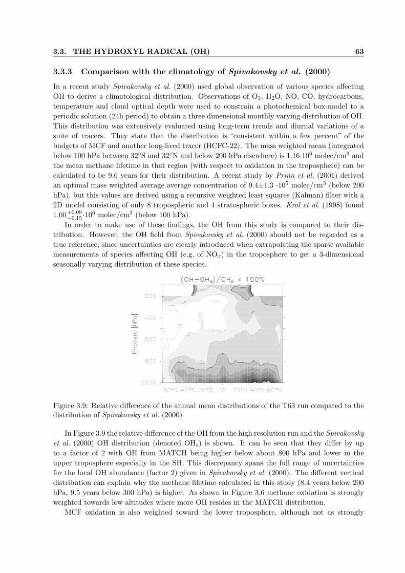
3.3. THE HYDROXYL RADICAL (OH) 63
3.3.3 Comparison with the climatology of Spivakovsky et al. (2000)
In a recent study Spivakovsky et al. (2000) used global observation of various species affectingOH to derive a climatological distribution. Observations of O3, H2O, NO, CO, hydrocarbons,temperature and cloud optical depth were used to constrain a photochemical box-model to aperiodic solution (24h period) to obtain a three dimensional monthly varying distribution of OH.This distribution was extensively evaluated using long-term trends and diurnal variations of asuite of tracers. They state that the distribution is “consistent within a few percent” of thebudgets of MCF and another long-lived tracer (HCFC-22). The mass weighted mean (integratedbelow 100 hPa between 32◦S and 32◦N and below 200 hPa elsewhere) is 1.16·106 molec/cm3 andthe mean methane lifetime in that region (with respect to oxidation in the troposphere) can becalculated to be 9.6 years for their distribution. A recent study by Prinn et al. (2001) derivedan optimal mass weighted average average concentration of 9.4±1.3 ·105 molec/cm3 (below 200hPa), but this values are derived using a recursive weighted least squares (Kalman) filter with a2D model consisting of only 8 tropospheric and 4 stratospheric boxes. Krol et al. (1998) found1.00+0.09
−0.15 ·106 molec/cm3 (below 100 hPa).In order to make use of these findings, the OH from this study is compared to their dis-
tribution. However, the OH field from Spivakovsky et al. (2000) should not be regarded as atrue reference, since uncertainties are clearly introduced when extrapolating the sparse availablemeasurements of species affecting OH (e.g. of NOx) in the troposphere to get a 3-dimensionalseasonally varying distribution of these species.
Figure 3.9: Relative difference of the annual mean distributions of the T63 run compared to thedistribution of Spivakovsky et al. (2000)
In Figure 3.9 the relative difference of the OH from the high resolution run and the Spivakovskyet al. (2000) OH distribution (denoted OHs) is shown. It can be seen that they differ by upto a factor of 2 with OH from MATCH being higher below about 800 hPa and lower in theupper troposphere especially in the SH. This discrepancy spans the full range of uncertaintiesfor the local OH abundance (factor 2) given in Spivakovsky et al. (2000). The different verticaldistribution can explain why the methane lifetime calculated in this study (8.4 years below 200hPa, 9.5 years below 300 hPa) is higher. As shown in Figure 3.6 methane oxidation is stronglyweighted towards low altitudes where more OH resides in the MATCH distribution.
MCF oxidation is also weighted toward the lower troposphere, although not as strongly

64 CHAPTER 3 DESCRIPTION AND EVALUATION OF STANDARD RUN
because the temperature dependence is weaker (kCH4 = 2.45 · 10−12e(−1775/T ) versus kMCF =1.8 ·10−12e(−1550/T ) ). This means that at 220K the rate constant of the CH4+OH reaction dropsto 12% of its value at 298K. For MCF the corresponding fraction is 16%. Additionally, due to thelonger lifetime of methane and relatively more emissions in the SH (about 30% and <1% of thetotal emission of CH4 and MCF are in the SH; Houweling et al. (1999); Midgley and McCulloch(1995)) one would expect a relatively larger fraction of methane to reside in the SH. With thisin mind it is hard to understand why the MCF test suggests too low OH concentrations whilethe methane lifetime is shorter in this study than that of Spivakovsky et al. (2000). This furtherindicates that other factors than the“test quantity” OH are significantly influencing the results ofthe MCF simulation. However, it cannot be ruled out that the lower OH concentrations alreadyabove 800 hPa together with the different temperature dependence is sufficient to explain theresults.
The low southern hemispheric OH in the MATCH simulation is consistent with the overes-timate of CO at these latitudes, although it is unclear whether one is causing the other (andwhich is causing which) or if another factor is involved. The NOx concentrations are certainly animportant factor in determining the OH concentration in the low southern latitudes where NOx
is generally quite low. Some assumptions made by Spivakovsky et al. (2000) to constrain the NOx
distribution in this region can explain part of the difference seen in Figure 3.9. Measurements ofNO during the PEM-Tropics A and TROPOZ II campaigns show lower NO concentrations thanthose used by Spivakovsky et al. (2000).
These authors also used the relative amplitude in the annual cycle of MCF and another tracer(CH2Cl2) at Tasmania to further constrain southern hemispheric OH and conclude from the twotracers that their OH distribution is probably 15-25% or 30-50% (from the two tracer, respec-tively) too high in the SH, but also state that the uncertainty in this estimate from dynamicalparts of the model used to transport these tracer is about ±25%. Overall, this would bring thedistribution of Spivakovsky et al. (2000) in better agreement with the MATCH results.
Finally, it is noted that the OH distribution from the T21 run is up to 40% higher in the trop-ical upper troposphere above about 400 hPa and differences are small in the lower troposphere.Although this may be explained by the stronger convection of CO and hydrocarbons (e.g. iso-prene and its oxidation products) in the high resolution run, the magnitude of the difference issurprisingly large. Above 300 hPa HOx (OH+HO2) is actually larger in the T63 runs, whichconfirms the view that the higher abundance of VOCs in the UT basically shifts the OH/HO2
ratio towards HO2. The calculated OH from the T21 runs is thus in better agreement with thedistribution of Spivakovsky et al. (2000) in the UT.
3.4 NMHCs (Alkanes, Alkenes, Isoprene)
As mentioned in Section 1.2 the oxidation of non-methane hydrocarbons can participate in theproduction of ozone in the presence of sufficient NOx levels. Ethane (C2H6) is also a precursorfor PAN (peroxyacetyl nitrate), which is important for long-range transport of NOx. Propane(C3H8) is a precursor for acetone (CH3COCH3) and PAN. Acetone has gained more interest inthe recent past as it produces HOx in the upper troposphere upon photolysis. Butane (C4H10)is only used here as a pool for all higher alkanes and its distribution will not be evaluated.
Alkenes are very short lived species and their importance is probably only local in thesesimulations, though propene can contribute to PAN formation. Also, changes in local chemistry

3.4. NMHCS (ALKANES, ALKENES, ISOPRENE) 65
(e.g. of HOx) can alter the partitioning of nitrogen reservoir species and thereby have an indirectlong-range effect. Isoprene (a diene) is due to its emission strength of large importance. Especiallyfor isoprene, but also for the other alkenes, however, a direct comparison of model results to pointmeasurements is problematic. Due to their short lifetimes horizontal and temporal gradients canbe quite large and the representativeness of the measurement site for the large grid-box in theglobal model is often not fulfilled. A discussion of some results is nevertheless attempted inSection 3.4.2.
Figure 3.10: Annual mean surface distribution of C2H6 and C3H8 from the T63 simulation.
3.4.1 Ethane and Propane
The annual mean surface distributions of ethane and propane are shown Figure 3.10a and b.The distributions reflect the source distributions, with strong sources from fossil fuel exploitation(e.g. North Siberia, Persian Gulf, North Sea), and the different lifetimes of these compounds.The calculated mean tropospheric lifetime of ethane and propane are about 2.7 months and 28days, respectively. The effects of biomass burning emissions are also visible in Figure 3.10. Thevertical gradient of ethane is therefore similar to that of CO and propane displays a somewhatlarger decrease with altitude.
The comparison of calculated ethane distribution with surface and column measurementscompiled from the literature is presented in Figure 3.11. The simulations and measurements arein quite good agreement for the European stations, although the buildup during winter appears tobe underestimated. However, at most North American stations (e.g. Fraserdale, Harvard Forest)the model significantly underestimates ethane mixing ratios, especially in winter. This indicatesthat the emissions from this region might be underestimated in the EDGAR database, or othersources not accounted for in this study (e.g. biogenic) significantly contribute to the ethane

66 CHAPTER 3 DESCRIPTION AND EVALUATION OF STANDARD RUN
budget at these locations. The free tropospheric stations Izana and Mauna Loa are both alsohigher than simulated mixing ratios, whereas the southern hemispheric stations are fairly wellreproduced. This indicates that the biomass burning source of ethane used here (5.2 Tg(C)/yr)is a reasonable estimate, provided that OH concentrations are not too low (see above). Thisfinding is in agreement with the study of Wang et al. (1998c) which found better agreement witha biomass burning source of 6 Tg(C)/yr than with 2.5 Tg(C)/yr. At Scott Base the seasonalcycle appears to be shifted, with a delay of 1–2 months in the model. A similar deviation wasfound for CO and could thus point toward a problem with the meridional transport between50◦S and 70◦S. Miscalculated abundance and/or seasonal cycle of OH or wrong seasonality inthe sources, however, could also play a role.
Comparison of the simulations with ethane column abundances (last 5 panels in Figure 3.11)shows that the model also tends to underestimate the total column abundance of ethane in thenorthern hemisphere. At Lauder (New Zealand), however, the model is on the high side of themeasurements.
Surface measurements of propane are show in Figure 3.12 along with the model results.The general picture is quite similar to that found for ethane (reasonable agreement in Europe,underestimation in North America). The overestimation of the low resolution run at Birkenes isprobably due to the proximity of the station to the Norwegian oil exploitation field in the northsea, where large emissions of alkanes are predicted by the EDGAR data base (see Figure 3.10).In the SH also an underestimate of a factor of two is visible. Especially interesting is the result atAmsterdam Island. The fact that ethane was well reproduced and propane is underestimated bya factor of two suggests that either the ratio of the emission factors (EF ) of propane and ethane(EFC3H8/EFC2H6) from biomass burning (taken from Andreae and Merlet (2000)) is too lowor that other existing sources with a higher ratio are not included in the model. In particular,oceanic emissions could significantly enhance the background mixing ratios of propane at lowsouthern latitudes. Thus, it is also possible that the oceanic emissions are underestimated in thisregion.
The results from the comparison of these alkanes with airborne measurements gives a similarpicture as for CO. Both compounds are shown in Figure 3.13 (ethane in the upper 3 rows, propanein the lower 3 rows). The vertical profiles of both compounds are mostly well simulated, but somedifferences are also seen. In some regions the observations (ABLE–3A, SONEX–Newfoundland)are underestimated by up to a factor of two (propane over Alaska in summer). The fact that allthree longer lived species (CO, C2H6, C3H8) are similarly underestimated in the Alaska region(ABLE-3A) also suggests that the meteorology of 1998 was not representative for the stateencountered during the measurements.
Unlike for CO the outflow from Asia during PEM-West-B in the“Japan-Coast-E”a significantunderestimate is seen for propane and ethane. In the “Brazil-E” region during the TRACE-Acampaigns the same picture is as for CO is observed: Too low mixing ratios in the upper andagreement in the lower troposphere. Again, the representativeness of these data is questionabledue to sampling in convective outflows. Comparison of with PEM-Tropics A and B campaigns(not shown) which took place during September and March/April over the southern Pacific Ocean(40◦S-0◦) does not reveal a systematic over or underestimation of the model. It is interesting tonote that over the Amazon basin during the ABLE–2A campaign (not shown) propane mixingratios are underestimated by a factor of 3–7 (100–200 pmol/mol observed, versus about 30pmol/mol calculated). The campaign took place at the beginning of the dry season and generally

3.4. NMHCS (ALKANES, ALKENES, ISOPRENE) 67
Figure 3.11: Measured and simulated ethane surface mixing ratios and column abundances (lastrow). Monthly mean measurements are shown as symbols and dotted lines. High and low reso-lution run are solid and dashed lines. Error bars and shaded areas indicate standard deviationsof measurements and model, respectively. Surface data are from Solberg et al. (1996); Lindskogand Moldanova (1994); Bottenheim and Shepherd (1995); Goldstein et al. (1995); Wang et al.(1998c); Greenberg et al. (1996); Touaty et al. (1996); Rudolph et al. (1989); Clarkson et al.(1997) and column data from Notholt et al. (1997); Rinsland et al. (1998, 1999, 2000). At ScottBase individual measurements are marked by crosses. Arrows at Mauna Loa indicate 25th and75th-percentiles. Different years of column measurements over Mauna Loa and Lauder are shownwith different symbols.

68 CHAPTER 3 DESCRIPTION AND EVALUATION OF STANDARD RUN
Figure 3.12: Measured and simulated propane surface mixing ratios. Like Figure 3.11.
sampled air not directly affected by biomass burning (Torres and Buchan (1988), see also NO andPAN measurements presented in Section 3.5 ) so that these high levels of propane are suggestiveof direct biogenic emissions from the rain forest ecosystem.
3.4.2 Ethene (C2H4) and Propene (C3H6)
Alkenes are known to contribute to ozone production in polluted environments. Only a simplerepresentation of the two smallest alkenes, ethene (or ethylene) and propene (or propylene),has been included to account for this local effect. The distributions of these two compoundsare shown in Figure 3.10 c and d. The calculated mean lifetimes are 2.2 days and 16 hours,respectively. Thus, the distribution mainly reflects the assumed source distributions. It can beseen that biogenic sources (e.g. in Amazonia or South-East U.S.) and biomass burning (Brazil,Africa) are strong contributors to the abundance of these alkenes. At low southern latitudesoceanic influence is also visible, which is in part due to the low OH abundances, but is mainlybecause the ocean emissions used in this study (Bates et al. (1995)) are largest at these latitudes.
A comparison with surface measurements for ethene and propene is presented in Figure 3.14.A seasonal cycle driven by OH with lowest values in summer is seen at most stations. Theseasonal cycle in the biogenic emission cannot compensate for the decreased lifetime in summer.As mentioned before comparison of station measurements with short-lived substances is notstraightforward. Considering the high degree of variablity, model and observations are judgedto be consistent with only a few exceptions. At the remote arctic and free tropospheric stationsZeppelin (near Ny Alesund) and Izana both compounds are strongly underestimated. For theZeppelin measurement, Solberg et al. (1996) argued that local biogenic source are the most likelycause for the relatively high values at such a remote site. At some Canadian stations a secondarylate summer maximum of ethene can be seen in the model, but not in the observations. This islikely due to the assumed biogenic ethene emissions of 10 Tg/yr. The estimate is highly uncertain

3.4. NMHCS (ALKANES, ALKENES, ISOPRENE) 69
Figure 3.13: Airborne observations of ethane (first three rows) and propane (last three rows) inunits of pmol/mol compared to model simulations, as in Figure 3.5.

70 CHAPTER 3 DESCRIPTION AND EVALUATION OF STANDARD RUN
especially considering the stress induced emissions, and it appears to be too large for the northernAmerican region. On the other hand, the model is consistent with the few measurements made inSouth America at strongly biogenically-influenced sites. In the Amazon basin the model predictsabout 1.3 nmol/mol of ethene and 0.2 nmol/mol of propene, in agreement with the observations(Greenberg and Zimmerman (1984); Zimmerman et al. (1988)). Compared to measurementsin Venezuela (Donoso et al. (1996)) C2H4 is slightly overestimated at some stations or seasons(e.g. Buja: 0.9 nmol/mol simulated versus 0.6±0.3 observed), but too low at others (e.g. Calabozoin September: 0.8 versus 1.5 nmol/mol). Simulated propene appears to be mostly lower than theobservations. However, due to problematic representativeness of these stations and too coarsemodel resolution no firm conclusions can be made at this point.
There are also measurements of alkenes from ship cruises (e.g. Bonsang and Boissard (1999)and references therein), but Donahue and Prinn (1993) suspect that many observation usingcanister samples, which yielded significantly higher values than in situ measurement techniques,suffer from systematic problems. Even only comparing to in situ observation (e.g. Donahueand Prinn (1993), during the SAGA 3 campaign) shows that the model is usually lower thanobservations by more than a factor of 2. The typical ranges found by Donahue and Prinn(1993) over the Pacific near the equator for ethene and propene were 30–100 pmol/mol and 20–80 pmol/mol, respectively, whereas the model shows only 10–20 pmol/mol and 2-6 pmol/mol.Thus, even the 90% upper limit of the emission estimate of Plass-Dulmer et al. (1995) appliedin MATCH appears to be too low, or the latitudinal distribution assumed in this study is toomuch weighted toward the southern low latitudes.
Airborne measurements have also been made during several campaigns. The problem ofrepresentativeness is even more severe for these measurement. Therefore only the general pictureobtained by the comparison is discussed here.
The ethene observations during ABLE-3B over Canada, PEM-West A+B and TRACE-A arereasonably well reproduced (not shown). This is especially interesting for the biomass burningregions in Brazil and South Africa and supports the emission ratios used for the alkenes, whichwere taken from Andreae and Merlet (2000). The vertical profile is more sensitive to the differentvertical transport characteristics of the two resolutions and upper tropospheric concentrations ofethene over the biomass burning regions are overestimated by the high resolution run, whereasthe low resolution run is in agreement with the observations.
Measured mixing ratios of propene in the free troposphere are very low (<10 pmol/mol,probably close to the detection limit). The model produces a pronounced C-shaped profile oversource regions whereas the measurement appear to be more uniform. This could indicate tooweak mixing in the updraft calculated by the convection scheme. When larger amounts are seenin the measurements the magnitude is correctly simulated by the model.
3.4.3 Isoprene
The important role of isoprene in atmospheric chemistry was already introduced in Section1.2. Its source strength exceeds those of any other biogenically emitted compound known sofar. The most important sink of isoprene is reaction with OH (85%), but reactions with ozone(11%) and NO3 (4%) are also non-negligible. It is also noted, that biologically mediated loss ofisoprene to different types of soil was also observed (Cleveland and Yavitt (1997)), but a firstextrapolation to the global scale resulted in only about 20 Tg/yr compared to 300-500 Tg/yrof direct emissions. Recently, Sanhueza et al. (2001) could infer from surface measurements

3.4. NMHCS (ALKANES, ALKENES, ISOPRENE) 71
Figure 3.14: Measured and simulated ethene (C2H4, first three rows) and propene (C3H6, lastthree rows) Symbols and lines like in Figure 3.11. Additionally to means (square), also medianvalue (star) is shown for some stations.

72 CHAPTER 3 DESCRIPTION AND EVALUATION OF STANDARD RUN
made at a savanna site in Venezuela and box model calculations that deposition of isoprene andits oxidation products methyl-vinyl-ketone and/or methacrolein, not accounted for in presentmodels, must be a significant loss process for these compounds at this site.
The monthly (24h-averaged) surface distribution of isoprene is shown in Figure 3.15 forJanuary and July. Due to its short lifetime of a few hours the distribution closely follows theemissions shown in Figure 2.4. Maximum values of 13 nmol/mol are shown in the central Amazonbasin. Even higher maximum values of up to 27 nmol/mol are found in both runs for othermonths. It is noted that these results are obtained with a reduced source strength of isopreneof 350 Tg(C)/yr compared to Guenther et al. (1995) (500 Tg(C)/yr) and the procedure to emitisoprene with an even mixing ratio over the PBL height.
Even more so than for the other alkenes, comparison of measurements of isoprene at singlelocations is problematic due to the coarse model grid and small scale horizontal variations inits concentration. Nevertheless, the ensemble of model/measurement comparisons can give in-dications on general tendencies of the model to over or under-predict concentrations in certainecosystems. A compilation of available surface measurements along with model predictions islisted in Table 3.5. It is noted that the model values are 24h averages, whereas the measure-ments are usually made during daytime. From box-model simulation one can estimate that the24-average value is about 50-75% of mid-day concentrations.
Figure 3.15: Mean (24h-averaged) isoprene surface mixing ratios for January and July. Whitespots over Amazonia are values above 10 nmol/mol.
The model appears to be in basic agreement with measurements made in North America.Measurements in Japan are expected to be higher, since the model grid-cells actually also containan oceanic fraction. The values in the Georgian Republic are obtained in a coniferous forest onthe southern slopes of the Caucasus Mountains, which might not be representative of the largerarea. The model significantly overestimates mixing ratios found in the central Amazon region,sometimes by a factor of 3 or more. The Amazonia sites are probably quite representativeof the region, since no major inhomogeneities in the vegetation are expected. The situationis different for the Peru site. It is located in a region where a strong horizontal gradient inisoprene is calculated by the model with mixing ratios below 1 nmol/mol to the west to morethan 10 nmol/mol east of the site (within 2-3 grid cells even at the higher resolution). If themodel value is obtained from interpolation of adjacent grids to the exact position of the site a

3.4. NMHCS (ALKANES, ALKENES, ISOPRENE) 73
Tab
le3.
5:C
ompa
riso
nof
obse
rved
isop
rene
mix
ing
rati
os(i
nnm
ol/m
ol)
wit
hm
odel
calc
ulat
ions
.24
-hou
rm
eans
are
mar
ked
wit
h“2
4h”,
othe
rwis
eda
ytim
eva
lues
are
repo
rted
.M
odel
valu
esar
em
onth
ly(2
4ho
ur)
aver
ages
.In
brac
kets
max
imum
and
min
imum
ofsi
ngle
mea
sure
men
ts.
Loc
atio
nT
ime
Lat
.L
on.
Obs
erva
tion
sT
63T
21R
efer
ence
Can
ada,
Egb
ert
July
44-7
90.
50.
30.
4B
otte
nhei
man
dSh
ep-
herd
(199
5),
Kej
imku
jikJu
ly45
-65
2.0
0.2
0.3
Bot
tenh
eim
and
Shep
-he
rd(1
995)
,Fr
aser
dale
Jul.-
Aug
.50
-82
0.5-
50.
50.
4Jo
bson
etal
.(1
994)
Niw
otR
idge
Aug
.-Se
pt.
40-1
050.
6(0
.2-1
.8)
0.2
0.1
Gre
enbe
rgan
dZ
imm
er-
man
(198
4)N
ov.
40-1
050.
1(0.
03-0
.2)
0.04
0.04
Gre
enbe
rgan
dZ
imm
er-
man
(198
4)G
eorg
ian
Rep
.Su
mm
er42
431.
4(m
ax.
6)0.
20.
2Sh
awet
al.
(198
3)Ja
pan
July
,24
h38
140
0.3
0.2
0.1
Yok
ouch
i(1
994)
Nov
,24h
3814
00.
20.
020.
01Y
okou
chi
(199
4)A
laba
ma
Jun.
-Jul
.,24
h32
-88
3.8
(1-7
)2.
92.
4M
ontz
kaet
al.
(199
3)A
maz
onia
Jul.
2-6
02.
2(1
.2-3
.2)
6.7
11.0
Ras
mus
sen
and
Kha
lil(1
988)
Am
azon
iaye
ar-r
ound
2-6
02.
4(1
.0-5
.2)
6.1
9.0
Gre
enbe
rgan
dZ
imm
er-
man
(198
4)A
maz
onia
Jul.-
Aug
.-2
-60
2(1
.1-2
.7)
6.4
14.5
Zim
mer
man
etal
.(1
988)
Per
uJu
ly-5
-77
3.3
10.3
15.6
Hel
mig
etal
.(1
998a
)V
enez
uela
,Buj
aSe
pt.
9-6
23.
33.
83.
0D
onos
oet
al.
(199
6),
Auy
ante
puy
Apr
.,24
h6
-62
1.6
1.9
3.1
Don
oso
etal
.(1
996)
,C
alab
ozo
Sep.
-Oct
.,24h
9-6
70.
8(0
.2-3
.1)
5.9
7.8
Sanh
ueza
etal
.(2
001)
,C
alab
ozo
Mar
.-A
pr.,2
4h9
-67
0.5
(0.1
-1)
0.5
0.5
Sanh
ueza
etal
.(2
001)
,P
arup
aJa
n.-F
eb.
6-6
20.
5(0
.1-1
.2)
1.2
2.3
Sanh
ueza
etal
.(2
001)
Suri
nam
(PB
L)
Mar
.2-
7-5
4-58
3.5
(0.5
-7)
2.8
2.5
War
neke
etal
.(2
001)

74 CHAPTER 3 DESCRIPTION AND EVALUATION OF STANDARD RUN
smaller value (5.7 and 5.2 nmol/mol for T63 and T21 run, respectively) is found than given inTable 3.5. Since the measurement site is well within the primary rain forest the value of thenext grid cell to the east is used here instead. Both methods yield a significant overestimationcompared to the daytime values of Helmig et al. (1998a).
Vertical profiles of isoprene have been reported by Helmig et al. (1998a); Andronache et al.(1994), and Warneke et al. (2001). The modeled steep gradient with values of less than 5% of thesurface mixing ratio at 1.5 km altitude are consistent with the first two studies. Over Surinam(LBA-Claire campaign), however, the decrease in the model is much too fast and only about 100pmol/mol are left at about 2.5 km, whereas the observations are still above 1 nmol/mol up to4 km (Warneke et al. (2001) during the LBA-CLAIRE6 campaign). These measurements, madewith the PTR-MS7 technique, however, only give information on the mass of the molecules. Themass signals then have to be attributed to molecules that can be expected under those condition(see e.g. Williams et al. (2001)). Although the full signal at mass 69 was assumed to be isoprene,other minor contributors may be possible. Therefore, an uncertainty of 0.5 nmol/mol has beenassigned to these measurements (Warneke et al. (2001)). Even with this uncertainty, it appearsthat the shallow convection reaching up to about 4 km altitude often encountered during thecampaign is not reproduced by the model, which can be seen in the stronger than observeddecrease with height (not shown).
Mixing ratios of isoprene sometimes well above 1 nmol/mol have been observed during theLBA-Claire campaign at about 11 km altitude, provided no other substance is contributingsignificantly to mass 69. The model only reaches maximum mixing ratios of up to 120 pmol/molover Surinam (at T63), but can reach nmol/mol levels over the central amazon basin. Notethat the T21 run produces much smaller isoprene mixing ratios in the upper troposphere (about100-300 pmol/mol over the same region) due to the difference in convective pumping betweenthe two runs.
Despite the problems mentioned with the comparison of such a short lived compounds, weconclude that calculated isoprene mixing ratios are too high over the rain forest regions of SouthAmerica. More vigorous vertical mixing in the boundary layer could help to reduce the discrep-ancy but it would probably also produce even higher concentrations in the upper troposphere,which appear to be unrealistic, at least for the high resolution run. Especially considering thatJacob and Wofsy (1990) assumed an uptake of isoprene through the leaf stomata, but no exper-imental confirmation of this is available.
The overestimated isoprene concentrations over the Amazon region has also been found inother studies (Houweling et al. (1998); Granier et al. (2000)) and appears to be an unsolvedproblem in current research of biosphere-atmosphere interactions. The uncertainties regardingthis compound are still very large and more observations are clearly needed to resolve the problem.
6Cooperative LBA Airborne Regional Experiment (LBA: Large-scale Biosphere-Atmosphere experiment).7Proton-Transfer-Reaction Mass Spectrometer

3.5. NITROGEN-SPECIES 75
3.5 Nitrogen-Species
Nitrogen oxides (NOx=NO+NO2) play a central role in atmospheric chemistry (see Chapter1) in controlling destruction and production of ozone and influencing OH. Their abundance inthe atmosphere is also linked to a number of temporary reservoir species (e.g. PAN, HNO3
or other organic nitrates). Accurate understanding and simulation of the distribution of thesereactive nitrogen species (NOy = NOx + NO3 + 2·N2O5 + HNO4 + PAN + other organicnitrates) is therefore a key to understanding present and future impacts of human activities onthe atmosphere. This is also underlined by the fact that responses of ozone production to changesin NOx are highly non-linear (e.g. Liu et al. (1987); Lin et al. (1988)).
The basic chemistry of nitrogen compounds was reviewed in Sections 1.1 and 1.2. In orderto get a better overview on the dominant processes, some budgets and the distribution of themost important compounds are presented next, before an extensive comparison to observationsis shown in the subsequent subsections.
3.5.1 The Distribution and Budget of Nitrogen Species
Table 3.6 shows the annual mean tropospheric burden of all nitrogen containing compounds in-cluded in the chemical mechanism. Results from a sensitivity simulation with an increased rate ofthe dissociation reaction of PAN are also included and will be discussed further in Section 3.5.4.Clearly, in all simulations PAN is the largest reservoir species for NOy, followed by NOX (theextended NOx-family: NOX = NOx + NO3 + 2·N2O5 + HNO4) and HNO3. In the NOX-familyNO2 is the largest contributor (62%), followed by NO (18%) and HNO4 (17%). ONIT, the or-ganic nitrate pool from higher alkanes is also a significant reservoir. The large difference betweenthe T63 and T21 in MPAN, a PAN–analog from the oxidation of isoprene, is due to strongerconvection in the T63 run (see below). The other nitrates from isoprene oxidation are only smallcontributors to the mean tropospheric NOy budget, owing to their short photochemical lifetimes(21 and 10 hours for ISON and NACA8, respectively). For the smaller nitrate NACA (nitrooxy-acetaldehyde), which is formed from ISON upon reaction with OH, the reactivity and photolysisrates are assumed to be the same as for acetaldehyde (CH3CHO). With this assumption, whichalso implies a low solubility9, only 2% of the NACA produced is lost through dry deposition,with the rest releasing back NO2. Omission of this nitrate would therefore only mildly affectthe results, and, considering uncertainty in the chemistry, the loss or fixation of nitrogen by thiscompound is probably sufficiently represented by ISON alone.
Table 3.6: Tropospheric burden of nitrogen-containing compounds in MATCH (in Gg(N) =109g). “T21-LOWPAN” denotes a run with PAN dissociation reaction increased to the upperlimit of the range of uncertainty (see text).
Species Run PAN NOX HNO3 ONIT MPAN ISON NACA NOy
Burden T63 257 154 95 33 23 7 3 572in [Gg(N)] T21 204 125 81 32 9 6 3 460
T21-LOWPAN 144 122 80 33 6 6 3 394
8See Table 2.1 for the list of species.9Assumed equal to that of acetaldehyde.

76 CHAPTER 3 DESCRIPTION AND EVALUATION OF STANDARD RUN
Table 3.7: Global annual mean tropospheric budget of NOy and HNO3. All terms are inTg(N)/yr.
NOy T63 T21 HNO3 T63 T21Emissions NO 43 43 Sources Transport 0.3 0.4Wet Deposition HNO3 21.4 23.4 NO2+OH+M 21.8 18.9
ISON 0.9 1.5 N2O5 heterogeneous 13.2 16.7total 22.3 24.9 N2O5+H2O (homogen.) 3.7 1.7
Dry Deposition HNO3 16.0 13.1 CH3CHO+NO3 0.25 0.20NOX 3.1 3.7 HCHO+NO3 0.33 0.24PAN 0.6 0.8 Sinks Dry Deposition 16.0 13.1ISON 0.8 0.6 Wet Dep. - Large Scale 19.2 19.3MPAN 0.2 0.3 Wet Dep. - Convective 2.2 4.0total 20.7 18.6 HNO3+OH 1.4 1.3
Lifetime (days) NOy 4.9 d 3.9 d HNO3+hν 1.0 1.0
The lower resolution run predicts less PAN, which is understandable since less convection willlead to less PAN in the UT, where its lifetime is longest. The lower NOx abundance in the T21runs is in part also an effect of the corrected wet skin fraction in the T21 simulation, which leadsto more efficient dry deposition of NO2 over the affected regions. A run with the same wet skinfractions as the T63 simulation results in 144 Gg(N) of NOX; the other totals are only slightlyaffected. The mean tropospheric lifetime of NOy is higher in the high-resolutions run (about 5days) than in the lower resolution run, reflecting the tendency in the T63 simulation to storemore nitrogen in the long lived PAN.
In order to examine possible reasons for an overestimation of PAN found in comparison withobservations (see below) a sensitivity simulation has been performed (“LOWPAN”), in which atwo times faster decomposition rate10 of PAN is used in accordance with the range of uncertaintygiven in DeMore et al. (1997) and Tyndall et al. (2001). Although the resulting burden of PANis reduced by about 30% compared to the corresponding standard simulation it is still the mostabundant nitrogen-species in the troposphere. NOX and HNO3 are only slightly affected.
The loss pathways for NOy from the atmosphere are listed in Table 3.7. Here, HNO3 playsthe key role, with a calculated 85% of the total loss occurring via deposition of this compound.This number, however, also includes a fraction of loss occurring through deposition of aerosols.For the hydrolysis reaction of N2O5 on sulfate aerosols it was assumed that the HNO3 is releasedback to the gas phase. In reality also a fraction of the aerosols could deposit directly beforere-releasing HNO3. Also, it has been argued in Section 2.3.5 that the estimate of wet depositionof highly soluble species such as HNO3 is likely on the high side, so that the fraction given abovecan be regarded as an upper limit.
Due to its importance in removing reactive nitrogen from the atmosphere a more detailedbudget of nitric acid is also shown in Table 3.7. Gas phase production via reaction of NO2 withOH and the heterogeneous pathway are dominating the production terms. However, homoge-neous production (recently found to occur by Wahner et al. (1998)) is also a non-negligible term,being larger than each of the two photochemical loss terms (via OH and photolysis). These termsmay also be compared with the much faster exchange rates within the NOx-family (NO→NO2,
10For reaction R87 in Table A.1 k87 = k79 / 4.5·10−29exp(-14000/T) was used.

3.5. NITROGEN-SPECIES 77
NO2→NO) which are globally averaged (in the troposphere) about 5000 Tg(N)/yr in both direc-tions. The budget of HNO3 also implies that the annual global mean lifetime of nitric acid againstphotochemical oxidation is about 14 days, whereas its lifetime against dry and wet depositionis only about 2.5 days. In the tropics the lifetime of HNO3 against rainout can even be belowone day (see e.g. Brasseur et al. (1998)). It is interesting to note that globally averaged largescale precipitation is the dominating pathway of nitric acid wet deposition (90%). In the tropics(20◦S–20◦N) convective core precipitation11 has a larger contribution to total wet scavenging(18%).
The production and loss terms of PAN (not listed) are dominated by the fast equilibriumbetween the PA-radical (peroxy-acetyl radical, CH3CO3) and PAN (about 150 Tg-N/yr in eachdirection). Photolysis and reaction with OH have only 1% and 0.1% of this turnover. However,in the upper troposphere above 340 hPa (σ < 0.341) photolysis is the dominant pathway (93%)and reaction with OH (5%) and thermal decomposition (2%) account for the rest.
It is also interesting to determine the fraction of NOy which is exported out of the mainsource region. For the T21 run it is calculated that only about 19% of the emissions into thecontinental PBL (σ > 0.778, continents defined by the model’s land/sea mask) are exported outof this region and the rest is lost from the atmosphere via the pathways described above. Notethat the net export is put in relation to the emission strength, which means that some importis not accounted for in the estimate. The fraction is not very different when calculated for thecontinental troposphere (16%) or the continental boundary layer of the U.S. (17%). The lattervalue is in good agreement with a corresponding total of 16.2% obtained by Horowitz et al. (1998)in a regional modeling study.
The distribution of NOx for two months is shown in Figure 3.16. The largest concentrationsare simulated during winter in the industrialized regions of the NH. The impact of biomassburning is also visible in both months in Africa. Enhanced mixing ratios in the north Atlanticand Pacific are due to ship emissions. In other regions of the oceans mixing ratios of NOx are verylow (few tens of pmol/mol or lower). While the zonal mean mixing ratio of PAN usually increaseswith height, NOx concentrations mostly show a “C”-shaped profile. This can be explained bysurface emissions that are efficiently converted into PAN and also to other nitrogen-reservoirs(e.g. HNO3, HNO4, ONIT) moving to higher altitudes and by stratospheric influx, and lightningNOx and a longer lifetime of NOx in the upper troposphere. Especially during winter (NH) inthe middle and upper troposphere nearly all reactive nitrogen is in the reservoirs as opposed tosummer when higher NOx concentrations are seen. Lightning, which more intense during thesummer season also helps maintaining this seasonal cycle.
The zonal mean distribution of PAN depicted in Figure 3.17 mainly reflects its increasinglifetime with altitude and the distribution of its precursors. The low resolution run differssignificantly from that distribution. Surface PAN mixing ratios are higher in the regions where themaxima are seen in Figure 3.17, but less PAN is found in the UT: about 270 pmol/mol in the zonalmean compared to about 400 pmol/mol in the T63 run in July. The effects from smoothing ofthe non-linear chemistry in the T21 run should actually lead to higher PAN production, since theprecursors (NOx and hydrocarbons) are more efficiently mixed. The higher PAN concentrationsin the UT at T63 resolution are therefore most likely due to more efficient vertical transport. Inturn this indicates that a realistic representation of vertical transport is an important factor incalculating upper tropospheric PAN concentrations.
11Note that precipitation from convective anvils is actually counted as “large scale” precipitation.

78 CHAPTER 3 DESCRIPTION AND EVALUATION OF STANDARD RUN
Figure 3.16: The simulated surface (left) and zonal mean (right) distribution of NOx (from theT63 run) for January and July.
Figure 3.17: The simulated surface (left) and zonal mean (right) distribution of PAN (from theT63 run) for January and July.

3.5. NITROGEN-SPECIES 79
Figure 3.18: The annual zonal mean distribution of other nitrogen containing compounds.Isoprene-N denotes the sum of the compounds ISON, MPAN and NACA.
For the other nitrogen containing compounds only the annual zonal mean is shown in Figure3.18. The distribution of HNO3 displays a minimum in the upper tropical troposphere of only5 pmol/mol. As will be shown in Section 3.5.5 these extremely low concentrations are mainlycaused by the scavenging of nitric acid on ice particles in combination with gravitational settlingor rainout. Pernitric acid (HNO4) is transported with the NOX-family and not assumed to bewashed out by precipitation. It is thermally quite unstable in the lower troposphere, and thereforeappreciable amounts are only calculated in the UT. The alkyl-nitrates, represented by the speciesONIT, are mainly formed from the higher-alkanes surrogate C4H10 in the chemical mechanism.ONIT is therefore only found in larger amounts in the northern hemisphere industrialized regions,where these species are mainly emitted. Nitrates from isoprene (ISON, MPAN and NACA) aremost abundant where isoprene emissions coincide with sufficient NOx. Through convection inthe tropics more than 50 pmol/mol of these compounds are calculate in the high resolution run.In the T21 run the isoprene-related nitrates only reach about 15 pmol/mol in the zonal meanin the UT, but higher mixing ratios (50 pmol/mol) near the surface. This is another clear signfor the weaker convection in that run and shows the strong implications this can have on thevertical distributions of some species.
3.5.2 Comparison of NO2 with GOME-Satellite Column Retrievals
Satellite observations of tropospheric constituents are much more difficult than for the strato-sphere due to interferences with clouds and aerosols, inhomogeneities in the ground albedo andthe stratospheric contributions. While the retrieval of height resolving information on the tropo-spheric composition will only be available in the near future (see e.g. Singh and Jacob (2000)),column integrated abundances of a few species (O3 NO2, HCHO, SO2, BrO) have been retrieved

80 CHAPTER 3 DESCRIPTION AND EVALUATION OF STANDARD RUN
from the Global Ozone Monitoring Experiment (GOME), and retrieval algorithms are continuingto be improved. A first broad comparison of NO2 column data provided by A. Richter (Richterand Burrows (2001)) with MATCH results is presented in this section. The comparison in thisstudy is merely aimed at getting an overview on strong and weak points of the NOx emissionsdistributions and their seasonality applied in this study.
The GOME Retrieval and Error Estimate
GOME is installed on the ERS-2 satellite, which is in a sun-synchronous polar orbit that crossesthe equator at 10:30 local time. Measurements in middle and low latitudes are therefore alwaystaken in the late morning. Details on the retrieval can be found in Richter (1997) and Richterand Burrows (2001), and the procedure is only briefly sketched here.
The slant column retrieval uses the Differential Optical Absorption Spectroscopy (DOAS)technique in the wavelength interval 425-450 nm. The stratospheric NO2 content is removedsimply by subtracting the NO2 slant column calculated for the 180-190◦ longitude sector, which isassumed to be essentially free of tropospheric NO2. Another assumption implied by this approachis a zonally symmetric distribution of NO2 in the stratosphere, which can be problematic nearthe edges of the polar vortex, especially over the northern high latitudes in winter and spring.
The slant columns then need to be converted to vertical column abundances. The two quan-tities are linked through the so called air-mass factor (AMF). Its calculation involves severalparameters (solar zenith angel, cloud cover, vertical NO2 profile, aerosol loading and propertiesand the surface albedo) and further assumptions have to be made in order to constrain them.Richter and Burrows (2001) used clear sky conditions, maritime aerosol, a constant surface albedoof 0.05 and a constant mixing ratio of NO2 within the lowest 1.5 km (zero NO2 above) to calcu-late the AMF. If substantial amounts of NO2 are present in the upper troposphere, the retrievalalgorithm would overestimate its contributions (A. Richter, private communication, 2001). Onlypixels with a cloud cover below 0.1 are used in the data merges provided on a 0.5◦×0.5◦ grid.The error from the slant columns calculation is about 1·1015 molecules/cm2. The error in thecalculation of the air-mass factor calculation is estimated to be up to a factor of 2 for clear skyconditions and most NO2 residing in the lowermost troposphere (Richter and Burrows (2001)),but can easily exceed a factor of 2 when large amounts are present in the upper troposphere (A.Richter, personal communication, 2001).
Examples of the GOME NO2 data are shown in Figure 3.19 for two months. Enhancedcolumn abundances over industrialized regions and typical biomass burning regions are clearlyvisible. The high values over high latitudes in Siberia in January are probably affected bysnow cover, which drastically changes the surface albedo and makes the assumptions for theAMF calculations invalid. Enhanced values south of 40◦S in September are probably due toan asymmetry in the polar vortex. The monthly mean data from the period January 1996 –August 2000 are averaged per month in the following comparison in an attempt to smooth theeffect of inter-annual variability in biomass burning. Using only the year 1998 (correspondingto the meteorological input data used for the model) was also tested, but the main conclusionsremained the same.
MATCH data are only available as monthly means (i.e. day-and-night averages), which meansthat a “sampling error” needs to be considered when comparing this to the late morning NO2
values seen by GOME. The factor to correct for this effect, hereafter referred to as the “samplingcorrection factor” (SCF), depends on several parameters:

3.5. NITROGEN-SPECIES 81
1. Length of the day: The shorter the day, the higher the SCF, since all NOx is in the formof NO2 during night.
2. Ozone concentration: The more ozone, the lower the SCF. The reaction of O3 with NO isthe dominant pathway for conversion of NO to NO2 and thus affects the NO/NO2 ratioduring the day.
3. Solar insulation: The more UV radiation, the higher the SCF. Photolysis of NO2 is the mostimportant process for the conversion of NO2 to NO and thus also influences the NO/NO2
ratio. This parameter is also dependent on surface albedo, cloudiness and the solar zenithangle.
4. Vertical distribution of NOx: The more NOx resides in the upper troposphere, the higherthe SCF. This is because the NO2/NOx ratio during day decreases with altitude due tothe higher photolysis rate of NO2 and the negative temperature dependence of the NO+O3
reaction. This results in a lower column integrated value found for NO2 at 10:30, if largeamounts of NOx are in the upper troposphere (e.g. from lightning).
The combined effects of these parameters is not easy to judge; thus, a globally constant SCFis used here. Through test simulations with MATCH over a few days in January, July, andSeptember with output every hour it was calculated that the SCF can range from 0.4 to 1 forregions with a tropospheric NO2 column abundance greater than 1·1015 molec./cm2. In mostcases values where about 0.6-0.8. A constant SCF of 0.7 is used in the following comparison,but an uncertainty of about 20-30% cannot be avoided by this procedure. A further problemwith determining the SCF is that it is not likely representative for the “clear sky” selection in theGOME data, because under these conditions a smaller NO2/NOx ratio would be expected dueto a higher photolysis rate of NO2. A globally averaged “clear sky SCF” is therefore likely lowerthan the value 0.7 applied here.
Comparison by Region
In Figure 3.20 the ratio of GOME-NO2 and the model results are plotted for 6 months. Thetropospheric column is separated in the model using the same “clean sector” technique as for theGOME data and a correction factor of 0.7 is applied globally. In view of the systematic errorin the GOME data only areas are plotted where either GOME or MATCH tropospheric NO2
columns reached values higher than 1·1015 molec./cm2. The green colors mark regions where theagreement is within a factor of 2 and thus model and GOME NO2 are considered to be consistent(see error estimate above). Additionally, the seasonal cycle is depicted at selected coordinates inFigure 3.21 in order to facilitate the discussion. The focus of this discussion is on regions wherediscrepancies between model and satellite data are seen, and it is attempted to identify the mostlikely source category of NOx by inspection of the emission fields.
It is also noted that the results are very similar for the low resolution run, but some resultsseen in the comparison with the high resolution run are not found in the T21 runs because theyare too small to be resolved on the coarser grid.
Europe While in central Europe the model is only slightly higher than the GOME values,especially in winter, a significant overestimation can be seen over parts of north-eastern Europe.

82 CHAPTER 3 DESCRIPTION AND EVALUATION OF STANDARD RUN
Figure 3.19: GOME tropospheric NO2 column abundances (in 1015molecules/cm2). Averages ofmonthly means from the period January 1996 to August 2000 are shown (January 1998 missing).
Figure 3.20: Ratio of tropospheric column NO2 (MATCH/GOME) for January , March, May,July, September, and November. GOME data are means of monthly means from 1996-2000(January 1998 missing). Only regions are plotted where either GOME or MATCH values areabove 1·1015 molec./cm2.

3.5. NITROGEN-SPECIES 83
The emission data for industrial NOx, taken from the EDGAR database are for the year 1990.It seems that the strong decrease in industrial activities in the former “Eastern Bloc” countriesduring the 90s are therefore not included in the dataset and lead to this overestimation. Theseasonal cycle of NOx, which in the model is mainly determined by the NO/NO2 partitioning andthe lifetime of NOx (the industrial emission strength is constant over the year), is very similarto that seen by GOME (1st panel in Figure 3.21).
An interesting point is the strong overestimation (factor 3-10) of MATCH in January overthe northern Atlantic west of France. Since westerly winds are dominating in the region, thismust be attributed to a local source. Furthermore, a corridor of column NO2 of more than0.5·1015 molec/cm2 is calculated in January over the North Atlantic (at about 45◦N-53◦N, notshown), whereas GOME only sees background noise (Figure 3.19). The two possible sources areaircraft and ship emissions. Inspecting the source distributions of these sources12 reveals thatthe band of enhanced NO2 columns in the model is clearly caused by aircraft emissions in theNorth Atlantic flight corridor. Effects of aircraft NOx emissions in other regions or season are notpredicted by the model, probably because this is the region over ocean with the highest emissionrate and during winter the lifetime of NOx is longest. Over continents the effect is masked byother sources. The overestimation east of the Bay of Biscay cannot be unequivocally attributedto one source type, but at least in the southern-most part ship emissions are more likely. Lackingevidence for the effects of ship-NOx was also suggested by a comparison of marine boundary layermeasurements with similar model results (Kasibhatla et al. (2000)) and early plume processes notaccounted for in large scale models were suspected as a possible explanation. Similar findingswere made by Meijer et al. (1997), who studied the effect of nitrogen conversion in aircraftexhaust plumes. They came to the conclusion that the perturbation in NOx can decrease by15-55% when taking into account plume-processing. The disagreement found here lends supportof the hypothesis that plume chemistry of nitrogen compounds can be important for aircraft andship emissions. These results further underline that more research is needed on sub-grid chemicalphenomena.
North and Middle America Like for the most polluted European regions, the seasonalcycle (2nd panel in Figure 3.21) is qualitatively reproduced, but the values obtained by MATCHare on the high side, especially in winter. In the mid-west of the U.S. concentrations are signifi-cantly overestimated by the model (about a factor 3).
The overestimated NO2 columns over Middle America in March (and April, which is notshown) can be clearly attributed to the biomass burning data set, which predicts burning forthese months and is the dominant source during this time of the year. Thus, either the totalbiomass burned is overestimated or the burning season is too short in the Galanter et al. (2000)emission data.
Asia Several discrepancies can be seen over eastern Asia. Where strong industrial emis-sions are found in the GOME data (mainly over north-eastern China), the model results areconsiderably lower, especially in winter. The bulge in the model calculation in summer corre-lates well with biomass burning assumed to occur during that time, but it does not show upin the satellite data. This suggests that the burning activity is too high in the Galanter et al.(2000) data set, which could also in part be responsible for the overestimated CO seen at the
12For the aircraft emissions see Lawrence et al. (1999b).

84 CHAPTER 3 DESCRIPTION AND EVALUATION OF STANDARD RUN
Figure 3.21: Seasonal variation of GOME tropospheric NO2 column data (solid line) and modelsimulation (T63: dashed, T21: dotted line) for selected regions. The GOME values are obtainedby averaging over the respective T63 grid cell.
Tae-ahn Peninsula station (Section 3.1, Figure 3.3). On the other hand, in south-eastern Chinathe model overestimates and it appears from a comparison of the distribution of the NO2-columnsthat emissions are too evenly distributed over east China in the EDGAR data (see Figure 2.2a).Further question which need to be addressed in this
Africa and South America In Africa the seasonality and magnitude of the NO2 columnsare in good agreement with the satellite data for most regions. This is a significant improvementover the previously used data set of Hao and Liu (1994). In the results from MATCH-2.0(Lawrence et al. (1999b)), which applied the datasets from Hao and Liu (1994) much too sharpand too strong maximum columns are found in southern and south-western Africa, the Sahel andalso in south-eastern Brazil (not shown). The seasonality of the Hao and Liu (1994) data is alsonot consistent with GOME data, being to late in SW Africa and too early in SE Brazil by about1 month, respectively. However, some discrepancies are also seen with the emission data fromGalanter et al. (2000). The burning in the Sahel region during November to February appearsto be too high and the underestimate in May in SW Africa (at about 15◦S) suggests that theburning season may already start in this month. Lightning, as an alternative explanation, is notseen by the Lightning Imaging Sensor (LIS, Christian et al. (1999)) in this region in May.
A very interesting feature in the GOME data is the plume of NO2 spreading from SWAfrica over the Atlantic and, somewhat weaker, also over the Indian Ocean. This plume is notreproduced by the model indicating that the NOx lifetime is much too short in the model or thata mechanism to convert the main reservoir species HNO3 and/or PAN back to NOx is missing.There have been indications of such a mechanism from other measurements (Chatfield (1994);Fan et al. (1994); Hauglustaine et al. (1996); Jacob et al. (1996), see also discussion in next

3.5. NITROGEN-SPECIES 85
section). Jacob et al. (1996) actually conclude based on the TRACE-A measurements in thisregion during the burning season that a HNO3 to NOx conversion in the upper troposphere (>8 km altitude) on a time scale of 1 day must be present. The model deficiency is especiallyinteresting, because in the same region also enhanced ozone concentrations have been observed(e.g. Fishman et al. (1990, 1991, 1996)) which are underestimated by the model (see Section 3.7).Since NOx and ozone production are closely linked, it is suggestive that the problems encounteredare also connected. However, it is also possible that the retrieval algorithm calculates too highcolumn abundances, because a substantial fraction of NOx was found above 8 km during TRACE-A in that region (see Figure 3.24, 4th row). This is distinctly different from what was assumedfor the calculation of the air-mass factor.
A significant overestimation is seen over the Amazon basin from January to August, espe-cially between March and June. During this time only lightning and soil emissions contributesignificantly to the NOx budget in that region, the vertically integrated lightning being morethan 2 times higher than the soil biogenic emissions. Inspection of the spatial pattern of thearea of enhanced NO2 columns and these two emission fields suggests that both emission fields,but more clearly the lightning source, contribute to the overestimate. For the anticipated ver-tical distribution of NOx (high NOx content in the upper troposphere from lightning and littleNO below) a larger sampling correction than the factor 0.7 applied globally would be required.An SCF of 0.4 is calculated from the aforementioned test runs to be more appropriate in thiscase. Thus, an additional reduction is needed, which increases the degree of agreement, butstill cannot account for the observed difference of a factor of 5 or more, especially consideringthat the procedure to convert slant columns to vertical columns used by Richter and Burrows(2001) should exaggerate the contribution of NO2 from lightning. Either of the two mentionedsources (or both) must therefore be overestimated in this region. Comparing the MATCH-2.0results, which applied a total source strength from lightning of only 2 Tg(N)/yr as opposed tothe 5 Tg(N)/yr used here, indeed gives better agreement with the satellite data in this region.Comparing the annual lightning NO distribution calculated by MATCH with the annual meanflash density as seen by the OTD13 sensor (Christian et al. (1989)) also reveals that lightningover South America (especially the northern part) is probably too intense compared to lightningover central Africa (Labrador et al. (2001)).
These findings clearly show that studying the distribution and source magnitude of lightningshould be a rewarding field of research, and could significantly help to better constrain thedistribution of NOx, especially in the upper troposphere.
Indonesia and Australia Further signs of too high a lightning source (or a too concen-trated distribution) can be found over Indonesia when no biomass burning is expected (outsidethe months July to October). The overestimated grid cells over Borneo and western New Guineamatch well with grid points where strong lightning activity is calculated. This holds also for partsof the overestimation over the northern-most tips of Australia. Although not significant (withina factor of 2), it seems from the seasonality in the NO2 column over northern Australia that thebiomass burning predicted mainly for August to October is probably overestimated (Figure 3.21,last panel).
13Optical Transient Detector

86 CHAPTER 3 DESCRIPTION AND EVALUATION OF STANDARD RUN
Suggestions for future comparisons with GOME
From the problems encountered during this comparison some suggestions on how to improveupon the significance of such a comparison can be made. On the model side it would be clearlyadvantageous to write out NO2 data at the time of overpass of the GOME instrument in order toreduce the overall uncertainty in the comparison. Cloud fractions should also be written out toallow filtering as in the NO2 data from GOME. Due to the strong implications that our findingscould have regarding the African plume it is advisable to further test the effect of using differentvertical profiles of NO2 in the calculation of the AMF e.g. increasing monotonously with altitudeor a mid-tropospheric bulge. More efforts are also needed in order to understand the potentialbias introduced by the omission of cloudy pixels in the GOME data. Another issue that requiresfurther research is the effect of heavy aerosol loadings on the GOME measurements. In order toinvestigate the distribution of lightning, GOME pixels with higher cloud fractions (as in Richterand Burrows (2001)) should also be used and compared to the lightning distribution in the modelor other satellite products. The question of how much NO2 resides above the clouds could alsobe addressed by comparing tropospheric NO2 columns with very high cloud fractions versus thesame quantity in the model. Another possibility should also be investigated: Instead of invertingthe radiance arriving at the GOME instrument to NO2 columns it might also be fruitful tocalculate the radiative transfer within the model and get as a result the radiance GOME wouldsee. However, much more development and testing would be required for this option.
3.5.3 Surface Measurements
MATCH calculates summer mixing ratios of NOx over the eastern United States of about 3-10nmol/mol, which appear to be higher than the range of observations (up to 1-4 nmol/mol, seeEmmons et al. (1997); Liang et al. (1998) and references therein) and values calculated by otherglobal three dimensional models (Hauglustaine et al. (1998); Wang et al. (1998c)). This couldindicate insufficient sequestering of NOx to reservoir species, e.g. nitrates not considered in thechemical scheme, too weak vertical mixing or too large emissions. A direct comparison withmeasurements near strong sources, however, is difficult for several reasons. Measurement sitesare usually not representative for the area of a typical grid-cell, since cities and surroundingrural areas are not resolved in the model. Furthermore, in this study all industrial emissionsare assumed to be constant throughout the day and the year. At least part of these emissions(e.g. from traffic) are expected to have diurnal variations with enhanced emissions during day.The neglect of this could result in an unrealistically strong accumulation of NOx during night,when vertical mixing and the height of the boundary layer is low. The model indeed displays avery strong gradient in the first few model layers. Non-linear sub-grid chemistry, and potentiallysplitting errors, could also play a role in simulating mixing ratios of NOy species near such strongsources. Thus, in light of the these additional uncertainties, neither the emission data set northe boundary layer mixing can be falsified from such limited comparisons.
Comparison with observations at remote sites is more elucidating. The MLOPEX14 measure-ments (Atlas and Ridley (1996)) represent a data set from the lower free troposphere with a totalof 6 weeks of sampling during all 4 seasons, which should provide a good test of the calculatedspeciation of nitrogen compounds in the remote atmosphere. In Figure 3.22 a comparison withthese measurements in the remote free troposphere at Mauna Loa, Hawaii (Ridley et al. (1998))
14Mauna Loa Observatory Photochemistry Experiment.

3.5. NITROGEN-SPECIES 87
is shown. The model is sampled at sigma level σ = 0.633. The data-set was filtered to includeonly downslope conditions at Mauna Loa, which are believed to be representative of the freetroposphere (Atlas and Ridley (1996)). The most obvious discrepancy is found for PAN, whilefor the other compounds no systematic over- or underestimation is apparent. The model shows amuch more pronounced spring maximum for PAN than the observations, and overestimates themixing ratios by about a factor of 2-3 throughout the year. Ozone during winter and spring is alsotoo high at this site, despite the 50% reduction in the stratosphere-troposphere flux (STF) forO3 applied in the simulation (see Section 2.3.6). It is thus possible, that part of the overestimateof PAN is due to too efficient downward transport of PAN-rich air from the upper troposphereduring this time.
NOx mixing ratios tend to be on the high side of observations. Unfortunately, the NOy datamay suffer from artifacts from unintentionally converted non-NOy nitrogen (e.g. HCN, NH3) toNO during the measurement process so that they have to be interpreted with caution.
Figure 3.22: Model/measurement comparison of nitrogen speciation at Mauna Loa duringMLOPEX 1+2 (Ridley et al. (1998)). Solid (shaded area: ±σ) and dashed lines are the T63 andT21 standard simulations. Dotted line is simulation with a reduced PAN equilibrium constant(LOWPAN). All values are in pmol/mol.
The MATCH results are markedly different from those found by some previous comparisonswith 3D-global simulations (Kasibhatla et al. (1993); Muller and Brasseur (1995); Brasseur et al.(1996); Hauglustaine et al. (1998)). While Brasseur et al. (1996) calculated too high HNO3
mixing ratios, supposedly due to the omission of below-cloud scavenging, Hauglustaine et al.(1998) could reproduce the measured HNO3 amounts with an updated version of the same model(MOZART, Brasseur et al. (1998)). PAN levels were correctly simulated, but NOx levels wereunderestimated by about a factor of 2, and thus the HNO3/NOx ratio was strongly overestimated(factor 2-3) in both studies, which is similar to findings with other 3D-model studies (Kasibhatlaet al. (1993); Muller and Brasseur (1995)). To explain the discrepancy additional mechanisms toconvert HNO3 back to NOx were suspected (see Section 3.5.2). Contrary to this the HNO3/NOx
ratio in the MATCH simulations is consistent with the observations at Mauna Loa, but PANis significantly overestimated. The result from the LOWPAN run are in better agreement withthe observations, but other problems occur: NOx and NOy tend to be too low in summer and

88 CHAPTER 3 DESCRIPTION AND EVALUATION OF STANDARD RUN
fall, while PAN is still on the high side in spring. Another possible explanation for the lowPAN observations was pointed out by Levy et al. (1999): PAN mixing ratios at this altitude arestrongly influenced by temperature and a local heating effect (the surface type near the stationis black lava) might have biased the observations.
The reason for the different behavior of MATCH, especially with respect to the HNO3/NOx,which is in better agreement than other 3D global models, is difficult to assess, but differencesin the wet deposition formulations, e.g., the coupling of convection and scavenging or uptake ofHNO3 on ice surfaces are the likeliest cause. One aspect of the HNO3 deposition (the uptake onice-particles) is further investigated in Section 3.5.5.
Figure 3.23: Comparison of surface measurements of PAN (squares) with model simulations(T63: solid line with shaded area indicating ±1σ; T21: dashed line, LOWPAN: dash-dotted line).Vertical bars and arrows are standard deviations and 10/90 percentiles of the measurements. AtKollummerwaard arrows are means from the cleanest and most polluted wind sectors. Data arefrom Beine and Krognes (2000); Umweltbundesamt (2000); Roemer (1996); Penkett and Brice(1986); Bottenheim et al. (1994) and Schmitt and Volz-Thomas (1997).
Comparison of PAN surface data compiled from various publications is presented in Figure3.23. The seasonal behavior at all sites is reasonably reproduced by the model, but some dis-crepancies in the absolute mixing ratios are also apparent. The spring maximum at Zeppelinand the free tropospheric station Izana are overestimated. This also holds for the LOWPANsimulation, which is otherwise in better agreement with the observations. The seasonal cycleof PAN in the high Arctic is likely the combined effect of a winter buildup and a maximum indownward transport in spring, as also seen in the simulation of ozone (Section 3.7). Thus, apartfrom too much photochemical production of PAN, too strong downward transport could alsohelp to explain the overestimate at Zeppelin. As mentioned before, comparison near strong andinhomogeneous sources is difficult. The agreement found at the four West European stations(Zingst, Waldhof, Schauinsland, and Kollummerwaard) is therefore surprisingly good. Only thedata from Zingst, located in a region in north-eastern Germany with relatively little local pollu-tion are overestimated by the model. This can be easily explained by too large an influence oflarger cities (e.g. Hamburg) on the model value in that grid cell. The European stations show abroad summer maximum, while the model tends to peak in late spring and late summer. The

3.5. NITROGEN-SPECIES 89
model strongly overestimates the observations at Harwell (Great Britain) in wintertime. Thesemeasurements were rigorously filtered to represent background conditions (Penkett and Brice(1986)), which could explain part of the discrepancy. However, sampling the model at the samelatitude but at 20◦W over the Atlantic still results in winter mixing ratios which are about afactor of 2 higher than the measurements suggesting that the winter NH background concen-trations are too high in the model or that there is a problem with the observations which aresignificantly lower than the European and Canadian wintertime values. PAN mixing ratios atKejimkujik (Nova Scotia) are overestimated in summer. The outflow of pollution from the urbanareas at the north-east coast of the U.S. (e.g. Boston, New York) mostly occurs only slightlysouth of Nova Scotia. Sampling the model 5◦ further north yields mixing ratios that are closerto the observations, but still on the high side.
3.5.4 Airborne Measurements
Airborne measurements of NO are available from a large number of campaigns. NO2 was notalways measured and sometimes appeared to be affected by an interferent (e.g. Crawford et al.(1996)), so that only NO measurements are used here in the direct comparison and NOx fromeither measurements judged to be reliable (in Emmons et al. (2000)) or from box model calcula-tion constrained by other measurements during the campaigns are used in the ratios HNO3/NOx
and PAN/NOx. The latter ratios are useful indicators of the processing of nitrogen species andare also included in the comparison. It is noted that the observed ratios are from simultaneousmeasurements, whereas in the model the ratio of the monthly means is used. In Figures 3.24 to3.26 selected results of the measurements and the two model runs for three species (NO, HNO3,PAN) and two ratios (HNO3/NOx, PAN/NOx) in one region are plotted in one row. NO in themodel is only available as 24h-averages, whereas the measurements are restricted to daytime.An average daytime NO from the model was calculated by assuming zero NO during night andconstant NO during day. While the former assumption is a very good approximation, the latteris not exactly valid during dusk and dawn. In most cases the error is probably small; however,for data composites that contain a large portion of measurements during these times a bias couldbe introduced.
The magnitudes, vertical profiles and partitioning of NOy species are well reproduced for thenorthern latitudes as observed during ABLE campaigns (Figure 3.24, rows 1 and 2). Good agree-ment for NO was mostly also found for other campaigns (OCTA-1 to 4, POLINAT, SUCCESS,SONEX, not shown) below about 8 km. During the SONEX and POLINAT campaigns measure-ments were also taken at higher altitude and the model tends to underestimate the observationsof NO (see below).
Compared to the TRACE-A campaign the model strongly underestimates HNO3 at mostaltitudes and NO at 10-12 km, while PAN shows no clear tendency to over or underestimateover the source regions. NO above 8 km in the outflow region “Africa-Coast-W” is distinctlyunderestimated, even more pronounced than directly above the biomass burning region (“Africa-S”). The strong underestimate off the coast of Africa has also been found by other 3D-models(Thakur et al. (1999); Emmons et al. (2000)) and an unexplained imbalance in the NOx budgethas been suggested based on box-model calculations by Jacob et al. (1996). On the other hand,the weak maximum at 3-4 km (better seen for NOx) is well reproduced. This is the altitudewhere the strongest outflow of CO and NMHCs was observed (and reproduced, see Figures 3.5and 3.13).

90 CHAPTER 3 DESCRIPTION AND EVALUATION OF STANDARD RUN
Figure 3.24: Comparison of airborne measurements of NOy species with the model simulation.Lines and symbols are as in Figure 3.5. Result from the ABLE-3A and 3B and TRACE-A areshown.

3.5. NITROGEN-SPECIES 91
Figure 3.25: Same as Figure 3.24, but for the PEM-West-A and B campaigns.

92 CHAPTER 3 DESCRIPTION AND EVALUATION OF STANDARD RUN
A similar but less pronounced underestimation of NO at high altitudes is also found in the“Atlantic-S” region (not shown) and in “Brazil-E”. HNO3 on the other hand is well reproducedin these regions, though it is on the low side in “Atlantic-S” and “Brazil-E”. Since HNO3 is wellreproduced in the upper troposphere an additional conversion of HNO3 to NOx, as suggestedby Jacob et al. (1996) for this region, alone would therefore be at odds with the simulation ofHNO3. An additional channel for HNO4 photolysis at long wavelengths (> 650 nm) has beensuggested by Zhang et al. (2000) and Salawitch et al. (2001). In the model about 60 pmol/molof HNO4 are calculated at 10 km and the underestimate in NO is about 150 pmol/mol. If nosignificant non-chemical source of HNO4 is present (e.g. by convection from the PBL), whichis to be expected over the ocean regions, it is therefore unlikely that this can fully explain theunderestimate in NO.
It is currently being investigated if PAN has a similar behavior at long wavelengths (P.Wennberg, private communication, 2001), but since at least the low resolution run (dashed lines)does not systematically overestimate PAN in the “Africa-Coast-W” region, this hypothesizedexplanation probably would cause problems with the model simulations as well. Along with thebiomass burning, large amounts of fresh aerosols are also emitted and heterogeneous processesare another possible explanation. However, these aerosols mainly reside at about 4 km altitude(Talbot et al. (1996)) and thus, if processing of HNO3 to NOx would be mediated by aerosolsurfaces, this should mainly be visible in that altitude range, which is not seen in the observationsof NOy species. The problem cannot be solved here, but suggests that there is a gap in the currentunderstanding of NOy chemistry. Another hypothesis, along with some more indications from asensitivity run is discussed in Section 3.5.5.
In comparing with the PEM-West A and B campaigns very similar differences are seen (Figure3.25): A tendency to underestimate upper tropospheric NO and HNO3 at all altitudes and thusto underestimate the HNO3/NOx ratio in the middle troposphere. PAN and the PAN/NOx ratioare always overestimated, with even higher values for PAN for the T63 run.
The results from the PEM-Tropics A and B campaigns (Figure 3.26) offer an opportunity toinvestigate the effect of biomass burning in September and October in the Southern Hemisphereon the NOy species in the remote Pacific as compared to March/April when little burning activityis expected. An overestimation of PAN in remote regions (and also during the PEM-West-Acampaign, when the main flow was from the Pacific onto Asia) clearly emerges as a persistentfeature in both simulations, but especially in the high resolution run. Modeled NO in the MBLand middle troposphere is in good agreement for both seasons, but is underestimated at higheraltitudes. Also, during PEM-Tropics-B an overestimation of NO (better seen in the comparisonwith NOx) between about 2 and 6 km altitude is sometime visible (e.g. Fiji region). This isvery likely caused from too much PAN transport. Most PAN decomposes in altitude range,as can be seen from the steep vertical gradient. In addition to the general overestimation ofPAN the decrease often seen above about 6-7 km (e.g. Philippine-Sea, Fiji) appears to be morepronounced in the observations than in the model. This could indicate that convection in themodel transports the boundary layer substances to too high altitudes. The above mentionedhypothetical PAN photolysis would also be a tempting explanation, but laboratory evidence isstill lacking.
The cause for the general overestimation of PAN could be either too much availability ofprecursors of the PA-radical (CH3CO3), too high NOx concentrations in the main source regionsfor PAN, or too strong convection. Neither indications for too high reaching nor for too strong

3.5. NITROGEN-SPECIES 93
convection, however, have been seen so far in the other tracers (e.g. CO, NMHCs) or in studieswith SF6 by Jockel (2000).
On the other hand, too high mixing ratios of isoprene in the Amazon region, which wouldmainly impact the South Pacific, have indeed been identified in Section 3.4.3. This might to alesser extent also apply to NOx concentrations: During the ABLE-2A and 2B campaigns verylow mixing ratios of NO were measured between 1-4 km (not shown). About 20-30 pmol/molwere found in the dry season and around 10 pmol/mol in the wet season (Torres and Buchan(1988); Torres and Hooks, unpublished manuscript, 1989, as cited by Jacob and Wofsy (1990)),whereas the model calculates about 20-30 and 20 pmol/mol for the two seasons above 1 km.Taking into account the measurement uncertainty of 15% + 5 pmol/mol, model and observationare considered consistent for the dry season and the model tends to be somewhat too high in thewet season.
Measurements of PAN where only made during the wet season (Singh et al. (1990)) and theextremely low values of about 10-20 pmol/mol below 4 km are not reproduced by the model,which calculates 50-80 pmol/mol. The model is also on the high side (within a factor of 2) ofsurface measurements (at 39 m, above the canopy) of NOy and NO (Bakwin et al. (1990b,a)).This is found by using the lowest model layer (at approximately 45m altitude), but it is notedthat the gradient in NO and NOy was found to be very steep over the first few tens of metersand a direct comparison might therefore be problematic.
Another possible reason for the overestimate in PAN, mentioned before, is the uncertain ther-mal equilibrium of PAN. This was tested in the LOWPAN run and the comparison with aircraftobservations is summarized in the scatterplots in Figure 3.27. The T21 standard simulation isalso plotted for comparison. A tendency to overestimate low mixing ratios, but also to under-estimate high mixing ratios is visible. In the LOWPAN run the often severalfold underestimateespecially in the upper troposphere (upright triangles) still remains, and the tendency to under-estimate high values is more severe. In the remote regions where an strong overestimate wasseen in the standard run (e.g. Philippine-Sea, Fiji) LOWPAN show only about 10-20% smallermixing ratios and the vertical profile is not changed. Thus the decrease of PAN above 6-7 km usstill too weak in these regions.
Overall, the agreement of the LOWPAN simulation with observations is not significantlyimproved over the standard run (see also the r2 values), which suggests that other factors aremainly responsible for the general overestimate and the discrepancies in some vertical profiles.
Finally, it is mentioned, that sub-grid chemical effects could lead erroneous PAN formationrates. For example considering regions with scattered forest fires: In the model, biogenic VOCemissions and and the NOx emissions from the fires would be instantaneously mixed likely result-ing in conditions for efficient PAN formation. In reality, however, the biomass burning plumes andthe biogenic emission are only mixed during the evolution of the plume with at a timescale hoursto days. Furthermore, the direct emission of acetaldehyde (CH3CHO) from biomass burning,which has been omitted in all other 3D-model studies so far (to the best of the authors knowl-edge), could contribute to the high PAN concentrations calculated here. Acetaldehyde producesPA-radicals upon reaction with OH or photolysis. Both processes, in turn might be hinderedwithin a fresh biomass burning plume due to the reaction of NO2+OH → HNO3 that depletesOH and aerosols that lower the photolysis frequencies (J. Trentmann, personal communication,2001).
It is thus argued that errors in the conversion of NOx in fresh biomass burning plumes into

94 CHAPTER 3 DESCRIPTION AND EVALUATION OF STANDARD RUN
Figure 3.26: Same as Figure 3.24, but for the PEM-Tropics-A and B campaigns. In some regionsthe measurements are from two platforms and are placed in the upper (Lockheed P-3) and lower(McDonnell Douglas DC-8) part of the kilometer interval.

3.5. NITROGEN-SPECIES 95
Figure 3.27: Scatter plot of modeled versus observed PAN for the T21 standard run (left) andthe LOWPAN run (right). Each symbol is from one kilometer interval in a region-grid of Em-mons et al. (2000). Triangles pointing up and downward are in the 8-12 km and 0-4 km range,respectively. Pluses are from 4-8 km altitude. Solid lines are the 1:1 comparisons, dashed linesare the linear regression lines.
the main reservoir species PAN and HNO3 in coarse resolution models may be substantial. Therehave been a few studies on the effect of sub-grid segregation on local ozone production (Sillmanet al. (1990); Chatfield and Delany (1990); Poppe et al. (1998); Hilst (1998); Liang and Jacobson(2000)), but none of them investigated the effect on the NOy partitioning, which could exert animportant long-range effect. Clearly, more studies are needed to clarify these issues.
3.5.5 The effect of HNO3-uptake on ice particles
In contrast to most other 3D-modeling studies HNO3 was often underestimated. It would bethus valuable to find the controlling model assumption that led to these results. The assumptionwas made in this study that HNO3 was efficiently taken up by ice surfaces. As discussed alreadyin Section 2.3.5 the general validity of this assumption is still under dispute. The uncertaintyarises mainly from the question if atmospheric ice particle behave like the ice surfaces examinedin the laboratory.
In order to test the effects of this model assumption a model run (“NOICE”) with no uptakeof HNO3 allowed on ice (H2O2 uptake is still allowed, based on Conklin et al. (1993)). Acomparison of the T21 standard simulation and the NOICE run to observations in selectedregions is shown in Figure 3.29. Omitting uptake on ice results in better agreement in someregions (e.g. Ireland, Japan during PEM-West-B), but lead to a larger discrepancy in others. Inmost cases, however, the NOICE simulation results in a change in the vertical gradient of HNO3
in the middle troposphere which does not agree with the observations. The behavior during thetwo phases of the PEM-West campaigns can be largely explained by the different flow regimesduring the two campaigns. During PEM-West-B the flow was from Asia towards the ocean.Thus, the pollution of the upper troposphere is probably quite fresh and thus, the model resultsare mostly determined by the efficiency of the wet scavenging parameterization, particularly itscoupling to the convection in MATCH. The effect of ice particles is better seen, when the airmass

96 CHAPTER 3 DESCRIPTION AND EVALUATION OF STANDARD RUN
Figure 3.28: Comparison of modeled/observed vertical HNO3 profiles. Solid line is the T21standard simulation (thin lines are ±1σ) and dashed lines is the NOICE simulation. Symbolsare as in Figure 3.5.
Figure 3.29: Scatter plot of modeled versus observed HNO3 for the T21 standard run (left) andthe NOICE run (right). Symbols and lines are as in Figure 3.27.

3.6. OXYGENATES 97
is more aged as e.g. during the PEM-West-A campaign.A clearer picture is obtained by making a scatterplot of all airborne data from the Emmons
et al. (2000) data set (Figure 3.29). It now becomes clearly visible that HNO3 is often overesti-mated in the upper troposphere in the NOICE run (upright triangles in right panel), which wasnot the case in the standard simulation. This, strongly suggests that uptake of ice and subsequentremoval of HNO3 is occurring in at least certain regions of the upper troposphere. This is animportant point because it also opens the door to potential processes occurring on ice particles inthe atmosphere. It is known that photochemically mediated production of NOx occurs in surfacesnow (Honrath et al. (1999, 2000a,b); Jones et al. (2000)). Honrath et al. (2000a) have recentlyproposed a mechanism of NOx release from snow involving the photolysis of NO−3 ions, whichcan be formed from HNO3 in the aqueous phase. They suggest that this mechanism could alsooccur on cirrus particles. While loss of HNO3 on ice particles often leads to better agreementwith observations of HNO3, this is not the case for NO in the upper troposphere, which is hardlyaffected and thus still underestimated considerably in some regions.
An especially tempting support is the comparison with the TRACE-A measurements. NOwas underestimated in the upper troposphere especially over the Atlantic (see also Jacob et al.(1996)). From boxmodel calculations Jacob et al. (1996) concluded that an additional source ofNO must be present in the upper troposphere. The altitude ranges where NO is underestimated(Figure 3.24) and where uptake on ice particles is effective (Figure 3.29) match well. It if arguedhere that this strongly indicates that conversion of HNO3 to NOx mediated by ultra-violet lightand ice surfaces could occur in the upper troposphere. Only uptake and at least partial subsequentre-release of NOx after conversion in or on the ice particle could help to improve the agreementat both species.
It is recognized that other proposed mechanisms could also play a role, such as reactions ofHNO3 on different types of aerosols (nitrate, sulfate, soot, mineral) (e.g. Chatfield (1994); Iraciand Tolbert (1997); Rogaski et al. (1997); Tabazadeh et al. (1998)). The issue cannot be resolvedhere, but the results encourage that the photochemistry of the nitrate ion in aqueous phaseand on ice surfaces should be quantitatively investigated (especially the quantum yields). Also,further studies on the uptake of nitric acid onto ice surfaces under upper tropospheric conditionsshould be undertaken.
3.6 Oxygenates
Oxygenated substances are ubiquitous in the troposphere (e.g. Singh et al. (1994, 1995, 2000,2001)). This group of compounds includes peroxides (H2O2, CH3OOH and other ROOH), aldehy-des (HCHO, CH3CHO), ketones (acetone, methyl-ethyl ketone), alcohols (CH3OH, C2H5OH) andcarboxylic acids (HCOOH, CH3COOH, PAA), as well as some multi-functional compounds suchas methylglyoxal (CH3COCHO), hydroxyacetone, methylvinylketone and methacrolein. Whilesome of these compounds are formed in the oxidation of methane (H2O2, CH3OOH, HCHO,CH3OH) and are well known participants in atmospheric chemistry (with the exception ofmethanol, which is only beginning to draw some attention), the budget, distribution and im-portance of other compounds is only beginning to be understood and available observations aresometimes quite sparse.
Unlike NMHCs most oxygenates can photolyze and participate in HOx formation. By pro-viding the precursor radical for PAN (the PA-radical), acetone and acetaldehyde are intricatelycoupled to NOx chemistry in the atmosphere. Thus, oxygenates can affect the production of

98 CHAPTER 3 DESCRIPTION AND EVALUATION OF STANDARD RUN
ozone by influencing atmospheric HOx and NOx levels. The annual zonal mean distributions of9 oxygenates as calculated by MATCH are depicted in Figure 3.30 in order to provide an ideaof their abundance in the atmosphere. In this section some available measurements are used todiscuss potential shortcomings in the chemistry and/or emissions assumed in this work.
3.6.1 Hydroperoxides (H2O2, CH3OOH, ROOH)
Hydrogen peroxide (H2O2) is almost solely formed from the self-reaction of HO2 radicals15 andcan thus serve as sensitive indicator for HOx chemistry in the atmosphere. Furthermore, it isan important oxidant of sulfur compounds in the aqueous phase. Due to its high solubility itcan deposit efficiently, both wet (23%) and dry (16%), but also photolyze (31%), or react withOH (30%). The contribution of each pathway to the total sink in the troposphere as calculatedby MATCH (T63) is given in brackets. It is noted, however, that the photochemical pathwayscan lead to substantial recycling to re-form H2O2 so that deposition has to be regarded as moreimportant than suggested by these numbers. The tropospheric average photochemical lifetime ofthis compound is calculated to be 1.7 days; taking into account deposition processes it decreasesto about a day.
Figure 3.30: Calculated annual zonal mean distributions of some oxygenates (in nmol/mol).Results are from the T63 run.
Methyl hydroperoxide (MHP, CH3OOH) is about 100 times less soluble than H2O2 and is
15Neglecting a small contribution from the ozonolysis of isoprene and potentially of terpenes (Beker et al. (1990,1993)).

3.6. OXYGENATES 99
therefore more efficiently transported into the upper troposphere by convection. It has beensuggested that photolysis of CH3OOH injected into the upper troposphere by convection canprovide a large source of HOx radicals in this region (Chatfield and Crutzen (1990); Prather andJacob (1997); Jaegle et al. (1997)). The production rate strongly depends on NOx concentrations,since the formation reaction CH3O2 + HO2 is in competition with CH3O2 + NO. The averagetropospheric lifetime of MHP is about one day (22h).
Higher hydroperoxides are also formed from other peroxy-radicals, but their chemistry (i.e. prod-ucts of the OH or photolysis reaction) is only poorly known. Therefore, in most cases, the samereaction rates (for ROOH+OH and ROOH+hν) are assumed as for CH3OOH. An interestinggroup of peroxides are the β-hydroxy-hydroperoxides16 formed in the oxidation of isoprene underlow-NOx conditions. Due to the additional hydroxy-group they are much more soluble, and dueto the remaining double bond also more reactive than other hydroperoxides, but considerableuncertainties are associated with these two properties. These hydroperoxides could provide anefficient loss of carbon in the oxidation chain of isoprene (see Chapter 5).
Figure 3.31: Surface measurements of peroxides (squares) compared to model result (T63: solidline; T21: dashed line). The data are from Staffelbach et al. (1996) (during MLOPEX 2) andAyers et al. (1996). “Peroxides” at Cape Grim (Tasmania) is the sum of H2O2, CH3OOH andhigher peroxides.
The calculated budgets of MHP show that only a small fraction of the total amount formedphotochemically in the troposphere (280 Tg-C/yr) is lost through dry (3%) and wet (1%) depo-sition, while the majority either reacts with OH (80%) or photolyzes (16%). Even in the uppertroposphere (σ < 0.341) reaction with OH dominates over the photolysis reaction (63% and 37%of the total photochemical loss, respectively).
Comparison of observations with the model results are shown in Figures 3.31 and 3.32. Again,only a subset of the airborne observations is shown. The magnitudes and seasonal cycles of thesurface observations of peroxides are reasonably well simulated by the model. The vertical profilesare well reproduced for H2O2, with no detectable general bias of the model. The unusually highvalues found over Brazil during the burning season are underestimated, a problem also found inother 3D-modeling studies (Wang et al. (1998c); Hauglustaine et al. (1998)), which even showedlarger underestimations (2 nmol/mol H2O2 versus 3 nmol/mol in MATCH). The higher H2O2
mixing ratios in this study are likely due to the assumed emissions of other oxygenates (HCHO,CH3CHO), neglected in the other studies, which can increase HOx levels near the sources. Ithas been suggested (Lee et al. (1997)) that the high observed values indicate direct emissionsfrom fires, which are not included in the models. Further investigations are needed to betterunderstand this phenomenon.
16The sum of these compounds is denoted ISO2H (=ISOOH) in the chemical mechanism in Appendix A.1.

100 CHAPTER 3 DESCRIPTION AND EVALUATION OF STANDARD RUN
The mixing ratios of MHP found during the MLOPEX campaigns are reasonably well repro-duced, though an overestimate during winter and fall is apparent. This overestimate is especiallysurprising as NOx levels in the model tend to be on the high side of the observations during theseseasons (see Figure 3.22). The most notable differences in comparing observed vertical profileswith model results are found over Newfoundland (SONEX) and Tasmania (ACE-1). The maxi-mum in the lower free troposphere is not seen in these measurements. For the SONEX campaignthe model underestimates NO in that region, especially in the middle troposphere, which wouldbe linked to the overestimate in MHP. During ACE-1, however, NO is in good agreement with theobservations, and thus the different vertical profiles are not easily explained. Good agreement,on the other hand is found for the measurements influenced by biomass burning over “Brazil-E”and “Africa-S” during TRACE-A.
There are only few measurements of the hydroxy-hydroperoxides from isoprene (Warnekeet al. (2001); Sanhueza et al. (2001)). It was found in Section 3.4.3 that comparison of isoprenemixing ratios with the model is difficult. Therefore, only the ratio ISOOH to isoprene is evaluatedhere. Warneke et al. (2001) report ratios between 0.28 and 0.46 during daytime over the rainforestin Surinam, with the higher values early in the morning. The 24h-average value from the modelis about 0.15. The lower simulated value could be easily explained by rapid deposition of ISOOHduring night, which is likely faster than the decrease of isoprene which is assumed to be duereaction with O3 and NO3 only. The surface measurements of Sanhueza et al. (2001) at asavanna site (Calabozo, Venezuela) resulted in approximate ISOOH/isoprene ratios of 0.1-0.2(24h-means) which are also calculated by the model. However, it is noted that the agreementmight be fortuitous, since the deposition of isoprene needed to explain the measurements is notincluded in the 3D simulation and calculated NOx mixing ratios (0.97 nmol/mol) appear to be onthe high side of the measurements at the site in the wet season by de Serves et al. (1996) (0.4-1nmol/mol). These two errors tend to cancel each other out. Furthermore, the ratio is probablystrongly affected by the deposition velocity of ISOOH, which is assumed to be fairly high (1.3cm/s, only slightly slower than for HNO3: 1.5 cm/s), but cannot be confirmed by observations.
3.6.2 Formaldehyde (HCHO)
Formaldehyde can photolyze and contribute to HOx formation and is a precursor of CO. Its mainsource in the atmosphere is the oxidation of methane, but it is also produced from the oxidation ofother VOCs. While a run only including methane chemistry results in a photochemical productionof 340 Tg(C)/yr of HCHO, a run with the full chemistry scheme yields 500 Tg(C)/yr. The mainloss pathways in the model are photolysis (64%) and reaction with OH (30%). Even thoughHCHO is quite soluble (about 10 times more than CH3OOH, but 10 time less than H2O2
17) onlya small fraction of the total loss occurs via deposition (about 6%). This is because its annualmean tropospheric photochemical lifetime is calculated to be only about 5 hours, short enoughthat precipitation scavenging cannot make a significant contribution.
Surface and Airborne Measurements
Surface and airborne measurements of HCHO compared to model results are shown in Figures3.33 (first two rows) and 3.32 (last two rows). The seasonal cycle in the northern mid-latitude
17This is in terms of effective uptake onto water as expressed by the effective Henry’s Law constant which takesinto account that HCHO hydrolyzes to CH2(OH)2 in the aqueous phase.

3.6. OXYGENATES 101
Figure 3.32: Comparison of airborne measurements of peroxides (H2O2 and CH3OOH) andformaldehyde (HCHO) with model results (as in Figure 3.5).

102 CHAPTER 3 DESCRIPTION AND EVALUATION OF STANDARD RUN
has a maximum in summer, which is reproduced by the model. The model, however, tends tounderestimate mixing ratios in winter, which could be explained by too low industrial emissions.Another 3D-global model, MOZART (Brasseur et al. (1998); Hauglustaine et al. (1998)), correctlypredicts the winter mixing ratios using a two times higher industrial emission strength than usedhere, but MOZART overestimates the summer mixing ratios instead. The underestimate atIspra is not easily explained, but the station also behaves differently for CH3CHO and acetone,indicating that the site is not representative for a larger grid cell of a 3D-model. The overestimateof about 40% at Mauna Loa has also been found by an earlier version of MATCH (Lawrence(1996)) and could not be explained in that study. Since all other substances tested were either ingood agreement (CO, NOx, HNO3, ONIT, H2O2, CH3OOH; also O3, see Section 3.7) or slightlytoo low (C2H6, C3H6) this discrepancy is not easily explained. The overestimate of PAN doesnot directly affect formaldehyde (only via NOx, which is in agreement with observations).
Zhou et al. (1996) state that HCHO concentrations during downslope periods (for which thedata used here is filtered) did not depend on air mass origin, suggesting that it does not haveother significant precursors than methane at this site. This would mean that the phenomenon hasto be explained by the chemistry of methane oxidation alone. It has been argued that oxidationof HCHO in the aqueous phase could reduce HCHO mixing ratios in the troposphere (Lelieveldand Crutzen (1991)), but Dentener (1993) only found about a 5-10% reduction in the zonal meanat the latitude of Mauna Loa. This should probably be regarded as an upper limit estimate,since the revised rate constant of the reaction of hydrated formaldehyde with OH is a factorof 2.6 slower than used by these authors (Chin and Wine (1994)). With only one compoundsignificantly miss-calculated the problem is not likely caused by one model deficiency alone. Asolution is probably more complex and remains yet unexplained.
Comparison with the airborne measurements also reveals some disagreement. While theSONEX observations are somewhat underestimated, values over the Atlantic Ocean during theburning season are overestimated significantly. Both findings confirm problems encountered inprevious modeling studies. Jaegle et al. (2000) concluded from box-model calculations con-strained by the SONEX measurements that a source for HCHO is missing in the upper tropo-sphere. They also found a correlation of high HCHO mixing ratios with methanol (CH3OH)and cirrus clouds and hypothesize that heterogeneous reactions on ice crystals or aerosols con-verting methanol to formaldehyde could occur. The reaction probability needed to resolve thediscrepancy was found to be γice ≈ 0.01.
The high concentrations over the biomass burning regions during the TRACE-A campaignare reasonably well reproduced (regions“Brazil-E”and“Africa-S”), but in the outflow regions overthe Atlantic the model overestimates the measurements by more than a factor of 2. From thesemeasurements (and also from other measurements in the marine boundary layer) Jacob et al.(1996) concluded that they point to a major gap in current understanding of HCHO chemistryin the MBL. However, HCHO measurements in the Pacific ocean made during PEM-Tropics-Bare well reproduced (as exemplified in Figure 3.32 for 2 out of 6 regions), so that it can be arguedthat the problem does not always occur in the MBL and might be connected the biomass burningoutflow conditions during TRACE-A.
Even underestimations are found for other MBL measurements: Weller et al. (2001) findmixing ratios in October/November over the Atlantic at the same latitudes as the TRACE-Aairborne measurements as high as 600-1000 pmol/mol, whereas the model calculates only 200-400 pmol/mol. A similar underestimate of the model by a factor of 2 is also found for the clean

3.6. OXYGENATES 103
Figure 3.33: Comparison of model results with measurements of HCHO (first two rows), CH3CHO(rows 3+4), and Acetone (bottom two rows) for different European stations (Solberg et al. (1996))and for Mauna Loa (HCHO, Zhou et al. (1996)). Squares and stars are mean and median ofobservations (as Figure 3.11).

104 CHAPTER 3 DESCRIPTION AND EVALUATION OF STANDARD RUN
MBL data at Cape Grim of Ayers et al. (1997) and for measurements over the Pacific (Arlanderet al. (1990)). The net flux of formaldehyde is very likely from air to sea, due its high solubility(including the hydrolysis) (Zhou and Mopper (1997)). Thus, other reasons than a direct emissionshave to be found. Ayers et al. (1997) state that only 10 pmol/mol of isoprene could provide asubstantial source of formaldehyde to MBL. In fact, isoprene mixing ratios of this magnitudewere found sporadically over the southern oceans by Yokouchi et al. (1999).
Ayers et al. (1997) put forward another possibility to explain the underestimate of their model:There is a possibility for a minor channel of the CH3O2+HO2 reaction yielding formaldehydeinstead of CH3OOH. They could explain the observed mixing ratios of HCHO assuming a 40%yield for this channel. However, based on a literature review Tyndall et al. (2001) concludethat the channel is probably unimportant (<10%) for temperatures higher than 295 K. Nomeasurements are available at lower temperatures.
The over- and underestimations of the model occurring at different places or times stronglysuggest that unknown factors are affecting formaldehyde concentrations in the marine boundarylayer (provided the measurements are correct). More measurements are thus required to betterunderstand the budget of formaldehyde in the MBL. Those studies should ideally include alsomeasurements of a large suite of possible precursors of HCHO (NMHCs, oxygenates).
Figure 3.34: Surface distribution of acetone (CH3COCH3) for January and July from the highresolution simulation.
3.6.3 Acetone (CH3COCH3)
Acetone (CH3COCH3) is another oxygenated species that has gained strong interest over the lastyears as it has been measured in large amounts (up to several nmol/mol) at all altitudes (Singhet al. (1994, 1995, 2000, 2001); Arnold et al. (1997); Wohlfrom et al. (1999)) and is believed tocontribute significantly to the upper tropospheric HOx budget through photolysis (Singh et al.(1995); McKeen et al. (1997); Collins et al. (1999); Muller and Brasseur (1999); Jaegle et al.(2001)).
The mean tropospheric lifetime of acetone is calculated to be 18 days, but can be as low as5-10 days in the upper troposphere. Its direct sources to the atmosphere have been discussed inSection 2.3.6. The direct emissions used in MATCH sum up to a total of 46.2 Tg/yr, including40 Tg/yr from three terrestrial biogenic sources (direct emissions, oxidation of terpenes, decaying

3.6. OXYGENATES 105
plant matter), which are not differentiated, 4.2 Tg/yr from biomass burning and 2 Tg/yr fromindustrial activities. It is noted that the biogenic emission strength is at the high side of the esti-mate of Singh et al. (2000) (21-43 Tg/yr) and higher than applied in other modeling studies (3.7Tg/yr in Roelofs and Lelieveld (2000) to 24 Tg/yr in Wang et al. (1998c)). The photochemicalsource in the model is only from propane (9.3 Tg/yr); production from higher iso-alkanes andiso-alkenes has been neglected, but was estimated by Singh et al. (2000) to contribute only about2 Tg/yr. The surface distribution of acetone calculated with these emissions is shown in Figure3.34. Mixing ratios over land and in the northern hemisphere are higher. Maximal mixing ratiosof a few nmol/mol are calculated over the biogenically active areas (Amazon, West Africa, partsof the Northern Hemisphere in summer).
Figure 3.35: Comparison of model results with airborne measurements of acetone (CH3COCH3).Symbols and lines are as in Figure 3.5.
The photochemical loss pathways from the atmosphere are photolysis (54%) and reactionwith OH (22%), the latter of which is usually more important in the lower troposphere. Drydeposition in MATCH is calculated based on the (fairly low) solubility and constitutes 23% ofthe total loss (18.8% over land, 4.5% over ocean). Loss to the stratosphere accounts for theremaining 1%.
A comparison of the model surface observations in Europe is depicted in Figure 3.33 (last tworows). The model tends to underestimate the measured concentrations especially in late spring.The seasonality with a summer maximum and a winter minimum is qualitatively reproduced,but discrepancies can be clearly seen in late spring at Zeppelin, Birkenes, Rucava, Kosetice, andDonon. The observed seasonal cycle at Ispra is actually reversed (for unknown reasons) and isnot modeled correctly. As mentioned before, a local anomaly might be the cause. It appears

106 CHAPTER 3 DESCRIPTION AND EVALUATION OF STANDARD RUN
that an additional source having a seasonality peaking in early summer would be best suitedto improve the agreement at most stations (not Ispra). Biogenic emissions are the most likelycandidate, but the good agreement in fall actually suggests that the contribution to the biogenicsource of acetone from decaying plant matter is not dominating. Direct emissions or oxidationof terpenes are therefore probably underestimated. Note that due to insufficient information allthree biogenic source types where emitted with the same seasonality and horizontal distribution.
Comparing the model with airborne observations (Figure 3.35) one also finds indications ofa larger than assumed source strength. The disagreement is especially marked during the PEM-Tropics-B campaign (March-April) over the Pacific ocean. The statement of Singh et al. (2001),that large widespread (most likely oceanic) sources must be present, is therefore supported bythese results, even through here an almost two times larger terrestrial biogenic source of acetoneis used. A large enrichment of acetone and also of other carbonyl compounds (e.g. acetaldehyde)have been measured by Zhou and Mopper (1997) in sea-water samples of the surface micro-layerof the ocean and a sea-air flux was suggested for the less soluble compounds (such as acetoneand acetaldehyde).
The assumed terrestrial biogenic source of acetone appears to be too low as well, as suggestedby the strong underestimation of the acetone measurements over the rain forest in Surinam duringthe LBA-Claire champaign (Crutzen et al. (2000); Poschl et al. (2001)). Based on the correlationto acetonitrile, biomass burning was judged to be only a minor contribution to the observedacetone abundance. These measurements were also made with the aforementioned PTR-MStechnique, and it should be kept in mind that propanal and glyoxal could also contribute tothe same signal, but based on their shorter lifetimes than acetone it was argued that they areprobably much less abundant (Williams et al. (2001)). A problem with this campaign mightbe that it took place very close to the coast (1-2 grid-cells inland at T63) and the influence ofoceanic air could be overestimated in the model. However, even in the central Amazon regionacetone model mixing ratios are lower than these observations. Mixing ratios in the model donot exceed 1.5 nmol/mol in the free troposphere and are about 3 nmol/mol near the surface. Asmentioned by Poschl et al. (2001), the lacking vertical gradient in the measurements can only beexplained by either photochemical sources of acetone or advection of acetone-rich well-mixed airmasses into the region. A correlation with the northerly wind component, but no dependenceon the distance from the coast was also found, which also suggests that an oceanic source ratherthan additional terrestrial biogenic sources would result in better agreement of the model resultswith these observations.
The acetone mixing ratios over the biomass burning regions during TRACE-A are approx-imately correctly predicted in the lower troposphere, but appear to be too low in the uppertroposphere (Brazil-E). However, as mentioned before, these measurement might not be repre-sentative since convective outflow was intentionally sampled and convection was unusually intense(Pickering et al. (1996)).
3.6.4 Acetaldehyde (CH3CHO)
Acetaldehyde is produced in the oxidation of a variety of hydrocarbons. It can participate inHOx production, but also produces PA-radicals and is thus an important precursor for PAN.In the mechanism employed in this thesis it is produced from ethane, n-butane (the surrogatefor higher alkanes) and propene, totaling 100 Tg/yr. An additional 4.6 Tg/yr is emitted frombiomass burning. Although this amount is low compared to the photochemical production, it

3.6. OXYGENATES 107
could be considerably more efficient in forming PAN, as is it emitted simultaneously with NOx.Comparison with surface measurements over Europe (Figure 3.33) shows that the model usuallyagrees within a factor of 2 (except for the Ispra station, see above). No clear seasonal cycle isseen in the model, indicating that increased photochemical production and a shorter lifetime insummer are approximately in balance. In contrast, the observations show a summer maximumat some stations (Donon, Kosetice, Birkenes). This could point towards biogenic emissionspeaking in summer (Kesselmeier and Staudt (1999)), but also additional photochemical sourcesare possible.
Airborne measurements have been recently reported from the LBA-Claire Campaign (Crutzenet al. (2000); Williams et al. (2001)) over the rain forest in Surinam. The mixing ratios of1.7 nmol/mol in the boundary layer and 0.2-0.8 nmol/mol in the free troposphere are not re-produced by the model, which only computes 0.3 and 0.05 nmol/mol, respectively. Clearly,additional sources are needed to resolve the discrepancy. Williams et al. (2001) also report thatthe mixing ratios were actually higher over the ocean than over the forest. During the PEM-Tropics-B campaign (Singh et al. (2001)) acetaldehyde mixing ratios over the remote Pacific weremeasured to be about 60-100 pmol/mol, about 4-8 times higher than the MATCH results. Aspointed out by Singh et al. (2001), wide-spread emissions are needed to reach such high valuesin the remote Pacific. As mentioned before Zhou and Mopper (1997) also found support for thehypothesis that acetaldehyde is formed in dissolved organic matter in the surface micro-layer ofthe oceans by photochemical processes which could result in a net flux from sea to air.
It is clear from this comparison that the budget of acetaldehyde is far from being understood(and correctly modeled). Due to its importance as a precursor for PAN and HOx, furthermeasurements of this compound should be given a high priority in future field campaigns.
3.6.5 Other Oxygenates (Methanol, Formic and Acetic Acid)
In this subsection three oxygenated species which are included in the photochemical mechanismand might be of importance to atmospheric chemistry are briefly discussed. The compoundsmethanol (CH3OH), formic acid (HCOOH) and acetic acid (CH3COOH) have in common thatrelatively few atmospheric measurements are available and knowledge about their sources andsinks is still quite uncertain. The photochemical lifetime with respect to gas phase oxidationof methanol, formic and acetic acid are 14, 20, and 11 days, respectively. Acetic and formicacids have lifetimes against deposition (both wet and dry) of about 7 days and only one day,respectively. This implies that most HCOOH is lost from the atmosphere by non-chemicalprocesses, making it uninteresting for atmospheric chemistry, unless aqueous phase reactions aretaken into account. It is noted that both carboxylic acids can contribute significant to aciddeposition (Chebbi and Carlier (1996)). Formic acid is therefore only briefly discussed here. Infact, both acids have been found in the gas phase, as well as in aerosols and cloud droplets orrain water. For a review the reader is referred to Khare et al. (1999). Since the model onlyrepresents the gas phase chemistry of these acids, a good simulation of their distributions cannotbe expected. Here, only the gas phase budgets are presented and a few general findings from acomparison with measurements can be made.
Methanol Besides the total of 77 Tg/yr methanol from direct emissions, 28 Tg/yr are calcu-lated to be produced from gas phase reactions of the methylhydroxy radical (CH3O2) with otheralkyl-radicals, 90% of which stem from the self reaction of CH3O2. The loss in the model is

108 CHAPTER 3 DESCRIPTION AND EVALUATION OF STANDARD RUN
Figure 3.36: Comparison of methanol (CH3OH, first two rows) and acetic acid (CH3COOH, lastrow) measurements with model results. Symbols and lines are as in Figure 3.5.
through reaction with OH (63%), through dry (30%) and wet deposition (7%). It is noted thatdry deposition velocities of methanol have not been measured to date and this estimate is solelybased on the Henry’s Law constant using the relations of Wesely (1989).
During the LBA-Claire campaign boundary layer mixing ratios of 1.1 nmol/mol (< 3 km)and a mean free tropospheric value (> 3 km) of about 0.6 nmol/mol were found (Crutzen et al.(2000); Williams et al. (2001)). The model calculates up to 5 nmol/mol in the model surfacelayer (both resolutions) but decreases rapidly to 0.7 nmol/mol at about 800 hPa. In the freetroposphere the values range between 0.7-1.6 in the high resolution run and only 0.4-0.8 in theT21 run due to weaker convection in that simulation. Thus, with the assumed biogenic emissions(60 Tg/yr = 22.5 Tg(C)/yr) free tropospheric concentrations can be reasonably reproduced. Theboundary layer measurements are not sufficient to falsify the assumed 60 Tg/yr of direct biogenicemissions, taking into account the uncertainty in vertical mixing (see also the findings from thevertical profile of isoprene, Section 3.4.3). But it nevertheless appears that emissions in the thatregion are on the high side. Airborne measurements of methanol were also made during theSONEX and PEM-Tropics-B campaigns (Singh et al. (2000, 2001)). Figure 3.36 shows that themodel is in reasonable agreement with the SONEX measurements, but mostly underestimatesthe mixing ratios observed over the Pacific, especially near the surface. The opposite verticalgradient (the model increases, whereas observations decrease with altitude) indicates that theocean is more likely a net source than a sink in this region. Slow deposition to the ocean,accounting for about a third of the dry deposition loss, has been assumed in this study.
Finally, it is noted that mixing ratios of methanol, the most abundant of the three species

3.6. OXYGENATES 109
discussed in this subsection, could also be linked to the formaldehyde and formic acid budgets.Monod et al. (2000) found that both species can be produced in the aqueous phase oxidation ofmethanol (depending on pH-values) but the importance of these pathways to the atmosphericbudget was not assessed.
Acetic and Formic Acid Acetic acid is photochemically produced mainly from reactions ofthe PA-radical (CH3CO3) with peroxy radicals (with HO2: 63%, CH3O2: 28%) and from thereaction of OH with acetone (9%). It should be noted that only one channel of each of thesereactions yields acetic acid. A total photochemical source strength of 75 (60) Tg/yr is calculatedfrom the T63 (T21) simulation. These values are considerably smaller than that reported byBaboukas et al. (2000) (120 Tg/yr). This is probably due an erroneously interchanged branchingratio of the CH3CO3+HO2 reaction used in that study (70% yield of acetic acid instead of 30%;see Poisson et al. (2000) for the chemical mechanism). Furthermore, more recent measurementsby Crawford et al. (1999) found a CH3COOH yield of only 12±4%. Following the recommendationof Tyndall et al. (2001), a branching of 0.2:0.8 at 298K was used here with a weak temperaturedependence.
Comparing the MATCH simulation with the measurements of Baboukas et al. (2000) madeover the Atlantic (25◦W) indicates a strong underestimation of acetic acid in the model (bya factor of 3-9). The measurements are 200-500 pmol/mol, whereas in the model only 20-100pmol/mol are calculated. On the other hand, comparison with aircraft measurements over theAtlantic and Pacific (Figure 3.36) shows that mixing ratios of acetic acid can be either over orunderestimated by the model. However, the high calculated values in the remote Pacific mightbe due to the strong overestimate of PAN, which upon decomposition releases CH3CO3 that canefficiently form CH3COOH in the NOx-bereft environment. The agreement might therefore befortuitous. The increase of mixing ratios with altitude in the model south of about 20◦S (see alsoFigure 3.30, last panel) is not clearly seen in the measurements. Therefore, it appears that anadditional source is needed over both the Atlantic and over the Pacific ocean. It is noted thanincreasing acetone to observed values would also cause somewhat increased production of aceticacid (Reaction R112, Table A.1).
Formic acid is only produced from the ozonolysis of alkenes (mainly isoprene) in the modeltotaling 17 Tg/yr (in basic agreement with Baboukas et al. (2000)). This and an additional14 Tg/yr from biomass burning and the terrestrial biosphere only produce a few pmol/mol inoceanic regions, definitely too low compared to the observations of a few 100 pmol/mol (Arlanderet al. (1990); Baboukas et al. (2000)). Also, most surface measurements compiled by Poissonet al. (2000) and also the measurements by Quesada et al. (2001) in Surinam are underestimatedby a factor of 2 or more, except in the central Amazon, where model and observations consistentlyshow about 500 pmol/mol. Several possible additional sources are discussed in the literature (seee.g. Chebbi and Carlier (1996); Khare et al. (1999); Baboukas et al. (2000)) including gas phasereactions and aqueous phase oxidation. Recent measurements, however, suggest that aqueousphase oxidation of HCHO is not an important source (see Chebbi and Carlier (1996); Khareet al. (1999) and references therein). Known gas phase production mechanisms for HCOOH arethe alkene-ozone reactions (including isoprene+O3), which are included in this study (except forhigher alkene reactions) and the reaction of formaldehyde with HO2, which has been judged tobe unimportant (Chebbi and Carlier (1996); Khare et al. (1999)). The underestimate in alkenemixing ratios over oceans (see Section 3.4.2) could be another explanation, but even using much

110 CHAPTER 3 DESCRIPTION AND EVALUATION OF STANDARD RUN
higher emission rates of alkenes from oceans (see Poisson et al. (2000)), Baboukas et al. (2000)report 9 times too low mixing ratios of formic acid from gas-phase chemistry.
It is concluded that sources and sinks of methanol and the acetic and formic acids are notwell understood. With the best guesses used in this study methanol and to a lesser extent aceticacid concentrations were calculated in reasonable agreement with observations. A widespreadsource of methanol in remote oceanic regions would improve the agreement with observationsover the Pacific. Taking into account other model deficiencies, particularly the overestimationof PAN, an additional source of acetic acid is also probable. Likewise, for formic acid a largemissing source, especially over the oceans, is clearly needed to match the observations.
3.7 Ozone (O3)
In this section the global distribution of ozone is presented and compared to various types ofobservations. This comparison draws on the evaluations of other species done in the precedingsections. First, the distribution and budgets as calculated in MATCH are shown, followed bythe evaluation with measurements. Also some results from a simulation using meteorologicaldata from the NCAR Community Climate Model’s (Kiehl et al. (1998)) middle atmosphereversion (MACCM) are presented for comparison. The evaluation of ozone is mostly based onclimatological multi-year data sets (ozone sondes and surface data), which should be favored oversingle-campaign data, but are not available for most other species.
In order to analyze further the origin of tropospheric ozone a “stratospheric ozone tracer”(O3S) has also been included in the simulations, largely following the approach of Follows andAustin (1992) and Roelofs and Lelieveld (1997). O3S is set equal to O3 in the stratosphere aftereach time step and destroyed in the troposphere by photochemistry and deposition to the surfacelike ozone. The definition of the stratosphere in this procedure is based on the tropopausecalculated online during the simulation. In order to eliminate fast null cycles within the Ox
family, only a loss of odd oxygen (Ox = O1D + O3 + NO2 + 2 NO3 + 3 N2O5 + HNO3 +HNO4 + PAN + other nitrates) is considered to be a loss of O3S . It would thus be more preciseto speak of “stratospheric odd oxygen”, but since ozone is the dominating compound of Ox fortropospheric background conditions they are treated as equivalent hereafter. The odd oxygenfamily is also used to calculate 3D-fields of the gross production (P(O3)) and gross loss (L(O3)) ofozone, which is used to further analyze its budget. It is noted, however, that with this definitionan equivalent of 148 Tg(O3)/yr of odd oxygen is also lost from the atmosphere via wet and drydeposition of nitrogen species (=43 Tg(N)/yr). The stratospheric part of this loss is probablyon the order of a few tens Tg(O3)/yr, thus likely less than 10% of the stratospheric influx (seebelow). It is certainly small compared to the gross loss term and is neglected in this approach.
3.7.1 Tropospheric Distribution and Budgets
The annual zonal mean distribution of P(O3) and L(O3) and the net term are shown in Figure3.37. The reactions mainly contributing to each total are listed in Table 3.8. Production ofozone is highest (5-9 nmol/mol/day) near the surface at northern mid-latitudes, where large NOemissions mainly from fossil fuel combustion occur. Locally, the production rate in the boundarylayer can reach values up to about 25-35 nmol/mol/day over polluted regions, in agreementwith the 3D results of Hauglustaine et al. (1998). In the uppermost tropical troposphere and the

3.7. OZONE (O3) 111
stratosphere the effect of the photolysis of molecular oxygen can also be seen. While on the globalaverage it contributes only 1% to the production of ozone, it can be a significant contributionto the ozone concentration above 200 hPa in the tropics. This was found in a sensitivity runneglecting this reaction, as done in the previous versions of MATCH and most other studies oftropospheric ozone. Up to about 35% less ozone was found (maximum percentage just below thetropopause), but the effect is only about 10% at 200 hPa and negligible below 300 hPa.
The source of ozone is mainly through reactions of NO with HO2 and CH3O2 (followedby photolysis of NO2), with only small contributions from other peroxy-radicals. It is notedthat this does not mean that the influence of other VOCs than methane is negligible becausethey can increase the abundance of HO2 and CH3O2 (see Chapter 4), as well as affect the NOconcentrations.
Figure 3.37: Calculated annual zonal mean gross production, loss and net production and lifetimeof ozone (Ox, see text). The net production averaged only over continents and oceans is alsoshown.
The loss of ozone is strongest in the lower tropical troposphere, where the humidity andabundance of HOx are highest. These factors mainly determine the loss of ozone (Table 3.8).The associated photochemical lifetime of ozone is also plotted. A minimum annual zonal meanlifetime of about 5 days is calculated for the tropical boundary layer. The reaction of ozone withisoprene can cause the ozone lifetime to decrease to only 3-5 days in regions with substantialisoprene emissions. In the winter mid and high latitudes the lifetime exceeds 100 days.
The net tendency (P-L) of ozone calculated from these two terms results in net productionabove about 400 hPa and regions with net loss or production below (lower left panel in Figure3.37). The net production restricted to regions over continents or oceans (as defined by themodel’s land/sea mask) are also shown. Except for small portions in the mid-troposphere netproduction of ozone occurs throughout the troposphere over the continents, whereas over oceans

112 CHAPTER 3 DESCRIPTION AND EVALUATION OF STANDARD RUN
Table 3.8: Annual mean production and loss terms of ozone in the troposphere in Tg(O3)/yrand percent of the total production and loss rate. Only terms contributing more than 0.5% arelisted.
Reaction Tg(O3)/yr 1010 Percentmolec/cm2/s
Sources HO2 + NO → NO2 + OH 2819 22.0 61.8 %CH3O2 + NO → HCHO + HO2 + NO2 1079 8.4 23.6 %CH3CO3 + NO → CH3O2 + NO2 + CO2 237 1.8 5.2 %MVKO2 + NO → NO2 + .25 CH3CO3. . . 124 1.0 2.7 %ISO2 + NO → .956 NO2 + . . . 115 0.9 2.5 %O2 + hν → 2 O3 48 0.4 1.0 %CH3CO3 + HO2 → CH3COOH + O3 38 0.3 0.8 %C2H5O2 + NO → CH3CHO + . . . 33 0.3 0.7 %C3H6O2 + NO → .98 CH3CHO . . . 32 0.3 0.7 %other reactions 47 0.4 1 %
Losses O1D + H2O → 2 OH –2436 19.0 56.8 %O3 + HO2 → OH + 2 O2 –1211 9.4 28.3 %O3 + OH → HO2 + O2 –503 3.9 11.7 %C5H8 + O3 → .58 HCHO + .28 HCOOH. . . –33 0.3 0.8 %other reactions –103 0.9 2.4 %
loss prevails below the 400 hPa level and production above. The net production seen north ofabout 40◦N in the MBL is due to the relatively low loss rates combined with production near thecoast downwind of the industrialized regions and also some production from ship NOx emissions.
The annual mean budgets for several sub-domains of the troposphere calculated by the twomodel resolutions are summarized in Table 3.9. The range of values from other studies is alsogiven, but it has to be kept in mind that different definitions of the troposphere were used, whichmakes a direct comparison difficult. For example, the calculated tropospheric burden of 294Tg(O3)/yr is at the low end of the range from other studies, but integrating below σ = 0.116yields 410 Tg(O3)/yr, which may be compared to studies that use the region below 100 hPa. Asalready mentioned for the methane lifetimes the use of uniform definitions of the troposphere isrecommended to increase the comparability of the different studies.
At first glance the tropospheric budget of O3 appears to be a balance between losses throughdry deposition and sources from the stratosphere and a smaller net photochemical production,but the net photochemical production (or net destruction as calculated by some studies) isactually the difference of two large terms (5-9 times larger any of the other terms) that arelargely canceling out each other on the global average, but not regionally. In fact, using themonthly mean production and loss fields it can be calculated that in regions of the tropospherewhere production is larger than destruction about 1430 (1310) Tg(O3)/yr are produced in thehigh (low) resolution run, which are largely balanced by -1020 (-1110) Tg(O3)/yr in regions withnet loss (mainly marine regions below 400 hPa, see below). Note that the difference in the netproduction compared to the numbers in Table 3.9 is due to the use of monthly mean fields andtropopause pressures as opposed to the online calculation used in Table 3.9. Thus, even if oneargues that the two large global tropospheric production and loss terms are not independent

3.7. OZONE (O3) 113
of each other, due to chemical coupling18, this shows that only accounting for the net effect inregions of the troposphere yields more than two times higher values than the stratospheric influx.
Remember that the stratospheric input was artificially reduced to get better agreement withobservations (next section) and other studies (Murphy and Fahey (1994); Tie and Hess (1997);Gettelman et al. (1997); McLinden et al. (2000)). The other values are in the range of previousstudies, except for the gross production and loss terms, which are higher than previous estimates.Gross and net production of ozone (in molec/cm2/s) is larger in the NH than in the SH and largerover continents than over the oceans. The tropics are also a photochemically very active regionof the atmosphere (per area) but the net photochemical effect on ozone is low. This is the resultof averaging over remote oceanic regions, where large destruction occurs, and regions with netproduction over the continents and in the free troposphere. The net transport over the continentsis negative, despite some influx from the stratosphere. Assuming a stratospheric influx of about220 Tg/yr19 one can estimate that about 370 Tg(O3)/yr are exported from the continental intothe marine troposphere. This value is of the same order as the stratospheric input (about 320Tg/yr) into that region, but it is much lower than the production term integrated over all netproducing regions in the troposphere (1430 Tg/yr, see above).
The upper troposphere also exports ozone due to the large net production in that region(550 Tg/yr)20. This results in a total of 1090 Tg(O3)/yr, about twice the stratospheric influx,transported into the lower troposphere (σ > 0.341), where it is balanced by dry deposition (820Tg/yr) and net photochemical destruction (270 Tg/yr). This is an interesting point, because itdemonstrates that photochemical production is as important as stratospheric influx even in theupper troposphere, where ozone is most efficient as a greenhouse gas (e.g. Lacis et al. (1990)).
The resulting distribution of O3 as calculated with the high resolution run is shown in Fig-ures 3.38 and 3.39. High surface mixing ratios (up to 80 nmol/mol) are calculated over theMediterranean in summer (60-80 nmol/mol) and over the industrialized regions of the U.S (50-70 nmol/mol). It is interesting to note that the maximum values near the eastern U.S. areactually calculated off the coast. This is also seen off the coast of India in January, similar toobservations by Lal and Lawrence (2001). The effect is probably due to the titration of ozone byfreshly emitted NO (NO+O3 → NO2+O2, as mentioned in Appendix B.2), which reduces ozoneconcentrations directly over the source region, but ozone production down wind of the sourcesand less deposition over the ocean probably also contribute to the effect. The titration effectcan be more clearly seen in winter, when a distinct ozone minimum is calculated. The effect isequivalent to the low or zero ozone concentrations found in the center of large cities or streets,but is probably overestimated by the perfect mixing of the fresh NO emissions and O3 (see alsoAppendix B.2). It is restricted mainly to the first few model layers. At 900 hPa mixing ratios ofozone over the source regions of NOx have recovered to about 30 nmol/mol already.
It is noted that mixing ratios over Amazonia are too high compared to measurements duringthe ABLE campaigns (6 and 12 nmol/mol at daytime during the wet and dry season respectively,
18Ozone production occurs mainly in regions with high NOx, which also causes enhanced HOx concentrationthat increase the loss of ozone (see Table 3.8, loss reaction 2+3). Also, more ozone results in more OH which inturn causes enhanced ozone loss (see Table 3.8, loss reaction 1).
19This estimate is based on the fact that about 30% of the earth’s surface is covered by land and consideringthat the stratosphere-troposphere flux (STF) is about 50% higher in the northern hemisphere (see also Ebel et al.(1996)) and mainly occurring north of about 30◦, where land masses cover a larger fraction of the surface. Thus,roughly 40% of the STF is assumed to occur over the continents.
20The value for the T21 simulation calculation from the monthly mean fields (post-processed, since this regionwas not calculated online in that run) yields a lower value of 405 Tg(O3)/yr.

114 CHAPTER 3 DESCRIPTION AND EVALUATION OF STANDARD RUN
Table 3.9: Budgets of O3 in different regions of the troposphere from the standard simulations(in Tg(O3)/yr and 1010molec/cm2/s in italics). Rates in Tg/yr are rounded to tens of Tg/yr.
Resolution Rangea T63 T21 T63 T63 T63 T63 T63 T63Regionb GT GT GT NH SH CT MT TT UTBurden, Tg-O3 294-401 294 306 171 123 92 202 108 102
(molec/cm2) — 2.3 2.4 2.7 1.9 2.4 2.2 2.4 0.8Net transportc 390-1100 540 630 300 250 –150 690 270 –550
— 4.2 4.9 4.6 3.8 –3.9 7.6 6.0 –4.3Dry deposition –534-1180 –820 –700 –550 –260 –570 –250 –290 —
— –6.4 –5.5 –8.7 –4.0 –15 –2.8 –6.5 —P(O3), chem. 3020-4550 4560 4170 2820 1740 2210 2370 2390 760production — 35.6 32.5 43.6 26.2 58.9 25.8 53.2 5.9–L(O3), chem. 2511-4000 –4290 –4090 –2560 –1730 –1500 –2740 –2370 –210loss — –33.4 –31.9 –39.4 –26.0 –39.8 –30.6 –52.7 –1.6P(O3)–L(O3) –480-+550 +280 +80 +260 +16 +720 –440 +25 +550
— +2.2 +0.6 +4.2 +0.27 +19 –4.9 +0.56 +4.3Lifetime — 25 d 27 d 27 d 25 d 22 d 27 d 17 d 6 mo
aRanges are based on previous 3D-modeling studies (Hauglustaine et al. (1998) and references therein, Houwelinget al. (1998); Muller and Brasseur (1995); Lawrence et al. (1999b); Roelofs and Lelieveld (2000)). It is noted,however, that different definitions of the troposphere were used.
bRegion definitions: GT: Global Troposphere (below WMO-tropopause, calculated online), SH: Southern Hemi-sphere, NH: Northern Hemisphere, CT: Continental Troposphere, MT: Marine Troposphere, TT: Tropical Tropo-sphere (20◦S-20◦N), UT: Upper Troposphere (σ < 0.341).
cNet transport is the sum of individual terms: advection (443), convection (14), vertical mixing (4), andtropopause movements (82). Numbers in brackets are Tg(O3)/yr for the T63-GT region. Net transport into theglobal troposphere is the net stratosphere-troposphere flux (STF).
Kirchhoff et al. (1990)). In part this is due to the too high calculated wet skin fraction in theT63 run. The T21 run using a corrected wet skin fraction is in better agreement, yielding about10-15 nmol/mol but still on the high side of the measurements. This may be because even inthe corrected version wet skin fractions can reach 50%, and by assuming that O3 deposition isinefficient over wetted surfaces (Ganzeveld and Lelieveld (1995)) deposition of O3 is still signif-icantly hindered. As mentioned before (Section 2.3.4) the process is highly uncertain and moreresearch is clearly needed to clarify the effect of wetted canopies on ozone deposition.
At 500 hPa in the NH winter a very smooth ozone distribution is calculated in agreementwith observations (Logan (1999)) reflecting the long lifetime of ozone. Ozone minima are over theremote Pacific, where low NOx mixing ratios and high humidities result in strong net destructionof ozone. Over the Middle East an O3 maximum of about 80 nmol/mol is calculated, which issupported by measurements from the MOZAIC campaign and ozone soundings (Li et al. (2001)).
The distribution of ozone in the T21 run is very similar near the surface (except over theAmazon, see above), but O3 mixing ratios are about 10 nmol/mol higher at 500 hPa in the winterhemisphere likely due to higher stratospheric influx in that run (Table 3.9).
The zonal mean mixing ratios, depicted in Figure 3.39 (contour lines), are lowest near thesurface especially in the tropics and the southern latitudes and increase monotonically withheight. This increase is the combined effect of stratospheric input, photochemical production inthe upper troposphere, and deposition to the surface. In the tropics low surface ozone mixingratios, which result from the net destruction in that region as shown above, are transportedupward and maintain zonal mean mixing ratios of 30-40 nmol/mol up to about 200 hPa, and

3.7. OZONE (O3) 115
Figure 3.38: Modeled distribution of ozone in nmol/mol (T63) for January and July in the lowestmodel layer and at 500 hPa.
Figure 3.39: Zonal mean distribution of ozone from the T63 run for 4 months. Contour lines areO3 mixing ratios in nmol/mol, color shading gives the contribution of the O3S tracer to the totalozone mixing ratio in percent.

116 CHAPTER 3 DESCRIPTION AND EVALUATION OF STANDARD RUN
much lower mixing ratios in specific regions such as the Pacific (Kley et al. (1996); Lawrenceet al. (1999a)). The smallest monthly mean values are 12 nmol/mol in the upper troposphere inthis region.
Additionally, the shading in Figure 3.39 gives the percent contribution of the O3S tracer. Aclear seasonality in the stratospheric influx of ozone, with the maximum in winter to spring ineach hemisphere, can be seen. It is noted, however, that tropopause folding events, which arebelieved to cause a large part of the ozone flux into the troposphere, are not resolved even atT63 resolution. Therefore, as pointed out by Lawrence et al. (1999b) and Crutzen et al. (1999),it is well possible that the influx is not correctly distributed over the extratropical latitudes.
The stratospheric contribution to the total ozone concentration at the surface is calculated tobe larger than 50% in winter and less than 10% in summer in the NH. Apart from a calculatedhigher stratosphere-troposphere flux (STF) in winter-spring, the high percentage is also dueto the longer lifetime of O3 in that season. During winter-spring in the extra-tropics, thesecalculations for stratospheric ozone are higher than the results of Roelofs and Lelieveld (1997)by about 5-10 nmol/mol. In the tropics there is agreement with that study, and in the southernhemisphere MATCH calculates about 5 nmol/mol less O3S . These differences are in part due tothe different advection schemes employed. Roelofs and Lelieveld (1997) use a Semi-Lagrangiantransport algorithm, which was also use in MATCH 1.2 (Lawrence (1996)) and found to givea very different STF than the SPITFIRE scheme used here (Lawrence et al. (1999b); Jockel(2000)). The annual mean tropospheric burden of O3S is calculated to be 124 Tg, thus about42% of the total ozone burden. The fraction appears to be very high in view of the global budgetspresented above, but it can be explained by the fact that the stratospheric input is largest inwinter (and spring) when the ozone-lifetime is very long. The value is only slightly higher thanthe one obtained by Roelofs and Lelieveld (1997) (40%) which may be due their lower STF of459 Tg(O3)/yr. This is also in line with the result for the sensitivity run using the MACCMmeteorological input data (see Section 2.1), which yields a 35% stratospheric contribution witha STF of only 365 Tg(O3)/yr. More results from this run are shown in ozone sonde comparison(Section 3.7.3).
3.7.2 Surface Measurements
A comparison of the seasonal cycle of modeled surface ozone mixing ratios with observations at 30stations, compiled from the literature to represent background and polluted conditions in differentparts of the world, is presented in Figure 3.40. At most stations the data set spans several yearsof observations. Like for CO, the model is sampled at a higher level for some mountain stationswhere the orography is not resolved by the model (Areskutan, Hohenpeißenberg, Zugspitze,Niwot Ridge, Izana, Mauna Loa).
The model generally reproduces the seasonal cycle at polluted and background station inboth hemispheres and agrees in absolute abundance to within 10 nmol/mol in most cases. Someexceptions are discussed below. The O3S tracer is also plotted to aid the discussion.
At the background northern high and mid latitude sites the springtime maximum (e.g. Reyk-javik, Areskutan, Mace Head) is well simulated. Since the maximum in ozone is later than thatof the stratospheric ozone tracer, it appears to be caused by a combination of input from thestratosphere and photochemical production from precursors that have accumulated during win-ter (e.g. PAN; Penkett and Brice (1986); Monks (2000)). The seasonal cycle at Barrow is notcorrectly simulated. This is in line with results from other global models (Wang et al. (1998c);

3.7. OZONE (O3) 117
Figure 3.40: Comparison of surface ozone observations with model results (as Figure 3.3). Thethin dash-dotted line is the stratospheric ozone tracer (O3S) from the T63 run. Vertical bars arestandard deviations of the monthly means, except for Rorvik, Kejimkujik and Finokalia, wherethey are from individual measurements. At Kollummerwaard observations and model are for O3
+ NO2. The data are from Oltmans and Levy (1994); Bazhanov and Rodhe (1997); Angle andSandhu (1986); Lindskog and Moldanova (1994); Scheel et al. (1997); Bottenheim et al. (1994);Parrish et al. (1998); Kouvarakis et al. (2000); Sunwoo et al. (1994); Sanhueza et al. (1985);Cros et al. (1988); Kirchhoff et al. (1989); Gros et al. (1998), and the WOUDC data archive(http://www.msc-smc.ec.gc.ca/woudc/).

118 CHAPTER 3 DESCRIPTION AND EVALUATION OF STANDARD RUN
Houweling et al. (1998); Poisson et al. (2000)). The spring time minimum at this site is believedto be caused by bromine-catalyzed ozone destruction (Barrie et al. (1988)), which is not includedin the model. The underestimate during summer, fall and early winter is not clear. At Bitu-mount somewhat too low values are calculated. This site was also influenced by the high wetskin fraction, which led to higher ozone mixing ratios in the T63 run. Furthermore, the stationis situated at the slope of a mountain ridge, and could thus be influenced by nighttime katabaticwinds which could cause a low level mass divergence over the ridge and result in advecting uppertropospheric ozone-rich air to lower altitudes, as indicated by a nighttime maximum often ob-served at the site (Angle and Sandhu (1986)). The station might therefore not be representativefor the larger area of the model grid cell.
The seasonal cycle at more polluted stations (e.g. Kap Arkona, Kollummerwaard) displays asummer maximum, which is well simulated. Note that at Hohenpeißenberg the titration effectdiscussed in the last section does not show up since the surface layer is not sampled, but ratherthe level at σ =0.942 because the station is about 500 m higher that the resolved orography in themodel. At high mountain sites (Zugspitze, Izana, Mauna Loa, Niwot Ridge) the model tends tooverestimate in winter which may be due to too excessive STF at this time. However, comparingwith the results of MATCH-2.0 (Lawrence et al. (1999b)) it can be said that the 50% reduction inSTF of ozone resulted in substantial improvement at these stations, which were overestimated byabout 20 nmol/mol in MATCH-2.0 using only background chemistry. At the Zugspitze stationthe summer maximum is not modeled correctly (discussed later in the ozone sonde comparison).The bulge calculated by the model at Niwot Ridge during July to September is not seen inthe observation. This phenomenom was also found in the MOZART model (Hauglustaine et al.(1998)). It is suspected that this is due to a local characteristic of the site, since at the nearby (<1◦ to the east) ozone sounding station at Boulder close to the surface (≈840 hPa) much higherozone mixing ratios are observed (see below).
The extremely high background values measured on Crete (60-70 nmol/mol in summer) arereproduced by the model. A tendency to underestimate still remains, but is much less than inthe MOGUNTIA model tested with these data by Kouvarakis et al. (2000).
The biomass burning at Cuiaba (Brazil) is correctly simulated in timing and magnitude,lending further credence to the Galanter et al. (2000) data set for this region. However, thedry season (January-May) mixing ratios are overestimated, especially for the high resolutionsimulation. This is in part due to the too large wet skin fraction in the T63 run (and theassumed hindrance of ozone uptake on wetted surfaces), but it appears that also in the T21 runozone dry deposition may be underestimated. Dry deposition is also the likeliest reason for theoverestimate at Natal (Brazil), considering that at 800 hPa (see below) the agreement is muchbetter.
The seasonal cycles of southern hemispheric background stations peaking in July to Septemberare well simulated in the model. However, at some stations, especially in Antarctica (Syowa butalso South Pole, not shown) mixing ratios in austral winter-spring are underestimated. Sincelittle photochemical production is expected during this time, it is probable that the stratosphericinfluence is underestimated. This bias could be easily introduced by the procedure to globallyreduce the stratospheric influx by 50% (as described in Section 2.3.6). This would also fit with theidea that some of the stratosphere-troposphere exchange in the model is caused by fluctuationsin the vertical velocity, which is calculated from the horizontal wind components. Thus, theinternal consistency of the data set is an important factor. It has been observed for a comparison

3.7. OZONE (O3) 119
over 10 days of data (M. Lawrence, personal communication, 2000) that the variation in thevertical velocity was smaller in the NCEP analysis than in the reanalysis used in this study. Inthe reanalysis the model is forced towards observations which might reduce the consistency ofthe horizontal wind fields and thus lead to stronger fluctuations in the vertical velocity. In thehigh southern latitudes observations to nudge the model are scarce, which could lead to a betterconsistency and subsequently to less fluctuations in the model. It is noted that these fluctuationsare only a problem in the vicinity of large gradients, as is the case of ozone near the tropopause,in combination with too coarse a model discretization. Further evidence of problems near thetropopause are presented and discussed in the next section.
3.7.3 Ozone Sonde Data
Ozone sondes from the compilation of Logan (1999), which are mostly from the WOUDC archive,are used in this section to evaluate the modeled distribution of ozone in the free troposphere.It has been chosen to test the model at three pressure levels: 800, 500, and 300 hPa. Selectedvertical profiles at some station are also presented.
The seasonal cycle at the three pressure levels is compared to the two model runs in Figures3.41 and 3.42. The O3S tracer is also plotted for comparison. The comparison has been done forover 30 stations of the data set but only 15 stations, selected to represent the main regimes, areshown here.
Although many features of the observation are reproduced by the simulations, some differ-ences are also apparent. The observations show a broad spring to summer maximum up to thetropopause in the northern mid and high latitudes, with the maximum appearing earlier forthe high latitudes and later for more polluted sites (e.g. Hohenpeißenberg). In the lower tropo-sphere this seasonal cycle is usually well reproduced, but in the middle and upper troposphere atendency to overestimate in spring and underestimate in summer is seen.
The O3S mixing ratio at 300 hPa is sometimes higher than the ozone observations (e.g. Alert),showing that at the 300 hPa level, which is often in the stratosphere at high latitudes, thedownward mixing of ozone is too efficient. As expected, in a run without the 50% reductionof STF applied in this study the results were in much larger contrast to these observations(not shown). The ozone summer maximum observed at some stations is underestimated atall levels (though not at the surface level, see e.g. Hohenpeißenberg), especially in the middletroposphere. An underestimation of photochemical production in the summer free tropospheremust be considered the most probable explanation, but a miscalculated annual cycle in STF ofozone could also play a role. The findings of Elbern et al. (1998) that the frequency of tropopausefolding events is significantly lower in summer than in other seasons, however, argues against thelatter option. Reasons for underestimating of photochemical production could be the neglect ofhigher alkenes and aromatic compounds in the chemical scheme or too low abundance of NOx
in the free troposphere. For the first option it questionable, though, whether this can enhanceozone in middle troposphere. Nevertheless, these results encourage testing of even more elaboratechemical schemes in MATCH, e.g. including aromatics and/or terpenes, in order to investigatewhether the underestimate can be explained by neglected gas phase chemical processes. To littledetrainment of precursors in the middle atmosphere could also contribute to the underestimate.
Comparison to the model results using the MACCM meteorological input data strongly sug-gests that the high winter-spring downward flux of ozone in northern mid and high latitudes isa phenomenom associated with the NCEP data. During this time period the results with the

120 CHAPTER 3 DESCRIPTION AND EVALUATION OF STANDARD RUN
Figure 3.41: Comparison of model results (T63: solid line and shaded area, T21: dashed line)with monthly mean observations (squares) from ozone soundings (compiled by Logan (1999)) at800 and 500 hPa. Vertical bars are standard deviations from the individual soundings. Dash-dotted line is the stratospheric ozone tracer (O3S).

3.7. OZONE (O3) 121
Figure 3.42: Same as Figure 3.41 but at 300 hPa.
MACCM data are in much better agreement to observations than the standard runs using NCEPdata (Figure 3.43). The underestimate of ozone over polluted regions in summer (e.g. Hohen-peißenberg) is also seen in the MACCM-simulation, supporting the view that this is probably aphotochemical rather than dynamical problem. Note that for the MACCM-simulation no artifi-cial reduction of the STF of 50% was applied. The calculated STF of O3 of only 365 Tg(O3)/yr inthis run is nevertheless lower than current estimates . This could be connected to other problemsseen in this simulation, such as very weak convection especially in the tropics.
Figure 3.43: Comparison of ozone at 500 hPa. Sondes as in 3.41. Solid line and shaded areais from a MATCH simulation using the middle atmosphere version CCM meteorological data,dashed line is the standard T21 run.
At tropical stations influenced by biomass burning (Brazzaville, Ascension Island, Natal)the model tends to significantly underestimate ozone mixing ratios over large parts of the middletroposphere throughout the year, but especially during the burning season. An underestimate by

122 CHAPTER 3 DESCRIPTION AND EVALUATION OF STANDARD RUN
about 10-20 nmol/mol was also seen for the TRACE-A measurements (not shown). At Brazzavillethe ozone maximum at 700-800 hPa in June-August is not reproduced (see the ozone sondeprofile). Comparison of the GOME NO2 column data over Brazzaville shows that seasonality iswell reproduced, but the values are too low by about 30-50% (not shown). Thus, biomass burningat this site is probably underestimated, although it is noted that only 5 soundings from 2-3 yearsare included in some of the monthly means at this station, which according to Logan (1999) andLawrence (2001) is not sufficient to reliably determine a representative ozone profile. The samealso applies to Ascension Island, where even fewer soundings are included in the dataset permonth. The model is in better agreement at the more remote tropical stations Samoa and Hilo(Hawaii). The seasonal cycles are well reproduced at these stations, but in the lower troposphereat Hilo too much ozone is predicted in winter and spring (as was already seen at Mauna Loa).During this time the station is mostly influenced by air from more northerly latitudes. Littleozone production would be expected for those airmasses and the seasonal cycle of the O3S tracersuggests that too large a stratospheric contribution at those latitudes, which is subsequentlyadvected to Hilo, is the reason for the discrepancy.
The vertical profile of ozone and particularly the location of the chemical tropopause21 is bestexamined from plots of the profiles at individual stations. Results for five extratropical and fivetropical stations are shown in Figures 3.44 and 3.45. The main features of the seasonally averagedprofiles are well simulated at the extratropical sites. In the lowermost stratosphere (above about250 hPa), however, too low ozone mixing ratios are calculated poleward of about 45◦ during someseasons in the model. This is a direct consequence of the procedure applied here to reduce thenet influx of ozone from the stratosphere, and is another sign that dynamics near the tropopauseand in the lowermost stratosphere are not well represented in the meteorological data set. Thefact that this deficiency is seen at both resolutions shows that the problem is probably not causedby the procedure to produce this reduced resolution data set (which is simple linear averaging).
In the tropics a good simulation is found at some stations (Hilo, Samoa). Particularly thechange in the gradient at about 800 hPa is correctly simulated. This indicates that turbulentmixing across the trade wind inversion is realistically modeled. However, the chemical tropopauseis sometimes misplaced in the model by up to about 50 hPa. The reason why this occurs onlyat some stations in not clear, but it is suspected to be connected to the nudging of the NCEPmodel for the reanalysis, which would be more severe near the continents (Atlantic) that atthe remote Pacific stations, because more observations are available there. It is important tomention, however, that this displacement of the tropopause only represents about 2 (at most 3)model layers. The MACCM run, which has a higher resolution near the tropopause region is inmuch better agreement at the three stations in the Atlantic region (Natal, Brazzaville, Ascension)(not shown), but the chemical tropopause is sometimes too low over the Pacific (Hilo, Samoa).The latter may be explained by too weak convection in combination with the important role ofconvection over the Pacific in maintaining low ozone mixing ratios in the uppermost troposphere(Kley et al. (1996); Lawrence et al. (1999a)). Missing processes such as in-cloud destruction ofozone and iodine chemistry were also suspected by Kley et al. (1996). Due to the problems withthe MACCM-simulation in the tropics which also affected the simulation of other trace gases thismodel configuration is not considered in the following chapters.
Unfortunately, it cannot be easily judged whether the improvements in the MACCM-runare due the to higher vertical resolution near the tropopause or a better internal consistency of
21The region near the thermal tropopause, where large gradients of ozone (and also other tracers) occur.

3.7. OZONE (O3) 123
Figure 3.44: Observed (squares and dotted lines for means and arrows for ±σ ) and simulated(solid line: T63, thin solid lines ±σ; T21: dashed line) vertical profiles of ozone during fourseasons over extratropical locations. The number of soundings in the average is also given.

124 CHAPTER 3 DESCRIPTION AND EVALUATION OF STANDARD RUN
Figure 3.45: Same as Figure 3.44 but for five tropical stations.

3.8. SYNOPSIS OF THE COMPARISON TO OBSERVATIONS 125
the horizontal winds, but in view of the enormous gradient of ozone at the tropopause (withan increase from 100 to 1000 nmol/mol within 4-5 model layers in the NCEP data) a higherresolution such as in the CCM data set is clearly advantageous. Given the importance of theupper troposphere for photochemical production of ozone more research should be focused onthis region of the atmosphere.
3.8 Synopsis of the Comparison to Observations
A short presentation of the calculated distributions and budgets of ozone and some of its precur-sors along with a thorough comparison to observations has been given in this Chapter. A largenumber of indications about the emissions inventories, chemistry and other aspects of the modelhas been gathered, and in particular some additional links between the findings for the differentspecies are described below.
Many features of the observed distribution of ozone could be well simulated, but some dis-crepancies were also revealed. While surface observations are mostly reproduced to within ±10nmol/mol, the model tends to overestimate winter-springtime ozone in the middle and uppertroposphere and underestimates ozone in summer over polluted regions. The former effect isprobably related to model dynamics (STF), whereas the latter is probably mainly of photo-chemical origin. Ozone concentrations in the free troposphere over regions strongly influencedby biomass burning appeared to be underestimated by up to 20-30 nmol/mol, but this is basedon only few soundings. The calculated photochemical production and destruction of ozone inthe troposphere are 4560 Tg/yr and 4290 Tg/yr respectively (T63-run), which is higher than inprevious studies. Other ozone budget terms (net photochemistry: +280, dry deposition: 820,stratospheric influx: 540 Tg/yr) are within the range of previous studies. The net produc-tion of ozone integrated over regions where production exceeds loss is calculated at about 1400Tg(O3)/yr stressing the role of photochemistry on the budget of ozone. The model budgets alsoimply that photochemical production is almost as important to the O3 budget in the upper tro-posphere as stratosphere-troposphere exchange (about 400–600 Tg/yr each), providing supportfor further investigating the chemistry of the upper troposphere.
The comparison of model calculations with GOME NO2 columns brought out a number ofencouraging results, such as consistent seasonal cycle and magnitude of biomass burning emissionsin most parts of Africa and South America, but also some interesting deviations. These include:too long lifetime or too large emissions of NOx from aircraft and possibly from ships, too muchlightning NOx over the Amazon and Indonesia, too large industrial emissions over parts of easternEurope and a significant underestimation of the biomass burning plume in the south-east Atlantic.The latter may also be connected to the underestimated ozone mixing ratios in the region. Someproblems in the reliability of the observations and possible improvements in this comparison werealso pointed out.
The predicted partitioning of nitrogen-species sometimes deviates from the observations. Toomuch PAN is often predicted in the remote free troposphere, as well as near the surface during thearctic winter (Zeppelin station). The simulated mixing ratios of PAN were, however, consistentwith observations in freshly polluted airmasses (outflow from Asia, biomass burning over southernAfrica and Brazil), which could imply too long a lifetime of PAN in the model. Calculated HNO3
is mostly on the low side, especially for regions where aged airmasses are expected. NO levelsare mostly reproduced in the lower troposphere, but in the upper troposphere too low values are

126 CHAPTER 3 DESCRIPTION AND EVALUATION OF STANDARD RUN
persistently calculated.Interpretation of these results is difficult, but they help to identify key areas for future studies.
Since the severalfold overestimation of HNO3 common to other 3D-models was not found inMATCH and such extreme changes are not expected from the differences in the chemistry, itappears that the wet deposition parameterization for highly soluble substance is too efficientin MATCH. Possible reasons for this have already been discussed in Section 2.3.5. Furtherissues affecting HNO3 are the uptake of HNO3 on ice, the hypothesized additional conversion ofHNO3 to NO and also the overestimate of PAN. Too high PAN levels in tropical regions couldbe in part due to the overestimation of isoprene found in the Amazon region. Convection ofisoprene and its oxidation products with subsequent reactions with the overestimated lightning-NOx (inferred from GOME) could also contribute to the PAN overestimate. Further possibilitiesare misrepresentation and uncertainties of the chemistry of its precursors. The condensed isoprenemechanism (the MIM) was found by Poschl et al. (2000b) to produce PAN concentrations inagreement with the Master Chemical Mechanism, but both mechanisms were mostly higherthan the other tested mechanisms. Simplifications in other parts of the chemistry (propane,ethene) could also result in artificial PAN formation. A test run using a lower limit for thethermal stability of PAN gave better agreement in some instances, but could not fully explainthe discrepancies.
A sensitivity study assuming no uptake of HNO3 on ice, revealed that this process was effectivein removing HNO3 in most regions of the upper troposphere and leading to better agreementwith observations. This results also implies that a mechanism for conversion of HNO3 to NOx,mediated by ice surfaces and UV-radiation, as proposed by Honrath et al. (2000a), could occurin the upper troposphere. Cases of underestimated NO mixing ratios in regions where HNO3 istoo high when uptake on ice is not allowed are often encountered in the MATCH simulations.This suggests that this conversion actually takes place in some regions of the upper tropospheretroposphere, although more research is needed to better quantify the possible conversion rateand to assess other possible explanations.
The tropospheric photochemical methane lifetime, often used to indicate global mean OHlevels, is 8.8 and 9.0 years in the high and low resolution run, which is within the range of previousstudies. The methylchloroform test indicates that the mean methylchloroform-loss weighted OHlevels are probably underestimated by about 10±20%. Comparison with the climatology ofSpivakovsky et al. (2000) shows that lower values by up to a factor of two are calculated in theupper troposphere, especially in the southern hemisphere, and higher values are found in thelower troposphere (below about 800 hPa). The low OH concentrations in the UT are probablycaused by the underestimated NOx.
CO concentrations in northern hemispheric and tropical surface stations are generally quitewell reproduced. This also holds for column CO observations. The agreement of the seasonalcycle at tropical stations gives credence to the biomass burning emissions. South of about 20◦S,however, the model tends to overestimate the CO mixing ratio by about 30-40%. The low OHlevels in the SH could be a reason for this discrepancy.
The concentrations of ethane and propane tend to be underestimated. This was especiallyseen for stations in North America and only in winter at the European stations. The NH columnethane data are in accordance with these findings. In the southern hemisphere simulated ethane isin reasonable agreement with observations, but propane is underestimated. Thus, too much PANproduction from these alkanes is not the reason for the overestimated PAN levels. The comparison

3.8. SYNOPSIS OF THE COMPARISON TO OBSERVATIONS 127
with alkenes shows reasonable agreement at the European stations, but measurements over theoceans appear to be underestimated, even when canister measurements are discarded. Since theupper limit estimate of the study of Plass-Dulmer et al. (1995) who employed a relatively largedataset of sea water measurements to determine the oceanic alkene emissions was used in thisstudy, systematic problems in their methodology are suspected.
The comparison of model results with oxygenated species gave mixed results. The simu-lation of peroxides (H2O2 and CH3OOH) was mostly good. For formaldehyde the picture ismore complicated: While mixing ratios at most European stations are reasonably reproduced,observations at Mauna Loa are overestimated. MBL measurements are over or underestimatedindicating that unknown factors influence formaldehyde in this region. Acetone concentrationsare often underestimated by the model. Significant additional sources are especially needed toexplain observations over the remote South Pacific. Photochemical production of acetone in thesurface micro-layer of the ocean (Zhou and Mopper (1997)), not included in this study, is themost likely cause for the discrepancies over remote ocean regions. The knowledge of sourcesand sinks of methanol, acetic and formic acid appears to be even more incomplete. While largemissing sources of formic acid are evident from the MATCH simulation, this is not as clear formethanol and acetic acid. For acetic acid the observed mixing ratios are reasonably reproduced,but the overestimate of PAN, makes an interpretation difficult, because it implies too high aphotochemical production of acetic acid from the reaction CH3CO3 + HO2. It appears from thePEM-Tropics-B measurements over the Pacific that oceans are likely a source of methanol, butmore evidence is needed to confirm this impression.
Improvements over the previous model version were achieved in several instances. Someimprovements stem from the updated biomass burning data set (Galanter et al. (2000)), e.g. COand O3 at Cuiaba (Brazil), and better agreement with the seasonality and magnitude of theGOME NO2 data, but the inclusion of non-methane hydrocarbon chemistry is also responsiblefor some improvements, as will be shown in the next chapter.
At the two resolutions mostly very similar results were obtained so that the low resolutionrun can be used for further sensitivity studies. Some of the differences seen at surface stationsare probably due to nearby sources, which are better resolved in the T63 run. However, strongerconvection was found in the T63 runs and influenced the distribution of several trace gases. Themost notable differences were seen for PAN, which is lower and thus in better agreement withobservations in the lower resolution run, indicating the importance of convection for this species.

128 CHAPTER 3 DESCRIPTION AND EVALUATION OF STANDARD RUN

Chapter 4
Effects of Higher Hydrocarbon
Chemistry on the Distributions and
Budgets of Trace Gases
In the last chapter simulations were considered which used the full chemical scheme, includingboth the typical background CO-CH4-NOx-HOx chemistry plus the chemistry of non-methanevolatile organic compounds (NMVOC). Here, the effects of the sum of these NMVOCs will beassessed by comparing the full chemistry run with one in which only the background chemistryis included, that is, only reactions R1–R45 in Table A.1 are considered, otherwise keeping thesame setup as in the last chapter. This run will be referred to as the CH4-simulation. Due tothe large emissions of isoprene, a third run, which only includes the reactions of the CH4-runand isoprene related reactions (reactions R46–R91), is also discussed. This run will be used toinvestigate the contribution of isoprene to the total effect of NMVOC. This latter run will bedenoted by ISOP, and the simulation using the full chemistry scheme, including isoprene, will bereferred to as the NMVOC-run.
The three runs are compared here to assess the influence of groups of compounds to the mod-eled distributions of trace gases. This approach can only give an approximation of the actualeffect of each group of compounds in the full chemistry simulation. However, it is not straight-forward, if possible at all, to separate the contribution of a species within a single simulation.For the case of the contribution of methane oxidation to the formation of ozone this difficultyhas been pointed out by Poschl et al. (2000a) in response to a method proposed by Johnston andKinnison (1998).
Although these runs are mainly intended to illuminate the role of hydrocarbon chemistryon the distributions and budgets of these species, they may also help explain why agreementor disagreement was found in the last chapter, and whether or not changes in the gas phasechemistry alone are likely to explain some of the discrepancies found, or if other model errors arealso involved.
The stepwise increase in complexity of the chemistry scheme can (together with some addi-tional assumptions) also be used to estimate the yield of CO from methane, isoprene and theother NMVOCs considered. Furthermore, a detailed analysis of the pathways for the loss ofcarbon during the oxidation sequence, calculated in the model budget routines, will be given.All simulations are performed at T21 (5.6◦ × 5.6◦) resolution. The discussion here is focused
129

130 CHAPTER 4 EFFECTS OF HIGHER HYDROCARBON CHEMISTRY
on the main species O3, CO, OH, NOx and PAN. Global budget details, some of which arealso summarized in Table 4.3 on page 147, are discussed in each section and compared to otherstudies.
4.1 Effects on CO
Carbon monoxide is a common product from the oxidation of VOCs. Compared to a simula-tion without NMVOC-chemistry, therefore, an increase in CO is expected. It is noted that noadditional emissions to compensate for the CO production from the omitted hydrocarbons areassumed in the CH4-run, as done by Roelofs and Lelieveld (2000). The 100 Tg(CO)/yr fromvegetation, however, which were in part meant to include some CO from biogenic compoundsnot treated in the chemistry scheme (e.g. terpenes) were also included in the CH4-run.
The annual zonal mean relative increase is shown in Figure 4.1 for the NMVOC and theISOP run. Except in the high northern latitudes the largest part of the increase is due toisoprene alone. Due to the inclusion of isoprene chemistry alone zonal mean CO is enhanced bymore than 20% in the tropics, with a maximum effect of about 26% in the upper troposphere.Inclusion of other NMVOC increases the effect to about 28% near the surface and 36% in theupper troposphere. This corresponds to about 24 nmol/mol higher CO mixing ratios near thesurface and 20 nmol/mol in the UT in the NMVOC run compared to the CH4 run. The largerelative increase in the upper troposphere indicates that a substantial fraction of the additionalhydrocarbons is oxidized to CO at higher altitudes, since conversion to CO in the PBL wouldbe similar to an additional surface CO source, which should result in a more uniform relativeincrease.
Figure 4.1: Percent change in the annual zonal mean mixing ratios of CO due tothe consideration of all NMVOC (including isoprene) or isoprene only (computed as(CONMVOC/ISOP−COCH4)/COCH4·100%, where the subscript refers to the acronym of the run).
A comparison of the modeled CO mixing ratios with measurements at selected NOAA/CMDLstations (Novelli et al. (1998); see Section 3.1) is shown in Figure 4.2. It can be seen that theincrease only yields small improvements in the NH, while the overestimate in the SH is worsenedby the inclusion of NMVOCs. The same effect can also be achieved with additional CO orHCHO emissions in the CH4 run, replacing the CO from the oxidation of higher hydrocarbons.This method has been successfully applied by Roelofs and Lelieveld (1995) and Lawrence et al.(1999b).

4.1. EFFECTS ON CO 131
Figure 4.2: Comparison of model simulations of CO to CMDL/NOAA measurements (symbolsand error bars, arrows indicate extreme monthly values). Solid line is simulation with full-chemistry (NMVOC), dashed line is background chemistry plus isoprene (ISOP), and dash-dottedline is methane-CO background chemistry.
Since the modeled CO mixing ratios at remote southern latitude stations are too high evenin the CH4 run, other factors besides too high biogenic emissions or too high a yield of COfrom the NMVOC must contribute to the overestimate. Possible explanations which would alsoapply to the CH4-run are too high biomass burning emissions, too little OH at these latitudesor too high a yield of CO from methane. In the next section this yield is determined to be0.92 CO molecules per CH4 molecule oxidized, which is somewhat higher than estimated byBergamaschi et al. (2000a) based on an inversion study of CO and its isotopes. A value of about0.86 (0.80–0.88) was found in that study, but it was also stated that values as low as 0.69 maybe possible. Assuming that about 20-25 nmol/mol CO are from methane oxidation (Hollowayet al. (2000)), a reduction of this yield in MATCH by as much as 0.2 would only result in about5 nmol/mol smaller CO mixing ratios explaining only part of the ≈20 nmol/mol overestimate.These findings and the fact that Holloway et al. (2000) obtained good agreement employingthe same biomass burning emissions as used in this study suggest that OH levels in the SH inMATCH are probably a major factor for the overestimate of CO. This would fit with studiesindicating more OH in the SH than in the NH (Brenninkmeijer et al. (1992); Spivakovsky et al.(2000); Montzka et al. (2000); Prinn et al. (2001))1 as opposed to MATCH (and most other 3Dglobal chemical transport models), which calculates a higher mean OH abundance in the NH.In addition, the CO-yield from NMVOC (primarily biogenic) could also contribute significantly(see Section 4.2).
The global production and burden have increased in the NMVOC run by 52% and 30%, or406 Tg(CO)/yr and 78 Tg-CO, respectively, compared to the CH4 simulation. Note that the lossrate has also increased in the NMVOC simulation, thus reducing the effect on the global burden.More than half of this increase is already caused by the oxidation of isoprene. Interestingly, bycomparing these results to the values given by Poisson et al. (2000), it can be found that therelative and absolute increase in global photochemical production is larger but the increase inburden is lower than found by Poisson et al. (2000). This can only be explained by a different
1It is noted, however, that these estimates are highly uncertain (see Jockel (2000) and Section 3.3.2).

132 CHAPTER 4 EFFECTS OF HIGHER HYDROCARBON CHEMISTRY
response of the global mean OH concentrations to the inclusion of NMVOCs . In fact, globalmean (mass weighted) OH has decreased much less in this study compared to Poisson et al.(2000) (see Section 4.4).
4.2 The Yield of CO — A Detailed Analysis of Loss Pathways
of Carbon
As was seen in the last section, NMVOCs are a large source of CO in the troposphere. Due todeposition processes and direct production of CO2, some fraction of the carbon in the oxidizedhydrocarbon does not result in CO. Utilizing the budget computations in MATCH and someassumptions, these yields and the loss pathways are derived from the model output. Anothermethod would be to label carbon atoms from different hydrocarbons (e.g. Granier et al. (2000))and follow how much of each results in CO, but with this method all intermediates that canbe produced from several hydrocarbons (e.g. HCHO, CH3OOH) have to be treated separatelyfor each “parent” hydrocarbon in the transport and in the chemical schemes, which significantlyenhances the computational burden.
4.2.1 The CO-yield from Methane
First, the CH4-run is considered and used to determine the CO yield from CH4. All subsequentnumbers here are in Tg(C)/yr. Out of the 346 units of methane oxidized, 27.9 (15.8 via HCHO,8.1 via CH3OOH, 4.0 via CH3OH) are lost through dry or wet deposition. In this calculation, thedeposition of some directly emitted CH3OH and HCHO (total emission strengths are 28.7 and3.6, see Section 2.3.6) is already subtracted assuming that the loss fraction of emitted moleculesis not significantly different from the loss fraction of molecules produced by CH4. Thus, a COyield from methane of γCH4=0.92 is found, as noted above.
This value is significantly higher than several other estimates. Logan et al. (1981) estimateda value of 0.8; Tie et al. (1992) showed small seasonal and latitudinal variations with a globalaverage of about 0.82. Both studies, however, used a very simple parameterization of heteroge-neous losses (rainout and assumed loss on aerosols), employing a constant rate only dependingon height and did not account for the formation of methanol. Outdated kinetic data could alsobe a problem in the former study. Using measurements of 13C and 12C isotopes in the southernhemisphere fitted with a 2D-zonally averaged model, Manning et al. (1997) conclude that theirdata are difficult to reconcile with a yield of 0.8 or more and suggest a value of 0.7 for the SH.However, significant uncertainties in the 13C enrichment from some CO sources are also stated.Bergamaschi et al. (2000a,b) use CO measurement and the isotopic ratios 13C/12C and 18O/16Oin CO as constraints in an inversion study with a 3D global transport model. The CO yield frommethane was treated as a tunable parameter and a value of 0.86 (0.8-0.88) was derived. It wasalso stated that with certain further assumptions the value could be as low as 0.69. On the otherhand, in another 3D modeling study by Kanakidou and Crutzen (1999) a similar value to thatfound here is stated (γCH4 =0.9).
It was argued before (Section 2.3.5) that the wet deposition scheme is probably too efficientin MATCH, as it assumes instantaneous equilibrium with the gas phase and efficient mixing ofcloudy with cloud-free air within a grid cell. Furthermore, the inclusion of a fraction of methanol(3%) formed in the oxidation of methane would also tend to result in a slightly higher loss

THE YIELD OF CO — LOSS PATHWAYS OF CARBON 133
rate, since methanol is very unreactive and a higher fraction than for HCHO and CH3OOH isdeposited. Therefore it seems difficult to reach values as low as 0.7 or 0.8 only with dry depositionand wet scavenging. Heterogeneous processes occurring in cloud droplets or on aerosols offer apotential explanation but too little information is available to quantify their impact. Aqueousphase production of formic acid would be a process that could lead to a larger loss of carbon, butit has been concluded to be probably of minor importance (Chebbi and Carlier (1996); Khareet al. (1999)). Minor gas-phase reaction pathways which could potentially form highly solublehydroxyhydroperoxide (HMHP, HOCH2OOH) and/or formic acid were also discussed:
HCHO +HO2 ↔ HOCH2O2 (4.1)
HOCH2O2 +HO2 → HOCH2OOH +O2 (4.2)
These pathways were also judged by the aforementioned two reviews to be unimportant assources of formic acid, which can be formed upon further reactions of HMHP. In a short testsimulation these additional reactions have been added to the methane oxidation sequence usingthe recommended rate constants from Atkinson (1997) (see Chebbi and Carlier (1996)) andindeed resulted in less than 1 Tg-C/yr of formic acid (which is later shown to deposit by 97%).However, it is noted that some of the involved kinetic parameters are very uncertain and haveonly been measured for temperatures higher than 275 K (e.g. equilibrium reactions 4.1).
Nevertheless, the strong underestimation of formic acid in MATCH compared to observations(in agreement with Baboukas et al. (2000)) indicate that understanding the production pathwaysof this compound could also help to bring the CO yield from methane in better agreement withthe CO isotope inversion studies (Manning et al. (1997); Bergamaschi et al. (2000a,b)).
4.2.2 The CO-yield from Isoprene
Next, we assume that the CO yield from methane does not change significantly when adding morechemistry to the model. Also, the above mentioned assumption, that directly emitted moleculeshave the same chance to deposit than photochemically produced ones, has to be made for moresubstances. From the total photochemical production of CO (464 Tg-C/yr) and the methaneoxidation (338 Tg-C/yr) in that run one can estimate that about 39% of the carbon in isopreneget oxidized to CO, thus constituting a source of 321 Tg(CO)/yr.
Previous estimates of the CO yield from isoprene obtained a large range of values. Earlyestimates of this yield by Zimmerman et al. (1978) were 0.6–0.8 CO per carbon in isopreneoxidized. Employing a one-dimensional model and using the parameters for heterogeneous lossfrom Logan et al. (1981) (assuming same properties of ROOH and CH3OOH) Brewer et al. (1984)obtained a yield of 0.22 – 0.27 CO per C in isoprene oxidized. Estimates of this yield underhigh NOx conditions is probably more reliable because deposition processes are less important.Furthermore, the reaction mechanism of isoprene is better know under these conditions since smogchamber studies upon which the mechanism development heavily relies are usually conductedwith very high NOx concentrations. Value obtained from these conditions are 0.68 and 0.6per carbon (Paulson and Seinfeld (1992); Miyoshi et al. (1994)), but cannot be extrapolatedto a global value. Additional analysis of the most probable reaction pathways under low NOx
conditions, along with the simple assumptions of Logan et al. (1981) for the heterogeneous lossof hydroperoxides, were combined by Miyoshi et al. (1994) to arrive at an estimated global meanCO yield of γC5H8 = 0.30+0.09
−0.08 (on a per carbon basis).

134 CHAPTER 4 EFFECTS OF HIGHER HYDROCARBON CHEMISTRY
It is asserted here that these estimates cannot be readily compared to the results from a 3D-global model, which transports and treats wet and dry deposition of many intermediate speciesbased on a physical parameterization of these processes. In the case of the deposition processesthese are based on Henry’s Law constants. In the previous studies another major difficulty liesin judging the contributions from the high and low NOx regimes.
A more comparable study by Granier et al. (2000) yielded a value of γC5H8 = 0.23 percarbon based on a 3D simulation of tagged carbon. In the chemical mechanism employed (whichwas based on Muller and Brasseur (1995) and Paulson and Seinfeld (1992)) the hydroperoxidesfrom isoprene (denoted ISO2H and MACRO2H in this study) are not explicitly treated. It wasassumed that 70% of these substances gets lost from the atmosphere by non-chemical processes.This assumption was based on a modeling study of the PBL in the wet season in the Amazonbasin by Jacob and Wofsy (1990). Granier et al. (2000) also state that this high loss fractionextrapolated to the global troposphere could result in an underestimate of the CO yield. Also,in the mechanism of Muller and Brasseur (1995) some other substances (e.g. formic and aceticacid, methylglyoxal, alcohols, organic nitrates from isoprene) are assumed to be removed fromthe atmosphere through deposition or reactions on aerosols. Granier et al. (2000) state thatsome changes have been made to the mechanism, but it is unclear whether these assumptionswere also affected. In the MATCH simulation, which explicitly considers transport and dry andwet deposition rates for most of these compounds, however, a significant gas-phase oxidation iscalculated (see next section), which might explain the smaller yield of CO from isoprene in thestudy of Granier et al. (2000).
4.2.3 The yield of CO from other NMVOCs and Analysis of Loss Pathways
Finally, the full NMVOC chemistry simulation is analyzed in more detail to assess the mostimportant pathways of carbon loss in the model. From the calculated total CO production of511.4 Tg-C/yr and the total input of carbon of 857.8 Tg-C/yr in that run (methane oxidation:332.8, isoprene emissions: 350, other NMVOC emissions: 175 Tg-C/yr) an overall yield of COfrom hydrocarbons of about 60% can be calculated. Assuming again that the above calculatedyields (92% from methane, 39% from isoprene on a per carbon basis) are not significantly differentin the NMVOC simulation an average yield of γNMVOC = 0.39 is calculated. Apparently thisnumber contains the largest uncertainties from the calculation method as is relies on the mostassumptions. Varying γCH4 and γC5H8 by 0.02 and 0.05, respectively, in order to mimic possiblechanges of these numbers due to the changes in the chemistry, results in changes in γNMVOC of±0.1. The value obtained here is in agreement with the value of 0.39 obtained by Kanakidou et al.(1991) for ethane and propane oxidation in a 2D-model and by Poisson et al. (2000) (γNMVOC
= 0.4)2 for other NMVOCs than isoprene in a 3D modeling study.An analysis of the loss pathways as calculated in MATCH for the full chemistry simulation
is given in Table 4.1. The loss of carbon is occurring through 3 main and 2 minor processes: dryand wet deposition account for about 68% (dry: 37%, wet: 31%) and direct CO2 production,bypassing CO production, accounts for 28% of the total loss in the conversion of NMVOC to CO.The two minor pathways (not listed in Table 4.1) are loss by assumptions within the chemicalmechanism (3.9%) and transport into the stratosphere (0.2%). Note that by using the methane
2In the paper the overall yield from hydrocarbons and the yield from isoprene alone are given as 0.4, thus itwas inferred here, that the value from all hydrocarbons but isoprene must also be 0.4. A method how the effect ofthe different hydrocarbons was separated was not given.

THE YIELD OF CO — LOSS PATHWAYS OF CARBON 135
Table 4.1: Loss pathways of carbon from the oxidation of hydrocarbons before yielding CO (inTg-C/yr).
Speciesa Total Dry Wet Total % Lossin [Tg-C/yr] Deposition Deposition Deposition Production by Depos.ISO2H+MACRO2H 81.5 19.6 61.9 244.2 33.4 %HCHO 33.8 20.4 13.4 500.3 6.8 %CH3COOH 21.1 11.4 9.7 24.9 66.0 %CH3OH 16.8 14.6 2.2 38.9 43.2 %MACR 13.8 13.8 — 215.0 6.4 %CH3COCH3 11.0 11.0 — 34.3 32.1 %ISON 9.8 3.4 6.4 20.6 47.6 %CH3OOH 9.6 8.4 1.2 279.5 3.4 %CH3COCHO 8.4 4.1 4.3 90.0 9.3 %CH3CO3H 6.9 4.9 2.0 51.9 13.3 %HCOOH 8.2 3.9 4.3 8.4 97.6 %other deposition 14.2 13.1 1.1Sum deposition 235.1 128.6 106.5production of CO2 Tg(C)/yr % of totalCH3CO3 + NO 53.8 55.4 %ISO2H + OH 14.6 15.0 %CH3CO3 + CH3O2 9.4 9.6 %CH3COOH + OH 5.5 5.6 %MVKO2 + NO 3.7 3.8 %other reactions 10.1 10.6 %total CO2 production 97.1 100.0 %
aFor some abbreviations see species list in Table 2.1.
oxidation instead of methane emissions as input to the carbon budget, methane oxidation in thestratosphere has not been counted as input into the system. The loss of carbon by assumptionsin the chemical mechanism is mostly from the oxidation of isoprene. It stems from the forma-tion of either unknown products or products which are expected to be very soluble and lostfrom the atmosphere by deposition (e.g. multi-functional alcohols). Compared to other chemicalmechanisms, however, (e.g. Houweling et al. (1998); Muller and Brasseur (1995); Brasseur et al.(1998)) the chemical scheme employed in this study is fairly strict in conserving carbon (see alsoPoschl et al. (2000b)).
The single largest loss of carbon (81.5 Tg-C/yr) is through the deposition of hydroxy-hydroperoxides from the oxidation of isoprene. Note that the C4 (MACRO2H) and the C5-hydroperoxides (ISO2H) are transported together in this study and their deposition properties(parameterized by the Henry’s Law constant) are assumed to be the same. Only the com-bined effect is therefore shown in Table 4.1. Since no laboratory data are available for thesecompounds, the solubility of the simplest hydroxy-hydroperoxide, hydroxy-methylhydroperoxide(HMHP, HOCH2O2H), has been used instead. Information on the solubility of other similarsubstances could not be found in the literature. As shown in Section 2.3.4 (Table 2.4) this as-sumption leads to dry deposition velocities almost as large as those of the highly soluble HNO3.The assumed Henry’s Law coefficient of 1.7·106 mol/l/atm at 298 K should result in almost 100%

136 CHAPTER 4 EFFECTS OF HIGHER HYDROCARBON CHEMISTRY
wet scavenging efficiency (Crutzen and Lawrence (2000)). In the annual global mean this resultsin about one third of these substances being lost by deposition processes, thus much lower thanthe assumed 70% in Muller and Brasseur (1995) and Granier et al. (2000). Computing thisfraction for the continental PBL in the Amazon Basin (10◦S-0◦N, 70W-30W, below 800 hPa)one finds that about 58% of the hydroperoxides photochemically formed from the oxidation ofisoprene are lost by wet or dry deposition on the annual mean. During the wet season this valueis about 70% in agreement with the study of Jacob and Wofsy (1990). It should be mentionedthat only uptake by water droplets is taken into account in the current version. If significantamounts can reach higher altitudes and would also be taken up by ice crystals, the loss of carbonvia these compounds could increase further.
Other large deposition loss terms in Table 4.1 include acetic acid (CH3COOH) which is verysoluble and a common product in the oxidation of isoprene, alkenes and acetone. The large lossfraction of methanol (CH3OH) and acetone (CH3COCH3), despite their fairly low solubility andthus low dry deposition velocities (0.16 and 0.28 cm/s over land and ocean for methanol, less than0.1 cm/s for acetone for both surfaces), is due to the relatively long lifetimes of these compoundsagainst chemical processes (methanol: 13 days, acetone: 18 days, annual tropospheric meanvalues). In the case of MACR, which is a surrogate species of two main oxidation products ofisoprene, methyl-vinyl-ketone (MVK) and methacrolein, a significant amount of carbon is lostdue to the large total production of this compound group. Indications that dry deposition ofthese two compounds is actually occurring was first reported by Sanhueza et al. (2001), based onmeasurements of the diurnal cycle and box modeling. It was concluded that the decrease observedduring the night cannot be explained by chemical reactions alone. A quantitative estimationof the deposition velocity, however, was hindered by lacking information on the height of thenocturnal boundary layer. Wet deposition has not been taken into account for this surrogatespecies due to the low Henry’s Law constants (4.1·101 for MVK, 6.5 mol/l/atm for methacroleinat 298 K). However, Helmig et al. (1998b) found evidence of wet scavenging of both of thesecompounds, with the loss being more efficient for MVK in agreement with its higher Henry’sLaw constant. It is further interesting to note that roughly half of the organic C5 nitrates fromisoprene (denoted as ISON) are also lost through deposition processes. For this compound group,also a high value for the Henry’s Law constant was used in this study based on measurements ofother hydroxy-nitrates (Treves et al. (2000)).
Out of the 28% lost by direct production of CO2 most is lost via the reaction of the peroxyacylradical with NO. Thus, the yield of CO2 is expected to be dependent on NOx concentration. Sincethe other NMVOC than isoprene are mostly emitted in regions with high NOx concentrationsthis might partially explain why the yield of CO from other hydrocarbons was not significantlyhigher that from isoprene, although a large loss in the isoprene oxidation sequence occurs throughdeposition of the hydroxy-hydroperoxides.
In this study heterogeneous processes on aerosols and in cloud droplets are not considered.No information of sticking coefficients and possible reaction products of oxygenated organiccompounds have been found in the literature. The possible effect on the carbon budget wouldalso depend on the the vapor pressure of the reaction products in the aerosol media, which wouldinfluence whether or not revolatilization occurs.
Based on these model results and the literature cited above (see also references in Kanakidouand Crutzen (1999)) uncertainty ranges of the conversion factors are estimated as follows: γCH4=0.7-0.92, γC5H8= 0.2-0.4, γNMVOC=0.3-0.6 (all numbers on a per carbon basis). Note that the

4.3. EFFECTS ON THE DISTRIBUTION OF NOX AND PAN 137
result from this study are often at the high end of this estimated range. With theses yields andusing the emissions and methane oxidation rate from the NMVOC run a range in the resultingsecondary CO production from all hydrocarbons of about 1060±230 Tg(CO)/yr can be derived.This uncertainty estimate does not include uncertainties from the emission strengths of thesehydrocarbons. Terpene oxidation, and other potential compounds are also not considered inthe model at present (see e.g. Kesselmeier and Staudt (1999) for a review on compounds thatmay be emitted by vegetation). These compounds are taken into account by 100 Tg(CO)/yr ofadditional biogenic emissions, which include also some direct emissions from the biosphere. Thismay be compared to the range of uncertainty in the primary emissions from fossil fuel combustionand biomass burning, which can be approximately summarized as 1150±450 Tg(CO)/yr (IPCC(1996)).
The uncertainties due to deposition processes and chemistry (CO2 yield) thus add significantlyto the overall uncertainty in the source of CO in the atmosphere. More information on variousrelated parameters, like deposition velocities, sticking coefficients, Henry’s Law constants of someoxygenated compounds, especially the hydroperoxides from isoprene are clearly desirable.
4.3 Effects on the distribution of NOx and PAN
The distribution of NOx is strongly influenced by the inclusion of hydrocarbon chemistry. Thechanges of the zonal annual means depicted in Figure 4.3shows that isoprene chemistry is respon-sible for a large part of the effect. Up to about 80% increase in the zonal mean is found in theISOP run, and 120% in the NMVOC simulation. The maximum relative effect is found betweenabout 600 and 800 hPa, corresponding to the altitude where most of the PAN transported downfrom the upper troposphere in remote regions decomposes and releases NOx (see PAN profilesin Figures 3.26 and 3.25). The absolute zonal mean values for NOx at this altitude are a fewtens of pmol/mol. In the northern mid-latitudes a net reduction in the seasonal zonal mean isseen, reflecting the formation of organic nitrates (mainly PAN and ONIT in MATCH) over thepolluted regions. At the high northern latitudes in the lower troposphere in turn an increase ofNOx is predicted which is likely the combined effect of PAN decomposition and the oxidation ofthe organic nitrate pool ONIT. ONIT is mainly formed from the oxidation of C4H10, which rep-resents all higher alkanes and is the NMVOC species with the largest industrial emissions. Thechemistry of n-butane and a constant nitrate yield from the peroxyradical-NO reaction of 16%was used. The lumping of different nitrate yields and the neglect of some known temperaturedependence of this yield make this estimate rather uncertain.
At 700 hPa where the maximum relative zonal mean effect is found and near the surface thepatterns look very similar to Figure 4.4, but the depletion/enhancement is even more severe withup to 5 times higher NOx levels in the NMVOC run. However, at these locations NOx mixingratios are extremely low (less than 5 pmol/mol) even in the NMVOC simulation.
In the upper troposphere (above 500 hPa) the total effect of taking into account NMVOCsis rather small, generally less than 20% in the zonal mean. Locally, however, enhancements inremote oceanic regions and reductions over the continents of about 30-50% are also predicted.The results for the zonal means are in contrast to the study of Wang et al. (1998b), who found50-100% more NOx over the northern high latitudes and 20-50% more over the tropics in theupper troposphere in a run omitting NMVOCs chemistry3. Below 500 hPa in the Wang et al.
3Note that in the study of Wang et al. (1998b) sensitivities are expressed relative to the simulation with full

138 CHAPTER 4 EFFECTS OF HIGHER HYDROCARBON CHEMISTRY
Figure 4.3: Percent change in the annual zonal mean mixing ratios of NOx due to the consider-ation of all NMVOC or isoprene only (same as Figure 4.1, but for NOx).
(1998b) study the effect appears to be smaller, which could be due to the relatively high PANconcentrations in MATCH compared to observations. Moxim et al. (1996), on the other hand,found only a 10%-effect of PAN-chemistry on upper tropospheric NOx. However, due to manystrong simplifications in the latter study (parameterized zonal mean offline chemical conversionsof the NOx-PAN-HNO3 system; no diurnal cycle; isoprene chemistry is not included in theparameterization, but instead enhanced boundary layer concentrations of ethane and propaneare assumed) the results are difficult to interpret and are not further discussed.
The budget of NOx in the upper troposphere (σ < 0.535) was analyzed to find the reasonfor the relatively weak net effect in MATCH. Note that for both simulations NOx in the uppertroposphere is calculated to be in chemical steady state (i.e. total loss ≈ total production) andthus it cannot be judged from these budgets whether the average NOx concentrations haveincreased or decreased, but only the shift in the source and loss processes is shown. It wasfound that a net decrease from the inclusion of PAN chemistry (–0.7 Tg-N/yr) and slightlyless transport into the region (mainly by convection from the lower troposphere; –0.07 Tg-N/yr) are compensated by increased formation of HNO3, with a net effect of HNO3 chemistry of+0.39 Tg-N/yr (0.46 Tg-N/yr lower sink and 0.07 less production in the NMVOC run), and bydecomposition of other nitrates (0.38 Tg-N/yr). The net positive effect of HNO3-NOx interactionsis mainly from a decrease in the formation reaction OH + NO2 (+M) → HNO3 (+M), which isdue to the decease in OH in the upper troposphere (see Figure 4.6 and the next section). SincePAN chemistry caused the largest increasing loss term in the upper troposphere, its formationmust be seen as the reason for the slight decrease of NOx in that region.
Inspection of the horizontal distribution of other nitrates considered in the chemistry (MPAN,ISON, NACA, and ONIT) reveals that PAN is also the dominant reason for the long-rangetransport of reactive nitrogen. This follows from the fact that no significant amounts of othernitrates are found in the remote regions. An exception to this are up to about 100 pmol/mol ofONIT in the northern high latitudes (not shown). Evidence for the dominant role of PAN in theadditional long range transport of reactive nitrogen can also be found in the model budgets. Itis calculated that 42% of the total export of NOy out of the global continental troposphere4 isin the form of PAN, while NOx and HNO3 contribute 28% and 16%, respectively. The isoprenenitrates (ISON, MPAN, NACA) together contribute about 11% and the organic nitrate pool
chemistry, as opposed to relative to the CH4 simulation as done in this study.4As defined by the models land-sea mask.

4.3. EFFECTS ON THE DISTRIBUTION OF NOX AND PAN 139
Figure 4.4: Ratio of NOx mixing ratios from the NMVOC and CH4 simulation(NOx,NMV OC/NOx,CH4) at 500 hPa for January (a) and July (b). White within dark arevalues higher than 3.
from alkanes only 3%. It must be noted that only for PAN a significant fraction could also bereentering the budget region (e.g. by being advected from over the the U.S. to Europe), while forthe other species usually the lifetime is too short. Calculating the same fraction for the globalcontinental boundary layer, one gets a higher fraction of NOy escaping as NOx (36%) and asmaller term for PAN (25%), which indicates that significant amounts of PAN are formed in thefree troposphere e.g., from lightning NOx and precursors convected from the boundary layer.
The horizontal distribution of the changes in NOx at 500 hPa is depicted in Figure 4.4. Itcan be seen that in the remote tropical mid troposphere NOx is significantly enhanced in theNMVOC simulation (up to a factor of 3) mainly due to the decomposition of PAN, whereas overthe NO source regions it is depleted, due to the formation of PAN or nitrates from isoprene. Inthe northern latitudes in winter a strong reduction is seen in the upper troposphere, but belowabout 600 hPa an enhancement is found in all seasons (see annual zonal mean in Figure 4.3). Inthe winter upper troposphere loss through nitrogen capture in PAN appears to dominate over theadditional source through ONIT in the region. The net positive effect below 600 hPa is probablyalso mainly caused by PAN. This can be seen from the change in the ISOP run, where organicnitrates from alkanes (ONIT) are not included, but almost the same increase is seen below 600hPa.
Finally, the contribution of isoprene to the total PAN abundance is shown in Figure 4.5 forJuly. It can be seen that isoprene accounts for more than half of the production of PAN in thetropics, but its contribution in the northern extra-tropics is lower. This is even more pronouncedduring the NH winter, when the contribution in the tropics is about the same but the contributionat northern mid and high latitudes is only 10% or less (not shown). The resulting annual meancontribution from isoprene chemistry at 40◦N is about 20%. The low fraction of isoprene relatedPAN near the Arabian Peninsula is due to large emissions of alkanes and NOx, presumably fromoil and gas production in the region.
The global tropospheric mass of PAN in the ISOP run is 79 Gg-N, which is 39% of the valuein the NMVOC run. Whereas the fraction of isoprene related PAN to that calculated in theNMVOC simulation is only 16% (by mass) in the NH extra-tropics (north of 30◦N), it is 65%south of 30◦N.

140 CHAPTER 4 EFFECTS OF HIGHER HYDROCARBON CHEMISTRY
Figure 4.5: Ratio of PAN mixing ratios from the ISOP and NMVOC simulation(PANISOP /PANNMVOC) in July. Ratio from the two runs at 500 hPa (left) and of the zonalmeans (right) are plotted.
4.4 Effects on the distribution of OH and HOx
The zonal mean effect of NMVOCs on the distribution of OH shows four regimes (Figure 4.7).The structure of the relative effect is similar in the ISOP and the NMVOC run and it can beseen that isoprene alone accounts for more than half the total effect.
In the PBL a net reduction of OH is seen which is due to the reaction of OH with the morereactive hydrocarbons (isoprene, alkenes) and their oxidation products (including CO). In theregion between about 600 and 800 hPa enhanced zonal mean OH levels are found which are mostlikely caused be the higher NOx concentrations in that region. Moving higher up another regionwith less OH in the NMVOC and ISOP run is found (about 200 – 500/600 hPa). Here, NOx hasonly slightly increased or decreased. In combination with larger mixing ratios of CO and othersinks for OH this results in a net reduction of this compound.
Figure 4.6: Percent change in the annual zonal mean mixing ratios of OH due to the considerationof all NMVOC or isoprene only (same as Figure 4.1, but for OH).
In this explanation one aspect is still missing: Many hydrocarbons (aldehydes, ketones, andhydroperoxides) can produce OH and HO2 upon photolysis. This is especially important forOH levels in the upper troposphere were photolysis reactions are fastest and other sources ofOH are small. Thus, the increase of OH in the fourth regime in Figure 4.6 (above 200 hPa) isattributed to the effect of these hydrocarbons which are pumped up into these altitudes by deep

4.4. EFFECTS ON THE DISTRIBUTION OF OH AND HOX 141
convection in the rising branch of the Hadley cell. The overall enhancement of HOx in the ISOPand NMVOC run can be seen in Figure 4.7. The largest absolute zonal mean increase is foundat about 700 hPa (not shown), where also a large relative effect is seen, probably linked to theincrease in NOx. The largest relative increase, however, of about 30% and 50% for the ISOPand NMVOC, respectively, is seen in the region of the uppermost troposphere (and lowermoststratosphere in the extra-tropics, but the absolute increase is very small), corresponding to theregion of convective outflow. The fact that a significant impact (more than half the effect inthe tropical uppermost troposphere) is seen already in the ISOP simulation shows that acetone,which is not included in that run, is not the dominant source of HOx from NMVOCs in the uppertroposphere, but rather a contributor among other carbonyl compounds.
Figure 4.7: Relative increase of HOx concentrations when including isoprene chemistryand all NMVOC compared to the CH4-simulation (computed as (HOx, ISOP/NMV OC –HOx,CH4)/HOx,CH4·100%).
These results can be compared to those of Wang et al. (1998b). The region of higher OHin the full-chemistry simulation at 600-800 hPa is not seen in that study but a decrease of 20%or more was found over most parts of the troposphere. This difference may be explained bythe different effects found for NOx, which appear to be larger in MATCH, consistent with thehigher PAN mixing ratios as compared to the model of Wang et al. (1998a,c). The increase inthe uppermost troposphere was also observed by Wang et al. (1998b).
The changes of OH in the PBL are plotted in Figure 4.8. OH mixing ratios are stronglydepleted in the continental boundary layer (by up to a factor of 10), mainly due to the reactionwith isoprene. In the remote oceanic regions on the other hand an increase of about 20% ormore is seen. This is caused by the increased NOx levels, which seem to have a larger effectthan the increased loss of OH through reaction with CO. An increase is also seen for some cleancontinental regions, with no isoprene emissions, like the Sahara desert or Siberia in winter.
The resulting tropospheric annual mean average OH, weighted by air density has changedonly little (Table 4.3 in Section 4.6). In the NMVOC run it is about 4% lower than in thesimulation without NMVOCs. The methane lifetime as another measure of global mean OH hasincreased by 4% in the NMVOC run. Large effects, however are found for the global turnoverrate of OH as can be seen in Table 4.2. In the NMVOC run source and loss terms are about 24%larger than in the CH4 simulation. The so-called primary production of OH through O1D + H2O→ 2 OH also increases by about the same percentage due to the increase in ozone (which canform O1D upon photolysis). In fact, it can be seen that the percentage contribution of severalreactions only varies slightly on the global mean.

142 CHAPTER 4 EFFECTS OF HIGHER HYDROCARBON CHEMISTRY
Figure 4.8: Ratio of OH concentration in the PBL (below σ=0.9) from the NMVOC and theCH4 run (OHNMVOC/OHCH4). Only regions with monthly mean OH concentrations more than104 molec/cm3 are plotted.
The low global mean effect on OH is in agreement with Houweling et al. (1998), who alsoobserved little difference in their methylchloroform test, but lower than found by Poisson et al.(2000) and Wang et al. (1998b) (–14% and –20%, respectively). The difference is not easy toexplain, as different aspects like the yield of CO in the chemical scheme, the nitrogen-chemistry(PAN) and the vertical mixing are involved. It is clear, however, that the overestimation ofPAN in MATCH often found compared to observations (Section 3.5) will tend predict too largean increase of the OH concentrations in remote regions, which in this study appear to almostcompensate for the increased loss of OH due to additional CO. A rather too large effect fromPAN transport is also consistent with larger effect found for zonal mean NOx at about 500-700hPa than in Wang et al. (1998b).
4.5 Effects on the distribution of O3
The zonal mean effects on the concentrations of ozone are also depicted in Figure 4.9. A maximumincrease of about 25% and 35% is calculated for the ISOP and NMVOC simulation, respectively,compared to the CH4 run, with the largest effects in the southern tropics. The annual zonal meanabsolute increase in the NMVOC run is about 4-9 nmol/mol in the lower and mid-troposphereand up to 12 nmol/mol in the uppermost troposphere.
In Figure 4.10 the change in the annual zonal mean production and loss rate of O3, basedon the Ox concept (Section 3.7) are shown. Both rates have increased over most parts of theatmosphere, which demonstrates the buffering of the chemistry of ozone. The production hasincreased especially in the uppermost troposphere and in the mid-troposphere (600-800 hPa).The latter region corresponds well with the region of the largest increase of NOx (Figure 4.3),whereas in the former region NOx has changed little compared to the CH4 run and the increasein ozone production can be mainly attributed to the increase in HOx (Figure 4.7). E.g. thereaction HO2+NO followed by photolysis of NO2 results in production of ozone. Production ofozone has also increased by up to 80% over the northern mid-latitudes despite the decrease inNOx in these regions. This is because chemistry in the strongly polluted regions is VOC and/orHOx limited rather than NOx limited (e.g. Jacob et al. (1995)), and thus the decease of NOx due

4.5. EFFECTS ON THE DISTRIBUTION OF O3 143
Table 4.2: Turnover rates of OH in the simulations with and without NMVOCs. Turnover is in108 molec/cm3/s. Percent contribution to total turnover is also given.
Reaction Turnover Percent Turnover PercentSource reactions CH4 CH4 NMVOC NMVOCO1D + H2O (2×) 2834 48.9% 3511 48.8%NO + HO2 1705 29.4% 2016 28.0%O3 + HO2 598 10.3% 852 11.8%H2O2 + ν (2×) 506 8.7% 638 8.9%CH3OOH + ν 145 2.5% 150 2.1%Loss reactions CH4 CH4 NMVOC NMVOCOH + CO = HO2 –2551 44.1% –2980 41.4%CH4 + OH –1078 18.6% –1051 14.6%CH3OOH + OH –440 7.6% –485 6.7%HCHO + OH –363 6.3% –464 6.4%O3 + OH = HO2 –316 5.5% –373 5.2%HO2 + OH = H2O –341 5.9% –366 5.1%H2 + OH = HO2 –331 5.7% –323 4.5%OH + H2O2 = HO2 –227 3.9% –279 3.9%Total (loss ≈ source) –5790 100% –7200 100%
Figure 4.9: Percent change in the annual zonal mean mixing ratios of O3 due to the considerationof all NMVOC or isoprene only (same as Figure 4.1, but for O3).
to the formation of nitrates does not significantly hamper ozone production.The only other study that investigated the effect of hydrocarbon chemistry on the production
rate of ozone is the study of Wang et al. (1998b). These authors also found an intermittentregion in the atmosphere between 300 and 500 hPa where ozone production is lower when higherhydrocarbon chemistry is included. However, the effect is more pronounced in the model of Wanget al. (1998b) which computed over 20% less production of ozone when including NMVOCs. Onthe other hand, the increase in the lower free troposphere (600-800 hPa) is larger in MATCH.The two maxima at 40◦S and 20◦N are associated with NOx biomass burning and emissions fromEast Asia, respectively. In these regions relatively high NOx mixing ratios are present and theadditional hydrocarbons are especially effective in enhancing ozone production.
The increase of the loss reactions in the free troposphere correspond mainly to the increase inHOx (loss reactions 2+3 in Table 3.8), but in the PBL near the equator also the influence of the

144 CHAPTER 4 EFFECTS OF HIGHER HYDROCARBON CHEMISTRY
Figure 4.10: Percent change in the annual zonal mean gross production and loss rate of ozone(defined by the Ox-family in Section 3.7.
ozonolysis reaction of isoprene (C5H8 + O3 → products) can be seen. In the polar regions thechanges are only large in a relative sense, because very little NOx is calculated in the methane-only run in these regions, due to the lack of a long-lived reservoir species other than HNO3, whichis efficiently removed by precipitation during transport into these regions.
Figure 4.11: Percent change in the surface mixing ratio of ozone when including NMVOCs(O3, NMV OC - O3, CH4)/O3, CH4·100%).
The horizontal distribution of the relative change in ozone is depicted in Figure 4.11. Likein the study of Houweling et al. (1998) the largest effect is found in regions with high NOx
concentrations (South-East USA, Europe, East China, India, South Brazil). The enhancementof ozone in remote oceanic regions also reaches 30-40%, but the absolute increase is only about1-3 nmol/mol. A slight decrease can be seen over the Amazon region in January due to theozonolysis of isoprene, but not in July as in Houweling et al. (1998).
The inclusion of NMVOC-chemistry significantly improves the agreement at many surfacemeasurement stations as demonstrated in Figure 4.12. The absolute increase is largest in theNOx-rich regions, i.e. industrialized regions of the northern hemisphere (e.g. Kap Arkona, Hohen-peißenberg, Crete) and biomass burning regions (Cuiaba). While at these stations the increasedue to isoprene and other NMVOCs is largest in summer (or the burning season, respectively) itis rather constant over the year at all remote stations. Thus, for those stations the seasonal cycleis not improved. At all other southern hemispheric stations almost the full effect is caused byisoprene chemistry alone, reflecting its large emissions in that region, compared to other NMVOCemissions which are assumed to be very low. The large widespread (most likely oceanic) emis-

4.5. EFFECTS ON THE DISTRIBUTION OF O3 145
sions of acetone and acetaldehyde suggested by Singh et al. (2000) and by the comparison in thelast chapter could change this picture somewhat.
Although the agreement could be improved by the inclusion of NMVOCs at the southern lowlatitudes (south of 30◦S), the mixing ratios are still too low (Amsterdam Island, Cape Grim).Since PAN is usually overestimated and thus also NOx concentrations are probably rather toohigh than too low in these regions, the reason is probably not photochemical. Note however,that other sources of NOx into the region (e.g. oceanic methyl nitrate, Jones et al. (1999))cannot be ruled out. It is suspected that the global reduction of the stratospheric influx of ozone(Section 2.3.6) might not be necessary for the southern hemisphere, possibly because the internalconsistency of the meteorological data is better (less “disturbed”) in that region as discussed inSection 3.7.2.
(a) At 500 hPa.
(b) At the surface.
Figure 4.12: Comparison of calculated ozone with selected surface observations (b) and at 500hPa (a). Lines are as in Figure 4.2.
The changes in the middle and upper troposphere are also independent of the season (Figure4.12a), thus are not predominantly the result of locally increased ozone production but rather ofenhanced background concentrations due to enhanced production in other or more widespreadregions. Consequently the seasonal cycle does not change or improve. This is especially interest-

146 CHAPTER 4 EFFECTS OF HIGHER HYDROCARBON CHEMISTRY
ing for the polluted northern mid latitude stations (e.g. Hohenpeißenberg), where the summermaximum is still markedly underestimated by the model. Since a seasonal increase is found nearthe surface, a possible issue here is vertical mixing of precursors, which could be too slow in themodel. Also an increased detrainment rate could help increase the production of ozone in themiddle atmosphere. Inclusion of additional chemistry alone, e.g. aromatics or terpenes, would notsuffice to solve the problem, because they should have similar effects than isoprene or the otherhydrocarbons, which could not significantly change the seasonal cycle. As was seen in Section3.7.3 the use of a different dataset had a much larger effect on the seasonal cycle, improving theagreement in the winter/spring season but also some in summer (see Hohenpeißenberg in Figure3.43). This also suggests that meteorological instead of chemical parameters are important for asolution of this problem.
As summarized in Table 4.3 the increase of ozone when including NMVOC chemistry is theresult of an increasing production rate (increased globally averaged by 1253 Tg(O3)/yr) andan only partially compensating increase in the loss rate (+1055 Tg(O3)/yr). It is interestingto analyze how much these respective increases are actually connected, thus whether this largecompensation occurs in the same regions or if additional regional imbalances are caused. For thispurpose the net tendencies in regions with net production and net loss (as in Section 3.7.1) areseparately integrated for each run. The results show that in the regions where net production isfound in the CH4 run, the net production increases only by 199 Tg(O3)/yr, while for the “lossregion” a slight decrease in net loss of 6 Tg/yr is found. It is noted that by defining the loss andproduction region based on the CH4 run for the integration of both net terms, small regions thatactually switch signs are ignored. In these “switching regions” a net loss of –30 Tg/yr changes toa positive tendency of +26 Tg/yr. These numbers may be added to those given above, but donot change the interpretation significantly.
The total change in photochemical tendencies averaged separately over the two differentchemical regimes thus results in terms which are only about 20% of the change in global loss orproduction and about 80% of the increase is buffered away within the respective region. Althoughit is recognized that at smaller spatial scales larger imbalances could be caused by the inclusionof NMVOC chemistry, this nevertheless illustrates the strong buffering effect in ozone chemistry.This underlines that an analysis of ozone chemistry should focus rather on the net photochemistryterm than on the gross production and loss term, since these seem to be strongly coupled.
The resulting increase in burden is calculated to be 18% (12% from isoprene chemistry),which is in good agreement with Houweling et al. (1998) and Poisson et al. (2000), but largerthan found by Wang et al. (1998b) (Table 4.3). Note, however, that these studies used differentregion definitions (< 150 hPa in Wang et al. (1998b), and < 100 hPa in the other two studies).The absolute increase of 46 Tg(O3) is well within the range of the other three studies (+56, +45and +25 Tg(O3)).
4.6 Summary and Conclusions
In this chapter the effects of non-methane volatile organic compounds (NMVOC) on atmosphericchemistry were investigated by comparing model simulations with and without this group ofcompounds. A third run was used to find the contributions of isoprene alone to these effects.The distribution of key atmospheric constituents O3, CO, NOx and HOx were found to be stronglyaffected by NMVOCs chemistry. Isoprene chemistry alone is responsible for about half of the

4.6. SUMMARY AND CONCLUSIONS 147
Table 4.3: Effect of isoprene and NMVOC chemistry on global tropospheric budgets.
CH4 ISOP changea NMVOC changea other studiesb
global O3 burden [Tg] 260 291 +12% 306 +18% +16%P ,17%H ,9%W
strat. influx [Tg/yr] 650 634 –2% 627 –3% +4%H
dry deposition [Tg/yr] 529 644 +22% 704 +33% +31%P ,+28%H
P(O3) [Tg/yr] 2916 3809 +31% 4169 +43% +31%P ,+38%H
L(O3) [Tg/yr] 3036 3799 +25% 4091 +35% +17%P ,+29%H
P(O3)–L(O3) [Tg/yr] –120 +10 (+130) +78 (+198) +255P ,+169H
τ(CH4)OH [yr] 8.78 8.98 +2.3% 9.13 +4.0% +15%P
[OH]M [105molec/cm3] 9.99 9.85 –1.4% 9.60 –3.9% –14%P ,–20%W ,smallH
CO prod. [Tg/yr] 787 1082 +37% 1193 +52%(+406) +41%(+377)P
CO burden [Tg] 264 314 +19% 342 +30%(+78) +38% (+86)P
aRelative to the CH4 simulation in percent or in the respective absolute units.bSuperscripts P,H,W denote the studies of Poisson et al. (2000); Houweling et al. (1998) and Wang et al.
(1998b), respectively.
observed effects, with even larger contributions in the tropics and the Southern Hemisphere andlower effects in the northern hemispheric extra-tropics.
While the annual mean tropospheric burden of ozone increased by 18%, zonal mean concen-trations in the tropics have increased by 20-35% in the lower troposphere (Table 4.3). Localincreases in industrial and biomass burning regions can be as large as 50% or more. The globalproduction and loss rates of ozone have both increased by about 30%, with a somewhat largerincrease in the production term. In regions of net ozone production, about 80% of the increasedproduction is compensated or buffered by an increase in loss rate.
The oxidation of non-methane hydrocarbons considered in the chemical scheme produce about480 Tg(CO)/yr5, of which about 320 Tg(CO)/yr are from isoprene. For comparison, methaneoxidation produces another 714 Tg(CO)/yr. The tropospheric burden of CO is increased by30% when all NMVOC are included. A detailed analysis of the loss pathways of carbon duringthe oxidation of hydrocarbons to CO reveals that roughly one third is lost through dry and wetdeposition and direct production of CO2 each. The total fraction lost through the depositionpathways is 72%6. Loss of peroxides formed in the oxidation of isoprene via deposition (mainlywet) is the largest single loss pathway and probably at the same time also the most uncertain.In these calculations loss via these compounds accounts for about 40% of the carbon loss in theoxidation of isoprene (or 82 Tg-C/yr) corresponding to a third of these compounds lost by drydeposition. In these estimate loss on aerosols is not considered. The CO-yields from methane,isoprene and other hydrocarbons is estimated to be 0.92, 0.39, and 0.39 respectively. The rangeof uncertainty obtained by reviewing the literature corresponds to an uncertainty in the COproduction of up to about ±200 Tg(CO)/yr. More information on the deposition pathways ofoxygenated compounds in the atmosphere is thus judged to be important in order to betterquantify the production of CO from biogenic and anthropogenic hydrocarbons.
The distributions of NOx and HOx are also changed significantly by the inclusion of hydrocarbon-5Note that methane oxidation has decreased in the simulation including NMVOC. Also, directly emitted
methanol and formaldehyde is included in this estimate of additional CO production, but is also included inthe CO production of the CH4 run (787 Tg/yr in Table 4.3). This explains the difference to the net increase ofCO production of 406 Tg/yr given in Table 4.3.
6Here, the small loss due to violation of strict carbon conservation in the chemical scheme is counted asdeposition.

148 CHAPTER 4 EFFECTS OF HIGHER HYDROCARBON CHEMISTRY
chemistry. Formation of PAN in the boundary layer or free troposphere, above the continents,and subsequent long-range transport has been demonstrated to be the dominant mechanismfor the redistribution of NOx. PAN constitutes the largest reactive nitrogen reservoir exportedfrom the continental troposphere, where most NOx emissions occur. As a consequence NOx con-centrations are reduced by about 20-60% over the source areas when NMVOCs are consideredand enhanced over the remote regions, especially around 700 hPa where most PAN decomposes.Above about 300 hPa the zonal mean net effect is a slight reduction in NOx mainly due to itscapture in PAN.
OH concentrations are largely depleted over forested regions (up to a factor of 10) due tothe oxidation of isoprene. In remote regions the change in OH is strongly coupled to the changein NOx, plus some additional loss due to the enhanced CO concentrations. In the uppermosttroposphere an increase in OH but especially in HOx is predicted, consistent with convectivetransport and photolysis of aldehydes, ketones, and peroxides into the region. The overall effecton global OH levels, as measured by the methane lifetime (τ(CH4)OH) and the mass weightedmean OH concentration [OH]M , is calculated to be rather small (≈4% increase in methanelifetime), suggesting that the decrease due to enhanced CO levels is almost compensated by anet positive effect from the redistribution of NOx.
Most results obtained with MATCH are in reasonable agreement with other studies. Someglobal budget numbers are also listed in Table 4.3 for comparison. However, some differencesto other studies and disagreements between these studies were also found. For the increase inglobal burden of ozone three studies including this one consistently compute an increase of about17%, whereas Wang et al. (1998b) get only 9%. Differences were also found in the effects on thedistributions of NOx and on the global mean OH concentration. Larger increase of NOx in theremote mid-troposphere and less decrease in the upper troposphere when including NMVOCswere found in this study compared to Wang et al. (1998b). The difference is probably mainlycaused by PAN chemistry and convection. It has already been found in the previous chapterthat the intensity of convection can significantly influence the PAN abundance in the uppertroposphere. The different redistribution of NOx, is also linked to prediction of OH and HOx
enhancement in remote regions, which is probably larger in this study, leading to the low neteffect in the global mean OH, consistent with Houweling et al. (1998), but different from Poissonet al. (2000) and Wang et al. (1998b).
These results and the comparison to other studies indicate that in assessing the effect ofNMVOC chemistry the estimate for ozone is probably the most robust, which might be due thebuffering effect seen in the photchemical tendencies. This statement, however, does not includeother uncertainties which affect the net production of ozone in the troposphere (stratosphere,dry deposition). The accuracy in calculating the effect on CO is limited mainly by the uncertaindeposition of intermediates and the change in OH. The effects on OH (HOx) and especiallyNOx are probably most uncertain and appear to be strongly dependent on PAN chemistry andprobably convection. A realistic simulation of PAN is therefore also an important factor forcorrectly predicting the response of the atmosphere to changes in emissions. Unfortunately,agreement between model results and observations of this compound are often only achievedwithin a factor of 2 (Roelofs and Lelieveld (2000); Poisson et al. (2000), this study - Section3.5.4).

Chapter 5
Sensitivities in Modeling Isoprene in
a Global Model
An important function of atmospheric models is that they allow an assessment of the impacton the calculated results. This can give indications of where additional experimental researchwould be valuable and also helps provide an estimate of the uncertainty in predictions of futurechanges with the model (see e.g. IPCC (2001)). It is clear, however, that due to the enormouscomplexity of global chemistry-meteorology models, only the influence of a small fraction of theassumptions and parameters can be examined in a single study.
In the last chapter large changes in the distributions and even global abundances of severalkey trace gases in the atmosphere have been demonstrated to occur when the chemistry ofhydrocarbons other than methane are considered in the simulation. Isoprene has been foundto be a very large contributor to the calculated effects. This chapter thus focuses on possibleinfluences of its chemistry and related parameters on the model results.
In Chapter 3 several deviations from observations were found, some of which could possibly berelated to the treatment of isoprene chemistry or to interactions of isoprene chemistry and othermodel assumptions. Examples of discrepancies would the overestimate of isoprene in the Amazonregion, the overestimate of CO in the Southern Hemisphere or the overestimate of PAN in theremote tropical free troposphere. Sensitivity runs could help to support or exclude potentialreasons for these deviations.
In a box model study Poschl et al. (2000b) compared one detailed and five condensed isopreneoxidation mechanisms with each other under various scenarios relevant to the atmosphere. Whilethe Mainz Isoprene Mechanism (MIM), which was developed in that study and is also used here,was in relatively close agreement to the detailed mechanisms (the Master Chemical Mechanisms– MCM, Jenkin et al. (1997); Saunders et al. (1997a,b)), large deviations were found betweenthe other mechanisms, both relative to each other and to the MCM.
The study in this chapter expands upon this work in two ways. Firstly, selected condensedisoprene mechanisms have been implemented into MATCH in order to investigate whether theeffects found in the box model study are also relevant in the 3D context. Secondly, the global3D model also allows the influence of non-chemical assumptions on the calculated results to beexamined.
All simulations include only “background” CH4-CO-NOx-HOx chemistry (Reactions R1-R45in Table A.1 on page 171) and isoprene chemistry. Other non-methane hydrocarbons have not
149

150 CHAPTER 5 SENSITIVITIES IN MODELING ISOPRENE
been included in these tests in order to simplify the test conditions. Since in the last chapterisoprene has been shown to cause more than half of the effects of all NMVOCs and the sensitivitiesexamined in this chapter are mainly in the tropics, where the contribution of isoprene wasespecially large, it can be assumed that the results obtained here would not change qualitatively,if the full NMVOC scheme was used instead. It is judged, however, that the effects obtainedhere will tend to be larger than one would get by varying isoprene sensitivities within the fullchemistry scheme, because the influence of factors common to all test simulations would be higherin that case.
All simulations start with the meteorology of the 2nd of March 1998. The chemical initialisa-tion for that day (at 0:00 o’clock) is calculated from a spin-up run which started on January 1st(1998) with the monthly mean tracer fields of January from the T21 base run (considering allNMVOCs) of Chapter 3. This lower resolution (T21) is used for all simulations in this Chapter.Only the monthly mean results for May are analysed here, which means that a spin-up period of2 months is allowed for each simulation. This period has been chosen because it is characterisedby frequent rainfall over large parts of the tropical continents south of the ITCZ1 (wet season).During this season very little burning activity is occurring and thus the NOx concentrationsare relatively low (Jacob and Wofsy (1990)). Under these conditions isoprene chemistry is ex-pected to be most uncertain, since the mechanisms are only tested with smog chamber data withNOx concentrations in the hundred nmol/mol to mmol/mol range. Formation of the hydroxy-hydroperoxides should thus maximise during this season. On the other hand, during the dryseason when biomass burning enhances the NOx concentration in large parts of the southerntropics the influence of the treatment of organic nitrates would probably be larger than in May.Thus, no reliable extrapolations of the results from May to other seasons is strictly possible.
The discussion will focus on the effects in the tropics and especially over the Amazon rainforest, although global budget information is also collected and presented from each run to showthe global mean effect. The effects of isoprene and its uncertainties in the extra-tropics are notvery large in May and probably maximise later (July-August), when the isoprene emissions arestrongest.
Each discussion of a group of sensitivity studies is based on the same two tables (Table 5.2and 5.3) which comprise the main results from all sensitivity runs. Additionally, some plots of the2-dimensional distributions of the changes are shown and discussed in the respective subsections.
5.1 Description of the Sensitivity Runs
A total of 13 sensitivity simulations have been performed, including a BASE simulation and asimulation only including the background chemistry (denoted CH4). An acronym for each runand a short description is given in Table 5.1. Most of the modified assumption in these runs canbe considered to be within the range of uncertainties of our current knowledge or have been usedin the recent literature. Not all tests are equally relevant and some simulations are therefore onlydiscussed briefly. The sensitivity simulations in Table 5.1 can be subdivided into four groups,which are discussed separately in the following four sections.
The first group consists of three simulations (including the base run) with different condensedisoprene mechanisms. The Mainz Isoprene Mechanism (MIM, Poschl et al. (2000b)) is comparedto two other mechanisms used in recent global modelling studies. These two mechanisms have
1Intertropical Convergence Zone

5.1. DESCRIPTION OF THE SENSITIVITY RUNS 151
Table 5.1: Short descriptions and acronyms of the sensitivity simulations discussed in this chapter.
Name DescriptionCH4 Only backgound CH4-CO-NOx-HOx chemistry.
BASE Base run with background and isoprene chemistry (no other NMVOCs).MOZART Isoprene chemistry from the MOZART model (Brasseur et al. (1998)).
CBM Isoprene chemistry of the modified CBM-IV mechanism by Houweling et al.(1998).
LOWISOP Isoprene emissions reduced by 50% in the tropics (20◦S-20◦N).LOWSOIL Soil-NOx emissions reduced by 50% over forested areas in the tropics (20◦S-
20◦N).LOWLTNG Production of NO from lightning reduced by 60% over the continental tropicial
South America.HIGHISON Doubled yield of isoprene nitrates from the ISO2+NO reaction.
INHNO3 Production of isoprene nitrates is channeled into HNO3.NONACA Reaction products of the oxidation of the isoprene nitrates with OH are as-
sumed to be lost from the atmosphere (thus product NACA is omitted).LOWDEP Deposition properties (dry+wet) of hydroxy-hydroperoxides from isoprene as-
sumed to be the same as for CH3OOH.VLOWDEP Deposition of intermediates of isoprene oxidation switched off.HIGHDEP Assumed loss of 70% of hydroxy-hydroperoxides from isoprene (as in Brasseur
et al. (1998)).
been implemented in MATCH for this purpose using the flexible integration technique as pre-sented in Section 2.3.3. In order to focus on mechanistic differences in the isoprene oxidationscheme, the rate parameters for the initial reactions of isoprene with OH, O3 and NO3, andalso the PAN chemistry have been unified for all three mechanisms. An exception to this is thetreatment of peroxy-acetic acid (CH3C(O)O2H), which is not included in the CBM scheme. Thesame photolysis rates are also used for reactions common to the three mechanisms.
The isoprene chemistry of the MIM has already been introduced in Section 1.2 (see Figure 1.3on page 14). It contains about 45 isoprene related reactions and 16 species additional to thebackground methane chemistry. Each stage of the degradation is represented by a few speciesso that the reaction pathways prevailing under low and high NOx conditions can be adequatelyrepresented by the surrogate species. Hydroxy-hydroperoxides from isoprene, which are assumedto form in NOx-bereft environments and have likely been identified in two isoprene emittingecosystems in South America (rainforest in Surinam: Crutzen et al. (2000); Warneke et al.(2001) and savanna in Venezuela: Sanhueza et al. (2001)), are explicitly treated in the chemistryand transport part of the model.
The mechanism used in another 3D chemistry-transport model named MOZART (Brasseuret al. (1998)), which is mainly based on Muller and Brasseur (1995), is similar in complex-ity to the MIM (about 19 species and 50 reactions). The main differences are the neglectedtreatment of hydroxy-hydroperoxides. Instead, 70% of these compounds are assumed to be lostthrough heterogeneous processes and the remainder is immediately oxidised to smaller products.The main C4-products of the oxidation of isoprene, methylvinylketone (MVK) and methacrolein(MACR) are treated separately, as opposed to the method of lumping them into a single com-pound (also denoted MACR) in the MIM. The hypothetical reactions of MVK and MACR (as

152 CHAPTER 5 SENSITIVITIES IN MODELING ISOPRENE
well as methylglyoxal) with sulfate aerosols assumed in Brasseur et al. (1996) are not includedin the implementation in MATCH.
Another difference is the relatively low reactivity assumed for the isoprene nitrates in theMOZART scheme, which may be used because isoprene nitrates are lumped together with otherless reactive alkyl nitrates. The reaction rate with OH is 6.8·10−13 molec/cm3/s compared to1.3 ·10−11 used in the MIM. The latter value has been estimated using the structure-reactivityrelationship (SAR) method of Kwok and Atkinson (1995). However, it is noted that this methodnot very reliable for organic nitrates (Neeb (2000)) and the reactivity of these nitrates must beseen as another uncertainty in the oxidation of isoprene.
A very simple oxidation scheme of isoprene has been constructed by Houweling et al. (1998),based on the CBM-IV mechanism of Gery et al. (1989). The lumping approach used in theCBM-IV to reduce the complexity of the degradation schemes of higher hydrocarbons is differentthan used in the MIM or the MOZART scheme. A structural lumping, which groups speciesaccording to their bond type (e.g. single or paraffinic bonds, double or olefinic bonds) is used,as opposed to molecular lumping in MIM and MOZART, where groups of reactions of entiremolecules are combined. The initial reaction of isoprene with OH, for example, reads in theCBM mechanism of Houweling et al. (1998):
C5H8 +OH → 0.85XO2 + 0.61HCHO + 0.85HO2 + 0.03MGLY
+0.58OLE + 0.15XO2N + 0.63PAR
Here, XO2 and XO2N are peroxy-radical operators and OLE and PAR denote olefinic and paraf-finic carbon bonds. The XO2(N) operators react like HO2 but carry no carbon load, with thedifference that the XO2N (NO-to-nitrate) operator converts NO to organic nitrates whereas XO2converts it to NO2. It is noted that upon this first reaction already 50% of the carbon is lostand replaced by carbon-free operators2. It was not stated by Houweling et al. (1998) whetherthis is due to chemical assumptions (CO2 production), omission of products, or if it reflects theimplicit assumption of loss of intermediates by deposition or heterogeneous processes.
In the next group of simulations some relevant emission strengths are varied. The directionof the changes (increase or decrease of the emissions strengths) is chosen so as to give betteragreement with observations as presented in Chapter 3. Despite the caution with which com-parison of a global model with point measurements has to be seen, it has been found in Section3.4.3 that isoprene concentrations in the tropical rainforest are probably overestimated. It isunclear whether this is due to overestimated emissions or neglect of unknown deposition pro-cesses, but the difference is not relevant for modelling purposes, unless it significantly changesthe diurnal cycle in the net flux of isoprene to the atmosphere. Therefore, a test simulation withisoprene emissions reduced by 50% in the tropics was made, resulting in an emission strengthof about 215 Tg(C)/yr instead of 350 Tg/yr in the standard run, which is about equal to thevalue of 220 Tg(C)/yr used by Brasseur et al. (1998). The isoprene mixing ratios calculated withthis emission strength are still on the high side of measurements at the tropical rainforest sites(e.g. Rasmussen and Khalil (1988); Greenberg and Zimmerman (1984); Helmig et al. (1998a)).
Soil emissions and lightning are the most important emissions in tropical ecosystems in thewet season when biomass burning activity is low. A critical issue in determining the actual flux
2Note that in the original CBM-IV by Gery et al. (1989) the carbon load in this reaction was conserved by100%.

5.1. DESCRIPTION OF THE SENSITIVITY RUNS 153
of nitrogen into the atmosphere is canopy recapture. A large part of the NO emitted by theforest soil is believed to be converted to NO2 or organic nitrates and deposited to the canopybefore being actually released to the atmosphere. In the soil emission data set used in this study(Yienger and Levy (1995)) this is taken into account by simple mechanistic assumptions. Fortropical rain forest the canopy reduction factor, which expresses the fraction of nitrogen that isactually exported from the canopy, is given in Yienger and Levy (1995) as 0.25. In the LOWSOILtest simulation it was assumed that the soil emission over forested regions of the tropics is 50%smaller. This would correspond to a canopy reduction factor of about 0.13, or a 50% reducedprimary soil emission strength with an unchanged reduction factor. The change in the globalsource strength, however, was found to be only about 5% (or 0.3 Tg(N)/yr), probably becausetropical forest soils during the wet season are not very productive and most soil NO is releasedto the atmosphere over less forested regions (e.g. savanna). Therefore, this test probably doesnot span the full range of uncertainty of NO emissions from soils.
The production by lightning is calculated to be an even larger source of NO to the Amazonregion in MATCH (vertically integrated). In the comparison to the GOME column NO2 data itwas found that this source is apparently overestimated in MATCH over this region during thewet season (Section 3.5.2). In another sensitivity run (LOWLTNG) therefore the NO productionfrom lightning has been reduced by 60% over this region (continental South America, north ofabout 15◦S). This reduction applied globally would result in a total source strength of 2 Tg(N)/yrin MATCH, which is near the low end of current estimates (e.g. Lawrence et al. (1995)). Dueto the regional restriction of the reduction the global source strength is only reduced by 0.6Tg(N)/yr or 13% (from 4.8 to 4.2 Tg/yr).
Since Poschl et al. (2000b) pointed out that the different treatment of organic nitrates formedin the course of isoprene oxidation were responsible for a large part of the differences seen inbox model simulations with various isoprene oxidation schemes, some tests were also performedto explore their role in the 3D model (3rd group of test runs). In the HIGHISON simulation adoubled yield of isoprene nitrates (denoted ISON in the MIM) is used. The value of 8.8% corre-sponds to the best estimate of Carter and Atkinson (1996), which is, however, in disagreementwith the value of 4.4% obtained by Chen et al. (1998) and used in all other runs here.
Uncertainty also exists in the fate of these nitrates. In most reduced mechanisms, includingthe three tested here, two different groups of nitrates are represented by a single compound:The products of the reaction of isoprene with NO3 and the group of β-hydroxy-nitrates fromthe peroxy radicals which are formed from the C5H8+OH reaction (see Figure 1.3 on page 14).The former will be mainly formed at night, because NO3 concentrations are very low duringthe day. Since both groups still include a double bond they can react readily with OH, but theproducts and properties of the reaction products are not well known (see e.g. Chen et al. (1998)).Chen et al. (1998) argued that permanent removal of NOx will generally occur. In the MIMan intermediate product, denoted NACA (for nitrooxy-acetaldehyde) is formed which can alsodeposit. In the sensitivity run NONACA it was assumed that all products of the ISON+OHreaction are assumed to deposit. Another assumption (Roelofs and Lelieveld (2000)) is thatISON is quickly reacts to HNO3, which is tested in the “INHNO3” run. It is noted, however, thatexperimental evidence of this assumption is lacking.
A last group of sensitivity runs is performed to assess the role of deposition processes ofsoluble intermediates in the oxidation of isoprene. As discussed in the last chapter hydroxy-hydroperoxides produced by the reaction of hydroxy-peroxyradicals with HO2 are probably very

154 CHAPTER 5 SENSITIVITIES IN MODELING ISOPRENE
soluble and can be efficiently taken up by cloud droplets and possibly to other surfaces. Thespecial role and properties of these hydroxy-hydroperoxides compared to other peroxyradicals(ROOH) is often neglected (e.g. Berntsen and Isaksen (1997); Collins et al. (1999); Zaveri andPeters (1999)). This is imitated in the LOWDEP run, where the solubility of CH3OOH isassumed to also be valid for these compounds, with effect of a lower wet and dry depositionefficiency.
An even more extreme case is tested in VLOWDEP, where deposition (dry and wet) of severalintermediates (ISOOH, MACROOH, HACET, MPAN, MACR, ISON3) in the MIM are neglectedcompletely. On the other extreme, in the “HIGHDEP” simulation a 70% loss of ISOOH andMACROOH4 is assumed as in Muller and Brasseur (1995); Brasseur et al. (1998) and Granieret al. (2000).
5.2 Sensitivity to the Chemical Scheme
The horizontal distribution of ozone and PAN along with the changes resulting from the differentisoprene oxidation mechanisms is shown in Figure 5.1. As expected, the changes are largest overthe tropical rainforest regions, where isoprene emissions are highest. The effect in the extra-tropics is not fully developed in early summer. However, in the south-eastern U.S. there is aregion where ozone production from industrial NOx and isoprene has already increased ozonemixing ratios significantly above the background values. The three mechanisms agree to withina few percent in their prediction in this region.
In the tropical continental regions, where NOx concentration are lower, however, differencesof up to 50% are seen. The MOZART scheme results in about 15-30% lower ozone concentrationsin the source region, whereas the CBM mechanisms yields even lower values, especially in theclean Amazon basin. The exact reason for such a behaviour is very difficult to track down tospecific reactions, especially in a 3D model. More test simulations with changed assumptions inthe two mechanisms would be necessary to find the most critical aspects in the scheme.
In case of the CBM scheme, in the Amazon region a decrease in surface mixing ratios ofNOx (10-20%), PAN (20-50%) and OH (25-45%), but an increase in HO2 is found comparedto the BASE run. For the MOZART scheme, on the other hand, NOx, HO2 and OH haveonly changed slightly (<5%, not shown), but PAN is also decreased over the Amazon region by20-40%. A likely cause for the lower PAN levels are the implicit assumptions of large losses ofintermediates in both schemes. In the CBM mechanism this is expressed in the 50% loss of carbonupon the initial reaction with OH; in MOZART 70% of the hydroxy-hydroperoxides are assumedto be lost. In the BASE run a global loss fraction of 35% is calculated. The correspondingvalue for the Amazon boundary layer is 68%. The fraction is found to depend strongly on theOH concentrations since they limit the lifetimes of these compounds. Consequently in the freetroposphere (above 800 hPa) the fraction of hydroxy-hydroperoxides lost via deposition is onlyabout 10% in the model, because the photochemical loss via reaction with OH is faster (24h-average lifetime is about 12 hours for those conditions). This also means that the loss of carbonvia this pathway will actually depend on the assumed emission strength of isoprene, because thislargely controls the abundance of OH in the boundary layer where most of the loss occurs. Thereactivity of the group of intermediates will also be importance, adding to the overall uncertainty.
3For an explanation of these species see Table 2.1 on page 23.4The two lumped hydroxy-hydroperoxide species in the MIM.

5.2. SENSITIVITY TO THE CHEMICAL SCHEME 155
Figure 5.1: Distribution of surface ozone and PAN at 300 hPa in the BASE run (upper twopanels) and relative difference (in %) of the results from the MOZART (middle panels) andCBM (lower panels) from the BASE run (e.g. (XMOZART -XBASE)/XBASE ·100%).
While the MIM cannot be claimed to perform “better” in these issues, it is argued here that it isnevertheless advantageous to be able to treat these aspects in the model when more data becomeavailable. All these aspects cannot be taken into account in the two other tested mechanisms,since these compounds are not explicitly treated.
The deviations in the PAN concentration in the upper troposphere are also plotted in Figure5.1. The upper tropospheric values are plotted here because they determine the large scaletransport of NOx and give a better indication of the impact of the chemical scheme on thebackground level of this compound. Interestingly, for MOZART higher PAN concentrations arecalculated near the surface in the northern hemispheric extra-tropics (+40-60%), but the changein the upper troposphere is much smaller (±5%). In these regions the treatment of the hydroxy-hydroperoxides is probably not important due to higher NOx and OH concentrations. Thereforethe differences found must be due to other differences in the chemical schemes.
In CBM the calculated concentration of upper tropospheric PAN is lower by about 20-40%compared to the MIM-chemistry (BASE run) over large regions including the NH-extra-tropics.Near the surface the CBM scheme tends to calculate lower mixing ratios over the continents andmost parts of the ocean (not shown).
These results are consistent with the findings in the box model simulations (Poschl et al.(2000b)), where PAN from the MIM was bracketed by the two schemes in the high NOx scenarios,with MOZART being higher and CBM being lower, and was higher than the two other schemesin the low NOx scenarios.
Some budget numbers from all simulations are collected in Table 5.2. Not all will be discussedhere, but are listed for documentation and completeness. It can be seen that the global burden

156 CHAPTER 5 SENSITIVITIES IN MODELING ISOPRENE
Table
5.2:Selected
budgetsnum
bersfrom
thesensitivity
simulations
forM
ay.U
nitsare
Tg/yr
unlessstated
differently.
Test
casea
CH
4B
ASE
MO
Z-
CB
ML
OW
-L
OW
-L
OW
-H
IGH
-IN
-N
O-
VL
OW
-L
OW
-H
IGH
-A
RT
ISOP
SOIL
LTN
GISO
NH
NO
3N
AC
AD
EP
DE
PD
EP
O3
Trop
osph
ereB
urden[T
g]273
304290
291296
304298
303297
298322
308300
Dry
deposition–604
–724–684
–707–713
–719–718
–705–702
–705–765
–730–715
P(O
3 )–L(O
3 )b
–8090
3754
5685
8671
5863
190115
66P
(O3 )
30873956
36453669
37583938
38813908
37853808
43454041
3860–L
(O3 )
–3167–3865
–3609–3615
–3702–3853
–3795–3837
–3727–3745
–4155–3927
–3793O
3C
ont.
PB
Lc
Transport
d4
–50–6
13–52
–45–52
–32–29
–31–58
–41–53
P(O
3 )–L(O
3 )410
564487
495559
554561
527525
530603
559561
CO
Trop
osph
ereB
urden[T
g]271
302298
300288
302305
302304
305315
313294
Chem
.P
rod.787
1081958
1023989
10781066
10711037
10451234
11381031
Chem
.L
oss.–2068
–2244–2136
–2159–2184
–2240–2223
–2232–2194
–2201–2360
–2270–2212
CH
4 –Lifetim
e[yr]
8.708.91
9.259.23
8.758.94
9.088.98
9.219.20
8.759.07
8.82N
Oy
Troposph.
Burden
[Gg-N
]198
314310
278273
313305
317294
299419
349285
Transp.
Cont.
PB
L–2.86
–4.42–4.13
–3.98–4.04
–4.36–4.39
–4.42–3.85
–3.97–5.93
–4.64–4.26
Transp.
UT
Tropics
e0.270
0.111–0.094
0.0750.24
0.0980.143
0.0940.07
0.1030.136
0.0450.202
PA
NT
roposph.B
urden[G
g-N]
—84
7257
5384
8185
7882
147111
60T
ransport,Cont.
PB
L—
–0.766–0.832
–0.595–0.639
–0.756–0.754
–0.705–0.701
–0.72–1.174
–0.887–0.689
Transport,U
TT
ropics—
–0.227–0.173
–0.14–0.08
–0.23–0.206
–0.243–0.218
–0.227–0.386
–0.298–0.135
aFor
alist
of
acro
nym
sof
the
runs
seeT
able
5.1
.bN
etphoto
chem
ical
pro
ductio
n,
based
on
Ox
fam
ily(S
ection
3.7
).P
(O3 )
isgro
ssch
emica
lpro
ductio
nand
L(O
3 )ch
emica
llo
ssof
ozo
ne.
cContin
enta
lb
oundary
layer
(below
ab
out
800
hP
a,σ>
0.7
78).
Contin
ents
are
defi
ned
by
the
model’s
land–sea
mask
.dS
um
of
advectio
n,
convectio
nand
vertica
ldiff
usio
nten
den
cies.N
egativ
enum
bers
indica
tenet
exp
ort
from
the
contin
enta
lb
oundary
layer.
eTro
pica
l(2
0◦S
–20◦N
)upp
ertro
posp
here
(σ<
0.3
4).

5.3. SENSITIVITY TO THE EMISSIONS STRENGTHS 157
of PAN is lower in MOZART (-14%) and in the CBM run (-32%) compared the BASE run. Theexport from the continental troposphere is largest in MOZART and significantly smaller in CBM.The net export of PAN from the tropical upper troposphere shows that in this region chemistryis a source of PAN. Significant deviations are also found for total reactive nitrogen (NOy), withthe lowest values in each category for the CBM simulation.
The global tropospheric burden of ozone is lower by about 5% in the two other chemistryschemes. The results from a “methane-only” (CH4-CO-NOx-HOx) simulation are also listed inorder to assess the error in the overall effect of isoprene. While in the BASE run an increase of31 Tg(O3) is calculated, it is only 17 or 18 Tg in the other two runs. The gross production ofozone (P(O3)) varies by as much as 300 Tg(O3)/yr in the different isoprene runs, compared toan increase from the “CH4” simulation of about 700-800 Tg/yr. However, the change (decreaseor increase) in the loss rate is always acting against the production, so that the change in netproduction is not as large. This shows again that the two terms are not independent of eachother.
For the export (or import) of ozone from the continental boundary layer even different signsare predicted. The BASE run has the highest photochemical production of ozone and despite acompensating higher dry deposition rate calculates the largest export of ozone from this region.
The CO burden is only marginally different in the runs, but it could be that the spin-up timeof 2 months is not sufficient to fully develop the effect for this longer lived species. The productionrate is significantly lower in MOZART (–123 Tg(CO)/yr or 11%) and CBM (–58 Tg/yr, 5%).Despite the lower production rates and burdens of CO in these two runs, the oxidation efficiencyof the atmosphere with respect to methane is somewhat lower (corresponding to a 0.3 yr longermethane lifetime). This is probably caused by the lower PAN amounts and thus less long-rangetransport of NOx in these runs.
Locally, the effects on CO mixing ratios can also be significant. A summary of the relativeand absolute deviations of all simulations compared to the BASE run are presented in Table 5.3for the key species O3, CO, NOx, PAN, OH and HO2. Again, not all numbers will be discussedhere, but they illustrate the magnitude of the perturbation by each of the sensitivity simulations.It can be seen that the MOZART and CBM simulation can be as much as 11 and 22 nmol/mollower in CO. For the CBM scheme regions with higher CO mixing ratios (up to 12 nmol/mol)are also found, which is probably due the faster oxidation of isoprene to CO resulting from theomission of several intermediate stages in the mechanism. The maximum perturbation in O3 isas large as about 10 nmol/mol for the two runs. Local deviations are also found for the two HOx
species (OH and HO2), especially for the CBM simulation.
5.3 Sensitivity to the Emissions Strengths
As discussed above the three tests to investigate the effect of changing the emissions strengths areprobably all within the range of uncertainty. In the test of the soil emissions only the sensitivity tothe canopy reduction factor and not the overall uncertainty in the source strength is considered.
The effects on surface ozone and and PAN at 300 hPa are shown in Figure 5.2. The pertur-bation of upper tropospheric PAN in the LOWSOIL simulation was small (±2%) so that onlythe change in surface NOx concentrations is shown instead.
The reduction of the isoprene emissions in the tropics (LOWISOP) results in an increaseof O3 in the source regions, which is due to the reduced ozonolysis reaction of isoprene with

158 CHAPTER 5 SENSITIVITIES IN MODELING ISOPRENE
Table
5.3:M
aximal
relativeand
absolutedeviations
ofthe
testruns
fromthe
BA
SErun.
The
relativedeviations
havebeen
restrictedto
regionsw
herethe
mixing
ratiosare
more
than5%
ofthe
correspondinglow
ertropospheric
(<500
hPa)
average.
Test
runa
CH
4M
OZ
-C
BM
LO
W-
LO
W-
LO
W-
HIG
H-
IN-
NO
-V
LO
W-
LO
W-
HIG
H-
AR
TISO
PSO
ILLT
NG
ISON
HN
O3
NA
CA
DE
PD
EP
DE
PO
3
max.
relativechange
[%] b
4.70.5
0.415.8
0.20.3
3.60.2
0.241.8
16.02.0
min.
relativechange
[%] c
–48.2–34.5
–63.4–14.6
–15.7–25.1
–28.4–19.1
–17.1–0.5
–11.6–3.8
max.
absolutechange
[nmol/m
ol] d11.0
6.64.6
4.20.15
4.10.7
1.81.5
8.12.1
1.0m
in.absolute
change[nm
ol/mol]
–23.9–11.2
–12.5–5.7
–2.5–8.6
–5.1–6.5
–5.8–6.2
–3.2–1.1
CO
max.
relativechange
[%]
1.41.4
12.80.1
0.65.2
1.12.0
2.325.0
15.70.0
min.
relativechange
[%]
–42.9–10.2
–10.3–18.9
–1.4–0.5
–3.6–2.0
–1.40.0
0.0–5.1
max.
absolutechange
[nmol/m
ol]1.8
1.916.0
0.010.6
3.51.3
1.41.9
35.820.6
0m
in.absolute
change[nm
ol/mol]
–77.9–11.7
–22.4–33.7
–1.6–0.6
–4.0–2.3
–1.7–0
–0–5.9
NOx
max.
relativechange
[%]
83.214.3
24.752.2
8.311.9
20.45.8
5.5179.7
105.820.7
min.
relativechange
[%]
–79.2–70.0
–73.4–49.6
–38.1–54.8
–32.3–41.4
–38.0–23.1
–48.1–17.1
max.
absolutechange
[pmol/m
ol]2486
31.81537
89.63.5
15.698.7
25.425.5
89.523.9
42.2m
in.absolute
change[pm
ol/mol]
–260–127
–173–46.7
–223–79.1
–74.0–64.1
–57.3–267
–39.1–13.6
PA
Nm
ax.relative
change[%
]—
79.5114.0
13.819.9
31.669.4
44.051.0
19241072
0.8m
in.relative
change[%
]—
–81.1–85.6
–88.8–24.2
–33.4–38.0
–45.1–39.6
–14.0–19.5
–48.3m
ax.absolute
change[pm
ol/mol]
—497
372.2
4.02.1
13.50.6
1.2617
1951.0
min.
absolutechange
[pmol/m
ol]—
–118–189
–352–29.0
–54.8–80.1
–64.9–52.6
–1.2–1.6
–78.4O
Hm
ax.relative
change[%
]6854
11.651.0
2291.2
7.23.4
3.21.7
35.511.9
25.8m
in.relative
change[%
]-49.8
-59.8-67.9
-14.7-25.4
-59.1-45.7
-27.4-26.0
-60.3-60.4
-7.2H
O2
max.
relativechange
[%]
45.721.9
14223.7
3.036.4
6.97.8
8.738.5
22.46.1
min.
relativechange
[%]
-93.7-20.1
-39.2-39.7
-8.1-13.4
-12.5-12.6
-10.9-12.3
-19.1-14.2
aFor
alist
of
acro
nym
sof
the
runs
seeT
able
5.1
.bP
ercenta
ge
by
which
the
mix
ing
ratio
inth
etest
run
ism
axim
ally
hig
her
than
the
BA
SE
run.
cPercen
tage
by
which
the
mix
ing
ratio
inth
etest
run
ism
axim
ally
lower
than
the
BA
SE
run.
dLik
erela
tive
changes,
but
for
maxim
um
diff
erence
inm
ixin
gra
tios.

5.3. SENSITIVITY TO THE EMISSIONS STRENGTHS 159
Figure 5.2: Relative change (in %) in surface ozone and PAN at 300 hPa in the sensitivity runswith changed emissions. For the LOWSOIL simulation the change in surface NOx is plotted.
O3. On the other hand, a decrease in remote regions and also in the free troposphere above thesource regions is calculated (not shown), which is likely connected to less PAN formation andthus less NOx in remote regions. The absolute difference (Table 5.3) of about ±5 nmol/mol isnot as large as in the last group of tests. The predicted increase in the total ozone column inthe BASE run compared to a “methane-only” simulation (CH4) of 31 Tg(O3) is reduced by 8Tg (26% of the effect). Interestingly, the global burden and the net production term of O3 inthe LOWISOP simulation are still higher that for the MOZART and the CBM runs, whereasother budget numbers like the global CO burden and chemical production and the global PANburden are significantly lower in the LOWISOP run. This shows that the impact of the isopreneoxidation scheme on O3 is as large as the 50% reduction in isoprene source strength, whereasmost other species are slightly less affected.
A larger impact is predicted for PAN, which is reduced by about 40-60% at 300 hPa in theLOWISOP run, which corresponds well to the 50% reduction in tropical isoprene emissions.Clearly, the overestimation of isoprene in MATCH over tropical locations together with the factthat a large (>50%) fraction of PAN in the tropics is from isoprene can explain a large part ofthe overestimate in PAN found in Section 3.5.4.
The reduction of the soil emissions (or the canopy reduction factor) results in maximumreduction of NOx of 38% (Table 5.3 and Figure 5.2) over the central Amazon and a reductionin O3 of about 15%, only 2.5 nmol/mol. In the free troposphere the effect on ozone and asmentioned above also on PAN is negligible (O3: < ±1%). Recall, however, that the absolutechange in the emission strength was only small in this test run.
A much larger effect is found when reducing lightning over a major isoprene source region

160 CHAPTER 5 SENSITIVITIES IN MODELING ISOPRENE
(South America). The 60% reduction in the lightning NO source reduces PAN concentrations byup to 30% in that region in the LOWLTNG run, which means that about half of the PAN formedfrom isoprene in that region is from the interaction of isoprene oxidation products and lightningNOx. The remainder is from biomass burning (in Venezuela), some surrounding industrial emis-sions (e.g. from cities at the west coast of South America) and from NOx emissions from soils.Recall that the overestimate of the NO2-column over the central Amazon in May was as large asa factor of 10. Thus, even when considering the uncertainties in that comparison, it is likely thatthe 60% reduction was too mild and the effects could be much larger with an “optimal” lightningsource in the region. A better quantification of the source strength of lightning in this region,especially in the wet season, when other NOx sources are weak (and deposition loss is strongest),in connection with a realistic representation of vertical transport (PBL turbulence, convection)appears to be a key to a better simulation of the chemistry over the Amazon, and significantlyinfluences the export of PAN from that region.
5.4 Sensitivity to the Fate of Isoprene-Nitrates
The nitrates formed in the oxidation of isoprene are usually represented by only a few surrogatespecies in the condensed mechanisms, due to a lack of more detailed knowledge of their individualchemistry and computational restrictions. Apart from the uncertainty in their formation rate, itis also largely unknown what products are formed upon their reaction with OH or photolysis.
The changes of surface ozone in the HIGHISON and NONACA simulations are shown inFigure 5.3 and further results are listed in Tables 5.2 and 5.3. Ozone concentrations decreaseby about 20% in the central Amazon region, which is comparable to the changes found in thelast section. In the simulation where all products of the reaction of isoprene nitrates with OH(ISON+OH) are assumed to deposit (NONACA), the changes are somewhat more widespreaddue to the lifetime of ISON of about one day in the MIM. The results from the third run inwhich all ISON is quickly converted to HNO3 (INHNO3) is not shown, since it actually yieldedvery similar results than the NONACA simulation. This is understandable, because formingHNO3 from ISON will also result in a high likelihood of permanent nitrogen removal from theatmosphere, this time via deposition of nitric acid, instead of an explicit assumption in thescheme.
Figure 5.3: Relative change (in %) in surface ozone in the HIGHISON and NONACA sensitivityruns compared to the BASE run.

5.5. SENSITIVITY TO DEPOSITION OF INTERMEDIATES 161
At this point it might be interesting to analyse the global average sources and sinks of thesenitrates in the MIM. It can be seen in Table 5.4 that actually more than 60% of the ISONsurrogate in MIM is formed from the nighttime reaction of isoprene with NO3. ’The isoprene-NO3-adduct could in principle react with NO, NO3, HO2, OH or decompose (Jenkin et al.(1997)), but no mechanistic information is available at present and as mentioned before the SARestimation method for nitrates is not very reliable. This has to be kept in mind, when moreelaborate formulations of their chemistry are attempted. The basic question to answer will behow much of the nitrogen is eventually lost from the atmosphere without releasing NO2. Inthe BASE implementation about 53% is lost via dry and wet deposition in May on the globalaverage, which is somewhat higher than the annual average of 48% calculated in Section 4.2.3.This high fraction is the result of a relatively high Henry’s Law constant assumed for this species(see Table 2.4 on page 32).
Table 5.4: Tropospheric budgets of C5-isoprene nitrates in the BASE simulation (MIM chemistry)in May. Numbers are in Tg(N)/yr.
Sources C5H8+NO3 +2.9ISO2+NO +1.8
Sinks ISON+OH –2.2ISON+hν –0.1
dry deposition –1.0wet deposition –1.5
More extreme assumption have been made by Muller and Brasseur (1995), who assume100% loss, and by Houweling et al. (1998), who neglect their deposition loss completely. Thefirst assumption should be similar to the NONACA case tested here, since only a small fractionof ISON photolyses to give back NO2 (Table 5.4). The latter assumption is unrealistic andprobably a compromise needed because the nitrates from isoprene are not differentiated fromthe alkyl nitrate pool in this CBM version5. The tests performed here should thus give a goodindication of the actual range of uncertainty from the treatment of isoprene nitrates.
Although the global effects on ozone and PAN are smaller than seen in the test with differentchemistry schemes, the local differences in O3 are not negligible (up to 5 nmol/mol). The netproduction in the INHNO3 simulation (58 Tg/yr compared to 90 in the BASE run) is almost aslow as in the CBM simulation (54 Tg/yr).
5.5 Sensitivity to Deposition of Intermediates
In the last chapter it has been calculated that on the global annual average 33% of the hydroxy-hydroperoxides are lost in the standard MATCH simulation using a relatively high Henry’s Lawcoefficients. Two other assumptions which have been used in other studies were tested here. TheVLOWDEP case, were no deposition of intermediate species from the oxidation of isoprene isallowed, is probably unrealistic and is only used to assess the maximal effect of the depositionof intermediates. In view of the 33% mentioned above, the high loss rate in the HIGHDEP
5See Zaveri and Peters (1999) for an alternative formulation of isoprene chemistry in another modification ofthe CBM-IV scheme.

162 CHAPTER 5 SENSITIVITIES IN MODELING ISOPRENE
simulation on the other hand appears to be only possible when heterogeneous loss on aerosolsoccurs, which is well possible but speculative at present.
The effect of these assumptions on ozone is quite small (< 3 nmol/mol) for the two morerealistic cases (LOWDEP and HIGHDEP), but are predicted to be in the range ±6−8 nmol/molfor the VLOWDEP case (Table 5.2 on page 156). For that case also the highest global burden ofO3 of all test simulations is calculated, which corresponds to an increase of 49 Tg(O3) comparedto the CH4 run (31 Tg in the BASE run). The global CO burdens have changed by only little asin all the other test runs: -4% in LOWDEP and +2% in HIGHDEP. But local differences can beespecially large in the LOWDEP run (+15% or 20 nmol/mol), though the resulting decrease inCO in the remote SH at the surface is also small (≈5%, not shown). This is about the magnitudethat was found by reducing the source strength of isoprene. The photochemical source of COis changed by ±50 Tg(CO)/yr (< 5%) in the two more realistic scenarios and +150 Tg/yr inthe VLOWDEP case. Note that the magnitude of these effects are also coupled to the totalsource strength which was reduced by 30% from the original data set (Guenther et al. (1995),500 Tg(C)/yr).
An interesting point can be seen in the change in the methane lifetime. While in the two morerealistic simulations the methane lifetime changes consistently with the increase or decrease ofCO production, in the VLOWDEP the methane lifetime is shorter than in the BASE simulationdespite the higher production of CO. This behaviour is probably the result of also neglecting thedeposition of two nitrates from isoprene oxidation (ISON and MPAN) and the strongly increasedPAN abundance (Table 5.2 on page 156 and 5.3 on page 158), which lead to enhancement ofglobal OH via more transport of NOx into remote regions.
Since the assumptions added to the BASE run for the HIGHDEP simulation are basicallyadopted from the MOZART mechanism, one can examine the impact of these assumptions onthe total difference between MOZART and the BASE run. The results of the MOZART andHIGHDEP runs are much closer to each other than MOZART and BASE, which means that theassumption of 70% loss of hydroxy-hydroperoxides from isoprene probably also has a significantimpact on the results of the MOZART run. Some discrepancies, however, remain and must bedue to other factors in the chemical schemes. For example the global PAN and NOy burden areeven smaller in the HIGHDEP than in the MOZART run which confirms the tendency of theMOZART scheme to predict high PAN levels. Since PAN-related rate parameters were unifiedin this study, this means that differences in the reaction rates were not the reason for the higherPAN yield in the MOZART mechanism, which was also found in the box model study of Poschlet al. (2000b).
The largest effects in this group of test cases is in fact found for PAN, which is depictedin Figure 5.4. Especially in the LOWDEP case the deviations are large: A 30-45% increase inPAN levels can be seen in the upper troposphere of the SH and the northern tropics when thedeposition properties of CH3OOH are used for all peroxides (LOWDEP run). The decrease inPAN due to even higher deposition rate is not as large: about 15-20% over large parts of the SH.The changes in the lower atmosphere are even higher with peak changes of a factor of 10 (seeTable 5.3 on page 158), but these occur in regions with less than 1 pmol/mol of PAN (e.g. in thesouth east Pacific).
Since photolysis of peroxides is believed to contribute to upper tropospheric HOx productionit is instructive to see the effect of the different treatment of hydroxy-hydroperoxides on the HOx
mixing ratios in the upper troposphere. In the LOWDEP simulation a 10% higher zonal mean

5.6. SUMMARY AND CONCLUSIONS 163
Figure 5.4: Change in the PAN mixing ratios (in %) at 300 hPa for the LOWDEP and HIGHDEPsimulations.
HOx abundance in the uppermost tropical troposphere (100-200 hPa) is found. The HIGHDEPruns results in about 5% lower values than in the BASE case.
In the study of Collins et al. (1999) the effect of convection of different compounds on uppertropospheric HOx levels was studied. In that study the same assumptions as in the LOWDEPrun were made. The largest effect was found for isoprene and its largest oxidation products. Itis difficult to judge quantitatively the effect of the results from this study within the frameworkof their test setup, where only one substance was allowed to be convected per test run. However,from the above results it can be said that the effects found by Collins et al. (1999) when switchingon the convection of isoprene and its oxidation products were probably overestimated, due totoo little wet scavenging of the hydroxy-hydroperoxides.
5.6 Summary and Conclusions
A number of different sensitivities in the treatment of isoprene in a global model have beenexamined. Different chemical schemes, changed emission rates, and different assumptions aboutthe fate of isoprene nitrates and about the deposition efficiency of certain intermediates havebeen tested and analysed for one month of the year (May).
The overall picture obtained in these tests is that global average budget numbers of O3 andCO vary in the different sensitivity runs by about 5% or less, whereas the changes in total NOy
burden and PAN burden are larger (10% and 30-40%, respectively). Local deviations of the keyspecies can be substantial. In judging this, however, one has to keep in mind that the total effectof isoprene chemistry on global tropospheric ozone is probably of the order of 20% or less (seeChapter 4), because a large part of the tropospheric chemistry is driven by methane and CO.Thus, a 50% uncertainty in isoprene-related factors would only result in a global mean effect ofabout 10%.
The deviations induced when exchanging the chemical scheme were found to be largest amongall test simulations (except for the VLOWDEP run, which is discarded here as unrealistic). Thesimulation with the highly condensed CBM-scheme by Houweling et al. (1998) produces thelargest local deviations in O3 from the base simulation (up to 60% and 12 nmol/mol). Theglobal burden of O3 calculated for the three runs with different chemistry is increased comparedto the background methane chemistry by 24±7 Tg(O3) (or ±30%). This range of uncertaintyand the much larger local deviations found in the test runs show that the treatment of isoprenechemistry in global models can only be seen as a first order estimate at present.

164 CHAPTER 5 SENSITIVITIES IN MODELING ISOPRENE
The reason for the deviations of the results from different isoprene oxidation mechanismscannot easily be identified, but in the case of the CBM scheme (Houweling et al. (1998)) it issuspected that the large loss of carbon and thus also of some functional groups and the directchannelling into smaller products produces the different behaviour in that scheme. The MOZARTmechanism tends to produce more PAN than the MIM-scheme used in the reference run, butthis is in part prevented by the implicit assumption of a high (and constant) loss rate of solubleintermediate species (the hydroxy-hydroperoxides from isoprene). It could be shown that theactual fraction of these compounds which is deposited in a certain environment will also dependon the abundance of OH. Although no mechanism can be judged superior over the other schemes,it appears advantageous that these compounds are explicitly included in the MIM. As new dataon their reactivities and deposition properties become available, they can be readily implementedin the scheme or the surrounding model.
While deposition of soluble intermediates appeared to have a relatively small impact onozone, it was found to be much more important for the formation of PAN and thus the resultingtotal burden of NOy. The effect of an increased deposition rate (HIGHDEP run) resulted in areduction in global PAN burden (–24 Gg-N, or –29%) which was comparable to the run with a50% reduction in the isoprene source strength (–31 Gg-N, –37%). Overall, it appears that theoverestimation of modeled PAN compared to observations in the tropics found in Section 3.5.4can be largely explained by a combination of the three factors found in this chapter to have thelargest impact on PAN: total source strength of isoprene (or alternatively an additional depositionprocess), source strength of NO from lightning and loss of intermediates through deposition orheterogeneous processes. All of these parameters need to be quantified better in order to improvethe simulation of the long-range transport of NOx in the tropics.
The effects of exchanging the chemical scheme are of the same magnitude as a reduction oftropical isoprene emissions by 50%. While the variation of NO emissions from forest soils hadonly minor effects, changing the source strength of lightning over the Amazon region resulted inlarger deviations (up to 20% in O3) and the true lightning source strength could still be outsidethe tested range. The interaction of lightning NO and biogenic hydrocarbons, including thoseother than isoprene, should therefore be studied further.
The effect of the fate of nitrates from the oxidation of isoprene was rather small, but this couldbe in part due to the chosen season in this study. Larger effects would e.g. be expected duringthe biomass burning season in the southern tropics and sub-tropics. This season and the peaksummer months in the NH (July-August) would be interesting to investigate. During the lattertime period a significant underestimate of ozone in the middle troposphere over polluted regionswas seen in Section 3.7.3 and during the biomass burning season ozone was also underestimated byup to 20 nmol/mol in the middle troposphere. From the results obtained here, it is not expectedthat either of these problems can be solved by changes in the implementation of isoprene in themodel.
Overall it can be said that isoprene chemistry is still a relatively uncertain point in currentchemistry models. Additional to the uncertainties in the the gas-phase mechanisms, depositionand potential heterogeneous processes on aerosols, are also problems in 3D-models, which requirefurther research. However, the importance of these uncertainties is limited by the total effect ofisoprene on global tropospheric chemistry, which was discussed in Chapter 4.

Chapter 6
Conclusions and Outlook
6.1 Conclusions
The 3-dimensional chemistry-meteorology model MATCH-MPIC has been used to study thechemistry of tropospheric ozone, the hydroxyl radical (OH) and other related species, such asreactive nitrogen compounds, hydrocarbons and oxygenated species.
For this purpose the treatment of non-methane volatile organic compounds (NMVOCs) hasbeen added to the model. This included the development of a simplified representation of theirphotochemistry and the implementation of deposition processes and emissions. Also, a reeval-uation and some updates on emission datasets and the implementation of a more detailed drydeposition scheme has been performed. The chemical scheme applied in this studies includesbackground CH4-CO-NOx-HOx chemistry, ethane and propane (and acetone), isoprene, andsimple representations for ethene and propene chemistry. The chemistry of n-butane is usedto represent higher alkanes. For newly included photolysis rates a simple parameterisation wasdeveloped, which couples the new reaction rates to other rates previously used in the model.
For the solution of the coupled system of stiff ordinary differential equations of the chemistrya fast Rosenbrock method has been adopted and implemented using a preprocessor environment,which allows for easily changing the set of chemical reactions in future studies with the model.Sufficient speed and accuracy of the solution could be achieved by the use of asymmetric sub-divisions of the dynamic time step within the chemistry integration. A first1 assessment of theaccuracy of the chemical integration method in the 3D context (but excluding splitting errors)has also been presented.
A extensive comparison of the model results with observations in various regions was carriedout. The model was able to reproduce large parts of the observations, but some discrepanciescould also be identified. Both, agreement and disagreement, can help promote our understandingof the life cycles of the key species and quantify the anthropogenic and biogenic contributions tothe species budgets.
For carbon monoxide (CO) the agreement was generally good in terms of seasonal cycle andmagnitude, with the exception of a significant overestimate in the Southern Hemisphere (SH)extra-tropics. No single reason for the too high CO concentrations in the SH could be identifiedand it is judged that a combination of several factors is probably responsible.
The evaluation of calculated global OH with methyl-chloroform (MCF) and by comparison
1To the best of the authors knowledge.
165

166 CHAPTER 6 CONCLUSIONS AND OUTLOOK
to other studies could not detect an unequivocal over- or underestimate, although the MCF-testsuggests a slight underestimate of the correspondingly weighted global mean OH. It was alsofound that the capabilities of the methyl-chloroform test to derive this quantity were proba-bly seen too optimistic by previous studies. This statement may, however, not apply to theinformation included in the rapid decrease of MCF after 1992.
The abundance and seasonal cycle of the two alkanes, ethane and propane, is somewhatunderestimated in the Northern Hemisphere (NH), especially over the North America, whichmust be connected to the heavy weighting of the emission data set (Olivier et al. (1996)) towardsthe Eurasian continent. In the SH only propane appears to be underestimated, while ethane is inagreement with surface and column observations. The abundance of the alkenes show reasonableagreement, but measurements over oceans (even when discarding canister sample measurements)were mostly higher than the model. Since we have used an upper limit estimate of the emissionstrength (from Plass-Dulmer et al. (1995)) this points towards a lack of understanding of theprocesses governing the sea-to-air flux of these substances from the ocean. This can also be saidabout the role of oceans for several oxygenated species (see below).
The comparison of point measurements of short lived species such as isoprene (2-methyl-1,3-butadiene) with results have to be seen with caution. Nevertheless, it is argued that theseveral-fold overestimation of the model over the Amazon rainforest points either towards a majoroverestimate of the emission strength from this ecosystem or unknown deposition processes arepresent.
The comparison of the model with NO2 columns retrieved from the GOME satellite in-strument proofed to be particularly fruitful, despite the large uncertainties associated with thecomparison. Due to the global coverage of this data set a large number of indications, in facttoo numerous to be listed here, of erroneous or consistent emission data could be pointed out.Among the encouraging results are consistent seasonal cycles and magnitudes of biomass burningin Africa and South America (though with some local exceptions) and in western Europe. Devi-ations include too large industrial emissions in parts of eastern Europe, too high lightning NOx
production over the Amazon during the wet season and over Indonesia, and an underestimationof the biomass burning plume in the south-east Atlantic. The latter could be another indicationof a missing process that converts HNO3 to NOx and could be connected to the underestimateof O3 during the burning season in that region.
Another interesting point found in the comparison is that aircraft emissions and possibly shipemissions over the North Atlantic in winter appear to be too long lived or too large in the model.Too long a lifetime of NOx would be consistent with studies of plume-processing in aircraftplumes (Meijer et al. (1997)) and would mean that the influence of aircraft NOx emissions (andpotentially also ship-NOx emissions) would be overestimated in large scale models. The GOMEdata in conjunction with 3D model results provide the first large scale observational support forthis hypothesis.
The comparison to air-borne and surface measurements of nitrogen species revealed a generaltendency of the model to overestimate PAN (peroxy-acetyl nitrate) and underestimate HNO3
in remote regions. Near the pollution sources, however, the model results were mostly consis-tent with the observations. It is argued that HNO3 can be easily brought in agreement withobservation, by modifying the wet scavenging parameterisation, which is likely too efficient. Aheterogeneous conversion, as hypothesised by some authors does not seem necessary for a goodsimulation of this compound, however, it could help explain problems with too low upper tropo-

6.1. CONCLUSIONS 167
spheric NO levels in the model.A test simulation was performed to assess the effects of HNO3 uptake on ice particles. It could
be shown that allowing for efficient uptake significantly improves the agreement with observationsin the upper troposphere. Together with a proposed conversion of HNO3 to NOx, via photolysisof the nitrate ion (NO−3 ) on ice surfaces (Honrath et al. (2000a)), this would consistently improvethe simulation of both compounds (NO and HNO3). The fact that the overestimate of HNO3
in the run without uptake on ice and the underestimate of NO often coincide, lends support forthis conversion process. However, more quantitative model and laboratory studies are needed toarrive at firmer conclusions.
Several factors that can affect the formation of PAN have been identified in this work. Theseinclude, the isoprene emission strength, convection, loss of intermediates in the oxidation ofisoprene, the thermal equilibrium rate constants and the availability of NOx in and above theproduction regions of the PAN precursor radical (CH3CO3). For the latter factor the interactionof isoprene oxidation products and lightning NOx were especially found to be effective in pro-ducing PAN. Furthermore, sub-grid chemistry near the NOx source could have an effect on thepartitioning of nitrogen species.
The knowledge on sources and sinks for some oxygenated species appears to be incomplete.While for the peroxides H2O2 and CH3OOH the agreement was mostly good, the simulationof formaldehyde gave mixed results. Acetone is mostly underestimated despite the relativelyhigh terrestrial biogenic emissions (40 Tg/yr) applied in this work. The existence of widespread,likely oceanic, sources of acetone proposed by Singh et al. (2001) are therefore supported by theseresults. Similar results were found for acetaldehyde, which is underestimated over the rainforestin Surinam and over the remote Pacific. Additional sources are clearly needed for this compound.
The simulation of methanol and acetic acid yielded reasonable agreement with observations,though an additional oceanic source would improve the results. For acetic acid the interpretationis unclear, because this compound may also be affected by the overestimate in PAN. In the caseof formic acid a clear need for additional sources was found.
The budget and distribution of tropospheric ozone was examined in detail. The upper tro-posphere (above about 400 hPa) and the continental boundary layer have been identified asthe main regions of photochemical production of ozone, whereas net loss occurs mainly in themarine lower troposphere (below 400 hPa). The magnitude of the corresponding net terms inthe production and loss regions (about +1400 Tg(O3)/yr and –1100 Tg(O3)/yr) compared tothe net stratospheric influx (about +600 Tg/yr) and deposition to the ground (–700-800 Tg/yr)demonstrate the importance of photochemistry for the abundance and distribution of ozone inthe troposphere. The production in the upper troposphere was actually of the same magnitudeas the stratospheric influx, thus doubling the net import of ozone into the lower troposphere.
The gross production and loss terms (each calculated to be about 4200 Tg/yr) have beenfound to be less meaningful since they are largely coupled to each other. Focus in future studiesshould therefore be on the results for the net tendencies. Considering that identical emissions andchemistry were used, the difference between results from the high (1.9◦×1.9◦) and low resolution(5.6◦×5.6◦) simulation for the net photochemical production of ozone in the troposphere (+280Tg/yr and +80 Tg/yr, respectively) indicate that this number is still quite uncertain.
The agreement between surface observations and the model was relatively good agreement,mostly within ±10 nmol/mol or better. In the northern extra-tropical upper troposphere too highozone values are calculated in winter/spring. With the aid of a stratospheric ozone tracer and

168 CHAPTER 6 CONCLUSIONS AND OUTLOOK
the use of an alternative meteorological data set it was shown that this problem can be largelyattributed to the stratosphere-troposphere exchange implied by the standard meteorological dataemployed (NCEP, Kalnay et al. (1996)). In summer over polluted regions (mid troposphere), onthe other hand, the model is too low in ozone by 10-20 nmol/mol. The results from the sensitivityruns with different chemical mechanisms have shown, that this is not easily explained by missingor erroneous chemistry, and thus dynamical factors (e.g. detrainment rates) are probably alsoinvolved.
The few observations from tropical ozone sounding stations indicate that the model is under-estimating ozone in the tropical mid troposphere, especially during the burning season. Theseresults, however, need reconfirmation with a statistically more valid data set. Comparison withvertical ozone profiles revealed that the location of the chemical tropopause is sometimes notcorrectly simulated, which is probably due to the meteorological input data or their treatmentin the model. The determination of vertical velocities in chemical tracer models is suspected tobe a crucial issue for a good simulation of tracers with large gradients in the tropopause region.
The influence of non-methane volatile organic compounds (NMVOC) on global troposphericchemistry and specifically the influence of isoprene was further studied with the model. It couldbe shown that the inclusion of NMVOC in the model significantly changes the distributions ofseveral key species. Ozone levels are enhanced by 20-35% on the zonal mean and even more atspecific locations, such as in the polluted boundary layer. The result including NMVOC are inmuch better agreement with observations than the model version without their consideration.CO levels are also higher in the NMVOC simulation by about 15-30%, but this only improvesthe agreement in the NH. In the SH extra-tropics it increases the overestimate, which shows thatother factors than the source of CO from NMVOC (mainly isoprene) must play a role.
The distribution of NOx is changed significantly when NMVOC are taken into account, mainlydue to the formation and long-range transport of PAN. The result is less NOx over polluted re-gions and an enhancement in the mid and lower troposphere of remote regions, where PANdecomposes. The comparison with observation does not significantly improvement, which showsthat other e.g. physical/meteorological factors, such as wet scavenging rates and potential het-erogeneous processes also play a role. While OH is strongly depleted in source regions of isoprene,it is enhanced due to the increased NOx levels in remote regions. Higher CO concentrations alsotends to result in lower OH, but the overall global average effect is found to be small. Isoprenealone caused about half of the effects of all hydrocarbons considered, and was therefore examinedfurther.
A sensitivity study of the treatment of isoprene and related parameters was conductedwith the model. The sensitivity to different chemical oxidation schemes, changes in emissionsstrengths, the treatment of nitrates from isoprene and deposition of intermediates was studied.It was shown that the differences from exchanging the isoprene oxidation scheme were largestamong the tested scenarios with respect to ozone. The largest differences in the formation of PANwere found when the isoprene emission strength was reduced by 50% or in tests with increasedor decreased efficiency of the deposition of intermediates. Overall, the uncertainty in predictingthe effect of uncertainties associated with isoprene on the global ozone burden was on the orderof 30%, or 5% of the total burden. Considering also the large local deviations found it is judgedthat this can only be seen as a first order estimate at present.

6.2. OUTLOOK 169
6.2 Outlook
From the experiences collected based on the interplay of observations and model calculationsa number of interesting studies can be proposed that may help to reduce the discrepancies oruncertainties found in this study.
Two main regions of the atmosphere deserve special focus in future research: the uppertroposphere and the polluted boundary layer. In the upper troposphere the understanding ofdynamical processes appears to be incomplete and their treatment in large scale Eulerian modeloversimplified. It was shown that in this region also a large amounts of ozone are produced,which are radiatively most effective at these altitudes. The polluted boundary layer is alsoimportant, because many processes are initiated near the sources, e.g. partitioning of NOy speciesor production of ozone. When anthropogenic emissions of ozone precursors increase, this willbe the region where the largest effects are probably found and where human health and plantscan be affected. In these two regions also the largest increase in ozone was predicted by severalmodels, including MATCH (IPCC (2001)), for the end of the century. As mentioned above, itis suspected that in those regions also the largest absolute uncertainties are associated with theprediction.
Several key aspects in modeling atmospheric chemistry are also closely linked to the tworegions. Convection as a link between the regions and as a sub-grid process should be furtherstudied. Closely linked to convective activity are the processes of wet scavenging, which was foundto be a key player in determining the lifetime of NOy in the atmosphere, and lightning. Thedistribution and magnitude of lightning NO emissions is probably the most uncertain term amongthe emissions of NOx to the atmosphere, and since only about 20% of the surface emissions ofNOx leave the boundary layer (as NOy) this free tropospheric source can be even more important.The use of satellite data (OTD, LIS, GOME) in connection with case studies with a global or aregional model should help to improve our understanding of these processes. The interaction oflightning NO with non-methane hydrocarbons will also be an interesting field for further studies.
In the case of isoprene, several key areas of uncertainties have been pointed out. A majorproblem is still the disagreement between emission estimates and modeled concentrations on theone hand, and observations in the tropics on the other hand. Some indications on depositionprocesses have been observed, but the information is insufficient to explain or even quantify theimportance in the tropical rainforests. Thus, it is concluded that the overestimate of isoprene intropical ecosystems remains an unsolved problem, which requires further research. Better kineticdata on the oxidation products are needed to reduce uncertainties associated with the solu-ble intermediates and nitrates formed. Controlled laboratory experiments with atmosphericallyrelevant NOx concentrations would be clearly valuable. Deposition properties and informationon processes potentially occurring on aerosol surfaces would also be helpful, but are certainlydifficult to obtain.
Testing more complex chemistry schemes including interesting groups of compounds suchas terpenes, aromatics or halogens appears to be feasible in terms of computer requirements(at least for low resolution simulations) and can provide additional informations on a numberof current research questions. Employing the flexible integration technique used in this studyshould facilitate these tasks enormously.
An advantage of an offline model such as MATCH has actually not been exploited in thisstudy: Using the meteorology of the actual time of the measurement can significantly reduce the

170 CHAPTER 6 CONCLUSIONS AND OUTLOOK
uncertainties, which are associated with the approach to use an arbitrary year for the evaluationof measurement campaigns which have taken place during the last 10 years or so. A long-termintegration of the last decade, which writes out the necessary information for each campaign thatfalls within the time span, would provide a wealth of information of high quality to be analysed.
In several instances the neglect of sub-grid chemical processes was suspected to have a signif-icant influence on the modeled results. There should be continuing efforts to find efficient waysto include these into large-scale models. In doing so attention should not only be given to ozoneproduction, but also to the lifetime and partitioning of nitrogen species.
The model MATCH can be used in several ways to clarify some open question which were en-countered during this study. The use of different meteorological input data sets is recommended,since it can help to differentiate between primarily chemical and dynamical errors in the model.After the encouraging results from the comparison to GOME NO2 data, the use of satellite datashould be expanded. More detailled regional studies, improvements in the methodology of thecomparison and the evaluation of data for other substances (HCHO, O3, CO), which are eitheralready available or will be in the near future, are clearly promising projects. The tropical tropo-spheric ozone (TTO) product from the TOMS instrument is another interesting data set, whichcould help to analyse and improve the model performance in the tropics. In order to confirm thetendency of MATCH in the tropics to underestimate ozone, comparison with ozone soundingsfrom the recent SHADOZ2 program should be performed.
Overall, it can be said that the multitude of data available or soon available hold promiseto give many new insights into the chemical and dynamical processes of the atmosphere thatsurrounds us and will help to continually improve atmospheric models and their ability to predictfuture developments.
2Southern Hemisphere ADditional OZonesondes

Appendix A
Details on the Chemical Module
A.1 Reactions included in the Chemical Scheme
The following table lists all gas phase reactions considered in the standard simulation withMATCH. For some complex reaction rate expressions only references to the cited literature aregiven for brevity here. M denotes air molecules. For a list of all transported species see Table2.1 in Chapter 2.3.1.
Table A.1: Chemical Reactions considered in the standard simula-tion.
No. Reaction Rate Ref.,NotesR1 O3 + hν −→ O(1D) + O2 J1 L+C98, 1
R2 O(1D) + O2 (−→ O(3P) + O∗2) O2−→ O3 (+O∗2) k2 = 3.2 · 10−11exp(70/T) JPL97
R3 O(1D) + N2 (−→ O(3P) + N∗2) O2−→ O3 (+N∗2) k3 = 1.8 · 10−11exp(110/T) JPL97R4 O(1D) + H2O −→ 2 OH k4 = 2.2 · 10−10 JPL97
R5 O2 + hν (−→ 2 O(3P)) 2O2−→ 2 O3 J2 L+C98R6 O3 + OH −→ HO2 + O2 k6 = 1.5 · 10−12exp(-880/T) JPL00R7 O3 + HO2 −→ OH + 2 O2 k7 = 2.0 · 10−14exp(-680/T) JPL00R8 HO2 + OH −→ H2O + O2 k8 = 4.8 · 10−11exp(250/T) JPL00R9 HO2 + HO2 −→ H2O2 + O2 k9=complex,f(T, [M ], [H2O]) JPL97R10 H2O2 + hν −→ 2 OH J3 L+C98R11 OH + H2O2 −→ HO2 + H2O k11 = 2.9 · 10−12exp(-160/T) JPL97, 1R12 OH + CO −→ HO2 + CO2 k12 = 1.5 · 10−13(1 + 0.6·Patm) JPL97, 1R13 CH4 + OH −→ CH3O2 + H2O k13 = 2.8 · 10−14T0.667exp(-
1575/T)JPL97
R14 CH3O2 + HO2 −→ CH3O2H + O2 k14 = 4.15 · 10−13exp(750/T) Tyn00R15 CH3O2 + NO −→ HCHO + HO2 + NO2 k15 = 2.8 · 10−12exp(300/T) Tyn00R16 CH3O2 + CH3O2 −→ 2 HCHO + 2 HO2 k16=9.5 · 10−14exp(390/T)
/(1+1/(26.2·exp(-1130/T)))Tyn00
R17 CH3O2 + CH3O2 −→ HCHO + CH3OH k17=9.5 · 10−14exp(390/T)/(1+26.2·exp(-1130/T))
Tyn00
R18 CH3O2 + NO3 −→ HCHO + HO2 + NO2 k18 = 1.3 · 10−12 Atk99R19 CH3O2H + hν −→ HCHO + HO2 + OH J4 L+C98R20 CH3O2H + OH −→ 0.7 CH3O2 + 0.3 HCHO +
0.3 OH + H2Ok20 = 3.8 · 10−12exp(200/T) JPL97
continued on next page
171

172 CHAPTER A DETAILS ON THE CHEMICAL MODULE
Table A.1 continued
No. Reaction Rate Ref.,Notes
R21 HCHO + hν2O2−→ CO + 2 HO2 J5 L+C98
R22 HCHO + hν −→ CO + H2 J6 L+C98, 1R23 HCHO + OH −→ CO + HO2 + H2O k23 = 1.0 · 10−11 JPL97R24 HCHO + NO3 −→ HNO3 + CO + HO2 k24 = 3.4 · 10−13exp(-1900/T) JPL97R25 NO + O3 −→ NO2 +O2 k25 = 3.0 · 10−12exp(-1500/T) JPL00R26 NO + HO2 −→ NO2 + OH k26 = 3.5 · 10−12exp(250/T) JPL97
R27 NO2 + hνO2−→ NO + O3 J7 L+C98
R28 NO2 + O3 −→ NO3 k28 = 1.2 · 10−13exp(-2450/T) JPL97R29 NO2 + OH + M −→ HNO3 + M k29 = complex Dra99R30 NO2 + HO2 + M −→ HNO4 + M k30 = complex JPL97R31 HNO3 + hν −→ OH + NO2 J8 L+C98R32 OH + HNO3 + M −→ NO3 + H2O + M k32 = complex JPL00R33 NO3 + hν +O2 −→ NO2 + O3 J9 L+C98R34 NO3 + hν −→ NO J10 L+C98R35 NO3 + NO −→ 2 NO2 k35 = 1.5 · 10−11exp(170/T) JPL97R36 NO3 + NO2 + M −→ N2O5 + M k36 = complex JPL00R37 N2O5 + hν −→ NO3 + NO2 J11 L+C98R38 NO3 + HO2 −→ 0.8 NO2 + 0.8 OH + 0.2 HNO3 k38 = 3.5 · 10−12 JPL97R39 N2O5 + M −→ NO3 + NO2 + M k39 = k36/(3.0 · 10−27
exp(10991/T))JPL00
R40 N2O5 + H2O −→ 2 HNO3 k40=2.5·10−22+[H2O]1.8·10−39 Wah98R41 HNO4 + hν −→ 0.39 NO3 + 0.39 OH + 0.61
NO2 + 0.61 HO2
J12 L+C98,Atk97
R42 HNO4 + M −→ HO2 + NO2 + M k42=k30/(2.1·10−27exp(10900/T))
JPL97
R43 HNO4 + OH −→ NO2 + H2O + O2 k43 = 1.3 · 10−12exp(380/T) JPL97R44 H2 + OH −→ HO2 + H2O k44 = 5.5 · 10−12exp(-2000/T) JPL97R45 CH3OH + OH −→ HCHO + HO2 k45 = 6.7 · 10−12exp(-600/T) JPL97R46 C5H8 + OH −→ ISO2 k46 = 2.54 · 10−11exp(410/T) Poe00R47 C5H8 + NO3 −→ ISON k47 = 3.03 · 10−12exp(-446/T) Poe00R48 C5H8 + O3 −→ 0.28 HCOOH + 0.65 MACR +
0.1 MACRO2 + 0.1 CH3CO3 + 0.14 CO + 0.58HCHO + 0.09 H2O2 + 0.08 CH3O2 + 0.25 OH+ 0.25 HO2 + 0.22 CO2
k48 = 7.86 ·10−15exp(-1913/T) Poe00
R49 ISO2 + HO2 −→ ISO2H k49 = 2.05 · 10−13exp(1300/T) Poe00R50 ISO2 + NO −→ 0.956 NO2 + 0.956 MACR +
0.956 HCHO + 0.956 HO2 + 0.044 ISONk50 = 2.54 · 10−12exp(360/T) Poe00
R51 ISO2 + ISO2 −→ 2 MACR + HCHO + HO2 +CO2
k51 = 2.0 · 10−12 Poe00
R52 ISO2 + CH3O2 −→ 0.5 MACR + 1.25 HCHO+ HO2 + 0.25 MGLY + 0.25 HACET + 0.25CH3OH
k52 = 2.0 · 10−12 RvK01
R53 ISO2H + hν −→ MACR + HCHO + HO2 +OH
J13 = J4 as CH3O2H
R54 ISO2H + OH −→ MACR + OH + CO2 k54 = 1.0 · 10−10 Poe00R55 MACR + OH −→ MACRO2 k55=0.5(4.1 · 10−12exp(452/T)
+1.9·10−11exp(175/T))Poe00
continued on next page

A.1. REACTIONS INCLUDED IN THE CHEMICAL SCHEME 173
Table A.1 continued
No. Reaction Rate Ref.,NotesR56 MACR + hν −→ CH3CO3 + HCHO + CO +
HO2 + 0.125 CO2
J14 = 0.5(0.037·J6+0.031·J19) RvK01
R57 MACR + O3 −→ 0.45 HCOOH + 0.9 MGLY +0.1 CH3CO3 + 0.19 OH + 0.22 CO + 0.32 HO2
+ 0.15 CO2
k57=0.5(1.4·10−15exp(-2112/T)+7.5·10−16exp(-1521/T))
Poe00
R58 MACRO2 + NO −→ NO2 + 0.25 CH3CO3 +0.25 HACET + 0.75 HCHO + 0.25 CO + 0.75HO2 + 0.5 MGLY + 0.125 CO2
k58 = 2.54 · 10−12exp(360/T) Poe00
R59 MACRO2 + HO2 −→ MACRO2H k59 = 1.82 · 10−13exp(1300/T) Poe00R60 MACRO2H + hν −→ OH + 0.5 CH3COCHO +
0.25 CH3COCH2OH + 0.75 HCHO + 0.75 HO2
+ 0.25 CH3CO3 + 0.25 CO + 0.22 CO2
J15 = J4 as CH3O2H
R61 MACRO2H + OH −→ MACRO2 k61 = 3 · 10−11 Poe00R62 MACRO2 + NO2 + M −→ MPAN + M k62 = complex Poe00R63 MACRO2 + MACRO2 −→ HACET + MGLY
+ 0.5 CO + 0.5 HCHO + HO2 + CO2
k63 = 2.0 · 10−12 Poe00
R64 MACRO2 + CH3O2 −→ 0.5 MGLY + 0.375HACET + 0.125 CH3CO3 + 1.125 HCHO +0.875 HO2 + 0.125 CO + 0.25 CH3OH
k64 = 2.0 · 10−12 RvK01
R65 ISON + OH −→ HACET + NALD k65 = 1.3 · 10−11 Poe00R66 ISON + hν −→MACR + HCHO + NO2 + HO2 J16 = J26 RvK01R67 MPAN + OH −→ HACET + NO2 + CO2 k67 = 3.6 · 10−12 Poe00R68 MPAN + M −→ MACRO2 + NO2 + M k68 = k86 Poe00R69 MPAN + hν −→ CH3COCH2OH + NO2 + CO2 J16 = J22 Poe00R70 NALD + OH −→ NO2 + HCHO + CO k70 = 5.6 · 10−12exp(270/T) Poe00R71 NALD + hν −→ NO2 + HCHO + CO J17 = J23 Poe00R72 HACET + OH −→ MGLY + HO2 k72 = 3.0 · 10−12 Atk99R73 HACET + OH −→ MGLY + HO2 J18 = 0.11 · J5 RvK01R74 MGLY + OH −→ CH3CO3 + CO k74 = 8.4 · 10−13exp(830/T) Tyn95R75 MGLY + hν −→ CH3CO3 + CO + HO2 J19 RvK01,L+C98R76 CH3CO3 + HO2 −→ CH3CO3H k76 = 4.3 · 10−13exp(1040/T)/
(1+1/(37·exp(-660/T)))Tyn00
R77 CH3CO3 + HO2 −→ CH3COOH + O3 k77 = 4.3 · 10−13exp(1040/T)/(1+37·exp(-660/T))
Tyn00
R78 CH3CO3 + NO −→ CH3O2 + NO2 + CO2 k78 = 8.1 · 10−12exp(270/T) Tyn00R79 CH3CO3 + NO2 −→ PAN k78 = complex Tyn00R80 CH3CO3 + CH3O2 −→ HCHO + HO2 +
CH3O2 + CO2
k80 = 2.0 · 10−12exp(500/T)/(1+1/(2.2·106 exp(3820/T)))
Tyn00,JPL97
R81 CH3CO3 + CH3O2 −→ CH3COOH + HCHO +CO2
k80 = 2.0 · 10−12exp(500/T)/(1+2.2·106 exp(-3820/T))
Tyn00,JPL97
R82 CH3CO3 + CH3CO3 −→ 2 CH3O2 + 2 CO2 +O2
k82 = 2.5 · 10−12exp(500/T) Tyn00
R83 CH3CO3 + NO3 −→ CH3O2 + NO2 + CO2 k83 = 4 · 10−12 Can96R84 CH3CO3H + hν −→ CH3O2 + OH J20 = 0.025 · J5 RvK01R85 CH3CO3H + OH −→ CH3CO3 k85 = k20 as CH3O2HR86 CH3COCH2OH + hν −→ CH3CO3 + HCHO +
HO2
J21 = 0.11 · J5 RvK01
continued on next page

174 CHAPTER A DETAILS ON THE CHEMICAL MODULE
Table A.1 continued
No. Reaction Rate Ref.,NotesR87 PAN + M −→ CH3CO3 + NO2 k87 = k79/(9·10−29exp(-
14000/T)JPL97
R88 PAN + hν −→ CH3CO3 + NO2 J22 RvK01,L+C98R89 PAN + OH −→ HCHO + NO2 + CO2 k89 = 2 · 10−14 JPL97, 2R90 CH3COOH + OH −→ CH3O2 + CO2 k90 = 4 · 10−13exp(200/T) JPL97R91 HCOOH + OH −→ HO2 + CO2 k91 = 4 · 10−13 JPL97R92 C2H6 + OH −→ C2H5O2 + H2O k92 = 8.7 · 10−12exp(-1070/T) JPL97R93 C2H5O2 + HO2 −→ C2H5O2H k93 = 7.4 · 10−13exp(700/T) Tyn00R94 C2H5O2 + CH3O2 −→ 0.76 HCHO + 1.04 HO2
+ 0.76 CH3CHO + 0.24 CH3OHk94 = 1.18 · 10−13exp(158/T) V+L96,K+S96
R95 C2H5O2 + CH3CO3 −→ 0.82 CH3O2 +CH3CHO + 0.82 HO2 + 0.18 CH3COOH
k95 = 4.9 · 10−12exp(211/T) Atk99,K+S96
R96 C2H5O2 + NO −→ CH3CHO + HO2 + NO2 k96 = 2.7 · 10−12exp(350/T) Tyn00R97 C2H5O2 + NO3 −→ CH3CHO + HO2 + NO2 k97 = 2.3 · 10−12 Atk99R98 CH3CHO + OH −→ CH3CO3 + H2O k98 = 5.6 · 10−12exp(270/T) JPL97R99 CH3CHO + hν −→ CH3O2 + HO2 + CO J23 = 0.19 · J5 RvK01R100 CH3CHO + NO3 −→ CH3CO3 + HNO3 k100 = 1.4 · 10−12exp(-1900/T) JPL97R101 C2H5O2H + OH −→ 0.3 C2H5O2 + 0.7
CH3CHO + 0.7 OHk101 = k20 as CH3O2H
R102 C2H5O2H + hν −→ CH3CHO + HO2 + OH J24 = J4 as CH3O2HR103 C3H8 + OH −→ 0.82 C3H7O2 + 0.18 C2H5O2
+ H2Ok103 = 1 · 10−11exp(-660/T) JPL97, 3
R104 C3H7O2 + NO −→ 0.96 CH3COCH3 + 0.96HO2 + 0.96 NO2 + 0.04 C3H7ONO2
k104 = 2.7 · 10−12exp(360/T) Atk99,MCM
R105 C3H7O2 + HO2 −→ C3H7O2H k105 = 1.9 · 10−13exp(1300/T) Atk97R106 C3H7O2 + CH3O2 −→ CH3COCH3 + 0.8
HCHO + 0.8 HO2 + 0.2 CH3OHk106 = 9.46 · 10−14exp(431/T) K+S96
R107 C3H7O2H + hν −→ CH3COCH3 + HO2 + OH J25 = J4 as CH3O2
R108 C3H7O2H + OH −→ 0.3 C3H7O2 + 0.7CH3COCH3 + 0.7 OH
k108 = k20 as CH3O2H
R109 C3H7ONO2 + OH −→ CH3COCH3 + NO2 k109 = 6.2 · 10−13exp(-230/T) Atk99R110 C3H7ONO2 + hν −→ CH3COCH3 + NO2 +
HO2
J26 = 3.7 · J22 RvK01
R111 CH3COCH3 + OH −→ CH3COCH2O2 + H2O k111 = 8.8 · 10−12exp(-1320/T) Wol00R112 CH3COCH3 + OH −→ CH3COOH + CH3O2 k112 = 1.7 · 10−14exp(423/T) Wol00R113 CH3COCH3 + hν −→ CH3CO3 + CH3O2 J27 RvK01,L+C98R114 CH3COCH2O2 + NO −→ NO2 + CH3CO3 +
HCHOk114 = 2.8 · 10−12exp(300/T) Tyn00
R115 CH3COCH2O2 + HO2 −→ CH3COCH2O2H k115 = 8.6 · 10−13exp(700/T) Tyn00R116 CH3COCH2O2 + CH3O2 −→ 0.5 MGLY + 0.5
CH3OH + 0.3 CH3CO3 + 0.8 HCHO + 0.3 HO2
+ 0.2 HACET
k116 = 7.5 · 10−13exp(500/T) Tyn00
R117 CH3COCH2O2H + OH −→ 0.3 CH3COCH2O2
+ 0.7 MGLY + 0.7 OHk117 = k20 as CH3O2H
R118 CH3COCH2O2H + hν −→ CH3CO3 + HO2 +OH
J28 as CH3O2H
R119 C3H6 + OH + M −→ C3H6OHO2 + M k119 = complex Atk99continued on next page

A.1. REACTIONS INCLUDED IN THE CHEMICAL SCHEME 175
Table A.1 continued
No. Reaction Rate Ref.,NotesR120 C3H6 + O3 −→ 0.57 HCHO + 0.47 CH3CHO
+ 0.33 OH + 0.26 HO2 + 0.07 CH3O2 + 0.06C2H5O2 + 0.23 CH3CO3 + 0.04 MGLY + 0.06CH4 + 0.31 CO + 0.22 HCOOH + 0.03 CH3OH+ 0.13 CO2
k120 = 6.5 · 10−15exp(-1900/T) Z+P99,JPL97
R121 C3H6 + NO3 −→ ONIT k121 = 4.6 · 10−13exp(-1155/T) RvK01,Atk99R122 C3H6OHO2 + NO −→ 0.98 CH3CHO + 0.98
HCHO + 0.98 HO2 + 0.98 NO2 + 0.02 ONITk122 = 4.2 · 10−12exp(180/T) M+B95,MCM
R123 C3H6OHO2 + HO2 −→ C3H6OHO2H k123 = 6.5 · 10−13exp(650/T) M+B95R124 C3H6OHO2H + OH −→ 0.5 C3H6O2 + 0.5
HACET + 0.5 OH + H2Ok124 = 3.8 · 10−12exp(200/T) M+B95
R125 C2H4 + OH + M −→ 0.667 C3H6O2 + M k125 = complex M+B95,JPL97R126 C2H4 + O3 −→ HCHO + 0.22 HO2 + 0.12 OH
+ 0.23 CO + 0.54 HCOOH + 0.1 H2 + 0.23CO2
k126 = 1.2 · 10−14exp(-2630/T) Nee98,JPL97
R127 C4H10 + OH −→ C4H9O2 + H2O k127 = 9 · 10−12exp(-395/T) Atk99R128 C4H9O2 + NO −→ 0.84 NO2 + 0.56 MEK +
0.56 HO2 + 0.28 C2H5O2 + 0.84 CH3CHO +0.16 ONIT
k12 = k104 Poi00,Z+P99
R129 C4H9O2 + HO2 −→ C4H9O2H k129 = k105 Poi00R130 C4H9O2 + CH3O2 −→ 0.88 MEK + 0.68 HCHO
+ 1.23 HO2 + 0.12 CH3CHO + 0.12 C2H5O2 +0.18 CH3OH
k130 = k106 Poi00
R131 C4H9O2H + OH −→ 0.15 C4H9O2 + 0.85 MEK+ 0.85 OH + 0.85 H2O
k131 = k20 Poi00
R132 C4H9O2H + hν −→ OH + 0.67 MEK + 0.67HO2 + 0.33 C2H5O2 + 0.33 CH3CHO
J29 = J4 as CH3O2H
R133 MEK + OH −→ MEKO2 k133 = 1.3 · 10−12exp(-25/T) Atk99R134 MEK + hν −→ CH3CO3 + C2H5O2 J30 = 0.42 · J5 RvK01R135 MEKO2 + NO −→ 0.985 CH3CHO + 0.985
CH3CO3 + 0.985 NO2 + 0.015 ONITk136 = k104 Poi00,MCM
R136 MEKO2 + HO2 −→ MEKO2H k137 = k105 Atk97R137 MEKO2H + OH −→ 0.8 CH3COCOCH3 + 0.8
OH + 0.2 MEKO2
k138 = k20 Poi00
R138 CH3COCOCH3 + hν −→ 2 CH3CO3 J31 = 2.2 · J19 RvK01,MCMR139 MEKO2H + hν −→ CH3CO3 + CH3CHO +
OHJ32 = J4 as CH3O2H
R140 ONIT + OH −→ MEK + NO2 + H2O k140 = 1.7 · 10−12 Atk99R141 ONIT + hν −→ NO2 + 0.67 MEK + 0.67 HO2
+ 0.33 C2H5O2 + 0.33 CH3CHOJ33 = J26 RvK01
References: JPL00 is Sander et al. (2000), JPL97 is DeMore et al. (1997), Tyn00 is Tyndall et al.(2001), Poe00 is Poschl et al. (2000b), L+C98 is Landgraf and Crutzen (1998), Atk99 is Atkinson et al.(1999), Atk97 is Atkinson et al. (1997), Dra99 is Dransfield et al. (1999), Wah98 is Wahner et al. (1998),RvK01: this work (see e.g. Chapter 2.3.2), Tyn95 is Tyndall et al. (1995), V+L96 is Villenave and Lesclaux(1996), Can96 is Canosa-Mas et al. (1996), MCM is Jenkin et al. (1997) and Saunders et al. (1997a,b),Wol00 is Wollenhaupt et al. (2000) and Wollenhaupt and Crowley (2000), Z+P99 is Zaveri and Peters(1999), M+B95 is Muller and Brasseur (1995), Nee98 is Neeb et al. (1998), Poi00 is Poisson et al. (2000).
Notes:

176 CHAPTER A DETAILS ON THE CHEMICAL MODULE
1: O2, H2O, CO2 and H2 are not calculated in the chemistry code, but are only listed here forcompleteness.
2: One half of the maximum rate constant given in DeMore et al. (1997) is used.
3: Only formation of secondary peroxyradicals is taken into account. Instead of the primary peroxyrad-icals ethylperoxyradicals are formed, which effectively parameterizes formation of PPN (peroxypropionylnitrate) as PAN formation.
A.2 Implementation of the dry deposition scheme
Some additional details on the dry deposition scheme and its implementation in MATCH are givenhere. Mainly aspects not given in Ganzeveld and Lelieveld (1995) and Ganzeveld et al. (1998) orthose needed to explain differences in the implementation are described here. As mentioned thedry deposition velocity of the gas indexed i is calculated from three main resistances:
V id = (Ra +Rib +Ric)
−1 , (A.1)
where Ra is the aerodynamic resistance, Rib is the quasi-laminar sublayer resistance, and Ric isthe total surface resistance of the gas.
The calculation of the aerodynamic resistance is coupled to the boundary layer parameteri-zation in MATCH. As pointed out by Ganzeveld et al. (1998), the use of macroscale parametersfrom the dynamical part of the model can lead to unrealistically high values of the deposition ofvery soluble substances in mountainous areas. This is the result of a very large surface roughnessfor momentum (with z0 being as large as 20m) used in the model to represent the sub-grid scaleorographic roughness. This leads to a very low aerodynamic resistance, which is the controllingresistance for highly soluble gases. Therefore over land a local roughness length is used for thecalculation of surface albedo instead, based on a preexisting field used for the albedo calcula-tions in MATCH. The friction velocity u∗ and the stability parameter (Obukhov-Length) havebeen corrected to represent this local parameter. Over the oceans, the roughness length andthe friction velocity are iteratively calculated from the Charnock relation (Charnock (1955)) andassuming neutral conditions, to approximate the wind speed dependence of z0 and u∗:
z0 = 0.032 · u2∗g
and u∗ =0.4 · uh
ln(zr/z0),
where uh is the horizontal wind speed at the reference height zr, for which the heigh of the firstmodel layer’s mid point is used.
The quasi-laminar resistance Rib only depends on the molecular diffusivity of the trace gas inair (see Ganzeveld and Lelieveld (1995) for more details).
For the calculation of the total surface resistance each grid cell is subdivided into fractionscorresponding to snow cover, sea ice, ocean, vegetation, wetted surface and bare soil. The totalsurface resistance for non-vegetated areas is simply the corresponding ground resistance, whilefor vegetated areas three uptake pathways exist: 1) uptake by the plant stomata, representedby a serial stomatal and mesophyllic resistance, 2) uptake by the waxy surface of the plants(the cuticle) and 3) uptake by the soil, including also an aerodynamic canopy resistance, whichrepresents the turbulent transport of the trace gas through the canopy to the soil.

A.2. IMPLEMENTATION OF THE DRY DEPOSITION SCHEME 177
Thus for vegetated areas:
Ric =1
LAI/rleaf + 1/(rcan + rsoil)
where LAI is the single-side total leaf area index (in m2 leaf surface per m2 area surface), rcan isthe in-canopy resistance according to Erisman et al. (1994), and rsoil is the soil resistance andrleaf is calculated as
rleaf =1
1/(rstom + rmes) + 1/rcutwith the stomatal, mesophyllic and cuticular resistance involved. The stomatal resistance de-pends again on the photosynthetic active radiation (PAR), the LAI, which is used to take intoaccount the extinction of PAR by the canopy, and a water stress factor. The latter is based on theprocedure in the global climate model ECHAM (DKRZ (1993)) and on monthly mean ECHAMoutput fields of the soil wetness and the field capacity (L. Ganzeveld, pers. comm., 1999). Thewater stress factor is only in effect in very arid regions and in the dry season of semi-arid regions.The wet skin fraction is also calculated with the procedure as in ECHAM using monthly meanfields of the skin reservoir content, i.e. the amount of water held by the vegetation or soil.
PAR is defined as the total radiation (diffuse and direct) in the wavelength interval 0.4–0.72µm. It is calculated online in MATCH from the 8th fixed wavelength (580 nm) of the photolysisscheme in the same way as photolysis rates are parameterized by Landgraf and Crutzen (1998),except that h/λ (with Planck’s constant h and the wavelength λ) is used instead of the crosssection of a species, and a polynomial fit is calculated to relate the photon flux at the centralwavelength to the integral over the interval, which then gives the PAR in W/m2. This methodensures a better consistency with the actual meteorology (cloudiness) than using time averagedradiance data. The LAI is derived from the AVHRR (Advanced Very High Resolution DataRadiometer) satellite instrument (Brown et al. (1985)) using the algorithm of Guenther et al.(1995). The data were additionally limited to values less than 8 in order to be in better agreementwith measurements in tropical forests (e.g. Fan et al. (1990)). The distribution of the LAI, askindly provided by L. Ganzefeld (pers. comm., 1999), is shown in Figure A.1 for the monthsJanuary and July.
The resistances for O3, HNO3, NO2 and NO are taken from Ganzeveld and Lelieveld (1995).Parameters for SO2, which is used as a reference for other soluble substances, are from Ganzeveldet al. (1998). Ganzeveld and Lelieveld (1995) apply a constant soil resistance of 400 s/m for alltypes of soil throughout the year, which might overestimate O3 deposition in winter mid-latitudesand underestimate it in summer. For CO, a soil resistance of 2000 s/m and a high mesophyllicresistance is used, which resulted in an annual average deposition rate of 150 Tg(CO)/yr. This isin basic agreement but on the low end of the estimate given in Moxley and Cape (1997) (540± 430Tg/yr) and in good agreement with the study of Sanhueza et al. (1998) (115–230 Tg(CO)/yr).Like in Lawrence et al. (1999b) uptake of CO, which is mediated by soil bacteria, has been limitedto regions where the temperature is above 5◦C and the relative humidity is higher than 40% inorder to exclude cold tundra and desert soils.
The resistances of other species are calculated from the formulas given by Wesely (1989)and Walmsley and Wesely (1996), which are based on the effective Henry’s law constants and areactivity factor f0. The relations are not repeated here, but the reactivity factors used are listedin Table A.2. The same temperature dependent Henry’s law constants as in the wet deposition

178 CHAPTER A DETAILS ON THE CHEMICAL MODULE
Figure A.1: Leaf area index (LAI) for January and July as used in MATCH calculation of thedry deposition velocities.
Table A.2: Reactivity factors (if larger than zero) used in the relations by Wesely (1989) asapplied in MATCH. Values after the semicolon are added species compared to Wesely (1989).
Reactivity factor f0 Specieshighly reactive, f0 = 1 O3, H2O2; NO3
slightly reactive, f0 = 0.1 NO2, CH3O2H, CH3CO3H, PAN;MPAN, ISO2H, MACRO2H, ISON, NALD
scheme are used for consistency (Table 2.4 in Chapter 2.3.4). For ocean surfaces a pH value of 8.1is assumed in calculating the effective Henry’s law constants. The deposition of the NOX-familyis calculated separately for each species, instead of applying an averaged deposition velocity.N2O5 deposition is assumed to be as effective as that of HNO3. The Henry’s Law constant andthe acidity parameter KA for HNO4 are taken from Regimbal and Mozurkewich (1997). However,due to the fast interaction in this family (especially of NO and NO2) this is an uncertain point inmodeling dry deposition and future studies are needed to arrive at a more accurate representationof NOx deposition. A minimum value for the surface and aerodynamic resistance of 10 s/m and5 s/m respectively is applied, which avoids unrealistically high peaks in the deposition of HNO3
or organic acids under unstable conditions in the planetary boundary layer.

Appendix B
Tests of the Numerics
In this appendix some of the numerical tests are presented which have been performed duringthis thesis. These tests have been placed in an appendix because the focus of a reasonablydeveloped model should be on the scientific interpretation of the model results. However, itneeds to be ensured that basic numerical assumptions or procedures do not interfere with theinterpretation. Obviously, in a strict sense such interferences always occur and thus have to beincluded in the discussion if they appear to be important enough. Here, consequences of somenumerical assumptions are investigated, focusing on tests of the chemical integration method(sections B.1 and B.2), which is fairly new to 3D atmospheric modeling and thus needs morethorough evaluation, than other assumptions that have been used by many researcher during thelast two or three decades. By testing the method of how the emissions are handled numerically,the issue of operator splitting is also touched upon.
B.1 Box Model Tests of the Chemical Integration Method
In order to test the accuracy of the Rosenbrock solver, which was chosen for this study due toits high performance, numerous box model tests covering different scenarios where conducted.One type of test was between the results of a standard implementation of ROS2 with long timesteps and the ROS2 results obtained with a much smaller time step. Note that the updatefrequency of photolysis rates or emitted species was maintained independend of the time step,because otherwise different results are to be expected. An outer time step (∆t) of 30 minutesand the same reactions as in MATCH (listed in Table A.1) were used for these box modelsimulations. This procedure assumes that ROS2 converges to the true solution when the timestep is decreased to very small values. This is to be expected since ROS2 is a 2nd-order consistentmethod, which means that the result is an approximation to the true solution to the orderO(∆t2). Nevertheless in order to check the correctness of the implementation and coding (alsoof the kinetic preprocessor KPP), ROS2 with a small step size of around 1 second was comparedto results obtained with the commercial program FACSIMILE (Malleson et al. (1990)), which isbased on the ordinary differential equation solver of Gear (1971). The agreement was excellent.
It was found that in general under low and medium NOx conditions (< 500 nmol/mol),with and without specified sources of NO, the solution using a single (un-split) time step of 30minutes was sufficient to achieve good agreement with the solution obtained using very smalltime steps (which will hereafter be called the exact solution). This result was also independent
179

180 CHAPTER B TESTS OF THE NUMERICS
of the amount of NMVOC (e.g. isoprene) used, which do not seem to represent a significantdifficulty to the solver. However, when NOx levels where high and/or a strong NO source wasincluded, the solution with a time step of 30 minutes was inaccurate.
An example is shown in Figure B.1. It can be seen that the ROS2 solution with the sourcesadded externally every 30 minutes (1st order operator splitting, see Section 2.3.3; dash-dottedline), which is also the frequency at which the photolysis rate coefficients are updated, stronglydeviates from the “exact” solution (dotted line) in which, the source is added using the samemethod. The same scenario was also computed specifying the NO source like a first order reactionrate within the solver. This is often referred to as “1st-order source splitting” (e.g. Verwer et al.(1998)), which is a splitting method that can also be used for the advective tendencies in the3D context. Thus, actually two “exact” solutions exist and the difference between the two is thesplitting error associated with splitting the source terms from the chemistry integration. When1st order source splitting is used, the ROS2 solution using a large time step of 30 minutes agreesmuch better with the corresponding exact solution. The largest errors for this solution occur forthe species N2O5, NO3 and HNO3 which are always underestimated by the operator split singlestep solution. This might be connected to the fact that ROS2 is a 2-stage solver, i.e. only oneintermediate solution is calculated, which probably makes it difficult for the solver to convert theemitted NO all the way through the chain NO → NO2 → NO3 → N2O5 → HNO3 in one timestep. A much better agreement is found when the 30-minute time step is split into 2 sub-steps.This method was introduced in Section 2.3.3.
It is noted that the heterogeneous conversion of N2O5 to HNO3 is included in these runs as apseudo-first order reaction with a rate constant of 9·10−5 s−1, which is about twice the maximumzonal mean value (northern hemisphere near the surface) given in Dentener and Crutzen (1993).When setting this reaction rate to zero the deviations are much smaller (except for NO3 and N2O5
at night), because in that case nearly all NO3 and N2O5 is converted back to NOx in the morninginstead of forming the longer lived HNO3, and thus the underestimated N2O5 during night hasless impact on the daytime NOx concentration. This explanation is also supported by the factthat the overestimation of NOx in the operator split solution (dash dotted line in Figure B.1)is indeed compensated by an underestimation of HNO3 (not shown). When no heterogeneousconversion of N2O5 is assumed, then one step using source splitting or 2 sub-steps with operatorsplitting, respectively, are accurate enough for the high NOx scenario.
The sub-stepping technique greatly improves the results, especially in connection with thesource splitting method (Figure B.2). It can be seen that using 2 and 3 sub-steps largely di-minishes the deviation from the exact solution. Note also the changed scales for O3 and NOx
compared to Figure B.1. The solution using 4 sub-steps is indistinguishable from the referencesolution.
The actual intervals in the asymmetric sub-stepping can actually be optimized to some degreeusing a high NOx scenario where differences are actually visible. This has been done using evenhigher NOx conditions and also using perturbation tests, where the NO and NO2 are multipliedby ten every 2 hours and divided by ten after another 2 hours. The results, which did not followa strict optimization procedure, are listed in Table 2.3 in Chapter 2.3.3. These extreme andprobably unrealistic tests attempt to mimic the situation of a grid box embedded in the 3Dglobal model in the context of operator splitting, when NOx levels can suddenly change in agrid box because e.g. fresh NOx plumes are advected into the grid box. These simulations alsoindicated that 2 sub-steps already gave a very good approximation to the exact solution.

B.1. BOX MODEL TESTS OF THE CHEMICAL INTEGRATION METHOD181
Figure B.1: Boxmodel results for a high NOx scenario with a strong NO source. Exact solutionshere were obtained using a timestep of about a second. See text for explanation of the differentsplitting techniques.

182 CHAPTER B TESTS OF THE NUMERICS
Figure B.2: Solutions using asymmetric sub-stepping calculated for the same scenario as in FigureB.1. All calculation in this plot use the source splitting technique (see text).

B.2. 3D TESTS OF THE CHEMICAL INTEGRATION METHOD 183
From these box model simulation is it concluded that source splitting appears to be advan-tageous and that additionally using 2 sub-steps (optimally with a ratio of the two sub-steps ofabout 20/80) appears to be sufficient, given the fact that most tests are probably more vigorousthan the actual situation in the 3D model and also considering that such difficult situations mayonly occur occasionally and at a few locations. However, a profound judgment about whetherthe accuracy is also sufficient in the 3D application cannot be made on the basis of box modeltests, but only in the context of simulations with the 3D implementation of the solver.
B.2 3D Tests of the Chemical Integration Method
As in the boxmodel runs, a solution using ROS2, but with many more sub-steps is used as areference solution. Four times five sub-steps were used for this purpose. With a general modeltimestep of 30 minutes this means that for the chemistry the following sequence of 20 time steps isused: 4×9 sec, 4×54 sec, 4×99 sec, 4×135 sec, 4×153 sec. Using 30 subdivisions of the 30 minutetime step does not change the concentration of any species by more than 0.01%. This numberand most subsequent relative numbers are restricted to regions where appreciable amounts (morethan 0.1% of the global maximum) of the species are present. Thus, the 20-step solution can beconfidently used as a reference solution.
A comparison run starting in September is performed with the minimum requirement inferredfrom the box model tests, which is 2 sub-steps in connection with source splitting, i.e. treatingthe source terms directly within the chemical integration. In these runs only background CH4-CO-NOx-HOx chemistry and isoprene chemistry are included. The relative difference of the 5-dayaverages compared to the reference solution after a two months simulation is shown in FigureB.3. The figure shows the key species O3 and NOX (=NO+NO2+NO3+2 N2O5+HNO4), alongwith PAN at 500 hPa, which is important for the long range transport of reactive nitrogen andH2O2 because its production depends quadratically on the HO2 abundance and is thus a goodindicator for HOx. The relative differences are generally quite low, below 1 or 2%. Somewhathigher relative differences for H2O2 of up to 4% usually occur in single grid cells and at highlatitudes where the absolute concentration are very low (below the 0.1% criterion mentionedabove). Comparison with HNO3 indicates that in these grid cells strong rain events have largelydepleted the concentrations of highly soluble gases. Apart from these grid points the differenceis mostly lower that 0.1%.
One can judge from this test that already two sub-steps yield sufficient accuracy for thechemistry scheme applied. It has, however, been observed that for a different chemical mechanismthe stability properties can vary somewhat. This behavior is already noticeable in boxmodelsimulations. It is therefore recommendable to test each mechanism separately. For this thesis amore conservative number of sub-steps have (historically) been used (see Section 2.3.3). It hasbeen found that better results are obtained even if only the source regions of NOx, which aremainly surface sources, are calculated with more sub-steps. When using 3 sub-steps in the lowest7 model layers and 5 in the first model layer, which also includes the emissions, for example theerror in O3 shown in Figure B.3 is reduced to less that 0.25% compared to 0.7% using 2 sub-stepsuniformly in the whole model domain. A similar error is found when the pair of simulations arerepeated using operator splitting for the NO emissions (not shown), which is somewhat surprisingin view of the box model tests in the last chapter, where the source split simulations were foundto agree more closely with their respective reference simulations. This indicates that the box

184 CHAPTER B TESTS OF THE NUMERICS
Figure B.3: Relative difference between the reference solution (see text) and a simulation withonly 2 sub-steps globally. All values are thus (2-step - reference)/reference×100%. White contourlines mark 0%. Note that values for PAN are at 500hPa and first model layer values are givenfor the other species.
Figure B.4: Same as Figure B.3, but for the different source splitting solutions for the NO/NOXemissions. Thus, a simulation with a direct NO source within the chemistry (reference) and anexternal NOX source are compared. The average over the first 5 days in November is shown.

B.2. 3D TESTS OF THE CHEMICAL INTEGRATION METHOD 185
model perturbation tests were probably more difficult for the solver than the average situationin the 3D-model or that errors are canceling or smearing out in the 3D simulation.
It is, however, interesting to compare the two reference solutions and look at the associated“splitting error”, which in this case also overlaps with the effect of the implicit assumption thatthe NOX-family is then usually emitted instead of NO. When the emitted NO is added outsidethe chemistry it is necessary to emit it as the family NOX, since this is the quantity which istransported and known to all the other processes except for the chemistry. The concentrationof each family member is then calculated by scaling each member with a constant factor to beconsistent with the updated (advected) total concentration of the family. Thus, effectively allfamily members are emitted instead of just NO. This detail appears to be a frequently-madeassumption (e.g. G.-J. Roelofs and M. Lawrence, pers. comm., 1998-2000) although informationfrom the literature is rarely available (only Wang et al. (1998a) state that they constantly emit90% NO and 10% NO2).
The effect, however, is significant as can be seen in Figure B.4. Over the most polluted regionsin the winter hemisphere local deviations in O3 of up to about 40% occur, with the source splitsolution being lower (it has been used as the reference in Figure B.4). Also NOX significantlydiffers. It should be noted that the region of the largest relative effect is also a region werean “ozone hole” appears in the model in winter (see Section 3.7), with O3 values even below 5nmol/mol, which are not supported by measurements. It appears that these deviations do notstrongly propagate in the model, which can be seen by the relatively small relative change inPAN at 500 hPa. The difference in O3 is also smaller than 1% at this pressure level. The mostlikely solution for the low ozone values near the surface is efficient titration by the freshly emittedNO:
NO +O3 → NO2 +O2 (B.1)
The titration is actually very likely too efficient in the model, because both NO and O3 areaveraged in the large grid boxes (as well as the emissions). For a further discussion of sub-gridscale effects, see Section 1.3. The reason why the operator split solution yields more ozone overthe heavily polluted regions is then easy to understand. Since now a portion is emitted e.g. asNO2 one molecule of O3 is artificially “saved” from destruction via Reaction B.1 per emittedNOX molecule other than NO compared to the case where only NO is emitted. Actually foremission of NO3 or N2O5 accounts for two or three saved O3 molecules respectively. Especiallyduring night, when the competing reaction to B.1,
NO +HO2 → NO2 +OH , (B.2)
ceases because HO2 is hardly available, this will be effective and basically one (or more) moleculeO3 is artificially saved per emitted NOX. This also explains why the effect is lower over thebiomass burning regions of South Africa and Brazil, which have similar NOX concentrations.The difference is that here much more HO2 is available due to enhanced solar insulation andprobably due to the oxidation of NMHCs. This leads to increased reaction of NO via ReactionB.2 and smaller NO/NO2 ratio and thus to less ozone titration.
The NOX concentration in the operator split solution is probably lower, because more NO2
is available (it is directly emitted in part) so that the conversion to HNO3 via reaction with OHis therefore enhanced and dry deposition of HNO3 then represents a stronger sink for NOX. Asimilar argumentation also holds for N2O5, which is assumed to deposit as efficiently as HNO3.

186 CHAPTER B TESTS OF THE NUMERICS
It is thus concluded from these tests that the exact method of how nitrogen oxides (as NOXor NO or NO2) are emitted is of importance for the concentrations of O3, NOx and also HOx
near strong sources at least at medium to high latitude winter situations. For other situations(e.g. in the tropics) the effect is not as large. Since a direct emission of NO (and potentially asmall fraction of NO2) is physically more correct, this is a typical example of where resolving one“error” uncovers another (the sub-grid error).

Appendix C
List of Acronyms
For a list of species see Table 2.1 on page 23.
AMF Air Mass FactorAVHRR Advanced Very High Resolution RadiometerCAPE Convective Available Potential EnergyCCM Community Climate ModelDOAS Differential Optical Absorption SpectroscopyEBI Euler Backward IterativeECHAM European Community - HAMburg modelGEIA Global Emissions Inventory ActivityGOME Global Ozone Monitoring ExperimentHALOE HALogen Occultation ExperimentIPCC Intergovernmental Panel on Climate ChangeIUPAC International Union of Pure and Applied ChemistryKPP Kinetic PreProcessorLAI Leaf Area IndexLBA Large-scale Biosphere-Atmosphere experimentLBA-CLAIRE Cooperative LBA Airborne Regional ExperimentMATCH Model of Atmospheric Transport and CHemistryMBL Marine boundary layerMCF Methyl-chloroformMCM Master Chemical MechanismMIM Mainz Isoprene MechanismMLOPEX Mauna Loa Observatory Photochemistry ExperimentMOZAIC Measurement of OZone and wAter vapour by Airbus In-Service airCraftMOZART Model of OZone And Related TracersNCAR National Center of Atmospheric ResearchNCEP National Centers for Environmental PredictionNH Northern HemisphereNMHC Non-methane HydrocarbonsNMVOC Non-methane Volatile Organic Compounds
187

188 APPENDIX C. LIST OF ACRONYMS
NOAA/CMDL National Oceanic and Atmospheric Administration / Climate Monitoring andDiagnostics Laboratory
OPE Ozone production efficiencyPAR Photosynthetic Active RadiationPBL Planetary Boundary LayerPEM-Tropics Pacific Exploratory Mission in the tropical PacificPEM-West Pacific Exploratory Mission — WestPTR-MS Proton-Transfer-Reaction Mass SpectrometerQSSA Quasi steady-state assumptionSAR Structure Reactivity RelationshipSCF Sampling Correction FactorSH Southern HemisphereSOA Secondary Organic AerosolSONEX SASS (Subsonic Assessment) Ozone and NOx ExperimentSPITFIRE Split Implementation of Transport Using Flux Integral RepresentationSTE Stratosphere-Troposphere ExchangeSTF Stratosphere-Troposphere FluxTRACE-A Transport and Atmospheric Chemistry in the AtlanticUT Upper TroposphereUV Ultra-violettVOC Volatic organic compoundsWMO World Meteorological OrganisationWOUDC World Ozone and Ultraviolet Radiation Data Centre

Bibliography
Abbatt, J. P. D. Interaction of HNO3 with water-ice surfaces at temperatures of the free tropo-sphere. Geophys. Res. Lett., 24 , 1479–1482, 1997.
Allen, J., W. X. Balcavage, B. Ramachandran, and A. L. Shrout. Determination of Henry’s lawconstants by equilibrium partitioning in a closed system using a new in situ optical absorbancemethod. Environ. Toxicol. Chem., 17 , 1216–1221, 1998.
Andreae, M. O. Biomass burning: Its history, use, and distribution and its impact on environ-mental quality and global climate, pages 3–21. MIT Press, Cambridge, Mass., 1991.
Andreae, M. O. and P. Merlet. Emission of trace gases and aerosols from biomass burning.submitted to Global Biogeochem. Cycles, 2000.
Andronache, C., W. L. Chameides, M. O. Rodgers, J. Martinez, P. Zimmerman, and J. Green-berg. Vertical distribution of isoprene in the lower boundary layer of the rural and urbansouthern United States. J. Geophys. Res., 99 , 16 989–16 999, 1994.
Angle, R. P. and H. S. Sandhu. Urban and rural ozone concentrations in Alberta, Canada.Atmos. Environ., 20 , 1221–1228, 1986.
Ariya, P., R. Sander, and P. J. Crutzen. Significance of HOx and peroxides production due toalkene ozonolysis during fall and winter: A modeling study. J. Geophys. Res., 105 , 17 721–17 738, 2000.
Arlander, D. W., D. R. Cronn, J. C. Farmer, F. A. Menzia, and H. H. Westberg. Gaseousoxygenated hydrocarbons in the remote marine troposphere. J. Geophys. Res., 95 , 16 391–16 403, 1990.
Arnold, F., V. Burger, B. Droste-Fanke, F. Grimm, A. Krieger, J. Schneider, and T. Stilp.Acetone in the upper troposphere and lower stratosphere: Impact on trace gases and aerosols.Geophys. Res. Lett., 24 , 3017–3021, 1997.
Arora, O., D. Cziczo, A. Morgan, J. Abbatt, and R. Niedziela. Uptake of nitric acid by sub-micron-sized ice particles. Geophys. Res. Lett., 26 , 3621–3624, 1999.
Atkinson, R. Gas-Phase Tropospheric Chemistry of Volatile Organic Compounds: 1. Alkanesand Alkenes. J. Phys. Chem. Ref. Data, 26 , 215–290, 1997.
Atkinson, R. Atmospheric chemistry of VOCs and NOx. Atmos. Environ., 34 , 2063–2101, 2000.
189

190 BIBLIOGRAPHY
Atkinson, R., D. L. Baulch, R. A. Cox, R. F. Hampson, Jr, J. A. Kerr, M. J. Rossi, and J. Troe.Evaluated Kinetic and Heterogeneous Data for Atmospheric Chemistry: Supplement V. J.Phys. Chem. Ref. Data, 26 , 521–1011, 1997.
Atkinson, R., D. L. Baulch, R. A. Cox, R. F. Hampson, Jr, J. A. Kerr, M. J. Rossi, andJ. Troe. Evaluated kinetic and photochemical data for atmospheric chemistry, Organicspecies: Supplement VII. J. Phys. Chem. Ref. Data, 28 , 191–393, http://www.iupac-
kinetic.ch.cm.ac.uk/, August 1999.
Atlas, E. and B. A. Ridley. The Mauna Loa Observatory Photochemistry Experiment: Anintroduction. J. Geophys. Res., 101 , 14 531–14 541, 1996.
Ayers, G. P., R. W. Gillett, H. Granek, C. de Serves, and R. A. Cox. Formaldehyde productionin clean marine air. Geophys. Res. Lett., 24 , 401–404, 1997.
Ayers, G. P., S. A. Penkett, R. W. Gillett, B. Bandy, I. E. Galbally, C. P. Meyer, C. M. Elsworth,S. T. Bentley, and B. W. Forgan. The annual cycle of peroxides and ozone in marine air atCape Grim, Tasmania. J. Atmos. Chem., 23 , 221–252, 1996.
Baboukas, E. D., M. Kanakidou, and N. Mihalopoulos. Carboxylic acids in gas and particulatephase above the Atlantic Ocean. J. Geophys. Res., 105 , 14 459–14 471, 2000.
Bakwin, P. S., S. C. Wofsy, and S.-M. Fan. Measurements of reactive nitrogen oxides (NOy)within and above a topical forest canopy in the wet season. J. Geophys. Res., 95 , 16 765–16 772, 1990a.
Bakwin, P. S., S. C. Wofsy, S.-M. Fan, M. Keller, S. E. Trumbore, and J. M. da Costa. Emissionof Nitric Oxide (NO) from tropical forest soils and exchange of NO between the forest canopyand atmospherc boundary layers. J. Geophys. Res., 95 , 16 755–16 764, 1990b.
Barrie, L. A., J. W. Bottenheim, P. J. Crutzen, and R. A. Rasmussen. Ozone destruction atpolar sunrise in the lower Arctic atmosphere. Nature, 334 , 138–141, 1988.
Bates, T. S., K. C. Kelly, J. E. Johnson, and R. H. Gammon. Regional and seasonal variations inthe flux of oceanic carbon monoxide to the atmosphere. J. Geophys. Res., 100 , 23 093–23 101,1995.
Baughcum, S. L., S. C. Henderson, P. S. Hertel, D. R. Maggiora, and C. A. Oncina. Stratosphericemissions effects database developement. Contr. Rep. CR-4592, NASA, 1994.
Bazhanov, V. and H. Rodhe. Tropospheric Ozone at the Swedish Mountain Site Areskutan:Budget and Trends. J. Atmos. Chem., 28 , 61–76, 1997.
Beine, H. J. and T. Krognes. The seasonal cycle of peroxyacetyl nitrate (PAN) in the EuropeanArctic. Atmos. Environ., 34 , 933–940, 2000.
Beker, K. H., J. Bechara, and K. J. Brockmann. Studies on the formation of H2O2 in theozonolysis of alkenes. Atmos. Environ., 27A, 57–61, 1993.
Beker, K. H., K. J. Brockmann, and J. Bechara. Production of hydrogen peroxide in forest airby reaction of ozone with terpenes. Nature, 436 , 256–258, 1990.

BIBLIOGRAPHY 191
Bergamaschi, P., R. Hein, C. A. M. Brenninkmeijer, and P. J. Crutzen. Inverse modeling of theglobal CO cycle, 2. Inversion of 13C/12C and 18O/16O isotope ratios. J. Geophys. Res., 105 ,1929–1945, 2000a.
Bergamaschi, P., R. Hein, M. Heimann, and P. J. Crutzen. Inverse modeling of the global COcycle, 1. Inversion of CO mixing ratios. J. Geophys. Res., 105 , 1909–1927, 2000b.
Berkvens, P. J. F., M. A. Botchev, J. G. Verwer, M. C. Krol, and W. Peters. Solving verticaltransport and chemistry in air pollution models. MAS-R0023, Centrum voor Wiskunde enInformatica, Amsterdam, 2000.
Berntsen, T. K. and I. S. A. Isaksen. A global three-dimensional chemical transport modelfor the troposphere, 1. Model description and CO and ozone results. J. Geophys. Res., 102 ,21 239–21 280, 1997.
Betterton, E. A. and M. R. Hoffmann. Henry’s law constants of some environmentally importantaldehydes. Env. Sci. Tech., 22 , 1415–1418, 1988.
Bode, K., G. Helas, and J. Kesselmeier. Biogenic contribution to atmospheric organic acids,pages 157–170. SPB Academic Publishing bv, 1997.
Bonsang, B. . and C. Boissard. Global distribution of reactive hydrocarbons in the atmosphere,pages 209–265. Acadamic Press, 1999.
Bonsang, B., M. Kanakidou, G. Lambert, and P. Monfray. The Marine Source of C2–C6 AliphaticHydrocarbons. J. Atmos. Chem., 6 , 3–20, 1988.
Bottenheim, J. W. and B. F. Shepherd. C2–C6 hydrocarbon measurements at four rural locationsacross Canada. J. Geophys. Res., 29 , 647–664, 1995.
Bottenheim, J. W., A. Sirois, K. A. Brice, and A. J. Gallant. Five years of continuous observationsof PAN and ozone at a rural location in eastern Canada. J. Geophys. Res., 99 , 5333–5352,1994.
Bradshaw, J., D. Davis, G. Grodzinsky, S. Smyth, R. Newell, S. Sandholm, and S. Liu. Ob-served distribution of nitrogen oxides in the remote free troposphere from the NASA globaltropospheric experiment programs. Rev. Geoph., 38 , 611–116, 2000.
Brasseur, G. P., D. A. Hauglustaine, and S. Walters. Chemical compounds in the rempotePacific troposphere: Comparison between MLOPEX measurements and chemical transportmodel calculations. J. Geophys. Res., 101 , 14 795–14 813, 1996.
Brasseur, G. P., D. A. Hauglustaine, S. Walters, P. J. Rasch, and J.-F. Muller. MOZART, aglobal chemical transport model for ozone and related chemical tracers, 1, Model description.J. Geophys. Res., 103 , 28 265–28 269, 1998.
Brenninkmeijer, C. A. M., M. R. Manning, D. C. Lowe, G. Wallace, R. J. Sparks, and A. Volz-Thomas. Interhemispheric asymmetry in OH abundance inferred from measurements of atmo-spheric 14CO. Nature, 356 , 50–52, 1992.

192 BIBLIOGRAPHY
Brewer, D. A., M. A. Ogliaruso, T. R. Augustsson, and T. R. Levine. The oxidation of isoprenein the troposphere: mechanism and model calculations. Atmos. Environ., 18 , 2723–2744, 1984.
Brown, O. W., J. W. Brown, and R. H. Evans. Calculation of advanced Very High ResolutionRadiometer observations. J. Geophys. Res., 90 , 11 667–11 677, 1985.
Bruhl, C. and P. J. Crutzen. On the disproportional role of tropospheric ozone as a filter againstsolar UV-B radiation. Geophys. Res. Lett., 16 , 703–706, 1989.
Bruhl, C., S. R. Drayson, J. M. Russel III, P. J. Crutzen, J. M. McInerney, P. N. Purcell,H. Claude, H. Gernandt, T. J. McGee, I. S. McDermid, and M. R. Gunson. Halogen OccultationExperiment ozone channel validation. J. Geophys. Res., 101 , 10 217–10 240, 1996.
Canosa-Mas, C. E., M. D. King, R. Lopez, C. J. Percival, R. P. Wayne, D. E. Shallcross, J. A.Pyle, and V. Daell. Is the reaction between CH3(O)O2 and NO3 important in the nigh-timetroposphere? J. Chem. Soc., Faraday Trans., 92 , 2211–2222, 1996.
Carter, W. P. L. and R. Atkinson. Alkyl nitrate formation from the atmospheric photooxidationof alkanes: A revised estimation method. J. Atmos. Chem., 8 , 165–173, 1989.
Carter, W. P. L. and R. Atkinson. Development and Evaluation of a Detailed Mechanism forthe Atmospheric Reactions of Isoprene and NOx. Int. J. Chem. Kinet., 28 , 497–530, 1996.
Chameides, W. L. and J. C. G. Walker. A photochemical theory of tropospheric ozone. J.Geophys. Res., 78 , 8751–8760, 1973.
Charnock, M. Wind stress on a water surface. Q. J. R. Meteorol. Soc., 81 , 639–640, 1955.
Chatfield, R. B. Anomalous HNO3/NOx ratio of the remote tropospheric air: Conversion ofnitric acid to formic acid and NOx? Geophys. Res. Lett., 21 , 2705–2708, 1994.
Chatfield, R. B. and P. J. Crutzen. Are there interactions of iodine and sulfur species in themarine air photochemistry? J. Geophys. Res., 95 , 22 319–22 341, 1990.
Chatfield, R. B. and A. C. Delany. Convection links biomass burning to increased tropical ozone:however, models will tend to overpredict O3. J. Geophys. Res., 95 , 18 473–18 488, 1990.
Chebbi, A. and P. Carlier. Carboxylic acids in the troposphere, occurrence, sources, and sinks:A review. Atmos. Environ., 30 , 4233–4249, 1996.
Chen, X., D. Hulbert, and P. B. Shepson. Measurement of the organic nitrate yield from OHreaction with isoprene. J. Geophys. Res., 103 , 25 563–25 568, 1998.
Chin, M. and P. H. Wine. Biogenic contribution to atmospheric organic acids, pages 85–98.Lewis, Boca Raton, Florida, 1994.
Christian, H. J., R. J. Blakeslee, and S. J. Goodman. The detection of Lightning from Geosta-tionary Orbit. J. Geophys. Res., 94 , 13 329–13 337, 1989.
Christian, H. J., R. J. Blakeslee, S. J. Goodman, D. A. Mach, M. F. Stewart, D. E. Buechler, W. J.Koshak, J. M. Hall, W. L. Boeck, K. T. Driscoll, , and D. J. Bocippio. The Lightning ImagingSensor. In Proceedings of the 11th International Conference on Atmospheric Electricity, pages746–749, http://thunder.msfc.nasa.gov/lis. Guntersville, Alabama, June 7-11, 1999.

BIBLIOGRAPHY 193
Clarkson, T. S., R. J. Martin, and J. Rudolph. Ethane and propane in the southern marinetroposphere. Atmos. Environ., 31 , 3763–3771, 1997.
Cleveland, C. C. and J. B. Yavitt. Consumption of atmospheric isoprene in soil. Geophys. Res.Lett., 24 , 2379–2382, 1997.
Collins, W. J., D. S. Stevenson, C. E. Johnson, and R. G. Derwent. Tropospheric Ozone in aGlobal-Scale Three-Dimensional Lagrangian Model and Its Response to NOx Emission Con-trols. J. Atmos. Chem., 26 , 223–274, 1997.
Collins, W. J., D. S. Stevenson, C. E. Johnson, and R. G. Derwent. Role of convection indetermining the budget of odd hydrogen in the upper troposphere. J. Geophys. Res., 104 ,26 927–26 941, 1999.
Conklin, M. A. H., A. Sig, A. Neftel, and R. Bales. Atmosphere-snow transfer function for H2O2:Microphysical considerations. J. Geophys. Res., 98 , 18 367–18 376, 1993.
Corbett, J. J. and P. S. Fischbeck. Emissions from ships. Science, 278 , 823–824, 1997.
Corbett, J. J., P. S. Fischbeck, and S. N. Pandis. Global nitrogen and sulfur inventories foroceangoing ships. J. Geophys. Res., 104 , 3457–3470, 1999.
Crawford, J. et al. Photostationary state analysis of the NO2-NO system based on airborneobservations from the western and cetnral North Pacific. J. Geophys. Res., 101 , 2053–2072,1996.
Crawford, M. A., T. J. Wallington, J. J. Szente, M. M. Maricq, and J. S. Francisco. Kineticsand mechanism of the acetylperoxy + HO2 reaction. J. Phys. Chem. A, 103 , 365–378, 1999.
Cros, B., R. Delmas, D. Nganga, B. Claira, and J. Fontan. Seasonal trends of ozone in equatorialAfrica: experimental evidence of photochemical formation. J. Geophys. Res., 93 , 8355–8366,1988.
Crutzen, P. and M. O. Andreae. Biomass burning in the tropics: Impact on atmospheric chem-istry and biogeochemical cycles. Science, 250 , 1669–1678, 1990.
Crutzen, P. and P. H. Zimmermann. The changing photochemistry of the troposphere. Tellus,43 AB , 136–151, 1991.
Crutzen, P. J. Gas-phase nitrogen and methane chemistry in the atmosphere. Report AP-10,University of Stockholm, 1972.
Crutzen, P. J. A discussion of the chemistry of some minor constituents in the stratosphere andtroposphere. Pure and Applied Geophysics, 106–108 , 1385–1399, 1973.
Crutzen, P. J. Photochemical reactions initiated by and influencing ozone in unpolluted tropo-spheric air. Tellus, 16 , 47–56, 1974.
Crutzen, P. J. The role of NO and NO2 in the chemistry of the stratosphere and troposphere.Ann. Rev. Earth Planet Sci., 7 , 443–472, 1979.

194 BIBLIOGRAPHY
Crutzen, P. J. Ozone in the troposphere, chapter 10, pages 349–393. Von Nostrand ReinoldPubl., New York, 1995.
Crutzen, P. J. and M. G. Lawrence. The impact of precipitation scavenging on the transport oftrace gases: A 3-dimensional model sensitivity study. J. Atmos. Chem., 37 , 81–112, 2000.
Crutzen, P. J., M. G. Lawrence, and U. Poschl. On the background photochemistry of tropo-spheric ozone. Tellus, 51 , 123–146, 1999.
Crutzen, P. J., J. Williams, U. Poschl, P. Hoor, H. Fischer, C. Warneke, R. Holzinger, A. Hansel,W. Lindinger, B. Scheeren, and J. Lelieveld. High spatial and temporal resolution measure-ments of primary organics and their oxidation products over the tropical forests of Surinam.Atmos. Environ., 34 , 1161–1165, 2000.
Damian-Iordache, V. KPP — Chemistry Simulation Developement Environment . Master’s thesis,University of Iowa, Iowa City, Iowa, 1996.
Davidson, E. A. and W. Kingerlee. A global inventory of nitric oxide emissions from soils.Nutrient Cycling in Agroecosystems, 48 , 37–50, 1997.
de Serves, C., A. Rondon, and P. Oyola. Photochemical Studies in the Savannah Boundary LayerDuring the wet Season. Atmos. Environ., 30 , 1419–1427, 1996.
Delmas, R., D. Serca, and C. Jambert. Global inventory of NOx sources. Nutrient Cycling inAgroecosystems, 48 , 51–60, 1997.
DeMore, W. B., S. P. Sander, C. J. Howard, A. R. Ravishankara, D. M. Golden, C. E. Kolb,R. F. Hampson, M. J. Kurylo, and M. J. Molina. Chemical Kinetics and Photochemical Datafor Use in Stratospheric Modeling. Evaluation 12, 97-4, Jet Propulsion Laboratory, Pasadena,California, 1997.
Denning, A. S., M. Holzer, K. R. Gurney, M. Heimann, R. M. Law, P. J. Rayner, I. Y. Fung,S.-M. Fan, S. Taguchi, P. Friedlingstein, Y. Balkanski, J. Taylor, M. Maiss, and I. Levin. Three-dimensional transport and concentration of SF6 — A model intercomparison study (TransCom2). Tellus, 51 B , 266–297, 1999.
Dentener, F. J. Heterogeneous chemistry in the troposphere. Ph.D. thesis, Universiteit Utrecht,Utrecht, Netherlands, 1993.
Dentener, F. J. and P. J. Crutzen. Reaction of N2O5 on Tropospheric Aerosols: Impact on theGlobal Distributions of NOx, O3, and OH. J. Geophys. Res., 98 , 7149–7163, 1993.
Dickerson, R. R., K. P. Rhoads, T. P. Carsey, S. J. Oltmans, J. P. Burrows, and P. J. Crutzen.Ozone in the remote marine boundary layer: A possible role for halogens. J. Geophys. Res.,104 , 21 385–21 395, 1999.
DKRZ. The ECHAM 3 Atmospheric General Circulation Model. No. 6 (Revision 2), DeutschesKlima Rechenzentrum, Hamburg, 1993.
Donahue, N. M. and R. G. Prinn. Non-methane Hydrocarbon Chemistry in the Remote MarineBoundary Layer. J. Geophys. Res., 95 , 18 387–18 411, 1990.

BIBLIOGRAPHY 195
Donahue, N. M. and R. G. Prinn. In Situ Nonmethane Hydrocarbon Measurements on SAGA3. J. Geophys. Res., 98 , 16 915–16 932, 1993.
Donoso, L., R. Romero, A. Rondon, E. Fernandez, P. Oyola, and E. Sanhueza. Natural andanthropogenic C2 to C6 Hydrocarbons in the Central-Eastern Venezuelan Atmosphere duringthe rainy season. J. Atmos. Chem., 25 , 201–214, 1996.
Dransfield, T. J., K. K. Perkins, N. M. Donahue, J. G. Anderson, M. M. Sprengnether, and K. L.Demerjian. Temperature and Pressure Dependent Kinetics of the Gas-Phase Reaction of theHydroxy Radicals with Nitrogen Dioxide. Geophys. Res. Lett., 26 , 687– 690, 1999.
Ebel, A., H. Elbern, J. Hendricks, and R. Meyer. Stratosphere-troposphere exchange and itsimpact on the structure of the lower stratosphere. J. Geomagn. Geoelectr., 48 , 135–144, 1996.
Elbern, H., J. Hendricks, and A. Ebel. A climatology of tropopause folds by global analyses.Theor. Appl. Climatol., 59 , 81–200, 1998.
Emmons, L. K., M. A. Carroll, D. A. Hauglustaine, G. P. Brasseur, C. Atherton, J. Penner,S. Sillman, H. Levy II, F. Rohrer, W. M. F. Wauben, P. F. J. V. Velthoven, Y. Wang, D. Jacob,P. Bakwin, R. Dickerson, B. Doddridge, C. Gerbig, R. Honrath, G. Hubler, D. Jaffe, Y. Kondo,J. W. Munger, A. Torres, and A. Volz-Thomas. Climatologies of NOx and NOy: a comparisonof data and models. Atmos. Environ., 31 , 1851–1904, 1997.
Emmons, L. K., D. A. Hauglustaine, J.-F. Muller, M. A. Carroll, G. P. Brasseur, D. Brun-ner, J. Staehelin, V. Thouret, and A. Marenco. Data composites of airborne observations oftropospheric ozone and its precursors. J. Geophys. Res., 105 , 20 497–20 538, 2000.
Erickson, D. Ocean to atmosphere carbon monoxide flux: global inventory and climate implica-tions. Global Biogecles, 3 , 305–314, 1989.
Erisman, J. W., A. van Pul, and P. Wyers. Parametrization of surface-resistance for the quan-tification of atmospheric deposition of acidifying pollutants and ozone. Atmos. Environ., 28 ,2595–2607, 1994.
Fall, R. Biogenic Emissions of Volatile Organic Compounds from Higher Plants, pages 41–96.Acadamic Press, 1999.
Fan, S.-M., D. J. Jacob, D. L. M. an dJ. D. Bradshaw, S. T. Sandholm, D. R. Blake, H. B. Singh,R. W. Talbot, G. L. Gregory, and G. W. Sachse. Photochemistry of reactive nitrogen in thesub-Arctic troposphere in summer 1990: Observations and modeling. J. Geophys. Res., 99 ,16 867–16 878, 1994.
Fan, S.-M., S. C. Wofsy, P. S. Bakwin, D. J. Jacob, and D. R. Fitzjarrald. Atmosphere-biosphereexchange of CO2 and O3 in the Central Amazon forest. J. Geophys. Res., 95 , 16 851–16 864,1990.
Fischer, H., C. A. M. Brenninmeijer, R. von Kuhlmann, M. Lawrence, J. Muhle, U. Parchatka,C. Schiller, V. Wagner, A. Zahn, and P. J. Crutzen. Indian Ocean Experiment (INDOEX)— In-situ Messungen anthropogener und naturlicher Spurengase zum Studium der chemis-chen ABbbaumechanismen und Transformationen in der maritimen Grenzschicht des IndischenOzeans. BMBF Abschlußbericht 01 LA 9831/2, MPI fur Chemie, Mainz, 2001.

196 BIBLIOGRAPHY
Fishman, J., V. Brackett, E. Browell, and W. Grant. Tropospheric ozone derived fromTOMS/SBUV measurements during TRACE-A. J. Geophys. Res., 101 , 24 069–24 082, 1996.
Fishman, J., F. Fakhruzzaman, B. Cros, and D. Nganga. Identification of widespread pollutionin the southern hemisphere from satellite analysis. Science, 252 , 1693–1696, 1991.
Fishman, J., C. E. Watson, J. C. Larsena, and J. A. Logan. Distribution of tropospheric ozonedetermined from satellite data. J. Geophys. Res., 95 , 3599–3618, 1990.
Fitzjarrald, D. R., B. L. Stormwind, G. Fisch, and O. M. R. Cabral. Turbulent transport observedjust above the Amazon forest. J. Geophys. Res., 93 , 1551–1563, 1988.
Follows, M. J. and J. F. Austin. A zonal average model of the stratospheric contributions to thetropospheric ozone budget. J. Geophys. Res., 97 , 18 047–18 060, 1992.
Fuentes, J. D., B. P. Hayden, M. Garstang, M. Lerdau, D. Fitzjarrald, D. D. Baldochi, R. Monson,B. Lamb, and C. Geron. New Directions: VOCs and biosphere-atmosphere feedbacks. Atmos.Environ., 35 , 189–191, 2001.
Fuentes, J. D., M. Lerdau, R. Atkinson, D. Baldocchi, J. W. Bottenheim, P. Ciccioli, B. Lamb,C. Geron, L. Gu, A. Guenther, T. D. Sharkey, and W. Stockwell. Biogenic Hydrocarbons inthe Atmospheric Boundary Layer: A Review. Bull. Am. Met. Soc., 81 , 1537–1575, 2000.
Fung, I., J. John, J. Lerner, E. Matthews, M. Prather, L. P. Steele, and P. J. Fraser. 3-dimensionalsynthesis of the global methane cycle. J. Geophys. Res., 96 , 13 033–13 065, 1991.
Galanter, M., H. Levy, and G. R. Carmichael. Impacts of biomass burning on tropospheric CO,NOx, and O3. J. Geophys. Res., 105 , 6633–6653, 2000.
Ganzeveld, L. and J. Lelieveld. Dry Deposition parameterization in a chemical general circulationmodel and its influence on the distribution of reactive trace gases. J. Geophys. Res., 100 ,20 999–21 012, 1995.
Ganzeveld, L., J. Lelieveld, and G.-J. Roelofs. A dry deposition parameterization for sulfuroxides in a chemistry and general circulation model. J. Geophys. Res., 103 , 5679–5694, 1998.
Ganzeveld, L. N. Surface-Atmosphere Trace Gas and Aerosol Exchanges on the Global Scale.Ph.D. thesis, Universiteit Utrecht, Utrecht, Netherlands, 2001.
Gear, C. W. Numerical initial value problems in ordinary differential equations. EnglewoodCliffs, N.J. Prentice-Hall, 1971.
Geron, C., R. Rasmussen, R. A. Arnts, and A. Guenther. A review and synthesis of monoterpenespeciation from forests in the United States. Atmos. Environ., 34 , 1761–1781, 2000.
Gery, M. W., G. Z. Whitten, J. P. Killus, and M. C. Dodge. A photochemical kinetics mechanismfor urban and regional scale computer modeling. J. Geophys. Res., 94 , 12 925–12 956, 1989.
Gettelman, A., J. R. Holton, and K. H. Rosenlof. Mass fluxes of O3, CH4, N2O and CF2Cl in thelower stratosphere calculated from observational data. J. Geophys. Res., 102 , 19 149–19 159,1997.

BIBLIOGRAPHY 197
Gierczak, T., J. B. Burkholder, S. Bauerle, and A. R. Ravishankara. Photochemistry of acetoneunder tropospheric conditions. Chem. Phys., 231 , 229–244, 1998.
Gierczak, T., J. B. Burkholder, R. K. Talukdar, A. Mellouki, S. B. Barone, and A. R. Ravis-hankara. Atmospheric fate of methyl vinyl ketone and methacrolein. J. Photochem. Photobiol.,110 , 1–10, 1997.
Giguere, P. A. and A. W. Olmos. Sur le spectre ultraviolet de l’acide peracetique et l’hydrolysedes peracetates. Can. J. Chem., 34 , 689–691, 1956.
Glasius, M., S. Wessel, C. S. Christensen, J. K. .Jacobsen, H. E. Jørgensen, K. C. Klitgaard,L. Petersen, J. K. Rasmussen, T. Stroyer Hansen, C. Lohse, E. Boaretto, and J. Heinemeier.Sources to formic acid studied by carbon isotopic analysis and air mass characterization. Atmos.Environ., 34 , 2471–2479, 2000.
Goldstein, A. H., S. M. Fan, M. L. Goulden, J. W. Mungern, and S. C. Wofsy. Emissions ofethene, propene, and I-butene by a midlatitude forest. J. Geophys. Res., 101 , 9149–9157, 1996.
Goldstein, A. H., S. C. Wofsy, and C. M. Spivakovsky. Seasonal variation of nonmethane hydro-carbons in rural New England: Constraints on OH concentrations in northern midlatitudes.J. Geophys. Res., 100 , 21 023–21 033, 1995.
Granier, C., G. Petron, J.-F. Muller, and G. Brasseur. The impact of natural and anthropogenichydrocarbons on the tropospheric budget of carbon monoxide. Atmos. Environ., 34 , 5255–5270, 2000.
Greenberg, J. P., D. Helmig, and P. R. Zimmerman. Seasonal measurements of nonmethanehydrocarbons and carbon monoxide at the Mauna Loa Observatory during the Mauna LoaObservatory Photochemitry Experiment 2. J. Geophys. Res., 101 , 14 581–14 598, 1996.
Greenberg, J. P. and P. R. Zimmerman. Nonmethane hydrocarbons in remote tropical, conti-nental, and marine atmospheres. J. Geophys. Res., 89 , 4767–4778, 1984.
Gros, V., B. Bonsang, D. Martin, P. C. Novelli, and V. Kazan. Carbon monoxide short term mea-surements at Amsterdam Island: estimation of biomass burning emission rates. Chemosphere:Global Change Science, 1 , 163–172, 1999.
Gros, V., D. Martin, N. Poisson, M. Kanakidou, B. Bonsang, and F. Le Guern. Ozone and C2–C5
hydrocarbons in the marine boundary layer between 45oS and 77oS. Tellus, 50B , 430–448,1998.
Guenther, A., C. Geron, T. Pierce, B. Lamb, P. Harley, and R. Fall. Natural emissions of non-methane volatile organic compounds, carbon monoxide, and oxides of nitrogen from NorthAmerica. Atmos. Environ., 34 , 2205–2230, 2000.
Guenther, A., C. N. Hewitt, D. Erickson, R. Fall, C. Geron, T. Graedel, P. Harley, L. Klinger,M. Lerdau, W. A. McKay, T. Pierce, B. Scholes, R. Steinbrecher, R. Tallamraju, J. Taylor, andP. Zimmerman. A global model of natural volatile organic compound emissions. J. Geophys.Res., 100 , 8873–8892, 1995.

198 BIBLIOGRAPHY
Guenther, A., P. R. Zimmerman, P. C. Harley, R. K. Monson, and R. Fall. Isoprene and Monoter-pene Emission Rate Variability: Model Evaluations and Sensitivity Analysis. J. Geophys. Res.,98 , 12 609–12 617, 1993.
Haagen-Smit, A. J. Chemistry and physiology of Los Angeles smog. Ind. Eng. Chem., 44 ,1342–1346, 1952.
Hack, J. J. Parameterization of moist convection in the National Center for Atmospheric Researchcommunity climate model (CCM2). J. Geophys. Res., 99 , 5551–5568, 1994.
Hack, J. J., B. A. Boville, B. P. Briegleb, J. T. Kiehl, P. J. Rasch, and D. L. Williamson.Describtion of the NCAR Community Climate Model (CCM2). NCAR Tech. Note NCAR/TN-382+STR, National Center for Atmospheric Research, Boulder, CO, 1993.
Hanson, P. J. and S. E. Lindenberg. Dry deposition of reactive nitrogen compounds: A reviewoff leaf, canopy and non-foliar measurements. Atmos. Environ., 25 A, 1615–1634, 1991.
Hao, W. M. and M.-H. Liu. Spatial and temporal distribution of tropical biomass burning. GlobalBiogecles, 8 , 495–503, 1994.
Hao, W. M., M.-H. Liu, and P. J. Crutzen. Estimates of annual and regional releases of CO2
and other trace gases to the atmosphere from fires in the tropics, based on FAO statistics forthe period 1975-1980 , pages 440–462. Springer Verlag, New York, 1990.
Harries, J. E., H. E. Brindley, P. J. Sagoo, and B. R. J. Increases in greenhouse forcing inferredfrom the outgoing longwave radiation spectra of the Earth in 1970 and 1997. Nature, 410 ,355–357, 2001.
Harries, J. E., J. M. Russel III, A. F. Tuck, L. L. Gordley, P. Purcell, K. Stone, R. M. Bevilacqua,M. Gunson, G. Nedoluha, and W. A. Traub. Validation of measurements of water vapor fromthe Halogen Occultation Experiment (HALOE). J. Geophys. Res., 101 , 10 205–10 216, 1996.
Hauglustaine, D. A., G. P. Brasseur, S. Walters, P. J. Rasch, J.-F. Muller, L. K. Emmons, andM. A. Carroll. MOZART, a global chemical transport model for ozone and related chemicaltracers, 2: model results and evaluation. J. Geophys. Res., 103 , 28 291–28 335, 1998.
Hauglustaine, D. A., B. A. Ridley, S. Solomon, P. G. Hess, and S. Madronich. HNO3/NOx
ratio in the remote troposphere during MLOPEX 2: Evidence for nitric acid reduction oncarbonaceous aerosols? Geophys. Res. Lett., 23 , 2609–2612, 1996.
Helas, G. and J. Kesselmeier. Estimates on sinks and sources of formic and acetic acid. InJ. Slanina, G. Angeletti, and S. Beilke, editors, General Assessment of Biogenic Emissionsand Deposition of Nitrogen Compounds, Sulphur Compounds and Oxidants in Europe, numberCEC Air Polution Research Report 47, ISBN 2-87263-095-3, pages 299–304. E. Guyot SA,Brussels, 1993.
Helmig, D., B. Balsley, K. Davis, L. R. Kuck, M. Jensen, J. Bognar, T. S. Jr., R. V. Arrieta,R. Rodriguez, and J. W. Birks. Vertical profiling and determination of landscape fluxes of bio-genic nonmethane hydrocarbons within the planetary boundary layer in the Peruvian Amazon.J. Geophys. Res., 103 , 25 519–25 532, 1998a.

BIBLIOGRAPHY 199
Helmig, D., J. Greenberg, and A. Guen. Volatile organic compounds and isoprene oxidationproducts at a temperate deciduous forest site. J. Geophys. Res., 103 , 22 397–22 414, 1998b.
Hertel, O., R. Berkowicz, and J. Christensen. Test of two numerical schemes for use in atmop-sheric transport-chemistry models. Atmos. Environ., 27A, 2591–2611, 1993.
Hesstvedt, E., Ø. Hov, and I. Isaksen. Quasi-steady-state-approximation in air pollution mod-elling: Comparison of two numerical schemes for oxidant predictions. Int. J. Chem. Kinet.,10 , 971–994, 1978.
Hilst, G. R. Segregation and chemical reaction rates in air quality models. Atmos. Environ., 32 ,3891–3895, 1998.
Hoekstra, E. J., J. H. Duyzer, E. W. B. de Leer, and U. A. T. Brinkmann. Chloroform —concentration gradient in soil air and atmospheric air, and emissions from soil. Atmos. Environ.,35 , 61–70, 2001.
Hoell, J. M., D. D. Davis, S. C. Liu, R. Newell, H. Akimoto, R. J. McNeal, and R. J. Bendura.Pacific Exploratory Mission – West Phase B: February – March 1994. J. Geophys. Res., 102 ,28 223–28 239, 1997.
Hoell, J. M., D. D. Davis, S. C. Liu, R. Newell, M. Shipham, H. Akimoto, R. J. McNeal, R. J.Bendura, and J. W. Drewry. Pacific Exploratory Mission – West A (PEM–West A): September– October 1991. J. Geophys. Res., 101 , 1641–1653, 1996.
Hoffmann, T., J. R. Odum, F. Bowman, D. Collins, D. Klockow, R. C. Flagan, and J. H. Seinfeld.Formation of Organic Aerosols from the Oxidation of Biogenic Hydrocarbons. 1997 , 26 , 189–222, 1997.
Holloway, T., H. Levy II, and P. Kasibhatla. Global distribution of carbon monoxide. J. Geophys.Res., 105 , 12 123–12 147, 2000.
Holtslag, A. A. M. and B. A. Boville. Local Versus Nonlocal Boundary-Layer Diffusion in aGlobal Climate Model. J. Climate, 6 , 1825–1841, 1993.
Honrath, R. E., S. Guo, M. C. Peterson, M. P. Dziobak, J. E. Dibb, and M. A. Arsenault.Photochemical production of gas phase NOx from ice crystal NO−3 . J. Geophys. Res., 105 ,24 183–24 190, 2000a.
Honrath, R. E., M. C. Peterson, M. P. Dziobak, J. E. Dibb, and M. A. Arsenault. Release ofNOx from Sunlight-irrigated midlatitude snow. Geophys. Res. Lett., 27 , 2237–2240, 2000b.
Honrath, R. E., M. C. Peterson, S. Guo, J. E. Dibb, P. B. Shepson, and B. Campbell. Evidenceof NOx production with or upon ice particles in the Greenland Snowpack. Geophys. Res. Lett.,26 , 695–698, 1999.
Horowitz, L. W., J. Liang, G. M. Gardener, and D. J. Jacob. Export of reactive nitrogen formNorth America during summertime: Sensitivity to hydrocarbon chemistry. J. Geophys. Res.,103 , 13 451–13 476, 1998.

200 BIBLIOGRAPHY
Houweling, S., F. Dentener, and J. Lelieveld. The impact of non-methane hydrocarbon com-pounds on tropospheric photochemistry. J. Geophys. Res., 103 , 10 673–10 696, 1998.
Houweling, S., T. Kaminski, F. Dentener, J. Lelieveld, and M. Heimann. Inverse modeling ofmethane sources and sinks using the adjoint of a global transport model. J. Geophys. Res.,pages 26 137–26 160, 1999.
IPCC. (Intergovernmental Panel on Climate Change), Climate Change 1995: The Science ofClimate Change. Cambridge University Press, Cambridge, UK, 1996.
IPCC. Climate Change 2001: The Scientific Basis — Contribution of Working Group I tothe Third Assessment Report of the Intergovernmental Panel on Climate Change (IPCC).Cambridge University Press, Cambridge, UK, 2001.
Iraci, L. T., B. M. Baker, G. S. Tyndall, and J. J. Orlando. Measurements of the Henry’s lawcoefficients of 2-methyl-3-buten-2-ol, methacrolein, and methylvinyl ketone. J. Atmos. Chem.,33 , 321–330, 1999.
Iraci, L. T. and M. Tolbert. Heterogeneous interaction of formaldehyde with cold sulfuric acid:Implication for the upper troposphere and lower stratosphere. J. Geophys. Res., 102 , 16 099–16 107, 1997.
Iribarne, J. V. and T. Pyshnov. The effect of freezing on the composition of supercooled droplets— I. Retention of HCl, HNO3, NH3, and H2O2. Atmos. Environ., 24A, 383–387, 1990.
Jacob, D. J. Heterogeneous Chemistry and Tropospheric Ozone. Atmos. Environ., 34 , 2131–2159,2000.
Jacob, D. J., B. G. Heikes, S.-M. Fan, J. A. Logan, D. L. Mauzerall, J. D. Bradshaw, H. B.Singh, G. L. Gregory, R. W. Talbot, D. R. Blake, and G. W. Sachse. Origin of ozone and NOx
in the tropical troposphere: A photochemical analysis of aircraft observations over the SouthAtlantic basin. J. Geophys. Res., 101 , 24 235–24 250, 1996.
Jacob, D. J., L. W. Horowitz, J. W. Munger, B. G. Heikes, R. R. Dickerson, R. S. Artz, andW. C. Keene. Seasonal transition from NOx- to hydrocarbon limited conditions for ozoneproduction over the eastern United States in September. J. Geophys. Res., 100 , 9315–9324,1995.
Jacob, D. J. and S. Wofsy. Budgets of Reactive Nitrogen, Hydrocarbons, and Ozone Over theAmazone Forest during the Wet Season. J. Geophys. Res., 95 , 16 737–16 754, 1990.
Jaegle, L., D. J. Jacob, W. H. Brune, I. Faloona, D. Tan, B. G. Heikes, Y. Kondo, G. W. Sachse,B. Anderson, G. L. Gregory, H. B. Singh, R. Pueschel, G. Ferry, D. R. Blake, and R. Shetter.Photochemistry of HOx in the upper troposphere at northern mid-latitudes. J. Geophys. Res.,105 , 3877–3892, 2000.
Jaegle, L., D. J. Jacob, W. H. Brune, and P. O. Wennberg. Chemistry of HOx radicals in theupper troposphere. Atmos. Environ., 35 , 469–489, 2001.

BIBLIOGRAPHY 201
Jaegle, L., D. J. Jacob, P. O. Wennberg, C. M. Spivakovsky, T. F. Hanisco, E. J. Lanzendorf,E. J. Hintsa, D. W. Fahey, E. R. Keim, M. H. Proffitt, E. L. Atlas, F. Flocke, S. Schauffler,C. T. McElroy, C. Midwinter, L. Pfister, and J. C. Wilson. Observed OH and HO2 in theupper troposphere suggest a major source from convective injection of peroxides. Geophys.Res. Lett., 24 , 3181–3184, 1997.
Jenkin, M., S. M. Saunders, and M. J. Pilling. The Tropospheric Degradation of volatile organiccompounds: A protocol for mechanism development. Atmos. Environ., 31 , 81–104, 1997.
Jenkin, M. E. and K. C. Clemitshaw. Ozone and other secondary photochemical pollutants:chemical processes governing their formation in the planetary boundary layer. Atmos. Environ.,34 , 2499–2527, 2000.
Jobson, B. T., Z. Wu, H. Niki, and L. A. Barrie. Seasonal trends of isoprene, alkanes, andacetylene at a remote boreal site in Canada. J. Geophys. Res., 99 , 1589–1599, 1994.
Jockel, P. Cosmogenic 14CO as a tracer for atmospheric chemistry and transport . Ph.D. thesis,Universitat Heidelberg, 2000.
Jockel, P., R. von Kuhlmann, M. G. Lawrence, B. Steil, C. A. M. Brenninkmeijer, P. J. Crutzen,P. J. Rasch, and B. Eaton. On a fundamental problem in implementing flux-form advec-tion schemes for tracer transport in 3-dimensional general circulation and chemistry transportmodels. Q. J. R. Meteorol. Soc., 127 , 1035–1052, 2001.
Johnson, B. J., E. A. Betterton, and D. Craig. Henry’s law coefficients of formic and acetic acids.J. Atmos. Chem., 24 , 113–119, 1996.
Johnston, H. and D. Kinnison. Methane photooxidation in the atmosphere: Contrast betweentwo methods of analysis. J. Geophys. Res., 103 , 21 967–21 984, 1998.
Jones, A. E., R. Weller, A. Minikin, E. W. Wolff, W. T. Sturges, H. P. McIntyre, S. R. Leonard,O. Schrems, and S. Bauguitte. Oxidized nitrogen chemistry and speciation in the Antarctictroposphere. J. Geophys. Res., 104 , 21 355–21 366, 1999.
Jones, A. E., R. Weller, E. W. Wolff, and H.-W. Jacobi. Speciation and rate of photochemicalNO and NO2 production in Antarctic snow. Geophys. Res. Lett., 27 , 345–348, 2000.
Jonson, J. E. and I. S. A. Isaksen. Tropospheric Ozone Chemistry. The Impact of Cloud Chem-istry. J. Atmos. Chem., 16 , 99–122, 1993.
Junge, C. E. Global ozone budget and exchange between stratosphere and troposphere. Tellus,14 , 363–377, 1962.
Kalnay, E., M. Kanamitsu, R. Kistler, W. Collins, D. Deaven, L. Gandin, M. Iredell, S. Saha,G. White, J. Woollen, Y. Zhu, M. Chelliah, W. Ebisuzaki, W. Higgins, J. Janowiak,K. Mo, C. Ropelewski, J. Wang, A. Leetmaa, R. Reynolds, R. Jenne, and D. Joseph. TheNCEP/NCAR 40-year reanalysis project. Bull. Am. Meteorol. Soc., 77 , 437–471, 1996.
Kames, J. and U. Schurath. Alkyl nitrates and bifunctional nitrates of atmospheric interest:Henry’s law constants and their temperature dependencies. J. Atmos. Chem., 15 , 79–95,1992.

202 BIBLIOGRAPHY
Kames, J., S. Schweighoeffer, and U. Schurath. Henry’s Law Constant and Hydrolysis of Perox-yacetyl Nitrate. J. Atmos. Chem., 12 , 169–180, 1991.
Kanakidou, M. and P. J. Crutzen. Scale problems in global tropospheric chemistry modeling:comparison of results obtained witha three-dimensional model, adopting longitudinal uniformand varying emissions of NOx and NMHC. Chemosphere, 26 , 787–801, 1993.
Kanakidou, M. and P. J. Crutzen. The photochemical source of carbon monoxide: Importance,uncertainties and feedbacks. Chemosphere: Global Change Science, 1 , 91–109, 1999.
Kanakidou, M., F. J. Dentener, G. P. Brasseur, T. K. Berntsen, W. J. Collins, D. A. Hauglustaine,S. Houweling, I. S. A. Isaksen, M. Krol, M. G. Lawrence, J.-F. Muller, N. Poisson, G.-J. Roelofs,Y. Wang, and W. M. F. Wauben. 3-D global simulations of tropospheric CO distributions— results of the GIM/IGAC intercomparison 1997 exercise. Chemosphere: Global ChangeScience, 1 , 263–282, 1999.
Kanakidou, M., F. J. Dentener, G. P. Brasseur, W. J. Collins, T. K. Berntsen, D. A. Hauglustaine,S. Houweling, I. S. A. Isaksen, M. Krol, K. S. Law, M. G. Lawrence, J.-F. Muller, P. H.Platevin, N. Poisson, G.-J. Roelofs, Y. Wang, and W. M. F. Wauben. 3-D global simulationsof tropospheric chemistry with focus on ozone distributions — Results of the GIM/IGAC 1997intercomparison. EUR 18842, Eur. Comm., 1998.
Kanakidou, M., H. B. Singh, K. M. Valentin, and P. J. Crutzen. A two-dimensional study ofethane and propane oxidation in the troposphere. J. Geophys. Res., 96 , 15 395–15 413, 1991.
Kanakidou, M., K. Tsigaridis, F. J. Dentener, and P. J. Crutzen. Human-activity-enhancedformation of organic aerosols by biogenic hydrocarbon oxidation. J. Geophys. Res., 105 ,9243–9254, 2000.
Kasibhatla, P., H. Levy II, W. J. Moxim, S. N. Pandis, J. J. Corbett, M. C. Peterson, R. E.Honrath, G. J. Frost, K. Knapp, D. D. Parrish, and T. B. Ryerson. Do emissions from shipshave a significant impact on concentrations on nitrogen oxides in the marine boundary layer?Geophys. Res. Lett., 27 , 2229–2232, 2000.
Kasibhatla, P. S., H. Levy, and W. J. Moxim. Global NOx, HNO3, PAN, and NOy DistributionsFrom Fossil Fuel Combustion Emissions: A Model Study. J. Geophys. Res., 98 , 7165–7180,1993.
Kesselmeier, J. and M. Staudt. Biogenic Volatile Organic Compounds (VOC): An Overview onEmission, Physiology and Ecology. J. Atmos. Chem., 33 , 23–88, 1999.
Khare, P., N. Kumar, K. M. Kumari, and S. S. Srivastava. Atmospheric formic and acetic acids:an overview. Rev. Geoph., 37 , 227–248, 1999.
Kiehl, J. T., J. J. Hack, G. B. Bonan, B. A. Boville, D. L. Williamson, and P. J. Rasch. TheNational Center for Atmospheric Research Community Climate Model: CCM3. J. Climate,11 , 1131–1178, 1998.
Kirchhoff, V. W. J. H., I. M. O. da Silva, and E. V. Browell. Ozone Measurement in Amazonia:Dry Season Versus Wet Season. J. Geophys. Res., 95 , 16 913–16 926, 1990.

BIBLIOGRAPHY 203
Kirchhoff, V. W. J. H. and E. V. A. Marinho. Surface carbon monoxide measurements inAmazonia. J. Geophys. Res., 95 , 16 933–16 943, 1990.
Kirchhoff, V. W. J. H., A. W. Setzer, and M. C. Pereira. Biomass burning in Amazonia: Seasonaleffects on atmospheric O3 and CO. Geophys. Res. Lett., 16 , 469–472, 1989.
Kley, D., P. J. Crutzen, H. G. J. Smit, H. Vomel, S. J. Oltmans, H. Grassl, and V. Ramanathan.Observations of near-zero ozone concentrations over the convective Pacific: Effects on AirChemistry. Science, 274 , 230–233, 1996.
Koch, S. and G. K. Moortgat. Photochemistry of Methylglyoxal in the Vapor Phase. J. Phys.Chem., 102 , 9142–9153, 1998.
Kouvarakis, G., K. Tsigaridis, M. Kanakidou, and N. Mihalopoulos. Temporal variations of sur-face regional background ozone over Crete Island in the southeast Mediterranean. J. Geophys.Res., 105 , 4399–4407, 2000.
Kraus, A. B., F. Rohrer, E. S. Grobler, and D. H. Ehhalt. The global tropospheric distribution ofNOx estimated by a three-dimensional chemical tracer model. J. Geophys. Res., 101 , 18 587–18 604, 1996.
Krol, M., P. J. van Leeuwen, and J. Lelieveld. Global OH trend inferred from methyl-chloroformmeasurements. J. Geophys. Res., 103 , 10 697–10 711, 1998.
Kwok, E. S. C. and R. Atkinson. Estimation of hydroxyl radical reaction rate constants forgas-phase organic compounds using a structure-reactivity relationship: an update. Atmos.Environ., 29 , 1685–1695, 1995.
Labrador, L., M. G. Lawrence, and R. von Kuhlmann. Evaluation of lightning parameterisationsin a global chemistry-transport model. Geophys. Res. Abstr., 3 , 5793, 2001.
Lacis, A. A., D. J. Wuebbles, and J. A. Logan. Radiative forcing of climate by changes in thevertical distribution of ozone. J. Geophys. Res., 95 , 9971–9981, 1990.
Lal, S. and M. G. Lawrence. Elevated mixing ratios of surface ozone over the Arabian Sea.Geophys. Res. Lett., 28 , 1487–1490, 2001.
Lamb, B., E. Allwine, S. Dilts, H. Westberg, T. Pierce, C. Geron, D. Baldocchi, A. Guenther,L. Klinger, P. HArley, and P. Zimmerman. Evaluation of forest canopy models for estimatingisoprene emissions. J. Geophys. Res., 101 , 22 787–22 798, 1996.
Landgraf, J. Modellierung photochemisch relevanter Strahlungsvorgange in der Atmopshare unterBerucksichtigung des Einflusses von Wolken. Ph.D. thesis, Johannes Gutenberg-UniversitatMainz, Mainz, Germany, 1998.
Landgraf, J. and P. J. Crutzen. An Efficient Method for Online Calculations of Photolysis andHeating Rates. Bull. Am. Met. Soc., 25 , 863–878, 1998.
Lawrence, M. G. Photochemistry in the Tropical Pacific Troposphere: Studies with a Global 3DChemistry-Meteorology Model . Ph.D. thesis, Georgia Institute of Technology, 1996.

204 BIBLIOGRAPHY
Lawrence, M. G. Evaluating trace gas sampling strategies with assistance from a global 3Dphotochemical model: case studies for CEPEX and NARE O3 Profiles. Tellus, 53B , 22–39,2001.
Lawrence, M. G., W. L. Chameides, P. S. Kasibhatla, H. Levy II, and W. Moxim. Lightningand atmospheric chemistry: The rate of atmospheric NO production, volume I, pages 189–202.CRC Press, Inc., 1995.
Lawrence, M. G. and P. J. Crutzen. The impact of cloud particle gravitational settling on solubletrace gas distributions. Tellus, 50B , 263–289, 1998.
Lawrence, M. G. and P. J. Crutzen. Influence of NOx emissions from ships on troposphericphotochemistry and climate. Nature, 402 , 167–170, 1999.
Lawrence, M. G., P. J. Crutzen, and P. J. Rasch. Analysis of the CEPEX ozone data using a 3Dchemistry-meteorology model. Q. J. R. Meteorol. Soc., 125 , 2987–3009, 1999a.
Lawrence, M. G., P. J. Crutzen, P. J. Rasch, B. E. Eaton, and N. M. Mahowald. A model forstudies of tropospheric photochemistry: Description, global distributions, and evaluation. J.Geophys. Res., 104 , 26 245–26 277, 1999b.
Lawrence, M. G., P. Jockel, and R. von Kuhlmann. What does the global mean OH concentrationtell us? Atmos. Chem. Phys. Discuss. (in press), 2001.
Lee, M., B. G. Heikes, D. J. Jacob, G. Sachse, and b. Anderson. Hydrogen peroxide, organichydroperoxide, and formaldehyde as primary pollutants from biomass burning. J. Geophys.Res., 102 , 1301–1309, 1997.
Leighton, P. A. Photochemistry of air pollution. Academic Press, 1961.
Lelieveld, J. and P. J. Crutzen. Influences of cloud photochemical processes on troposphericozone. Nature, 343 , 227–233, 1990.
Lelieveld, J. and P. J. Crutzen. The Role of Clouds in Tropospheric Photochemistry. J. Atmos.Chem., 12 , 229–267, 1991.
Lelieveld, J. and F. J. Dentener. What controls tropospheric ozone? J. Geophys. Res., 105 ,3531–3551, 2000.
Levy, H. Normal Atmosphere: Large radical and formaldehyde concentrations predicted. Science,173 , 141–143, 1971.
Levy, H. Photochemistry of the lower tropopshere. Planet. Space. Sci., 20 , 919–935, 1972.
Levy, H. Photochemistry of minor constituents in the troposphere. Planet. Space. Sci., 20 ,919–935, 1973.
Levy, H., W. J. Moxim, A. A. Klonecki, and P. S. Kasibhatla. Simulated Tropospheric NOx:Its evaluation, global distribution and individual source contributions. J. Geophys. Res., 104 ,26 279–26 306, 1999.

BIBLIOGRAPHY 205
Li, Q., D. J. Jacob, J. A. Logan, I. Bey, R. M. Yantosca, H. Liu, R. V. Martin, A. M. Fiore, andB. N. Duncan. A Tropospheric Ozone Maximum over the Middle East. submitted to Geophys.Res. Lett., 2001.
Liang, J., L. W. Horowitz, D. J. Jacob, Y. Wang, A. M. Fiore, J. A. Logan, G. M. Gardner, andJ. W. Munger. Seasonal budgets of reactive nitrogen species and ozone over the United States,and export fluxes to the global atmosphere. J. Geophys. Res., 103 , 13 435–13 450, 1998.
Liang, J. and D. J. Jacob. Effect of aqueous phase cloud chemistry on tropospheric ozone. J.Geophys. Res., 102 , 5993–6001, 1997.
Liang, J. and M. Z. Jacobson. Effects of subgrid segregation on ozone production efficiency in achemical model. Atmos. Environ., 34 , 2975–2982, 2000.
Lide, D. R., editor. CRC Handbook of Chemistry and Physics. CRC Press Inc., 80th edition,1999.
Lin, S.-J. and R. B. Rood. Multidimensional Flux-Form Semi-Lagrangian Transport Schemes.Mon. Weather Rev., 124 , 2026–2070, 1996.
Lin, X., M. Trainer, and S. C. Liu. On the Nonlinearity of the tropospheric ozone production.J. Geophys. Res., 93 , 15 879–15 888, 1988.
Lind, J. A. and G. L. Kok. Henry’s law determinations for aqueous solutions of hydrogen peroxide,methylhydroperoxide, and peroxyacetic acid. J. Geophys. Res., 91D , 7889–7895, 1986.
Lindskog, A. and J. Moldanova. The Influence of the Origin, Season and Time of the day onthe Distribution of Individual NMHC Measured at Rorvik, Sweden. Atmos. Environ., 28 ,2383–2398, 1994.
Liu, S. C., M. Trainer, F. C. Fehsenfeld, D. D. Parrish, E. J. Williams, D. W. Fahey, G. Hubler,and P. C. Murphy. Ozone Production in the Rural Troposphere and the Implications forRegional and Global Ozone Distributions. J. Geophys. Res., 92 , 4191–4207, 1987.
Lobert, J. M., W. C. Keene, J. A. Logan, and R. Yevich. Global chlorine emissions from biomassburning: Reactive chlorine emissions inventory. J. Geophys. Res., 104 , 8373–8389, 1999.
Logan, J. A. An analysis of ozone-sonde data for the troposphere: Recommendations for testing3-D models and development of a gridded climatology for tropospheric ozone. J. Geophys.Res., 104 , 16 115–16 149, 1999.
Logan, J. A., M. J. Prather, S. C. Wofsy, and M. B. McElroy. Tropospheric chemistry: A globalperspective. J. Geophys. Res., 86 , 7210–7254, 1981.
Mahowald, N. M. Developement of a 3-dimensional chemical transport model based on observedwinds and use in inverse modeling of the source of CCl3F . Ph.D. thesis, Mass. Inst of Tech.,Cambridge, 1996.
Mahowald, N. M., R. G. Prinn, and P. J. Rasch. Deducing CCl3F emissions using an inversemethod and chemical transport models with assimilated winds. J. Geophys. Res., 102 , 28 153–28 168, 1997a.

206 BIBLIOGRAPHY
Mahowald, N. M., P. J. Rasch, B. E. Eaton, S. Whittlestone, and R. G. Prinn. Transport of222radon to the remote troposphere using the Model of Atmospheric Transport and Chemistryand assimilated winds from ECMWF and the National Center for Environmental Predic-tion/NCAR. J. Geophys. Res., 102 , 28 139–28 152, 1997b.
Malleson, A. M., H. M. Kellett, R. G. Myhill, and W. P. Sweetenham. FACSIMILE User Guide.Technical report, Harwell Laboratory, Oxfordshire OX11 0RA, 1990.
Manning, M. R., C. A. M. Brenninkmeijer, and W. Allan. Atmospheric carbon monoxide budgetof the southern hemisphere: Implications of 13C/12C measurements. J. Geophys. Res., 102 ,10 673–10 682, 1997.
Marenco, A., M. Macaigne, and S. Prieur. Meridional and vertical CO and CH4 distributionsin the background troposphere (70◦N-60◦S; 0–12km altitude) from scientific aircraft measure-ments during the STRATOZ III experiment (June 1984). Atmos. Environ., 23 , 185–200, 1989.
Martinez, R. D., A. A. Buitrago, N. W. Howell, C. H. Hearn, and J. A. Joens. The near U.V.absoption spectra of several aliphatic aldehydes and ketones at 300 K. Atmos. Environ., 26A,785–792, 1992.
Matson, P. NOx emission from soils and its consequences for the atmosphere and biosphere:critical gaps and research directions for the future. Nutrient Cycling in Agroecosystems, 48 ,1–6, 1997.
McKee, D. J., editor. Tropospheric Ozone, Human Health and Agricultural Impacts. Lewis, BocaRaton, Fla., 1993.
McKeen, S. A., T. Gierczak, J. B. Burkholder, P. O. Wennberg, T. F. Hanisco, E. R. Keim, R.-S.Gao, S. C. Liu, A. R. Ravishankara, and D. W. Fahey. The photochemistry of acetone in theupper troposphere: A source of odd-hydrogen radicals. Geophys. Res. Lett., 24 , 3177–3180,1997.
McLinden, C. A., S. C. Olsen, B. Hannegan, O. Wild, M. J. Prather, and J. Sundet. Stratosphericozone in 3-D models: A simple chemistry and the cross-tropopause flux. J. Geophys. Res.,105 , 14 653–14 665, 2000.
McRae, G. J., W. R. Goodin, and J. H. Seinfeld. Numerical solution of the atmospheric diffusionequation for chemically reacting flows. J. Comput. Phys., 45 , 1–42, 1982.
Meijer, E. W., P. F. J. van Velthoven, W. M. F. Wauben, J. P. Beck, and G. J. M. Velders.The effects of the conversion of nitrogen oxides in aircraft exhaust plumes in global models.Geophys. Res. Lett., 24 , 3013–3016, 1997.
Meilinger, S. K., A. Tsias, V. Dreiling, M. Kuhn, C. Feigl, H. Ziereis, H. Schlager, J. Curtius,B. Sierau, F. Arnold, M. Zoger, C. Schiller, and T. Peter. HNO3 Partitioning in Cirrus Clouds.Geophys. Res. Lett., 26 , 2207–2210, 1999.
Meller, R., W. Raber, J. N. Crowley, M. E. Jenkin, and G. K. Moortgat. The UV-visibleabsorbtion-spectrum of methylglyoxal. J. Photochem. Photobiol., 62 , 163–171, 1991.

BIBLIOGRAPHY 207
Middleton, P., W. R. Stockwell, and W. P. L. Carter. Aggregation and analysis of volatile organiccompound emissions for regional modeling. Atmos. Environ., 24A, 1107–1133, 1990.
Midgley, P. and A. McCulloch. The production and global distribution of emissions to theatmosphere of 1,1,1 trichlroethane (methyl chloroform). Atmos. Environ., 29 , 1601–1608,1995.
Miyoshi, A., S. Hatakeyama, and N. Washida. OH radical-initiated photooxidation of isoprene:An estimate of global CO production. J. Geophys. Res., 99 , 18 779–18 787, 1994.
Monks, P. S. A review of the observations and origins of the spring ozone maximum. Atmos.Environ., 34 , 3545–3561, 2000.
Monod, A., A. Chebbi, R. Durand-Jolibois, and P. Carlier. Oxidation of methanol by hydroxylradicals in aqueous solution under simulated cloud droplet conditions. Atmos. Environ., 34 ,5283–5294, 2000.
Montzka, S. A., C. M. Spivakovsky, J. H. Butler, J. W. Elkins, L. T. Lock, and D. J. Mondeel. Newobservational constraints for atmospheric hydroxyl on global and hemispheric scales. Science,288 , 500–503, 2000.
Montzka, S. A., M. Trainer, P. D. Goldan, W. C. Kuster, and F. C. Fehsenfeld. Isoprene andits oxidation products, methyl vinyl ketone and methacrolein, in the rural troposphere. J.Geophys. Res., 98 , 1101–1111, 1993.
Moxim, W. J., H. Levy, and P. S. Kasibhatla. Simulated global tropospheric PAN: Its transportand impact on NOx. J. Geophys. Res., 101 , 12 621–12 638, 1996.
Moxley, J. M. and J. N. Cape. Depletion of carbon monoxide from the nocturnal boundary layer.J. Geophys. Res., 31 , 1147–1155, 1997.
Muller, J.-F. Geographical Distribution and Seasonal Variation of Surface Emissions and Depo-sition Velocities of Atmospheric Trace Gases. J. Geophys. Res., 97 , 3787–3804, 1992.
Muller, J.-F. and G. Brasseur. IMAGES: A three-dimensional chemical transport model of theglobal troposphere. J. Geophys. Res., 100 , 16 445–16 490, 1995.
Muller, J.-F. and G. Brasseur. Sources of upper tropospheric HOx: A three-dimensional study.J. Geophys. Res., 104 , 1705–1715, 1999.
Murphy, D. M. and D. W. Fahey. An estimate of the flux of stratospheric reactive nitrogen andozone into the troposphere. J. Geophys. Res., 99 , 5325–5332, 1994.
Murphy, D. M., D. W. Fahey, M. H. Proffitt, S. C. Liu, K. R. Chan, C. S. Euband, S. R. Kawa,and K. K. Kelly. Reactive nitrogen and its correlation with ozone in the lower stratosphereand upper troposphere. J. Geophys. Res., 98 , 8751–8773, 1993.
Neeb, P. Structure-Reactivity Based Estimation of the Rate Constants for Hydroxyl RadicalReactions with Hydrocarbons. J. Atmos. Chem., 35 , 295–315, 2000.
Neeb, P., O. Horie, and G. K. Moortgat. The Ethene-Ozone Reaction in the Gas Phase. J. Phys.Chem. A, 102 , 6778–6785, 1998.

208 BIBLIOGRAPHY
Neeb, P. and G. K. Moortgat. Formation of OH Radicals in the Gas Phase Reaction of Propene,Isobutene, and Isoprene with O3: Yields and Mechanistic Implications. J. Phys. Chem. A,103 , 9003–9012, 1999.
Nesbitt, S. W., R. Zhang, and R. E. Orville. Seasonal and global NOx production by lightningestimated from the Optical Transient Detector (OTD). Tellus, 52B , 1206–1215, 2000.
Notholt, J., G. Toon, G. Stordal, S. Solberg, N. Schmidbauer, E. Becker, A. Meier, and B. Sen.Seasonal variations of atmospheric trace gases in the high Arctic at 79◦N. J. Geophys. Res.,102 , 12 855–12 861, 1997.
Novelli, P. C., K. A. Masarie, and P. M. Lang. Distribution and recent changes of carbonmonoxide in the lower troposphere. J. Geophys. Res., 103 , 19 015–19 033, 1998.
Odum, J., T. Hoffmann, F. Bowman, D. Collins, R. C. Flagan, and J. H. Seinfeld. Gas/ParticlePartitioning and Secondary Organic Aerosol Yields. Env. Sci. Tech., 30 , 2580–2585, 1996.
Olivier, J. G. J., J. P. J. Bloos, J. J. M. Berdowski, A. J. H. Visschedijk, and A. F. Bouwman.A 1990 global emission inventory of anthropogenic sources of carbon monoxide on 1◦ × 1◦
developed in the framework of EDGAR/GEIA. Chemosphere: Global Change Science, 1 ,1–17, 1999.
Olivier, J. G. J., A. F. Bouwman, C. W. M. van der Maas, J. J. M. Berdowski, C. Veldt, J. P. J.Bloos, A. J. J. Visschedijk, P. Y. J. Zandveld, and J. L. Haverlag. Description of EDGARVersion 2.0: A set of global inventories of greenhouse gases and ozone-depleting substancesfor all anthrophogenic and most natural sources on a per country 1◦ × 1◦ grid. RIVM Rep.771060002, Rijksinstituut, Bilthoven, Netherlands, 1996.
Oltmans, S. J. and H. Levy. Surface ozone measurements from a global network. Atmos. Environ.,28 , 9–24, 1994.
Orlando, J. J., B. Noziere, G. S. Tyndall, G. E. Orzechowska, S. E. Paulson, and Y. Rudich.Product studies of the OH- and ozone-initiated oxidation of some monoterpenes. J. Geophys.Res., 105 , 11 561–11 572, 2000.
O’Sullivan, D. W., M. Lee, B. C. Noone, and B. G. Heikes. Henry’s law constant determinationsfor hydrogen peroxide, methyl hydroperoxide, hydroxymethyl hydroperoxide, ethyl hydroper-oxide, and peroxyacetic acid. J. Phys. Chem., 100 , 3241–3247, 1996.
Parrish, D. D., M. Trainer, J. S. Holloway, J. E. Yee, M. S. Warshawsky, F. C. Fehsenfeld, G. L.Forbes, and J. L. Moody. Relationships between ozone and carbon monoxide at surface sitesin the North Atlantic region. J. Geophys. Res., 103 , 13 357–13 376, 1998.
Patton, E. G., K. J. Davis, M. C. Barth, and P. S. Sullivan. Decaying scalars emitted by a forestcanopy: A numerical study. in press to Bound. Lay. Met., 2001.
Paulson, S. E. and J. H. Seinfeld. Development and Evaluation of a Photooxidation Mechanismfor Isoprene. J. Geophys. Res., 97 , 20 703–20 715, 1992.
Penkett, S. A. and K. A. Brice. The spring maximum in photo-oxidants in the Northern Hemi-sphere troposphere. Nature, 319 , 655–657, 1986.

BIBLIOGRAPHY 209
Pickering, K. E., A. M. Thompson, Y. Wang, W.-K. Tao, E. P. McNamara, V. W. J. J. Kichhoff,B. G. Heikes, G. W. SAchse, J. D. Bradshaw, G. L. Gregory, and D. R. Blake. Convectivetransport of biomass burning emissions over Brazil during TRACE A. J. Geophys. Res., 101 ,23 993–24 012, 1996.
Plass-Dulmer, C., R. Koppmann, M. Ratte, and J. Rudolph. Light non-methane hydrocarbonsin seawater. Global Biogecles, 9 , 79–100, 1995.
Poisson, N. Impact des hydrocarbures non methaniques sur la chimie tropospherique. Ph.D.thesis, Universite Paris, Paris, France, 1997.
Poisson, N., M. Kanakidou, and P. J. Crutzen. Impact of non-methane hydrocarbons on tropo-spheric chemistry and the oxidizing power of the global troposphere: 3-dimensional modellingresults. J. Atmos. Chem., 36 , 157–230, 2000.
Poppe, D., R. Koppmann, and J. Rudolph. Ozone formation in biomass burning plumes: Influ-ence of atmospheric dilution. Geophys. Res. Lett., 25 , 3823–3826, 1998.
Poschl, U., M. G. Lawrence, R. von Kuhlmann, and P. J. Crutzen. Comment on ”Methanephotooxidation in the atmosphere: Contrast between two methods of analysis” by HaroldJohnston and Douglas Kinnison. J. Geophys. Res., 105 , 1431–1433, 2000a.
Poschl, U., R. von Kuhlmann, N. Poisson, and P. J. Crutzen. Development and Intercomparisonof Condensed Isoprene Oxidation Mechanisms for Global Atmospheric Modeling. J. Atmos.Chem., 37 , 29–52, 2000b.
Poschl, U., J. Williams, P. Hoor, H. Fischer, P. J. Crutzen, C. Warneke, R. Holzinger, A. Hansel,A. Jordan, W. Lindinger, H. A. Scheeren, W. Peters, and J. Lelieveld. High Acetone Con-centration throughout the Troposphere over the Tropical Rainforest in Surinam. J. Atmos.Chem., 38 , 115–132, 2001.
Prather, M. J. and D. J. Jacob. A persistent imbalance in HOx and NOx photochemistry of theupper troposphere driven by deep convection. Geophys. Res. Lett., 24 , 3189–3192, 1997.
Price, C., J. Penner, and M. Prather. NOx from lightning: 1. Global distribution based onlightning physics. J. Geophys. Res., 102 , 5929–5941, 1997a.
Price, C., J. Penner, and M. Prather. NOx from lightning: 2. Constraints from the globalatmospheric electric circuit. J. Geophys. Res., 102 , 5942–5951, 1997b.
Price, C. and D. Rind. A simple lightning parameterization for calculating global lightningdistributions. J. Geophys. Res., 97 , 9919–9933, 1992.
Price, C. and D. Rind. Modeling global lightning distribution in a general circulation model.Mon. Weather Rev., 122 , 1930–1939, 1994.
Prinn, R., D. Cunnold, P. Simmonds, F. Alyea, R. Boldi, A. Crawford, P. Fraser, D. Gutzler,H. D., R. Rosen, and R. R. Global average concentration and trend for hydroxyl radicals de-duced from ALE/GAUGE trichloroethane (methyl chloroform) data for 1978-1990. J. Geophys.Res., 97 , 2445–2461, 1992.

210 BIBLIOGRAPHY
Prinn, R. G., J. Huang, R. F. Weiss, D. M. Cunnold, P. J. Fraser, P. G. Simmonds, A. McCulloch,C. Harth, P. Salameh, S. O’Doherty, R. J. J. Wang, L. Porter, and B. R. Miller. Evidence forsubstantial variations of atmospheric hydroxyl radicals in the past two decades. Science, 292 ,1882–1888, 2001.
Prinn, R. G., R. F. Weiss, B. R. Miller, J. Huang, F. N. Alya, D. M. Cunnold, P. J. Fraser, D. E.Hartley, and P. G. Simmonds. Atmospheric trends and lifetime of CH3CCl3 and global OHconcentrations. Science, 269 , 187–190, 1995.
Quesada, J., D. G. E. Fernandez, J. Romero, E. Sanhueza, G. Moortgat, and P. J. Crutzen.Ground based gas phase measurements in Surinam during the LBA-Claire 98 experiment. J.Atmos. Chem., 39 , 15–36, 2001.
Raper, J. L., M. M. Kleb, D. J. Jacob, D. D. Davis, R. E. Newell, H. E. Fuelberg, R. J. Bendura,J. M. Hoell, and R. J. McNeal. Pacific Exploratory Mission in the tropical Pacific: PEM-Tropics B, March-April 1999. submitted to J. Geophys. Res., 2001.
Rasch, P. J. and J. E. Kristjansson. A comparison of the CCM3 model climate using diagnosedand predicted condensate parameterizations. J. Climate, 11 , 1587–1614, 1998.
Rasch, P. J. and M. Lawrence. Recent Developement in Transport Methods at NCAR. In MPIWorkshop on conservative transport schemes, number 265, pages 65–75. Max-Planck-Institutefor Meteorology, Hamburg, Germany, 1998.
Rasch, P. J., N. M. Mahowald, and B. E. Eaton. Representations of transport, convection andthe hydrologic cycle in chemical transport models: Implications for the modeling of short livedand soluble species. J. Geophys. Res., 102 , 28 127–28 138, 1997.
Rasch, P. J. and D. L. Williamson. Computational aspects of moisture transport in global modelsof the atmosphere. Q. J. R. Meteorol. Soc., 116 , 1071–1090, 1990.
Rasmussen, R. A. and M. A. K. Khalil. Isoprene over the Amazone basin. J. Geophys. Res., 93 ,1417–1421, 1988.
Raupach, M. R. and A. S. Thom. Turbulence in and above plant canopies. Ann. Rev. Fluid.Mech., 13 , 97–129, 1981.
Raynaud, D., J. C. nd J. M. Barnola, Y. S. Korotkevich, and C. Lorius. Vostok ice core re-veals glacial-interglacial CH4 change about 140 kyr ago: climatic and CH4 cycle implications.Nature, 333 , 655–657, 1988.
Regener, V. H. Vertical flux of atmospheric ozone. J. Geophys. Res., 62 , 221–228, 1957.
Regimbal, J. M. and M. Mozurkewich. Peroxynitric acid decay mechanisms and kinetics at lowpH. J. Phys. Chem. A, 101 , 8822–8829, 1997.
Reissel, A., C. Harry, S. M. Aschmann, R. Atkinson, and J. Arey. Formation of acetone fromthe OH radical- and O3-initiated reactions of a series of monoterpenes. J. Geophys. Res., 104 ,113 869–13 879, 1999.

BIBLIOGRAPHY 211
Rhee, T. S. The process of air-water gas exchange and its application. Ph.D. thesis, Texas A&MUniversity, 2000.
Richter, A. Absorptionsspecktroskopische Messungen stratospharischer Spurengase uber Bremen,53◦N . Ph.D. thesis, University of Bremen, Bremen, Germany, 1997.
Richter, A. and J. P. Burrows. Tropospheric NO2 from GOME measurements. submitted toAdvances in Space Research, 2001.
Ridley, B., J. Walega, G. Hubler, D. Montzka, E. Atlas, D. Hauglustaine, F. Grahek, J. Lind,T. Campos, R. Norton, J. Greenberg, S. Schauffler, S. Oltmans, and S. Whittlestone. Mea-surements of NOx and PAN and estimates of O3 production over the season during MaunaLoa Observatory Photochemistry Experiment 2. J. Geophys. Res., 103 , 8323–8339, 1998.
Rinsland, C. P., A. Goldman, F. J. Murcray, T. M. Stephen, N. S. Pougatchev, J. Fishman,S. J. David, R. D. Blatherwick, P. C. Novelli, N. B. Jones, and B. J. Connor. Infrared solarspectroscopic measurements of free tropospheric CO, C2H6, and HCN above Mauna Loa,Hawaii: Seasonal variations and evidence for enhanceed emissions from the Southeas Asiantropical fires of 1997–1998. J. Geophys. Res., 104 , 18 667–18 680, 1999.
Rinsland, C. P., N. B. Jones, B. J. Connor, J. A. Logan, N. S. Pougatchev, A. Goldman, F. J.Murcray, T. M. Stephen, A. S. Pine, R. Zander, E. Mahieu, and P. Demoulin. Nothernand southern hemisphere ground-based infrared spectroscopic measurements of troposphericcarbon monoxide and ethane. J. Geophys. Res., 103 , 28 197– 28 217, 1998.
Rinsland, C. P., E. Mahieu, R. Zander, P. Demoulin, J. Forrer, and B. Buchmann. Free tropo-spheric CO, C2H6, and HCN above central Europe: Recent measurements from the Jungfrau-joch station including the detection of elevated columns during 1998. J. Geophys. Res., 105 ,24 235–24 249, 2000.
Roberts, J. M., D. D. Parrish, R. B. Norton, S. B. Bertman, J. S. Holloway, M. Trainer, F. C.Fehsenfeld, M. A. Caroll, G. M. Albercook, T. Wang, and G. Forbes. Episodic removal ofNOy species from the marine boundary layer over the North Atlantic. J. Geophys. Res., 101 ,28 947–28 960, 1996.
Roelofs, G.-J. and J. Lelieveld. Distribution and budget of O3 in the troposphere calculated witha chemistry general circulation model. J. Geophys. Res., 100 , 20 983–20 998, 1995.
Roelofs, G.-J. and J. Lelieveld. Model study of the influence of cross-tropopause O3 transporton tropospheric O3 levels. Tellus, 49B , 38–55, 1997.
Roelofs, G.-J. and J. Lelieveld. Tropospheric ozone simulation with a chemistry-general circula-tion model: Influence of higher hydrocarbon chemistry. J. Geophys. Res., 105 , 22 697–22 712,2000.
Roemer, M. Trends of tropospheric ozone over Europe. Ph.D. thesis, University of Utrecht,Utrecht, Netherlands, 1996.
Rogaski, C. A., D. M. Golden, and L. R. Williams. Reactive uptake and hydration experimentson amorphous carbon treated with NO2, SO2, O3, HNO3, H2SO4. Geophys. Res. Lett., 24 ,381–385, 1997.

212 BIBLIOGRAPHY
Rudolph, J. The tropospheric distribution and budget of ethane. J. Geophys. Res., 100 , 11 369–11 381, 1995.
Rudolph, J. Biogenic sources of atmopsheric alkenes and acetylene, pages 53–65. SPB AcademicPublishing bv, 1997.
Rudolph, J., A. Khedim, and E. Wagenbach. The Seasonal Variation of Light Non-methaneHydrocarbons in the Antarctic Troposphere. J. Geophys. Res., 94 , 13 039–13 044, 1989.
Russel, J. The Halogen Occultation Experiment. J. Geophys. Res., 98 , 10 777–10 798, 1993.
Salawitch, R. J., B. Sen, G. C. Toon, P. O. Wennberg, G. B. Osterman, and J. J. Margitan.Measurments of HNO4: Implications for HOx. Geophys. Res. Abs., 3 , 5793, 2001.
Sander, R. and P. Crutzen. Modeling the chemistry of ozone, halogen compounds, and hydro-carbons in the arctic troposphere during sping. Tellus, Ser. B, 49 , 522–532, 1996.
Sander, S. P., R. R. Friedl, W. B. DeMore, A. R. Ravishankara, D. M. Golden, C. E. Kolb, M. J.Kurylo, R. F. Hampson, R. E. Huie, M. J. Molina, and G. K. Moortgat. Chemical Kinetics andPhotochemical Data for Use in Stratospheric Modeling — Supplement to Evaluation 12: Up-date of Key Reactions. Evaluation 13, 00-3, Jet Propulsion Laboratory, Pasadena, California,2000.
Sandu, A., F. A. Potra, G. R. Carmichael, and V. Damian. Efficient implementation of fullyimplicit methods for atmospheric chemical kinetics. J. Comput. Phys., 129 , 101–110, 1996.
Sandu, A., J. G. Verwer, J. G. Blom, E. J. Spee, and G. R. Carmichael. Benchmarking stiffODE solvers for atmospheric chemistry problems II: Rosenbrock solvers. Atmos. Environ., 31 ,3459–3472, 1997a.
Sandu, A., J. G. Verwer, M. van Loon, G. R. Carmichael, F. A. Porta, D. Dabdub, and J. H.Seinfeld. Benchmarking stiff ODE solvers for atmospheric chemistry problems I: implicit versusexplicit. Atmos. Environ., 31 , 3149–3164, 1997b.
Sanhueza, E. Impact of human activity on NO soil fluxes. Nutrient Cycling in Agroecosystems,48 , 61–68, 1997.
Sanhueza, E., Y. Dong, D. Scharffe, J. M. Lobert, and P. J. Crutzen. Carbon monoxide uptakeby temperate forest soils: The effects of leaves and humus layers. Tellus, 50 B , 51–58, 1998.
Sanhueza, E., R. Holzinger, R. von Kuhlmann, B. Kleiss, L. Donoso, and P. J. Crutzen. Diurnalcycles and seasonal variation of isoprene and its oxidation products in the tropical savannaatmosphere. submitted to Glob. Biogeochem. Cycles, 2001.
Sanhueza, E., K. H. Octavio, and A. Arrocha. Surface ozone measurements in the Venezuelantropical savannah. J. Atmos. Chem., 2 , 377–385, 1985.
Saunders, S. M., M. E. Jenkin, R. G. Derwent, and M. J. Pilling. Development of a MasterChemical Mechanism for Use in Tropospheric Chemistry Models. EUROTRAC Newsletter 18,1997a.

BIBLIOGRAPHY 213
Saunders, S. M., M. E. Jenkin, R. G. Derwent, and M. J. Pilling. World Wide Web site of a MasterChemical Mechanism (MCM) for use in tropospheric chemistry models. Atmos. Environ., 31 ,1249, http://www.chem.leeds.ac.uk/Atmospheric/MCM/mcmproj.html, 1997b.
Sawada, S. and T. Tutsuka. Natural and anthropogenic sources of atmopsheric ethylene. Atmos.Environ., 20 , 821–832, 1986.
Schade, G. W. and P. J. Crutzen. CO emissions from degrading plant matter (II). Estimate ofa global source strength. Tellus, 51B , 909–918, 1999.
Scheel, H. E., H. Areskoug, H. Geiss, B. Gomiscek, K. Granby, L. Haszpra, L. Klasinc, D. Kley,T. Laurila, A. Lindskog, M. Roemer, R. Schmitt, P. Simmonds, S. Solberg, and G. Toupance.On the Spatial Distribution and Seasonal Variation of Lower-Troposphere Ozone over Europe.J. Atmos. Chem., 28 , 11–28, 1997.
Schmitt, R. and A. Volz-Thomas. Climatology of Ozone, PAN, CO, and NMHC in the FreeTroposphere Over the Southern North Atlantic. J. Geophys. Res., 28 , 245–262, 1997.
Schultz, M. G., D. J. Jacob, J. D. Bradshaw, S. T. Sandholm, J. E. Dibb, R. W. Talbot, andH. B. Singh. Chemical NOx Budget in the Upper Troposphere over the Tropical South Pacific.J. Geophys. Res., 105 , 6669–6679, 2000.
Schwartz, S. E. and W. H. White. Solubility equilibria of the nitrogen oxides and oxyacids indilute aqueous solution. In J. R. Pfafflin and E. N. Ziegler, editors, Advances in EnvironmentalScience and Engineering , volume 4, pages 1–45. Gordon and Breach Science Publishers, NY,1981.
Shallcross, D. E. and P. S. Monks. New Directions: A role for isoprene in biosphere-climate-chemistry feedbacks. Atmos. Environ., 34 , 1659–1660, 2000.
Shaw, R. W. J., A. L. Crittenden, R. K. Stevens, D. R. Cronn, and V. S. Titov. AmbientConcentrations of Hydrocarbons from Conifers in Atmopsheric Gases and Aerosol ParticlesMeasured in Soviet Georgia. Env. Sci. Tech., 17 , 389–395, 1983.
Shepson, P. B., E. Mackay, and K. Muthuramu. Henry’s law constants and removal processes forseveral atmospheric β-hydroxy alkyl nitrates. Env. Sci. Tech., 30 , 3618–3623, 1996.
Sillman, S., J. A. Logan, and S. C. Wofsy. A Regional Scale Model for Ozone in the UnitedStates With Subgrid Representation of Urban and Power Plant Plumes. J. Geophys. Res., 95 ,5731–5748, 1990.
Singh, H., Y. Chen, A. Tabazadeh, Y. Fukui, I. Bey, R. Yantosca, D. Jacob, F. Arnold, K. Wohl-from, D. Atlas, F. Flocke, D. Blake, N. Blake, B. Heikes, J. Snow, R. Talbot, G. Gregory,G. Sachse, S. Vay, and Y. Kondo. Distribution and fate of selected oxygenated organic speciesin the troposphere and lower stratosphere over the Atlantic. J. Geophys. Res., 105 , 3795–3805,2000.
Singh, H. B., Y. Chen, A. C. Staudt, D. J. Jacob, D. R. Blake, B. G. Heikes, and J. Snow. Evi-dence from the Pacific troposphere for large global sources of oxygenated organic compounds.Nature, 410 , 1078–1081, 2001.

214 BIBLIOGRAPHY
Singh, H. B. and P. L. Hanst. Peroxyacetyl nitrate (PAN) in the unpolluted atmosphere: Animportant reservoir for nitrogen oxides. Geophys. Res. Lett., 8 , 941–944, 1981.
Singh, H. B., D. HJerlth, D. O’Hara, L. Salas, A. L. Torres, G. L. Gregory, G. W. Sachse, andJ. F. Kasting. Atmospheric peroxyacetyl nitrate measurements over the Brazilian Amazonduring the wet season: Relationships with Nitrogen oxides and ozone. J. Geophys. Res., 95 ,16 945–16 954, 1990.
Singh, H. B. and D. J. Jacob. Future Directions: Satellite obeservations of tropospheric chemistry.Atmos. Environ., 34 , 4399–4401, 2000.
Singh, H. B., M. Kanakidou, P. J. Crutzen, and D. J. Jacob. High concentrations and pho-tochemical fate of oxygenated hydrocarbons in the global troposphere. Nature, 378 , 50–54,1995.
Singh, H. B., D. O’Hara, D. Herlth, J. D. Bradshaw, S. T. Sandholm, G. L. Gregory, G. W.Sachse, D. R. Blake, P. J. Crutzen, and M. Kanakidou. Atmospheric measurements of peroxyacetyl nitrate and other organic nitrates at high latitudes: possible sources and sinks. J.Geophys. Res., 97 , 16 511–16 522, 1992.
Singh, H. B., D. O’Hara, D. Herlth, W. Sachse, D. R. Blake, J. D. Bradshaw, M. Kanakidou,and P. J. Crutzen. Acetone in the atmosphere: Distribution, source, and sinks. J. Geophys.Res., 99 , 1805–1819, 1994.
Singh, H. B., A. M. Thompson, and H. Schlager. SONEX airborne mission and coordinatedPOLINAT-2 activity: overview and accomplishments. J. Geophys. Res., 104 , 3053–3056,1999.
Singh, H. B. et al. Relationship between peroxyacetyl nitrate (PAN) and nitrogen oxides in theclean troposphere. Nature, 318 , 347–349, 1985.
Sinha, A. and R. Toumi. Troposperic ozone, lightning, and climate change. J. Geophys. Res.,102 , 10 667–10 672, 1997.
Slingo, J. M. The development and verification of a cloud prediction scheme for the ECMWFmodel. Q. J. R. Meteorol. Soc., 113 , 899–927, 1987.
Snider, J. R. and G. A. Dawson. Tropospheric light alcohols, carbonyls, and acetonitrile: Con-centrations in the southwestern United States and Henry’s law data. J. Geophys. Res., 90D ,3797–3805, 1985.
Solberg, S., C. Dye, N. Schmidbauer, A. Herzog, and R. Gehrig. Carbonyls and nonmethanehydrocarbons at rural European sites from the Mediterranean to the Arctic. J. Atmos. Chem.,25 , 33–66, 1996.
Spivakovsky, C. M., J. A. Logan, S. A. Montzka, Y. J. Balkanski, M. Foreman-Fowler, D. B. A.Jones, L. W. Horowitz, A. C. Fusco, C. A. M. Brenninkmeijer, M. J. Prather, S. C. Wofsy,and M. B. McElroy. Three-dimensional climatological distribution of tropospheric OH: Updateand evaluation. J. Geophys. Res., 105 , 8931–8980, 2000.

BIBLIOGRAPHY 215
Staffelbach, T. A., G. L. Kok, B. G. Heikes, B. McCuilly, G. I. Mackay, D. R. Karecki, and H. I.Schiff. Comparison of hydroperoxide measurements made during the Mauna Loa ObservatoryExperiment. J. Geophys. Res., 23 , 33–66, 1996.
Staudinger, J. and P. V. Roberts. A critical review of Henry’s law constants for environmentalapplications. Crit. Rev. Environ. Sci. Technol., 26 , 205–297, 1996.
Stauffer, B., E. Lochbronner, H. Oescher, and J. Schwader. Methane concentration in the glacialatmosphere was half that of pre-industrial holocene. Nature, 332 , 812–814, 1988.
Sunwoo, Y., G. R. Carmichael, and H. Ueda. Charachteristics of background surface ozone inJapan. Atmos. Environ., 28 , 25–27, 1994.
Tabazadeh, A., M. Z. Jacobson, H. B. Singh, O. B. Toon, J. S. Lin, R. B. Chatfield, A. N. Thakur,R. W. Talbot, and J. E. Dibb. Nitric acid scavenging by mineral and biomasss burning aerosols.Geophys. Res. Lett., 25 , 4185–4188, 1998.
Talbot, R. W., J. D. Bradshaw, S. T. Sandholm, S. Smyth, D. R. Blake, N. R. Blake, G. W.Sachse, J. E. Collins, B. G. Heikes, B. E. Anderson, G. L. Gregory, H. B. Singh, B. L. Lefer,and A. S. Bachmeier. Chemical characteristics of continental outflow over the tropical SouthAtlantic Ocean from Brazil and Africa. J. Geophys. Res., 101 , 24 187–24 202, 1996.
Taylor, J. P., P. Zimmerman, and D. Erickson. A 3-D modelling study of the sources and sinksof atmospheric carbon monoxide. CRES Work. Pap. 1990/3, Aust. Nat. Univ., Canberra,Australia, 1990.
Thakur, A. N., H. B. Singh, P. Mariani, Y. Chen, Y. Wang, D. J. Jacob, G. Brasseur, J.-F. Muller,and M. Lawrence. Distribution of reactive nitrogen species in the remote free troposphere: dataand model comparisons. Atmos. Environ., 33 , 1403–1422, 1999.
Tie, X. X. and P. Hess. Ozone mass exchange between the stratopshere and troposphere forbackground and volcanic sulfate aerosol conditions. J. Geophys. Res., 102 , 25 487–25 500,1997.
Tie, X. X., C. Y. J. Kao, and E. J. Mroz. Net yield of OH, CO and O3 from the oxidation ofatmospheric methane. Atmos. Environ., 26A, 125–136, 1992.
Torres, A. L. and H. Buchan. Tropospheric Nitric Oxide Measurements Over the Amazone Basin.J. Geophys. Res., 93 , 1396–1406, 1988.
Touaty, M., B. Bonsang, M. Kanakidou, and N. Poisson. Monitoring and model comparison ofthe seasonal variation of tropospheric light hydrocarbons at Amsterdam Island. In Proceedingof the EUROTRAC Symposium 1996 , pages 613–619. Computational Mechanism Publications,Southampton, 1996.
Toumi, R., J. D. Haigh, and K. S. Law. A tropospheric ozone-lightning climate feedback. Geophys.Res. Lett., 23 , 1037–1040, 1996.
Treves, K., L. Shragina, and Y. Rudich. Henry’s law constants of some β, γ and δ hydroxy alkylnitrates of atmospheric interest. Env. Sci. Tech., 34 , 1197–1203, 2000.

216 BIBLIOGRAPHY
Tyndall, G. S., R. A. Cox, C. Granier, R. Lesclaux, G. K. Moortgat, M. J. Pilling, A. R.Ravishankara, and T. J. Wallington. The atmospheric chemistry of small organic peroxyradicals. J. Geophys. Res., 106 , 12 157–12 182, 2001.
Tyndall, G. S., T. A. Staffelbach, J. J. Orlando, and J. G. Calvert. Rate coefficients for thereactions of OH radicals with methylglyoxal and acetaldehyde. Int. J. Chem. Kinet., 27 ,1009–1020, 1995.
Umweltbundesamt. Jahresbericht 1999 aus dem Messnetz des Umweltbundesamtes. TechnicalReport 58/00, Umwelbundesamt, Berlin, Germany, 2000.
Verwer, J. G., W. H. Hundsdorfer, and J. G. Blom. Numerical time integration for air pollutionmodels. MAS-R9825, Centrum voor Wiskunde en Informatica, Amsterdam, 1998.
Verwer, J. G., E. J. Spee, J. G. Blom, and W. H. Hundsdorfer. A second order Rosenbrockmethod applied to photochemical dispersion problems. MAS-R9717, Centrum voor Wiskundeen Informatica, Amsterdam, 1997.
Verwer, J. G., E. J. Spee, J. G. Blom, and W. H. Hundsdorfer. A second order Rosenbrock methodapplied to photochemical dispersion problems. SIAM J. Sci. Computt., 20 , 1456–1480, 1999.
Villalta, P. W., E. R. Lovejoy, and D. R. Hanson. Reaction probability of peroxyacetyl radicalon aqueous surfaces. Geophys. Res. Lett., 23 , 1765–1768, 1996.
Villenave, E. and R. Lesclaux. Kinetic of the cross reaction of CH3 and C2H5O2 radicals withselected peroxy radicals. J. Phys. Chem., 100 , 14 372–14 382, 1996.
Volz, A. and D. Kley. Evaluation of the Montsouris series of ozone measurements made in the19th-century. Nature, 332 , 240–242, 1988.
Wahner, A., T. F. Mentel, and M. Sohn. Gas-phase reaction of N2O5 with water vapor: Impor-tance of heterogeneous hydrolysis of N2O5 and surface desorption of HNO3 in a large teflonchamber. Geophys. Res. Lett., 25 , 2169–217, 1998.
Walmsley, J. L. and M. L. Wesely. Modification of coded parameterizations of surface resistancesto gaseous dry deposition. Atmos. Environ., 30 , 1181–1188, 1996.
Wang, Y., D. J. Jacob, and J. A. Logan. Global simulation of tropospheric O3-NOx-hydrocarbonchemistry, 1. Model formulation. J. Geophys. Res., 103 , 10 713, 1998a.
Wang, Y., D. J. Jacob, and J. A. Logan. Global simulation of tropospheric O3-NOx-hydrocarbonchemistry, 3. Origin of tropospheric ozone and effects of non-methane hydrocarbons. J. Geo-phys. Res., 103 , 10 757–10 767, 1998b.
Wang, Y., J. A. Logan, and D. J. Jacob. Global simulation of tropospheric O3-NOx-hydrocarbonchemistry, 2. Model evaluation and global ozone budget. J. Geophys. Res., 103 , 10 727–10 755,1998c.
Warneck, P. Chemistry of the Natural Atmosphere. Academic Press, 1988.

BIBLIOGRAPHY 217
Warneke, C., R. Holzinger, A. Hansel, A. Jordan, W. Lindinger, U. Poschl, J. Williams, P. Hoor,H. Fischer, P. J. Crutzen, H. A. Scheeren, and J. Lelieveld. Isoprene and Its Oxidation ProductsMethyl Vinyl Ketone, Methacrolein, and Isoprene Related Peroxides Measured Online over theTropical Rain Forest of Surinam in March 1998. J. Atmos. Chem., 38 , 167–185, 2001.
Warneke, C., T. Karl, H. Judmaier, A. Hansel, A. Jordan, and W. Lindinger. Acetone, methanol,and other partially oxidized volatile organic emissions from dead plant matter by abiologicalprocesses: Significance for atmospheric HOx chemistry. Global Biogecles, 13 , 9–17, 1999.
Weller, R., O. Schrems, A. Boddenberg, S. Gab, and M. Gautrois. Meridional distribution ofhydroperoxide and formaldehyde in the marine boundary layer of the Atlantic (48◦N-35◦S)measured during the Albatross campaign. J. Geophys. Res., 105 , 14 401–14 412, 2001.
Wesely, M. L. Parameterization of surface resistances to gaseous dry deposition in regional-scalenumerical models. Atmos. Environ., 23 , 1293–1304, 1989.
Wesely, M. L. and B. B. Hicks. A review of the current status of knowledge on dry deposition.Atmos. Environ., 34 , 2261–2282, 2000.
Wildt, J., D. Kley, A. Rockel, P. Rockel, and H. J. Segschneider. Emission of NO from severalhigher plant species. J. Geophys. Res., 102 , 5919–5927, 1997.
Williams, J., U. Poschl, P. J. Crutzen, A. Hansel, R. Holzinger, C. Warneke, W. Lindinger, andJ. Lelieveld. An Atmospheric Chemistry Interpretation of Mass Scans Obtained from a ProtonTransfer Mass Spectrometer Flown over the Tropical Rainforest of Surinam. J. Atmos. Chem.,38 , 133–166, 2001.
Williams, J., J. M. Roberts, F. C. Fehsenfeld, S. B. Bertman, M. P. Buhr, P. D. Goldan,G. Hubler, W. C. Kuster, T. B. Ryerson, M. Trainer, and V. Young. Regional ozone from bio-genic hydrocarbons deduced from airborne measurements of PAN, PPN, and MPAN. Geophys.Res. Lett., 24 , 1099–1102, 1997.
Williamson, D. L. and P. J. Rasch. Two-dimensional semi-Lagrangian transport with shape-preserving interpolation. Mon. Weather Rev., 117 , 102–129, 1989.
WMO. International Meteorological Vocabulary. Technical Report No. 180, WMO, Geneva,1992.
Wohlfrom, K.-H., T. Hauler, F. Arnold, and H. Singh. Acetone in the free troposphere and lowerstratosphere: Aircraft-based CIMS and GC measurements over the North Atlantic and a firstcomparison. Geophys. Res. Lett., 26 , 2849–2853, 1999.
Wollenhaupt, M., S. A. Carl, A. Horowitz, and J. N. Crowley. Rate Coefficients for Reaction ofOH with Acetone between 202 and 395 K. J. Phys. Chem., 104 , 2695–2705, 2000.
Wollenhaupt, M. and J. N. Crowley. Kinetic studies of the reactions CH3 + NO2 −→ products,CH3O + NO2 −→ products, and OH + CH3C(O)CH3 −→ CH3C(O)OH + CH3, over a rangeof temperature and pressure. J. Phys. Chem., 104 , 6429–6438, 2000.

218 BIBLIOGRAPHY
Wurzler, S. The scavenging of nitrogen compounds by clouds and precipitation: Part II. Theeffects of cloud microphysical parameterization on model predictions of nitric acid scavengingby clouds. Atmos. Res., 48 , 219–233, 1998.
Yienger, J. J. and H. Levy. Empirical model of global soil-biogenic NOx emissions. J. Geophys.Res., 100 , 11 447–11 464, 1995.
Yokouchi, Y. Seasonal and diurnal variation of isoprene and its reaction products in a semi-ruralarea. Atmos. Environ., 28 , 2651–2658, 1994.
Yokouchi, Y., H.-J. Li, T. Machida, S. Aoki, and H. Akimoto. Isoprene in the marine boundarylayer (Southeast Asian Sea, eastern Indian Ocean, and Southern Ocean): Comparison withdimethyl sulfide and bromoform. J. Geophys. Res., 104 , 8067–8076, 1999.
Zaveri, R. A. and L. K. Peters. A new lumped structure photochemical mechanism for large-scaleapplications. J. Geophys. Res., 104 , 30 387–30 415, 1999.
Zdunkowski, W. G., R. M. Welch, and G. Korb. An investigation of the structure of typical two-stream-methods for the calculation of solar fluxes and heating rates in clouds. Beitr. Phys.Atmosph., 53 , 147–166, 1980.
Zhang, G. J. and N. A. McFarlane. Sensitivity of Climate Simulations to the Parameterizationof Cumulus Convection in the Canadian Climate Centre General Circulation Model. Atmos.Ocean, 33 , 407–446, 1995.
Zhang, H., C. M. Roehl, S. P. Sander, and P. O. Wennberg. Intensity of the second and thirdOH overtones of H2O2, HNO3, and HO2NO2. J. Geophys. Res., 105 , 14 593–14 598, 2000.
Zhao, Y., Y. Kondo, F. J. Murcray, X. Liu, M. Koike, K. Kita, H. Nakajima, I. Murata, andK. Suzuki. Carbon monoxide column abundances and tropospheric concentrations retrievedfrom high resolution ground based infrared solar spectra at 43.5◦N over Japan. J. Geophys.Res., 102 , 23 403–23 411, 1997.
Zhou, X., Y.-N. Lee, L. Newman, X. Chen, and K. Mopper. Tropospheric formaldehyde concen-tration at the Mauna Loa Observatory during the Mauna Loa Observatory Experiment 2. J.Geophys. Res., 101 , 14 711–14 719, 1996.
Zhou, X. and K. Mopper. Photochemical production of low-molecular-weight carbonyl com-pounds in seawater and surface microlayer and their air-sea exchange. Mar. Chem., 56 , 201–213, 1997.
Zimmerman, P. R., R. B. Chatfield, J. Fishman, P. J. Crutzen, and P. L. Hanst. Estimation ofthe production of CO and H2 from the oxidation of hydrocarbon emissions from vegetation.Geophys. Res. Lett., 5 , 679–682, 1978.
Zimmerman, P. R., J. P. Greenberg, and C. E. Westberg. Measurements of atmospheric hydro-carbons and biogenic emission fluxes in the Amazon boundary layer. J. Geophys. Res., 93 ,1407–1416, 1988.
Zondlo, M. A., S. B. Barone, and M. A. Tolbert. Uptake of HNO3 on ice under upper troposphericconditions. Geophys. Res. Lett., 24 , 1391–1394, 1997.
Copyright © 2022 FDOKUMEN