5. SOLVING LINEAR EQUATIONS

• The LU Decomposition Principle

• Gaussian Elimination

• Pivoting: Why and how

• Norms and distances

• Roundoff errors and backward stability

• Overconstrained systems of linear equations

Class web site:

http://www.di.ens.fr/~brette/calculscientifique/index.htm

1

Lower-Triangular Problems: Forward Substitution

L11

L21 L22

L31 L32 L33

. . . . . . . . . . . .

Ln1 Ln2 Ln3 . . . Lnn

x1

x2

x3...

xn

=

b1

b2

b3...

bn

L~x = ~b

• Equation #i can be written as

Li1x1 + Li2x2 + · · · + Liixi = bi

xi =1

Lii(bi − Li1x1 − Li2x2 − · · · − Li,i−1xi−1)

=1

Lii

bi − (Li1, Li2, · · · , Li,i−1)

x1...

xi−1

• Or in SCILAB:

function x=lowtri(L,b)

n=length(b);

x=zeros(n,1);

x(1) = b(1)/L(1,1);

for i=2:n

x(i)=(b(i)-L(i,1:i-1)*x(1:i-1))/L(i,i);

end;

endfunction

2

Upper-Triangular Problems: Backward Substitution

U11 U12 U13

0 U22 U23

0 0 U33

x1

x2

x3

=

b1

b2

b3

→

x3 = b3/U33

x2 =1

U22(b2 − U23x3)

x1 =1

U11(b1 − U12x2 − U13x3)

In general:

U11 U12 · · · U1n

U22 · · · U2n. . .

Unn

x1

x2

· · ·xn

=

b1

b2

· · ·bn

⇐⇒ U~x = ~b

• Equation #i can be written as

Ui,ixi + Ui,i+1xi+1 + · · ·Ui,nxn = bi

xi =1

Uii

bi − (Ui,i+1 · · ·Ui,n)

xi+1...

xn

• Or in SCILAB:

function x=uptri(U,b)

n=length(b);

x=zeros(n,1);

x(n)=b(n)/U(n,n);

for i=n-1:-1:1

x(i)=(b(i)-U(i,i+1:n)*x(i+1:n))/U(i,i);

end;

endfunction

• Cost: O(n2) flops.

3

LU Decomposition Principle

• Problem: Solve A~x = ~b

• Solution:

◦ Construct the factorization A = LU where L is lower-triangular

and U is upper triangular.

◦ Solve the two problems L~y = ~b and U~x = ~y.

• Why?

A~x = (LU)~x = L(U~x) = L~y = ~b

4

Gaussian Elimination: Example

2x− y + 3z = 1

−6x + 4y + 2z = 0

4x + 3y − 2z = 2

(1)

(2)

(3)

⇐⇒

2 −1 3

−6 4 2

4 3 −2

x

y

z

=

1

0

−2

Idea: Iterative reduction to an upper-triangular system

5

Gaussian Elimination: Example

2x− y + 3z = 1

−6x + 4y + 2z = 0

4x + 3y − 2z = 2

(1)

(2)

(3)

⇐⇒

2 −1 3

−6 4 2

4 3 −2

x

y

z

=

1

0

−2

Idea: Iterative reduction to an upper-triangular system

⇓

2x− y + 3z = 1

y + 11z = 3

5y − 8z = −4

(1′) = (1)

(2′) = (2)− −62

(1)

(3′) = (3)− 42(1)

⇐⇒

2 −1 3

0 1 11

0 5 −8

x

y

z

=

1

3

−4

⇓

2x− y + 3z = 1

y + 11z = 3

−63z = −19

(1′′) = (1′)(2′′) = (2′)(3′′) = (3′)− 5

1(2′)

⇐⇒

2 −1 3

0 1 11

0 0 −63

x

y

z

=

1

3

−19

6

Equivalent Matrix Products

2 −1 3

−6 4 2

4 3 −2

x

y

z

=

1

0

−2

(1)

(2)

(3)

⇐⇒ A~x = ~b

Linear Transformation

2 −1 3

0 1 11

0 5 −8

x

y

z

=

1

3

−4

(1′) = (1)

(2′) = (2) + 3(1)

(3′) = (3)− 2(1)

⇐⇒ A′~x = ~b′

A′ = M ′A =

1 0 0

3 1 0

−2 0 1

2 −1 3

−6 4 2

4 3 −2

; ~b′ = M ′~b

Linear Transformation

2 −1 3

0 1 11

0 0 −63

x

y

z

=

1

3

−19

(1′′) = (1′)(2′′) = (2′)(3′′) = (3′)− 5(2′)

⇐⇒ A′′~x = ~b′′

A′′ = M ′′A′ =

1 0 0

0 1 0

0 −5 1

2 −1 3

0 1 11

0 5 −8

; ~b′′ = M ′′~b′

In particular

A′′ = M ′′M ′A~b′′ = M ′′M ′~b

⇐⇒

A = (M ′′M ′)−1A′′ = (M ′−1M ′′−1)A′′

~b = (M ′−1M ′′−1)~b′′

7

Remark:

1 0 0

3 1 0

−2 0 1

1 0 0

−3 1 0

2 0 1

=

1 0 0

0 1 0

0 0 1

1 0 0

0 1 0

0 −5 1

1 0 0

0 1 0

0 5 1

=

1 0 0

0 1 0

0 0 1

1 0 0

−3 1 0

2 0 1

1 0 0

0 1 0

0 5 1

=

1 0 0

−3 1 0

2 5 1

= (M ′′M ′)−1 = M ′−1M ′′−1

So

A =

1 0 0

−3 1 0

2 5 1

2 −1 3

0 1 11

0 0 −63

= LU

8

In General

A =

∗ ∗ ∗ ... ∗ ∗∗ ∗ ∗ ... ∗ ∗∗ ∗ ∗ ... ∗ ∗. . . . . . . .. . . . . . . .

∗ ∗ ∗ . . . ∗ ∗

(1)

(2)(3)

.

.

(n)

−→

∗ ∗ ∗ . . . ∗ ∗∗ ∗ . . . ∗ ∗∗ ∗ . . . ∗ ∗. . . . . . .. . . . . . .

∗ ∗ . . . ∗ ∗

(1)

(22) = (2)− v21(1)(32) = (3)− v31(1)

.

.

(n2) = (n)− vn1(1)

−→

∗ ∗ ∗ . . . ∗ ∗∗ ∗ . . . ∗ ∗∗ . . . ∗ ∗. . . . . .

. . . . . .∗ . . . ∗ ∗

(1)(22)

(33) = (32)− v32(22).

.(n3) = (n2)− vn2(22)

−→ . . .

−→

∗ ∗ ∗ . . . ∗ ∗∗ ∗ . . . ∗ ∗∗ . . . ∗ ∗

. . .. .

∗

(n, n) = (n, n− 1)− vn,n−1(n− 1, n− 1)

• Update rule:

for k=1:n-1

v(k+1:n)=A(k+1:n,k)/A(k,k);

for i=k+1:n

A(i,k+1:n)=A(i,k+1:n)-v(i)*A(k,k+1:n);

end

end

• Note: A is destroyed in the process.

9

In General

A =

∗ ∗ ∗ ... ∗ ∗∗ ∗ ∗ ... ∗ ∗∗ ∗ ∗ ... ∗ ∗. . . . . . . .. . . . . . . .

∗ ∗ ∗ . . . ∗ ∗

(1)

(2)(3)

.

.

(n)

−→

∗ ∗ ∗ . . . ∗ ∗v21 ∗ ∗ . . . ∗ ∗v31 ∗ ∗ . . . ∗ ∗. . . . . . . .. . . . . . . .

vn1 ∗ ∗ . . . ∗ ∗

(1)

(22) = (2)− v21(1)(32) = (3)− v31(1)

.

.

(n2) = (n)− vn1(1)

−→

∗ ∗ ∗ . . . ∗ ∗v21 ∗ ∗ . . . ∗ ∗v31 v32 ∗ . . . ∗ ∗. . . . . . . .

. . . . . . . .vn1 vn2 ∗ . . . ∗ ∗

(1)(22)

(33) = (32)− v32(22).

.(n3) = (n2)− vn2(22)

−→ . . .

−→

∗ ∗ ∗ . . . ∗ ∗v21 ∗ ∗ . . . ∗ ∗v31 v32 ∗ . . . ∗ ∗. . . . . . . .. . . . . . . .

. . . . . . . .vn1 vn2 ∗ . . . vn,n−1 ∗

(n, n) = (n, n− 1)− vn,n−1(n− 1, n− 1)

• Update rule:

for k=1:n-1

v(k+1:n)=A(k+1:n,k)/A(k,k);

for i=k+1:n

A(i,k+1:n)=A(i,k+1:n)-v(i)*A(k,k+1:n);

end

end

• Note: A is destroyed in the process.

10

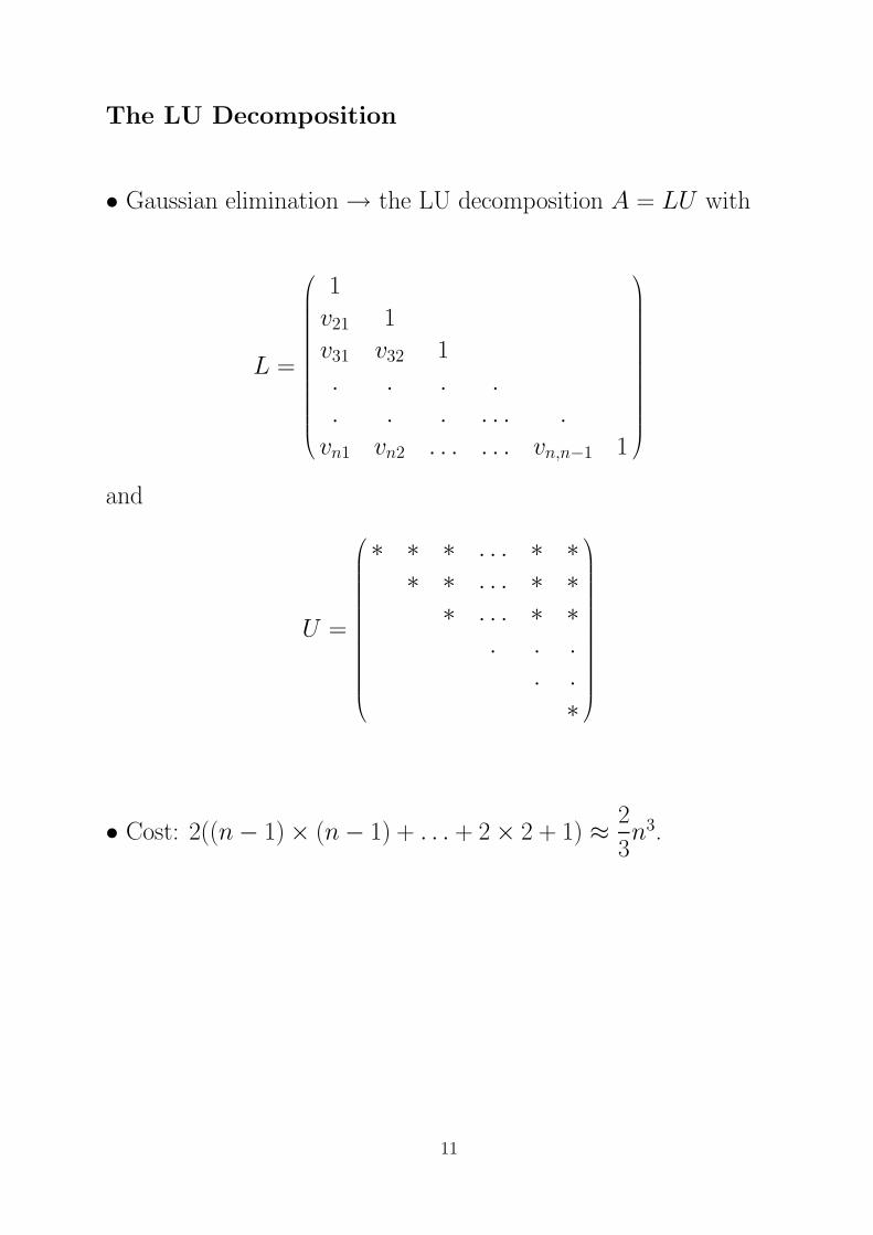
The LU Decomposition

• Gaussian elimination→ the LU decomposition A = LU with

L =

1

v21 1

v31 v32 1

. . . .

. . . . . . .

vn1 vn2 . . . . . . vn,n−1 1

and

U =

∗ ∗ ∗ . . . ∗ ∗∗ ∗ . . . ∗ ∗∗ . . . ∗ ∗

. . .

. .

∗

• Cost: 2((n− 1)× (n− 1) + . . . + 2× 2 + 1) ≈ 2

3n3.

11

// Returns the LU decomposition of A

function [L,U]=ludec(A);

[n,n]=size(A);

for k=1:n-1

A(k+1:n,k)=A(k+1:n,k)/A(k,k);

A(k+1:n,k+1:n)=A(k+1:n,k+1:n)-A(k+1:n,k)*A(k,k+1:n);

end

L=eye(n,n)+tril(A,-1);

U=triu(A);

endfunction

// Solves the linear system A*x=b via LU decomposition

function x=lusolve(A,b)

[L,U]=ludec(A);

y=lowtri(L,b);

x=uptri(U,y);

endfunction

12

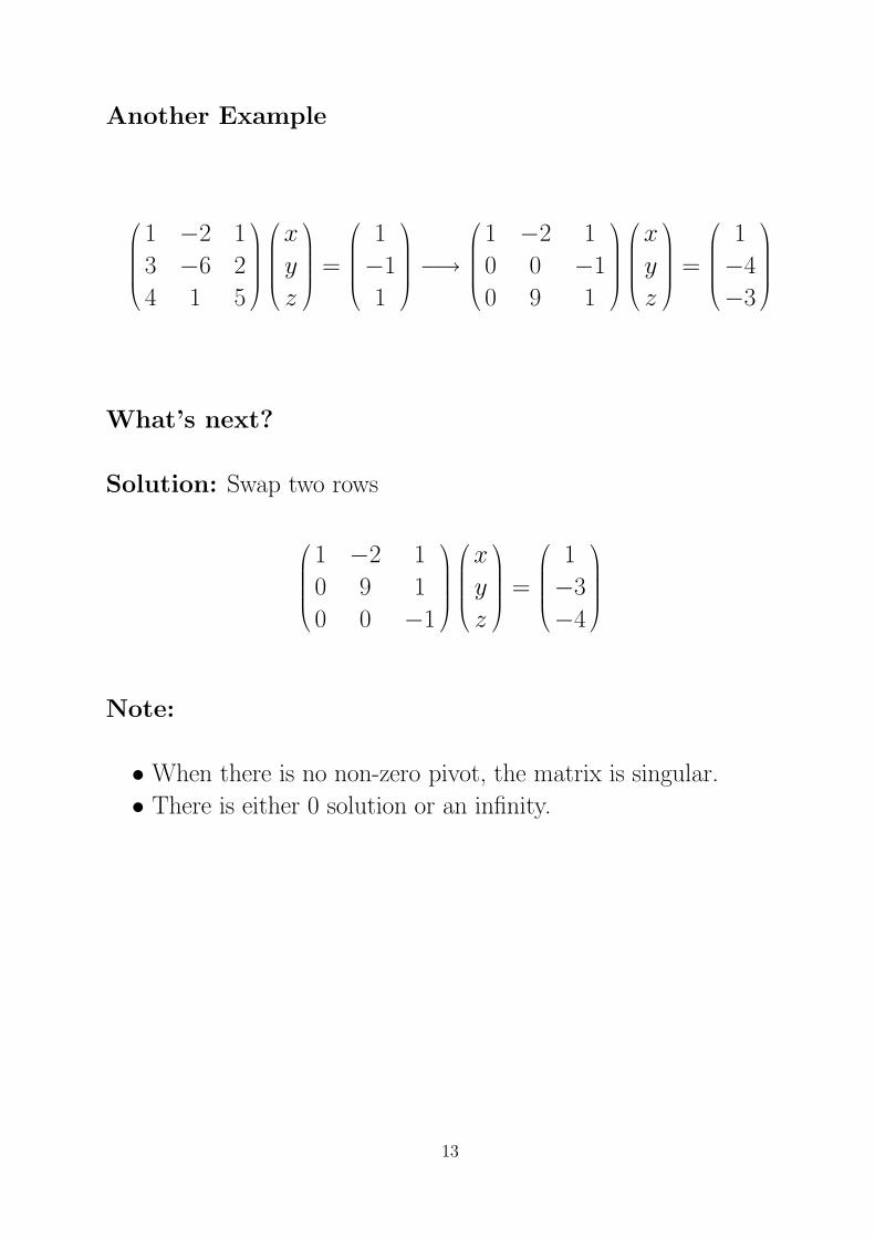
Another Example

1 −2 1

3 −6 2

4 1 5

x

y

z

=

1

−1

1

−→

1 −2 1

0 0 −1

0 9 1

x

y

z

=

1

−4

−3

What’s next?

Solution: Swap two rows

1 −2 1

0 9 1

0 0 −1

x

y

z

=

1

−3

−4

Note:

• When there is no non-zero pivot, the matrix is singular.

• There is either 0 solution or an infinity.

13

When LU fails...

Consider

A =

δ 1

1 1

=

1 01

δ1

δ 1

0 1− 1

δ

=⇒ Factorization is only possible when δ 6= 0.

Even Worse...

• Consider the system A~x =

δ + 1

2

• Its actual solution is ~x =

1

1

even when δ = 0.

• LU solution:

L~y = ~b

U~x = ~y

1 01

δ1

y1

y2

=

δ + 1

2

⇐⇒

y1 = δ + 1 ∼= 1

y2 = 2− y1

δ∼= −1

δ

δ 1

0 1− 1

δ

x1

x2

=

y1

y2

=⇒

x2 =y2

1− 1/δ∼= − 1/δ

− 1/δ= 1

x1 =y1 − x2

δ∼= 1− 1

δ= 0

14

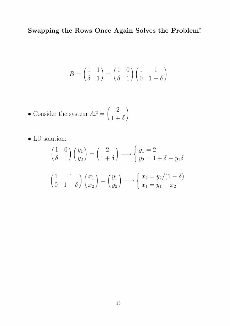
Swapping the Rows Once Again Solves the Problem!

B =

1 1

δ 1

=

1 0

δ 1

1 1

0 1− δ

• Consider the system A~x =

2

1 + δ

• LU solution:

1 0

δ 1

y1

y2

=

2

1 + δ

−→

y1 = 2

y2 = 1 + δ − y1δ

1 1

0 1− δ

x1

x2

=

y1

y2

−→

x2 = y2/(1− δ)

x1 = y1 − x2

15

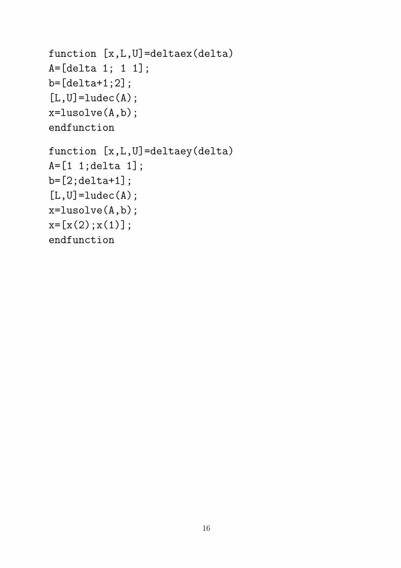
function [x,L,U]=deltaex(delta)

A=[delta 1; 1 1];

b=[delta+1;2];

[L,U]=ludec(A);

x=lusolve(A,b);

endfunction

function [x,L,U]=deltaey(delta)

A=[1 1;delta 1];

b=[2;delta+1];

[L,U]=ludec(A);

x=lusolve(A,b);

x=[x(2);x(1)];

endfunction

16

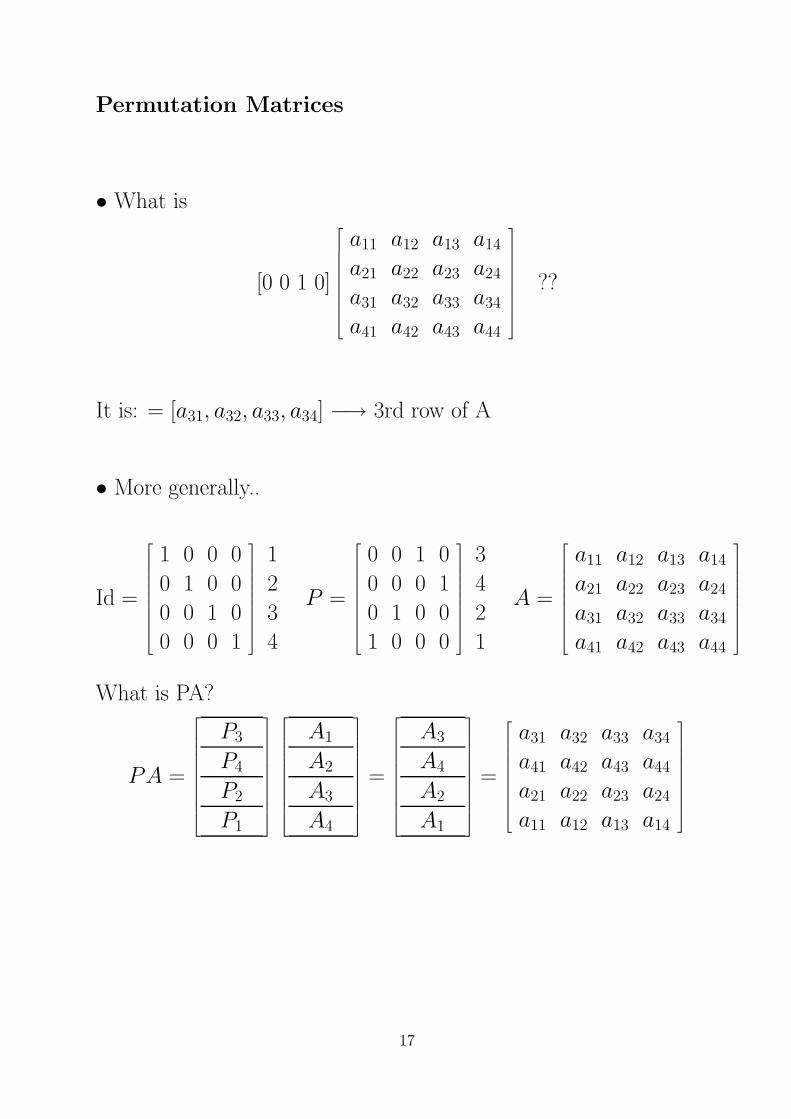
Permutation Matrices

• What is

[0 0 1 0]

a11 a12 a13 a14

a21 a22 a23 a24

a31 a32 a33 a34

a41 a42 a43 a44

??

It is: = [a31, a32, a33, a34] −→ 3rd row of A

• More generally..

Id =

1 0 0 0

0 1 0 0

0 0 1 0

0 0 0 1

1

2

3

4

P =

0 0 1 0

0 0 0 1

0 1 0 0

1 0 0 0

3

4

2

1

A =

a11 a12 a13 a14

a21 a22 a23 a24

a31 a32 a33 a34

a41 a42 a43 a44

What is PA?

PA =

P3

P4

P2

P1

A1

A2

A3

A4

=

A3

A4

A2

A1

=

a31 a32 a33 a34

a41 a42 a43 a44

a21 a22 a23 a24

a11 a12 a13 a14

17

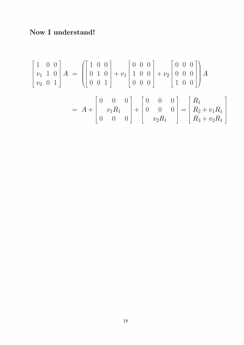
Now I understand!

1 0 0

v1 1 0

v2 0 1

A =

1 0 0

0 1 0

0 0 1

+ v1

0 0 0

1 0 0

0 0 0

+ v2

0 0 0

0 0 0

1 0 0

A

= A +

0 0 0

v1R1

0 0 0

+

0 0 0

0 0 0

v2R1

=

R1

R2 + v1R1

R3 + v2R1

18

Solving A~x = ~b

1. Compute L, U, P such that PA = LU

2. Note that PA~x = (LU)~x = P~b

2.1. Solve L~y = P~b

2.2. Solve U~x = ~y

In MATLAB:

[L,U,piv]=GEpiv(A); ← 2n3/3 flops

y=LTriSol(L,b(piv)); ← n2 flops

x=UTriSol(U,y); ← n2 flops

How much

does solving A~x = ~bi for i = 1 : k cost?

2

3n3 + 0(kn2) flops.

19

// Returns the LU decomposition of A with pivoting

function [L,U,piv]=ludecpiv(A);

[n,n]=size(A);

piv=[1:n];

for k=1:n-1

[mavx,r]=max(abs(A(k:n,k)));

q=r+k-1;

piv([k q])=piv([q k])

A([k q],:)=A([q k],:)

if A(k,k)~=0

A(k+1:n,k)=A(k+1:n,k)/A(k,k);

A(k+1:n,k+1:n)=A(k+1:n,k+1:n)-A(k+1:n,k)*A(k,k+1:n);

end

end

L=eye(n,n)+tril(A,-1);

U=triu(A);

endfunction

// Solves the linear system A*x=b via LU decomposition

// with pivoting

function x=lusolvepiv(A,b)

[L,U,piv]=ludecpiv(A);

y=lowtri(L,b(piv));

x=uptri(U,y);

endfunction

20

Another Example

1.0 0.33

0.33 0.11

x

y

=

−1

0

A

1 13

13

19

• Suppose two different processes give us two different numerical

solutions:

x1 =

−101

300

x2 =

−110

330

• We have

Ax1 =

−2

−0.33

Ax2 ≃

−1.1

0.0

• And the exact solution is x =

−100

300

• Which numerical solution is better?

21

Errors involved in solving linear systems

Let x be the numerical solution of Ax = b.

How good is x ?

Residual error

||b− Ax|| (or||b− Ax||||b|| )

Error in x

||x− x|| (or||x− x||||x|| )

Which one is a better error measure?

It depends, of course

=⇒ Polynomial fitting

=⇒ Pose fitting

22

Quantifying Errors: Norms and Distances

• How big is a vector ~x = (x1, ..., xn) ?

Norms:

||~x||1 = |x1| + · · · + |xn|

||~x||∞ = max{|x1|, · · · , |xn|}

||~x||2 =√

x21 + · · · + x2

n ≡ Euclidean norm

• How far are two points with positions ~x and ~y ?

Distances:

d1(~x, ~y) = ||~x− ~y||1

d∞(~x, ~y) = ||~x− ~y||∞

d2(~x, ~y) = ||~x− ~y||2 ≡ Euclidean distance

• Note: Norms induce distances. You can define distances without

norms.

• What are the level sets of the various norms?

||~x||2 = 1 ||~x||1 = 1 ||~x||∞ = 1

23

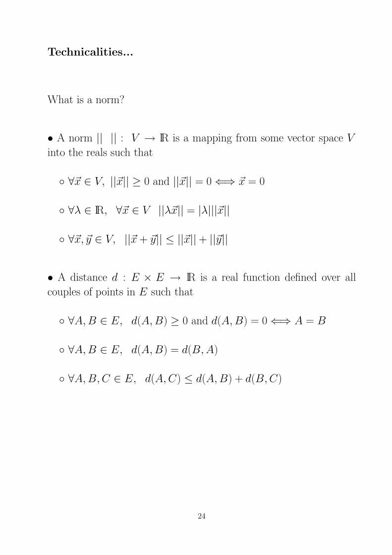
Technicalities...

What is a norm?

• A norm || || : V → IR is a mapping from some vector space V

into the reals such that

◦ ∀~x ∈ V, ||~x|| ≥ 0 and ||~x|| = 0⇐⇒ ~x = 0

◦ ∀λ ∈ IR, ∀~x ∈ V ||λ~x|| = |λ|||~x||

◦ ∀~x, ~y ∈ V, ||~x + ~y|| ≤ ||~x|| + ||~y||

• A distance d : E × E → IR is a real function defined over all

couples of points in E such that

◦ ∀A, B ∈ E, d(A, B) ≥ 0 and d(A, B) = 0⇐⇒ A = B

◦ ∀A, B ∈ E, d(A, B) = d(B, A)

◦ ∀A, B, C ∈ E, d(A, C) ≤ d(A, B) + d(B, C)

24

Theorem:

In IRn, all norms are equivalent, ie, if N1 : IRn → IR+ and N2 : IRn →IR+ are two norms, then there exist constants λ > 0 and µ > 0 such

that

∀~x ∈ IRn λN1(~x) ≤ N2(~x) ≤ µN1(~x)

• In particular

||~x||∞ ≤ ||~x||1 ≤ n||~x||∞

||~x||∞ ≤ ||~x||2 ≤√

n||~x||∞

• In plain English

−→ You can pick whichever norm is more convenient.

−→ Qualitatively, they give similar measures.

25

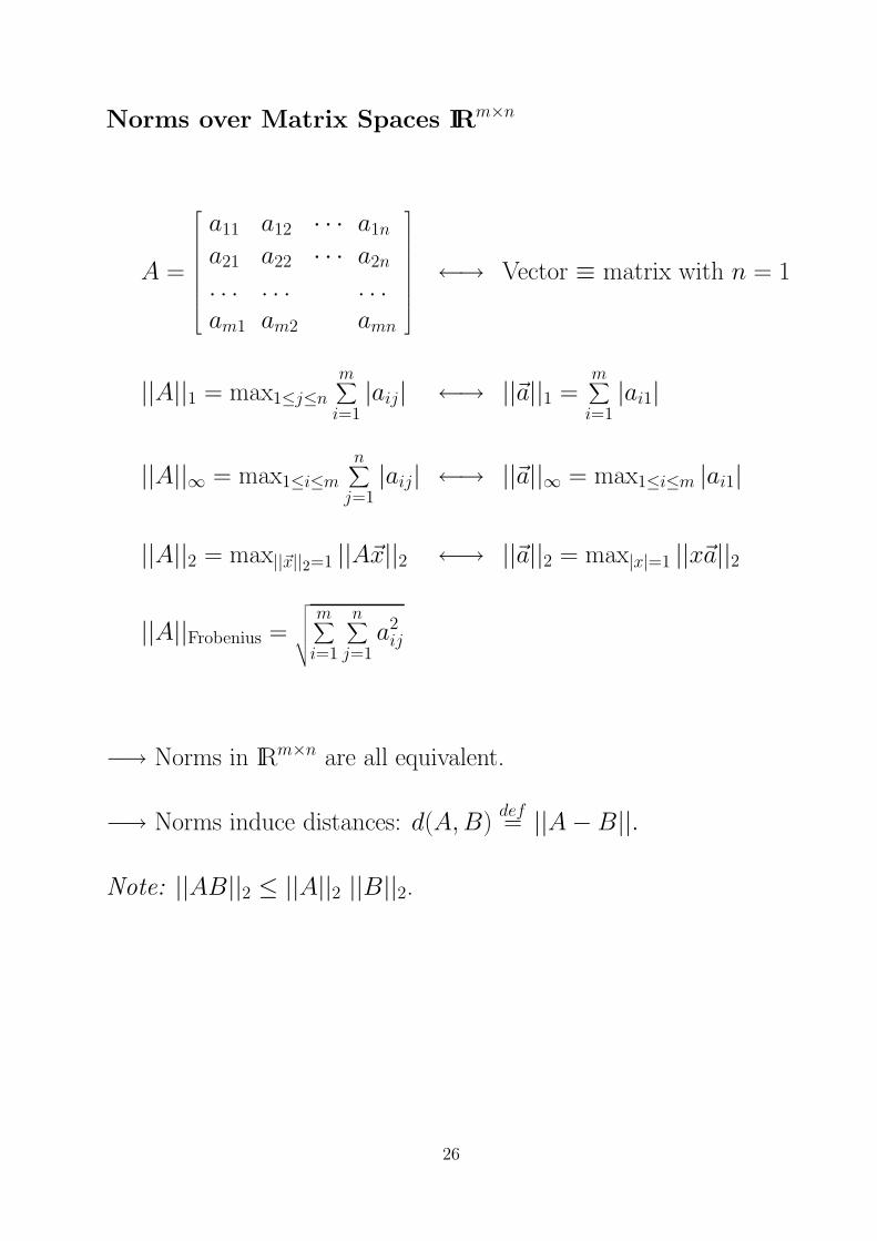
Norms over Matrix Spaces IRm×n

A =

a11 a12 · · · a1n

a21 a22 · · · a2n

. . . . . . . . .

am1 am2 amn

←→ Vector ≡ matrix with n = 1

||A||1 = max1≤j≤n

m∑

i=1|aij| ←→ ||~a||1 =

m∑

i=1|ai1|

||A||∞ = max1≤i≤m

n∑

j=1|aij| ←→ ||~a||∞ = max1≤i≤m |ai1|

||A||2 = max||~x||2=1 ||A~x||2 ←→ ||~a||2 = max|x|=1 ||x~a||2

||A||Frobenius =

√

√

√

√

√

m∑

i=1

n∑

j=1a2

ij

−→ Norms in IRm×n are all equivalent.

−→ Norms induce distances: d(A, B)def= ||A−B||.

Note: ||AB||2 ≤ ||A||2 ||B||2.

26

Floating-Point Errors

Assume floating-point arithmetic with numbers of the form

x = ± . b1b2 . . . br × βe with

L ≤ e ≤ U

0 ≤ bi ≤ β − 1

and define machine precision ε = 12β1−t .

Example: 3 digits, base 10, ε = 1210−2 = 5× 10−3

Theorem (Chap. 1):

|F l(x)− x||x| ≤ ε

Theorem (Chap. 5): For any matrix A ∈ IRm×n

||F l(A)− A||1||A||1

≤ ε.

Corollary: ||F l(A)− A|| ≤ ε||A|| .

Likewise: ||F l(AB)−AB|| ≈ ||A|| ||B|| .

What about errors in solving linear systems?

27

Condition number of a matrix

Define: κ1(A)def= ||A||1 ||A−1||1 is the condition number of A.

We have:

• κ1(A) ≥ 1,

• κ1(λA) = κ1(A),

• The larger κ1(A), the closer A is to being singular.

Theorem: If A ∈ IRn×n is non-singular, A~x = ~b, and εκ1(A) < 1,

then

• F l(A) is non-singular, and

• the solution of F l(A)x = F l(~b) verifies:

||x− ~x||1||~x||1

≤ εκ1(A) (1 +||x||1||~x||1

)

Note:

• This result has nothing to do with any algorithm.

• Similar results hold for the other norms.

28

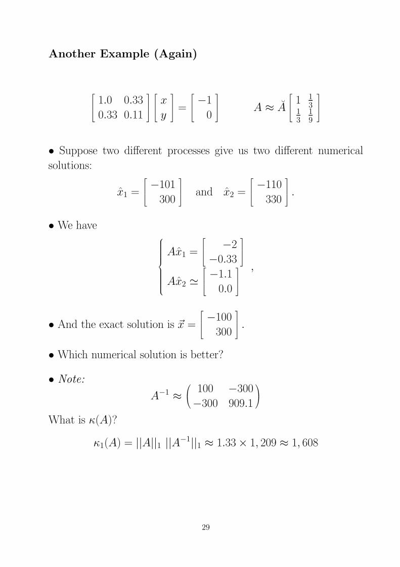
Another Example (Again)

1.0 0.33

0.33 0.11

x

y

=

−1

0

A ≈ A

1 13

13

19

• Suppose two different processes give us two different numerical

solutions:

x1 =

−101

300

and x2 =

−110

330

.

• We have

Ax1 =

−2

−0.33

Ax2 ≃

−1.1

0.0

,

• And the exact solution is ~x =

−100

300

.

• Which numerical solution is better?

• Note:

A−1 ≈

100 −300

−300 909.1

What is κ(A)?

κ1(A) = ||A||1 ||A−1||1 ≈ 1.33× 1, 209 ≈ 1, 608

29

Backward Stability

• If x is the solution to the problem A~x = ~b found by Gaussian

elimination, then

(A + E)x = ~b

for some matrix E such that ||E|| ≈ ε||A|| .

• Note: ||F l(A)− A|| ≈ ε||A||

• Corollary:

||Ax−~b|| ≈ ε||A|| ||x||

||x− ~x||||~x|| ≈ εκ(A)

30

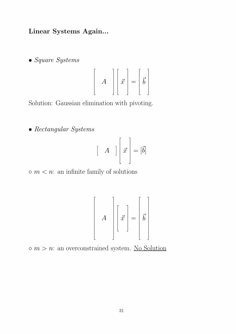
Linear Systems Again...

• Square Systems

A

~x

=

~b

Solution: Gaussian elimination with pivoting.

• Rectangular Systems

[

A]

~x

= [~b]

◦ m < n: an infinite family of solutions

A

~x

=

~b

◦ m > n: an overconstrained system. No Solution

31

Be Pragmatic!

If A~x = ~b is an overconstrained system without an exact solution,

find ~x that minimizes a reasonable error.

• Ex1: Minimize ||A~x−~b||21.

• Ex2: Minimize ||A~x−~b||22 ← LINEAR LEAST SQUARES.

Application: Data analysis: compute the parameters of a model

that best fits the data.

• Ex3:

f(x) = ax + b

• Ex4:

f(x) = anxn + · · · + a1x + a0

• Note: The Euclidean norm yields simple formulas for derivative

computation:

||~x||22 = (x21 + x2

2 + · · · + x2n) = ~x.~x = ~xT~x

32

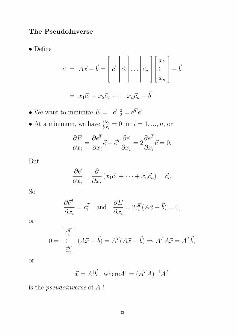
The PseudoInverse

• Define

~e = A~x−~b =

~c1 ~c2 . . . ~cn

x1...

xn

−~b

= x1~c1 + x2~c2 + · · ·xn~cn −~b

• We want to minimize E = ||~e||22 = ~eT~e.

• At a minimum, we have ∂E∂xi

= 0 for i = 1, ..., n, or

∂E

∂xi=

∂~eT

∂xi~e + ~eT ∂~e

∂xi= 2

∂~eT

∂xi~e = 0.

But

∂~e

∂xi=

∂

∂xi(x1~c1 + · · · + xn~cn) = ~ci,

So

∂~eT

∂xi= ~cT

1 and∂E

∂xi= 2~cT

i (A~x−~b) = 0,

or

0 =

~cTi

...

~cTn

(A~x−~b) = AT (A~x−~b)⇒ ATA~x = AT~b,

or

~x = A†~b whereA† = (ATA)−1AT

is the pseudoinverse of A !

33