
ARMAR-III: An integrated humanoid platform for sensory-motor control

Master ThesisFakultät Elektrotechnik und Informationstechnik
Nadia Barbara Figueroa Fernandez
3D Registration for Verification of Humanoid Justin’s UpperBody Kinematics.
Institut für RoboterforschungAbteilung Informationstechnik
IRF Referee: Prof. Dr. Uwe SchwiegelshohnIRF Referee: Dipl.-Inf. Oliver UrbannDLR Advisor: Florian SchmidtDLR Advisor: Dr. Haider Ali
March 12, 2012


Abstract
Humanoid robots such as DLR’s Justin were designed to interact with unknown environ-ments and cooperate with humans. To ensure safety and mobility they are built withlight-weight structures and flexible mechanical components. This light-weight design en-ables the robot to achieve a compliant behavior of the arm kinematic chain, with thedraw-back of having a low positioning accuracy at the TCP (Tool-Center-Point) end-poseof the hand. Torque sensors are used to approximate the deflections of the joints andcompensate the TCP end-pose errors. However, this approximation is insufficient due toremaining unidentified errors and flexibilities in the joints and links. The identification ofa maximum TCP end-pose error is essential for object manipulation and path planning.
This thesis proposes a verification routine for the identification of the maximum boundsof the TCP end-pose errors by using the on-board stereo vision system. The error identi-fication is based on the pose estimation of 3D point clouds of Justin’s hand using state-of-the-art 3D registration techniques.
A model of the hand is required for pose estimation. The hand’s CAD (Computer-Aided-Design) model does not accurately reflect the data observed by the stereo vision system,therefore we generate models of the hand by registering multiple 3D point clouds. Be-cause the hand is a self-occluding object a full model is not achievable. Partial models aregenerated by creating subsets of overlapping point clouds. We proposed a method for therejection of non-overlapping point clouds based on a statistical analysis of the depth values.The partial models are created by applying an extended metaview registration method tothe remaining subset of point clouds.
The registration of a random point cloud of the hand to the model generates an estimateof the TCP end-pose. This estimate is compared to the measured TCP end-pose obtainedby computing the forward kinematics of the arm using the joint angle measurements. Theverification routine consists in repeating this procedure with N -random poses. The boundsof the TCP end-pose errors are identified as the maximum translational and rotational er-ror from the set of random poses.
To evaluate the errors identified by using 3D registration, we implemented a marker-basedpose estimation method with the ARTrack IR Optical tracking system. This method re-quired a robust calibration of tracking targets to Justin’s head and hands. The errorsestimated by using this tracking system are considered as the ground truth. Experimentalresults showed that the estimated errors by using 3D registration are consistent with thisground truth. Therefore, our proposed verification routine is suitable for the bound iden-tification of Justin’s TCP end-pose errors. The identified bounds can be used to adjustthe obstacle clearance in path planning techniques. Unexpected collisions with the envi-ronment can be prevented by setting this clearance to a value higher than the maximumbound of the TCP end-pose errors.

AcknowledgementsFirst and foremost, I would like to express my sincere gratitude to my supervisors at DLR,Dr. Haider Ali and Florian Schmidt. This thesis would not have been possible withouttheir guidance and support.
I wish to thank my advisors at TU Dortmund, Oliver Urbann for his feedback and assis-tance and Prof. Dr. Uwe Schwiegelshohn for accepting to supervise this work.
I owe my deepest gratitude to my parents, Dr. Bertha Fernandez and Dr. Javier Figueroa.They have blindly believed in me and supported me with every decision I have taken inmy life.
I am grateful to my dear friends Marina, Cordelia, Jorge, Christina and Layla for theiremotional support and keeping me sane during this entire process. Even though we aremiles away, they will always be close to my heart.
Finally, I would like to thank Stefani Germanotta for inspiring me to never give up on mydreams.
Nadia Figueroa

Contents
1 Introduction 1
2 Data Acquisition and Processing 102.1 On-Board Stereo Vision System . . . . . . . . . . . . . . . . . . . . . . . . . 112.2 3D Point Cloud Processing . . . . . . . . . . . . . . . . . . . . . . . . . . . 162.3 Summary . . . . . . . . . . . . . . . . . . . . . . . . . . . . . . . . . . . . . 19
3 Pair-Wise Registration of 3D Point Clouds 203.1 Coarse Registration Evaluation . . . . . . . . . . . . . . . . . . . . . . . . . 22
3.1.1 Texture-based Correspondence . . . . . . . . . . . . . . . . . . . . . 223.1.2 Surface-based Correspondence . . . . . . . . . . . . . . . . . . . . . 243.1.3 Combined (Surface-Texture) Correspondence . . . . . . . . . . . . . 293.1.4 Local Feature Descriptor Comparison . . . . . . . . . . . . . . . . . 30
3.2 Fine Registration Evaluation . . . . . . . . . . . . . . . . . . . . . . . . . . 313.3 Summary . . . . . . . . . . . . . . . . . . . . . . . . . . . . . . . . . . . . . 33
4 Model Generation 344.1 Extended Metaview Registration Method . . . . . . . . . . . . . . . . . . . 374.2 6DOF Model Origin Estimation . . . . . . . . . . . . . . . . . . . . . . . . . 42
4.2.1 Estimates of the Absolute Origin from Extended Metaview Registration 434.2.2 Computation of the Absolute Origin of the Model . . . . . . . . . . 47
4.3 Model Evaluation . . . . . . . . . . . . . . . . . . . . . . . . . . . . . . . . . 494.3.1 Construction of Synthetic Models . . . . . . . . . . . . . . . . . . . . 494.3.2 Visibility Consistency Measures . . . . . . . . . . . . . . . . . . . . . 52
4.4 Summary . . . . . . . . . . . . . . . . . . . . . . . . . . . . . . . . . . . . . 56
5 Pose Estimation by using the IR Tracking System 575.1 ART Set-up for pose estimation . . . . . . . . . . . . . . . . . . . . . . . . . 595.2 Calibration of targets to Justin . . . . . . . . . . . . . . . . . . . . . . . . . 61
5.2.1 Center of Rotation Estimation . . . . . . . . . . . . . . . . . . . . . 635.2.2 Axes of Rotations Estimation . . . . . . . . . . . . . . . . . . . . . . 735.2.3 Frame Estimation . . . . . . . . . . . . . . . . . . . . . . . . . . . . 78
5.3 Error Identification . . . . . . . . . . . . . . . . . . . . . . . . . . . . . . . . 835.4 Method Limitations . . . . . . . . . . . . . . . . . . . . . . . . . . . . . . . 86
iii

5.5 Summary . . . . . . . . . . . . . . . . . . . . . . . . . . . . . . . . . . . . . 87
6 Pose Estimation by using 3D Registration 886.1 Error Identification . . . . . . . . . . . . . . . . . . . . . . . . . . . . . . . . 916.2 Error Evaluation Method . . . . . . . . . . . . . . . . . . . . . . . . . . . . 926.3 Method Limitations . . . . . . . . . . . . . . . . . . . . . . . . . . . . . . . 946.4 Random Pose Generator . . . . . . . . . . . . . . . . . . . . . . . . . . . . . 976.5 Experimental Results . . . . . . . . . . . . . . . . . . . . . . . . . . . . . . . 99
6.5.1 Environment-1 . . . . . . . . . . . . . . . . . . . . . . . . . . . . . . 1036.5.2 Environment-2 . . . . . . . . . . . . . . . . . . . . . . . . . . . . . . 1056.5.3 Environment-3 . . . . . . . . . . . . . . . . . . . . . . . . . . . . . . 1076.5.4 Environment-4 . . . . . . . . . . . . . . . . . . . . . . . . . . . . . . 1096.5.5 Environment-5 . . . . . . . . . . . . . . . . . . . . . . . . . . . . . . 1116.5.6 Overall Performance . . . . . . . . . . . . . . . . . . . . . . . . . . . 113
6.6 Summary . . . . . . . . . . . . . . . . . . . . . . . . . . . . . . . . . . . . . 114
7 Application: Bound-Identification of Justin’s TCP Errors 115
8 Conclusions 119
A Brief description of algorithms 122A.1 Kd-tree for nearest neighbor search . . . . . . . . . . . . . . . . . . . . . . . 122A.2 SIFT (Scale Invariant Feature Transforms) Algorithm . . . . . . . . . . . . 123A.3 Principal Component Analysis . . . . . . . . . . . . . . . . . . . . . . . . . 125A.4 Automatic Extended Metaview Approach . . . . . . . . . . . . . . . . . . . 126
Bibliography 126
iv

Chapter 1
Introduction
The complex humanoid mobile robot rollin Justin of the Institute of Robotics and Mecha-tronics at DLR (German Aerospace Center) [1][2] is composed of preliminary works of theinstitute, namely the DLR Light Weight Robot (LWR) and the DLR Hand II. To emulatehuman-like mobility, Justin has a torso based on the LWR technology and two (left andright) light-weight robot arms and hands (Fig.1.1).
Figure 1.1: DLR’s rollin Justin
Light-weight robots do not follow the same design concept of typical industrial robots.Industrial robotic arms are stiff and heavy manipulators that can obtain high position-ing accuracy and repeatability. They are mainly used for repetitive positioning tasks inwell structured and known environments. On the other hand, light-weight robots aremanipulators built with light-weight structures and joints with mechanical compliances
1

2 CHAPTER 1. INTRODUCTION
and flexibilities. They are designed to interact with unknown environments and humansin application areas such as service robotics, space robotics, medical robotics, telepresenceand virtual reality. However, the skillful mobility and compliant interaction enabled by theLWR design also causes low positioning accuracy at the Tool-Center-Point (TCP) end-poseof the hands. This low positioning accuracy is produced by unidentified errors, compliancesand elasticities in the joints and links. It is reflected as translational and rotational errorsat the TCP end-pose. The impact of these errors is illustrated with a simple kinematicchain in Fig.1.2.
Figure 1.2: Bounds of the TCP end-pose errors ej = (ex, ey, ez, eθ) affected by joint/link uncer-tainties
The end-pose error ej = (ex, ey, ez, eθ) of a commanded pose pj is caused by uncertaintiesin the measured angles θ0, θ1, θ2. This is represented in the following equation:
pj = f(θj0 , θj1 , .., θjn) + ej (1.1)
Where f is the forward kinematics, θji are the measured joint angles and ej are the errorsof the end pose of this kinematic chain. With the identification of ej , one can furtheranalyze the kinematic chain and map these errors to joint space. This is represented by asimplified equation:
θji = f−1(pj) + ejθ (1.2)
Where f−1 is the inverse kinematics and ejθ are the errors mapped into joint space. Thisestimation is not straight-forward and is out of the scope of this thesis.
The kinematic chain of Justin’s LWR arms was designed with seven degrees of freedomto achieve a similar kinematic redundancy as the human arm. This redundancy enablesJustin to reach the same TCP end-pose with an infinite number of joint positions. Whenreaching a commanded pose pj , the set of values for each joint angle θji calculated by theinverse kinematics f−1 may be an infinite number of combinations.

3
We commanded Justin’s right arm to reach a fixed TCP end-pose with three randomkinematic joint configurations. This is illustrated in Fig.1.3.
Figure 1.3: Same commanded TCP pose, different kinematic configurations. (top row) left cameraview of the TCP from the head mounted stereo system, (bottom row) kinematic configuration usedfor each TCP pose
Ideally, all of the kinematic configurations should reach the same TCP end-pose. However,as can be seen in Fig.1.4, the arm reaches three different TCP end-poses.
Figure 1.4: Overlapped images of same commanded TCP pose, different reached poses. (noticethe finger areas and the overall blurred effect on the hand)

4 CHAPTER 1. INTRODUCTION
The identification of these TCP end-pose errors is essential for successful path planningand object manipulation tasks. Therefore, the main goal of this thesis is the identificationof the maximum bounds of these errors. As stated earlier, these errors are caused by theinherent flexibility in the LWR design. Mechanical flexibility exists due to the use of com-pliant transmission elements and the reduction of mass of moving links using lightweightmaterial and slender designs. These flexibilities introduce static and dynamic deflectionsbetween the position of the joints and the end-pose of the hands [3]. An approximation of ajoint’s deflection can be obtained by using the torque sensors integrated in each joint. Dur-ing the assembly of the arm the stiffness of the gears and links was identified. With thesestiffness values and the load and torque measurements, joint deflections can be estimated.In Fig.1.5 the configuration of a joint of the arm is illustrated.
Figure 1.5: The mechatronic joint design of the LWR
The joint drive has a highly accurate position sensor attached to it. On the output ofthe gear unit a less accurate position sensor and a torque sensor are attached to it as well.The position of the joint is computed by combining the motor side high precision positionsensor with the link-side torque sensor. This position describes the origin of the link. Areduced flexible joint model is used to estimate the end point of the link, which is connectedto the next joint. Therefore, the measured joint positions consider an approximation ofthe joint’s deflection. However, this approximation is not enough to identify the absoluteerrors in the joints and links.
On a complex system like the DLR’s rollin Justin there are several error models andcalibration procedures for different parts of the kinematic chain. Our goal is not to cre-ate a new calibration procedure, but to verify and check the plausibility of the existingones. The state-of-art of verifying these error models and calibrations is quite manual, soan easy and automatic procedure to obtain the bounds of the TCP errors that can ver-ify these models is required. This procedure has to be as stable and trustworthy as possible.

5
The verification of Justin’s kinematic chains is based on robot arm calibration concepts.Several configurations exist for robot arm calibration, based on measuring the 3D poseof the end-effector. In [4] the open loop, closed loop and implicit loop configurations arereviewed. In an open loop configuration the manipulator is not in contact with the envi-ronment. The closed loop configuration uses physical constrains on the end-effector, thusforming a closed loop with the ground. The implicit loop configuration uses a calibratedsensory system that measures the 3D coordinates of a certain point on the end-effector ofthe uncalibrated robot, this system is replaced by a prismatic leg which represents a 6DOFjoint. This joint will provide 3D coordinates, thus resulting in a closed loop mechanism,as illustrated in Fig.1.6.
Figure 1.6: Simplified Representation of an Implicit Loop Configuration
In [5], Khalil introduces a variant of implicit loop closing, instead of measuring the 3Dpositions of the end-effector, distance measures are used. So instead of using sensory sys-tems, geometric constrains are applied on the robot with the environment and only thejoint variables are used. In this approach, the end-effector of the robot is constrained tolie on the same plane. Touch or tactile sensors can be used to measure these variationsusing plane equations or coordinates to normal of the planes. In earlier work, the use oftouch or tactile sensors was preferred over vision systems due to the lack of accuracy. Inthe state-of-art, tools like the Open Source Point Cloud Library [6] (PCL) (Fig.1.7) existwhich enable the processing and analysis of 3D representations of a scene generated fromstereo data or any other depth sensor (ie. Kinect, Time-Of-Flight).
Figure 1.7: Open Source Point Cloud Library

6 CHAPTER 1. INTRODUCTION
Our verification procedure is based on the implicit loop configuration using a sensorysystem, mainly for two reasons:
• When generating measurements by contacts to the environment as in the closed loopconfiguration or the implicit loop variant proposed by Khalil [5], this would introduceexternal forces acting on the arm, consequently introducing additional deflections tothe joints of the kinematic chain. We want to avoid introducing any kind of externalerrors to the kinematic chain, therefore the implicit loop configuration is the mostsuitable for this procedure.
• Justin is equipped with an on-board stereo vision system. This system is calibrated tothe kinematic chain of the arms. Thus, 3D representations of the hands can be createdand their pose w.r.t. the arm’s coordinate system can be estimated. Additionally,we want to avoid the limitation of Justin’s mobility, the procedure should not bedependent on a specific external sensing device. By using the on-board stereo systemit can be possible to run this procedure in any room or lab.
The 3D representations extracted from the stereo vision system are called 3D point clouds.A point cloud is a set of points p ∈ P , where p has six coordinates p = (x, y, z, r, g, b). Thesecoordinates represent the position of that point w.r.t. coordinate frame of the vision sys-tem and it’s color values. The complete set of points P is the 3D description of the surfaceof the object or scene seen by the sensor. The pose of one object (represented by a pointcloud) w.r.t. another is estimated by registration. The 3D registration problem is now acommon problem in robotics. From solving hand-eye calibration to generating 3D mod-els from multiple data sets to estimating the pose of objects within a scene; all of theseproblems rely on one solution, which is to find the transformation between two coordinatesystems or sets of 3D points. Numerous solutions are proposed to solve the 3D registrationproblem. It is an interesting and challenging problem, due to the fact that the point-wisecorrespondences between the two datasets are unknown. In this work, we review and eval-uate the state-of-the-art techniques for 3D registration.
We propose a procedure for Justin to self-verify its upper body kinematic chains basedon 3D registration techniques using the on-board state-of-the-art stereo vision system.Verification and calibration procedures using vision sensors have been used for industrial,medical and personal robotic applications. Lorsakul et al. [7] estimate the pose betweena dental tool for implant surgery and a 3D position sensor. They compute rigid transfor-mations between point clouds of measurements and estimated poses, using singular valuedecomposition (SVD). They use markers to identify the tool. In an industrial scenario,Teconsult has developed a calibration procedure named ROSY (Robot Optimization SYs-tem)1. ROSY estimates the accuracy of the end pose of industrial arms. The robot’skinematic errors are measured by mounting a pair of digital cameras to the end-effectorand identifying the pose of a calibration sphere with different arm kinematic configura-tions. The most recent work in personal robotics is aimed at a self-calibration procedurefor Willow Garage’s PR2 robot. Pradeep et al [8] use measurements from kinematic chains,
1Teconsult Precision Robotics. Robot Optimization System (ROSY). http://www.teconsult.de/

7
stereo cameras, monocular cameras and tilting lasers to estimate the robot’s joint offsetsand sensor locations. The use of checkerboard targets is required for their calibration pro-cedure. All of these methods require either external calibrated tracking systems, markers,checkerboard patterns or external sensory systems.
Our proposed method is reproducible and avoids any human interaction or external lim-itation that would disable the robot of its mobile essence. We compute the bounds ofthe TCP errors of Justin’s kinematic chain by estimating the pose of the hand in severalkinematic configurations. To implement such a procedure with 3D registration, a modelof the hands is required. 3D CAD models of the hands were generated in the design andmanufacturing stage, however these do not accurately reflect the data observed by theactual sensing device. This can be seen in Fig.1.8. In order to accurately estimate a posewith the proposed method, a model of the hand has to be created with the 3D point cloudsgenerated from the stereo vision system.
Figure 1.8: 3D point cloud of the hand generated from stereo vision system vs. 3D point cloudof the CAD Model (notice the CAD model: has missing components, represents the fingers ascompletely rigid components and has no color information)
To evaluate our proposed pose estimation method, we develop a marker-based pose estima-tion method using retroreflective tracking targets and an infrared optical tracking systemdeveloped by Advanced Realtime Tracking GmbH2. This technology is used in various fieldssuch as virtual reality, motion capture, industrial measurement, medical applications, eyetracking and robot research and development. In the latter, ART systems are mountedand calibrated for the localization of autonomous robots, limb positions and targets forrobot grasping and manipulation. We calibrate robust passive targets to Justin’s head andhand. The 6D pose of these targets is computed by a calibrated system of four ARTrack3cameras mounted in Justin’s Lab. The pose estimated by this system is used as a groundtruth to evaluate the feasibility of our method.
2ARTrack tracking system. http://www.ar-tracking.com/products/tracking-systems.html

8 CHAPTER 1. INTRODUCTION
The outline of this thesis is depicted as a roadmap in Fig.1.9.
Figure 1.9: Thesis Outline. (arrows indicate required reading order, Chapter 5 is independent fromthe 3D registration techniques)

9
The first three chapters are dedicated to the data acquisition, processing and registrationtechniques used for our proposed pose estimation method based on 3D registration. Thefollowing two chapters address the pose estimation of Justin’s hand. The first of thesechapters describes the generation of our ground truth with the implementation of a poseestimation method by using the ARTrack system. The second presents our proposed poseestimation approach using 3D registration and it’s evaluation w.r.t. the ground truth. Thefinal chapter is the detailed description of the verification routine used to identify thebounds of Justin’s TCP errors. The key contributions of this work are the following:
• A model generation method for self-occluding objects is proposed.
• We propose a verification procedure using pose estimation by 3D registration, toestimate the bounds of the TCP errors on Justin’s upper body kinematic chains.• We implement a marker-based pose estimation method using the ARTrack IR Opticaltracking system to evaluate our own.

Chapter 2
Data Acquisition and Processing
Our pose estimation method is based on aligning sets of 3D points, called 3D point clouds.3D point clouds are representations of the world viewed by a sensor. Each point p of a 3Dpoint cloud has (x, y, z) coordinates relative to the fixed coordinate system of the originof the sensor. Depending on the sensing device the point p can additionally have colorinformation such as (r, g, b) values. 3D point clouds are generated from depth images ordepth maps. In a depth image, each pixel has a depth value assigned to it. These depthvalues are the distances of surfaces in the world to the origin of the camera. This resultsin a 2.5D representation of the world. This representation can be easily converted to a3D representation using the known geometry of the sensor. The most common approachesfor acquisition of depth images in robotic applications have been: Time-of-Flight (TOF)systems and triangulation-based systems [9].
TOF systems emit signals (ie. sound, light, laser) and measure the time it takes for thesignal to bounce back from a surface. Sensors such as LIDAR (Light Detection and Rang-ing), radars, sonars, TOF cameras and Photonic-Mixing-Device (PMD) cameras are partof this category. Triangulation-based systems measure distances to surfaces by matchingcorrespondences viewed by two sensors. These two sensors need to be calibrated w.r.t.each other. Stereo Vision Systems lie in this category. A new category of depth acquisitionsystems has grown popular in robotic applications since the launch of the Kinect sensor1. Itconsists of an infrared laser projector combined with a monochrome CMOS sensor, whichcaptures video data in 3D. The technology is called light coding2 and it is a variant ofimage-based 3D reconstruction.
Justin is equipped with a head mounted pair of calibrated stereo cameras, so we use thistriangulation-based system to generate our 3D point clouds.
1"Project Natal" 101". Microsoft. June 1,20092" c© 2010 PrimeSense Ltd. | FAQ". Primesense.com.
10

2.1. ON-BOARD STEREO VISION SYSTEM 11
2.1 On-Board Stereo Vision SystemStereo vision systems emulate binocular human behavior [10]. Therefore, the perception ofdepth is reconstructed with two calibrated cameras [11]. To mathematically represent theperception of each camera, the pinhole camera model is used. This is the most simplifiedmodel of a camera. It is based on modeling the lens of the camera as a pinhole (centerof projection) that lets through light rays that intersect a specific point in space and areprojected to an image plane [10], this is illustrated in Fig.2.1.
Figure 2.1: Camera pinhole model: A pinhole lets through light rays that intersect with objects inspace (depicted as the star), the projection of these rays to the image plane form the image. (Thisillustration is based on the camera pinhole model presented in [10])
Where f is the camera’s focal length and Z is the distance from the camera to the object.X is the length of the object and x is the length of the object in the image plane, whichby similar triangles -x/f = X/Z can be computed as follows:
− x = fX
Z(2.1)
Bradski and Kaehler [10], state that by swapping the pinhole and the image plane anequivalent camera pinhole model is obtained, which is easier to draw and describe math-ematically. A new frontal image plane is generated. The size of the object in this imageplane is the same as the old one and it is the same distance f to the pinhole plane. How-ever, the object is no longer upside down and the relationship by similar triangles is nowx/f = X/Z . This is illustrated in Fig.2.2.
Figure 2.2: Pc in space is projected to p on the image plane by a ray passing through the centerof projection O (This illustration is based on the projected camera pinhole model presented in [10])

12 CHAPTER 2. DATA ACQUISITION AND PROCESSING
Where f = (fx, fy) is the focal length of the camera, Pc = (X,Y, Z) is the reflected pointto the camera in camera coordinate frame, p = (u, v, f) is the resulting point on the imageplane and c = (cx, cy) is the principal point, which is the point where the principal rayintersects the image plane. With this simple model the pixel coordinates (u, v) of p on theimage plane corresponding to point Pc can be computed as follows:
u = fxX
Z+ cx (2.2)
v = fyY
Z+ cy (2.3)
This mapping between Pc and p can be computed by a transformation matrix A thatrepresents the intrinsic parameters of the camera. A is conformed of the focal length(fx, fy), principal points (cx, cy) and skew (defines the angle between the x and y pixelaxes):
A =
fx skew cx0 fy cy0 0 1
(2.4)
Therefore, by normalizing the X and Y coordinates of Pc as Xn = X/Z and Yn = Y/Z,they are mapped to pixel coordinates (u, v) as follows:uv
1
= A
Xn
Yn1
(2.5)
The extrinsic parameters of a camera describe the transformation of a point in the cameracoordinate system to a world coordinate system. The standard camera calibration proce-dure consists of finding the intrinsic/extrinsic parameters that relate the 3D coordinatesof control points and their image plane projections [12]. These control points are generallythe corners of the line crossings (edges) of planar chessboard patterns. Heikkil and Silven[13] developed a four step procedure for computing the intrinsic parameters. It uses ex-plicit calibration methods for mapping the 3D coordinates to the image coordinates andan implicit approach for image correction. It is implemented in OpenCV [10]. A similarapproach was implemented by Bouguet3 in a matlab calibration toolbox. The DLR Cal-ibration Toolbox (DLRCalLab)4 follows the same approach, but offers an improved finalaccuracy compared to the standard methods. Instead of using the a priori grid dimen-sions of the calibration pattern, these are parametrized and optimal calibration results areachieved disregarding the inaccuracies in the given grid dimensions [14]. It also deals withthe inaccuracies caused by imperfect planar patterns by applying concurrent optimizationof scene structure together with the intrinsic parameters [15].
3J.Y. Bouguet. Camera calibration toolbox for matlab http : //www.vision.caltech.edu/bouguetj/calibdoc/4K.H. Strobl. DLR CalLab and CalDe - The DLR Camera Calibration Toolbox.
http://www.dlr.de/rm/desktopdefault.aspx/tabid-3925/

2.1. ON-BOARD STEREO VISION SYSTEM 13
These calibration methods are extended to stereo systems. In stereo calibration the intrin-sic/extrinsic parameters of each camera are computed, as well as the rigid transformationbetween them. A simple stereo system is a constellation of two cameras having paralleloptical axes5 and separated by a baseline b, which is perpendicular to the line of sight ofthe cameras. A simple stereo rig model is illustrated in Fig.2.3.
Figure 2.3: Simplified stereo rig pinhole model (This illustration is based on the stereo rig modelpresented in [10])
The on-board stereo vision system is calibrated with the DLRCalLab. The left and rightimages (780x580) (Fig.2.4) are obtained via the SensorNet Library [16], which provides asmall and fast mechanism for distributing real time streaming data. Our stereo system hasa focal length of f = (732.5, 732.2) in pixels and a baseline of b = 0.05m. These parametersyield to a horizontal Field Of View (FOV) of 32 ◦ and vertical FOV of 20 ◦.
Figure 2.4: Left and Right Stereo Images of Justin’s right hand
5This is an assumption taken for a simplified stereo model, generally these axes are not required to beparallel.

14 CHAPTER 2. DATA ACQUISITION AND PROCESSING
Once the geometry of the stereo system is known, triangulation can be applied to thestereo images. As described by Bradski and Kaehler [10], after undistorting and rectifyingthe images, corresponding features between the left and right images are found. Thisgenerates a disparity map, where the disparities (d) are the differences in the x-coordinatesof corresponding features in each image plane. This disparity map is then converted to adepth map. Assuming the simplified stereo model (Fig.2.3), depth values (z) are computedusing similar triangles:
z = fb
d(2.6)
Where f is the focal length of the stereo camera and b is the baseline (distance between leftand right cameras). The important step in creating depth maps is stereo correspondence. Awide range of dense stereo algorithms have been developed [17]. These can be classified intolocal and global stereo correspondence algorithms. The local algorithms are based on find-ing disparities on intensity values within a finite window. The sum-of-squared-differences(SSD) is the traditional stereo correspondence algorithm. In OpenCV [10] a stereo corre-spondence algorithm is implemented similar to the one introduced by Konolige [18]. It usessmall sum-of-absolute-differences (SAD) windows to find correspondences. This approachis widely used in the robotics community, because of its availability and inexpensive com-putation. However, local algorithms assume constant disparities within a window. Theyconsider smoothness implicitly by aggregating support, this leads to blurred object bound-aries. Global algorithms make explicit smoothness assumptions, by finding disparities thatminimize a cost function that combines data and smoothness. Graph Cuts [19] and BeliefPropagation [20] are part of this category. These methods are effective but computation-ally inefficient. Hirschmüller [21] proposed a Semi-Global Matching (SGM) algorithm thatperforms pixel-wise matching based on Mutual Information and the approximation of aglobal smoothness constraint. The global cost calculation can be efficiently performed ina time linear to the number of pixels and disparities. Our disparity maps are generatedwith this approach, but using a Census pixel-matching method based on a Non-parametriccost [22]. The output is a 2.5D image, containing color (RGB) and depth information perpixel.
In Eq.2.6, it can be seen that the calculated depth values (z) are highly dependent on thedisparities (d). In fixed baseline stereo systems, the depth error grows quadratically withdepth [23]. This means that the accuracy of a stereo vision system is much higher in closerranges than in far. Thus the depth error in stereo, as described by Chang and Chatterjee[24], is shown to be:
∆z = z2
bf·∆d (2.7)
In Eq.2.7, ∆z is the depth error, z is the depth, b is the baseline, f is the focal length inpixels and ∆d is the disparity accuracy. ∆d is the matching error in pixels, we use 0.5 forthis value, it is the average pixel error for the applied SGM approach.

2.1. ON-BOARD STEREO VISION SYSTEM 15
In Fig.2.5, an illustration of the incrementing depth resolution in a standard fixed baselinestereo system is shown.
Figure 2.5: Standard Stereo with variable Depth Resolution (Illustration based on variable stereoresolution depicted in [23])
In Table 2.1 the depth resolutions corresponding to our on-board stereo system are shown.The reach of Justin is limited to approx. 0.6m from the origin of the stereo system in thedirection of the optical axis, so our depth values have a minimum accuracy of 5mm. Thisresolution will be shown to be sufficient for our pose estimation method.
Table 2.1: Stereo Depth Resolution
Depth (Z) [m] 0.05 0.1 0.3 0.5 0.6 1 1.5Resolution (∆z) [cm] 0.0034 0.013 0.12 0.33 0.49 1.35 3.05

16 CHAPTER 2. DATA ACQUISITION AND PROCESSING
2.2 3D Point Cloud ProcessingThe geometric mapping of 2.5D image coordinates to 3D coordinates in a stereo system isof perspective type [16]. This means that the sensor is described by the pinhole cameramodel. All rays intersect at one focal point (Fig.2.6).
Figure 2.6: Perspective Geometry (This illustration is based on the perspective geometry modelpresented in [16])
We assume that the coordinates of the depth image are equidistant w.r.t. the imagecoordinate system. Therefore, the physical pixel coordinates ui, vj of a depth pixel zij arecomputed using the offsets (which are the principal points w.r.t. the image plane origin)u0, v0 and the pixel increments ∆u,∆v [16].
ui = u0 + i ·∆u (2.8)
vj = v0 + j ·∆v (2.9)
The mapping of the Cartesian point pij for the perspective sensors is given by:
pij(xij , yij , zij) =
zij · uizij · vjzij
(2.10)
The depth and color (r, g, b) coordinates of each pixel (ui, vj) from the 2.5D image obtainedby the SGM stereo processing algorithm are mapped by Eq.2.10 to generate a 3D pointcloud P , where p = {x, y, z, r, g, b} for p ∈ P .

2.2. 3D POINT CLOUD PROCESSING 17
An example of a 3D point cloud generated from Justin’s on-board stereo vision is shownin Fig.2.7.
Figure 2.7: Dense 3D point cloud. (top) front view (bottom) side view

18 CHAPTER 2. DATA ACQUISITION AND PROCESSING
The region of interest in the point clouds are Justin’s hands. Because Justin’s reach isaround 0.6m in the z-direction from the sensor origin, we apply a pass-through filter [25]at 0.7m to cut-off any 3D points related to the background.
The extracted point cloud of the hand is quite dense. As any other depth sensor, stereosystems are subject to noise. There could be phantom points at depth discontinuities, mixedpixels, errors due to thin structures, specular reflections and color boundaries [26]. Tanget. al [26] compare several algorithms for detecting mixed pixels and depth discontinuities.They found that even though most algorithms had their limitations, the surface normalbased algorithms had the best performance. The methods they compare are based on thetriangulation of 3D point clouds and only solve the problem for mixed pixels and depthdiscontinuities. To avoid the triangulation step and remove all points in sparse densityareas (noise) regardless of the error type, Rusu et al. [27] [25] proposed a solution basedon the statistical analysis on the neighborhood P ki of each point pi ∈ P . It is based on thecomputation of the distribution of point distances from a query point to its neighboringpoints. For each point pi, the mean distance from it to all its neighbors pkj ∈ P ki
6 iscomputed. By assuming that the resulted distribution is Gaussian with a mean and astandard deviation, all points whose mean distances are outside an interval defined by themean distance (µk) and standard deviation (σk) from their neighborhood and a densityrestrictive threshold (dthres) are considered as outliers and removed from the point cloud.This procedure is applied to every point pi ∈ P as follows:
P f = {pi ∈ P |(µk − dthres · σk) ≤ d̄(pi, pkj ) ≤ (µk + dthres · σk)} (2.11)
Where d̄(pi, pkj ) is the mean Euclidean distance of a query point (pi) to its neighboringpoint (pkj ) and (µk+/-dthres ·σk) are the minimum and maximum distance thresholds. Afterapplying this filter, the resulting point cloud P f is still dense. To reduce computation timeand create a uniform density on the point cloud, we apply a Voxel Grid filter [25]. This filtercreates a voxel grid representation of the point cloud. Each voxel (volumetric pixel) is a 3Dbox which represents a single sample on the 3D grid. The leaf size represents the length ofthe voxel’s size. All the points that lie within a voxel are removed and replaced by theircentroid7 By using this filter we obtain a uniformly distributed point cloud representingthe same surface but with less points.
6The neighborhood P ki of each point pi ∈ P is obtained by an approximate nearest neighbor search
(using FLANN) in a kd-tree representation of a point cloud. For a brief description of this method, referto Appendix A.1
7A centroid of a set of 3D points is the point that represents their uniform center ofmass. It is commonly computed as the mean value in each coordinate direction c(p0, .., pn) =(mean(p0, .., pn), mean(p0, .., pn), mean(p0, .., pn)).

2.3. SUMMARY 19
In Fig.2.8 an example of a point cloud of the hand after the pass-through filter and down-sampling steps (outlier removal and voxel grid filter) is shown.
Figure 2.8: Filtering: (left) after pass-through filter (right) after statistical outlier removal andvoxel grid filter with leaf size of 1mm
In Table 2.2, we show how using different voxel leaf sizes impacts the total number ofpoints p ∈ P .
Table 2.2: Point Cloud Downsampling
Leaf Size (mm) no filter 0.5 1 1.5 2 2.5 3 3.5No. Points p ∈ P 93,914 93,914 51,140 28,150 17,780 12,250 8,987 6,834
2.3 SummaryThis chapter presented the data acquisition method used for our verification routine. Theon-board stereo vision system is used to capture 3D point clouds of Justin’s hand. Webriefly described the geometry and calibration of stereo vision systems. The DLRCallabsoftware was used to calibrate the stereo cameras. By using the intrinsic and extrinsicparameters obtained from stereo calibration, depth images were generated with the SGMstereo processing algorithm. These depth images are mapped to 3D point clouds by per-spective projection. Stereo vision systems as well as any other depth acquisition methodare subject to noise generated from the real-world or from the sensor itself. Therefore, weapplied three filters (pass-through, statistical outlier removal, voxel-grid) to the 3D pointclouds to obtain functional 3D representations of the hand.

Chapter 3
Pair-Wise Registration of 3DPoint Clouds
To estimate the pose of a point cloud w.r.t. another (ie. a model) the rigid motion1 be-tween them has to be computed. This rigid motion is obtained by registering the 3D pointclouds. Registration is the process of transforming different sets of data into one coordinatesystem. This data can be from 2D images or 3D point clouds. It can also come from thesame or different sensors. The registration of two 3D point clouds is called pair-wise regis-tration. Pair-wise registration is classified into two problems, coarse and fine registration.Their difference is based on the assumption that an initial guess of the rigid motion isavailable. If this initial guess is available, a fine registration is sufficient. However, in mostcases this information is not available. Joaquim et.al [29] present an extensive survey andevaluation of most of the common existing registration methods.
Coarse registration generates an initial guess of the motion between the two point clouds.This initial guess is obtained by matching correspondences. The correspondence matchingcan use local descriptors which represent the surrounding surface of a single point (PointSignatures [30], Spin Images [31]) or global descriptors, which are representations of thesurface of the complete point cloud (Principal Component Analysis [32], Algebraic SurfaceModels [33], line and plane clustering [34]). Since the introduction of point signatures andspin images, new local feature descriptor alternatives have been developed. These alter-natives differ on their computation techniques, either as a signature/histogram or on thedescription of relationships between neighboring points, based on their surface normals ortexture. In this chapter four types of correspondence algorithms are evaluated. Theseare: (i) David Lowe’s Scale-Invariant Feature Transform (SIFT) [35], based on the colorinformation, (ii) Fast Point Feature Histogram (FPFH) Descriptors [36], based on surfacerelations between a points neighborhood, (iii) the Signature of Histograms of Orientations(SHOT) [37], also based on surface relations and (iv) a descriptor combining color andsurface description introduced by Tomardi et al(CSHOT) [38].
1A rigid motion is a transformation that consists of rotations and translations [28].
20

21
The matching and rigid motion estimation stage for coarse registration methods are im-plemented with Genetic or RANSAC-based algorithms. Brunnstörm and Stoddart [39]introduced a genetic algorithm to search for correspondences. The search for correspon-dences between two datasets can be defined as an optimization problem with a definedfitness function. This fitness function can be based on the point-to-point distances orangles between surface normals. The results of this approach are quite good, however com-puting time is expensive, specially with dense point clouds where many correspondencesmay exist. Chen et al.[40] and Feldmar [41] introduce the RANSAC2-based algorithms.Chen et al. sample point triplets between point clouds to find the best euclidean motion.They demonstrate that a point triplet (3 points) from each point cloud was the minimumrequired to estimate the rigid motion, if no additional information on the points was avail-able. Feldmar uses a single sampled point, however he considers the points surface normaland principal curvature. These techniques have been extended to using local features.Radu et al. [36] introduce a Sample Consensus Initial Alignment algorithm (SAC-IA),that samples point triplets based on their point feature histogram correspondence.
Fine registration methods use an initial estimation to converge to a more accurate so-lution. This is done by minimizing the point-to-point, point-to-plane or plane-to-planecorrespondences. The methods for solving this are: (i) Genetic Algorithms and (ii) Iter-ative Closest Point (ICP) variants [43] [44] [45]. Chow et al. [46] proposed a dynamicgenetic algorithm using an adaptive mutation.This algorithm works well with noisy dataand non-overlapping regions, however it takes much time for it to converge. Furthermore,the fitness function must be theoretically computed using correspondences, these are un-known, so simulated correspondences are used based on the estimated motion. These mustbe searched every time a better result is found, resulting again in a lot of computing time.The most widely used fine registration method to date is the Iterative Closest Point (ICP).The point-to-point ICP algorithm was first described by Besl and McKay [43]. Zhang [45]adds a robust outlier rejection in the matching correspondences stage. Chen and Medioni[44] created the point-to-plane variant, which considers the locally planar surfaces. Segalet al [47] combine the standard point-to-point ICP and point-to-plane ICP into a singleprobabilistic framework, called Generalized-ICP (G-ICP). Both Standard ICP and G-ICPare evaluated in this work.
All of the algorithms evaluated and mentioned in this chapter were implemented withinthe framework of the Open Source Point Cloud Library (PCL) [6].
2RANSAC meaning RANdom SAmple Consensus was first introduced by Fischler and Bolles [42]. Itis a method used for robust estimation of the parameters of a mathematical model from data containingoutliers. It is commonly used in computer vision due to its ability deal with noisy data.

22 CHAPTER 3. PAIR-WISE REGISTRATION OF 3D POINT CLOUDS
3.1 Coarse Registration EvaluationIn the following sections, we evaluate several local feature-based correspondence methods,based on texture, surface and combined texture-surface descriptors. We evaluate the per-formance of each local descriptor type with the Feature Evaluation Framework3 from PCL[6]. The procedure involves the following steps:
1. Generate a random point cloud of the hand.
2. Duplicate this point cloud and apply a synthetic rigid transformation.
3. Features are extracted from the original and modified point clouds.
4. Search for correspondences in feature space using a nearest neighbor approach basedon a kd-tree4 representation of the point cloud.
5. Compare the 3D position of the matched point from the modified point cloud tothe transformed original point. If the distance between these two point is under acorrespondence threshold it is considered as a match.
The matching percentage is determined as the number of correct matches from the totalnumber of points of the point cloud. The matching percentage is plotted vs. the corre-spondence threshold for each feature type. Currently this Feature Evaluation Frameworkis only publicly available for variations of PFH (Point Feature Histograms)[25] and FPFHlocal descriptors, we have extended it to evaluate SHOT and CSHOT descriptors. We havealso created an adaptation for evaluating the performance of point-to-point correspondencematching.
3.1.1 Texture-based Correspondence
We use SIFT (Scale-Invariant Image Transforms) keypoints [35] [48] to find interest pointsfrom two point clouds and obtain the rigid motion between them. The SIFT keypointsare highly descriptive points in an image that are obtained by comparing a pixel to itsneighbors. The original SIFT algorithm5 was developed for the 2D image space. Thealgorithm we use is an adaptation to 3D point clouds which is available in PCL [6]. The(r, g, b) coordinates of our point clouds are converted to an intensity value i, so now p =(x, y, z, i). The modification of the algorithm is applied in the scale-space extrema detectionstep. In the original algorithm, the SIFT keypoints are identified as local minima/maximaof the Difference-of-Gaussians (DoG) images across scales.
3Benchmarking Feature Descriptor Algorithms. PCL.http://pointclouds.org/documentation/tutorials/feature_evaluation_framework.php#feature-evaluation-framework
4Refer to Appendix A.15For a brief description of the original SIFT algorithm refer to Appendix A.2. For a detailed implemen-
tation of the adaptation to 3D data refer to PCL [6]

3.1. COARSE REGISTRATION EVALUATION 23
The identification of local minimum/maximum in DoG images is implemented as a twostep procedure:
1. The DoG images are obtained by blurring an image with Gaussian filters of increasingscale and subtracting different scales.
2. To detect the local minima/maxima of the DoG images each pixel is compared to itseight neighbors at the same scale and nine corresponding neighboring pixels in eachof the neighboring scales. If the pixel value is the maximum or minimum among allcompared pixels, it is selected as a candidate keypoint.
These two steps are adapted to 3D point clouds as follows:
1. The blurring of a point in a 3D point cloud is implemented by finding all of its nearestpoints within a fixed-sized radius neighborhood6 and assigning a new intensity valueig to it. This new intensity value ig is defined by the Gaussian weighted sum of theintensity values of the neighboring points. This is applied to all of the points p ∈ Pat several blurring scales. By subtracting the subsequent scales from each other a 4D(x, y, z, ig) DoG scale space is obtained.
2. To detect the local minima/maxima in the 4D DoG scale space the new intensityvalue ig of a point pi to it’s k-nearest neighbors pkj is compared. A 3D point pi isconsidered a SIFT keypoint if it is an extrema (minimum/maximum) for it’s ownscale and for the subsequent smaller and larger scales. This procedure only extractsthe 3D point corresponding to a SIFT keypoint. The SIFT descriptor from the origi-nal 2D SIFT algorithm cannot be computed for a 3D point, because computing thatdescriptor is based on the assumption that the data lies in a regular grid structure,and this does not hold for 3D point clouds.
The SIFT algorithm has four parameters that can be tuned: minimum scale, number ofoctaves, number of scales/octave and the minimum contrast. The minimum scale in 3Dis set by the minimum point-to-point distances of the point cloud. The number of Octaveand Scales per Octave are recommended by David Lowe to be set to 4 and 5, respectively[35]. In Table 3.1 it can be seen that the higher the minimum contrast threshold the lessnumber of extracted keypoints.
Table 3.1: Minium Contrast Values for SIFT Keypoint Detection
Min. Contrast Value 0.1 0.25 0.5 1 2.5 5 7.5 10 12.5No. KeyPoints 9845 7989 7427 6620 4918 2982 1846 1195 783
We have examined that for our data set, the suitable value for minimum contrast is 5.Minimum contrast values lower than 5 generated many middle of nowhere keypoints, whichare unnecessary. The rigid transformation between the SIFT keypoints of two point cloudsis computed by applying the ICP algorithm with Singular Value Decomposition (SVD).
6Obtained using approximate nearest neighbor search in a kd-tree representation of the point cloud.

24 CHAPTER 3. PAIR-WISE REGISTRATION OF 3D POINT CLOUDS
3.1.2 Surface-based Correspondence
In 3D point clouds the description of the surrounding surface of a point is obtained bycomputing relations between it’s neighboring points. The methods evaluated in this sectionuse the surface normal vector ni = (nx, ny, nz) of each point pi ∈ P as a fundamentalfeature for their descriptors. The surface normals of a point cloud can be estimated withtwo different approaches:• Using meshing techniques and computing the surface normal vector of each vertex.
• Approximating the surface normal vector using the point cloud data.
Surface Normal Estimation
Klasig et al.[49] present a detailed analysis of the state-of-the-art of surface normal esti-mation methods based on both approaches. The basic methodology of computing normalswith meshing techniques is: (i) to create a mesh of the point cloud and then (ii) the sur-face normal vectors of the vertices are computed with a weighted average of the surfacenormal vectors of the triangles incident on the vertex. This weighted average can be anarea-weighted [50], angle-weighted[51] or mean weighted by sine and edge length reciprocal[50]. A comparison of these methods is presented by Jin et al. [52]. To approximate thesurface normal vectors using the point cloud data, a plane is fitted to a point pi and it’sneighbors P kj (Fig.3.1). Several methods exist for estimating the surface normal vectorswith this approach. Klasig et al. [49] describe these as optimization-based methods. Theycompare three methods (which are based on fitting a plane to the neighborhood of pointsas illustrated in Fig.3.1):• PlaneSVD: This is the classical method of fitting a local plane to a set of points, by
solving the least-squares problem by computing the SVD.
• PlanePCA: This method minimizes the variance of the least-squares problem byremoving the empirical mean and computing the SVD of this reduced problem. Thisis equivalent to computing the Principal Component Analysis (PCA)7 and choosingthe principal component with the smallest covariance.
• VectorSVD: This is an alternative to the previous methods. It fits a plane by maxi-mizing the angle between the tangential vectors from pi to it’s neighbors pkj
Figure 3.1: A plane fitted to point pi and its neighbors pj
7Brief description of Principal Component Analysis presented in Appendix A.3

3.1. COARSE REGISTRATION EVALUATION 25
Klasig et al. concluded that when using the meshing approach the area-weighted methodyields to the best results, in the optimization-based methods PlanePCA is the best methoddue to its performance in quality and speed.
We estimate the normals of a point cloud by approximating the normal of a plane tangentto a surface using the PCA approach presented by Rusu [25]. The optimization problem offitting a plane to a neighborhood of points P kj and computing its surface normal vector isreduced to the analysis of the eigenvectors and eigenvalues (PCA) of a covariance matrixcreated from the nearest neighbors of the query point pi. The size of the neighborhood ofpoints (scale) to consider in the normal estimation is critical for robustness. This scale isdata-dependent. Using a large scale may distort the normals and possibly suppress finedetails, this behavior can be seen in Fig.3.2.
Figure 3.2: Approximated surface normal vectors (left) using 1cm neighborhood radius and (right)using 2cm neighborhood radius (notice the orientations of n0, n1, n2 in both point clouds )
The performance of any normal-based feature descriptor depends on the robustness of theestimated normals. As an informal rule, the scale of the Normal estimation is set to atleast half of the radius of the surface descriptor [25].
For the following feature descriptors a Sample Consensus based method for initial align-ment is used to compute the rigid transformation between correspondences. This algorithmis based on Random Sampling and is available in PCL [6]. It is the Sample Consensus Ini-tial Alignment (SAC-IA) method proposed by Rusu et al[25][36]. It allows two datasets tofall into the same convergence basin of a local non-linear optimizer, without having to tryall correspondence combinations. It consists of the following steps:
1. Select n (3) random points from the source point cloud, whose pairwise distances aregreater than a minimum threshold dmin.
2. A list of m (10) corresponding points from the target point cloud, whose histogramsare similar to the source point are chosen. The search for corresponding points is

26 CHAPTER 3. PAIR-WISE REGISTRATION OF 3D POINT CLOUDS
done using an approximate nearest neighbor search on the kd-tree representation ofthe n-dimensional local descriptors of the point cloud. For each source point a matchis randomly selected from this set of similar points.
3. A rigid transformation is computed between the sampled point triplet from the sourcepoint cloud and the matched corresponding points from the target point cloud. Anerror metric that describes the quality of the transformation is computed.
This procedure is iterative. The number of iterations is user-defined. The rigid transfor-mation that yields th lowest error metric is chosen as the initial guess to partially alignthe pair of point clouds.
Fast Point Feature Histograms (FPFH)
FPFH Descriptors [36] are used to find point correspondences for the surface-based coarseregistration. FPFH Descriptors are pose-invariant local features that represent the under-lying surface of a point within a user-defined search radius. The relation between eachpoint in this underlying surface is a triplet of angles < α, φ, θ > between the normals andthe Euclidean distance between the points d. The angles are computed by defining a fixedDarboux coordinate frame8 at the query point. The Darboux coordinate frame of point piw.r.t. point pj can be seen in Fig. 3.3:
Figure 3.3: Geometric relationship between two points (This illustration is based on the geometricrelationships described in [25] [6])
Where (u, v, w) are computed as follows:
(u, v, w) =
ni
u× (pj−pi)‖pj−pi‖u× v
T
(3.1)
Using the Darboux coordinate frame between points pi and pj the angular features of thispair are defined as:
(α, φ, θ) =
v · nju · (pj−pi)
darctan(w · nj , u · nj)
T
(3.2)
8The Darboux coordinate frame is a frame attached to a unit normal u of a point in a surface. Anorthonormal basis is defined with the unit normal u, unit tangent v and tangent normal w. It describes anatural moving frame along the surface. This was defined by the mathematician Gaston Darboux in 1887.

3.1. COARSE REGISTRATION EVALUATION 27
The relationship between a point pair is then described with the quadruplet < α, φ, θ, d >.The FPFH descriptor is constructed as a histogram of 33 bins computed by the relationshipsbetween all pairs of points in a neighborhood9. We use the Feature Evaluation Frameworkfrom PCL [6] to obtain the performance of the FPFH descriptors by increasing the searchradius (1-5cm) and voxel leaf sizes (0-2.5mm) (Fig.3.4). We have examined that for our dataset, the suitable value for search radius is 2cm to have the best correspondence matchingwith downsampled data at 1-2mm leaf size.
Figure 3.4: FPFH Descriptor Evaluation: (left) Average (Search Radius 1cm-5cm) performancewith increasing leaf sizes (right) Performance with increasing search radius (Matching Percent-age: the number of correct matches from the total number of points. Correspondence Threshold:Euclidean distance between matched points.)
Signature of Histograms of Orientations (SHOT)
SHOT Descriptors [37] are used as our second approach to find point correspondencesfor the surface-based coarse registration. SHOT Descriptors rely on the definition of alocal reference frame based on Eigen Value Decomposition of the scatter matrix of theunderlying surface. A 3D grid is superimposed on the local reference frame of point pi andits neighborhood P kj (Fig.3.5). Creating 3D volumes vj that encapsulate the neighboringpoints pkj of a query point pi. Local histograms containing geometric information of the 3Dvolumes generated by the grid are computed and grouped together to form the signaturedescriptor of 358 dimensions10.
9For a detailed description of the Fast Point Feature Histogram computation refer to [25] [36]. Theoriginal implementation can be found in PCL [6]
10For a detailed description of the Signature of Histograms of Orientations computation refer to [37]. Theoriginal implementation can be found in: http://www.vision.deis.unibo.it/SHOT/ It can also be found inPCL [6]

28 CHAPTER 3. PAIR-WISE REGISTRATION OF 3D POINT CLOUDS
Figure 3.5: SHOT 3D grid (This illustration is based on the 3D grid presented in [37])
The geometric relation used to compute the local histograms is a function based on thesurface normal vectors. It is the cos(θi), where θi is the angle between the surface normalvector (nvj) of a point pvj within a volume vj of the grid and the normal of the query point(ni). This is easily computed as follows:
cos(θi) = nvj · ni (3.3)
We evaluate the performance of the SHOT descriptors with the same methodolgy as forthe FPFH. The suitable value for search radius is 3cm to have the best correspondencematching with downsampled data at 1-2mm leaf size (Fig.3.6).
Figure 3.6: SHOT Descriptor Evaluation: (left) Average (Search Radius 1cm-5cm) performancewith increasing leaf sizes (right) Performance with increasing search radius (Matching Percent-age: the number of correct matches from the total number of points. Correspondence Threshold:Euclidean distance between matched points.)

3.1. COARSE REGISTRATION EVALUATION 29
3.1.3 Combined (Surface-Texture) Correspondence
CSHOT (Color SHOT) Descriptors [38] add texture representation of the underlying sur-face of a point to the original SHOT Descriptors. Meaning, that the local histograms nowdescribe a texture relationship between the query point pi and the neighboring points inthe 3D volumes pvj . This texture relationship is based on a function that compares theRGB triplets in CIELab11 color space of the associated points. The CIELab color spaceis well-known for being more perceptually uniform than the regular RGB space [53]. Thisfunction is the L1 norm l(.) applied to the color triplets. The computation of the texturerelationship between points pi and pj is as follows:
l(Ci, Cj) =3∑
k=1|Ci(k)− Cj(k)| (3.4)
Where C is the color triplet computed in CIELab space. This new color-based descriptoris merged to the original SHOT descriptor, thus creating a combined surface-color basedsignature descriptor of 1344 dimensions12.
We apply the same evaluation to the CSHOT descriptors as for the previous descriptors(Fig.3.7). We have examined that for our data set, the suitable value for search radius is3cm to have the best correspondence matching with downsampled data at 1-2mm leaf size.
Figure 3.7: CSHOT Descriptor Evaluation: (left) Average (Search Radius 1cm-5cm) performancewith increasing leaf sizes (right) Performance with increasing search radius (Matching Percent-age: the number of correct matches from the total number of points. Correspondence Threshold:Euclidean distance between matched points.)
11CIELab describes the colors visible to the human eye in a 3-dimensional space. Its coordinates L∗, a∗, b∗
represent the lightness of color (L∗), its position between magenta and green (a∗) and its position betweenyellow and blue (b∗) [53].
12For a detailed description of the Color Signature of Histograms of Orientations computation refer to[38]. The original implementation can be found in: http://www.vision.deis.unibo.it/SHOT/ It can also befound in PCL [6]

30 CHAPTER 3. PAIR-WISE REGISTRATION OF 3D POINT CLOUDS
3.1.4 Local Feature Descriptor Comparison
We further evaluate the robustness of the previous described methods by extending the (2)step of the Feature Evaluation Framework. We apply random gaussian noise of zero-meanand selected random deviation to the new modified clouds. For the SIFT keypoints weapplied a random gaussian noise of zero-mean with an increasing standard deviation of1-4mm (Fig.3.8). The SIFT Keypoints show a stable behavior, reaching 60% matchingrate under high noise. However, the precision (which is represented as the correspondencethreshold) is highly affected. FPFH, SHOT and CSHOT descriptors were evaluated byapplying a gaussian noise with zero-mean and increasing standard deviation of 5%-20%of the search radius (2cm-FPFH 3cm-SHOT/CSHOT) (Fig.3.8). The precision of thesemethods is not dramatically affected by the gaussian noise. Between the surface-basedmethods, SHOT appears to be more robust to noise than FPFH. For moderate noise levelsthe extension of the SHOT descriptor to color space enables it to be more stable, howeverwith extreme noise this additional information to the descriptor seems to be harmful.
Figure 3.8: Descriptor Evaluation with increasing random gaussian noise: (top-left) SIFT (top-right) FPFH (bot-left) SHOT (bot-right) CSHOT (Matching Percentage: the number of correctmatches from the total number of points. Correspondence Threshold: Euclidean distance betweenmatched points.)

3.2. FINE REGISTRATION EVALUATION 31
3.2 Fine Registration Evaluation
The rough rigid transformations obtained by any of the previous methods need to be fine-tuned, the most commonly used fine-tuning method is Iterative-Closest-Point (ICP). Themain concept of standard ICP consists of two steps:
1. Correspondences between the two point clouds are computed.
2. From these correspondences a transformation that minimizes the distances betweenthem is computed.
These two steps are iteratively repeated until convergence is reached. A matching thresholddmax is enforced for those points that have no correspondences. This threshold is enforcedto handle the fact the some points in the source point cloud will not have any correspondingpoints in the target point cloud. It is also used to limit the corresponding points betweentwo point clouds. In our case, we use a dmin of 1m. The distance between two TCPend-poses of the hand cannot be higher than 1m due to the kinematic and stereo visionlimitations of Justin (described in Chapter 6). The standard ICP minimizes the point-to-point error between the correspondences [43] [45], it is listed as Alg.1.
Algorithm 1 Standard ICPInput: Source point could pi ∈ P and target point cloud qj ∈ Q and an initial rigidtransformation Ti
Output: A rigid transformation T that aligns P → QT ← Tiwhile not converged dofor si ← sample(pi ∈ P ) doqj ← findnearestpointinQ(T, si)if ‖qj − T · si‖ ≤ dmax thenαi ← 1
elseαi ← 0
end ifend forT ← minT
∑i αi‖qj − T · si‖2
end while
The point-to-plane ICP variant [44] minimizes the error along the surface normal of thetarget point cloud nj . This is implemented by changing the minimization step of Alg.1 to:
T ← minT
∑i
αi‖nj · (qj − T · si)‖2 (3.5)
Where nj · (qj − T · si) is the projection of (qj − T · si) onto the sub-space spanned by thesurface normal (nj).

32 CHAPTER 3. PAIR-WISE REGISTRATION OF 3D POINT CLOUDS
The G-ICP [47] uses Maximum Likelihood Estimation (MLE) as the nonlinear optimiza-tion step based on surface information from both point clouds. This is implemented bychanging the minimization step of Alg.1 to:
T ← minT
∑i
d(T )T
i (CQj + TCPi TT )−1d
(T )i (3.6)
Where CPi and CQj are the covariance matrices of the underlying surface of the points andd
(T )i = qj − T · si. On our specific dataset, we identified that G-ICP does not outperform
standard ICP for pairwise registrations. Using structural information in ICP makes thesource point cloud to slide along the surface of the target point cloud. Even though ourdataset has some planar structures, using G-ICP is not an asset. This can be clearly seenin Fig.3.9 where we see that for some point clouds the planar stuctures on the inner palm ofthe hand pull the alignment without considering other non-planar surfaces (ie. the fingers),causing a sliding effect.
Figure 3.9: Faulty Registration with G-ICP: (left) using G-ICP epsilon of 1e-4 (right) using G-ICPepsilon of 1e-5 (notice the miss-alignments on the finger (red arrows) caused by the sliding effect)
The G-ICP epsilon is a constant that represents the uncertainty along the normal of asurface. This constant controls the ratio between the cost along the surface and the costalong a surface normal. It is used for computing the Covariance matrices of Eq.3.6:
CPi = Rni ·
ε 0 00 1 00 0 1
·RTni(3.7)

3.3. SUMMARY 33
Where Rni is the rotation used so that ε can represent the uncertainty along the surfacenormal. According to the author there is no need for ε to be finer than 1e-4. We used theoriginal C++ implementation of G-ICP algorithm, developed by Alexander Segal [47]. Forour specific data set, due to the different surfaces that compose the hand, we concludedthat the most suitable fine-tuning method is standard ICP.
3.3 SummaryIn this chapter several feature correspondence methods for obtaining a coarse registrationbetween two point clouds were evaluated. The correspondence method based on the SHOTdescriptors showed to be more robust that all the others. However, the dimensionality ofthe descriptor is quite high and may yield to high computation times. For fine registrationtwo methods were evaluated: the standard ICP and the generalized ICP. We concludedthat even though the standard ICP is solely based on point-to-point correspondences it ismore suitable for our dataset. Using a plane-to-plane approach as implemented in the G-ICP leads to sliding effects for our data. These pair-wise registration methods will be usedin the next section to create a model of the hand with multiple point clouds. Additionally,they are the key step for our proposed pose estimation procedure.

Chapter 4
Model Generation
In this chapter, we address the problem of 3D model generation of the hand by multiplepair-wise registrations of point clouds. These point clouds are multiple views of the handfrom distinct angles. For the problem of registering multiple point clouds, many approacheshave been presented. An offline multiple view registration method has been introduced byPulli [54]. This method computes pair-wise registrations as in initial step and uses theiralignments as constraints for a global optimization step. This global optimization stepregisters the complete set of point clouds simultaneously and diffuses the pair-wise regis-tration errors. A similar approach was also presented by Nishino [55]. Chen and Medioni[44] developed a metaview approach to register and merge views incrementally. Masuda[56] introduced a method to bring pre-registered point clouds into fine alignment using thesigned distance functions. A simple pair-wise incremental registration would suffice to ob-tain a full model if the views contain no alignment errors. This becomes a challenging taskwhile dealing with noisy datasets. The existing approaches use an additional offline op-timization step to compensate the alignment errors for the set of rigid transformations [57].
Two datasets for the model creation were generated. The first is a recording of an up-right frontal configuration of Justin’s right arm, the hand was rotated around the z-axisof the Tool-Center-Point (TCP) in 10 ◦ increments from −30 ◦ to 150 ◦. The second is arecording of a sideways frontal configuration of the right arm, the hand was rotated aroundthe z-axis of the TCP in10 ◦ increments from −360 ◦ to 0 ◦. These two datasets can beviewed in Fig.4.1. Following the standard sequential multi-view registration techniques,we implemented a sequential pair-wise registration over all the views from both datasetswith our four local-feature correspondence based methods (SIFT,FPFH,SHOT,CSHOT).All of them yield to the same results, a faulty registration (Fig.4.2). To compensate thepair-wise registration errors seen in Fig.4.2 we applied a global registration step, carriedout with the external interactive tool Scanalyze1. Scanalyze is a tool used to merge andalign 3D surfaces based on the global optimization approach proposed by Pulli [54]. InFig.4.3 it can be seen that not even a supervised global registration tool can find a set ofrigid transformations that aligns all of the views from both of our datasets.
1Scanalyze: a system for aligning and merging range data. http://graphics.stanford.edu/software/ scanalyze/
34

35
Figure 4.1: 19 views of upright configuration (right), 37 views of sideways configuration (left)
Figure 4.2: Faulty pair-wise aligned datasets: upright configuration (right) and sideways configu-ration (left)
Figure 4.3: Faulty global registrations (notice the finger areas): upright configuration (right) andsideways configuration (left)

36 CHAPTER 4. MODEL GENERATION
Blind areas and/or occlusions are present in sequential views, when dealing with a self-occluding object, such as Justin’s hand. Using the full dataset will generate an erroneousmodel. The solution to this problem is to reject the faulty pair-wise registrations or gener-ate partial models of the object with different overlapping subsets of the full dataset. Chaoand Stamos [34] proposed a semi-automatic multi-view registration method. Sequentialpair-wise registrations are computed throughout the data set. The user verifies the trans-formations and rejects the faulty registrations. The resulting registrations are optimizedby ICP and the global registration step computes the transformations of all views to apivot view. Huber and Hebert propose a graph-based method to tackle this problem [58].They construct a graph of all possible combinations of pair-wise registrations within thefull dataset. Pair-wise registrations and consistency measures are applied to each combina-tion. Then a global optimization process searches for locally consistent pairwise matches,discards faulty matches and creates partial models from subsets of data sets [58].
We propose a method that discards faulty matches before computing pair-wise registra-tions. This method is based on a statistical analysis of distances introduced by Ali et. al.[59]. They use the distribution of the local depth variations to select window candidatepixels in a depth image obtained from a laser scanner. An adaptive threshold value isapplied to depth variations to identify their regions of interest (ie. windows in buildingfacades). We adapt this approach to the selection of overlapping views for model genera-tion of a self-occluding object. An adaptive threshold value is applied to the minimum andmaximum depth values to find the potential subset of overlapping views. We register thissubset of views with an extended metaview approach, selecting a best view and incremen-tally registering the next best view based on the applied statistical measures. This methodis described in Sec.4.1 of this chapter.
The generated model requires a fixed origin w.r.t. the camera for pose estimation. Weobtain several estimates from our extended metaview registration approach. We averagethese estimates to compute an absolute origin. The averaging of translational componentsis computed as a simple mean. However, the averaging of rotational components is notas straight forward. Sharf, Wolf and Rubin [60] review the existing formulations of rota-tion averaging and classify them based on their metric, either Riemannian or Euclideansolutions. The Riemannian solutions are robust when dealing with extremely large anglerotations. However, with small angle rotations both metrics yield to identical solutions.We use the Euclidean solution, since it is considerably faster in computation time than theRiemannian. This procedure is described in Sec.4.2 of this chapter.
We generate models with our proposed metaview approach using the different pair-wiseregistration methods evaluated in the previous chapter. To evaluate these generated mod-els, we have created synthetic models from the registered views. These synthetic modelsare generated from the known relative rigid transformations between the forward kine-matics of each view. We applied several visibility consistency measures to identify whichcorrespondence methods has the best performance for model generation. This is presentedin the last section (Sec.4.3) of this chapter.

4.1. EXTENDED METAVIEW REGISTRATION METHOD 37
4.1 Extended Metaview Registration Method
We propose a method to select subsets of views, without pre-computing the overlappingregions. Following the approach introduced by Ali et. al [59] we analyze the distributionof maximum depth values in a sequential order for all the views in a dataset (Fig.4.4).Occlusions are identified by a significant variation of depth values in sequential views. Weidentify a clear occlusion between views 12 and 16 for the upright configuration dataset.The sideways configuration dataset has occlusions within a range of 0 to 22. The pointclouds of non-occluded views represent the inner model of the hand. We analyze theminimum depth values to obtain the views for the outer model of the hands (Fig.4.5). Theupright configuration dataset has only a 180 ◦ view of the hand, therefore it has no stableregion. In the sideways configuration occlusions exist in depth values between view 25 and35. These non-occluded views represent the outer model of the hand.
Based on the previous analysis, we identified that for self-occluding objects global maxima,minima and peak behavior are signs of occlusion. We developed a global thresholdingprocess, that rejects the views that lie in these unstable areas. The global threshold processinvolves the steps listed in Alg.2:
Algorithm 2 Global Thresholding ProcessInput: Full dataset of sequentially acquired point clouds Pk ∈ P (P0, .., PN ) and their maxand min depth values dmaxk (d0, .., dN ), dmink (d0, .., dN )
Output: Sequentially ordered subset of overlapping point clouds P ∗(P0, .., Pk) ⊂P (P0, .., PN ) and their corresponding depth values d∗k(d0, .., dk)for j = dmaxk , dmink doglobmin, globmax ← globalExtrema(djk(d0, .., dN ))upperthres ← defineUpperCutOff(djk(d0, .., dN ))localmin, localmax ← globalExtrema(djk(d0, .., dN ))P j(P0, .., Pk)← rejectPointClouds(globmin, globmax, upperthres, localmin, localmax)
end forif Pmax((P0, .., Pk)) > Pmin((P0, .., Pk)) thenP ∗ = Pmax
d∗ = dmax
elseP ∗ = Pmin
d∗ = dmin
end if

38 CHAPTER 4. MODEL GENERATION
Figure 4.4: Max depth values of upright (top) and side (bottom) configurations (Red markersindicate local maxima and blue markers indicate local minima)
Figure 4.5: Min depth values of upright (top) and side (bottom) configurations (Red markersindicate local maxima and blue markers indicate local minima)
4.1. EXTENDED METAVIEW REGISTRATION METHOD 39
To find a subset of stable views we apply several thresholds to the depth values, shownin the first three lines of Alg.2. Any views neighboring the global maxima and minima arerejected. An upper cut-off threshold is defined to discard views with high depth values, themean or interquartile (IQR) of the mean is used. From the resulting subset of views, thosebetween the first and last local maxima are the final subset. This algorithm is applied toboth minimum and maximum depth values. After the rejection process the largest subsetof overlapping point clouds is used as the final subset.
In the global thresholding process we have discarded all the views that can possibly leadto a faulty registration. The view with the local minimum depth value is the best view. Thebest view is used as reference for the extended metaview registration method. To choosewhich view to register next, we compute a distance metric between the query view andthe closest neighboring views. This next view metric (nvm) is computed by calculating thedifference between the depth values and the sequential view index. The view that has thelowest nvm value to the query view is the next-best-view.
nvm(x, y) =√
(xd − yd)2 + (xi − yi)2 (4.1)
In Eq.4.1, x is the query view and y is the next view candidate. Subscript d represents thedepth value and i the view index value. By computing this next view metric throughoutthe final subset of views (starting with the best view), we obtain the registration order ofthe views. This procedure is listed in Alg.3.
Algorithm 3 Next Best View Ordering AlgorithmInput: Sequentially ordered subset of overlapping point clouds P ∗(P0, .., Pk) ⊂P (P0, .., PN ) and their depth values d∗(d0, .., dk)
Output: Next best view order I∗(i0, .., ik)i0 ← min(d∗(d0, .., dk))n← kfor j = 0 < k doij+1 ← min(nvm(dj , dj+1), nvm(dj , dj+1), ..., nvm(dj , dj+n))n← n− 1
end forI∗ = {i0, .., ik}
Both the Global Thresholding Process and Next Best View ordering algorithm are appliedto the overlapping views of the inner model of the upright configuration and the outermodel of the sideways datasets. (Fig.4.6).

40 CHAPTER 4. MODEL GENERATION
Figure 4.6: Global Threshold Process and Next Best View ordering algorithm applied to (top)subset of upright configuration and (bottom) subset of sideways configuration (The red numbersrepresent the registration order of the views, the shown upper cut-off threshold is the mean of thedepth values)

4.1. EXTENDED METAVIEW REGISTRATION METHOD 41
Once the registration order is obtained, we use a metaview registration approach to gen-erate the model with our selected ordering, as listed in Alg.4.
Algorithm 4 Metaview RegistrationInput: Subset of overlapping point clouds P ∗(P0, .., Pk) ⊂ P (P0, .., PN ) and its Next Best
View order I∗(i0, .., ik)Output: Model MM ← Pi0for ∀j = ik ∈ I∗ doTj ← pairwiseRegistration(M,Pj)M ←M + transformPointCloud(Pj , Tj)
end for
The full model generation algorithm is listed in Alg. 5. All of the point clouds belongingto the overlapping subset P ∗(P0, .., Pk) are registered to the best view Pi0 , this means thatthe model will be in the coordinate frame of the best view.
Algorithm 5 Model Generation: Extended Metaview RegistrationInput: Full dataset of sequentially acquired point clouds Pk ∈ P (P0, .., PN )Output: Model MP ∗(P0, .., Pk)← globalThresholdingProcess(P (P0, .., PN ))[Alg.2]I∗(i0, .., ik)← nextBestV iewOrdering(P ∗(P0, .., Pk))[Alg.3]M ← metaviewRegistration(P ∗(P0, .., Pk), I∗(i0, .., ik))[Alg.4]
This extended metaview algorithm is a semi-automatic procedure. Mainly due to theGlobal Thresholding Process. In this process all of the thresholds are computed automati-cally except for the upper cut-off threshold. Currently we defined this value, based on ourexperiments. We found that for the upright configuration dataset recording with limited180 ◦ the mean was as an optimal upper cut-off threshold for this dataset. The sidewaysconfiguration has higher variations of the depth values because of the 360 ◦ rotation, there-fore more occlusions are present. To deal with these occlusions the upper IQR of the meanwas found to be an optimal threshold. An automatic approach can be used to define thisthreshold value for any other dataset, thus creating an automatic model generation proce-dure. An outline of a possible automatic thresholding approach using visibility consistencymeasures described in Sec.4.3 is presented in Appendix A.4. However, the implementationof this automatic approach was out of the scope of this work.
We generated several models (Fig.4.7) using the different correspondence-based methodsevaluated in the previous chapter (SIFT,FPFH,SHOT,CSHOT). As can be seen, visuallythere is no evident difference between any of them, so we apply a detailed evaluation,presented in Sec.4.3.

42 CHAPTER 4. MODEL GENERATION
Figure 4.7: (top row) Upright Configuration (bottom row) Sideways Configuration. From left toright: Subset of Overlapping views, SIFT-Based Registered Model, FPFH-Based Registered Model,SHOT-Based Registered Model, CSHOT-Based Registered Model
4.2 6DOF Model Origin Estimation
To estimate the 6DOF pose of the hand in an arbitrary pose, the origin of the registeredmodel is needed. Each rigid transformation generated from the extended metaview method,yields an estimate of the absolute origin of the model (Fig.4.8).
Figure 4.8: (left) Simulation of Registration (right) Estimated Coordinate Frames

4.2. 6DOF MODEL ORIGIN ESTIMATION 43
4.2.1 Estimates of the Absolute Origin from Extended Metaview Regis-tration
The metaview registration method consists of pair-wise registrations of individual viewsto an incrementally generated model, starting with the best view. In our datasets, thedifferent views are generated by rotating the hand around the z-axis of its TCP coordinatesystem. The pair-wise registration finds an estimate of the rigid motion between V iewkand V iew0 in the sensor coordinate system. This means, that it gives an estimate (Hk) ofthe movement between TCPk → TCP0 shown in Fig.6.2, in the sensor coordinate system.The pose of TCPk and TCP0 w.r.t. the world coordinate system can be estimated usingforward kinematics on the measured joint data. However, the pose of TCPk and TCP0 inthe sensor coordinate system is unknown. Therefore, we use the transformation obtainedfrom each registration step Hk to compute estimates for TCP0. We call this procedurethe closing test, namely because we close the loop between the sensing system and thekinematic chain.
Figure 4.9: Justin’s Implicit Loop Closure for origin estimation

44 CHAPTER 4. MODEL GENERATION
We use Justin’s base as the world coordinate system. The origin of Justin’s stereo systemis used as our reference coordinate system to close the sensory system kinematic chain withthe arm kinematic chain. T sw is the transformation of the world coordinate system to thestereo sensor origin, it is computed as follows:
T sw = T hwTsh (4.2)
Where T hw is the transformation between the world coordinate system (Justin’s base) andthe head joint, computed by simple forward kinematic using the joint data of the torso. T shis the transformation of the head joint to the sensor origin, this is generated by the stereocalibration process. T ah is the transformation of the head to the arm base, computed by asimple forward kinematic model. T tcpa is the transformation from arm base to tcp, computedby a forward kinematic model considering the measured torques and gear stiffness.
Computing Forward Kinematics
When referring to estimating with forward kinematics, we mean that we estimate the end-pose frame of a kinematic chain by using its Denavit-Hartenberg (DH) [61] parameters.The geometry of a kinematic chain is defined by attaching coordinate frames to eachlink [62]. The most common convention used in robotics, for locating these frames onthe links is the one introduced by Denavit and Hartenberg [62]. Four variations of the DHconvention exist2. In all of its variations, the DH-convention uses four parameters to locatethe coordinate frame of one link w.r.t. another. These four parameters are: (i) the linklength ai (ii) the link twist αi (iii) the joint offset di and (iv) the joint angle θi. We use theDH-convention introduced by Khalil and Dombre [5] which is similar to Craig’s convention[63]. This convention states that the coordinate frame of link i is located relative to thecoordinate frame of link i− 1 by applying the following transformations to the coordinateframe of link i− 1:
• A rotation with an angle α1 around the x-axis of link i− 1.
• A translation of distance ai along the x-axis of link i− 1.
• A rotation with an angle θi around the z-axis of link i.
• A translation of distance di along the z-axis of link i.
Concatenating these individual transformations:
T ii−1 = Tz(i, di)Rz(i, θi)Tx(i− 1, ai)Rx(i− 1, αi) (4.3)
We obtain a homogenous transformation that describes a coordinate transformation be-tween the coordinate frame of a previous link i− 1 and the link at hand i:
T ii−1 =
cos θi − sin θi 0 ai
sin θicosαi cos θicosαi − sinαi − sinαidisin θisinαi cos θisinαi cosαi cosαidi
0 0 0 1
(4.4)
2For a description of each DH variation and their disadvantages and trade-offs refer to the SpringerHandbook of Robotics [62]

4.2. 6DOF MODEL ORIGIN ESTIMATION 45
Forward kinematics problem is solved by calculating the transformation between the fixedbase coordinate frame of the kinematic chain and the fixed coordinate frame in the end-effector. For kinematic chains like the arm and the head, the forward kinematic is simplyobtained by concatenating the transformations T ii−1 between frames fixed in adjacent linksof the chain. To estimate the forward kinematics of the TCP end-pose w.r.t. the arm basewe use the following formulation:
T tcpa = T 70 = T 1
0 T21 T
32 T
43 T
54 T
65 T
76 (4.5)
The value of θi for each transformation is the position of the motor δi of the correspondingjoint measured by the position sensor. Since we also have a torque sensor at each joint,so we use the measured torque τi and a stiffness coefficient of the gear Ki to estimate thedeviation and add it to the joint position as follows:
θi = δi + τiKi
(4.6)
Therefore, to estimate each homogenous transformation T ii−1 we use θi from Eq.4.6 andthe DH-parameters shown in Table.4.1.
Table 4.1: Denavit-Hartenberg parameters of Justin’s right arm
Joint i di θi ai αi1 0 0 0 02 0 0 0 π
23 0.4 −π
2 0 −π2
4 0 0 0 −π2
5 0.39 −π 0 −π2
6 0 π2 0 π
27 0 −π
2 0 π2
To estimate the forward kinematic between the head joint and the arm base we use thefollowing formulation:
T ah = (Th)−1Dah (4.7)
Where Dah is a transformation that represents the dockings between the head joint and the
arm base and Th is the actual forward kinematics of the head joint, which is composed oftwo joints (pan-tilt). Th is computed with the following formulation:
Th = T 20 = T 1
0 T21 (4.8)
The value of θi for each transformation is the direct position of the motor of the corre-sponding joint measured by the position sensor. Therefore, to estimate each homogenoustransformation T ii−1 we use θi and the DH-parameters shown in Table.4.2.
Table 4.2: Denavit-Hartenberg parameters of Justin’s head
Joint i di θi ai αi1 0 0 0 02 0 0 0 −π
2

46 CHAPTER 4. MODEL GENERATION
Closing Test
The transformation between TCPk and TCP0 in the world coordinate system T 0k (Fig.4.9)
is estimated as follows:T 0k = (TCPk)−1TCP0 (4.9)
TCPk (as well as TCP0) can be computed directly with the joint readings by using forwardkinematics, as follows:
TCPk = T sw(T sh)−1T ahTtcpka (4.10)
So, estimates of TCP0 from k-views can be calculated as:
TCP0 = TCPkT0k (4.11)
As mentioned before, Hk describes the motion between TCPk and TCP0 in the sensorcoordinate system, therefore TCP0 can also be expressed as:
TCP0 = T swHk(T sh)−1T ahTtcpka (4.12)
Ideally Eq.4.11 should be identical to Eq.4.12, however, due to the internal errors in thekinematic chain, they are not. The differences between them will be evaluated in Sec.4.3.Therefore, we compute k-TCP0 estimates using Eq.4.12 for every k-view registered to thebest view in the extended metaview registration (Fig.4.10, Fig.4.11).
Figure 4.10: Closing tests for each k-view (left) first estimate TCP1 → TCP0 (center) fourthestimate TCP4 → · · ·TCPk → · · ·TCP0 (right) last estimate TCPn → · · ·TCPk → · · ·TCP0
Figure 4.11: Final origin estimates for every k-view

4.2. 6DOF MODEL ORIGIN ESTIMATION 47
4.2.2 Computation of the Absolute Origin of the Model
To compute the absolute origin for the model, we average the estimates obtained from eachregistration step. The translational component t of the origin is computed as the meanof t of all estimates. The rotation average is the least-squares solution to a metric-basedoptimization problem. We use a Euclidean metric surveyed by Sharf et al [60]. This metricis bi-invariant based on the Frobenius norm, which describes the difference between tworotation matrices.
dF = ||R1 −R2||F (4.13)
The average of N rotation matrices is the solution of the minimization problem based onthis norm.
RF = minN∑i
||Ri −R||2F (4.14)
Where Ri is the i-th rotation of set of N rotation matrices and R is the average rotation.This minimization problem has an exact solution. It is solved by computing the orthogonalprojection of the arithmetic mean Rarith in the Rotation Group SO(3). The arithmeticmean of a set of N rotation matrices is:
Rarith = 1N
N∑i
Ri (4.15)
The orthogonal projection of Rarith can be estimated with two approaches:
• It can be calculated as the unique polar factor of the polar decomposition of thearithmetic mean of the rotations as presented in [60] (with the pre-requiste thatRarith has a positive determinant).
Rarith = RFS (4.16)
where S is symmetric positive definite (ie. S = (RTarithRarith)1/2).
• As demonstrated in [64] this orthogonal projection can also be calculated as the UVmatrices of the singular value decomposition (SVD) of Rarith.
RSV D = UV (4.17)
Both methods are exact solutions to the minimization problem and yield to identicalresults, however the SVD solution to the Euclidean average is more general and robust.Using the results of each registration method a pose for each model was estimated aver-aging rotational components with the presented SVD method (Fig.4.13). In Fig.4.12 theestimated origins and the averaged origin of the inner model are shown.

48 CHAPTER 4. MODEL GENERATION
Figure 4.12: (left) Origin Estimates (right) Averaged Origin
Figure 4.13: (left) Inner Model Absolute Origin (right) Outer Model Absolute Origin

4.3. MODEL EVALUATION 49
4.3 Model EvaluationWe created synthetic models (Fig.4.14) to evaluate the registered models obtained withthe extended metaview registration method. These synthetic models are generated fromthe known relative rigid transformations between the forward kinematics of each registeredview.
Figure 4.14: (left) inner synthetic model and (right) outer synthetic model
4.3.1 Construction of Synthetic Models
To construct the synthetic model we use the same implicit loop closure approach used inthe origins estimation procedure (Section 4.2, Fig.4.9). As mentioned in the closing test,TCPk can be estimated using forward kinematics as follows:
TCPk = T sw(T sh)−1T ahTtcpka (4.18)
k-estimates of TCP0 can be obtained as follows:
TCP0 = TCPkT0k (4.19)
Where T 0k = (TCPk)−1TCP0 is the transformation from TCPk → TCP0 in world coordi-
nates. To formulate TCP0 in the sensor coordinate system we substitute Hk in Eq.4.12 forSk which is the synthetic transformation in sensor coordinates from TCPk → TCP0:
TCP0 = T swSk(T sh)−1T ahTtcpka (4.20)
To avoid confusion we will call Eq.4.19: TCP fk0 and Eq.4.20: TCP reg0 . To compute theideal Sk that will yield the equality TCP fk0 := TCP reg0 we compare Eq.4.19 and Eq.4.20and solve for Sk as follows:
TCP fk0 = T swSk(T sh)−1T ahTtcpka (4.21)
(T sw)−1TCP fk0 = Sk[(T sh)−1T ahTtcpka ] (4.22)

50 CHAPTER 4. MODEL GENERATION
Sk = (T sw)−1TCP fk0 [(T sh)−1T ahTtcpka ]−1 (4.23)
For every k-view used in the extended metaview registration Sk is computed. The computedsynthetic transformations for the inner model can be seen in Fig.4.15. Here can be seenthat Sk is the rigid motion applied on the sensor corresponding to the rigid motion of theTCP.
Figure 4.15: Construction of synthetic transformations in Sensor Coordinates
We compute two synthetic models: (i) inner model and (ii) outer model (Fig.4.16). In Ta-bles 4.3 and 4.5 we show the rotational components of the computed synthetic transforma-tions Sk in angle-axis representation compared to the rotational component of the estimatedtransformationsHk from our four pair-wise registration methods (SIFT,FPFH,SHOT,CSHOT).The Hks generated for the inner model from all methods show a mean deviation betweenthem of around 0.01 ◦. Comparing the Hks to the Sk the show a mean error of less than1 ◦ with a max deviation of around 2.2 ◦ caused by the last registration (Table 4.4).
Figure 4.16: synthetic transformations Sk for (left) inner model and (right) outer model

4.3. MODEL EVALUATION 51
Table 4.3: Inner model rigid transformations (Angle-Axis)
Sk SIFT-Hk FPFH-Hk SHOT-Hk CSHOT-Hk
10.0123 ◦ 9.6229 ◦ 9.6229 ◦ 9.6229 ◦ 9.6229 ◦20.0041 ◦ 19.3208 ◦ 19.3210 ◦ 19.3216 ◦ 19.3214 ◦−9.9837 ◦ −9.5829 ◦ −9.5833 ◦ −9.5788 ◦ −9.5839 ◦−19.9871 ◦ −19.4123 ◦ −19.412 ◦ −19.4085 ◦ −19.4124 ◦−29.9939 ◦ −29.0586 ◦ −29.0581 ◦ −29.0589 ◦ −29.0535 ◦−39.9833 ◦ −38.8736 ◦ −38.8831 ◦ −38.8842 ◦ −38.8822 ◦−49.9850 ◦ −48.6335 ◦ −48.6197 ◦ −48.6340 ◦ −48.6365 ◦30.0095 ◦ 29.4415 ◦ 29.4430 ◦ 29.4445 ◦ 29.4436 ◦40.0078 ◦ 39.4140 ◦ 39.4130 ◦ 39.4213 ◦ 39.4142 ◦−59.9871 ◦ −57.7972 ◦ −57.7234 ◦ −57.7727 ◦ −57.7339 ◦
Table 4.4: Inner model transformation deviations
Deviation SIFT- FPFH- SHOT- CSHOT-Metric based based based basedMax ( ◦) 2.190 2.264 2.215 2.254Mean ( ◦) 0.879 0.887 0.88 0.885
The estimatedHks of the outer model also show a negligible mean deviation between themof around 0.01◦ (Table 4.5), however their deviation w.r.t. Sk is quite higher than that ofthe inner model estimations. The maximum deviation between the Hks and Sk is of 8.3◦and their mean deviation is around 3◦ (Table 4.6). With these deviations to the syntheticmodel, we can anticipate that the registered outer models will have poor evaluation metricscompared to the inner models. In the next section a detailed evaluation of all the modelsis described and we identify why the transformations from the outer model are error-pronecompared to those of the inner model.
Table 4.5: Outer model rigid transformations (Angle-Axis)
Sk SIFT-Hk FPFH-Hk SHOT-Hk CSHOT-Hk
9.9945 ◦ 9.7553 ◦ 9.7544 ◦ 9.7575 ◦ 9.7567 ◦−9.9987 ◦ −8.1293 ◦ −8.1293 ◦ −8.1328 ◦ −8.1335 ◦−20.0012 ◦ −17.2840 ◦ −17.2832 ◦ −17.2819 ◦ −17.2824 ◦−30.0038 ◦ −26.8148 ◦ −26.8229 ◦ −26.8198 ◦ −26.8235 ◦−40.0038 ◦ −36.3166 ◦ −36.3260 ◦ −36.3206 ◦ −36.3229 ◦−50.0074 ◦ −45.9576 ◦ −45.9665 ◦ −45.9642 ◦ −45.9654 ◦80.0140◦ 71.7005 ◦ 71.7104 ◦ 71.6976 ◦ 71.7069 ◦−19.9985 ◦ −19.5664 ◦ −19.5699 ◦ −19.5660 ◦ −19.5616 ◦

52 CHAPTER 4. MODEL GENERATION
Table 4.6: Outer model transformation deviations
Deviation SIFT- FPFH- SHOT- CSHOT-Metric based based based basedMax ( ◦) 8.314 8.304 8.317 8.308Mean ( ◦) 3.062 3.057 3.06 3.058
4.3.2 Visibility Consistency Measures
We further evaluate our registered models by applying surface consistency measures. Thesemeasures represent how the overlapping data of two surfaces can represent the same phys-ical object [58]. The sum of squared distances (3D RMS) between overlapping regionsof two point clouds is a common measure of surface consistency. It is computed as thefitness score of a pair-wise registration. However, it is insufficient, since it only considersthe nearest points of the two point clouds. Therefore, we implement visibility consistencymeasures on our data.
For sensors with a single point of projection, their viewing volume can be used to analyzethe consistency of two surfaces along the line of sight of the sensor’s viewpoint. Visibilityconsistency measures have been introduced in several 3D vision applications [58]. Rays areprojected from the center of the camera to each point in the model at hand. If a ray passesthrough a point from the registered model, which is closer, further away or non-existent inthe synthetic model, then it is an inconsistent point. This analysis can be applied to ourregistered models. Both synthetic and registered models are created with the same view(the best view) and position w.r.t. the cameras. We project the synthetic and registeredmodels into separate z-buffers (Fig.4.17) with an angular resolution of 0.15 ◦/pixel. Thiswas implemented using the range image module from PCL.
Figure 4.17: z-buffer of inner synthetic (left) and inner registered model (right)

4.3. MODEL EVALUATION 53
We compute two surface consistency measures:
• Out of bounds percentageout =
∑ f(yi, j)Ny
(4.24)
f is a binary function that outputs 1 if a pixel of the registered model is outside ofthe synthetic model’s bounds. It outputs 0 if the pixel is within these bounds. Ny isthe total number of pixels of the registered model.
• Mean Square Error from z-buffers
MSE =∑ (xi,j − yi,j)2
Ny(4.25)
x is the depth value of a single pixel from the synthetic model’s z-buffer. y is thedepth value of a single pixel from the registered model’s z-buffer. Ny is the totalnumber of pixels of the registered model.
We apply a final error metric, based on the origin estimation of the model. The Origin Er-ror is the Euclidean distance between the origin of the synthetic model and the estimatedorigin of the registered model. We have tested our methods in an Intel(R) Pentium(R) DCPU 2.80GHz with 2GB RAM.
We have computed the error metrics for the inner and outer model registrations separatelyas shown in Table 4.7 and 4.8. All four methods showed a minimum pair-wise (PW)fitness score of 0.001[mm], maximum of 0.01[mm] and average of 0.0034 [mm] for the innermodel. However, for the outer model they showed 0.002[mm]-min, 0.027[mm]-max and0.008[mm]-average. The SHOT-based methods show the best overall metrics, SHOT forinner model and CSHOT for the outer model. However, their computation times are muchhigher compared to SIFT- and FPFH-based methods. This is due to the n-dimensionalsearch space during correspondence matching (SIFT-3d, FPFH-33d, SHOT- 358d, CSHOT-1344d). In the SIFT-based method we only extract the SIFT Keypoints and apply ICPbased on the 3D Coordinates. In the other methods, an n-dimensional kd-tree of featuredescriptors is created and correspondences are searched through it.
Table 4.7: Inner Model Registrations
Measure SIFT- based FPFH-based SHOT-based CSHOT-basedMin PW fitness (mm) 0.001 0.001 0.001 0.001Max PW fitness (mm) 0.01 0.01 0.01 0.01Mean PW fitness (mm) 0.0034 0.0034 0.0034 0.0034
3D RMS (mm) 0.00106 0.00106 0.00106 0.00106z-buffer MSE (mm) 0.05373 0.04969 0.03907 0.04932Out of Bounds (%) 1.129 1.129 1.129 1.129Origin Error (mm) 0.861 0.864 0.862 0.865Comp. Time (h) 0.53 21.22 53.1 50.24

54 CHAPTER 4. MODEL GENERATION
Table 4.8: Outer Model Registrations
Measure SIFT-based FPFH-based SHOT-based CSHOT-basedMin PW fitness (mm) 0.002 0.002 0.002 0.002Max PW fitness (mm) 0.027 0.027 0.027 0.027Mean PW fitness (mm) 0.008 0.008 0.008 0.008
3D RMS (mm) 0.00276 0.00275 0.00275 0.00279z-buffer MSE (mm) 0.6056 0.5276 0.6423 0.5046Out of Bounds (%) 11.511 8.748 10.130 8.288Origin Error (mm) 3.366 3.323 3.435 3.357Comp. Time (h) 0.32 11.5 52.27 35.49
The recordings of both models were taken under the same environmental conditions (ie.background clutter, illumination). However, each method behaves differently on bothdatasets. Certain surfaces of the hand exhibit different lambertian reflectance (Fig.4.18).The outer surface of the fingers consists of transparent material and shows specular high-lights. These types of surfaces pose difficulties for any stereo processing algorithm.
Figure 4.18: (left) Snapshot of upright hand recording (right) Snapshot of sideways hand recording
To verify this behavior, we split the two surfaces (fingers and palm) of the sidewaysconfiguration and tested the four registration methods independently (Fig.4.19). Applyingthe same evaluation framework as for the complete model (Table 4.9 and Table 4.10).For the outer fingers model, adding texture information to the SHOT descriptor doesnot improve the RMS error. Furthermore, the pure texture-based registration shows thehighest RMS. On the other hand, both texture-based and combined registration approachesexhibit the lowest RMS errors for the outer palm model. We conclude that combing textureand surface descriptions does not always improve registration results. This improvementis dependent on the data set. Different factors like object surface type, illumination,background and data acquisition method need to be considered.

4.3. MODEL EVALUATION 55
Table 4.10: Outer Palm Registrations
Consistency SIFT- FPFH- SHOT- CSHOT-Measure based based based based
Min PW fitness score(mm) 0.001 0.001 0.001 0.001Max PW fitness score (mm) 0.025 0.025 0.025 0.025Mean PW fitness score (mm) 0.008 0.008 0.008 0.008
3D RMS (mm) 0.00353 0.00355 0.00354 0.00353Out of Bounds (%) 3.12 3.03 3.14 3.14
Figure 4.19: left: Synthetic Outer Fingers Model, right: Synthetic Outer Palm Model
Table 4.9: Outer Fingers Registrations
Consistency SIFT- FPFH- SHOT- CSHOT-Measure based based based based
Min PW fitness (mm) 0.002 0.002 0.001 0.001Max PW fitness (mm) 0.039 0.039 0.039 0.039Mean PW fitness (mm) 0.00937 0.00937 0.00737 0.00737
3D RMS (mm) 0.01 0.0099 0.00875 0.00876Out of Bounds (%) 5.66 5.66 5.66 5.66

56 CHAPTER 4. MODEL GENERATION
4.4 SummaryIn this chapter we proposed a model generation approach for self-occluding objects. Thisapproach avoids faulty pair-wise registrations in a sequential registration by analyzing themaximum and minimum depth values of each point cloud. Occlusions between sequentialviews of the same object can be identified by peak behavior in the depth values. A statisticalanalysis is performed on the depth values to find a subset of stable views. The resultingsubset of stable views are the partial models generated from the different datasets. Wegenerated these partial models by using the different coarse registration methods evaluatedin Chapter 3. A description of how the absolute origin for each partial model was estimatedis presented. A thorough evaluation of these models was applied using synthetic models.From the evaluation results, we concluded that the SHOT-based methods are the mostrobust and accurate. However, due to the dimensionality of the descriptors the computationtime is quite high. Nevertheless, the difference in accuracy between the SHOT-basedmethods and the other methods are of 0.02mm for the inner model and 0.1mm for theouter model regarding the z-buffer MSE. Overall the outer model showed poor metrics anda detailed evaluation of the behavior is presented. We chose to use only the inner modelfor our pose estimation method.

Chapter 5
Pose Estimation by using the IRTracking System
To evaluate the accuracy of our proposed pose estimation method based on 3D registration,a ground truth is needed. We compute our ground truth by implementing a pose estimationmethod using an Infrared Optical Tracking System from ART Advanced Realtime TrackingGmbH1. Tracking targets (Fig.5.1) are mounted to objects in order to estimate their 6Degree of Freedom (DOF) pose w.r.t. the coordinate system of a multi-camera set-up. Thetargets (or rigid bodies) are composed of a known geometrical arrangement of retroflectivemarkers. These markers are spheres covered with retroreflecting foils that reflect incomingIR radiation back in the direction of the incoming light.
Figure 5.1: 6DOF ART Target (Rigid Body)1
A set of tracking cameras scan a certain volume and detect the light that is reflectedfrom the markers. Their images are processed to identify and calculate potential markerpositions in image coordinates (2DOF). These 2DOF positions are triangulated w.r.t. thecamera system and 3DOF positions of the markers are calculated. With the known ge-ometry of the marker arrangement in the target, its position and orientation (6DOF) iscalculated. The ART tracking cameras are equipped with CCD or CMOS image sensors,working in the near infrared light spectrum. Infrared light flashes illuminate the measure-ment volume periodically.
1ARTrack tracking system. http://www.ar-tracking.com/products/tracking-systems.html
57

58 CHAPTER 5. POSE ESTIMATION BY USING THE IR TRACKING SYSTEM
The ART setup (Fig.5.2) consists of at least two tracking cameras. The functionality ofthe ART tracking system can be described in four steps:
1. The measurement volume is illuminated by an IR flash and camera images are taken.
2. The markers are identified in the 2D images and their 2DOF positions are calculated(with a mean accuracy of 0.04 pixels)1.
3. The 6DOF target pose is calculated within the ARTTRACK Controller.
4. The ARTTRACK Controller transfers the 6DOF data via Ethernet to the applicationsoftware.
This system has a speed of 100 fps. Meaning we can acquire 100 6DOF poses in 1 second.
Figure 5.2: ART Setup: IR Optical Tracking Principle (IIlustration provided by ARTAdvanced Realtime Tracking GmbH)
In robotic applications, this setup is used for localization of autonomous robots as well asfor the localization of limb positions or objects. At the Institute of Robotics and Mechatron-ics this setup has been previously used to evaluate the robustness of grasps wtr. positionuncertainties. As can be seen in Fig.5.3, 6DOF targets were used to localize an object inthe scene and the head of Justin. In our case, we want to localize the coordinate systemof the head and the TCP end-pose of the arm.

5.1. ART SET-UP FOR POSE ESTIMATION 59
Figure 5.3: Justin ART Setup for grasp evaluation
5.1 ART Set-up for pose estimationJustin’s Lab has a mounted calibrated system of six tracking cameras. We position Justinat the center of the tracking volume (Fig.5.4). Two targets are mounted on Justin: (i) onhis head (heT ) and (ii) on his hand (haT ). With these targets we can obtain measurementsof the pose of the head and hand.
T hart = T heTart ThheT (5.1)
T tcpart = T haTart TtcphaT (5.2)
T hart is the transformation of the tracking system’s base coordinate system to the headjoint. T tcpart is the transformation of the tracking system’s base coordinate system to theTCP pose of the hand. The coordinate frames T heTart and T haTart , are the 6DOF pose ofthe targets, obtained by the highly accurate tracking system. T hheT and T tcphaT are thetransformations of the markers to their respective joint coordinate system. Once T hart andT tcpart are obtained, the pose of the TCP w.r.t. the head coordinate system T tcph can beestimated.
TCPart = T tcph = (T hart)−1T tcpart (5.3)
T tcph can be also calculated by computing the forward kinematics between the head jointand the arm kinematic chain.
TCPfk = T tcph = T ahTtcpa (5.4)
This enables us to generate an implicit loop closure of Justin’s upper body kinematics be-tween the estimated pose TCPart and the measured pose from forward kinematics TCPfk.We use Justin’s head as our reference coordinate system to close the sensory system kine-matic chain with the arm kinematic chain. T ah is the transformation of the head to the armbase, computed by a simple forward kinematic model. T tcpa is the transformation from armbase to tcp, computed by a forward kinematic model considering the measured torquesand gear stiffness. The forward kinematics is computed as described in Chapter 4.2.1.

60 CHAPTER 5. POSE ESTIMATION BY USING THE IR TRACKING SYSTEM
Ideally TCPfk := TCPart, however, due to the remaining unidentified errors in the kine-matic chain this equality does not hold and the errors between them can be identified. Theestimation of TCPart is quite straight forward when T hheT and T tcphaT are known. This is notour case. We cannot assume that the markers will be mounted on the exact same positionand orientation every time they want to be used. Additionally, we cannot physically mea-sure for example: the distance and orientation between the head marker origin and theorigin of the coordinate system of the head joint or the distance and orientation betweenthe mounted hand marker and the TCP end-pose which is virtually located in the flangeof the last joint of the kinematic chain. Therefore, the main task of this pose estimationmethod lies in the identification of pose of the markers w.r.t. their corresponding relativecoordinate systems. A calibration procedure to estimate them is presented in the followingsection.
Figure 5.4: Justin’s implicit loop closure using the ART tracking system

5.2. CALIBRATION OF TARGETS TO JUSTIN 61
5.2 Calibration of targets to JustinThe calibration of the targets to Justin consists of estimating the transformations T hheTand T tcphaT (Fig.5.5). Thus, identifying the pose of the head T hart and the pose of the TCPT tcpart w.r.t. the tracking system’s base coordinate frame.
Figure 5.5: Closer view to the targets relative to joint coordinate systems. (left) Head Target(heT ) relative to head coordinate system and (right) Hand Target (haT ) relative to arm TCPcoordinate system.
Several techniques exist for the identification of the pose of a tracking target w.r.t. toa certain point in a world coordinate system. Tuceryan et al.[65] introduce the Hot SpotCalibration technique to find the geometry of a pointing device used by the GRASP aug-mented reality system [66]. This pointer calibration calculates the position of the tip of thepointing device (ie. a digital wand or pen) relative to a mounted tracking target. In otherwords, the transformation between the coordinate system of the tracking target and thecoordinate system of the tip of the pointing device. The calibration consists of fixing thetip of the pointing device to a certain point and acquire n-measurements of the trackingtarget with n different orientations. An over-determined system of equations can be con-structed by using the measurements made from reading a point at n different orientations.This system of equations can be solved using a least squares method. Fuhrmann et al.[67]use a similar approach to calibrate a pointing device used in the Studierstube augmentedreality system [68]. They fix the pointing device in a small pit drilled in a table and movethe tracking target on a hemisphere. The acquired tracking target measurements are fittedto a sphere and the estimated center of the sphere is the position of the tip of the pointingdevice w.r.t. the tracking target. This is estimated by optimizing the offset vector from thetracking target to the tip of the pointing device. The optimization of this vector yields toa least squares fit solution. To enforce stability on this solution, the measurements shouldcover a large part of the hemisphere.

62 CHAPTER 5. POSE ESTIMATION BY USING THE IR TRACKING SYSTEM
The Hot Spot Calibration approach has also been extended to medical augmented realityapplications. Sielhorst et al. [69] presented CAMPAR, a framework for integrating mul-tiple tracking and visualization systems for medical augmented reality applications. Thetools used in a medical application could be drills, probes, needles, etc. These tools arecalibrated to the augmented reality systems using this approach.
In biomechanics, the modeling of joint kinematics using non-invasive measurements isa key application for motion analysis [70]. The anatomical joints of human bodies aremodeled as spherical joints or as rotational joints with a fixed axis of rotation [71]. Todescribe motion determined by joint angles, the Center of Rotation (CoR) or Origin of thejoint needs to be approximated. This CoR is estimated by the relative motion of adja-cent body segments (ie. measured by markers or tracking targets mounted on the movinganatomical parts) [72]. The most common solutions to estimating the CoR proposed bythe biomechanical community rely on the same assumption as the Hot Spot Calibration,that the measurements from the tracking targets trace out a sphere centered at the joint’sCoR. Halvorsen[71], Gamage and Lasenby [70] and Chang and Pollard [72], to name a few,have proposed least-squares methods for the sphere-fitting problem. The main differencesbetween them are: the cost functions, the weighting factor and geometrical assumptions.Chang and Pollard [72] present an interesting review on the existing sphere-fitting methodsand propose an improved method that yields to an exact solution and is robust joints witha small range of motion.
The main differences between the Hot Spot Calibration and the CoR estimation methodsis that in the latter only the 3DOF coordinates of the tracking targets are used, comparedto the former which takes into account the 6DOF of the tracking target. Additionally,in Hot Spot Calibration there is no spherical geometrical constraint applied to the least-squares problem as in CoR estimation. We evaluate and compare the Hot Spot Calibrationmethod and the CoR estimation method proposed by Chang and Pollard [72]. We adoptthe term CoR to refer to the 3DOF position of the origin.
Estimating the CoR of the head and the TCP is not enough, we need the orientations inorder to construct the transformation matrix between the tracking target and the origin.This problem is common in the biomechanics community and adjacent to the CoR esti-mation, they call it the Axis of Rotation (AoR) estimation [71]. Joints like the knees orfingers may be modeled with one AoR. Solutions for estimating the AoR of a single degreeof freedom joint model, rely on optimization or plane-fitting techniques which assume thecircular motion of the tracking targets around the AoR [71] [70] [73]. Human joints exhibitmore than one degree of freedom. Additional rotations and range of motion limitations dueto a second or third degree of freedom are present in a human joint (ie. these limitationsalso exist in Justin’s joints). Estimating the dominant AoRs of a human joint with theseextra limitations using the plane-fitting approach can lead to poor estimations of an AoRdirection [74]. Chang and Pollard [74] propose to use a combined cost function, insteadof just minimizing the error along the AoR with plane-fitting, they also include the errororthogonal to the AoR direction by using a circle-fitting approach.

5.2. CALIBRATION OF TARGETS TO JUSTIN 63
These methods rely on having a known CoR. Therefore, our calibration procedure isdivided into two steps:
1. Estimation of the position of the origin (Center of Rotation).
2. Estimation of the orientations of the obtained origin (Axes of Rotations).
The calibration, simulation and pose estimation procedures described in this chapter wereimplemented in the vrobot software. This is a programming and simulation environmentdeveloped at the Institute of Robotics and Mechatronics at the DLR that runs Python-based code snippets. The optimization methods used in the calibration techniques wereimplemented using the Open Source Scipy2 and Numpy3 libraries, which are commonlyused for scientific computing within Python.
5.2.1 Center of Rotation Estimation
The first method we use to estimate the CoR is Hot Spot Calibration (Fig.5.6). In thisapproach we compute the position of the origin of the joint O w.r.t. the coordinate systemof the (Oart) tracking system by estimating it’s position w.r.t. the coordinate system ofthe tracking target (Otg).
Figure 5.6: Hot Spot Calibration
Assuming that the offset between the coordinate system of the tracking target and theorigin is constant, the relation between origin in ART coordinate system Oart and theorigin in the target’s coordinate system Otg is given by:[
Oart1
]=
[Ri ti0 1
] [Otg1
](5.5)
2SciPy. http://www.scipy.org/3NumPy. http://numpy.scipy.org/

64 CHAPTER 5. POSE ESTIMATION BY USING THE IR TRACKING SYSTEM
Where R and t are the 6DOF rotation and translation of the tracking targets in the ARTcoordinate system with i = 1, .., n and n being the number of measurements. Oart =(xart, yart, zart) and Otg = (xtg, ytg, ztg), therefore we have six unknown variables. A linearequation system Ax = b can be constructed using Eq.5.5, as follows:
R1 −IR2 −I...
...Rn −I
[OtgOart
]=
−t1−t2...−tn
(5.6)
With an overdetermined set of linear equations like in Eq.5.6, x is usually solved for witha least-squares formulation. We propose two solutions:
• Exact solution using Singular Value Decomposition (SVD):If A were a square matrix with full rank, solving for x would be a straight-forwardsolution, as x = A−1b. However, A is a 3n× 6 non-invertible matrix, so its pseudoin-verse A+ is used to solve for x, as follows:
x = A+b (5.7)
A computationally simple and accurate way to compute the pseudoinverse is by usingSVD. If A = U
∑V ∗, then:
A+ = V∑+
U∗ (5.8)
The pseudoinverse of the diagonal matrix∑
is computed as the reciprocal of eachnon-zero element on the diagonal, leaving the zeros in place, and transposing theresulting matrix.
• Approximate solution using least-squares fitting:Ax = b can be solved by computing a vector x that minimizes the Euclidean 2-normof the sums of residuals as follows:
min ||b−Ax||2 (5.9)
This minimization problem is solved by using the numpy.linalg.lstsq function inthe NumPy library.
The second method we use is the geometrically constrained sphere-fitting approach pro-posed by Chang and Pollard [72]. They assume that the tracking targets maintain constantdistance from the CoR but that the relative motion between the measurements is not neces-sarily rigid. Therefore a non-rigid sphere-fitting approach is used. The spherical fit shouldhave a minimal error εk. This error is defined by the difference between the radius of thesphere r and the distance of the separation between the target measurement vk and theCoR of the sphere m (Fig.5.7). Gamage and Lasenby [70] model this error by the differenceof squared lengths, as follows:
εk = ||vk −m||2 − r2 (5.10)

5.2. CALIBRATION OF TARGETS TO JUSTIN 65
Figure 5.7: Geometrical Sphere Fitting Error (Illustration based on error depicted by Changand Pollard [72])
Pratt [75] developed a method for non-rigid sphere fitting of measurements with a constantradius r. A point v = (x, y, z)T on the surface of a sphere with center m = (xc, yc, zc) andradius r, satisfy the following equation for a sphere:
(x− xc)2 + (y − yc)2 + (z − zc)2 − r2 = 0 (5.11)
A basis function of coefficients u = (a, b, c, d, e)T can be extracted from Eq.5.11 by rewritingit as:
aw + bx+ cy + dz + e(1) = 0 (5.12)
Where w = x2 + y2 + z2, (w, x, y, z, 1) are basis functions and the five coefficients ofu correspond to each one of them. To evaluate how well u fits to a data point v, thefollowing algebraic distance δ can be calculated:
δ(u) = (w, x, y, z, 1)Tu (5.13)
Eq.5.13 is equivalent to Eq.5.10 scaled by the parameter a. The values of the polynomialcoefficients in u determine the CoR and radius of the sphere. These values are relativerather than absolute, this enables a to be a free parameter used to set a constraint tothe cost function. The choice of this constraint is the most important step for achievinga good fit [75]. Setting a = 1 yields to the error function in Eq.5.10. This solution isnot incorrect. However, datasets whose resulting u has a = 0 would be impossible to fitunder this constraint. a = 0 reduces Eq.5.12 to the equation of a plane. Measurementswith low RoM (Range of Motion) and high error could yield to a solution of u with a = 0.For these types of datasets, the data will be poorly fit, this is demonstrated by Pratt [75],Halvorsen[71], Gamage [70] and Cerveri [73]. Therefore, Chang and Pollard [72] proposeto use the following normalization constraint developed by Pratt [75]:
b2 + c2 + d2 − 4ae = 1 (5.14)

66 CHAPTER 5. POSE ESTIMATION BY USING THE IR TRACKING SYSTEM
Using Eq.5.11 and Eq.5.12, Eq.5.14 can be re-written as:
a2r2 = 1 (5.15)
Therefore, the constraint used in this method Eq.5.15 is independent of the position of theCoR (describe by b,c,d), meaning that it is invariant to translation and rotation of thedataset coordinate system. Using this constraint it will be impossible to find a solutionwith a = 0 exactly, which avoids the singularity of poorly fitting the data to a plane. Aleast-squares problem can be formulated using Eq.5.13 which is the algebraic distance. Thealgebraic distances δk of all n-measurements are written in a data matrix D as follows:
δ1...δk...δn
=
w1 x1 y1 z1 1...
......
......
wk xk yk zk 1...
......
......
wn xn yn zn 1
u = Du (5.16)
To find the spherical fit u, the sum of squared algebraic distances δ results in the followingcost function:
f = (Du)T (Du) = uTDTDu (5.17)The matrix form of the normalization constraint Eq.5.14 can be expressed as follows:
[a b c d e
]
0 0 0 0 −20 1 0 0 00 0 1 0 00 0 0 1 0−2 0 0 0 0
abcde
= 1 = uTCu (5.18)
C is the constraint matrix and renaming DTD from Eq.5.35 to S leads to the followingcostrained optimization problem proposed by Chang and Pollard [72]:{
minimize: uTSusubject to: uTCu = 1
}(5.19)
We use two solutions for solving this constrained minimization problem:
• Exact solution using Eigen Value Decomposition (EVD):This solution was proposed by Chang and Pollard [72]. They convert Eq.5.19 to anunconstrained minimization problem with the following Lagrangian function:
L = uTSu− λ(uTCu− 1) (5.20)
Where λ is the Lagrangian multiplier4. By differentiating Eq.5.20 w.r.t. u the fol-lowing generalized eigenvalue problem is obtained:
Su = λCu (5.21)4The method of Lagrangian multipliers is common in mathematical optimization problems for finding
maxima or minima of a function subject to constraints. For further reference, refer to the publication fromBerstekas [76] and the section of Vapnyarskii on the Enyclopedia of Mathematics [77]

5.2. CALIBRATION OF TARGETS TO JUSTIN 67
Where λ is the scalar eigenvalue and u is its corresponding eigenvector. We solvefor λ and u by using the EVD function available in the linear algebra module of theSciPy library: scipy.linalg.eig. S and C are 4 × 4 matrices, this results in 4eigenvectors u corresponding to 4 eigenvalues λ. Bookstein [78] and Fitzgibbon et al[79] demonstrate that the best-fit solution for the optimization problem in Eq.5.19 isthe generalized eigenvector u with non-negative eigenvalue λ that has the least costaccording to uTSu. The resulting eigenvector u is used to solve for the CoR.
• Approximate solution using Constrained Optimization by Linear Approximation(COBYLA):We propose an approximate solution to Eq.5.19 by using a constrained optimizationby linear approximation algorithm available in the optimization module of the SciPylibrary:scipy.optimize.fmin_cobyla. COBYLA is an implementation of Powell’snonlinear derivative free constrained optimization that uses a linear approximationapproach [80]. The algorithm is a sequential algorithm that employs linear approx-imations to the objective and constraint functions based on trust regions. The ap-proximations are formed by linear interpolation at n + 1 points in the space of thevariables and tries to maintain a regular shaped simplex5 over iterations. We use10 different initializations for this optimization. This helps avoid local minima andincrease the quality of the solution. The resulting vector u that yields the minimumcost of uTSu is selected as the solution.
As stated earlier, the vector u is composed of the basis function coefficients that definea sphere u = [a, b, c, d, e]T . By comparing Eq.5.11 and Eq.5.12 m and r are calculated asfollows:
m = (xc, yc, zc)T = − 12a(b, c, d)T (5.22)
r = ||m||2 − e
a(5.23)
CoR Simulation and Evaluation
To create a set of sphere-like measurements from the tracking targets, the head and handneed to be rotated around at least 2 axis. The joint of Justin’s head is composed by apan-tilt unit (ie. 2DOF). The pan unit has a range of motion (RoM) of −90◦ to 90◦ andthe tilt unit has RoM of −20◦ to 40◦. The last joint of the arm (ie. the hand TCP) has3DOF (x,y,z), the RoM of the x-axis is of −45◦ to 80◦, the y-axis is of −170◦ to 170◦ andof the z-axis is of −45◦ to 135◦. Neither of these two joints can create a complete sphere,but they can create at least one hemisphere of the sphere (Fig.5.8).
5A simplex is any finite set of vertices the represent a geometric object or polytope. In linear program-ming, the shape of the polytope is defined by the constraints applied to the objective function [81].

68 CHAPTER 5. POSE ESTIMATION BY USING THE IR TRACKING SYSTEM
Figure 5.8: Generated spheres for complete RoM (left) of the head joints (right) of the hand joints
To evaluate the robustness of each proposed CoR estimation method we generate syn-thetic data. This data is synthetic tracking measurements produced by a sphere with thelimited RoM of the x and z-axis of the hand joint with with different noise levels. Wedefine three levels, 1mm(min)/2.5mm(real)/5mm(extreme) standard deviation of randomtranslational error. These three translational noise levels are simulated with a range of0◦ to 5◦ of standard deviation of random rotational error. We simulate the estimation ofthe CoR for 3 different number of measurements (63,16,9). These numbers were chosen touniformly sweep the RoM of the joints. For the 63 measurements (Fig.5.9) we choose 9uniformly separated angles between −45◦ to 135◦ for the z-axis and 7 uniformly separatedangles between −45◦ to 90◦ for the y-axis. For the 16 measurements (Fig.5.10) we used4 angles for the z-axis and 4 angles for the x-axis. For the 9 measurements (Fig.5.10) weused 3 angles for the z-axis and 3 angles for the x-axis.
The four methods are named as follows:
• HSE : Exact solution of the Hot Spot method using SVD.• HSA: Approx. solution of the Hot Spot method using approximate least-squares.• SFE : Exact solution to the geometrically constrained sphere-fitting method using EVD.• SFA: Approx. solution to the geometrically constrained sphere-fitting method using COBYLA.
These simulations were done to evaluate the stability of the methods with different num-ber of measurements and to choose a suitable number of measurements for our calibrationprocedure. The Hot Spot Calibration methods yield to almost identical results throughoutall of the simulations. The two methods (HSE,HSA) show a stable behavior with low ro-tational error, however the higher the rotational error of the measurements the higher theCoR error. This is obvious since this estimation method depends on the 6DOF measure-ment of the tracking targets. The SFA method is very unstable it yields to the best results

5.2. CALIBRATION OF TARGETS TO JUSTIN 69
and worst-case results. The SFE method is the most stable of all, it is not affected by therotational errors on the measurements and even with the least number of measurements(9) it shows a mean error of 0.27mm for minimum measurement errors.
Figure 5.9: CoR Estimation Simulation with 63 measurements.
To further evaluate the SFE method we compare how well the simulated noisy data isfitted to the nominal CoR with the three different noise levels and with the three differentnumber of measurements: 63 measurements (Fig.5.11), 16 measurements Fig.5.12) and 9measurements Fig.5.12). The maximum identified error from our simulations is of 1mmwith the 16 measurements under extreme noise level. However, for the real noise levelsimulations it shows a mean error of approx. 0.2mm for all of the number of measurements.

70 CHAPTER 5. POSE ESTIMATION BY USING THE IR TRACKING SYSTEM
Figure 5.10: CoR Estimation Simulation with: (top) 16 measurements (bottom) 9 measurements.

5.2. CALIBRATION OF TARGETS TO JUSTIN 71
Figure 5.11: CoR SFE Estimation fitness with 63 measurements.

72 CHAPTER 5. POSE ESTIMATION BY USING THE IR TRACKING SYSTEM
Figure 5.12: CoR SFE Estimation fitness with: (top) 16 measurements (bottom) 9 measurements.

5.2. CALIBRATION OF TARGETS TO JUSTIN 73
5.2.2 Axes of Rotations Estimation
As mentioned earlier, the common approach for estimating the AoR of a joint is by cre-ating a circular set of measurements around the AoR and minimizing their motion alongthe axis direction. The approach proposed by Halvorsen [71] estimates the combined CoRand AoR as the line which best describes the collection of instantaneous rotational axesgenerated from pairs of measurements, the performance of this method depends highly onthe choice of separation distance between the measurements. Gamage [70] and Cerveri[73] both propose a two-step procedure: (i) Estimate the CoR by using sphere-fitting tech-niques an (ii) find the CoR direction (AoR) by plane-fitting those measurements along theaxis direction. Chang and Pollard [74] improve this approach by combining plane- andcircle-fitting in their minimization function. They show that their method is more appro-priate for practical applications where the joints exhibit multiple degrees of freedom anda perfect circular rotation around an axis is not assumed.
This approach consists of minimizing a cost function that models how well the mea-surements vk maintain a fixed distance from the CoR m (ie. minimal deviation fromcircle/sphere radius r) and remain on a plane orthogonal to the AoR (Fig.5.13). This isestimated as an error vector ek with two components:
• Planar error δk: the magnitude of ek parallel to the AoR.
• Radial error εk: the magnitude of ek in the plane orthogonal to the AoR
Figure 5.13: AoR estimation. (measurement vk is constrained to a circle with radius r on a planenormal to n with error ek)
When considering the planar error δk and the radial error εk individually, this wouldmodel plane-fitting and cylinder-fitting respectively. Therefore, Chang and Pollard [74]propose the following combined cost function:
f =N∑k=1
(δ2k + ε2k) (5.24)
This means that the contribution of one measurement vk is equivalent to the squared lengthof the error vector ek.

74 CHAPTER 5. POSE ESTIMATION BY USING THE IR TRACKING SYSTEM
The planar error is modeled by calculating the difference between the component of vkparallel to the normal of the plane n and the nominal distance of the plane to the ARTcoordinate system µ (Fig.5.14).
Figure 5.14: Planar Error Estimation, the plane is modeled with normal n and a nominal distanceµ from the plane to the ART coordinate system.(measurement vk is described in terms of the offsetµ and centroid v
The planar cost function is formulated as follows:
fp =N∑k=1
(δk)2 =N∑k=1
(vk · n− µ)2 (5.25)
µ can be found by setting the derivative of Eq.5.25 to zero, this yields to the followingequation:
µ = ( 1N
N∑k=1
vk) · n = v · n (5.26)
v is the centroid of the trajectory of all measurements. Eq.5.25 can be rewritten as:
fp =N∑k=1
(vk · n− v · n)2 (5.27)
If the measurements are expressed relative to the centroid of their trajectories, as follows:
uk = vk − v (5.28)
Then Eq.5.27 can be re-written as:
fp =N∑k=1
(δk)2 =N∑k=1
(uk · n)2 (5.29)

5.2. CALIBRATION OF TARGETS TO JUSTIN 75
This cost function can be re-written to matrix form using the standard formulation offitting of algebraic surfaces proposed by Pratt [75]. By constructing a matrix A composedof each measurement relative to the trajectory centroid uk, as follows:
A =
uT1...uTk...uTn
(5.30)
Then Eq.5.29 is converted to:
fp = ||An||2 = nTATAn (5.31)
The radial error measures the deviation between (i) the distance of the measurement vkto the CoR m and (ii) the radius r of the best-fitting cylinder whose axis of symmetry isthe direction of the CoR n. Given the axis direction n and any point on the line of theCoR m, the shortest vector from the target measurement to the line is estimated as thevector wk:
wk = (I − nnT )(vk −m) (5.32)
I is a 3×3 identity matrix. (I−nnT ) is a matrix that operates on a vector by subtracting theparallel component of the vector to direction n. The resulting vector wk is the orthogonalcomponent of the vector to direction n. The radial cost function is estimated as the totalsquared radial error, as follow:
fr =N∑k=1
(εk)2 =N∑k=1
(||wk|| − r)2 (5.33)
r is calculated by setting the derivative of Eq.5.33 to zero, this yields to the followingequation:
r = 1N
N∑k=1||wk|| (5.34)
Summing Eq.5.29 and Eq.5.33 the combined planar-radial cost function is constructed, asfollows:
f = fp + fr =N∑k=1
(δk)2 +N∑k=1
(εk)2 = nTSn+N∑k=1
(||(I − nnT )(vk −m)|| − r)2 (5.35)
Where S is equivalent to ATA from Eq.5.31. Chang and Pollard [74] use the fminsearchfunction for Matlab to iteratively solve for n. This function minimizes a given cost functionusing the downhill simplex method6. We use the SciPy fmin function (scipy.optimize.fmin)which applies the same algorithm.
6The downhill simplex method (or Nelder-Mead method) is a nonlinear optimization technique, whichis a well-defined numerical method for twice differentiable and unimodal problems. It is commonly usedfor minimizing an objective function in a many-dimensional space [82]

76 CHAPTER 5. POSE ESTIMATION BY USING THE IR TRACKING SYSTEM
The final equation for the AoR is:
AoR = m+ τn (5.36)
Which is a straight line passing through m in the direction of n with a scalar τ . τ is ascalar constant proposed by Gamage and Lasenby [70] that defines the centers of the circlestraced out by the measurements. This constant is computed as follows:
τ = (v −m) · n (5.37)
After testing the implementation of this method we identified that the fmin algorithmis not perfect and may get stuck in a local minima and poorly fit the measurements.This behavior is exhibited sporadically. However, to avoid any possible local minima andincrease the quality of the solution we apply the following procedure:
1. We use 10 initializations for the optimization function. For each initialization wecompute an AoR.
2. We reject poorly-fitted AoR directions by applying a RANSAC [42] outlier rejectionalgorithm on the angular differences between the AoRs and the mean AoR (Fig.5.15).The angular difference between an AoR direction AoRk and the mean AoR directionAoR is estimated as follows:
θk = arccos(AoRk ·AoR) (5.38)
The mean AoR direction AoR is computed by applying the rotation averaging tech-nique described in Ch.4.2.
3. After the angular difference outlier rejection step we average the remaining directionsand this is the resulting AoR for CoR m (Fig.5.15).
Figure 5.15: AoR outliler rejection based on angular differences to the mean direction. (left) 10estimated AoRs with 1 outlier and AoR mean AoR direction (right) 9 AoRs after RANSAC withnew AoR

5.2. CALIBRATION OF TARGETS TO JUSTIN 77
AoR Simulation and Evaluation
As mentioned earlier, the head joint has only 2DOF (y and z-axis). The hand has 3DOF(x,y and z-axis), however, these 3DOF at the TCP end-pose are achieved by the redundantkinematic chain of the complete arm. The TCP-end pose is actually a virtual pose obtainedby applying an offset to the last coordinate frame of the kinematic chain, which is thesphere (Fig.5.16). When computing the CoR or AoR of the TCP end-pose, we actuallycompute it for the sphere joint coordinate frame and then apply the offset to reach theTCP. When rotating around the x or z-axis of the TCP, the x and z-axis of the sphererotate respectively, however, due to the kinematics of the sphere joint the y-axis does notexhibit this behavior. Therefore, we only estimate two AoRs for the head and hand joint,the last orientation is obtained by computing an orthogonal vector to the two estimatedones.
Figure 5.16: TCP-Sphere Hand Kinematics.
We simulate our AoR estimation with the RoM and kinematic limitations of the handjoint. A circular rotation around the z-axis and around the x-axis are simulated by applyingthe same three noise levels applied to the CoR simulations (Fig.5.17). We evaluate therobustness of the AoR estimation using different number of measurements for each circulartrajectory (19,10 and 6 measurements) (Fig.5.18). The Z-rotation estimation showed amaximum error of 0.009 rad (0.5◦) and the X-rotation estimation showed a maximumerror of 0.012 rad (0.6◦). Overall the AoR estimation for the Z-axis has a mean error of0.2◦ and for the X-axis of 0.4◦.
Figure 5.17: AoR simulation of X and Z axis.

78 CHAPTER 5. POSE ESTIMATION BY USING THE IR TRACKING SYSTEM
Figure 5.18: Simulation of AoR estimation for X and Y axis of a joint with different noise levels.
5.2.3 Frame Estimation
The main goal of this calibration procedure is to identify the rigid transformation betweenthe mounted tracking targets and their joint’s coordinate system, T tcphaT and T hheT (Fig.5.4).This T is constructed as follows:
R =[AoRx, AoRy, AoRz
](5.39)
t =[mx,my,mz
]T(5.40)
T =
R t
0 0 0 1
(5.41)
Where AoRx, AoRy, AoRz are the directions of the x,y and z-axis estimated with theplanar-radial fitting technique, and m is the CoR estimated with the sphere-fitting tech-nique. To avoid taking too many measurements we create a sphere composed of measure-ments tracing out circular planes around the x/y-axis and around the z-axis. Therefore, if

5.2. CALIBRATION OF TARGETS TO JUSTIN 79
we create N planes from uniformly separated angles between the RoM of the z-axis andMplanes from uniformly separated angles between the RoM of the x/y-axis, we obtain N×Mmeasurements from every plane intersection (Fig.5.19). Each plane is used to estimate an
Figure 5.19: 36 measurements constructed of 6 circular trajectories around the x-axis and 6 aroundthe z-axis
AoR of its corresponding axis. The final AoR is the average of all the planes, this is appliedto the two estimated axes. For the hand it is computed as follows:
AoRz = rotAvg(AoR0z, AoR
1z, .., AoR
Nz ) (5.42)
AoRx = rotAvg(AoR0x, AoR
1x, .., AoR
Mx ) (5.43)
The third orientation is computed as the cross product of Eq.5.42 and Eq.5.43 as follows:
AoRy = AoRz ×AoRx (5.44)
The full procedure to compute the transformation of a tracking target to the origin of it’sjoint is listed in Alg.6. Every step of this procedure was computed in Python.
Algorithm 6 Frame EstimationInput: N (planes around Z), M(planes around X)Output: T (Rigid Transformation of measurements to Origin)D ← constructDforCoR(N ×M)m← computeCoR(D)Dz ← extractZplanes(D)Az ← constructAforAoR(Dz, N)AoRz ← computeAoR(Az)Dx ← extractXplanes(D)Ax ← constructAforAoR(Dx,M)AoRx ← computeAoR(Ax)AoRy = AoRz ×AoRzT = (AoRx, AoRy, AoRz,m)

80 CHAPTER 5. POSE ESTIMATION BY USING THE IR TRACKING SYSTEM
Frame Simulation and Evaluation
We evaluate our full frame estimation under different levels of random noise for 6× 6 mea-surements. The rotation matrix R = (AoRx, AoRy, AoRz) is converted to (roll, pitch, yaw)angles. The nominal values of the synthetic data for (t, roll, pitch, yaw) are compared tothe estimated ones. Under extreme noise level (5mm/5◦) shown in Fig.5.20 the transla-tional error compared to the mean offset is of 0.5mm, the highest angle error is exhibitedby the roll angle compared to the mean roll angle of 0.007rad (0.4◦). For real noise level(2.5mm/2◦) the translational error is 0.25mm and the highest error in rotation is presentin the pitch angle with 0.01rad (0.4◦)(Fig.5.21). Under a minimal noise level (1mm/1◦)shown in Fig.5.21 the translational error is almost negligible of 0.067mm and the highestrotational error is of 0.004rad (0.4◦) exhibited from the yaw angle.
Figure 5.20: Simulation results of frame origin estimation using 36 measurements under extremerandom noise (tran.error-5mm,rot.error-5◦)
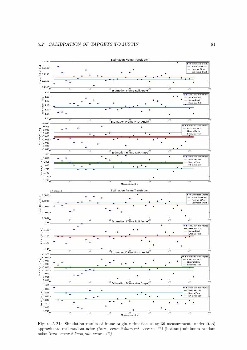
5.2. CALIBRATION OF TARGETS TO JUSTIN 81
Figure 5.21: Simulation results of frame origin estimation using 36 measurements under (top)approximate real random noise (tran. error-2.5mm,rot. error - 2◦) (bottom) minimum randomnoise (tran. error-2.5mm,rot. error - 2◦)

82 CHAPTER 5. POSE ESTIMATION BY USING THE IR TRACKING SYSTEM
For the real procedure on Justin we used 5 × 5 measurements to calibrate the hand andhead joints each. The hand calibration may be subject to errors independent of the trackingsystem, mainly the internal errors of the kinematic chain. We test the calibration of thetargets to the hand with different kinematic configurations of the arm. In Fig.5.22 threeexamples of these different configurations are shown. In Table 5.1 the deviations between10 estimated hand mounting frames T tcphaT are shown. We also compute the deviationsbetween 6 different estimated head mounting frames T hheT (Table 5.2). Since the internalerrors of the kinematic chain of the arm do not affect the head joint, we vary the positionof the torso either shorter or higher and we rotate it within the tracking systems volume.The deviations on the head joint are slightly higher than those of the arm, this is duemainly to the pan-tilt unit’s RoM. It is much more limited to that of the hand’s joint.
Figure 5.22: Three different kinematic configurations for Frame Estimation
Table 5.1: Hand Mounting Frame Deviations throughout 10 kinematic configurations
Metric t (cm) roll(◦) pitch(◦) yaw(◦)std 0.119 0.63 0.34 0.98
Table 5.2: Head Mounting Frame Deviations throughout 6 torso positions
Metric t (cm) roll(◦) pitch(◦) yaw(◦)std 0.31 0.623 0.579 1.22

5.3. ERROR IDENTIFICATION 83
5.3 Error IdentificationNow that the missing transformations (T hheT and T tcphaT ) of the implicit loop closure (Fig.5.4)are obtained from the calibration procedure, the pose of Justin’s TCP can be estimated.To recall the implicit loop closure, TCPfk and TCPart are both the pose of the TCP w.r.t.the head joint (T tcph ), however each of them are obtained with a different loop closure:
TCPart = T tcph = (T hart)−1(T tcpart ) = (T heTart ThheT )−1(T haTart T
tcphaT ) (5.45)
TCPfk = T tcph = T ahTtcpa (5.46)
TCPfk is the pose of the TCP computed using the measured joint positions with a forwardkinematic model (ie. this is the pose that Justin is reaching according to its position sensorson each joint). TCPart is the pose of the TCP estimated by the tracking system. IdeallyTCPart := TCPfk, however, as can be seen in Fig.5.23 this is not the case.
Figure 5.23: Measured TCPfk vs. Estimated TCPart
The error between TCPart and TCPfk can be represented as an error tuple e =< et, eθ >extracted from the ∆T = (TCPart)−1TCPfk as shown in Fig.5.24.
Figure 5.24: Error between TCPart and TCPfk: ∆T = (TCPart)−1TCPfk
The error tuple e is composed of et = (∆T (t)) which is the translational component of ∆Tthat represents the translational error between the coordinate frames. eθ = angleaxis(∆T (R))is the angle around the rotation axis of the rotational component of ∆T in angle-axis rep-resentation. When representing a rotation matrix R in angle-axis form we obtain a vectorv which is the direction of the rotation axis and an angle θ which is the rotation it.

84 CHAPTER 5. POSE ESTIMATION BY USING THE IR TRACKING SYSTEM
We generate 30 random poses and estimate the error e between TCPart and TCPfk.To evaluate the reliability of the tracking system we reproduce these same poses andestimations for different Justin positions within the tracking system volume. We set thetorso of Justin to 0◦,90◦ and −90◦ w.r.t. the ART base coordinate system as shown inFig.5.25.
Figure 5.25: Justin within ART camera setup
We test five positions listed in Table.5.3, we evaluate the translation component of theerror tuple et by comparing its length ||et|| throughout all the different poses and positions(Fig.5.26). In the real set-up only four cameras are functional (c1,c2,c4,c6), therefore movingJustin around will cause occlusion of the hand marker to some of the cameras. To estimatea robust 6DOF pose from the tracking targets at least two cameras need to have a fullview of the target. As can be seen, the errors of Position-4 are slightly higher than all ofthe other positions. This is due to the camera occlusions.

5.3. ERROR IDENTIFICATION 85
Table 5.3: Estimated errors with different Justin torso positions.
Position 1 2 3 4 5Torso Angle 0◦ 90◦ 90◦ −90◦ 90◦
max ||et|| (cm) 0.86 0.79 0.79 1.04 0.82mean ||et|| (cm) 0.62 0.56 0.56 0.76 0.48std ||et|| (cm) 0.1 0.11 0.11 0.12 0.15max ||eθ|| (◦) 1.34 1.86 1.86 1.59 1.23mean ||eθ|| (◦) 0.93 1.20 1.66 1.14 0.89std ||eθ|| (◦) 0.27 0.31 0.32 0.27 0.21
Figure 5.26: Estimated TCP translational errors

86 CHAPTER 5. POSE ESTIMATION BY USING THE IR TRACKING SYSTEM
Figure 5.27: Estimated TCP rotational errors
From our complete evaluation we are confident that this method can be used as a groundtruth for our proposed pose estimation method. However, some additional restrictions needto be taken care of in order for this method to work.
5.4 Method LimitationsAs presented earlier, the position of Justin with respect to the camera system can playa large role in the precision of the tracking system. The positions and kinematic config-urations of Justin need to be controlled and set to meet the specific requirements of thetracking system. Additionally, the mounting of the tracking targets needs to be verified bythe human-user, since the hand is in constant movement, after a certain time (dependingon how they are attached) the tracking targets can loosen up. After our thorough evalua-tion of this method we demonstrated that it is robust under the controlled environment.It could be used as an independent method to estimate the bounds of the error of the TCPend-pose with the restriction that it needs a calibration procedure every time it wants to beused. The aim of our work is to estimate the TCP errors with as less human interventionand restrictions as possible, therefore we only use this estimation method as a ground truthfor our own.

5.5. SUMMARY 87
5.5 SummaryIn this chapter we implemented a pose estimation method using the IR optical trackingsystem mounted in Justin’s lab. In order to use the tracking system, tracking targets needto be calibrated to find the pose of the joints where they are mounted on w.r.t. the trackingsystem base coordinate frame. A thorough description of the tracking target calibrationprocedure is presented. We evaluated our calibration procedure on synthetic and real data.With real data we achieved a standard deviation of 0.1mm on the translational componentof the hand joint and 0.3mm of the head joint form several calibration runs. The methodfor identifying the error between the measured TCP end-pose and the estimated TCPend-pose with the tracking system is presented. From the evaluation results, we concludedthat this method is robust and efficient under certain limitations. These limitations areregarding possible occlusions by the position of Justin within the lab. We will use thismethod as a ground truth to our pose estimation method by comparing their identifiederrors w.r.t. the measured TCP end-pose. This evaluation procedure was controlled to fitthe requirements of the tracking system.

Chapter 6
Pose Estimation by using 3DRegistration
The basic principle of estimating Justin’s TCP end-pose by using 3D registration is toregister (find the rigid motion) a point cloud of the hand in a random pose TCP to themodel of the hand with known pose TCPO (Fig.6.1).
Figure 6.1: (top-left) model of the hand with known TCPO end-pose (top-right) random pose ofthe hand with unknown TCP end-pose (bottom) Pose estimation with 3D registration principle:H is the rigid motion between the random pose and the model (TCP → TCPO)
88

89
If TCPO (the estimated origin of the model described in Chapter 4) is fixed to the modeland H is the rigid transformation of TCP → TCPO then H can be formulated as:
H = (TCP )−1TCPO (6.1)
We can compute the pose of TCP in the sensor coordinate system as follows:
TCP = T tcps = TCPO(H)−1 (6.2)
The implicit loop closure of Justin’s upper body kinematics enables us to relate our esti-mated pose TCPreg to the measured pose from forward kinematics TCPfk.
TCPreg = T hwTshT
tcps (6.3)
TCPfk = T hwTahT
tcpa (6.4)
Figure 6.2: Justin’s Implicit Loop Closure using the Stereo Vision System
We use Justin’s head as our reference coordinate system to close the sensory system kine-matic chain with the arm kinematic chain. We use Justin’s base as the world coordinatesystem. T hw is the transformation of the world coordinate system to the head joint, com-puted by simple forward kinematics. T sh is the transformation of the head joint to the

90 CHAPTER 6. POSE ESTIMATION BY USING 3D REGISTRATION
sensor origin, this is generated by the stereo calibration process. T ah is the transformationof the head to the arm base, computed by a simple forward kinematic model. T tcpa is thetransformation from arm base to tcp, computed by a forward kinematic model consideringthe measured torques and gear stiffness. The forward kinematics is computed as describedin Chapter 4.2.1. T tcps is the pose estimated by the rigid transformation between the ran-dom pose and the model (Eq.6.2) obtained from our 3D registration method. In Chapter 3we describe a two-step procedure for estimating the rigid motion between two point cloudsH (ie. TCP → TCPO). First, an initial guess for rigid motion (Hi) between a randompoint cloud P and the modelM is estimated. This guess yields a coarse registration, whichis then fine-tuned by applying ICP on all the points of both point clouds. We evaluatedtwo approaches for obtaining Hi:
1. Textured-based registration: An initial guess Hi is estimated by extracting the SIFTkeypoints of P and M and registering them with the ICP algortihm.
2. Surface/Combined-based registration: An initial guess Hi is estimated by findingcorrespondences with local descriptors based on surface (FPFH,SHOT) and com-bined surface/texture (CSHOT) information. We calculate the rigid transformationbetween the matched correspondences of P and M by using the Sample ConsensusInitial Alignment (SAC-IA) method.
An initial guess Hfk can also be computed by using the measured pose from forwardkinematic TCPfk. To compute Hfk, TCPfk is converted to sensor coordinates (TCPfks)as follows:
TCPfks = (T hwT sh)−1TCPfk (6.5)
Then Hfk is formulated as:Hfk = TCPO(TCPfks)−1 (6.6)
To improve the quality of the initial guess Hi (computed by the textured or surface-basedregistration approaches) we use Hfk as a pre-guess to the registration procedure. We alsotry using only Hfk as a direct initial guess. Therefore, we compare five methods for esti-mating H:
Hfk →
→ICP (p ∈ SIFT (P ),m ∈ SIFT (M))SACIA(fpfh(p) ∈ P, fpfh(m) ∈M)SACIA(shot(p) ∈ P, shot(m) ∈M)SACIA(cshot(p) ∈ P, cshot(m) ∈M)
→ Hi → ICP (p ∈ P,m ∈M)→ H
The first method is using Hfk as the direct initial guess. The second method is usingHfk as a pre-guess to an ICP registration between the SIFT keypoints of P and M . Thelast three use Hfk a pre-guess to a SAC-IA registration method using FPFH, SHOT andCSHOT descriptors. All of these methods yield to an initial registrationHi and are followedby a final step of applying an ICP algorithm over all the points in both P and M .

6.1. ERROR IDENTIFICATION 91
6.1 Error IdentificationTCPfk is the pose of the TCP computed using the measured joint positions with a forwardkinematic model. TCPreg is the pose of the TCP estimated by 3D registratiion. IdeallyTCPreg := TCPfk, however, as can be seen in Fig.6.3 (and demonstrated in Chapter 5)this is not the case.
Figure 6.3: Measured TCPfk vs. Estimated TCPreg
We used the same error representation as the one used for the ART estimated error(Described in Chapter 5.3 and Fig.5.24). Now the error tuple e =< et, eθ > is extractedfrom the ∆T = (TCPreg)−1TCPfk as shown in Fig.6.4.
Figure 6.4: Error between TCPreg and TCPfk: ∆T = (TCPreg)−1TCPfk

92 CHAPTER 6. POSE ESTIMATION BY USING 3D REGISTRATION
6.2 Error Evaluation MethodTo evaluate the identified errors using 3D registration we compare them to our error groundtruth. As described in Chapter 5 we generate this ground truth by estimating the TCP end-pose errors with an IR tracking system. Therefore, to apply a direct comparison betweenthe two estimated errors we estimate TCPreg and TCPfk in the ART world coordinatesystem. This generates a double loop closure as seen in Fig.6.5.
Figure 6.5: Justin’s Implicit Loop Closure for evaluation using the Stereo Vision System and ARTtracking system
We substitute T hw with T heTart ThheT in Eq.6.3 and Eq.6.4 and they are now expressed as
follows:TCPfk = T tcph = T heTart T
hheTT
ahT
tcpa (6.7)
TCPreg = T tcph = T heTart ThheTT
shT
tcps (6.8)

6.2. ERROR EVALUATION METHOD 93
The estimated pose obtained by the tracking system is estimated by:
TCPart = T tcph = (T heTart ThheT )−1(T haTart T
tcphaT ) (6.9)
Where T heTart and T haTart are the 6DOF measurements of the tracking targets. T hheT andT tcphaT are the transformation between tracking targets and joint origins obtained by thecalibration procedure described in Chapter 5.
Figure 6.6: Error between TCPreg and TCPfk: ∆Treg = (TCPreg)−1TCPfk and Error betweenTCPart and TCPfk: ∆Tart = (TCPart)−1TCPfk
Figure 6.7: Measured TCPfk vs. Estimated TCPreg vs. Estimated TCPart

94 CHAPTER 6. POSE ESTIMATION BY USING 3D REGISTRATION
6.3 Method Limitations
Our pose estimation method has limitations due to the arm kinematics (physical) andstereo vision system. The physical limitations concern Justin’s reach (max) and the closestconfiguration to the head without colliding (min) with its own body (Fig.6.8). We callthese the maximum and minimum physical limitations, where the maximum is 0.6m andthe minimum is 0.2m from the sensor origin in the z-direction.
Figure 6.8: Physical Limitations (left)minimum limit 0.2m from the sensor origin (right)maximumlimit 0.6m from the sensor origin
Our pair-wise registration methods rely on having a complete view of the hand. Pointclouds of the hand with cut-off portions (ie. missing/occluded fingers) will generate faultyregistrations. We cannot select any random pose because the FOV (32◦ × 20◦) of thestereo vision system is limited in the depth range between 0.2 and 0.6m. To verify this, wegenerated point clouds of the hand from the minimum to the maximum depth limitations,by setting the TCP end-pose in the line of sight of the sensor origin with a depth incrementof 2cm (Fig.6.9).
Figure 6.9: Point clouds of the hand with the TCP end-pose at the line of sight from min to maxphysical depth limits. (left) frontal view (right) side view

6.3. METHOD LIMITATIONS 95
We estimate the pose of this set of point clouds with the five pair-wise registration methodsand with the ART tracking system method. As can be seen in Fig.6.10, the translationalerrors ||et|| with 3D registration methods based on local descriptors between depth valuesof 0.2-0.32m are quite unstable. This is due to the cut-off point clouds generated in thesedepth values (Fig.6.11).
Figure 6.10: Estimated TCP translational errors (top) between min-max physical limitations(bottom) between min-max stability limitations
Figure 6.11: (left) cut-off point cloud (right) faulty registration to model

96 CHAPTER 6. POSE ESTIMATION BY USING 3D REGISTRATION
After 0.55m the errors increase due to the variable depth resolution of the point clouds.Therefore, we choose the depth values between 0.32-0.55m as the stability range of the poseestimation method based on 3D registration. Within the stability range it can be seen thatthe estimated errors with 3D registration exhibit a similar behavior as the ground trutherrors (estimated by ART method). The ART method estimates a max error of 1.03 cmand mean error of 0.89 cm. The errors estimated by 3d registration methods are almostidentical, they show a max error of around 1.12 cm and mean error of 0.98 cm.
Table 6.1: Estimated translational errors with increasing depth values.
Method ART fk-ICP SIFT FPFH SHOT CSHOTmax ||et|| (cm) 1.03 1.13 1.12 1.12 1.12 1.12mean ||et|| (cm) 0.89 0.99 0.98 0.97 0.97 0.97std ||et|| (cm) 0.11 0.17 0.16 0.17 0.17 0.17
These results were generated from a restricted set of kinematic configurations. Since theTCP end-pose only varies in z-direction of the sensor origin, the joint positions w.r.t. eachother are very similar. We want to identify errors with diverse kinematic configurations,this way all of the joints will have a contribution to the TCP error. Therefore, consideringthe FOV and the stability range we create a verification volume (Fig.6.12).
Figure 6.12: Verification Volume (a/d are the min/max physical limits of Justin’s arm kinematicchain and b/c are the min/max limits of the 3D registration method)

6.4. RANDOM POSE GENERATOR 97
6.4 Random Pose Generator
To obtain different kinematic configurations of the arm we generate random poses withinthe identified verification volume. The random pose generation procedure consists of thefollowing steps (Fig.6.13):
1. Find a random Z-value within the stability range of the 3D registration method(Zmin = 0.32cm,Zmax = 0.55cm).
2. Find a random X-value depending on the previously obtained Z-value. The left andright X-limits (xl,xr) can be expressed based on the Z-value as follows:
xl = −(Z tan(FOVh/2)− w/2) (6.10)
xr = Z tan(FOVh/2)− w/2 (6.11)
Where FOVh is the horizontal angle of the Field-Of-View of the stereo vision systemand w is the hand width. We randomly choose an x value within xl and xr and thenrandomly choose if we use xr or xl by generating a random number rx = rand(0, 1)and using the following equation:
X ={rand(xl) rx < 0.5rand(xr) rx > 0.5 (6.12)
3. To find a random Y -value we express the top and bottom Y -limits (yt,yb) in Z-valuesas follows:
yt = −(Z tan(FOVv/2)− (h− offsett)) (6.13)
yb = Z tan(FOVv/2)− (offsetb) (6.14)
Where FOVv is the vertical angle of the Field-Of-View of the stereo vision system,h is the hand height and offsetb and offsett are the top and bottom offsets of thehand height w.r.t. the line of sight. We randomly choose a y value within yt and ybusing the same procedure applied to X, we generate ry = rand(0, 1), then:
Y ={rand(yt) ry < 0.5rand(yb) ry > 0.5 (6.15)
4. We set the models origin TCPO to the random position w.r.t. the sensor coordinatesystem with the random X,Y, Z values obtained in the previous steps.
5. The final step is to rotate the new TCPO around it’s Z-axis with a random anglebetween the range of angles used to generate the model (φmin and φmax), the randomTCP is formulated as:
TCPrand = TCPO(X,Y, Z)Rotz(θz(rand(φmax − φmin))) (6.16)

98 CHAPTER 6. POSE ESTIMATION BY USING 3D REGISTRATION
Figure 6.13: Random TCP end-pose generation.
The generated random pose TCPrand is then loaded to an inverse kinematics solver inOpenRave1. The solver we use is the ikfast module which solves for closed-form solutionsto compute the joint angles of the arm for a desired pose. An example of different TCPrandand their kinematic configurations obtained by inverse kinematics can be seen in Fig.6.14.
Figure 6.14: Random TCP end-poses within the Verification Volume (notice the different kine-matic configurations)
1OpenRave or Open Robotics Automation Virtual Environment is an environment for testing,developing, and deploying motion planning algorithms in real-world robotics applications. Weuse this environment to run all of the interactions with Justin. For further reference, refer to:http://openrave.org/en/main/index.html

6.5. EXPERIMENTAL RESULTS 99
6.5 Experimental ResultsTo evaluate the performance of the pose estimation methods we create 5 different testenvironments. Two variables are changed to create these environments: (i) the exposuretime of the cameras and (ii) the background (Table 6.2). By varying the exposure time,we simulate a darker or brighter environment. The higher the exposure time the brighterthe images of the stereo vision system. The background is changed by rotating Justin’storso within the lab. As it can be seen in Fig.6.15, a torso rotation of 90◦ generates anenvironment with a cluttered background and rotations 0◦ and −90◦ have semi-clutteredbackground.
Table 6.2: Testing Environments for Error Identification.
Environment 1 2 3 4 5Torso Rotation 0◦ 90◦ 90◦ −90◦ 90◦Exp. Time (ms) 30 30 15 20 30Background Semi-Cluttered Cluttered Cluttered Semi-Cluttered Cluttered
Figure 6.15: Different Environments for Error Identification Testing using 3D Registration andART methods

100 CHAPTER 6. POSE ESTIMATION BY USING 3D REGISTRATION
For the first environment 28 random poses are generated. The translational errors ||et||estimated from the ART and all the registration methods are shown in Fig.6.16.
Figure 6.16: Estimated translational errors ||et|| for Environment-1
It can be seen that even though the random poses were generated within the verificationvolume, some faulty registrations are still obtained. The extremely erroneous registrations(ie. Pose index 4, 9 and 22) are generated from the local descriptor based methods (FPFH,SHOT, CSHOT). In Chapter 4 these methods exhibited robust and stable behavior, how-ever in that chapter the point clouds of the hands were completely segmented and themotion between them was structured (ie. 10◦ steps). In this case, the same pre-processingfilters are applied to the point clouds and the cut-off point clouds are no longer generated,however since we are generating random poses of the kinematic chain, parts of the arm canbe captured in the point clouds.

6.5. EXPERIMENTAL RESULTS 101
The previously described behavior can be seen in Fig.6.17. The generated point cloud isnoisy (notice the finger areas) and contains surface information of the last link of the arm’skinematic chain. Even though the Hfk is used as a pre-guess for the initial guess estima-tion, the local descriptor based methods (FPFH,SHOT,CSHOT) seem to be suboptimal inthese scenarios. This is mainly due to the SAC-IA estimation method not the descriptorsthemselves. SAC-IA is based on choosing a random match between a descriptor from therandom point cloud P to a list of 10 corresponding descriptors in the model point cloudM (Chapter 3). When registering noisy point clouds these random matches can lead to afaulty rigid transformation.
Figure 6.17: Pose index 22: (left) Generated point cloud (right) Faulty registration to model
It must be noted that the SIFT and fk-ICP based methods do not exhibit these faultyregistrations. This is because they are only based on point-to-point correspondences inthe 3D space and since the pre-guess Hfk is used the point clouds are already close to themodel. Therefore, the final ICP step correctly merges the points of the random point cloudP nearest to the model M . However, they still generate some above average translationalerrors. For example, if we compare the ||et|| estimated for pose index 11 (in Fig.6.16)and the one estimated for pose index 17, it is more than twice the error value. If wevisually compare these two registrations (Fig.6.18), the registration of the point cloud ofpose index 11 yields to a shifty registration compared to that of pose index 17 which is agood registration.
Figure 6.18: (left) Shifty Registration of pose index 11 (right) Good registration of pose index 17

102 CHAPTER 6. POSE ESTIMATION BY USING 3D REGISTRATION
We identified that the peak translational errors ||et|| are generated from faulty and shiftyregistrations. In order to deal with them we evaluate the fitness score2 of the registrations.In Fig.6.19 a plot of the fitness scores corresponding to the registrations obtained from thepoint clouds of Environment-1 is shown. We identified that the worst fitness scores (peaks)correspond directly to the shifty and faulty registrations.
Figure 6.19: Fitness scores of 3D registration methods for Environment-1
To reject the shifty and faulty registrations without any visual intervention we applya RANSAC [42] outlier rejection algorithm on the fitness scores of the complete set ofrandom poses. Therefore, the estimated translational ||et|| and rotational errors eθ willbe computed from only good registrations. By applying this rejection we can compare therobustness of the different registration methods by identifying how many registrations arerejected by each.
2The fitness score of a pair-wise registration is the sum of squared Euclidean distances between thenearest corresponding points of both point clouds.

6.5. EXPERIMENTAL RESULTS 103
6.5.1 Environment-1
28 random poses are generated. The faulty and shifty registrations are rejected usingRANSAC on their fitness scores. Overall the registration methods reject the same numberof poses and have identical mean fitness scores (Table 6.3,Fig.6.21). The maximum ||et|| isestimated to be around 0.85 cm for all methods including the ART method (Fig.6.20) andthe maximum eθ is around 2◦. For this environment no registration method out-performsthe others and they are all consistent with the estimated errors from the ART method.
Table 6.3: Estimated errors in Environment-1
Method ART fk-ICP SIFT FPFH SHOT CSHOTmax ||et|| (cm) 0.86 0.85 0.85 0.85 0.85 0.84mean ||et|| (cm) 0.62 0.65 0.65 0.65 0.69 0.68std ||et|| (cm) 0.1 0.13 0.13 0.12 0.1 0.11max eθ (◦) 1.48 2.3 2.07 2.3 2.06 2.06mean eθ (◦) 0.94 0.85 0.83 0.84 0.88 0.8std eθ (◦) 0.29 0.56 0.54 0.56 0.56 0.52
mean fit.score (µm) - 2.63 2.63 2.63 2.63 2.63rejected poses - 9 9 9 9 9
Figure 6.20: Translational errors ||et|| of 3D registration methods for Environment-1

104 CHAPTER 6. POSE ESTIMATION BY USING 3D REGISTRATION
Figure 6.21: Evaluation of 3D registration methods for Environment-1: (top) Rotational errors eθ(bottom) Fitness scores

6.5. EXPERIMENTAL RESULTS 105
6.5.2 Environment-2
This environment has the same illumination setup as environment 1, but with a clutteredbackground. From the 30 generated random poses, 10 registrations were rejected (with theFPFH rejecting 11) (Table 6.4,Fig.6.23). The estimated maximum ||et|| is of around 0.98cm for the registration methods, it is around 2mm higher than the ground truth (Fig.6.22).The point-to-point correspondence based methods (fk-ICP, SIFT) exhibit a slightly highermaximum eθ compared to the other registration methods. Overall the behavior of theregistration methods is consistent with that of environment 1.
Table 6.4: Estimated errors in Environment-2
Method ART fk-ICP SIFT FPFH SHOT CSHOTmax ||et|| (cm) 0.79 0.98 0.98 0.98 0.98 0.99mean ||et|| (cm) 0.56 0.69 0.70 0.70 0.72 0.72std ||et|| (cm) 0.11 0.13 0.12 0.13 0.11 0.12max eθ (◦) 1.86 2.93 2.93 1.76 1.75 1.75mean eθ (◦) 1.2 0.80 0.74 0.70 0.68 0.68std eθ (◦) 0.31 0.69 0.64 0.51 050 0.51
mean fit.score (µm) - 1.9 1.9 1.84 1.9 1.9rejected poses - 10 10 11 10 10
Figure 6.22: Translational errors ||et|| of 3D registration methods for Environment-2

106 CHAPTER 6. POSE ESTIMATION BY USING 3D REGISTRATION
Figure 6.23: Evaluation of 3D registration methods for Environment-2: (top) Rotational errors eθ(bottom) Fitness scores

6.5. EXPERIMENTAL RESULTS 107
6.5.3 Environment-3
This environment has the same background as Env-2, but with a darker illumination setup.The estimated et and eθ are the same values as for Env-2 (Table 6.5,Fig.6.24,Fig.6.25). Thiswas expected since we only changed the camera parameters. From the 30 random poses fk-ICP, SIFT and FPFH methods rejected 10 registrations, however the SHOT-based methodsrejected 14. This means that these descriptors are more susceptible to illumination changes,mainly if the illumination changes the stereo processing changes as well, which can possiblygenerate noisier data.
Table 6.5: Estimated errors in Environment-3
Method ART fk-ICP SIFT FPFH SHOT CSHOTmax ||et|| (cm) 0.79 0.97 0.97 0.97 0.97 0.97mean ||et|| (cm) 0.56 0.67 0.69 0.68 0.71 0.70std ||et|| (cm) 0.11 0.14 0.14 0.15 0.14 0.14max eθ (◦) 1.86 1.92 1.88 1.92 1.07 1.25mean eθ (◦) 1.2 0.81 0.68 0.78 0.49 0.52std eθ (◦) 0.31 0.63 0.52 0.58 0.35 0.37
mean fit.score (µm) - 1.84 1.84 1.89 2.07 2.07rejected poses - 10 10 10 14 14
Figure 6.24: Translational errors ||et|| of 3D registration methods for Environment-3

108 CHAPTER 6. POSE ESTIMATION BY USING 3D REGISTRATION
Figure 6.25: Evaluation of 3D registration methods for Environment-3: (top) Rotational errors eθ(bottom) Fitness scores

6.5. EXPERIMENTAL RESULTS 109
6.5.4 Environment-4
For this environment, we use a different semi-cluttered background with semi-bright illu-mination. The max ||et|| detected from the registration methods and the ART methodare higher than the previous tests, but are consistent with each other (Table 6.6,Fig.6.26).Overall no registration method outperforms another, they all reject 12 registrations from30 (expect FPFH with 11 rejections) and estimate the same rotational errors eθ and showalmost identical fitness scores (Fig.6.27).
Table 6.6: Estimated errors in Environment-4
Method ART fk-ICP SIFT FPFH SHOT CSHOTmax ||et|| (cm) 1.04 1.07 1.06 1.06 1.07 1.06mean ||et|| (cm) 0.76 0.69 0.71 0.70 0.73 0.73std ||et|| (cm) 0.12 0.18 0.17 0.19 0.19 0.16max eθ (◦) 1.59 1.84 1.79 1.84 1.78 1.77mean eθ (◦) 1.14 0.77 0.64 0.78 0.62 0.64std eθ (◦) 0.27 0.64 0.55 0.64 0.56 0.55
mean fit.score (µm) - 2.22 2.22 2.22 2.21 2.16rejected poses - 12 12 12 11 12
Figure 6.26: Translational errors ||et|| of 3D registration methods for Environment-4

110 CHAPTER 6. POSE ESTIMATION BY USING 3D REGISTRATION
Figure 6.27: Evaluation of 3D registration methods for Environment-4: (top) Rotational errors eθ(bottom) Fitness scores

6.5. EXPERIMENTAL RESULTS 111
6.5.5 Environment-5
This environment is identical to Env-1. As it can be seen in Table 6.7 from the 30 randomposes 15 registrations were rejected from the fk-ICP, SIFT and FPFH methods and 18 forthe SHOT-based methods. Rejecting more than half of the total number of poses affectsthe error identification. All of the registration methods yield the same max ||et|| as theART method except for the SHOT methods, however the mean ||et|| are around the samevalues.
Table 6.7: Estimated errors in Environment-5
Method ART fk-ICP SIFT FPFH SHOT CSHOTmax ||et|| (cm) 0.82 0.81 0.82 0.82 0.52 0.52mean ||et|| (cm) 0.48 0.48 0.49 0.48 0.42 0.42std ||et|| (cm) 0.15 0.17 0.17 0.17 0.07 0.08max eθ (◦) 1.23 1.39 1.19 1.36 1.01 1.01mean eθ (◦) 0.89 0.63 0.52 0.67 0.40 0.41std eθ (◦) 0.21 0.49 0.43 0.46 0.33 0.33
mean fit.score (µm) - 1.85 1.85 1.85 1.9 1.9rejected poses - 15 15 15 18 18
Figure 6.28: Translational errors ||et|| of 3D registration methods for Environment-5

112 CHAPTER 6. POSE ESTIMATION BY USING 3D REGISTRATION
Figure 6.29: Evaluation of 3D registration methods for Environment-5: (top) Rotational errors eθ(bottom) Fitness scores

6.5. EXPERIMENTAL RESULTS 113
6.5.6 Overall Performance
After evaluating the five test environments individually we realize that identifying the TCPend-pose error by using 3D registration is feasible. However, every method exhibited somedraw-backs. For example, the point-to-point based correspondence methods (fk-ICP,SIFT)showed sometimes higher rotational errors eθ but the translational errors ||et|| were alwaysconsistent. The SHOT-based methods had higher registration rejections than the othermethods, in environment 5 they rejected more than half of the random poses yieldingto an incomplete error analysis. To further evaluate the performance of all registrationmethods we compute the average computation time from all the random poses of the 5environments (150 poses). These computation times are based on registrations of pointclouds downsampled with a 2mm voxel leaf size. The random point clouds P have anaverage of 20k points and the downsampled model M has a total number of 65k points.We also evaluate the performance based on how many rejections each method generates,this is calculated as a success rate which is formulated as follows:
SuccessRate(%) = Nt −RtNt
× 100 (6.17)
Where Nt is the total number of poses and Rt is the total number of rejected poses fromfaulty registrations (applying RANSAC on the fitness scores).
Table 6.8: Overall Performance of Pose Estimation by using 3D Registration
Method fk-ICP SIFT FPFH SHOT CSHOTMean Comp. Time (s) 64 170 329 731 512
Succes Rate (%) 62.42 62.42 61.74 58.39 57.72
As can be seen, the point-to-point based correspondence methods (fk-ICP,SIFT) are muchfaster than the methods based on local descriptor matching (FPFH,SHOT,CSHOT). Thisis due to the dimensionality of the search spaces in each method. The higher the searchspace, the longer it will take to find correspondences. Based on the individual environmenttests the FPFH-based method is the most stable and consistent in both the rotational eθand translational errors ||et||, however it’s computation time is not optimal. The SHOT-based methods have a lower success rate and the highest computation time, however theestimated errors exhibit the same consistency as the FPFH-based method (when not re-jecting too many registrations). It is possible that due to the high dimensionality of thesedescriptors (SHOT-358/CSHOT-1344) the SAC-IA method for finding correspondences be-haves inefficiently, causing this excess of registration rejections. Therefore, if consistencyin the rotational error eθ is of high importance and fast computation time is not a require-ment, then the local descriptor-based registration methods should be used. However, iffast computation time is necessary then the fk-ICP or SIFT-based registration methodsare best suited.

114 CHAPTER 6. POSE ESTIMATION BY USING 3D REGISTRATION
6.6 SummaryIn this chapter we describe our proposed pose estimation method by using 3D registrationtechniques.The estimated pose is used to identify the errors in the TCP end-pose. Theseerrors are estimated with five different registration methods. These methods are evaluatedby comparing their estimated errors with the errors estimated by using the IR ART trackingsystem. For the registration methods to work, the pose estimation setup needs to comply tocertain limitations. These limitations consist of physical limitations of Justin’s kinematicsand of the stereo vision system. We deal with these limitations by creating a verificationvolume. A random pose generator that satisfies the verification volume was implemented.Point clouds of these poses are created and then registered to a model. To reject faulty orshifty registrations a RANSAC-based outlier rejection algorithm is applied to the fitnessscores of the set of registrations from random poses. This procedure was evaluated in fivedifferent environments. The estimated errors by using 3D registration are consistent withthe errors estimated from the ART-based methods.

Chapter 7
Application: Bound-Identificationof Justin’s TCP Errors
The application of this thesis was to create a verification routine to identify the errorbounds (ie. max ||et|| and eθ) of the TCP end-pose. In the previous chapter, the feasibilityof identifying these errors using 3D registration techniques was evaluated.
As an offline initial step for this routine, a model of the hand has to be generated. Theprocedure for the model generation is thoroughly described in Chapter 4. It is only neces-sary to generate new models of the hand when the calibration of the stereo vision systemis modified.
The routine consists of the following steps:
1. N-TCP poses are created by the random pose generator (Chapter 6.4).
2. For each random pose n ∈ N an individual error identification pipeline is executed,where the output is an error tuple ek =< et, eθ > and a fitness score fk representingthe quality of the registration (Chapter 6.1).
3. Once the complete set of error tuples E = (e1, · · · , ek, · · · , eN ) and fitness scores F =(f1, · · · , fk, · · · , fN ) are estimated, a RANSAC outlier rejection algorithm is appliedto the fitness scores. A subset of error tuples E∗ corresponding to the remainingsub-set fitness scores F ∗ = RANSAC(F ) is created.
4. The maximum bounds eb of the TCP end-pose error are calculated as:
eb =< max(||et|| ∈ E∗),max(eθ ∈ E∗) > (7.1)
Which is the maximum length of the translational error et in subset E∗ and the maximumrotational error eθ. In Fig.7.1 an outline of our verification routine is depicted.
115

116CHAPTER 7. APPLICATION: BOUND-IDENTIFICATION OF JUSTIN’S TCP ERRORS
Figure 7.1: Verification Routine
The Point Cloud Processing stage is addressed in Chapter 2. A raw point cloud of thehand has around 100k points, the acquisition of this point cloud takes around 5 seconds.Applying a voxel grid filter of 2mm leaf size and a statistical outlier removal filter takesaround 20 seconds. Therefore, the Point Cloud Processing stage takes around 25 seconds.The total computation time of each individual error identification pipeline is highly de-pendent on the registration method used for the Pose Estimation stage. In Chapter 6we computed the average computation times for the five different registration methods,however we did not address the feature estimation computation time. For the fk-ICPmethod features are not computed. In the SIFT-based method, the computation of theSIFT-Keypoints is included in the total registration time.

117
Therefore for these two methods the total computation time of an individual Error Iden-tification Pipeline is depicted in Table 7.1.
Table 7.1: Error Identification Pipeline Computation Time
Computation Time fk-ICP SIFTPoint Cloud Processing (s) 25 25Mean Pose Estimation (s) 64 170
Total (s) 89 155
For the local descriptor based methods (FPFH/SHOT/CSHOT), two steps are required:(i) surface normal estimation and (ii) descriptor estimation based on the surface normals. InPCL1 implementation of surface normal estimation and FPFH/SHOT/CSHOT descriptorestimation which use multi-core/multi-threaded paradigms using OpenMP are available.The total computation times of an individual Error Identification Pipeline using theseregistration methods are shown in Table 7.2. We compare the computation times whenusing 1,4 and 8 cores.
Table 7.2: Error Identification Pipeline Computation Time
Computation Times FPFH SHOT CSHOTCores 1/4/8 1/4/8 1/4/8
Point Cloud Processing (s) 25 25 25Normal Estimation (s) 2/1/1 2/1/1 2/1/1
Descriptor Estimation (s) 38/16/12 204/68/26 216/57/27Mean Registration Time (s) 329 731 512
Total (s) 394/371/367 962/825/783 755/595/565
As discussed in Chapter 6 these registration methods are sub-optimal regarding compu-tation time. For a total estimate of how long one run of a verification routine can take weconsider the fastest registration method (fk-ICP). The first step of the procedure is gen-erating the random poses with their joint angles calculated from inverse kinematics. Theikfast module in OpenRave takes around 10 ms per pose, so for 30 random poses the com-putation time is negligible. The total computation time of the Verification Loop dependson the number of cores available to compute individual Error Identification Pipelines. Ifonly one core in the processor is available, then the verification loop will be executed in asequential manner, as depicted in Fig.7.2. For 30 random poses using a sequential verifica-tion loop the total computation time is around 45 minutes. However, if more n-cores areavailable the total computation time is n-times faster. Therefore, if the verification loop isexecuted in a parallel manner (Fig.7.3) with 5 cores, the total computation time is around9 minutes.
1Open Source Point Cloud Library. http://www.pointclouds.org/

118CHAPTER 7. APPLICATION: BOUND-IDENTIFICATION OF JUSTIN’S TCP ERRORS
Figure 7.2: Sequential Error Identification
Figure 7.3: Parallel Error Identification

Chapter 8
Conclusions
Nowadays the trend in robotic applications is the interaction with unknown environmentsand the cooperation between robots and humans. For these robots to interact with hu-mans, achieve human-like mobility and compliant interaction, they require a light-weightdesign and flexibility in the joints of the kinematic chain. The light-weight design enablesmobility and ensures the safety of humans at the cost of low positioning accuracy. Thislow position accuracy is caused by the mechanical flexibilities in the joints and links, aswell as bending effects in the light-weight structures. This produces positioning errors atthe TCP end-pose of the kinematic chain. These errors are not trivial and affect the path-planning and grasping algorithms for object manipulation. In order to benefit from thelight-weight robot design it is crucial to identify the worst-case errors in the TCP end-pose,so they can be considered for manipulation tasks. Additionally, these errors need to beidentified with on-board sensors to avoid any human intervention or external sensing device.
This thesis proposed a verification routine using the on-board stereo vision system to com-pute the bounds of DLR’s Justin TCP end-pose errors. The routine is based on estimatingthe TCP end-pose by registering 3D point clouds of the hand created from the stereo visionsystem. It was fully implemented on Justin using the Open Source Point Cloud Libraryfor the point cloud processing and registration algorithms.
The first part of this thesis covers the 3D registration problem. Specifically, in Chapter2 we described the point cloud acquisition process from two stereo images to a 3D pointcloud. After creating the point clouds, we processed them with different filters in orderto reduce noise and computation time. This process takes from 25 to 30 seconds. Inmany applications, stereo vision is not preferred due to its variable depth resolution. Ourapplication is based on identifying the hand in the close range of the FOV of the cam-eras. In Chapter 6 we evaluated the effects of different depth values on 3D registration,we also changed the illumination settings and background to test if the registration tech-niques based on stereo data were consistent and we identified that with darker illuminationsettings the point clouds were noisier and could generate complications to some of the reg-istration techniques. In Chapter 3 we reviewed four different 3D registration methods. Thefirst method is based on registering keypoints extracted from intensity values of the point
119

120 CHAPTER 8. CONCLUSIONS
clouds using the SIFT algorithm. The other methods rely on a random sample consensusmatching approach using local feature descriptors (FPFH,SHOT,CSHOT). These meth-ods were then used in Chapter 4 to create partial models of the hand. In this chapter wepropose a partial model creation method called extended metaview registration. Since thehand is a self-occluding object we could not create a model by simply applying incrementalpair-wise registrations and loop-closure methods. We needed to reject some of the views, soin this method we avoid possibly faulty registrations by rejecting point clouds of the handbased on a descriptive statistical analysis of the minimum and maximum depth values. Wegenerate an inner and outer model and evaluate them by applying visibility consistencymeasures with synthetic models. After a thorough evaluation, we conclude that the pointclouds used to generate the outer model are noisier than the ones used to generate theinner model. The outer surface of the hand consists of transparent non-lambertian mate-rial, which causes difficulties for any stereo processing algorithm. Therefore, we use thegenerated inner model to estimate the pose of a random point cloud of the hand.
The second part of the thesis presents two pose estimation methods for the identificationof errors in Justin’s TCP end-pose. In Chapter 5 we described the pose estimation by us-ing the ART IR Tracking System. This method relies on a calibrated tracking system andtracking targets. These targets are mounted to Justin and we implemented a procedureto calibrate the mounted targets to the kinematic chain. This pose estimation methodis highly accurate and robust, however it relies on human intervention and external sens-ing devices, therefore we used it as the ground truth to our pose estimation method (byusing 3D registration), which is addressed in Chapter 6. In this chapter, we tackled thelimitations of the registration techniques in order to achieve estimated errors as consistentas the ground truth. We used the measured TCP end-pose from forward kinematics as apre-guess to the registration methods and we compared their estimated errors with a directICP registration using the measured pose as an initial guess. We tested these methods infive different scenarios. In two scenarios the difference in translational error between theregistration methods and the ground truth was of 2mm, in the other scenarios the differencewas negligible. The five registration methods yield almost identical estimated translationalerrors. The local descriptor based registration methods estimate more consistent rotationalerrors, however their computation time is sub-optimal.
The maximum translational error identified in the TCP end pose lies between 0.8− 1cmand the maximum rotational error was identified to be around 1 − 2◦. Even though theestimated errors were consistent with the ground truth, these were achieved with an approx-imate 60% success rate. To increase this success rate and achieve a more robust estimationeither the registration methods need to be improved (by surveying further local based reg-istration methods or exploring global registration method) or the point cloud processingneed to be improved in order to generate point clouds of the hands completely free of noiseand other surfaces.

121
In Chapter 7 an overview of the verification procedure is presented. Where we showedthat the verification routine can take from 45 minutes to 9 or less minutes depending on theavailable cores in the processor. Even though our proposed method has some limitationsit manages to generate consistent error identifications without any human intervention orexternal sensing device. This shows that using 3D registration techniques for identifyingthe position of the hand is feasible. The only system requirements for this procedure towork are a 3D sensing device and a robot arm with an end-effector (hand), thus the pro-posed error identification technique based on 3D registration can be implemented on anyhumanoid robot. Furthermore, this work can be extended to an online-verification loop .
Additionally, a further analysis of the estimated errors can be performed. By computingthe body Jacobian of an error vector and analyzing its coefficients, we can identify the jointthat has the most impact on that specific pose. This analysis can be applied throughoutall the generated error vectors. An optimization problem can be formulated to find acorrelation between Jacobians and error vectors. From this correlation, a hypothesis ofwhich joint or joints are consistently affecting the Cartesian end-pose can be generated.

Appendix A
Brief description of algorithms
A.1 Kd-tree for nearest neighbor searchThe computation of nearest neighbors is a fundamental step when processing 3D pointclouds. It is used to find correspondences, to find a set of local neighbors around a pointor to compute point features such as surface normal vectors of local surface descriptors [25].
A kd-tree (k-dimensional tree) is a space partitioning data structure that stores a set ofk-dimensional points in a tree structure. It is a binary search tree and it enables efficientrange and nearest neighbor searches. For a detailed description of this multi-dimensionalbinary search tree, refer to [83]. A detailed implementation of the kd-tree data structureadapted for n-dimensional spaces where n > 2 is present is the Open Source Point CloudLibrary [6]. The kd-tree of a set of 3D points is used as an input data structure for anearest neighbor search algorithm.
One of the most efficient nearest neighbor search methods is the approximate near-est neighbor search using FLANN (Fast Library for Approximate Nearest Neighbors)1.FLANN is a library for performing fast approximate nearest neighbor searches in highdimensional spaces. It contains a collection of algorithms found to work best for nearestneighbor search and a system for automatically choosing the best algorithm and optimumparameters depending on the dataset [84]. This library is integrated with the kd-treedatastructures of PCL to compute the nearest neighbors of a point.
1FLANN - Fast Library for Approximate Nearest Neigbors http://www.cs.ubc.ca/ mar-iusm/index.php/FLANN/FLANN [84]
122

A.2. SIFT (SCALE INVARIANT FEATURE TRANSFORMS) ALGORITHM 123
A.2 SIFT (Scale Invariant Feature Transforms) AlgorithmThe SIFT approach is an algorithm for image feature generation that takes an image andtransforms it into a large collection of local feature vectors2. Each of these feature vectors isinvariant to any scaling, rotation or translation of the image. The SIFT algorithm appliesa 4 step approach:
1. Scale-Space Extrema Detection:In this step locations and scales that are identifiable from different views of the sameobject are extracted. This is efficiently achieved using a scale space function. Thescale space is defined by a Gaussian function:
L(x, y, σ) = G(x, y, σ)∗I(x, y) (A.1)
Where ∗ is the convolution operator, G(x, y, σ) is a variable-scale Gaussian and I(x, y)is the input image. A Difference of Gaussians (DoG) technique is used to detect stablekeypoint locations in the scale-space. The scale-space extrema D(x, y, σ) is locatedby computing the difference between two images, one with scale k-times the other.Therefore, D(x, y, σ) is given by:
D(x, y, σ) = L(x, y, kσ)− L(x, y, σ) (A.2)
To detect the local maxima and minima of D(x, y, σ) each point is compared withits 8 neighbors at the same scale, and its 9 neighbors up and down one scale. If thisvalue is the minimum or maximum of all these points then it is an extrema.
2. Keypoint Localization:In this step, points from the list of extracted keypoints are eliminated. This is doneby finding keypoints that have low contrast or are poorly localized on an edge. Thisis achieved by calculating the Laplacian value for each keypoint found in the firststep. The location of extremum z is given by:
z = −δ2D
δx2
−1δD
δx(A.3)
If the function value at z is below a threshold value then this keypoint is excluded.This removes extrema with low contrast. To eliminate extrema based on poor local-ization it is noted that in these cases there is a large principle curvature across theedge but a small curvature in the perpendicular direction in the difference of Gaus-sian function. If this difference is below the ratio of largest to smallest eigenvector,from the 2x2 Hessian matrix at the location and scale of the keypoint, the keypointis rejected.
3. Orientation Assignment:In this step a consistent orientation is assigned to the keypoints based on local imageproperties. The keypoint descriptor can then be represented relative to this orienta-tion, achieving invariance to rotation.
2From "Object Recognition from Local Scale-Invariant Features", David G. Lowe [48]

124 APPENDIX A. BRIEF DESCRIPTION OF ALGORITHMS
The approach taken to find an orientation is:
• The scale of the keypoints is used to select the Gaussian smoothed image L fromstep 1.• The gradient magnitude m is computed as follows:
m(x, y) =√L(x+ 1, y)− L(x− 1, y)2 + (L(x, y + 1)− L(x, y − 1))2 (A.4)
• The orientation θ is computed as follows:
θ(x, y) = tan−1((L(x, y + 1)− L(x, y − 1))/(L(x+ 1, y)− L(x− 1, y))) (A.5)
• An orientation histogram is formed from the gradient orientations of samplepoints.• The highest peak of the histogram is located. This peak and any peak within80% of the height of this peak is used to create the keypoint with that orienta-tion.
In the case of multiple peaks from the last step, each peak is used for computing anew image descriptor for the corresponding orientation estimate. When computingthe orientation histogram, the increments are weighted by the gradient magnitudeand also weighted by a Gaussian window function centered at the interest pointand with its size proportional to the detection scale. To increase the accuracy of theorientation estimate, a rather dense sampling of the orientations is used, with 36 binsin the histogram. Moreover, the position of the peak is localized by local parabolicinterpolation around the maximum point in the histogram.
4. Keypoint Descriptor:Given the scale m(x, y) and orientation θ(x, y) estimate from the last step for eachkeypoint, a rectangular grid is laid out in the image domain, centered at the interestpoint, with its orientation determined by the main peak(s) in the histogram and withthe spacing proportional to the detection scale of the interest point. To give strongerweights to gradient orientations near the interest point, the entries in the histogramare also weighed by a Gaussian window function centered at the interest point andwith its size proportional to the detection scale of the interest point. Taken together,the local histograms computed at all the 4x4 grid points and with 8 quantized direc-tions lead to an image descriptor with 4x4x8=128 dimensions for each interest point.This resulting image descriptor is referred to as the SIFT descriptor.
The resulting SIFT keypoint descriptors are used to find correspondences between im-ages using a nearest-neighbor approach. For a more detailed description of the completealgorithm and matching stage refer to David Lowe’s publications [35] [48].

A.3. PRINCIPAL COMPONENT ANALYSIS 125
A.3 Principal Component AnalysisPrincipal Component Analysis was first introduced by Pearson [85]. It is a multivariatetechnique that analyzes a set of data which can be described by several inter-correlateddependent variables. Its goal is to map the important information from the data set, to a setof new orthogonal variables called principal components. Mathematically, PCA dependsupon the eigen decomposition of positive semi-definite matrices or upon the singular valuedecomposition (SVD) of rectangular matrices [86].The principal components of a set of 3D points are the directions of the main axes x, y, z ofthe represented volume. The computation of the principal components involves calculatingthe covariance matrix of the set of points pi ∈ P [29]:
CP = 1N
N−1∑i=0
(pi − p)(pi − p)T (A.6)
Where N is the total number of points and p is the centroid of the data points. Then thedirection of each main axis Ui is computed by the SVD of the CP [29]:
CPi = Ui∑i
V ∗i (A.7)

A.4 Automatic Extended Metaview ApproachThe proposed extended metaview approach described in Chapter 4 is currently a semi-automatic approach due to the manual selection of the upper cut-off threshold of theGlobal Thresholding Process Alg.7. However, using the visibility consistency measurespresented in Sec.4.3 of this same chapter, we can extend this to an iterative approach.Where the initial Upper Cut-Off Threshold is set to the range of the depth values. Theresulting subset of point clouds will be registered and evaluated against a synthetic model.If the model passes the visibility consistency measure it can be used as the final model.Otherwise the threshold is lowered and the previous steps are repeated until the correctvisibility consistency measure is obtained.
Algorithm 7 Model Generation: Extended Metaview RegistrationInput: Full dataset of sequentially acquired point clouds Pk ∈ P (P0, .., PN )Output: Model MUpperThres← (globmax − globmin)goodReg ← falsewhile goodReg == false doP ∗(P0, .., Pk)← globalThresholdingProcess(P (P0, .., PN ), UpperThres)I∗(i0, .., ik)← nextBestV iewOrdering(P ∗(P0, .., Pk))M ← metaviewRegistration(P ∗(P0, .., Pk), I∗(i0, .., ik))if visibilityConsistency(M) == true thengoodReg ← true
elsegoodReg ← falseUpperThres← UpperThres× 0.9
end ifend while
126

Bibliography
[1] C. Ott, O. Eiberger, W. Friedl, B. Bauml, U. Hillenbrand, C. Borst, A. Albu-Schaffer,B. Brunner, H. Hirschmuller, S. Kielhofer, R. Konietschke, M. Suppa, T. Wimbock,F. Zacharias, and G. Hirzinger. A humanoid two-arm system for dexterous manipu-lation. In Humanoid Robots, 2006 6th IEEE-RAS International Conference on, pages276 –283, dec. 2006.
[2] A. Albu-Schäffer, S. Haddadin, Ch. Ott, A. Stemmer, T. Wimböck, and G. Hirzinger.The DLR lightweight robot: Design and Control concepts for Robots in Human En-vironments. Industrial Robot: An International Journal, 34(5):376–385, 2007.
[3] Bruno Siciliano and Oussama Khatib, editors. Springer Handbook of Robotics, chapter13. Robots with Flexible Elements. Spinger, 2008.
[4] Bruno Siciliano and Oussama Khatib, editors. Springer Handbook of Robotics, chapter14. Model Identification. Spinger, 2008.
[5] W. Khalil and E. Dombre. Modeling, Identification and Control of Robots, chapter11. Geometric calibration of robots. Kogan Page Science, 2002.
[6] R.B. Rusu and S. Cousins. 3d is here: Point cloud library (pcl). In Robotics andAutomation (ICRA), 2011 IEEE International Conference on, pages 1 –4, may 2011.
[7] Auranuch Lorsakul, Jackrit Suthakorn, and Chanjira Sinthanayothin. Point-cloud-to-point-cloud technique on tool calibration for dental implant surgical path tracking.Proceedings of SPIE, 6918:691829–691829–12, 2008.
[8] Vijay Pradeep, Kurt Konolige, and Eric Berger. Calibrating a multi-arm multi-sensorrobot: A bundle adjustment approach. In International Symposium on ExperimentalRobotics (ISER), New Delhi, India, 12/2010 2010.
[9] Andreas Nüchter. 3D Robotic Mapping: The Simultaneous Localization and MappingProblem with Six Degrees of Freedom. Springer Publishing Company, Incorporated,1st edition, 2009.
[10] G. Bradski and A. Kaehler. Learning OpenCV - Computer Vision with the OpenCVLibrary. O Reilly Media, Sebastopol, USA, 2008.
[11] Richard Hartley and Andrew Zisserman. Multiple View Geometry in Computer Vision.Cambridge University Press, second edition, 2004.
127

[12] J. Weng, P. Cohen, and M. Herniou. Camera calibration with distortion models andaccuracy evaluation. Pattern Analysis and Machine Intelligence, IEEE Transactionson, 14(10):965 –980, oct 1992.
[13] Janne Heikkila and Olli Silven. A four-step camera calibration procedure with implicitimage correction. In IEEE Computer Society Conference on Computer Vision andPattern Recognition (CVPR’97), volume 0, page 1106, Los Alamitos,CA,USA, 1997.
[14] K.H. Strobl and G. Hirzinger. More accurate camera and hand-eye calibrations withunknown grid pattern dimensions. In Robotics and Automation, 2008. ICRA 2008.IEEE International Conference on, pages 1398 –1405, may 2008.
[15] K.H. Strobl and G. Hirzinger. More accurate pinhole camera calibration with imper-fect planar target. In Computer Vision Workshops (ICCV Workshops), 2011 IEEEInternational Conference on, pages 1068 –1075, nov. 2011.
[16] Tim Bodenmueller. Streaming Surface Reconstruction from Real Time 3D Measure-ments. PhD thesis, Computer Science department, Technische Universitaet Muenchen,Germany, 2009.
[17] Daniel Scharstein and Richard Szeliski. A taxonomy and evaluation of dense two-frame stereo correspondence algorithms. Int. J. Comput. Vision, 47(1-3):7–42, April2002.
[18] K. Konolige. Small vision system: Hardware and implementation. In Proceedings ofthe International Symposium on Robotics Research , pages 111–116, Hayama, Japan,1997.
[19] V. Kolmogorov and R. Zabih. Computing visual correspondence with occlusions us-ing graph cuts. In Computer Vision, 2001. ICCV 2001. Proceedings. Eighth IEEEInternational Conference on, volume 2, pages 508–515, 2001.
[20] Jian Sun, Nan-Ning Zheng, and Heung-Yeung Shum. Stereo matching using be-lief propagation. Pattern Analysis and Machine Intelligence, IEEE Transactions on,25(7):787 – 800, july 2003.
[21] H. Hirschmuller. Accurate and efficient stereo processing by semi-global matching andmutual information. In Computer Vision and Pattern Recognition, 2005. CVPR 2005.IEEE Computer Society Conference on, volume 2, pages 807 – 814 vol. 2, june 2005.
[22] Ramin Zabih and JohnWoodfill. A non-parametric approach to visual correspondence.In IEEE Transactions on Pattern Analysis and Machine Intelligence, 1996.
[23] D. Gallup, J.-M. Frahm, P. Mordohai, and M. Pollefeys. Variable baseline/resolutionstereo. In Computer Vision and Pattern Recognition, 2008. CVPR 2008. IEEE Con-ference on, pages 1 –8, june 2008.
[24] C. Chang and S. Chatterjee. Quantization error analysis in stereo vision. In Signals,Systems and Computers, 1992. 1992 Conference Record of The Twenty-Sixth AsilomarConference on, pages 1037 –1041 vol.2, oct 1992.
128

[25] Radu Bogdan Rusu. Semantic 3D Object Maps for Everyday Manipulation in Hu-man Living Environments. PhD thesis, Computer Science department, TechnischeUniversitaet Muenchen, Germany, October 2009.
[26] Pingbo Tang, D. Huber, and B. Akinci. A comparative analysis of depth-discontinuityand mixed-pixel detection algorithms. In 3-D Digital Imaging and Modeling, 2007.3DIM ’07. Sixth International Conference on, pages 29 –38, aug. 2007.
[27] Radu Bogdan Rusu, Zoltan Csaba Marton, Nico Blodow, Mihai Dolha, and MichaelBeetz. Towards 3D Point Cloud Based Object Maps for Household Environments.Robotics and Autonomous Systems Journal (Special Issue on Semantic Knowledge),2008.
[28] Richard Courant and Herbert Robbins. What is Mathematics? An Elementary Ap-proach to Ideas and Methods. Oxford University Press, second edition, 1996.
[29] Joaquim Salvi, Carles Matabosch, David Fofi, and Josep Forest. A review of recentrange image registration methods with accuracy evaluation. Image and Vision Com-puting, 25(5):578–596, May 2007.
[30] Chin Seng Chua and Ray Jarvis. Point signatures: A new representation for 3d objectrecognition. Int. J. Comput. Vision, 25(1):63–85, 1997.
[31] A.E. Johnson and M. Hebert. Using spin images for efficient object recognition incluttered 3d scenes. Pattern Analysis and Machine Intelligence, IEEE Transactionson, 21(5):433 –449, may 1999.
[32] Do H.C., Il D.Y., and Sang U.L. Registration of multiple-range views using thereverse-calibration technique. Pattern Recognition, 31(4):457–464, 1998.
[33] J. Tarel, H. Civi, and D. Cooper. Pose estimation of free-form 3d objects withoutpoint matching using algebraic surface models. Proceedings of IEEE Workshop onModel-Based 3D, pages 13–21, January 1998.
[34] Chen Chao and I. Stamos. Semi-automatic range to range registration: a feature-basedmethod. In 3-D Digital Imaging and Modeling, 2005. 3DIM 2005. Fifth InternationalConference on, pages 254 – 261, june 2005.
[35] David G. Lowe. Distinctive Image Features from Scale-Invariant Keypoints. Interna-tional Journal of Computer Vision, 60(2):91–110, November 2004.
[36] Radu Bogdan Rusu, Nico Blodow, and Michael Beetz. Fast point feature histograms(fpfh) for 3d registration. In Robotics and Automation, 2009. ICRA ’09. IEEE Inter-national Conference on, pages 3212 –3217, Kobe, Japan, may 2009.
[37] Federico Tombari, Samuele Salti, and Luigi di Stefano. Unique signatures of his-tograms for local surface description. In Proceedings of the 11th european conferenceon computer vision conference on computer vision: part iii, Lecture Notes in Com-puter Science, pages 356–369. Springer, 2010.
129

[38] F. Tombari, S. Salti, and L. Di Stefano. A combined texture-shape descriptor forenhanced 3d feature matching. In Image Processing (ICIP), 2011 18th IEEE Inter-national Conference on, pages 809 –812, sept. 2011.
[39] K. Brunnstrom and A.J. Stoddart. Genetic algorithms for free-form surface matching.In Pattern Recognition, 1996., Proceedings of the 13th International Conference on,volume 4, pages 689 –693 vol.4, aug 1996.
[40] Chu-Song Chen, Yi-Ping Hung, and Jen-Bo Cheng. A fast automatic method forregistration of partially-overlapping range images. In Computer Vision, 1998. SixthInternational Conference on, pages 242 –248, jan 1998.
[41] J. Feldmar and N. Ayache. Rigid, affine and locally affine registration of free-formsurfaces. International Journal of Computer Vision, 18(2):99–119, May 1994.
[42] Martin A. Fischler and Robert C. Bolles. Random sample consensus: A paradigmfor model fitting with applications to image analysis and automated cartography.Commun. ACM, 24:381–395, June 1981.
[43] P.J. Besl and H.D. McKay. A method for registration of 3-d shapes. Pattern Analysisand Machine Intelligence, IEEE Transactions on, 14(2):239–256, feb 1992.
[44] Y. Chen and G. Medioni. Object modeling by registration of multiple range images.In Robotics and Automation, 1991. Proceedings., 1991 IEEE International Conferenceon, pages 2724 –2729 vol.3, apr 1991.
[45] Zhengyou Zhang. Iterative Point Matching for Registration of Free-Form Curves andSurfaces. International Journal of Computer Vision, 13(2):119–152, October 1994.
[46] C. Chow, H. Tsui, and T. Lee. Surface registration using a dynamic genetic algorithm.In International Conference of Pattern Recognition, volume 37, pages 105–117, 2004.
[47] Aleksandr Segal, Dirk Haehnel, and Sebastian Thrun. Generalized-icp. In Robotics:Science and Systems’09, pages –1–1, Seattle, USA, June 2009.
[48] David G. Lowe. Object Recognition from Local Scale-Invariant Features. ComputerVision, IEEE International Conference on, 2:1150–1157 vol.2, August 1999.
[49] K. Klasing, D. Althoff, D. Wollherr, and M. Buss. Comparison of surface normalestimation methods for range sensing applications. In Robotics and Automation, 2009.ICRA ’09. IEEE International Conference on, pages 3206 –3211, may 2009.
[50] Nelson Max. Weights for computing vertex normals from facet normals. J. Graph.Tools, 4(2):1–6, March 1999.
[51] Grit Thürmer and Charles A. Wüthrich. Computing vertex normals from polygonalfacets. J. Graph. Tools, 3(1):43–46, March 1998.
[52] Shuangshuang Jin, Robert R. Lewis, and David West. A comparison of algorithms forvertex normal computation. The Visual Computer, 21(1-2):71–82, 2005.
130

[53] Mark D. Fairchild, editor. Color Appearance Models. Addison-Wesley, Reading, MA,1998.
[54] K. Pulli. Multiview registration for large data sets. In 3-D Digital Imaging and Mod-eling, 1999. Proceedings. Second International Conference on, pages 160–168, 1999.
[55] Ko Nishino and Katsushi Ikeuchi. Robust simultaneous registration of multiple rangeimages. In IACCV2002: The 5th Asian Conference on Computer Vision, pages 454–461, 2002.
[56] T. Masuda. Object shape modelling from multiple range images by matching signeddistance fields. In 3D Data Processing Visualization and Transmission, 2002. Pro-ceedings. First International Symposium on, pages 439–448, 2002.
[57] T. Weise, T. Wismer, B. Leibe, and L. Van Gool. In-hand scanning with onlineloop closure. In Computer Vision Workshops (ICCV Workshops), 2009 IEEE 12thInternational Conference on, pages 1630 –1637, 27 2009-oct. 4 2009.
[58] D. F. Huber and M. Hebert. Fully automatic registration of multiple 3d data sets.In Proceedings of the IEEE Computer Society Workshop on Computer Vision Beyondthe Visible Spectrum, volume 19, pages 989–1003, 12 2001.
[59] Haider Ali, Robert Sablatnig, and Gerhard Paar. Window detection from terrestriallaser scanner data - a statistical approach. In VISAPP (1), pages 393–397, 2009.
[60] Inna Sharf, Alon Wolf, and M.B. Rubin. Arithmetic and geometric solutions foraverage rigid-body rotation. Mechanism and Machine Theory, 45:1239–1251, 2010.
[61] J. Denavit and R. S. Hartenberg. A kinematic notation for lower-pair mechanismsbased on matrices. Trans. ASME E, Journal of Applied Mechanics, 22:215–221, June1955.
[62] Bruno Siciliano and Oussama Khatib, editors. Springer Handbook of Robotics, chapter1. Kinematics. Spinger, 2008.
[63] J.J. Craig. Introduction to Robotics: Mechanics and Control. Addison-Wesley, Read-ing, Boston,MA,USA, second edition, 1989.
[64] Claus Gramkow. On averaging rotations. Journal of Mathematical Imaging and Vi-sion, 15(1):7–16, 2001.
[65] A.L. Fuhrmann, R. Splechtna, and J. Prikryl. Calibration requirements and pro-cedures for a monitor-based augmented reality system. In IEEE Transactions onVisualization and Computer Graphics, volume 1, pages 255–273, 1995.
[66] K. Ahlers, C. Crampton, D. Greer, E. Rose, and M. Tuceryan. Augmented vision: Atechnical introduction to the grasp 1.2 system, 1994.
131

[67] A.L. Fuhrmann, R. Splechtna, and J. Prikryl. Comprehensive calibration and regis-tration procedures for augmented reality. In In Proceedings Eurographics Workshopon Virtual Environments, pages 219–228, 2001.
[68] Dieter Schmalstieg, Anton Fuhrmann, Gerd Hesina, Zsolt Szalavari, L. M. Encarnacao,Michael Gervautza, and Werner Purgathofer. The studierstube augmented realityproject., 2000.
[69] Tobias Sielhorst, Marco Feuerstein, Joerg Traub, Oliver Kutter, and Nassir Navab.Campar: A software framework guaranteeing quality for medical augmented real-ity. International Journal of Computer Assisted Radiology and Surgery, 1(Supplement1):29–30, June 2006.
[70] Sahan S Hiniduma Udugama Gamage and Joan Lasenby. New least squares solutionsfor estimating the average centre of rotation and the axis of rotation. Journal ofBiomechanics, 35(1):87–93, 2002.
[71] K Halvorsen, M Lesser, and A Lundberg. A new method for estimating the axis ofrotation and the center of rotation. Journal of Biomechanics, 32(11):1221–1227, 1999.
[72] Lillian Y Chang and Nancy S Pollard. Constrained least-squares optimization forrobust estimation of center of rotation. Journal of Biomechanics, 40(6):1392–1400,2007.
[73] P Cerveri, N Lopomo, A Pedotti, and G Ferrigno. Derivation of centers and axesof rotation for wrist and fingers in a hand kinematic model: methods and reliabilityresults. Annals of Biomedical Engineering, 33(3):402–412, 2005.
[74] Lillian Y Chang and Nancy S Pollard. Robust estimation of dominant axis of rotation.Journal of Biomechanics, 40(12):2707–2715, 2007.
[75] Vaughan Pratt. Direct least-squares fitting of algebraic surfaces. In Proceedings of the14th annual conference on Computer graphics and interactive techniques, SIGGRAPH’87, pages 145–152, New York, NY, USA, 1987. ACM.
[76] Dimitri P. Berstekas. Nonlinear Programming. Athena Scientific, Cambridge, MA,second edition, 1999.
[77] I.B. Vapnyarskii. Lagrange Multipliers. Springer, 2001.
[78] F.L. Bookstein. Fitting conic sections to scattered data. Computer Graphics andImage Processing, 9(1):56–71, January 1979.
[79] A. Fitzgibbon, M. Pilu, and R.B. Fisher. Direct least square fitting of ellipses. PatternAnalysis and Machine Intelligence, IEEE Transactions on, 21(5):476 –480, may 1999.
[80] M.J.D. Powell. A direct search optimization method that models the objective andconstraint functions by linear interpolation. In S. Gomez and J-P Hennart, editors,Advances in Optimization and Numerical Analysis, pages 51–67, Oaxaca,Mexico, 1994.Kluwer Academic (Dordrecht).
132

[81] Katta G. Murty, editor. Linear programming. John Wiley & Sons Inc, New York,November 1983.
[82] John A. Nelder and R. Mead. A simplex method for function minimization. TheComputer Journal, 7:308–313, January 1965.
[83] Jon Louis Bentley. Multidimensional binary search trees used for associative searching.Commun. ACM, 18:509–517, September 1975.
[84] Marius Muja and David G. Lowe. Fast approximate nearest neighbors with automaticalgorithm configuration. In International Conference on Computer Vision Theory andApplication VISSAPP’09), pages 331–340. INSTICC Press, 2009.
[85] K. Pearson. On lines and planes of closest fit to systems of points in space. Philo-sophical Magazine, 2:559–572, 1901.
[86] Abdi. H. and L.J. Williams. Principal component analysis. Wiley InterdisciplinaryReviews: Computational Statistics, 2:433–59, July/August 2010.
133
Copyright © 2022 FDOKUMEN