3D level set reconstruction of model and experimental data in Diffuse Optical Tomography

3D level set reconstruction of model andexperimental data in Diffuse Optical

Tomography

M. Schweiger1, O. Dorn2, A. Zacharopoulos1, I. Nissila3, S. R. Arridge1

1 Department of Computer Science, University College London,Gower Street, London WC1E 6BT, UK.

2 School of Mathematics, University of Manchester,Oxford Rd., Manchester M13 9PL, UK.

3 Department of Biomedical Engineering and Computational Science,Helsinki University of Technology, Otakaari 7 B, 02150 Espoo, Finland

[email protected]

Abstract: The level set technique is an implicit shape-based image re-construction method that allows the recovery of the location, size and shapeof objects of distinct contrast with well-defined boundaries embedded in amedium of homogeneous or moderately varying background parameters.In the case of diffuse optical tomography, level sets can be employed tosimultaneously recover inclusions that differ in their absorption or scatteringparameters from the background medium. This paper applies the level setmethod to the three-dimensional reconstruction of objectsfrom simulatedmodel data and from experimental frequency-domain data of light trans-mission obtained from a cylindrical phantom with tissue-like parameters.The shape and contrast of two inclusions, differing in absorption anddiffusion parameters from the background, respectively, are reconstructedsimultaneously. We compare the performance of level set reconstructionwith results from an image-based method using a Gauss-Newton iterativeapproach, and show that the level set technique can improve the detectionand localisation of small, high-contrast targets.

© 2009 Optical Society of America

OCIS codes:(100.3190) Inverse problems; (170.3010) Image reconstruction techniques

References and links1. M. Cope and D. T. Delpy, “System for long term measurement of cerebral blood and tissue oxygenation on

newborn infants by near infrared transillumination,” Med.Biol. Eng. Comput.26, 289–294 (1988).2. D. A. Boas, D. H. Brooks, E. L. Miller, C. A. DiMarzio, M. Kilmer, R. J. Gaudette, and Q. Zhang, “Imaging the

body with diffuse optical tomography,” IEEE Sig. Proc. Magazine18, 57–75 (2001).3. B. W. Pogue, K. D. Paulsen, C. Abele, and H. Kaufman, “Calibration of near-infrared frequency-domain tissue

spectroscopy for absolute absorption coefficient quantitation in neonatal head-simulating phantoms,” J. Biomed.Opt.5, 185–193 (2000).

4. A. Zacharopoulos, M. Schweiger, V. Kolehmainen, and S. R.Arridge, “3D shape based reconstruction of exper-imental data in diffuse optical tomography,” Opt. Express17, 18940–18956 (2009).

5. M. E. Kilmer, E. L. Miller, A. Barbaro, and D. Boas, “Three-dimensional shape-based imaging of absorptionperturbation for diffuse optical tomography,” Appl. Opt.42, 3129–3144 (2003).

6. O. Dorn, E. L. Miller, and C. Rappaport, “A shape reconstruction method for electromagnetic tomography usingadjoint fields and level sets,” Inverse Probl.16, 1119–1156 (2000).

7. E. T. Chung, T. F. Chan, and X.-C. Tai, “Electrical impedance tomography using level set representation and totalvariational regularization,” J. Comp. Phys.205, 357–372 (2005).

#118789 - $15.00 USD Received 20 Oct 2009; revised 10 Dec 2009; accepted 11 Dec 2009; published 22 Dec 2009

(C) 2010 OSA 4 January 2010 / Vol. 18, No. 1 / OPTICS EXPRESS 150

8. G. Bal and K. Ren, “Reconstruction of singular surfaces byshape sensitivity analysis and level set method,”Math. Mod. Methods Appl. Sci.16, 1347–1373 (2006).

9. N. Irishina, M. Moscoso, and O. Dorn, “Microwave imaging for early breast cancer detection using a shape-basedstrategy,” IEEE Trans. Biomed. Eng.56, 1143–1153 (2009).

10. M. Jacob, Y. Bresler, V. Toronov, X. Zhang, and A. Webb, “Level-set algorithm for the reconstruction of func-tional activation in near-infrared spectroscopic imaging,” J. Biomed. Opt.11, 064029–1 – 064029–12 (2006).

11. X.-C. Tai and T. F. Chan, “A survey on multiple level set methods with applications for identifying piecewiseconstant functions,” Int. J. Numer. Anal. Mod.1, 25–47 (2004).

12. O. Dorn and D. Lesselier, “Level set methods for inverse scattering,” Inverse Probl.22, R67–R131 (2006).13. M. Schweiger, S. R. Arridge, O. Dorn, A. Zacharopoulos, and V. Kolehmainen, “Reconstructing absorption and

diffusion shape profiles in optical tomography by a level settechnique,” Opt. Lett.31, 471–473 (2006).14. M. Schweiger, O. Dorn, and S. R. Arridge, “3-D shape and contrast reconstruction in optical tomography with

level sets,” in “First International Congress of the International Association of Inverse Problems (IPIA),”J. Phys.:Conf. Ser. 124, 012043. Institute of Physics, 2007.

15. O. Dorn, “A transport-backtransport method for opticaltomography,” Inverse Probl.14, 1107–1130 (1998).16. A. D. Klose and A. H. Hielscher, “Iterative reconstruction scheme for optical tomography based on the equation

of radiative transfer,” Med. Phys.26, 1698–1707 (1999).17. K. Ren, G. S. Abdoulaev, G. Bal, and A. Hielscher, “Algorithm for solving the equation of radiative transfer in

the frequency domain,” Opt. Lett.29, 578–580 (2004).18. T. Tarvainen, M. Vauhkonen, V. Kolehmainen, and J. P. Kaipio, “Hybrid radiative-transfer–diffusion model for

optical tomography,” Appl. Opt.44, 876–886 (2005).19. K. D. Paulsen and H. Jiang, “Spatially varying optical property reconstruction using a finite element diffusion

equation approximation,” Med. Phys.22, 691–701 (1995).20. J. C. Schotland, “Continuous-wave diffusion imaging,”J. Opt. Soc. Am. A14, 275–279 (1997).21. S. R. Arridge, “Optical tomography in medical imaging,”Inverse Probl.15, R41–R93 (1999).22. M. Schweiger, S. R. Arridge, and I. Nissila, “Gauss-Newton method for image reconstruction in diffuse optical

tomography,” Phys. Med. Biol.50, 2365–2386 (2005).23. M. Schweiger and S. R. Arridge, “Image reconstruction inoptical tomography using local basis functions,” J.

Electron. Imaging12, 583–593 (2003).24. S. R. Arridge and M. Schweiger, “A gradient-based optimisation scheme for optical tomography,” Opt. Express

2, 213–226 (1998).25. R. Roy and E. M. Sevick-Muraca, “Truncated Newton’s optimization scheme for absorption and fluorescence

optical tomography: Part I theory and formulation,” Opt. Express4, 353–371 (1999).26. A. D. Klose and A. H. Hielscher, “Quasi-Newton methods inoptical tomographic image reconstruction,” Inverse

Probl.19, 387–409 (2003).27. J. Nocedal and S. Wright,Numerical Optimization, Springer Series in Operations Research and Financial Engi-

neering (Springer, 2006), 2nd ed.28. S. Osher and R. Fedkiw,Level Sets and Dynamic Implicit Surfaces (Springer, New York, 2003).29. F. Santosa, “A level-set approach for inverse problems involving obstacles,,” in “ESAIM: Control, Optimization

and Calculus of Variations,” , vol. 1 (1996), vol. 1, pp. 17–22.30. J. A. Sethian,Level Set Methods and Fast Marching Methods (Cambridge University Press, 1999).31. S. R. Arridge, “Photon measurement density functions. Part 1: Analytical forms,” Appl. Opt.34, 7395–7409

(1995).32. P. Gonzalez-Rodriguez, M. Kindelan, M. Moscoso, and O.Dorn, “History matching problem in reservoir engi-

neering using the propagation back-projection method,” Inverse Probl.21, 565–590 (2005).33. M. Firbank and D. T. Delpy, “A design for a stable and reproducible phantom for use in near infrared imaging

and spectroscopy,” Phys. Med. Biol.38, 847–853 (1993).34. I. Nissila, K. Kotilahti, K. Fallstrom, and T. Katila,“Instrumentation for the accurate measurement of phase and

amplitude in optical tomography,” Rev. Sci. Instrum.73, 3306–3312 (2002).35. I. Nissila, T. Noponen, K. Kotilahti, T. Tarvainen, M. Schweiger, L. Lipiainen, S. R. Arridge, and T. Katila,

“Instrumentation and calibration methods for the multichannel measurement of phase and amplitude in opticaltomography,” Rev. Sci. Instrum.76 (2005). Art. no. 044302.

1. Introduction

Optical diffusion tomography (ODT) is a non-invasive and portable imaging technique thatrecovers the optical parameters of a heterogeneous scattering medium from boundary measure-ments of light transmission in the near-infrared wavelength range. The main applications arein diagnostic medical imaging, where the reconstructed volume distributions of absorption andscattering parameters can be related to physiological states and processes which cannot be im-



aged by other diagnostic methods [1] such as blood and tissueoxygenation levels, or oxygenuptake and metabolism rates. The applications include monitoring of oxygenation levels in termand preterm infants, brain activation studies [2, 3] and breast tumour screening.

In many biomedical applications the parameter distribution sought by the inverse solver con-tains sharply defined objects with step-like boundaries. These can for example be the outlinesof a tumour or haematoma, or the interfaces between different organs or tissue types, or theboundaries of regions filled with some tracer or marker substance. These interfaces are typicallynot recovered well in classical image-based reconstruction schemes that recover the parametervalues for each voxel, due to the need for regularisation, which may blur sharp edges or flat-ten the contrast of inclusions. Most regularisation tools penalise variations or gradients in theparameter distribution, yielding over-smoothed reconstructions. However, in many applicationsthe existence of high-contrast inclusions is known a-priori, and it is important to be able to findthe shape of inclusions accurately. Whereas the parameter values may vary only slightly withinthe inclusion and the background medium, often across the interfaces significant jumps occur.

Shape-based reconstruction methods that recover the shapeand location of the interfacesprovide an alternative to voxel-based reconstruction of the parameter distributions in this case.Explicit shape methods parametrize the interface surfacesbetween regions, e.g. by a spheri-cal harmonics expansion [4] or an ellipsoidal description [5], and reconstruct the regions byrecovering the shape parameters. An alternative approach to shape-based reconstruction is thelevel set technique, where the zero contoursψ(r) = 0 of a level set functionψ defined overthe domainΩ define the boundary between regions with a step-like parameter contrast. Levelset methods are a class of implicit shape methods, i.e. the topology of the problem is not pre-defined and can change during the image reconstruction process. An application for a shape-only recovery in electromagnetic tomography has been previously presented in [6]. An exampleof combined shape and a single physical parameter reconstruction in electrical impedance to-mography has been presented in Chunget al[7]. Bal and Ren applied the level set approachto an inverse interface problem of recovering singular surfaces of clear regions [8]. Irishinaetal [9] use the level set method for early detection of breast cancer with microwave imaging.Jacobet al used an iterative approach for recovering brain activationimages that alternatedbetween a level set step and an image-based step [10]. The techniques for an efficient calcu-lation of gradient directions are given in Tai.et al [11]. A recent review is given in Dorn etal. [12]. We have previously discussed the application of a level set method to the simultaneousrecovery of absorption and scattering inhomogeneities from simulated model data in a two-dimensional [13] and three-dimensional test problem [14].In this paper we apply the level setapproach to experimental data obtained from phantom measurements, and compare the resultswith an image-based Gauss-Newton reconstruction scheme.

2. Method

Light transport in scattering media can be described by the radiative transfer (RTE) equa-tion [15, 16, 17, 18]. Infrared light transport in most biological tissues is scatter-dominated,where photons contributing to the measurements have undergone multiple scattering events.In this case the RTE can be reduced to the computationally efficient diffusion equation(DE) [19, 20, 21, 22]. Given a scattering domainΩ ⊂ R

3, bounded by∂Ω, the diffusion equa-tion in the frequency domain is given by

(

−∇ ·κ(r)∇+ µa(r)+iωc

)

Φ(r ,ω) = 0, r ∈ Ω, (1)



with Robin-type boundary condition at the tissue-air interface∂Ω:

Φ(m,ω)+2κ(m)ζ∂Φ(m,ω)

∂ν= q(m,ω), m ∈ ∂Ω, (2)

whereω ∈ R+ is the modulation frequency,Φ is the photon density field,c = c0/n is the speed

of light in a medium with refractive indexn, c0 is the vacuum speed of light,q is a sourceterm formulated as an incident flux,ζ is a boundary term which incorporates the refractiveindex mismatch at the surface,ν is the outward normal at∂Ω, andκ andµa are the diffusionand absorption coefficients, respectively. In the following we assume each sourceqi to be aradio-frequency modulated signal at a frequencyω0:

qi(m,ω) = ui(m−m(S)i )δ (ω −ω0), (3)

whereui defines a source intensity profile over∂Ω centered at source positionm(S)i . The bound-

ary measurementsM i j obtained from an experimental data acquisition system are representedin the model by the integralyi j of the outgoing diffuse exitanceΓ for sourcei,

yi j =

∫

∂ΩΓi(m,ω)w j(m−m(D)

j )dm, (4)

over a detector profilew j on the boundary, centered at detector positionm(D)j , whereΓ is given

by

Γi(m,ω) = −κ(m)∂Φi(m,ω)

∂ν= −

12ζ

Φi(m,ω), m ∈ ∂Ω. (5)

The model parametersx1(r),x2(r) = κ(r),µa(r) are discretised into a finite-dimensional vector of basis coefficientsx = x1,x2 ∈ R

N by a suitable basis expansion

xl(r) ≈ ∑k

xlkbk(r), l = 1,2, k = 1...N/2, (6)

with basis functionsbk, andxl = xlk is the set of coefficients for the expansion ofxl(r).In general the basis representations of the volume parameters for the forward and inverse

problems may be different. We used a piecewise polynomial basis on an unstructured grid tosolve the diffusion equation numerically with a finite element model. For the solution of theinverse model, the parameters were expanded into a tri-linear basis on a regular grid [23]. Alinear transformation was applied to map between the two basis representations.

The image reconstruction problem in ODT is generally approached as a model-based op-timisation problem, where a model of light transport in scattering media is compared to themeasurement data and the parameters of the model are iteratively updated such as to minimisethe difference to the measured data. The forward model defined by Equations (1)-(6) can beformally expressed as an operatorF ,

F : RN → R

M, F (x) = y.

The reconstruction of the parameter imagesx, given a set of measurement dataM , can thenbe expressed in terms of the minimisation of anobjective function JM ,

x = argminx

JM (x),



where a common choice ofJ is a regularised least squares cost functional,

JM (x) =12||RM (x)||2 + τQ(x), (7)

where the data misfit is expressed by residual operatorRM that describes the difference betweenmodel datay and measurement dataM

RM (x) = F (x)−M , (8)

andQ is a regularisation functional multiplied by the hyperparameterτ.Standard approaches for solving the optimisation problem Eq. 7 include methods that make

use of first order derivative information, such as nonlinearconjugate gradients [24], or secondorder derivative information, such as Newton-type methods[25, 26, 22, 27]. The reconstruc-tion problem in optical tomography is ill-posed and significantly affected by data noise. Theregularisation termQ is required to impose additional constraints on the solutions. Typically,Qapplies local smoothness conditions on the solution. Positivity of the parameter distributionsxl

can be enforced by mapping to logarithmic values.Where the target image is known to consist of high-contrast inclusions in a relatively flat

background, an alternative to conventional pixel-based reconstruction techniques is the utilisa-tion of shape-based inverse methods.

In the shape inverse problem we assume that the domain of interest is divided into severaldisjoint zones with distinct optical parameter distributions. In the simplest case, we considerΩto be divided into anobject region Sl and abackground region Ω\Sl for each parameterxl(r),l ∈ 1,2, whereS1 andS2 need not coincide.

If we consider the parameter distribution to be piecewise constant and comprised of twodistinct intensity levels, thenxl is of the form

xl(r) =

xl,i if r ∈ Sl

xl,e if r ∈ Ω\Sl,

wherexl,i andxl,e are constants. If their values are known, the task of the reconstruction isto recover the shapesSl . If xl,i,e are not or only partially known a-priori, they can be addedas unknowns to the reconstruction problem. Typically, the background parametersxl,e may beassumed to be known, while the inclusion contrastsxl,i are to be reconstructed.

To define the regionsSl with the level set technique[6, 28, 29, 30], we introduce sufficientlysmooth level set functionsψl such that

xl(r) =

xl,i if ψl(r) ≤ 0xl,e if ψl(r) > 0

.

The boundaryDl = ∂Sl of objectSl is defined by the zero level set of the level set functionψl .To solve the shape reconstruction problem, we will adopt a time evolution approach [29]. Asa consequence,Dl andψl will be functions of an artificial evolution timet, i.e. Dl(t) = r :ψl(r ,t) = 0 .

The inverse problem can be stated as follows: For a shape-only reconstruction, find level setfunctionsψl that minimise the shape least squares cost functional

J(s)M (ψ1,ψ2) =

12‖RM (ψ1,ψ2)‖

2, (9)

where we denoteRM (ψl) = RM (xl(ψl)). For a combined shape and object contrast reconstruc-



tion, the object contrast also evolves with time,xl,i = xl,i(t), and in addition to level set functionsψl we find interior parameter valuesxl,i that minimise the least squares cost functional

J(s+c)M (ψ1,ψ2,x1,i,x2,i) =

12‖RM (ψ1,ψ2,x1,i,x2,i)‖

2, (10)

where we denoteRM (ψl ,xl,i) = RM (xl(ψl,xl,i)). We want to derive an evolution equation forthe unknown parametersψ1(t), ψ2(t), and optionallyx1,i(t) and x2,i(t) which reduces (andeventually minimizes) the above defined least squares cost functional. We are therefore lookingfor forcing termsf1(r ,t), f2(r ,t), and optionallyg1(t), andg2(t) such that the system

dψl(t)dt

= fl(r ,t),dxl,i(t)

dt= gl(t), (11)

defines a descent flow for (9) or (10), i.e.

JM (t2) < JM (t1) for t2 > t1. (12)

Following the derivation given in [13], we can evaluate the derivatives ofJ (s)M andJ

(s+c)M

with respect to the evolution time to be

dJ(s)M

dt=

2

∑l=1

Re∫

ΩR ′

l(xl)∗R (xl,e − xl,i)δ (ψl) fl dr ,

dJ(s+c)M

dt=

dJ(s)M

dt+

2

∑l=1

Re

(

gl

∫

Ω(1−H(ψl))R

′l (xl)

∗R dr)

,

where the symbolRe indicates to take the real part of the complex-valued arguments,R ′l(xl)

∗

is the adjoint Frechet derivative, andδ (ψl) = H ′(ψl) is the one-dimensional Dirac delta dis-tribution. In the following numerical reconstructions theexpressionsR ′

l(xl)∗R are determined

using an adjoint scheme [31].Using the fact thatδ (ψl) > 0, we can define descent directionsfl,d andgl,d for fl andgl as

fl,d (r ,t) = −Re(xl,e(r)− xl,i)R′l(xl)

∗R

gl,d(t) = −Re

(

∫

Sl

R ′l(xl)

∗R dr)

,(13)

for l = 1,2 which satisfy the descent flow condition (12) forJ .In the presence of data or parameter noise, an additional regularisation scheme must be ap-

plied. Data noise may arise from limited signal to noise ratio in the data acquisition system, orsystematic noise such as surface coupling losses. Parameter noise in this context is introducedby incomplete knowledge of the background parameter distributionsxl,e(r) such thatxl is notin the range of the modelF (xl).

Instead of applying an explicit regularisation functionalQ to the cost term (7), we perform animplicit regularisation by applying a smoothing operatorP to the forcing terms in Eq. 13 whichhas the effect of smoothing the boundaries of the shapes during the evolution by projecting theupdates towards a smoother subspace[32]. We use aP of the form

P = (αI −β ∆)−1,

where∆ denotes the Laplace operator and where the regularization parametersα > 0 and



β > 0 can be chosen freely. Discretizing (11), (13) by a straightforward finite difference

time-discretization with time-step∆t > 0 and interpretingψ(n)l = ψl(t), ψ(n+1)

l = ψl(t + ∆t),

f (n)l,d = fl,d(t) andg(n)

l,d = gl,d(t), we arrive at the iteration

ψ(0)l = 1, x(0)

l,i = xl,i,0,

ψ(n+1)l = ψ(n)

l + P∆t f (n)l,d ,

x(n+1)l,i = x(n)

l,i + ∆tg(n)l,d .

3. Results

We present level set reconstructions from data generated bya numerical diffusion light transportmodel, and from experimental data obtained from a phantom with tissue-like optical parame-ters. The phantom consisted of a cylindrical domain with homogeneous background and twoembedded cylindrical objects, with increased absorption and increased scattering parameters,respectively. To allow a direct comparison between the model and experimental data recon-structions, we simulated the same object geometry, parameter distributions and measurementarrangement in the model data calculations. As a reference,we also performed reconstruc-tions of the model and phantom data using an image-based iterative Gauss-Newton-Krylovscheme [22].

The phantom had a radius 35 mm and height 110 mm, oriented in a reference frame such thatΩ = (x,y,z)|(x2 +y2)1/2 ≤ 35mm and|z| ≤ 55mm. The background parameters were homo-geneous withx1,e(r) = µa,e = 0.0078mm−1 andx2,e(r) = κe = 0.31mm. The two inclusionshad cylindrical shape with radius 9.5 mm and height 9.5 mm, located in the central plane of thephantom, as shown in Fig. 1. One of the inclusions was centered at position (-17.5,0,0) and hadan increased absorption coefficient ofx1,i = 0.0156mm−1, the other was centered at position(30.3,-17.5,0) and had a decreased diffusion coefficient ofx2,i = 0.155mm. The refractive indexwas homogeneous over the cylinder withn = 1.56.

Sources and detectors were arranged in two rings around the cylinder mantle at altitudesz =±6mm. Each ring contained 8 sources and 8 detectors, indicated with ’x’ and ’o’ in Fig. 1. Forthe simulations, both the source profilesui and detector profilesw j were assumed to be Gaussianwith width σ = 2mm. The boundary measurements consisted of the logarithmic amplitude andphase shift for a modulation frequency ofω0 = 2π ×108Hz.

In addition to measurementsM (sig) in the presence of the inclusions, reference dataM (bkg)

were obtained on a homogeneous object withxl = xl,e. The reference data were then used togenerate synthetic dataM with

M = M (sig) −M (bkg) +y,

andM was used to evaluate the misfit operator (Eq. 8) for the level set reconstructions. Dif-ference reconstructions can eliminate systematic differences between model and experiment.This includes uncertainties in signal amplitude, couplinglosses, errors in the outer boundaryof the object, or, in general, unknown model errors of any kind. Practical applications often re-quire the reconstruction of parameter differences from measurements taken at different subjectstates, for example during stimulus and rest, or at different times to follow treatment success,or measurements at different wavelengths to classify the object type.



a)−40 −20 0 20 40

−40−20

020

40

−40

−20

0

20

40

µa=µ

a,bg

µ’s=2µ’

s,bg

x [mm]

µa,bg

≈ 0.01mm−1

µ’s,bg

≈ 1mm−1

µa=2µ

a,bg

µ’s=µ’

s,bg

y [mm]

z [m

m]

b) −40 −20 0 20 40

−30

−20

−10

0

10

20

30

x [mm]

y [m

m]

c) −40 −20 0 20 40

−30

−20

−10

0

10

20

30

x [mm]

y [m

m]

Fig. 1. Object geometry for simulated model data, and phantom for experimental data.The object is a cylinder with embedded cylindrical targets in the central plane. Sourceand detector locations on the surface are marked with ’x’ and’o’, respectively (a). Crosssections in the central xy plane show the position of the absorption (b) and diffusion target(c).

3.1. Reconstructions from simulated data

Measurements were simulated with a finite element model using a mesh consisting of 104577nodes and 589824 tetrahedral elements with piecewise linear shape functions. The simulatedmeasurement data were then contaminated with 0.05% additive Gaussian noise.

In addition to the data noise, the background optical parameter distribution was modulatedwith random Gaussian noise of different magnitude levels, to simulate the presence of unknownbackground variations. The parameter noise was generated by perturbing each pixel with anormally distributed random value, followed by smoothing over the image. 50 different randomrealisations of the background variations were generated for each of 3 different noise levelsσp = 10%,20% and 50% of the mean background value. The background distributions wereassumed to be identical for signal and reference measurements. Fig. 2 shows cross sections ofone sample of absorption and diffusion distribution for each of the noise levels.

a) Reconstructions for shape only.In this section, we present results of level set differ-ence reconstructions from simulated data, where object contrast was assumed known and fixed(shape-only reconstruction). Simulated measurement datawere generated for the homogeneousbackground case, as well as for all 50 samples of each of the three background noise levels in-dicated in Fig. 2. Level set reconstructions were performedfor each data set.

Cross sectional images through the reconstructed parameter distributions are shown in Fig. 3.For the cases with random variation of the background distribution, the images show the meanand variance distributions over the 50 samples. It can be seen that the locations and shapesof both objects are recovered very well for all background noise levels, although at highernoise levels the variability of the reconstructed object boundary is slightly increased. Goodlocalisation is also observed in the line profiles through the objects in the reconstructed imagesshown in Fig. 4, which are identical for all reconstructionsup to 20% background noise. Onlythe 50% parameter noise case shows a small displacement of the objects.

To quantify shape recovery with the level set approach, we define a shape error ε as the



Fig. 2. Cross sections through target parameter distributions for absorption (top) and dif-fusion coefficient (bottom) in the central planez = 0 of the cylinder object. Backgroundparameter noise levelsσp in columns from left to right: 0, 10, 20 and 50%.

relative volume of mislabeled regions,

εl =1Ω

∫

Ω

∣

∣

∣H(tgt)

l (r)−H(rec)l (r)

∣

∣

∣dr where Hl(r) =

1 if r ∈ Sl

0 if r ∈ Ω\Sl,

The shape errors for shape-only absorption and diffusion reconstructions are shown with solidlines in Fig. 5 as a function of background noise. It can be seen that the shape errors forthe shape-only reconstructions, under the assumption of known object contrasts, are generallysmaller than the shape errors for the combined shape and contrast reconstructions, indicatingcross-talk between shape and contrast errors. In addition,the shape errors increase with in-creasing background noise, except for a small minimum at noise level 10% for the diffusioninclusion.

b) Reconstructions for shape and inclusion contrastThe results of simultaneous recon-structions for shapes and inclusion contrastsxl,i for level set reconstruction from differencedata are shown in Fig. 6. Displayed are the cross sections through the image means and vari-ances over the 50 background noise realisations. Contrast evolutions for one sample of eachbackground noise level are shown in Fig. 7, and cross sections through the objects of thosesamples are shown in Fig. 8. Again, the inclusion locations and shapes are recovered well forall background noise realisations, with comparable results, although a small artefact can be seenin the diffusion image of the reconstruction from homogeneous background. After 400 level setiterations, the reconstruction from homogeneous background data recovers the absorption con-trast very well, but slightly underestimates the diffusioncontrast. For noisy backgrounds, therecovered contrast values exhibit more variation, although the shape recovery is little affected.

c) Comparison with Gauss-Newton-Krylov image-based reconstructions To estimate thebenefits of the level set approach for object identification,we compare the results with recon-structions from an image-based reconstruction of parameter values. The solver in this case em-ploys a damped Gauss-Newton approach using a Krylov linear solver (DGN-K) that supportsan implicit definition of the Hessian matrix [22]. A total variation (TV) regularisation schemeis chosen. The reconstruction is performed in a 64×64×64 grid of voxels.

Difference parameter reconstructions were performed fromdata for each of the four back-ground parameter distribution realisations. In all cases,the initial parameter distribution for



Fig. 3. Cross sections through mean and variance images of shape-only level set reconstruc-tions of absorption and scattering from 50 background noiserealisations. Rows from topto bottom: absorption mean, absorption variance, diffusion mean and diffusion variance. Ineach row, images from left to right are for background variation levels of 0, 10, 20 and 50%Media1.

0 10 20 30 40 50 600

0.002

0.004

0.006

0.008

0.01

0.012

0.014

0.016

pos

µ a

homog. background

10% background noise



target

0 10 20 30 40 50 600

0.05

0.1

0.15

0.2

0.25

0.3

0.35

pos

κ

homog. background




target

Fig. 4. Cross sections through the absorption (left) and diffusion (right) target distributions(dashed line) and level set shape reconstructions for one sample of each of the backgroundvariation levels. Note that the lines for 0, 10 and 20% background variation overlap.



Media 1

0 5 10 15 20 25 30 35 40 45 500.8

1

1.2

1.4

1.6

1.8

2

2.2

2.4

2.6x 10

−3

rel. background noise level

rel.

shap

e er

ror

absorption, shape only

diffusion, shape only

absorption, shape+contrast

diffusion, shape+contrast

Fig. 5. Level set shape errorsε for absorption (blue) and diffusion images (red) as a functionof background noise level. Plotted are the results for both the shape-only (solid lines) andcombined shape and contrast reconstructions (dashed lines).

Fig. 6. Cross sections through mean and variance images of combined shape and contrastlevel set reconstructions of absorption and scattering from 50 background noise realisa-tions. Rows from top to bottom: absorption mean, absorptionvariance, diffusion mean anddiffusion variance. In each row, images from left to right correspond to background varia-tion levels of 0%, 10%, 20% and 50% (Media2).



Media 2

0 50 100 150 200 250 300 350 4000.01

0.011

0.012

0.013

0.014

0.015

0.016

0.017

iteration

abso

rptio

n (µ

a)

homog. background




target

0 50 100 150 200 250 300 350 400

0.15

0.16

0.17

0.18

0.19

0.2

0.21

0.22

0.23

0.24

iteration

diffu

sion

(κ)

homog. background10% background noise20% background noise50% background noisetarget

Fig. 7. Evolution of absorption parameterx(n)1,i (left) and diffusion parameterx(n)

2,i (right) asa function of iteration number corresponding to the two difference reconstruction problemsin Fig. 6. Target values are plotted as dashed lines.

0 10 20 30 40 50 600

0.002

0.004

0.006

0.008

0.01

0.012

0.014

0.016

pos

µ a

homog. background




target

0 10 20 30 40 50 600

0.05

0.1

0.15

0.2

0.25

0.3

0.35

pos

κ

homog. background




target

Fig. 8. Cross sections through the absorption (left) and diffusion (right) target distributions(dashed line) and level set shape+contrast difference reconstructions for one sample of eachof the background variation levels.

the DGN-K reconstruction was homogeneous. The results are shown in Fig. 9, and the cor-responding cross sections through the objects are plotted in Fig. 10. Similar to the level setdifference reconstructions, the DGN-K difference reconstruction results are nearly independentof the background parameter distributions. However, it canbe seen that the image-based ap-proach significantly underestimates the contrast for both objects, and is less able to recover thelocation and shapes of the objects than the level set approach. Due to low contrast recovery, thesignal-to-noise ratio in the images is lower than for level sets.

The DGN solver uses an explicit representation of the Jacobian matrix, and therefore requiresadditional memory storage compared to the level set method.A MATLAB implementationusing the TOAST Optical Tomography toolbox required 1.07GBof memory for the level setsolution, and 2.74GB for the DGN solution. Similarly, the DGN solver is computationally moreexpensive per iteration, at approximately 400 seconds compared to the level set solver with 18seconds per iteration for the shape-only reconstruction, and 42 seconds per iteration for theshape and contrast reconstruction. However, the DGN solverconverged after typically 15-20iterations, and may therefore be faster than the level set solver, which required typically 102

iterations for the shape-only reconstruction, and 4× 102 iterations for the shape and contrast



Fig. 9. Cross sections for Gauss-Newton-Krylov image-based difference reconstructions.Top row: absorption, second row: diffusion images. Columnsfrom left to right are recon-structions of data from the four background realisations shown in Fig. 2.

0 10 20 30 40 50 600

0.002

0.004

0.006

0.008

0.01

0.012

0.014

0.016

pos

µ a

homog. background




target

0 10 20 30 40 50 600

0.05

0.1

0.15

0.2

0.25

0.3

0.35

pos

κ

homog. background




target

Fig. 10. Cross sections through the absorption (left) and diffusion (right) target distributions(dashed line) and Gauss-Newton-Krylov image-based difference reconstructions R-1 to R-3a.



Fig. 11. Horizontal cross sections through reconstructions from experimental data. Toprow: absorption, second row: diffusion parameter distributions. Columns from left to right:Level set reconstruction for shape only, for shape and contrast, and damped Gauss-Newton-Krylov reconstruction. Outlines indicate the target inclusions (Media3).

reconstruction.

3.2. Reconstructions from experimental phantom data

The final set of reconstructions was performed on experimentally acquired measurement dataobtained from a phantom with tissue-like optical properties [33]. The phantom used TiO2 par-ticles and an infrared dye to provide scattering and absorption properties. Phantom geometryand parameters, as well as the measurement arrangement, corresponded to the simulated datain Section 3.1. The frequency-domain data acquisition instrument used to collect the measure-ment data was developed at Helsinki University of Technology [34]. Optical fibres were usedto transmit light from the source and to the detectors. Phaseand amplitude data were used tomake the reconstructions [35]. For reconstructions from data differences, a set of reference datafrom a homogeneous phantom without inclusions was measured. From the measurement data,both level set and DGN-K image-based difference reconstructions were performed.

a) Level set reconstructions.Signal and reference data were used to reconstruct parameterdifferences from data differences. Two reconstructions were performed: (i), shape only, assum-ing a-priori known background parameters and object contrasts, and (ii) shape and inclusioncontrast, assuming known background parameters.

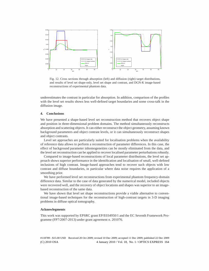
The reconstruction results are shown in the left and middle column of images in Fig. 11.Both reconstructions recover object and shape locations well. The combined shape and contrastreconstruction shows a small crosstalk artefact in the diffusion image located at the position ofthe absorbing inclusion. It also slightly overestimates the object sizes compared to the shape-only reconstruction, and in turn underestimates the objectcontrasts, as can be seen in the lineprofiles of recovered contrast levels in Fig. 12.

b) Comparison with Gauss-Newton-Krylov image-based reconstructions. For compari-son of the shape-based level set method with a voxel-based method, we performed a reconstruc-tion using the DGN-K solver with the phantom difference data. The right column of images inFigure 11 shows the reconstruction results, displayed withthe same gray-scale range as thelevel set reconstructions. Line profiles through the targetobjects are shown in Fig. 12. The re-construction does recover the target locations for the absorption and diffusion inclusions, but



http://www.opticsexpress.org/viewmedia.cfm?URI=oe-18-1-164-3

0 10 20 30 40 50 600

0.002

0.004

0.006

0.008

0.01

0.012

0.014

0.016

pos

µ a

LS shape only

LS shape+contrast

DGN−K

target

0 10 20 30 40 50 600

0.05

0.1

0.15

0.2

0.25

0.3

0.35

pos

κ

LS shape only

LS shape+contrast

DGN−K

target

Fig. 12. Cross sections through absorption (left) and diffusion (right) target distributions,and results of level set shape-only, level set shape and contrast, and DGN-K image-basedreconstructions of experimental phantom data.

underestimates the contrast in particular for absorption.In addition, comparison of the profileswith the level set results shows less well-defined target boundaries and some cross-talk in thediffusion image.

4. Conclusions

We have presented a shape-based level set reconstruction method that recovers object shapeand position in three-dimensional problem domains. The method simultaneously reconstructsabsorption and scattering objects. It can either reconstruct the object geometry, assuming knownbackground parameters and object contrast levels, or it cansimultaneously reconstruct shapesand object contrasts.

Level set approaches are particularly suited for localisation problems when the availabilityof reference data allows to perform a reconstruction of parameter differences. In this case, theeffect of background parameter inhomogeneities can be mostly eliminated from the data, andthe level set reconstruction can be applied to recover localised parameter perturbations robustly.

Compared to image-based reconstructions of local parameter distributions, the level set ap-proach shows superior performance in the identification andlocalisation of small, well-definedinclusions of high contrast. Image-based approaches tend to recover such objects with lowcontrast and diffuse boundaries, in particular where data noise requires the application of asmoothing prior.

We have performed level set reconstructions from experimental phantom frequency-domaindifference data. Similar to the case of data generated by thenumerical model, included objectswere recovered well, and the recovery of object locations and shapes was superior to an image-based reconstruction of the same data.

We have shown that level set shape reconstructions provide aviable alternative to conven-tional image-based techniques for the reconstruction of high-contrast targets in 3-D imagingproblems in diffuse optical tomography.

Acknowlegments

This work was supported by EPSRC grant EP/E034950/1 and the EC Seventh Framework Pro-gramme (FP7/2007-2013) under grant agreement n. 201076.



3D level set reconstruction of model and experimental data in Diffuse Optical Tomography

Documents

Transcript of 3D level set reconstruction of model and experimental data in Diffuse Optical Tomography