Three-dimensional volume-averaged soil moisture

transport model with a scalable parameterization of

subgrid topographic variability

Hyun I. Choi,1 Praveen Kumar,1 and Xin-Zhong Liang2

Received 28 April 2006; revised 20 September 2006; accepted 18 October 2006; published 11 April 2007.

[1] Subgrid variability of subsurface moisture flux transport is strongly influenced by thelocal variation of topographic attributes, such as elevation, slope, and curvature. A three-dimensional volume-averaged soil moisture transport (VAST) model is developed toincorporate these effects using the volume-averaged Richards equation. The small-perturbation approach is used to decompose the equation into mean and fluctuation, whichare then averaged over the model grid box. This formulation explicitly incorporates thevariability of moisture flux due to subgrid variation of topographic attributes. The model isindependent of scale, but the parameters need to be estimated at the model scale. It isdemonstrated that the flux contribution from the subgrid variability can be comparable tothat of mean flux, particularly under drier moisture conditions. This formulation can besubstituted for subsurface moisture transport schemes in most existing land surfacemodels.

Citation: Choi, H. I., P. Kumar, and X.-Z. Liang (2007), Three-dimensional volume-averaged soil moisture transport model with a

scalable parameterization of subgrid topographic variability, Water Resour. Res., 43, W04414, doi:10.1029/2006WR005134.

1. Introduction

[2] Climate models, both global and regional, have in-creased in physical sophistication and resolution. As a keycomponent, the land surface models (LSMs) have alsoevolved from simple bucket models (first generation) toinclude simple canopy models (second generation), photo-synthesis models (third generation), and dynamic vegetationmodels (fourth generation) [Gochis et al., 2004]. The fifthgeneration models need to incorporate more sophisticatedlinkages and process interactions at small scales to representtheir aggregated effect on larger scales. This requiresimprovements in parameterizing key subgrid processes.The effect of the heterogeneity of land surface processesdepends on the spatial variability of soil water that resultsfrom interactions between moisture flux and a variety offactors such as soil, vegetation, precipitation, evapotranspi-ration, topography, etc. In particular, topographic attributessuch as elevation, slope, curvature, and aspect introducesignificant variability at small scales that need to beaccounted for in terrestrial hydrologic models. CurrentLSMs usually incorporate the heterogeneity of local controls[Grayson et al., 1997] by dividing a grid (or a basin) intomosaic subregions. However, heterogeneity effects inducedby topographic characteristics within a model grid are poorlymodeled or totally neglected in most existing LSMs,although topographic data are readily available at fine

resolution (<1 km) over the globe. For instance, thethree-dimensional Richards equation can include topo-graphic features, but they are neglected in one-dimensionalsoil moisture transport equations used in most LSMs. Theseeffects are critical for subsurface moisture predictions. Theirincomplete representation causes significant biases in landsurface water and energy budget and consequently inregional climate simulations.[3] Effects of subgrid topographic variability on surface-

atmosphere interactions have been partially incorporated inthe basin-scale hydrologic models, such as ‘‘catchment’’model of Koster et al. [2000] and ‘‘large area basin scale’’model of Chen and Kumar [2001]. The basin-scale repre-sentation improves the modeling of lateral subsurface flowand spatial heterogeneities induced by soil moisture vari-ability. Chen and Kumar [2001, 2002, 2004] demonstratedthat incorporation of subgrid topographic attributes has asignificant impact on the water table dynamics and on thepredictability of soil moisture and surface energy balances.Consequently, interannual variations of deep layer soilmoisture and temperature are better characterized, especiallyover regions with El Nino–Southern Oscillation (ENSO)influence.[4] On the basis of these earlier studies, we start with the

hypothesis that topography is an important controllingfactor of subgrid moisture flux in large-scale land surfacesimulations. Kumar [2004] developed a new formulationbased on the Richards equation for the layer-averagedsubsurface moisture transport where explicit expressionswere derived for layer-averaged lateral transport contribu-tions due to topographic attributes, and showed that thelateral contributions can be a significant part of the total soilmoisture flux. A further development is offered here toderive the three-dimensional volume-averaged soil moisturetransport (VAST) equation by incorporating a parameteri-

1Environmental Hydrology and Hydraulic Engineering, Department ofCivil and Environmental Engineering, University of Illinois at Urbana-Champaign, Urbana, Illinois, USA.

2Center for Atmospheric Science, Illinois State Water Survey, Universityof Illinois, Champaign, Illinois, USA.

Copyright 2007 by the American Geophysical Union.0043-1397/07/2006WR005134$09.00

W04414

WATER RESOURCES RESEARCH, VOL. 43, W04414, doi:10.1029/2006WR005134, 2007ClickHere

for

FullArticle

1 of 15

zation of subgrid topographic effects, which is suitable forapplications at a range of regional climate model (RCM)scales. This VAST formulation, with the scalable parame-terization pertaining to subgrid variability effects, can besubstituted for the existing moisture transport scheme inmost existing LSMs. The VAST formulation also predictsthe grid mean directional lateral flow controlled by topo-graphic attributes from the bulk of each side of a grid box atindividual soil layers. For more realistic representation ofthe total lateral runoff, this subsurface lateral flow can bereadily combined with the surface runoff through a con-junctive flow modeling scheme (to be published in a futurepaper).[5] The Richards equation can be decomposed into the

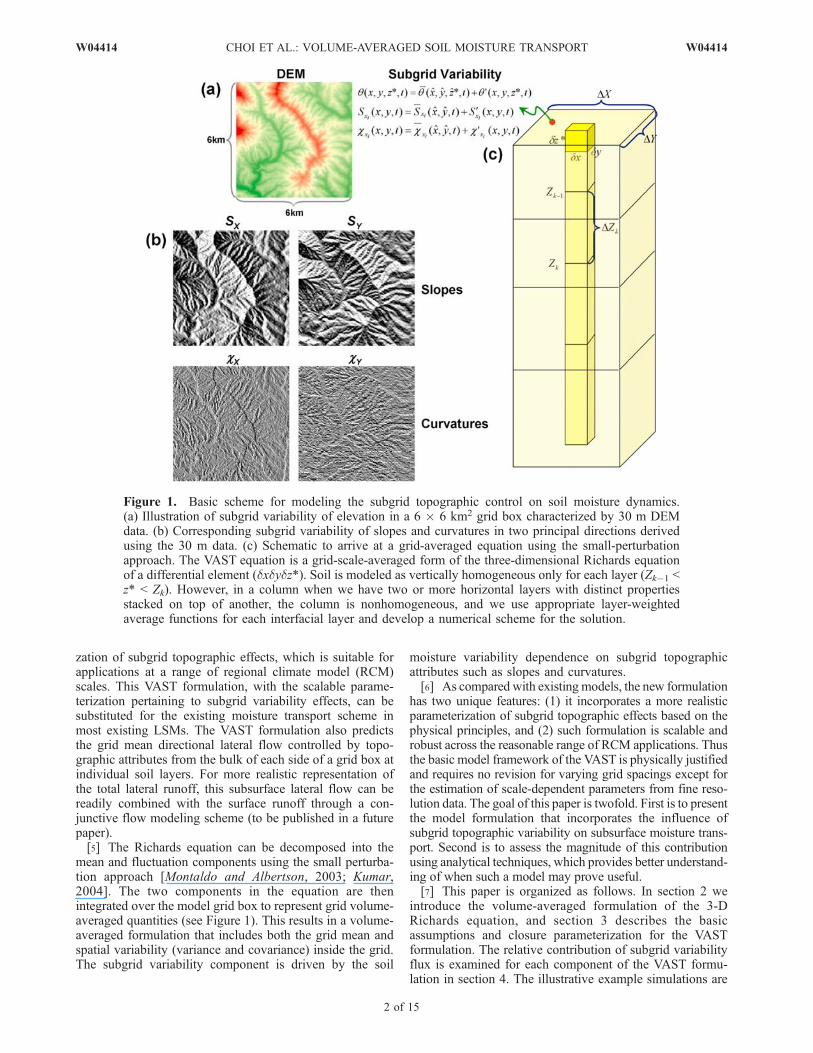
mean and fluctuation components using the small perturba-tion approach [Montaldo and Albertson, 2003; Kumar,2004]. The two components in the equation are thenintegrated over the model grid box to represent grid volume-averaged quantities (see Figure 1). This results in a volume-averaged formulation that includes both the grid mean andspatial variability (variance and covariance) inside the grid.The subgrid variability component is driven by the soil

moisture variability dependence on subgrid topographicattributes such as slopes and curvatures.[6] As compared with existing models, the new formulation

has two unique features: (1) it incorporates a more realisticparameterization of subgrid topographic effects based on thephysical principles, and (2) such formulation is scalable androbust across the reasonable range of RCM applications. Thusthe basic model framework of the VAST is physically justifiedand requires no revision for varying grid spacings except forthe estimation of scale-dependent parameters from fine reso-lution data. The goal of this paper is twofold. First is to presentthe model formulation that incorporates the influence ofsubgrid topographic variability on subsurface moisture trans-port. Second is to assess the magnitude of this contributionusing analytical techniques, which provides better understand-ing of when such a model may prove useful.[7] This paper is organized as follows. In section 2 we

introduce the volume-averaged formulation of the 3-DRichards equation, and section 3 describes the basicassumptions and closure parameterization for the VASTformulation. The relative contribution of subgrid variabilityflux is examined for each component of the VAST formu-lation in section 4. The illustrative example simulations are

Figure 1. Basic scheme for modeling the subgrid topographic control on soil moisture dynamics.(a) Illustration of subgrid variability of elevation in a 6 � 6 km2 grid box characterized by 30 m DEMdata. (b) Corresponding subgrid variability of slopes and curvatures in two principal directions derivedusing the 30 m data. (c) Schematic to arrive at a grid-averaged equation using the small-perturbationapproach. The VAST equation is a grid-scale-averaged form of the three-dimensional Richards equationof a differential element (dxdydz*). Soil is modeled as vertically homogeneous only for each layer (Zk�1 <z* < Zk). However, in a column when we have two or more horizontal layers with distinct propertiesstacked on top of another, the column is nonhomogeneous, and we use appropriate layer-weightedaverage functions for each interfacial layer and develop a numerical scheme for the solution.

2 of 15

W04414 CHOI ET AL.: VOLUME-AVERAGED SOIL MOISTURE TRANSPORT W04414

described in section 5, and summary and conclusions aregiven in section 6.

2. VAST Model Formulation

[8] We start with the Richards equation, most often usedfor the soil moisture transport model on the Cartesiancoordinate system as

@q@t

¼ @

@xiKxi yð Þ @h

@xi

� �; ð1Þ

where q is the volumetric soil moisture content, t is time, andthe summation over the coordinates xi 2 {x, y, z} is implied;x � y represents the horizontal plane, and z is the verticalaxis. Kxi

(y) is the hydraulic conductivity at the suction heady, and h is the total head written as h = y + z. Here we do notpresent any source and sink terms, such as evapotranspira-tion, redistribution by plant roots, well pumping and so on,which can be incorporated as necessary through an externalterm or a boundary condition in the solution of this equation.To facilitate incorporating topographic effects we introducethe terrain-following vertical coordinate z* expressed asz* = ZG � z where ZG is the ground surface elevation. Thiscoordinate system can explicitly incorporate topographiceffects on the Richards equation as below:

@q@t

¼ @

@xl*Dxl*

qð Þ @q@xl*

þ Kxl*qð ÞSxl*

� �; ð2Þ

where x*l 2 {x, y, z*} is the new coordinate system, and

Dxl*(q) = Kxl*(q)@y@q is the diffusivity. The local terrain surface

slopes Sxl* are (Sx, Sy, Sz*) = (@ZG@x ,@ZG@y , �1).

[9] For any variable F , a volume-averaged quantity F isdefined as

F xl*; tð Þ ¼ 1

V

ZV

F xl*; tð Þ dV ; ð3Þ

where V denotes the volume of a computational grid box,and x*l 2 {x, y, z*} is the center of the grid. The variable Fcan then be decomposed into the volume average andperturbation components as

F xl*; tð Þ ¼ F xl*; tð Þ þ F 0 xl*; tð Þ: ð4Þ

[10] For the soil moisture q at any local point within thegrid box we have q(x*l , t) = q(x*l, t) + q0(x*l, t). Note thatthe hydraulic conductivity and diffusivity are dependent onthe soil properties as well as soil moisture (see section 3). Todevelop the framework for the soil moisture redistributiondriven by topography, we focus on the contributions of thesoil moisture heterogeneity induced by topography withinthe grid volume and assume that the effect of subgridvariability of soil properties and their covariances with thesoil moisture are secondary (see section 3). With thisassumption, equation (2) can be decomposed as

@q@t

þ @q0

@t¼ @

@xl*Dxl*

qþ q0� � @q

@xl*þ @q0

@xl*

� ��

þ Kxl*qþ q0� �

Sxl* þ S0xl*

� �; ð5Þ

where the slope term is also decomposed as Sxl* (x*l, t) = Sxl*(x*l, t) + S0xl* (x*l, t). Note that topographic attributes such as

slopes and curvatures are independent of vertical coordinatez*.[11] Using the second-order Taylor series expansion, Kxl*

and Dxl* terms are approximated as

Kxl*

�qþ q0� �

Kxl*

�q� �

þ@K

xl*

@qj�qq

0 þ 1

2

@2Kxl*

@q2j�qq0

2; ð6Þ

Dxl*

�qþ q0� �

Dxl*

�q� �

þ@D

xl*

@qj�qq

0 þ 1

2

@2Dxl*

@q2j�qq0

2: ð7Þ

[12] We define symbol notations for the above derivative

terms as _Kxl*(q) �@K

xl*

@q jq, _Dxl*(q) �@D

xl*

@q jq, �Kxl*(q) �@2K

xl*

@q2jq,

and �Dx*l(q) �

@2Dxl*

@q2jq.

[13] Substituting equations (6) and (7) into equation (5)and expanding give

@q@t

þ @q0

@t¼ @

@xl*Dxl*

q� � @q

@xl*þ Dxl*

q� � @q0

@xl*

� �

þ @

@xl*_Dxl*

q� � @q

@xl*q0 þ 1

2_Dxl*

q� � @q02

@xl*

" #

þ @

@xl*1

2�Dxl*

q� � @q

@xl*q02 þ 1

6�Dxl*

q� � @q03

@xl*

" #

þ @

@xl*Kxl*

q� �

Sxl*þ K

xl*q� �

S0xl*

h iþ @

@xl*_Kxl*

q� �

Sxl*q0 þ _K

xl*q� �

q0S0xl*

h iþ @

@xl*1

2�Kxl*

q� �

Sxl*q02 þ 1

2�Kxl*

q� �

q02S0xl*

� �: ð8Þ

[14] Neglecting the third-order terms (16�Dxl*(q)

@q03

@xl*and

12�Kxl*(q)q

02 S0xl*), and taking a volume integral over the grid

box using q0 = 0 and q0 2 � sq2 in equation (8), we obtain

@q@t

¼ @

@xl*Dxl*

q� � @q

@xl*þ 1

2_Dxl*

q� � @s2

q

@xl*þ 1

2�Dxl*

q� � @q

@xl*s2q

� �

þ @

@xl*Kxl*

q� �

Sxl*þ _K

xl*q� �

q0S0xl*þ 1

2�Kxl*

q� �

Sxl*s2q

� �; ð9Þ

where q0S0xl*

is the covariance between soil moisture andterrain slope.[15] Using 1

2[ _Dxl*(q)

@s2q

@xl*+ �Dxl*(q) sq

2 @q@xl*

]� 12

@@xl*

[ _Dxl*(q)sq2]

and separating the vertical and lateral terms, we finally obtain

the volume average 3-D Richards equation as

@�q@t

¼ @

@z*Dz*

�q� � @�q

@z*

� �|fflfflfflfflfflfflfflfflfflfflfflfflffl{zfflfflfflfflfflfflfflfflfflfflfflfflffl}

mean term

þ 1

2

@2

@z*2_Dz*

�q� �

s2q

� �|fflfflfflfflfflfflfflfflfflfflfflfflfflffl{zfflfflfflfflfflfflfflfflfflfflfflfflfflffl}

variability term

Vertical Diffusion½ �

� @

@z*Kz*

�q� �� �

|fflfflfflfflfflfflfflfflffl{zfflfflfflfflfflfflfflfflffl}mean term

� 1

2

@

@z*�Kz*

�q� �

s2q

� �|fflfflfflfflfflfflfflfflfflfflfflfflffl{zfflfflfflfflfflfflfflfflfflfflfflfflffl}

variability term

Vertical Drainage½ �

þ @

@xlDxl

�q� � @�q

@xl

� �|fflfflfflfflfflfflfflfflfflfflfflffl{zfflfflfflfflfflfflfflfflfflfflfflffl}

mean term

þ 1

2

@2

@x2l_Dxl

�q� �

s2q

� �|fflfflfflfflfflfflfflfflfflfflfflffl{zfflfflfflfflfflfflfflfflfflfflfflffl}

variability term

Lateral Diffusion½ �

þ @

@xlKxl

�q� �

�Sxl� �

|fflfflfflfflfflfflfflfflfflfflffl{zfflfflfflfflfflfflfflfflfflfflffl}mean term

þ @

@xl_Kxl

�q� �

q0S0xl

h iþ 1

2

@

@xl�Kxl

�q� �

�Sxls2q

� �|fflfflfflfflfflfflfflfflfflfflfflfflfflfflfflfflfflfflfflfflfflfflfflfflfflfflfflfflfflfflfflfflfflffl{zfflfflfflfflfflfflfflfflfflfflfflfflfflfflfflfflfflfflfflfflfflfflfflfflfflfflfflfflfflfflfflfflfflffl}

variability term

;

Lateral Drainage½ �ð10Þ

W04414 CHOI ET AL.: VOLUME-AVERAGED SOIL MOISTURE TRANSPORT

3 of 15

W04414

where xl 2 {x, y}, and we have used Sz* = �1 and q0S0z* = 0since S0z* � 0 in the vertical drainage component. Note thatthis formulation includes unknown variance sq

2 andcovariance q0S0xl that require an appropriate closure para-meterization as presented in section 3.[16] Equation (10) incorporates both the grid mean and

variability flux terms for each vertical and lateral compo-nent while most current LSMs consider only the verticalmean flux terms. Kumar [2004] introduced the layer-averagedRichards equation that includes the mean vertical andlateral flux terms. None of previous LSMs, however,explicitly incorporates the variability flux terms due tosubgrid soil moisture and terrain heterogeneity. The relativecontribution of each additional variability term is evaluatedin section 4.[17] To simplify notation, all volume-averaged variables

and coefficients are defined at the center of a grid volumethroughout this paper, unless specifically noted otherwise.

3. Approximations and ClosureParameterizations

[18] To make equation (10) more tractable, the followingassumptions are adopted.[19] 1. The Brooks and Corey [1964] relations generally

apply:

K qð Þ ¼ Ks

qqs

� �2bþ3

; ð11Þ

y qð Þ ¼ ys

qqs

� ��b

; ð12Þ

where Ks, ys, qs are the hydraulic conductivity, the suctionhead, and the soil moisture content at saturation, respec-tively. These parameters and the exponent b characterize thekey soil hydraulic properties.[20] 2. The soil properties, Ks, ys, qs, and b, are assumed

to be constant and uncorrelated with each other within a gridvolume. Their representative values were given by Clappand Hornberger [1978] for 11 typical soil texture types, andcan be also approximated by pedotransfer functions in termsof soil sand and clay fractions [Cosby et al., 1984]. Whilefine resolution data of the digital elevation model (DEM)are available for parameterizing the dependence of subgridsoil moisture on topography, no such data is available forsoil properties. Consequently only subgrid variability due totopographic control on moisture transport is incorporated inthe model. Note, however, that soil properties can stillchange from grid element to grid element, both verticallyand horizontally.[21] 3. The vertical saturated hydraulic conductivity is

relaxed to incorporate the dependence on soil depth. Follow-ing the TOPMODEL formulation [Beven and Kirkby, 1979],most recent studies assume an exponential decay function:

Ksz*¼ K0e

�f z*�Zrð Þ: ð13Þ

where Ksz*is the vertical saturated hydraulic conductivity,

K0 is its value at a reference depth Zr, and f is an exponentdecay factor whose range from published literatures wassummarized in Table 1 of Kumar [2004].

[22] Following the assumption 2, we use a grid represen-tative value by layer averaging as

Ksz* 1

DZk

Z Zk

Zk�1

K0e�f z*�Zrð Þ dz ¼ K0

e�f Zk�Zrð Þ

fDZkefDZk � 1� �

;

ð14Þ

where DZk is a layer thickness between vertical coordinatesZk and Zk�1. As such the Ksz*

is treated constant within thegrid volume, but can vary from one grid element to nextvertically and horizontally. Hence a proper averagingmethod is required to estimate the effective saturatedconductivity at each interface between the two adjacentvertical layers and horizontal grids for the numericalsolution of the VAST model.[23] 4. The lateral hydraulic conductivity is larger than

vertical to account for anisotropy [Freeze and Cherry,1979]:

Ksx ¼ Ksy ¼ zKsz*; ð15Þ

where z is the anisotropic ratio; see Table 2 of Kumar[2004] for a compilation of values from published literature.[24] These assumptions together lead to

Kxl*

�q� �

¼ Ksxl*

�qqs

� �2bþ3

; ð16Þ

_Kxl*

�q� �

¼Ks

xl*2bþ 3ð Þ

qs

�qqs

� �2bþ2

; ð17Þ

�Kxl*

�q� �

¼Ks

xl*2bþ 2ð Þ 2bþ 3ð Þ

q2s

�qqs

� �2bþ1

; ð18Þ

Dxl*

�q� �

¼ �Ks

xl*ysb

qs

�qqs

� �bþ2

; ð19Þ

_Dxl*

�q� �

¼ �Ks

xl*ysb bþ 2ð Þ

q2s

�qqs

� �bþ1

; ð20Þ

�Dxl*

�q� �

¼ �Ks

xl*ysb bþ 1ð Þ bþ 2ð Þ

q3s

�qqs

� �b

: ð21Þ

[25] 5. Figure 1 and Table 3 of Kumar [2004] show thesoil moisture variability from published data. FollowingKumar [2004], we parameterize the unknown variable squsing the field measurement data. We use the SouthernGreat Plains 1997 (SGP97) Hydrology Experiment data from6 sites each containing 27–49 samples between 18 Juneand 17 July 1997 [Famiglietti et al., 1999]. The soil texture(and so qs) is uniform within each site but differs betweensites. The topography is flat to gently rolling, and thus itsslope effect on soil moisture is small.[26] Famiglietti et al. [1999] showed that the coefficient

of variance Cv = sq�q

distinctly decreases as mean soilmoisture increases. On the other hand, as shown inFigure 2, the fitting to observations gives

Cv ¼a

�q=qs� �b ; ð22Þ

4 of 15

W04414 CHOI ET AL.: VOLUME-AVERAGED SOIL MOISTURE TRANSPORT W04414

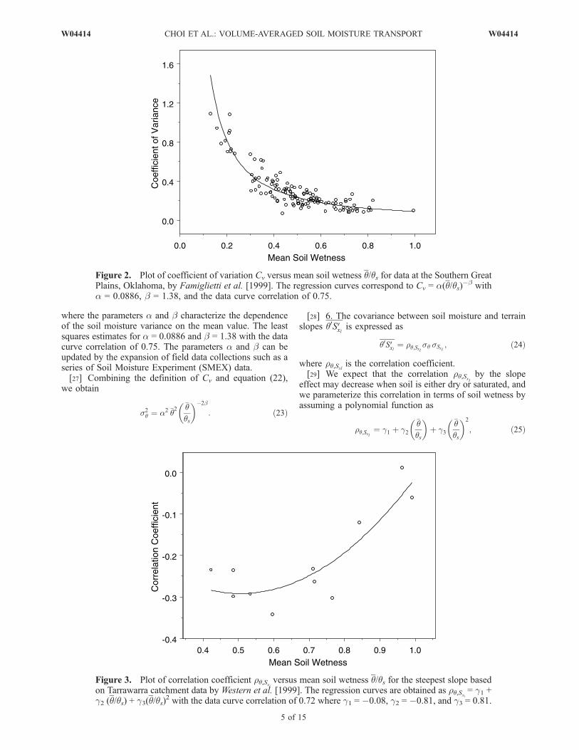
where the parameters a and b characterize the dependenceof the soil moisture variance on the mean value. The leastsquares estimates for a = 0.0886 and b = 1.38 with the datacurve correlation of 0.75. The parameters a and b can beupdated by the expansion of field data collections such as aseries of Soil Moisture Experiment (SMEX) data.[27] Combining the definition of Cv and equation (22),

we obtain

s2q ¼ a2 �q2

�qqs

� ��2b

: ð23Þ

[28] 6. The covariance between soil moisture and terrainslopes q0S0xl is expressed as

q0S0xl ¼ rq;Sxl sq sSxl; ð24Þ

where rq,Sxl is the correlation coefficient.[29] We expect that the correlation rq,Sx

l

by the slopeeffect may decrease when soil is either dry or saturated, andwe parameterize this correlation in terms of soil wetness byassuming a polynomial function as

rq;Sxl ¼ g1 þ g2�qqs

� �þ g3

�qqs

� �2

; ð25Þ

Figure 2. Plot of coefficient of variation Cv versus mean soil wetness q/qs for data at the Southern GreatPlains, Oklahoma, by Famiglietti et al. [1999]. The regression curves correspond to Cv = a(q/qs)

�b witha = 0.0886, b = 1.38, and the data curve correlation of 0.75.

Figure 3. Plot of correlation coefficient rq,Sxl versus mean soil wetness q/qs for the steepest slope basedon Tarrawarra catchment data by Western et al. [1999]. The regression curves are obtained as rq,Sxl = g1 +g2 (q/qs) + g3(q/qs)

2 with the data curve correlation of 0.72 where g1 = �0.08, g2 = �0.81, and g3 = 0.81.

W04414 CHOI ET AL.: VOLUME-AVERAGED SOIL MOISTURE TRANSPORT

5 of 15

W04414

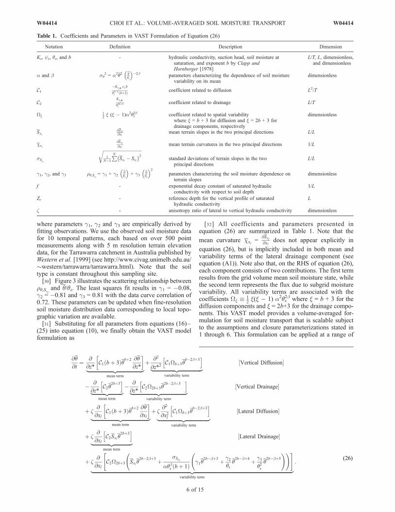
where parameters g1, g2 and g3 are empirically derived byfitting observations. We use the observed soil moisture datafor 10 temporal patterns, each based on over 500 pointmeasurements along with 5 m resolution terrain elevationdata, for the Tarrawarra catchment in Australia published byWestern et al. [1999] (see http://www.civag.unimelb.edu.au/�western/tarrawarra/tarrawarra.html). Note that the soiltype is constant throughout this sampling site.[30] Figure 3 illustrates the scattering relationship between

rq,Sxl

and q/qs. The least squares fit results in g1 = �0.08,g2 = �0.81 and g3 = 0.81 with the data curve correlation of0.72. These parameters can be updated when fine-resolutionsoil moisture distribution data corresponding to local topo-graphic variation are available.[31] Substituting for all parameters from equations (16)–

(25) into equation (10), we finally obtain the VAST modelformulation as

@q@t

¼ @

@z*C1 bþ 3ð Þqbþ2 @q

@z*

� �|fflfflfflfflfflfflfflfflfflfflfflfflfflfflfflfflfflfflfflffl{zfflfflfflfflfflfflfflfflfflfflfflfflfflfflfflfflfflfflfflffl}

mean term

þ @2

@z*2C1Wbþ3q

b�2bþ3h i

|fflfflfflfflfflfflfflfflfflfflfflfflfflfflfflfflfflffl{zfflfflfflfflfflfflfflfflfflfflfflfflfflfflfflfflfflffl}variability term

Vertical Diffusion½ �

� @

@z*C2q

2bþ3h i

|fflfflfflfflfflfflfflfflfflffl{zfflfflfflfflfflfflfflfflfflffl}mean term

� @

@z*C2W2bþ3q

2b�2bþ3h i

|fflfflfflfflfflfflfflfflfflfflfflfflfflfflfflfflfflfflfflffl{zfflfflfflfflfflfflfflfflfflfflfflfflfflfflfflfflfflfflfflffl}variability term

Vertical Drainage½ �

þ z@

@xlC1 bþ 3ð Þqbþ2 @q

@xl

� �|fflfflfflfflfflfflfflfflfflfflfflfflfflfflfflfflfflfflfflfflffl{zfflfflfflfflfflfflfflfflfflfflfflfflfflfflfflfflfflfflfflfflffl}

mean term

þ z@2

@x2lC1Wbþ3q

b�2bþ3h i

|fflfflfflfflfflfflfflfflfflfflfflfflfflfflfflfflfflffl{zfflfflfflfflfflfflfflfflfflfflfflfflfflfflfflfflfflffl}variability term

Lateral Diffusion½ �

þ z@

@xlC2Sxlq

2bþ3h i

|fflfflfflfflfflfflfflfflfflfflfflfflfflffl{zfflfflfflfflfflfflfflfflfflfflfflfflfflffl}mean term

Lateral Drainage½ �

þ z@

@xlC2W2bþ3 Sxlq

2b�2bþ3 þsSxl

aqbs bþ 1ð Þg1q

2b�bþ3 þ g2qs

q2b�bþ4 þ g3

q2sq2b�bþ5

! !" #|fflfflfflfflfflfflfflfflfflfflfflfflfflfflfflfflfflfflfflfflfflfflfflfflfflfflfflfflfflfflfflfflfflfflfflfflfflfflfflfflfflfflfflfflfflfflfflfflfflfflfflfflfflfflfflfflfflfflfflfflfflfflfflfflfflfflfflfflfflfflfflfflfflfflfflfflfflfflfflffl{zfflfflfflfflfflfflfflfflfflfflfflfflfflfflfflfflfflfflfflfflfflfflfflfflfflfflfflfflfflfflfflfflfflfflfflfflfflfflfflfflfflfflfflfflfflfflfflfflfflfflfflfflfflfflfflfflfflfflfflfflfflfflfflfflfflfflfflfflfflfflfflfflfflfflfflfflfflfflfflffl}

variability term

:

[32] All coefficients and parameters presented inequation (26) are summarized in Table 1. Note that the

mean curvature cxl=

@Sxl@xl

does not appear explicitly in

equation (26), but is implicitly included in both mean andvariability terms of the lateral drainage component (seeequation (A1)). Note also that, on the RHS of equation (26),each component consists of two contributions. The first termresults from the grid volume mean soil moisture state, whilethe second term represents the flux due to subgrid moisturevariability. All variability terms are associated with thecoefficients Wx � 1

2x(x � 1) a2qs

2b where x = b + 3 for thediffusion components and x = 2b+3 for the drainage compo-nents. This VAST model provides a volume-averaged for-mulation for soil moisture transport that is scalable subjectto the assumptions and closure parameterizations stated in1 through 6. This formulation can be applied at a range of

Table 1. Coefficients and Parameters in VAST Formulation of Equation (26)

Notation Definition Description Dimension

Ks, ys, qs, and b - hydraulic conductivity, suction head, soil moisture atsaturation, and exponent b by Clapp andHornberger [1978]

L/T, L, dimensionless,and dimensionless

a and b sq2 = a2q2 q

qs

� �2b parameters characterizing the dependence of soil moisture

variability on its meandimensionless

C1�Ks

z*ysb

qbþ3s bþ3ð Þ coefficient related to diffusion L2/T

C2Ks

z*q2bþ3s

coefficient related to drainage L/T

Wx12x (x � 1)a2q2s

b coefficient related to spatial variabilitywhere x = b + 3 for diffusion and x = 2b + 3 fordrainage components, respectively

dimensionless

Sxl@ZG

@xlmean terrain slopes in the two principal directions L/L

cxl

@Sxl@xl

mean terrain curvatures in the two principal directions 1/L

sSxl

ffiffiffiffiffiffiffiffiffiffiffiffiffiffiffiffiffiffiffiffiffiffiffiffiffiffiffiffiffiffiffiffiffiffiffiffi1

N�1

PNSxl � Sxl� �2r

standard deviations of terrain slopes in the twoprincipal directions

L/L

g1, g2, and g3 rq,Sxl = g1 + g2 qqs

� + g3 q

qs

� 2parameters characterizing the soil moisture dependence onterrain slopes

dimensionless

f - exponential decay constant of saturated hydraulicconductivity with respect to soil depth

1/L

Zr - reference depth for the vertical profile of saturatedhydraulic conductivity

L

z - anisotropy ratio of lateral to vertical hydraulic conductivity dimensionless

(26)

6 of 15

W04414 CHOI ET AL.: VOLUME-AVERAGED SOIL MOISTURE TRANSPORT W04414

scales with appropriate estimation of scale-dependent param-eters. Any source and sink terms at the scale of an averaginggrid volume can be incorporated in this VAST formulation asan external term or a boundary condition in land surfacemodels.

4. Relative Contribution of Subgrid Variability

[33] The VAST model consists of the grid mean andsubgrid variability terms induced by topographic attributessuch as slopes and curvatures. We now use this formulationto gain an insight into the relative contribution of eachvariability flux term introduced in this formulation, whichis generally not represented in most current LSMs. Thefollowing focuses on the relative contributions of the subgridvariability versus the grid mean components under differentmoisture states. Analysis is performed on the assumptionthat soil properties, Ks, ys, qs, and b, are constant throughoutthe entire soil column. Although this assumption is notrequired in the VAST model formulation, it enables us to

analytically evaluate the subgrid variability effects that resultfrom only topographic variations. The relative ratios ofsubgrid to mean fluxes are summarized in Table 2, and theirdetailed derivations are given in Appendix A.[34] The analysis takes into account a range of soil mois-

ture values from hygroscopic water (y ’ �3100 kPa),permanent wilting point (y’�1500 kPa), and field capacity(y’�34 kPa), to saturation (y ’ 0 kPa). The soil wetnessq/qs is then calculated using the Brooks and Corey [1964]relation in equation (12) and soil properties ys and b for11 typical soil textures fromClapp and Hornberger [1978] tocompare the relative contribution ratios for various soil types.[35] Besides q, a, b, qs and b, the lateral contribution

ratios RL2,1and RL2,2

(Table 2) incorporate additional param-

eters g1, g2, g3, sSxl/Sxl, and@sSxl

@xl/cxl

, which are associated

with subgrid topographic variability. The topographic attri-

bute ratios sSxl/Sxl and@sSxl

@xl/cxl

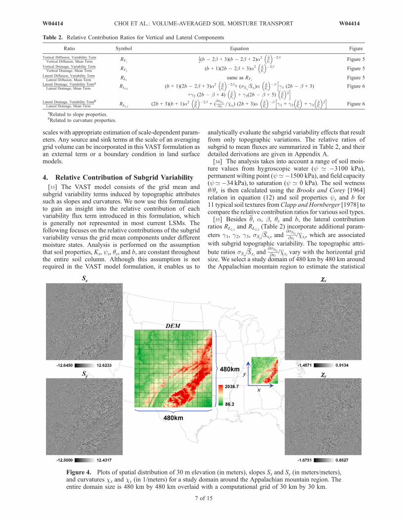
vary with the horizontal gridsize. We select a study domain of 480 km by 480 km aroundthe Appalachian mountain region to estimate the statistical

Table 2. Relative Contribution Ratios for Vertical and Lateral Components

Ratio Symbol Equation Figure

Vertical Diffusion; Variability TermVertical Diffusion; Mean Term

RV1

12(b � 2b + 3)(b � 2b + 2)a2 �q

qs

� �2b Figure 5

Vertical Drainage; Variability TermVertical Drainage; Mean Term

RV2(b + 1)(2b � 2b + 3)a2 �q

qs

� �2b Figure 5

Lateral Diffusion; Variability TermLateral Diffusion; Mean Term

RL1same as RV1

Figure 5

Lateral Drainage; Variability TermLateral Drainage; Mean Term

aRL2,1

(b + 1)(2b � 2b + 3)a2 �qqs

� �2b+ (sSxl /

�Sxl)a�qqs

� �bhg1 (2b � b + 3)

+g2 (2b � b + 4)�qqs

� + g3(2b � b + 5)

�qqs

� 2i Figure 6

Lateral Drainage; Variability TermLateral Drainage; Mean Term

bRL2,2

(2b + 3)(b + 1)a2 �qqs

� �2b + (

@sSxl

@xl=�cxl

) (2b + 3)a �qqs

� �bhg1 + g2

�qqs

� + g3

�qqs

� 2i

Figure 6

aRelated to slope properties.bRelated to curvature properties.

Figure 4. Plots of spatial distribution of 30 m elevation (in meters), slopes Sx and Sy (in meters/meters),and curvatures cx and cy (in 1/meters) for a study domain around the Appalachian mountain region. Theentire domain size is 480 km by 480 km overlaid with a computational grid of 30 km by 30 km.

W04414 CHOI ET AL.: VOLUME-AVERAGED SOIL MOISTURE TRANSPORT

7 of 15

W04414

properties of topographic attributes. Figure 4 illustrates thegeographic distributions of the terrain elevation, and slopesand curvatures in the two principal directions based on thecommercial seamless 30 m NED (National Elevation Data,http://ned.usgs.gov/). Given a specific grid scale, the meanelevation is first calculated and then the correspondingstatistical properties for topographic attributes, such as meanand standard deviation for slopes and curvatures, are calcu-lated by the central differencing scheme. Note that the two

topographic attribute ratios sSxl /Sxl and@sSxl

@xl/cxl

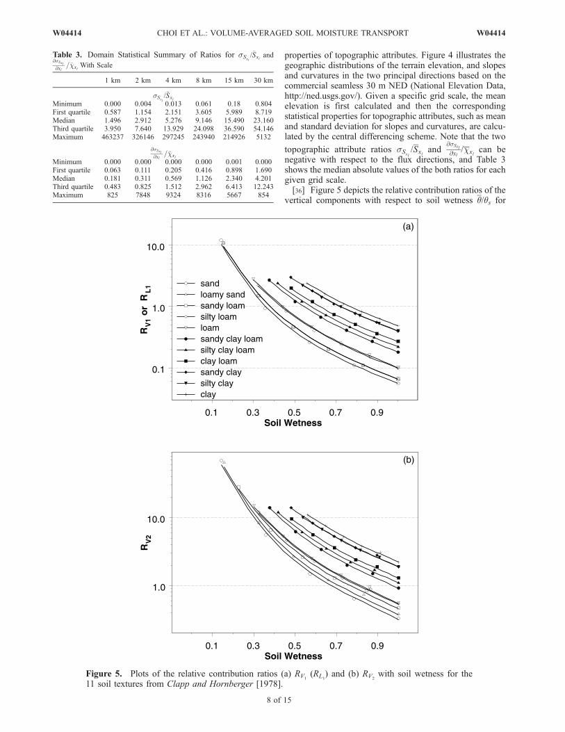
can benegative with respect to the flux directions, and Table 3shows the median absolute values of the both ratios for eachgiven grid scale.[36] Figure 5 depicts the relative contribution ratios of the

vertical components with respect to soil wetness q/qs for

Table 3. Domain Statistical Summary of Ratios for sSxl /�Sxl and

@sSxl

@xl=�cxl

With Scale

1 km 2 km 4 km 8 km 15 km 30 km

sSxl /�Sxl

Minimum 0.000 0.004 0.013 0.061 0.18 0.804First quartile 0.587 1.154 2.151 3.605 5.989 8.719Median 1.496 2.912 5.276 9.146 15.490 23.160Third quartile 3.950 7.640 13.929 24.098 36.590 54.146Maximum 463237 326146 297245 243940 214926 5132

@sSxl

@xl=�cxl

Minimum 0.000 0.000 0.000 0.000 0.001 0.000First quartile 0.063 0.111 0.205 0.416 0.898 1.690Median 0.181 0.311 0.569 1.126 2.340 4.201Third quartile 0.483 0.825 1.512 2.962 6.413 12.243Maximum 825 7848 9324 8316 5667 854

Figure 5. Plots of the relative contribution ratios (a) RV1(RL1

) and (b) RV2with soil wetness for the

11 soil textures from Clapp and Hornberger [1978].

8 of 15

W04414 CHOI ET AL.: VOLUME-AVERAGED SOIL MOISTURE TRANSPORT W04414

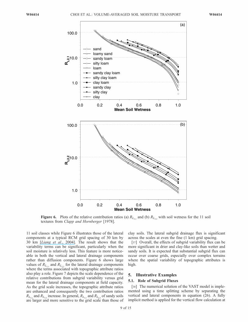
11 soil classes while Figure 6 illustrates those of the lateralcomponents at a typical RCM grid spacing of 30 km by30 km [Liang et al., 2004]. The result shows that thevariability terms can be significant, particularly when thesoil moisture is relatively less. This feature is more notice-able in both the vertical and lateral drainage componentsrather than diffusion components. Figure 6 shows largevalues of RL2,1

and RL2,2for the lateral drainage components

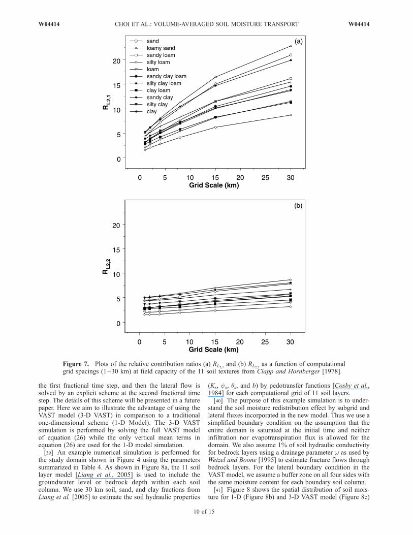
where the terms associated with topographic attribute ratiosalso play a role. Figure 7 depicts the scale dependence of therelative contributions from subgrid variability versus gridmean for the lateral drainage components at field capacity.As the grid scale increases, the topographic attribute ratiosare enhanced and consequently the two contribution ratiosRL2,1

and RL2,2increase. In general, RL2,1

and RL2,2of sandy soils

are larger and more sensitive to the grid scale than those of

clay soils. The lateral subgrid drainage flux is significantacross the scales at even the fine (1 km) grid spacing.[37] Overall, the effects of subgrid variability flux can be

more significant in drier and clay-like soils than wetter andsandy soils. It is expected that substantial subgrid flux canoccur over coarse grids, especially over complex terrainswhere the spatial variability of topographic attributes ishigh.

5. Illustrative Examples

5.1. Role of Subgrid Fluxes

[38] The numerical solution of the VAST model is imple-mented using a time splitting scheme by separating thevertical and lateral components in equation (26). A fullyimplicit method is applied for the vertical flow calculation at

Figure 6. Plots of the relative contribution ratios (a) RL2,1and (b) RL2,2

with soil wetness for the 11 soiltextures from Clapp and Hornberger [1978].

W04414 CHOI ET AL.: VOLUME-AVERAGED SOIL MOISTURE TRANSPORT

9 of 15

W04414

the first fractional time step, and then the lateral flow issolved by an explicit scheme at the second fractional timestep. The details of this scheme will be presented in a futurepaper. Here we aim to illustrate the advantage of using theVAST model (3-D VAST) in comparison to a traditionalone-dimensional scheme (1-D Model). The 3-D VASTsimulation is performed by solving the full VAST modelof equation (26) while the only vertical mean terms inequation (26) are used for the 1-D model simulation.[39] An example numerical simulation is performed for

the study domain shown in Figure 4 using the parameterssummarized in Table 4. As shown in Figure 8a, the 11 soillayer model [Liang et al., 2005] is used to include thegroundwater level or bedrock depth within each soilcolumn. We use 30 km soil, sand, and clay fractions fromLiang et al. [2005] to estimate the soil hydraulic properties

(Ks, ys, qs, and b) by pedotransfer functions [Cosby et al.,1984] for each computational grid of 11 soil layers.[40] The purpose of this example simulation is to under-

stand the soil moisture redistribution effect by subgrid andlateral fluxes incorporated in the new model. Thus we use asimplified boundary condition on the assumption that theentire domain is saturated at the initial time and neitherinfiltration nor evapotranspiration flux is allowed for thedomain. We also assume 1% of soil hydraulic conductivityfor bedrock layers using a drainage parameter w as used byWetzel and Boone [1995] to estimate fracture flows throughbedrock layers. For the lateral boundary condition in theVAST model, we assume a buffer zone on all four sides withthe same moisture content for each boundary soil column.[41] Figure 8 shows the spatial distribution of soil mois-

ture for 1-D (Figure 8b) and 3-D VAST model (Figure 8c)

Figure 7. Plots of the relative contribution ratios (a) RL2,1and (b) RL2,2

as a function of computationalgrid spacings (1–30 km) at field capacity of the 11 soil textures from Clapp and Hornberger [1978].

10 of 15

W04414 CHOI ET AL.: VOLUME-AVERAGED SOIL MOISTURE TRANSPORT W04414

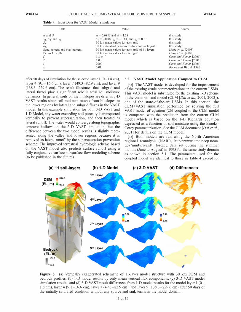
after 50 days of simulation for the selected layer 1 (0–1.8 cm),layer 4 (9.1–16.6 cm), layer 7 (49.3–82.9 cm), and layer 9(138.3–229.6 cm). The result illustrates that subgrid andlateral fluxes play a significant role in total soil moisturedynamics. In general, soils on the hillslopes are drier in 3-DVAST results since soil moisture moves from hillslopes tothe lower regions by lateral and subgrid fluxes in the VASTmodel. In this example simulation for both 3-D VAST and1-D Model, any water exceeding soil porosity is transportedvertically to prevent supersaturation, and then treated aslateral runoff. The water would converge along topographicconcave hollows in the 3-D VAST simulation, but thedifference between the two model results is slightly repre-sented along the valley and lower regions because it isremoved as lateral runoff by the supersaturation preventionscheme. The improved terrestrial hydrologic scheme basedon the VAST model also predicts surface runoff using afully conjunctive surface-subsurface flow modeling scheme(to be published in the future).

5.2. VAST Model Application Coupled to CLM

[42] The VAST model is developed for the improvementof the existing crude parameterizations in the current LSMs.This VAST model is substituted for the existing 1-D schemein the common land model (CLM [Dai et al., 2001, 2003]),one of the state-of-the-art LSMs. In this section, theCLM+VAST simulation performed by solving the fullVAST model of equation (26) coupled to the CLM modelis compared with the prediction from the current CLMmodel which is based on the 1-D Richards equationexpressed as a function of soil moisture using the Brooks-Corey parameterization. See the CLM document [Dai et al.,2001] for details on the CLM model.[43] Both models are run using the North American

regional reanalysis (NARR, http://www.emc.ncep.noaa.gov/mmb/rreanl/) forcing data set during the summermonths (June to August) in 1995 for the same study domainas shown in section 5.1. The parameters used for thecoupled model are identical to those in Table 4 except for

Table 4. Input Data for VAST Model Simulation

Data Value Source

a and b a = 0.0886 and b = 1.38 this studyg1, g2, and g3 g1 = �0.08, g2 = �0.81, and g3 = 0.81 this study�Sxl 30 km mean values for each grid this studysSxl 30 km standard deviation values for each grid this studySand percent and clay percent 30 km mean values for each grid of 11 layers Liang et al. [2005]Bedrock depth 30 km mean values for each grid Liang et al. [2005]f 1.8 m�1 Chen and Kumar [2001]Zr 1.0 m Chen and Kumar [2001]z 2000 Chen and Kumar [2001]w 0.01 Boone and Wetzel [1996]

Figure 8. (a) Vertically exaggerated schematic of 11-layer model structure with 30 km DEM andbedrock profiles, (b) 1-D model results by only mean vertical flux components, (c) 3-D VAST modelsimulation results, and (d) 3-D VAST result differences from 1-D model results for the model layer 1 (0–1.8 cm), layer 4 (9.1–16.6 cm), layer 7 (49.3–82.9 cm), and layer 9 (138.3–229.6 cm) after 50 days ofthe initially saturated condition without any source and sink terms in the model domain.

W04414 CHOI ET AL.: VOLUME-AVERAGED SOIL MOISTURE TRANSPORT

11 of 15

W04414

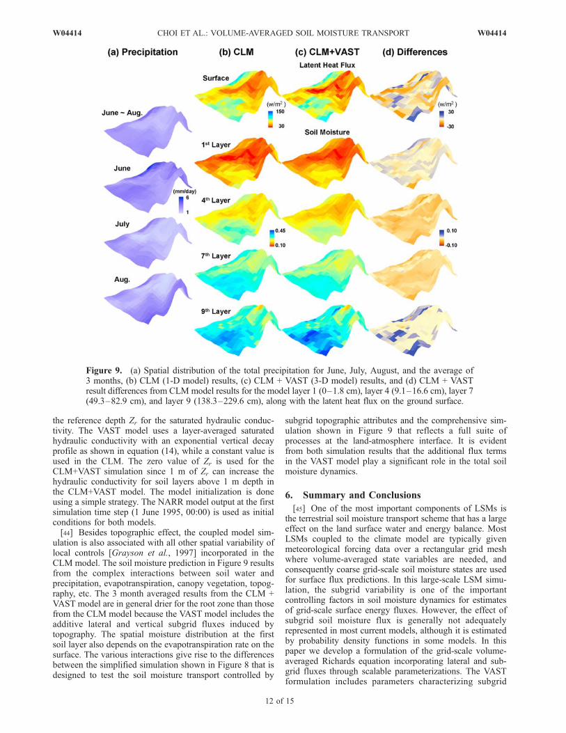
the reference depth Zr for the saturated hydraulic conduc-tivity. The VAST model uses a layer-averaged saturatedhydraulic conductivity with an exponential vertical decayprofile as shown in equation (14), while a constant value isused in the CLM. The zero value of Zr is used for theCLM+VAST simulation since 1 m of Zr can increase thehydraulic conductivity for soil layers above 1 m depth inthe CLM+VAST model. The model initialization is doneusing a simple strategy. The NARR model output at the firstsimulation time step (1 June 1995, 00:00) is used as initialconditions for both models.[44] Besides topographic effect, the coupled model sim-

ulation is also associated with all other spatial variability oflocal controls [Grayson et al., 1997] incorporated in theCLM model. The soil moisture prediction in Figure 9 resultsfrom the complex interactions between soil water andprecipitation, evapotranspiration, canopy vegetation, topog-raphy, etc. The 3 month averaged results from the CLM +VAST model are in general drier for the root zone than thosefrom the CLM model because the VAST model includes theadditive lateral and vertical subgrid fluxes induced bytopography. The spatial moisture distribution at the firstsoil layer also depends on the evapotranspiration rate on thesurface. The various interactions give rise to the differencesbetween the simplified simulation shown in Figure 8 that isdesigned to test the soil moisture transport controlled by

subgrid topographic attributes and the comprehensive sim-ulation shown in Figure 9 that reflects a full suite ofprocesses at the land-atmosphere interface. It is evidentfrom both simulation results that the additional flux termsin the VAST model play a significant role in the total soilmoisture dynamics.

6. Summary and Conclusions

[45] One of the most important components of LSMs isthe terrestrial soil moisture transport scheme that has a largeeffect on the land surface water and energy balance. MostLSMs coupled to the climate model are typically givenmeteorological forcing data over a rectangular grid meshwhere volume-averaged state variables are needed, andconsequently coarse grid-scale soil moisture states are usedfor surface flux predictions. In this large-scale LSM simu-lation, the subgrid variability is one of the importantcontrolling factors in soil moisture dynamics for estimatesof grid-scale surface energy fluxes. However, the effect ofsubgrid soil moisture flux is generally not adequatelyrepresented in most current models, although it is estimatedby probability density functions in some models. In thispaper we develop a formulation of the grid-scale volume-averaged Richards equation incorporating lateral and sub-grid fluxes through scalable parameterizations. The VASTformulation includes parameters characterizing subgrid

Figure 9. (a) Spatial distribution of the total precipitation for June, July, August, and the average of3 months, (b) CLM (1-D model) results, (c) CLM + VAST (3-D model) results, and (d) CLM + VASTresult differences from CLM model results for the model layer 1 (0–1.8 cm), layer 4 (9.1–16.6 cm), layer 7(49.3–82.9 cm), and layer 9 (138.3–229.6 cm), along with the latent heat flux on the ground surface.

12 of 15

W04414 CHOI ET AL.: VOLUME-AVERAGED SOIL MOISTURE TRANSPORT W04414

variability represented as scale-dependent functions withsecond order approximations. These parameterizations in-corporate statistical properties related to soil moisture vari-ability dependence on subgrid topographic attributes such asslopes and curvatures. We isolate subgrid topographic char-acteristics from other soil properties that may also affect soilmoisture dynamics, and perform closure parameterizationsfor topographic variability. Each soil property is assumed tobe constant within a grid volume and its variance and jointvariability for each other are ignored for lack of availabledata for closure of unknown covariance properties, which isthe same as the assumption that the meteorological forcingdata are constant over the computational grids. Theseparameterizations based on limited data sets serve to illus-trate the role of subgrid variability, and are not meant toserve as a universal model. Indeed, we hope that thisillustration will serve to catalyze the more consistent datacollection.[46] The relative contribution ratios incorporating these

parameters show that the variability terms are significantparticularly in drier soil moisture conditions. The subgridvariability effects are noticeable in both the vertical andlateral drainage components over most moisture conditions.The lateral drainage variability associated with the topo-graphic attributes is also sensitive to the computational gridscale. The subgrid flux induced by the topographic vari-ability can be significant in coarse grid models, and cannotbe neglected at even the fine grid spacing. It is also expectedthat the contribution of subgrid flux becomes less while the

lateral flux effects might become more to the total moisturedynamics as the model grid spacing decreases. Here we aimto illustrate through the relative contribution analysis thatthe subgrid flux plays a significant role in total soil moisture

dynamics. Ignoring subgrid variability terms can causesignificant model errors and consequential unrealistic modelparameters for calibration. The relative contribution analysisof the lateral to vertical terms is not performed in this paperas it is not analytically tractable. The next paper will alsopresent the lateral flow contribution at the current modelscale through the numerical simulation results.[47] The numerical solution of the VAST model can be

implemented using a time splitting scheme by separating thevertical and lateral components of the equation. An explicitmethod is used to solve the lateral flow after a fully implicitmethod for the vertical flow. The details of this scheme willbe presented in an upcoming paper. The example simulationresults illustrate that the subgrid and lateral flux contributionhas a significant impact on the total soil moisture dynamicsand the VAST model can be readily substituted for theexisting 1-D schemes in current LSMs.[48] A land surface model based on the VAST using

appropriate boundary conditions and sink terms, such asprecipitation, infiltration, vegetation effects, evapotranspi-ration and surface runoff, can improve the understanding ofsubgrid topographic impact on terrestrial hydrologic pro-cesses and predictability of the model.

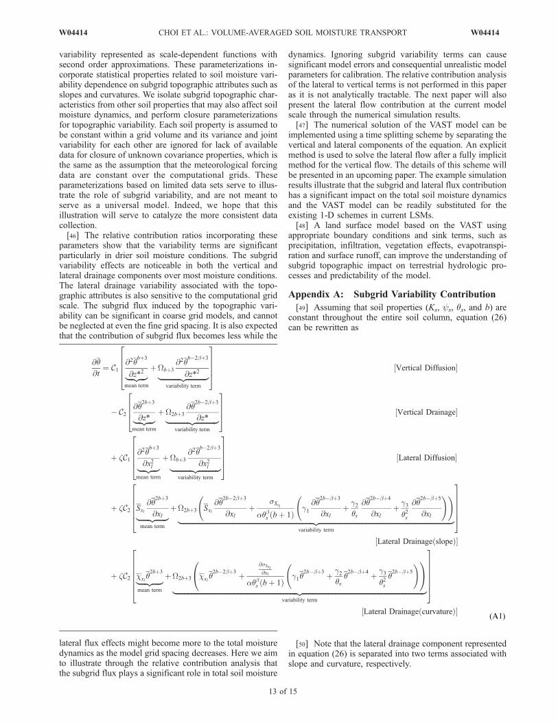
Appendix A: Subgrid Variability Contribution

[49] Assuming that soil properties (Ks, ys, qs, and b) areconstant throughout the entire soil column, equation (26)can be rewritten as

@q@t

¼ C1@2q

bþ3

@z*2|fflfflffl{zfflfflffl}mean term

þWbþ3

@2qb�2bþ3

@z*2|fflfflfflfflfflfflfflfflfflfflffl{zfflfflfflfflfflfflfflfflfflfflffl}variability term

26664

37775 Vertical Diffusion½ �

� C2@q

2bþ3

@z*|fflfflffl{zfflfflffl}mean term

þW2bþ3

@q2b�2bþ3

@z*|fflfflfflfflfflfflfflfflfflfflfflffl{zfflfflfflfflfflfflfflfflfflfflfflffl}variability term

2664

3775 Vertical Drainage½ �

þ zC1@2q

bþ3

@x2l|fflfflffl{zfflfflffl}mean term

þWbþ3

@2qb�2bþ3

@x2l|fflfflfflfflfflfflfflfflfflfflffl{zfflfflfflfflfflfflfflfflfflfflffl}variability term

26664

37775 Lateral Diffusion½ �

þ zC2 Sxl@q

2bþ3

@xl|fflfflfflfflfflffl{zfflfflfflfflfflffl}mean term

þW2bþ3 Sxl@q

2b�2bþ3

@xlþ

sSxl

aqbs bþ 1ð Þg1

@q2b�bþ3

@xlþ g2

qs

@q2b�bþ4

@xlþ g3

q2s

@q2b�bþ5

@xl

! !|fflfflfflfflfflfflfflfflfflfflfflfflfflfflfflfflfflfflfflfflfflfflfflfflfflfflfflfflfflfflfflfflfflfflfflfflfflfflfflfflfflfflfflfflfflfflfflfflfflfflfflfflfflfflfflfflfflfflfflfflfflfflfflfflfflfflfflfflfflfflfflfflfflfflfflfflffl{zfflfflfflfflfflfflfflfflfflfflfflfflfflfflfflfflfflfflfflfflfflfflfflfflfflfflfflfflfflfflfflfflfflfflfflfflfflfflfflfflfflfflfflfflfflfflfflfflfflfflfflfflfflfflfflfflfflfflfflfflfflfflfflfflfflfflfflfflfflfflfflfflfflfflfflfflffl}

variability term

266664

377775

Lateral Drainage slopeð Þ½ �

þ zC2 cxlq2bþ3|fflfflfflffl{zfflfflfflffl}

mean term

þW2bþ3 cxlq2b�2bþ3 þ

@sSxl

@xl

aqbs bþ 1ð Þg1q

2b�bþ3 þ g2qs

q2b�bþ4 þ g3

q2sq2b�bþ5

!0@

1A

|fflfflfflfflfflfflfflfflfflfflfflfflfflfflfflfflfflfflfflfflfflfflfflfflfflfflfflfflfflfflfflfflfflfflfflfflfflfflfflfflfflfflfflfflfflfflfflfflfflfflfflfflfflfflfflfflfflfflfflfflfflfflfflfflfflfflfflfflfflfflffl{zfflfflfflfflfflfflfflfflfflfflfflfflfflfflfflfflfflfflfflfflfflfflfflfflfflfflfflfflfflfflfflfflfflfflfflfflfflfflfflfflfflfflfflfflfflfflfflfflfflfflfflfflfflfflfflfflfflfflfflfflfflfflfflfflfflfflfflfflfflfflffl}variability term

2666664

3777775

Lateral Drainage curvatureð Þ½ �

[50] Note that the lateral drainage component representedin equation (26) is separated into two terms associated withslope and curvature, respectively.

(A1)

W04414 CHOI ET AL.: VOLUME-AVERAGED SOIL MOISTURE TRANSPORT

13 of 15

W04414

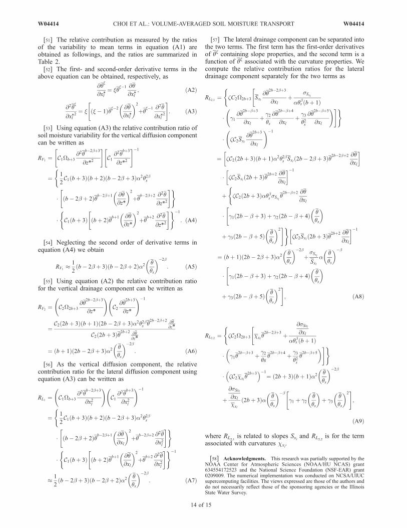
[51] The relative contribution as measured by the ratiosof the variability to mean terms in equation (A1) areobtained as followings, and the ratios are summarized inTable 2.[52] The first- and second-order derivative terms in the

above equation can be obtained, respectively, as

@qx

@xl*¼ xq

x�1 @q@xl*

; ðA2Þ

@2qx

@xl*2¼ x x � 1ð Þqx�2 @q

@xl*

� �2

þqx�1 @2q

@xl*2

" #: ðA3Þ

[53] Using equation (A3) the relative contribution ratio ofsoil moisture variability for the vertical diffusion componentcan be written as

RV1¼ C1�bþ3

@2�b�2�þ3

@z*2

" #C1

@2�bþ3

@z*2

" #�1

¼(1

2C1 bþ 3ð Þ bþ 2ð Þ b� 2� þ 3ð Þ�2�2�s

� b� 2� þ 2ð Þ�b�2�þ1 @�

@z*

� �2

þ�b�2�þ2 @2�

@z*2

" #)

� C1 bþ 3ð Þ bþ 2ð Þ�bþ1 @�

@z*

� �2

þ�bþ2 @2�

@z*2

" #( )�1

: ðA4Þ

[54] Neglecting the second order of derivative terms inequation (A4) we obtain

RV1 1

2b� 2b þ 3ð Þ b� 2b þ 2ð Þa2 q

qs

� ��2b

: ðA5Þ

[55] Using equation (A2) the relative contribution ratiofor the vertical drainage component can be written as

RV2¼ C2�2bþ3

@�2b�2�þ3

@z*

!C2

@�2bþ3

@z*

!�1

¼C2 2bþ 3ð Þ bþ 1ð Þ 2b� 2� þ 3ð Þ�2�2�s �

2b�2�þ2 @�@z*

C2 2bþ 3ð Þ�2bþ2 @�@z*

¼ bþ 1ð Þ 2b� 2� þ 3ð Þ�2 �

�s

� ��2�

: ðA6Þ

[56] As the vertical diffusion component, the relativecontribution ratio for the lateral diffusion component usingequation (A3) can be written as

RL1 ¼ C1�bþ3

@2�b�2�þ3

@x2l

!C1

@2�bþ3

@x2l

!�1

¼(1

2C1 bþ 3ð Þ bþ 2ð Þ b� 2� þ 3ð Þ�2�2�s

� b� 2� þ 2ð Þ�b�2�þ1 @�

@xl

� �2

þ�b�2�þ2 @2�

@x2l

" #)

� C1 bþ 3ð Þ bþ 2ð Þ�bþ1 @�

@xl

� �2

þ�bþ2 @2�

@x2l

" #( )�1

1

2b� 2� þ 3ð Þ b� 2� þ 2ð Þ�2 �

�s

� ��2�

: ðA7Þ

[57] The lateral drainage component can be separated intothe two terms. The first term has the first-order derivativesof qx containing slope properties, and the second term is afunction of qx associated with the curvature properties. Wecompute the relative contribution ratios for the lateraldrainage component separately for the two terms as

RL2;1 ¼(�C2�2bþ3

"Sxl

@�2b�2�þ3

@xlþ

Sxl

���s bþ 1ð Þ

� 1@�

2b��þ3

@xlþ 2

�s

@�2b��þ4

@xlþ 3

�2s

@�2b��þ5

@xl

!#)

� �C2Sxl

@�2bþ3

@xl

!�1

¼ �C2 2bþ 3ð Þ bþ 1ð Þ�2�2�s Sxl 2b� 2� þ 3ð Þ�2b�2�þ2 @�

@xl

� �

� �C2Sxl 2bþ 3ð Þ�2bþ2 @�

@xl

� ��1

þ(�C2 2bþ 3ð Þ���s Sxl

�2b��þ2 @�

@xl

�"1 2b� � þ 3ð Þ þ 2 2b� � þ 4ð Þ �

�s

� �

þ 3 2b� � þ 5ð Þ �

�s

� �2#)

�C2Sxl 2bþ 3ð Þ�2bþ2 @�

@xl

� ��1

¼ bþ 1ð Þ 2b� 2� þ 3ð Þ�2 �

�s

� ��2�

þSxl

Sxl�

�

�s

� ���

�"1 2b� � þ 3ð Þ þ 2 2b� � þ 4ð Þ �

�s

� �

þ 3 2b� � þ 5ð Þ �

�s

� �2#; ðA8Þ

RL2;2 ¼(�C2�2bþ3

"�xl

�2b�2�þ3 þ

@Sxl@xl

���s bþ 1ð Þ

� 1�2b��þ3 þ 2

�s�2b��þ4 þ 3

�2s�2b��þ5

� �#)

� �C2�xl�2bþ3

� �1

¼ 2bþ 3ð Þ bþ 1ð Þ�2 �

�s

� ��2�

þ

@Sxl@xl�xl

2bþ 3ð Þ� �

�s

� ���

1 þ 2�

�s

� �þ 3

�

�s

� �2" #

;

ðA9Þ

where RL2,1is related to slopes Sxl and RL2,2

is for the termassociated with curvatures cxl

.

[58] Acknowledgments. This research was partially supported by theNOAA Center for Atmospheric Sciences (NOAA/HU NCAS) grant634554172523 and the National Science Foundation (NSF-EAR) grant0209009. The numerical implementation was conducted on NCSA/UIUCsupercomputing facilities. The views expressed are those of the authors anddo not necessarily reflect those of the sponsoring agencies or the IllinoisState Water Survey.

14 of 15

W04414 CHOI ET AL.: VOLUME-AVERAGED SOIL MOISTURE TRANSPORT W04414

ReferencesBeven, K. J., and M. J. Kirkby (1979), A physically based variable con-tributing area model of basin hydrology, Hydrol. Sci. Bull., 24(1), 43–69.

Boone, A., and P. Wetzel (1996), Issues related to low resolution modelingof soil moisture: Experience with the PLACE model, Global Planet.Change, 13, 161–181.

Brooks, R. H., and A. T. Corey (1964), Hydraulic properties in porousmedia, Hydrol. Pap. 3, 27 pp., Colo. State Univ., Fort Collins.

Chen, J., and P. Kumar (2001), Topographic influence on the seasonal andinter-annual variation of water and energy balance of basins in NorthAmerica, J. Clim., 14(9), 1989–2014.

Chen, J., and P. Kumar (2002), Role of terrestrial hydrologic memory inmodulating ENSO impacts in North America, J. Clim., 15(24), 3569–3585.

Chen, J., and P. Kumar (2004), A modeling study of the ENSO influence onthe terrestrial energy profile over North America, J. Clim., 17(8), 1657–1670.

Clapp, R. B., and G. M. Hornberger (1978), Empirical equations for somesoil hydraulic properties, Water Resour. Res., 14, 601–604.

Cosby, B. J., G. M. Hornberger, R. B. Clapp, and T. R. Ginn (1984), Astatistical exploration of the relationships of soil moisture characteristicsto the physical properties of soils, Water Resour. Res., 20, 682–690.

Dai, Y., et al. (2001), The Common land model (CLM): Technical docu-mentation and user’s guide, Ga. Inst. of Technol., Atlanta. (Available athttp://climate.eas.gatech.edu/dickinson/)

Dai, Y., et al. (2003), The common land model, Bull. Am. Meteorol. Soc.,84, 1013–1023.

Famiglietti, J. S., J. A. Devereaux, C. Laymon, T. Tsegaye, P. R. Houser,T. J. Jackson, S. T. Graham, M. Rodell, and P. J. van Oevelen (1999),Ground-based investigation of spatial-temporal soil moisture variabilitywithin remote sensing footprints during SGP97, Water Resour. Res., 35,1839–1851.

Freeze, R. A., and J. A. Cherry (1979), Groundwater, Prentice-Hall, UpperSaddle River, N. J.

Gochis, D. J., G. Bonan, E. Brandes, F. Chen, M. Ek, D. Lenschow, M. M.LeMone, R. Rasmussen, and T. T. Warner (2004), A ten-year vision forresearch on terrestrial-atmospheric interactions: Advancing coupled land-

atmosphere prediction, report, Consortium of Univ. for the Adv. ofHydrol. Sci., Washington, D. C. (Available at http://www.cuahsi.org/cyberseminars/Gochis-20041201-paper.pdf)

Grayson, R. B., A. W. Western, F. H. S. Chiew, and G. Bloschl (1997),Preferred states in spatial soil moisture patterns: Local and nonlocalcontrols, Water Resour. Res., 33, 2897–2908.

Koster, R. D., M. J. Suarez, A. Ducharne, M. Stieglitz, and P. Kumar(2000), A catchment-based approach to modeling land surface processesin a GCM: 1. Model structure, J. Geophys. Res., 105, 24,809–24,822.

Kumar, P. (2004), Layer averaged Richard’s equation with lateral flow, Adv.Water Resour., 27(5), 521–531.

Liang, X.-Z., L. Li, K. E. Kunkel, M. Ting, and J. X. L. Wang (2004),Regional climate model simulation of U.S. precipitation during 1982–2002. Part 1: Annual cycle, J. Clim., 17, 2528–3510.

Liang, X.-Z., H. I. Choi, K. E. Kunkel, Y. Dai, E. Joseph, J. X. L. Wang,and P. Kumar (2005), Surface boundary conditions for mesoscale regio-nal climate models, Earth Inter., 9, Paper 18, 28 pp.

Montaldo, N., and J. D. Albertson (2003), Temporal dynamics of soil moist-ure variability at the landscape scale: 2. Implications for land surfacemodels, Water Resour. Res., 39(10), 1275, doi:10.1029/2002WR001618.

Western, A. W., R. B. Grayson, G. Bloschl, G. R. Willgoose, and T. A.McMahon (1999), Observed spatial organization of soil moisture and itsrelation to terrain indices, Water Resour. Res., 35, 797–810.

Wetzel, P. J., and A. Boone (1995), A parameterization for land-atmosphere-cloud exchange (PLACE): Documentation of a detailed pro-cess model of the partly cloudy boundary layer over heterogeneous land,J. Clim., 8, 1810–1837.

����������������������������H. I. Choi and P. Kumar, Environmental Hydrology and Hydraulic

Engineering, Department of Civil and Environmental Engineering,University of Illinois at Urbana-Champaign, 205 North Mathews Avenue,Urbana, IL 61801, USA. (hichoi@uiuc.edu; kumar1@uiuc.edu)

X.-Z. Liang, Center for Atmospheric Science, Illinois State WaterSurvey, University of Illinois at Urbana-Champaign, 2204 Griffith Drive,Champaign, IL 61820, USA. (xliang@uiuc.edu)

W04414 CHOI ET AL.: VOLUME-AVERAGED SOIL MOISTURE TRANSPORT

15 of 15

W04414