Geophysical Research Letters

RESEARCH LETTER10.1002/2013GL059114

Key Points:• Geometric attributes of topographic

depressions follow power lawdistributions

• Scaling laws have implications for thetransport of water and material fluxes

• Short distance among depressionscan affect hydrologic connectivity

Supporting Information:• Readme• Table S1

Correspondence to:P. Kumar,kumar1@illinois.edu

Citation:Le, P. V. V., and P. Kumar (2014),Power law scaling of topographicdepressions and their hydrologicconnectivity, Geophys. Res. Lett., 41,doi:10.1002/2013GL059114.

Received 27 DEC 2013

Accepted 7 FEB 2014

Accepted article online 14 FEB 2014

Power law scaling of topographic depressionsand their hydrologic connectivityPhong V. V. Le1 and Praveen Kumar1,2

1Department of Civil and Environmental Engineering, University of Illinois at Urbana-Champaign, Urbana, Illinois, USA,2Department of Atmospheric Sciences, University of Illinois at Urbana-Champaign, Urbana, Illinois, USA

Abstract Topographic depressions, areas of no lateral surface flow, are ubiquitous characteristics ofthe land surface that control many ecosystem and biogeochemical processes. High density ofdepressions increases the surface storage capacity, whereas lower depression density increases runoff, thusinfluencing soil moisture states, hydrologic connectivity, and the climate-soil-vegetation interactions. Withthe widespread availability of high-resolution lidar-based digital elevation model (lDEM) data, it is nowpossible to identify and characterize the structure of the spatial distribution of topographic depressionsfor incorporation in ecohydrologic and biogeochemical studies. Here we use lDEM data to document theprevalence and patterns of topographic depressions across five different landscapes in the United Statesand quantitatively characterize the probability distribution of attributes, such as surface area, storagevolume, and the distance to the nearest neighbor. Through the use of a depression identification algorithm,we show that these probability distributions of attributes follow scaling laws indicative of a structure inwhich a large fraction of land surface areas can consist of high number of topographic depressions of allsizes and can account for 4 to 21 mm of depression storage. This implies that the impacts of small-scaletopographic depressions in the landscapes on the redistribution of material fluxes, evaporation, andhydrologic connectivity are quite significant.

1. Introduction

Several hydrological and ecological studies have indicated that depressions arising from microtopo-graphic variability can have significant effects on streamflow generation [Dunne et al., 1991; Frei et al., 2010;Thompson et al., 2010; Loos and Elsenbeer, 2011], soil moisture dynamics [Simmons et al., 2011], and veg-etation patterns [Moser et al., 2007; Scanlon et al., 2007; McGrath et al., 2012]. Based on studies involvingsynthetic microtopographic features, it has been suggested that ignoring these features may lead to signif-icant biases in the prediction of hydrological partitioning of rainfall into infiltration and runoff [Dunne et al.,1991; Thompson et al., 2010]. However, existing methods of topographic analyses based on lower resolutiondigital elevation models (DEMs) have relied on “depression filling” algorithms [O’Callaghan and Mark, 1984;Planchon and Darboux, 2002] to focus on stream network extraction and analyses and have not focusedon the attributes of the topographic depressions themselves. The increasing availability of high-resolution(∼1–3 m grid spacing) topographic data from light detection and ranging (lidar) data has offered newopportunities for broader exploration of landscape structures at fine scales [Lefsky et al., 2002; Schwarz, 2010;Ussyshkin and Theriault, 2011] and new algorithms have been developed for automatic extraction of geo-morphic features on both natural and human-modified landscapes [Lashermes et al., 2007; Vianello et al.,2009; Passalacqua et al., 2010, 2012; Li et al., 2011]. In the present work we use a depression identificationmodel [Chu et al., 2010; Shaw et al., 2012; Chu et al., 2013] to analyze lDEM data across five different land-scapes and quantitatively characterize geometric attributes of topographic depression such as surface area,storage volume, and distance to the nearest neighbor, which are critical to understanding and linking land-scape patterns and processes. This study for the first time presents the scaling relationships for attributes oftopographic depression obtained from lDEM data.

2. Methods2.1. Topographic Depression IdentificationTopographic depression identification (TDI) is accomplished using conceptual framework recently published[Chu et al., 2010; Shaw et al., 2012; Chu et al., 2013] but with performance improvement achieved through

LE AND KUMAR ©2014. American Geophysical Union. All Rights Reserved. 1

Geophysical Research Letters 10.1002/2013GL059114

Groundwater

A

hmax

Lowest point

RunoffThresholdpoint

(b)

(d)(c)

Transient pond

Filling - Merging Draining - Splitting

Level 1

1leveL2leveL

Level 2

Depressions

Nor

thin

g (m

)

Easting (m)

(e)

Vadose zone

Transient pond

Transient pond

infiltration

evaporation

X

Y

(a)

Figure 1. Schematic of topographic depression identification (TDI) processes on land surface using lidar data (adapted from Chu et al. [2010], Shaw et al. [2012],and Chu et al. [2013]). (a) An illustration of land surface with depressions (red circles). (b) Definition of geometric attributes characterizing topographic depres-sions. Rainfall and runoff fill water in depressions to create transient ponds on the land surface. Ponds are subject to infiltration and evapotranspiration that drainthe water. (c and d) Illustration of the role of different levels of depressions through fill-merging processes due to rainfall and runoff, and draining-splitting pro-cesses due to evaporation and infiltration. (e) An example of shaded relief map of lidar data in Bird’s Point-New Madrid Floodway with identified topographicdepressions (red polygons) at level 4.

implementation of a new algorithm that uses connected component labeling [Rosenfeld and Pfaltz, 1966]and morphological approach [Serra, 1983; Haralick et al., 1987; Giardina and Dougherty, 1988]. The TDI mod-els use the D8 algorithm proposed by O’Callaghan and Mark [1984] for identifying depressions [Chu et al.,2010; Shaw et al., 2012; Chu et al., 2013]. This approach uses flow directions, assigned from each cell to oneof its eight neighbors with the steepest downward slope, to identify the lowest elevation points (local ele-vation minima) of each depression. From these minima, local search algorithms are then implemented toidentify depression cells and the elevation thresholds for overflow for every depression on the land surface[Chu et al., 2010]. Thresholds are the highest points (local elevation maxima) of depressions through whichponded water in the depressions spills to surrounding areas (Figure 1). Depressions are assumed to mergeor split as water level reaches the common elevation thresholds from incoming rainfall and runoff, or outgo-ing infiltration and evaporation, respectively, which alter the “level” of the depressions. Following Chu et al.[2010], we use the following notation for delineating different levels of depression. The simplest depressionwith a single local minima and a spillover threshold defined by a single local maxima is identified as level 1(l1). Depressions of higher level (lm+1) are created when two depressions at level lm and ln merge (under theassumption of more water accumulation and lm > ln) (see Figure 1).

Data of lDEM at 1 m and 1.5 m resolutions, depending on study sites, are used as the inputs for the enhancedTDI model. The lDEM data for five locations (with the same dimension of 4 km × 4 km) across the UnitedStates, representing different landscapes (see Table 1) were obtained from the OpenTopography project (seehttp://www.opentopography.org) and the U.S. Army Corps of Engineers. In dense vegetation cover areas,lidar data collected during leaf-off periods is chosen to avoid the impacts of vegetation cover. These datasets contain missing data in the range 0–2% of the grid points, depending on the sites. Image inpaintinginterpolation [Bertalmio et al., 2000] and simple nearest-neighbor interpolation techniques are used for gapfilling and correction of missing data. We also assume that topographic features are fixed and no erosion ordeposition occurs in short timescales. The analysis using the TDI approach results in a spatial grid for each

LE AND KUMAR ©2014. American Geophysical Union. All Rights Reserved. 2

Geophysical Research Letters 10.1002/2013GL059114

Table 1. Characteristics of Different Study Sites in the United Statesa

Latitude/ Accuracyz n 𝛾 S̄aSite Name Longitude (cm) (-) (-) (mm) Landscape

Christina River Basin, PA 39.49◦N, 3–5 8310 0.06 20.4 Natural75.51◦W

Iowa River Floodplain, IA 41.41◦N, 3–10 2447 0.04 4.3 Human modified91.58◦W

Bird’s Point-New Madrid 36.97◦N, 10–15 12069 0.15 15.9 Human modified(BPNM) Floodway, MO 89.16◦WOhywee River Basin, OR 43.21◦N, 5–15 4214 0.02 7.1 Natural

117.55◦WMojave Desert, CA 34.73◦N, 5–15 3582 0.02 4.9 Desert

115.65◦WaAll sites are 4 km × 4 km in area. Accuracyz represents the vertical accuracy of lidar data on

each site, n represents the number of depressions on each site, 𝛾 represents the density of depres-sions on each site, and S̄a represents the average abstraction in each site.

level of depression, with each grid point identified as a depression or not at that level (Figure 1e).for thecomputations (see supporting information)

2.2. Topographic Depression CharacterizationGeometric attributes of the depression are estimated from the TDI model’s outputs. The surface area of anydepression represents the largest surface area of ponded water assuming that water levels are at the thresh-old elevation (Figure 1b). The surface area of the kth depression at level l, say A(l)

k [L2], is the sum of the areasof all individual grid cells within that depression. Similarly, the storage volume of topographic depressionsis the corresponding maximum storage of ponded water assuming water level is at the threshold elevation.The storage volume of the kth depression at level l, denoted as V (l)

k [L3], is given by

V (l)k =

mk∑i=1

(z(l)k,t − z(l)k,i

)ΔxΔy (1)

where mk is the number of cells, z(l)k,t[L] is the elevation of the threshold and z(l)k,i[L] is the elevation of ithcell, respectively, in the kth depression at level l. Δx[L] and Δy[L] are the uniform horizontal resolution ofthe lDEM data (Δx = Δy = 1 m in our data, except for Bird’s Point New Madrid (BPNM) Floodway whereΔx = Δy = 1.5 m). The maximum (or deepest) depth of a depression at level l, denoted as h(l)

k,max[L], is thedifference in elevation between the lowest cell and the threshold (Figure 1b), i.e.,

h(l)k,max = max

1≤i≤mk

(z(l)k,t − z(l)k,i

)(2)

To avoid errors limited by the achievable accuracy of lidar data, we only considered depressions whose max-imum depth is greater than or equal to 10 cm. The vertical accuracy of lidar data at each site is presented inTable 1. The average depth of the kth depression at level l, denoted as h̄(l)

k [L], is given by

h̄(l)k = V (l)

k

/A(l)

k (3)

Depression storage, Sa[L], resulting from maximum depression storage volume (at the highest level lmax) onland surface with respect to rainfall of depth P[L], is calculated as:

Sa =

(n∑

k=1

min(h̄(lmax)k , P) × A(h,lmax)

k

)/Atot (4)

where Atot[L2] is the total area of the domain of study, and n is the number of depressions at level lmax

found in the domain. The distance between two topographic depressions are defined as the Euclidean dis-tance between their lowest cells. The distance to the nearest neighbor (shortest distance, D(l)[L]) of everydepression at different levels are also calculated for cluster size analysis.

LE AND KUMAR ©2014. American Geophysical Union. All Rights Reserved. 3

Geophysical Research Letters 10.1002/2013GL059114

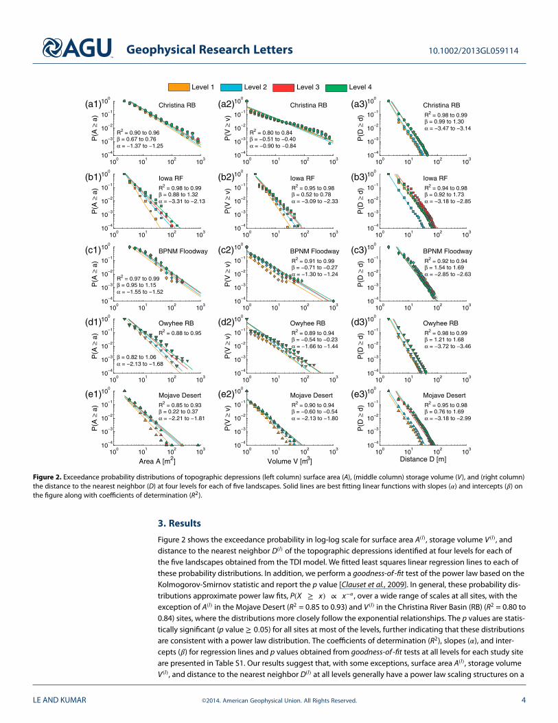
Figure 2. Exceedance probability distributions of topographic depressions (left column) surface area (A), (middle column) storage volume (V), and (right column)the distance to the nearest neighbor (D) at four levels for each of five landscapes. Solid lines are best fitting linear functions with slopes (𝛼) and intercepts (𝛽) onthe figure along with coefficients of determination (R2).

3. Results

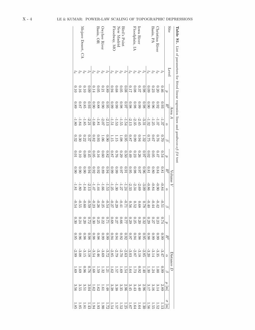
Figure 2 shows the exceedance probability in log-log scale for surface area A(l), storage volume V (l), anddistance to the nearest neighbor D(l) of the topographic depressions identified at four levels for each ofthe five landscapes obtained from the TDI model. We fitted least squares linear regression lines to each ofthese probability distributions. In addition, we perform a goodness-of -fit test of the power law based on theKolmogorov-Smirnov statistic and report the p value [Clauset et al., 2009]. In general, these probability dis-tributions approximate power law fits, P(X ≥ x) ∝ x−𝛼 , over a wide range of scales at all sites, with theexception of A(l) in the Mojave Desert (R2 = 0.85 to 0.93) and V (l) in the Christina River Basin (RB) (R2 = 0.80 to0.84) sites, where the distributions more closely follow the exponential relationships. The p values are statis-tically significant (p value ≥ 0.05) for all sites at most of the levels, further indicating that these distributionsare consistent with a power law distribution. The coefficients of determination (R2), slopes (𝛼), and inter-cepts (𝛽) for regression lines and p values obtained from goodness-of -fit tests at all levels for each study siteare presented in Table S1. Our results suggest that, with some exceptions, surface area A(l), storage volumeV (l), and distance to the nearest neighbor D(l) at all levels generally have a power law scaling structures on a

LE AND KUMAR ©2014. American Geophysical Union. All Rights Reserved. 4

Geophysical Research Letters 10.1002/2013GL059114

0 5 10 15 20 25 30 350

5

10

15

20

25

Rainfall depth [mm]

Sa

[mm

]

Christina RBIowa RFBPNM FloodwayOwyhee RBMojave Desert

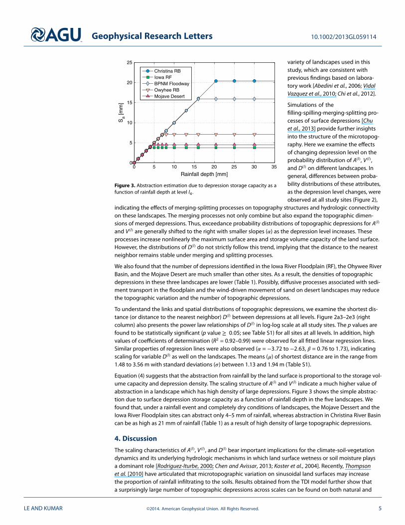
Figure 3. Abstraction estimation due to depression storage capacity as afunction of rainfall depth at level l4.

variety of landscapes used in thisstudy, which are consistent withprevious findings based on labora-tory work [Abedini et al., 2006; VidalVazquez et al., 2010; Chi et al., 2012].

Simulations of thefilling-spilling-merging-splitting pro-cesses of surface depressions [Chuet al., 2013] provide further insightsinto the structure of the microtopog-raphy. Here we examine the effectsof changing depression level on theprobability distribution of A(l), V (l),and D(l) on different landscapes. Ingeneral, differences between proba-bility distributions of these attributes,as the depression level changes, wereobserved at all study sites (Figure 2),

indicating the effects of merging-splitting processes on topography structures and hydrologic connectivityon these landscapes. The merging processes not only combine but also expand the topographic dimen-sions of merged depressions. Thus, exceedance probability distributions of topographic depressions for A(l)

and V (l) are generally shifted to the right with smaller slopes (𝛼) as the depression level increases. Theseprocesses increase nonlinearly the maximum surface area and storage volume capacity of the land surface.However, the distributions of D(l) do not strictly follow this trend, implying that the distance to the nearestneighbor remains stable under merging and splitting processes.

We also found that the number of depressions identified in the Iowa River Floodplain (RF), the Ohywee RiverBasin, and the Mojave Desert are much smaller than other sites. As a result, the densities of topographicdepressions in these three landscapes are lower (Table 1). Possibly, diffusive processes associated with sedi-ment transport in the floodplain and the wind-driven movement of sand on desert landscapes may reducethe topographic variation and the number of topographic depressions.

To understand the links and spatial distributions of topographic depressions, we examine the shortest dis-tance (or distance to the nearest neighbor) D(l) between depressions at all levels. Figure 2a3–2e3 (rightcolumn) also presents the power law relationships of D(l) in log-log scale at all study sites. The p values arefound to be statistically significant (p value ≥ 0.05; see Table S1) for all sites at all levels. In addition, highvalues of coefficients of determination (R2 = 0.92–0.99) were observed for all fitted linear regression lines.Similar properties of regression lines were also observed (𝛼 = −3.72 to −2.63, 𝛽 = 0.76 to 1.73), indicatingscaling for variable D(l) as well on the landscapes. The means (𝜇) of shortest distance are in the range from1.48 to 3.56 m with standard deviations (𝜎) between 1.13 and 1.94 m (Table S1).

Equation (4) suggests that the abstraction from rainfall by the land surface is proportional to the storage vol-ume capacity and depression density. The scaling structure of A(l) and V (l) indicate a much higher value ofabstraction in a landscape which has high density of large depressions. Figure 3 shows the simple abstrac-tion due to surface depression storage capacity as a function of rainfall depth in the five landscapes. Wefound that, under a rainfall event and completely dry conditions of landscapes, the Mojave Dessert and theIowa River Floodplain sites can abstract only 4–5 mm of rainfall, whereas abstraction in Christina River Basincan be as high as 21 mm of rainfall (Table 1) as a result of high density of large topographic depressions.

4. Discussion

The scaling characteristics of A(l), V (l), and D(l) bear important implications for the climate-soil-vegetationdynamics and its underlying hydrologic mechanisms in which land surface wetness or soil moisture playsa dominant role [Rodriguez-Iturbe, 2000; Chen and Avissar, 2013; Koster et al., 2004]. Recently, Thompsonet al. [2010] have articulated that microtopographic variation on sinusoidal land surfaces may increasethe proportion of rainfall infiltrating to the soils. Results obtained from the TDI model further show thata surprisingly large number of topographic depressions across scales can be found on both natural and

LE AND KUMAR ©2014. American Geophysical Union. All Rights Reserved. 5

Geophysical Research Letters 10.1002/2013GL059114

human-modified landscapes, thus increasing surface storage abstraction. In addition to canopy intercep-tion loss (up to 16 mm) [Carlyle-Moses and Gash, 2011], this abstraction is larger in areas which have highmicrotopographic variability (Figure 3), implying that hydrological partitioning of rainfall into runoff can befurther reduced significantly by surface depressions. These increases are more important in water-controlledecosystems where water may be a limiting factor or in regions where small intensity rainstorm events dom-inate the precipitation patterns. Moreover, low negative topographic scaling factors of A(l) (𝛼 = −1.25to −3.31) and V (l) (𝛼 = −0.84 to −3.09) indicate that smaller-scale depressions on landscapes, which areoften neglected in previous studies, tend to produce larger total water storage volume and open surfacearea. This suggests that the impacts of small-scale topographic depressions in the landscapes on evapo-ration and the redistribution of surface energy fluxes are quite significant, and a microtopographic factorshould be included along with local topographic features, e.g., slope and aspect that influence surfaceenergy and water balances [Vico and Porporato, 2009] and other processes in the study of climate-soil-vegetation interactions.

The distance to the nearest neighbor D(l) exhibits scaling characteristics, which may affect hydrologic con-nectivity that in turn controls the transport of water and other material fluxes on the landscape [Pringle,2001]. Generally, topographic depressions are localized, collecting and storing water from specific contribut-ing areas. As water elevations reach the overflow thresholds, surface runoff links topographic depressionsto the channel system or other depressions, thus increasing hydrologic connectivity. The relatively highnumber of small-scale topographic depressions on the land surface imply that, in dry condition, hydro-logic connectivity is lower than previously thought. However, the universal power law distributions of D(l)

indicate that whereas most topographic depressions on land surface are generally linked by short dis-tances, a few link to the neighbors by long distances. This pattern of transient water bodies may quicklyincrease hydrologic connectivity as the system becomes wet. Nevertheless, hydrologic connectivity is alsolargely controlled by channel and subsurface systems. Comprehensive theory that links depressions to thesesystems using networks must therefore be investigated with caution.

5. Conclusion

We have applied a depression identification model, using lDEM data, to quantitatively characterize the geo-metric attributes of topographic depressions on natural and human-modified landscapes. These attributes,including surface area A(l), storage volume V (l), and distance to the nearest-neighbor D(l), have been shownto follow the power law distributions in their spatial variations over a broad range of scales in five dif-ferent landscapes in the United States. We showed that a large fraction of the land surface can have arelatively high number of topographic depressions across scales. The scaling relationships of these attributesalso suggest that small-scale topographic depressions may have significant impacts on the interactionsbetween climate, soil, vegetation, and the underlying hydrologic mechanisms. Moreover, the results demon-strated that surface topographic depressions are generally linked by short distances, implying impacts onhydrologic connectivity. Understanding how the scaling characteristics of topographic depressions on land-scapes affect land-atmosphere interaction, hydrologic connectivity, and land-surface processes is of criticalimportance and a challenge for ecohydrological sciences. This study extends our understanding of scalingcharacteristics of landscapes such as river networks [Rodriguez-Iturbe and Rinaldo, 1997; Rinaldo et al., 1998]and topography as fractal surfaces [Dodds and Rothman, 2000; Gagnon et al., 2006; Turcotte, 1997].

ReferencesAbedini, M., W. Dickinson, and R. Rudra (2006), On depressional storages: The effect of DEM spatial resolution, J. Hydrol., 318(1-4),

138–150.Bertalmio, M., G. Sapiro, V. Caselles, and C. Ballester (2000), Image inpainting, in Proceedings of the 27th Annual Conference on Com-

puter Graphics and Interactive Techniques, SIGGRAPH ’00, pp. 417–424, ACM Press/Addison-Wesley Publishing Co., New York,doi:10.1145/344779.344972.

Carlyle-Moses, D., and J. Gash (2011), Rainfall interception loss by forest canopies, in Forest Hydrology and Biogeochemistry, EcologicalStudies, vol. 216, edited by D. F. Levia, D. Carlyle-Moses, and T. Tanaka, pp. 407–423, Springer, Houten, Netherlands.

Chen, F., and R. Avissar (2013), Impact of land-surface moisture variability on local shallow convective cumulus and precipitation inlarge-scale models, J. Appl. Meteorol., 33(12), 1382–1401.

Chi, Y., J. Yang, D. Bogart, and X. Chu (2012), Fractal analysis of surface microtopography and its application in understanding hydrologicprocesses, Trans. ASABE, 55(5), 1781–1792.

Chu, X., J. Zhang, Y. Chi, and J. Yang (2010), An improved method for watershed delineation and computation of surface depressionstorage, in Watershed Management 2010: Innovations in Watershed Management Under Land Use and Climate Change, chap. 99, editedby K. W. Potter and D. K. Frevert, pp. 1113–1122, American Society of Civil Engineers, Reston, Va., doi:10.1061/41143(394)100.

AcknowledgmentsWe gratefully acknowledge NSFRAPID grant EAR 11-40198, NSF CBET12-09402, and NSF EAR 13-31906.The USACE provided the processedlidar 2011 DEM for BPNM through aMemorandum of Understanding withUniversity of Illinois. Other lidar datasets are based on services providedby the OpenTopography Facility withsupport under NSF awards 0930731and 0930643. Support from Universityof Illinois Research Board grant(11131), Innovation grant from theDepartment of Civil and EnvironmentalEngineering, and Fellowship from theComputational Science and Engineer-ing Program at University of Illinois arealso gratefully acknowledged.

The Editor thanks two anonymousreviewers for their assistance inevaluating this paper.

LE AND KUMAR ©2014. American Geophysical Union. All Rights Reserved. 6

Geophysical Research Letters 10.1002/2013GL059114

Chu, X., J. Yang, Y. Chi, and J. Zhang (2013), Dynamic puddle delineation and modeling of puddle-to-puddlefilling-spilling-merging-splitting overland flow processes, Water Resour. Res., 49, 3825–3829, doi:10.1002/wrcr.20286.

Clauset, A., C. Shalizi, and M. Newman (2009), Power-law distributions in empirical data, SIAM Rev., 51(4), 661–703,doi:10.1137/070710111.

Dodds, P. S., and D. H. Rothman (2000), Scaling, universality, and geomorphology, Annu. Rev. Earth Planet. Sci., 28(1), 571–610.Dunne, T., W. Zhang, and B. F. Aubry (1991), Effects of rainfall, vegetation, and microtopography on infiltration and runoff, Water Resour.

Res., 27(9), 2271–2285, doi:10.1029/91WR01585.Frei, S., G. Lischeid, and J. Fleckenstein (2010), Effects of micro-topography on surface-subsurface exchange and runoff generation in a

virtual riparian wetland—A modeling study, Adv. Water Resour., 33(11), 1388–1401, doi:10.1016/j.advwatres.2010.07.006.Gagnon, J.-S., S. Lovejoy, and D. Schertzer (2006), Multifractal Earth topography, Nonlinear Processes Geophys., 13(5), 541–570,

doi:10.5194/npg-13-541-2006.Giardina, C. R., and E. R. Dougherty (1988), Morphological Methods in Image and Signal Processing, Prentice-Hall, Inc., Upper Saddle River,

N. J.Haralick, R., S. R. Sternberg, and X. Zhuang (1987), Image analysis using mathematical morphology, IEEE Trans. Pattern Anal. Mach. Intell.,

PAMI-9(4), 532–550, doi:10.1109/TPAMI.1987.4767941.Koster, R. D., et al. (2004), Regions of strong coupling between soil moisture and precipitation, Science, 305(5687), 1138–1140,

doi:10.1126/science.1100217.Lashermes, B., E. Foufoula-Georgiou, and W. E. Dietrich (2007), Channel network extraction from high resolution topography using

wavelets, Geophys. Res. Lett., 34, L23S04, doi:10.1029/2007GL031140.Lefsky, M. A., W. B. Cohen, G. G. Parker, and D. J. Harding (2002), Lidar remote sensing for ecosystem studies, BioScience, 52(1), 19–30.Li, S., R. MacMillan, D. A. Lobb, B. G. McConkey, A. Moulin, and W. R. Fraser (2011), Lidar DEM error analyses and topographic

depression identification in a hummocky landscape in the prairie region of Canada, Geomorphology, 129(3-4), 263–275,doi:10.1016/j.geomorph.2011.02.020.

Loos, M., and H. Elsenbeer (2011), Topographic controls on overland flow generation in a forest—An ensemble tree approach, J. Hydrol.,409(1-2), 94–103, doi:10.1016/j.jhydrol.2011.08.002.

McGrath, G. S., K. Paik, and C. Hinz (2012), Microtopography alters self-organized vegetation patterns in water-limited ecosystems, J.Geophys. Res., 117, G03021, doi:10.1029/2011JG001870.

Moser, K., C. Ahn, and G. Noe (2007), Characterization of microtopography and its influence on vegetation patterns in created wetlands,Wetlands, 27(4), 1081–1097.

O’Callaghan, J. F., and D. M. Mark (1984), The extraction of drainage networks from digital elevation data, Comput. Vision Graphics ImageProcess., 28(3), 323–344, doi:10.1016/S0734-189X(84)80011-0.

Passalacqua, P., T. Do Trung, E. Foufoula-Georgiou, G. Sapiro, and W. E. Dietrich (2010), A geometric framework for channel networkextraction from lidar: Nonlinear diffusion and geodesic paths, J. Geophys. Res., 115, F01002, doi:10.1029/2009JF001254.

Passalacqua, P., P. Belmont, and E. Foufoula-Georgiou (2012), Automatic geomorphic feature extraction from lidar in flat and engineeredlandscapes, Water Resour. Res., 48, W03528, doi:10.1029/2011WR010958.

Planchon, O., and F. Darboux (2002), A fast, simple and versatile algorithm to fill the depressions of digital elevation models, Catena, 46,159–176, doi:10.1016/S0341-8162(01)00164-3.

Pringle, C. M. (2001), Hydrologic connectivity and the management of biological reserves: A global perspective, Ecol. Appl., 11(4),981–998.

Rinaldo, A., I. Rodriguez-Iturbe, and R. Rigon (1998), Channel networks, Annu. Rev. Earth Planet. Sci., 26(1), 289–327,doi:10.1146/annurev.earth.26.1.289.

Rodriguez-Iturbe, I. (2000), Ecohydrology: A hydrologic perspective of climate-soil-vegetation dynamics, Water Resour. Res., 36(1), 3–9,doi:10.1029/1999WR900210.

Rodriguez-Iturbe, I., and A. Rinaldo (1997), Fractal River Basins: Chance and Self-Organization, Cambridge Univ. Press., Cambridge, U. K.Rosenfeld, A., and J. L. Pfaltz (1966), Sequential operations in digital picture processing, J. ACM, 13 (4), 471–494,

doi:10.1145/321356.321357.Scanlon, T. M., K. K. Caylor, S. A. Levin, and I. Rodriguez-Iturbe (2007), Positive feedbacks promote power-law clustering of Kalahari

vegetation, Nature, 449(7159), 209–212, doi:10.1038/nature06060.Schwarz, B. (2010), Lidar: Mapping the world in 3D, Nat. Photonics, 4(7), 429–430, doi:10.1038/nphoton.2010.148.Serra, J. (1983), Image Analysis and Mathematical Morphology, Academic Press, Inc., Orlando, Fla.Shaw, D. A., A. Pietroniro, and L. Martz (2012), Topographic analysis for the prairie pothole region of Western Canada, Hydrol. Process., 27,

3105–3114, doi:10.1002/hyp.9409.Simmons, M. E., X. Ben Wu, and S. G. Whisenant (2011), Plant and soil responses to created microtopography and soil treatments in

bottomland hardwood forest restoration, Restor. Ecol., 19(1), 136–146, doi:10.1111/j.1526-100X.2009.00524.x.Thompson, S. E., G. G. Katul, and A. Porporato (2010), Role of microtopography in rainfall-runoff partitioning: An analysis using idealized

geometry, Water Resour. Res., 46, W07520, doi:10.1029/2009WR008835.Turcotte, D. L. (1997), Fractals and Chaos in Geology and Geophysics, Cambridge Univ. Press, Cambridge, U. K.Ussyshkin, V., and L. Theriault (2011), Airborne lidar: Advances in discrete return technology for 3D vegetation mapping, Remote Sens.,

3(3), 416–434, doi:10.3390/rs3030416.Vianello, A., M. Cavalli, and P. Tarolli (2009), Lidar-derived slopes for headwater channel network analysis, Catena, 76(2), 97–106,

doi:10.1016/j.catena.2008.09.012.Vico, G., and A. Porporato (2009), Probabilistic description of topographic slope and aspect, J. Geophys. Res., 114, F01011,

doi:10.1029/2008JF001038.Vidal Vazquez, E., J. G. V. Miranda, and J. Paz-Ferreiro (2010), A multifractal approach to characterize cumulative rainfall and tillage effects

on soil surface micro-topography and to predict depression storage, Biogeosciences, 7(10), 2989–3004, doi:10.5194/bg-7-2989-2010.

LE AND KUMAR ©2014. American Geophysical Union. All Rights Reserved. 7

GEOPHYSICAL RESEARCH LETTERS, VOL. ???, XXXX, DOI:10.1029/,

Supporting Information:Power-law scaling of topographic depressions and their

hydrologic connectivity

Phong V. V. Le, Praveen Kumar

1. The morphological approach for topographic depression identification

A new algorithm for the detection of connected objects and identification of surrounding neighbor pixels usingmorphological approach [Serra, 1983; Haralick et al., 1987; Giardina and Dougherty , 1988], described below, wasapplied to the enhanced topographic identification model (TDI). Aside from the modifications to this algorithm,the model implementation is the same as reported in the Methods section of the paper (also see Figure 1).Topographic data obtained from high resolution LiDAR based digital elevation model (lDEM) is considered as amany-valued image, whereas topographic depression maps at different levels are treated as binary (two-valued)images of the same grid size as lDEM.

1.1. Detection of connected objects

We applied the D8 method [O’Callaghan and Mark , 1984] to convert LiDAR topographic data into images offlow direction of each pixel represented by integer values from 0 to 8. The value 0 represents no flow directionwhich implies the lowest elevation points of the depressions, and values from 1 to 8 represent flow direction fromeach pixel to the lowest point in one of its eight neighbors pixels (rotate counter clockwise starting from the northdirection). Connected-component labeling algorithm [Rosenfeld and Pfaltz , 1966; Di Stefano and Bulgarelli ,1999] was applied on the flow direction images to identify single and multiple lowest cells of every depressions(represented by the values 0 of flow direction images and their connectivity). This process returns the locationsand shapes of the lowest elevation points of each depressions prior to the local searching algorithm for identifyingother depression cells and overflow thresholds shown in the paper.

1.2. Identification of neighbor pixels surrounding depressions

Neighbor pixels surrounding the connected objects were used to control the local searching process for iden-tifying depression cells and overflow thresholds. In this study, we used a fast and efficient technique to selectthe neighbor pixels based on set theory using morphological transformation derived from Minkowski operations[Mattioli , 1995].

First, we dilated the binary maps of the depressions, A, with the unit structuring element, Bd. Here, thestructuring element Bd is itself a binary image and its domain is given by the set:

Bd = {(−1,−1), (−1, 0), (−1, 1), (0,−1), (0, 1), (1,−1), (1, 0), (1, 1)}

The dilation of A by Bd, denoted as D(A,Bd), is defined as Minkowski addition [Giardina and Dougherty , 1988]:

A⊕Bd =⋃

b∈Bd

A + b (1)

The dilation expands the original binary map A in all directions one unit into the dilated map Ad (See Figure S1 a-bfor detail).

Second, we eroded the dilated maps Ad with the unit structuring element Be to obtain the neighbor pixels ofthe original image A (Figure S1c), where:

Be = {(−1, 0), (0,−1), (0, 1), (0, 0), (0,−1)}

1

X - 2 LE & KUMAR: POWER-LAW SCALING OF TOPOGRAPHIC DEPRESSIONS

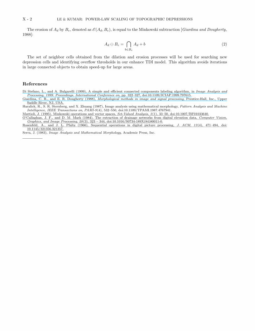
The erosion of Ad by Be, denoted as E (Ad, Be), is equal to the Minkowski subtraction [Giardina and Dougherty ,1988]:

Ad Be =⋂

b∈Be

Ad + b (2)

The set of neighbor cells obtained from the dilation and erosion processes will be used for searching newdepression cells and identifying overflow thresholds in our enhance TDI model. This algorithm avoids iterationsin large connected objects to obtain speed-up for large areas.

References

Di Stefano, L., and A. Bulgarelli (1999), A simple and efficient connected components labeling algorithm, in Image Analysis andProcessing, 1999. Proceedings. International Conference on, pp. 322–327, doi:10.1109/ICIAP.1999.797615.

Giardina, C. R., and E. R. Dougherty (1988), Morphological methods in image and signal processing, Prentice-Hall, Inc., UpperSaddle River, NJ, USA.

Haralick, R., S. R. Sternberg, and X. Zhuang (1987), Image analysis using mathematical morphology, Pattern Analysis and MachineIntelligence, IEEE Transactions on, PAMI-9 (4), 532–550, doi:10.1109/TPAMI.1987.4767941.

Mattioli, J. (1995), Minkowski operations and vector spaces, Set-Valued Analysis, 3 (1), 33–50, doi:10.1007/BF01033640.O’Callaghan, J. F., and D. M. Mark (1984), The extraction of drainage networks from digital elevation data, Computer Vision,

Graphics, and Image Processing, 28 (3), 323 – 344, doi:10.1016/S0734-189X(84)80011-0.Rosenfeld, A., and J. L. Pfaltz (1966), Sequential operations in digital picture processing, J. ACM, 13 (4), 471–494, doi:

10.1145/321356.321357.Serra, J. (1983), Image Analysis and Mathematical Morphology, Academic Press, Inc.

LE & KUMAR: POWER-LAW SCALING OF TOPOGRAPHIC DEPRESSIONS X - 3

(a)

0 10 20

−2

0

2

4

6

8

10

12

14

16

18

20 Original Image(b)

0 10 20

−2

0

2

4

6

8

10

12

14

16

18

20

Dilated Image

Structring Element(c)

0 10 20

−2

0

2

4

6

8

10

12

14

16

18

20

Eroded Image

Structuring Element

Figure S1. Illustration of the dilation and erosion inmathematical morphology to identify neighbor cells oftopographic depressions. (a) Examples of original imagesin different shapes. (b) Dilation of original images usingBd structuring element. (c) Erosion of dilated imagesusing Be structuring element to obtain neighbor cells.

X - 4 LE & KUMAR: POWER-LAW SCALING OF TOPOGRAPHIC DEPRESSIONS

Table

S1.

List

of

para

meters

for

fitted

linea

rreg

ression

lines

an

dgoodness-o

f-fit

test

Site

Lev

elA

reaA

Volu

meV

Dista

nceD

pR

2α

βp

R2

αβ

pR

2α

βµ

[m]

σ[m

]

Christin

aR

iver

Basin

,P

A

l10.4

60.9

3-1

.37

0.7

00.5

40.8

1-0

.84

-0.5

10.7

40.9

9-3

.47

0.9

92.8

91.1

3l2

0.2

00.9

2-1

.37

0.7

60.4

70.8

4-0

.90

-0.4

20.2

30.9

9-3

.35

1.0

03.1

41.5

2l3

0.2

30.9

6-1

.25

0.6

70.0

50.8

0-0

.84

-0.4

40.2

70.9

9-3

.14

1.2

43.1

61.5

5l4

0.0

90.9

0-1

.32

0.7

50.0

20.8

1-0

.86

-0.4

00.2

90.9

8-3

.20

1.3

03.1

71.5

6

Iowa

Riv

erF

loodpla

in,

IA

l10.9

80.9

8-3

.31

1.3

20.9

70.9

6-3

.09

0.7

80.3

20.9

5-2

.85

1.4

02.9

61.3

0l2

0.3

70.9

9-2

.45

0.9

40.2

60.9

7-2

.69

0.6

80.2

00.9

8-3

.18

0.9

23.4

01.6

4l3

0.0

80.9

8-2

.35

0.9

90.2

30.9

8-2

.34

0.5

20.2

50.9

4-2

.87

1.7

33.4

31.6

4l4

0.1

70.9

8-2

.13

0.8

70.4

90.9

5-2

.33

0.5

60.2

90.9

7-3

.03

1.6

43.4

51.6

7

Bird

’sP

oin

tN

ewM

adrid

Flo

odw

ay,M

O

l10.0

80.9

7-1

.54

0.9

50.5

00.9

1-1

.24

-0.7

10.7

70.9

2-2

.63

1.5

42.9

61.2

5l2

0.0

50.9

8-1

.55

1.0

80.2

90.9

7-1

.27

-0.4

10.6

60.9

2-2

.70

1.6

93.3

51.5

2l3

0.6

80.9

9-1

.53

1.1

50.7

60.9

9-1

.30

-0.2

90.2

70.9

4-2

.79

1.5

73.3

81.5

7l4

0.9

40.9

9-1

.51

1.1

50.8

70.9

9-1

.25

-0.2

70.6

80.9

4-2

.85

1.6

23.3

81.5

4

Ow

yhee

Riv

erB

asin

,O

R

l10.8

90.9

5-2

.13

0.9

00.8

20.9

4-1

.53

-0.5

40.7

10.9

9-3

.72

1.2

11.4

81.7

2l2

0.2

10.9

0-2

.07

1.0

60.6

00.8

9-1

.66

-0.2

50.2

20.9

9-3

.69

1.3

21.6

11.9

0l3

0.0

50.8

8-1

.81

0.9

30.1

60.9

2-1

.44

-0.2

60.2

50.9

8-3

.46

1.5

91.6

21.9

3l4

0.1

40.9

0-1

.68

0.8

20.0

50.9

2-1

.47

-0.2

30.3

00.9

8-3

.54

1.6

81.6

21.9

4

Mojav

eD

esert,C

A

l10.0

90.9

3-2

.21

0.3

70.4

50.9

4-2

.13

-0.5

90.7

20.9

8-3

.18

0.7

63.0

41.4

3l2

0.1

00.8

5-1

.85

0.2

20.0

90.9

0-1

.84

-0.6

00.2

00.9

8-3

.15

0.9

63.5

11.8

1l3

0.1

60.8

7-1

.84

0.3

00.1

00.9

0-1

.80

-0.5

50.2

40.9

6-3

.08

1.6

93.5

51.8

5l4

0.1

00.8

9-1

.80

0.3

20.0

10.9

0-1

.81

-0.5

40.3

00.9

5-2

.99

1.6

93.5

61.8

5